Scheduling a Single-Product Reentrant Process with Uniform Processing Times

PROCESS DESIGN AND CONTROL

Scheduling a Single-Product Reentrant Process with UniformProcessing Times

Nitin Lamba, Iftekhar A. Karimi,* and Akesh Bhalla

Department of Chemical and Environmental Engineering, 4 Engineering Drive 4,National University of Singapore, Singapore 117576

Most semiconductor manufacturing involves multiple stages of batch/semicontinuous physico-chemical operations. Scheduling of such plants becomes complex because of a high degree ofreentrancy in their process flows, as different lots/batches as well as different tasks of the samelot compete for time on the various processing units at each stage. Scheduling of a single-productreentrant process with uniform processing times is addressed in this paper. First, an analysisof the minimum possible cycle time in such a process is presented. Then, a one-pass heuristicalgorithm using a novel priority-based resource-sharing policy is developed. The algorithm isalso used to study the impact of the lot release interval on system performance. In comparisonto a previous algorithm, the proposed algorithm is much more efficient and gives much betterresults; thus, it is well suited for a large-scale operation.

Introduction

Increases in the use of computers and high-techgadgetry have boosted the semiconductor manufactur-ing industry tremendously over the past decade. At thesame time, exponential rates of growth and innovationcombined with cutthroat competition are putting tre-mendous pressure on the industry to improve manu-facturing practices and reduce costs. As a result, semi-conductor manufacturing operations have concernedmany researchers in the recent past.

Wafer fabrication is the most important process insemiconductor manufacturing. In a wafer fabricationfacility (or wafer fab), complex electronic circuitry isdeveloped on a polished and clean wafer in a clean room.This is done in multiple passes, each of which creates anew layer (film) with a pattern on the wafer. Thus, awafer has multiple layers embedding several patterns.For instance, a CMOS has 10 layers, whereas a DRAM1

may have 21 or even more layers. Each pass in a waferfabrication process involves some or all of six physico-chemical2 operations (tasks) executed in the followingsequence: (1) Deposit a layer by means of chemicalvapor deposition in a batch furnace. (2) Apply a film oflight-sensitive material, called photoresist, in a spinner-coater assembly. (3) Draw circuitry on a pattern mask,and then use an ultraviolet beam to transfer it to thephotoresist. The photoresist changes its compositionwhere it is exposed to the beam. This entire process(called masking) is carried out in a stepper. (4) Removethe exposed (positive resist) or unexposed (negativeresist) photoresist in a solvent-filled developer bath.(5)Etch the pattern on the wafer layer in a plasma etchchamber using ionized gaseous plasma. Here, theexposed areas of layer are etched away by the plasma.

(6) Strip the entire remaining photoresist layer, if any,in an acid-filled wet-etch bath or an oxygen plasmachamber. Thus, the total number of tasks required tomake a wafer can easily exceed a few hundreds. Allprocessing units in the above six steps are batch units,except for the spinner-coater assembly and stepper.Although these two operate in a semicontinuous mode,the wafers are generally processed in lots; hence, theycan still be treated as batch units. A wafer fab may usemultiple types of units for each step, and there areusually multiple units of each type. For instance, theremay be several types of plasma etch chambers andseveral identical chambers of each type. A set of identi-cal units is called a processing stage (station) or a workcenter. Because the machines involved are usually veryexpensive, economic considerations prohibit allocationof a dedicated station for each pass in a wafer recipe.In other words, a lot may revisit the same stationseveral times during its recipe. This operational featureis called reentrancy, and a wafer fab can be classifiedas a multiproduct network flowshop with identicalparallel units and reentrant flows.

The reentrancy feature creates complex competitionfor resources between similar tasks of different lots,which are at different stages in the recipe, and conflictsinvariably arise. As we shall see later, the manner inwhich these conflicts are resolved can have a majorimpact on the overall process performance. In waferfabs, plant operation is normally regulated (resourceallocation or conflict resolution is achieved) by meansof intelligent lot release and lot scheduling policies. Alot release policy specifies when new lots are introducedinto the plant for production, whereas a lot schedulingpolicy assigns priorities to lots that are competing forthe same processing stage or station. The complexity ofa wafer fab is best illustrated by an example R&D fab3

for which data are shown in Table 1. This fab performs* Corresponding author. E-mail: [email protected].

4203Ind. Eng. Chem. Res. 2000, 39, 4203-4214

10.1021/ie000380x CCC: $19.00 © 2000 American Chemical SocietyPublished on Web 11/06/2000

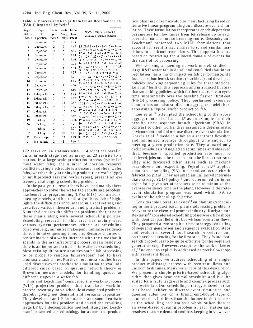
172 tasks on 24 stations with 1-4 identical parallelunits in each stage and as many as 23 revisits to astation. In a large-scale production process (typical ofmost wafer fabs), the number of possible resourceconflicts during a schedule is awesome, and thus, waferfabs, whether they are single-product (one wafer type)or multiproduct (several wafer types), present an ex-tremely challenging scheduling problem.

In the past years, researchers have used mainly threeapproaches to solve the wafer fab scheduling problem:mathematical programming (LP or MIP) formulations,queuing models, and heuristic algorithms. Johri4 high-lights the difficulties encountered in a real setting anddescribes various theoretical and practical problems.Kumar5 discusses the different problems that arise inthese plants along with several scheduling policies.Scheduling research in this area has mainly usedvarious system performance criteria as schedulingobjectives, e.g., minimize makespan, minimize residencetime, minimize queuing time, etc. Because chances ofcontamination of a wafer increase with the time that itspends in the manufacturing process, mean residencetime is an important criterion in wafer fab scheduling.Most existing literature assumes wafer fab processingto be prone to random failure/repair and to havestochastic task times. Furthermore, most studies haveused discrete-event stochastic simulation to evaluatedifferent rules, based on queuing network theory orBrownian network models, for handling queues atdifferent stages in a wafer fab.

Kim and Leachman6 considered the work-in-process(WIP) projection problem that translates work-in-process inventory into a schedule of completed products,thereby giving net demand and resource capacities.They developed an LP formulation and some heuristicapproaches for this problem and solved the resultinglarge LP by a decomposition method. Hung and Leach-man7 presented a methodology for automated produc-

tion planning of semiconductor manufacturing based oniterative linear programming and discrete-event simu-lation. Their formulation incorporates epoch-dependentparameters for flow times from lot release up to eachoperation on each manufacturing route. Dessouky andLeachman8 presented two MILP formulations thataccount for reentrancy, similar lots, and similar ma-chines in semiconductor plants. Their approaches arebased on restricting the allowed domain of events forthe start of lot processing.

Wein,3 using a queuing network model, studied alarge R&D wafer fab in detail and concluded that inputregulation has a major impact on fab performance. Hefocused on bottleneck stations (machines) and developedpolicies involving sequencing rules for these stations.Lu et al.9 built on this approach and introduced fluctua-tion smoothing policies, which further reduce mean cycletime substantially over the baseline first-in-first-out(FIFO) processing policy. They performed extensivesimulations and also studied an aggregate model char-acterizing a typical wafer production fab.

Lee et al.10 attempted the scheduling of the aboveaggregate model of Lu et al.9 as an example for theirnew heuristic sequence branch algorithm (SBA). Incontrast to other works, they assumed a deterministicenvironment and did not use discrete-event simulation.Graves et al.11 modeled a fab as a reentrant flowshopand minimized average throughput time subject tomeeting a given production rate. They allowed onlycyclic schedules and neglected setup times and observedthat, because a specified production rate must beachieved, jobs must be released into the line at that rate.They also discussed other issues such as machinebreakdowns and expediting. Peyrol et al.12 appliedsimulated annealing (SA) to a semiconductor circuitfabrication plant. They assumed an unlimited interme-diate storage (UIS) policy13 and determined an inputorder for a given set of products so as to minimize theaverage residence time in the plant. However, a discrete-event simulation program was used within SA toevaluate the scheduling objective.

Considerable literature exists14 on planning/schedul-ing in multiproduct batch plants addressing problemsrelevant to the chemical process industry. Kuriyan andReklaitis15 considered scheduling of network flowshopswith identical parallel units but without reentrant flows.They proposed a two-step heuristic strategy consistingof sequence generation and sequence evaluation stepsand evaluated several local search procedures andbottleneck sequencing for the first step. They found localsearch procedures to be quite effective for the sequencegeneration step. However, except for the work of Lee etal.,10 no one has explicitly addressed network flowshopswith reentrant flows.

In this paper, we address scheduling of a single-product multistage process with reentrant flows anduniform task times. Many wafer fabs fit this description.We present a simple priority-based scheduling algo-rithm that gives near optimal schedules and is quitesuited for a truly large-scale and complex process suchas a wafer fab. Our scheduling strategy is novel in thatit is based neither on discrete-event simulation andqueuing rules nor on a branch-and-bound type ofenumeration. It differs from the former in that it looksat the scheduling problem as a whole rather than asan event-based queuing problem at each station andresolves resource demand conflicts keeping in view even

Table 1. Process and Recipe Data for an R&D Wafer Fab(FAB 1) Reported by Wein3

4204 Ind. Eng. Chem. Res., Vol. 39, No. 11, 2000

future demands and not just the present ones. We alsodevelop a recipe representation that suits our algorithmand provides a framework for uniform treatment ofresources (machines, utilities, operators, etc.) in thistype of reentrant flowshop. Although developed with adeterministic process in mind, the algorithm is also usedto study a stochastic process with little modification.

In the following section, we first state the problemaddressed in this paper and then present an analysisof minimum cycle time in order to derive two lowerbounds on the makespan. Subsequently, we describe ouralgorithm and illustrate its application by means of twoexamples. Finally, we also study the effect of the lotrelease interval and stochastic processing times for oneof the examples.

Problem Statement

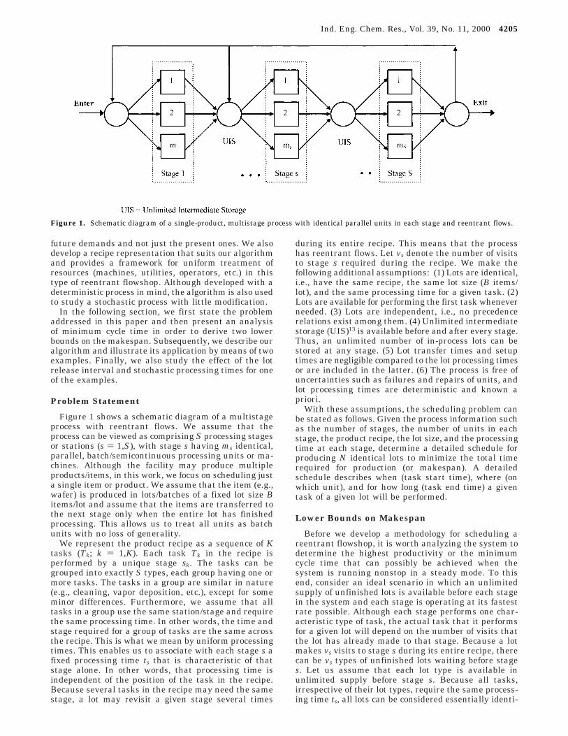
Figure 1 shows a schematic diagram of a multistageprocess with reentrant flows. We assume that theprocess can be viewed as comprising S processing stagesor stations (s ) 1,S), with stage s having ms identical,parallel, batch/semicontinuous processing units or ma-chines. Although the facility may produce multipleproducts/items, in this work, we focus on scheduling justa single item or product. We assume that the item (e.g.,wafer) is produced in lots/batches of a fixed lot size Bitems/lot and assume that the items are transferred tothe next stage only when the entire lot has finishedprocessing. This allows us to treat all units as batchunits with no loss of generality.

We represent the product recipe as a sequence of Ktasks (Tk; k ) 1,K). Each task Tk in the recipe isperformed by a unique stage sk. The tasks can begrouped into exactly S types, each group having one ormore tasks. The tasks in a group are similar in nature(e.g., cleaning, vapor deposition, etc.), except for someminor differences. Furthermore, we assume that alltasks in a group use the same station/stage and requirethe same processing time. In other words, the time andstage required for a group of tasks are the same acrossthe recipe. This is what we mean by uniform processingtimes. This enables us to associate with each stage s afixed processing time ts that is characteristic of thatstage alone. In other words, that processing time isindependent of the position of the task in the recipe.Because several tasks in the recipe may need the samestage, a lot may revisit a given stage several times

during its entire recipe. This means that the processhas reentrant flows. Let vs denote the number of visitsto stage s required during the recipe. We make thefollowing additional assumptions: (1) Lots are identical,i.e., have the same recipe, the same lot size (B items/lot), and the same processing time for a given task. (2)Lots are available for performing the first task wheneverneeded. (3) Lots are independent, i.e., no precedencerelations exist among them. (4) Unlimited intermediatestorage (UIS)13 is available before and after every stage.Thus, an unlimited number of in-process lots can bestored at any stage. (5) Lot transfer times and setuptimes are negligible compared to the lot processing timesor are included in the latter. (6) The process is free ofuncertainties such as failures and repairs of units, andlot processing times are deterministic and known apriori.

With these assumptions, the scheduling problem canbe stated as follows. Given the process information suchas the number of stages, the number of units in eachstage, the product recipe, the lot size, and the processingtime at each stage, determine a detailed schedule forproducing N identical lots to minimize the total timerequired for production (or makespan). A detailedschedule describes when (task start time), where (onwhich unit), and for how long (task end time) a giventask of a given lot will be performed.

Lower Bounds on Makespan

Before we develop a methodology for scheduling areentrant flowshop, it is worth analyzing the system todetermine the highest productivity or the minimumcycle time that can possibly be achieved when thesystem is running nonstop in a steady mode. To thisend, consider an ideal scenario in which an unlimitedsupply of unfinished lots is available before each stagein the system and each stage is operating at its fastestrate possible. Although each stage performs one char-acteristic type of task, the actual task that it performsfor a given lot will depend on the number of visits thatthe lot has already made to that stage. Because a lotmakes vs visits to stage s during its entire recipe, therecan be vs types of unfinished lots waiting before stages. Let us assume that each lot type is available inunlimited supply before stage s. Because all tasks,irrespective of their lot types, require the same process-ing time ts, all lots can be considered essentially identi-

Figure 1. Schematic diagram of a single-product, multistage process with identical parallel units in each stage and reentrant flows.

Ind. Eng. Chem. Res., Vol. 39, No. 11, 2000 4205

cal as far as the operation of stage s is concerned. Inthis ideal scenario, it is clear that the minimum timebetween the emergence of two successive lots from stages is ts/ms. Because the total processing time of a lot onstage s is vsts, the minimum average time between theemergence of two successive lots of the same type fromstage s, or the minimum average cycle time of stage s,is given by

We define the above as the minimum stage cycle time.Its inverse gives the fastest processing rate (lots per unittime) that stage s can achieve under the ideal scenariodefined earlier. As expected, for the special case of vs )1 and ms ) 1, eq 1 reduces to the lot processing time onstage s. Because a lot has to pass through S stages inseries with different processing rates, the slowest stagewill be the bottleneck or the rate-limiting stage. Thus,the minimum average cycle time for the S-stage serialprocess, or equivalently the minimum average processcycle time, is given by

Note that the term cycle time, as used in the semicon-ductor manufacturing parlance,9 refers to the residencetime and not the cycle time as used here. Residencetime, by itself, is also an important performance crite-rion, as it impacts yield losses.9

From the above analysis, it is clear that finished lotscannot be produced at an average rate greater than 1/t*when the fab is operating with unlimited intermediatestorage levels as described above. To produce N lots, letus assume that each stage begins operation at time zero,operates at its fastest rate, and stops operation when ithas processed all of the tasks that it needs to performto produce exactly N lots. It is clear that the rate-limiting stage will finish last and at time Nt*.

In a real situation (where unlimited supplies are notavailable), however, the stages will have to wait for theirpredecessors to finish tasks, and thus the time required

will be no less than Nt*. The situation becomes morecomplex when we start with an empty system. It is clearthat the makespan cannot be lower than v1t1 + v2t2 +v3t3 + ... + vStS, the minimum residence time for thefirst lot. On the basis of this discussion, it is verytempting to propose a lower bound LB1 on the makespanas

In most cases, this is a very good lower bound. However,this can, indeed, be violated by the first few lots.Because the fab is empty initially, there are several timeslots on the machines, which can facilitate schedulingin such a way that the limiting stage/step is not the rate-controlling step. Let us illustrate this with an example.

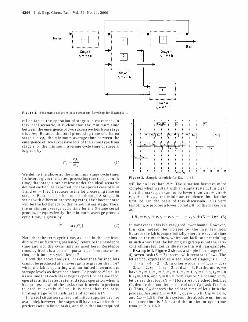
Example I. Figure 2 shows a simple four-stage (S )4), seven-task (K ) 7) process with reentrant flows. Thelot recipe, expressed as a sequence of stages, is 1 f 2f 3 f 2 f 4 f 2 f 3. In other words, s1 ) 1, s2 ) 2, s3) 3, s4 ) 2, s5 ) 4, s6 ) 2, and s7 ) 3. Furthermore, wehave m1 ) 1, m2 ) 2, m3 ) 1, m4 ) 1, t1 ) 0.5 h, t2 ) 1.0h, t3 ) 0.8 h, and t4 ) 0.5 h from Figure 2. For simplicity,let us say that four (N ) 4) lots are to be scheduled. LetCik denote the completion time of task Tik (task Tk of loti). Thus, Ci0 denotes the release time of lot i into theprocess. Assume C10 ) 0.0 h, C20 ) 0.5 h, C30 ) 1.0 h,and C40 ) 1.5 h. For this system, the absolute minimumresidence time is 5.6 h, and the minimum cycle timefrom eq 2 is 1.6 h.

Figure 2. Schematic diagram of a reentrant flowshop for Example I.

t*s )vsts

ms(1)

t* ) maxs

[t*s] (2)

Figure 3. Sample schedule for Example I.

LB1 ) v1t1 + v2t2 + v3t3 + ... + vStS + (N - 1)t* (3)


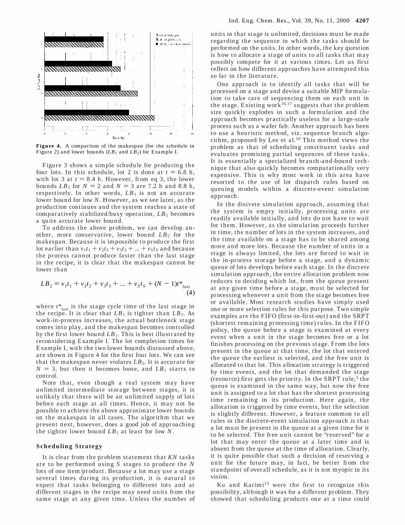
Figure 3 shows a simple schedule for producing thefour lots. In this schedule, lot 2 is done at t ) 6.8 h,with lot 3 at t ) 8.4 h. However, from eq 3, the lowerbounds LB1 for N ) 2 and N ) 3 are 7.2 h and 8.8 h,respectively. In other words, LB1 is not an accuratelower bound for low N. However, as we see later, as theproduction continues and the system reaches a state ofcomparatively stabilized/busy operation, LB1 becomesa quite accurate lower bound.

To address the above problem, we can develop an-other, more conservative, lower bound LB2 for themakespan. Because it is impossible to produce the firstlot earlier than v1t1 + v2t2 + v3t3 + ... + vStS and becausethe process cannot produce faster than the last stagein the recipe, it is clear that the makespan cannot belower than

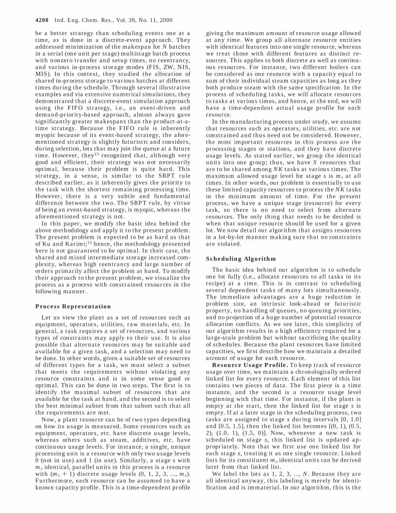
where t*last is the stage cycle time of the last stage inthe recipe. It is clear that LB1 is tighter than LB2. Aswork-in-process increases, the actual bottleneck stagecomes into play, and the makespan becomes controlledby the first lower bound LB1. This is best illustrated byreconsidering Example I. The lot completion times forExample I, with the two lower bounds discussed above,are shown in Figure 4 for the first four lots. We can seethat the makespan never violates LB2. It is accurate forN ) 3, but then it becomes loose, and LB1 starts tocontrol.

Note that, even though a real system may haveunlimited intermediate storage between stages, it isunlikely that there will be an unlimited supply of lotsbefore each stage at all times. Hence, it may not bepossible to achieve the above approximate lower boundson the makespan in all cases. The algorithm that wepresent next, however, does a good job of approachingthe tighter lower bound LB1 at least for low N.

Scheduling Strategy

It is clear from the problem statement that KN tasksare to be performed using S stages to produce the Nlots of one item/product. Because a lot may use a stageseveral times during its production, it is natural toexpect that tasks belonging to different lots and atdifferent stages in the recipe may need units from thesame stage at any given time. Unless the number of

units in that stage is unlimited, decisions must be maderegarding the sequence in which the tasks should beperformed on the units. In other words, the key questionis how to allocate a stage of units to all tasks that maypossibly compete for it at various times. Let us firstreflect on how different approaches have attempted thisso far in the literature.

One approach is to identify all tasks that will beprocessed on a stage and devise a suitable MIP formula-tion to take care of sequencing them on each unit inthe stage. Existing work16,17 suggests that the problemsize quickly explodes in such a formulation and theapproach becomes practically useless for a large-scaleprocess such as a wafer fab. Another approach has beento use a heuristic method, viz. sequence branch algo-rithm, proposed by Lee et al.10 This method views theproblem as that of scheduling constituent tasks andevaluates promising partial sequences of these tasks.It is essentially a specialized branch-and-bound tech-nique that also quickly becomes computationally veryexpensive. This is why most work in this area haveresorted to the use of lot dispatch rules based onqueuing models within a discrete-event simulationapproach.

In the discrete simulation approach, assuming thatthe system is empty initially, processing units arereadily available initially, and lots do not have to waitfor them. However, as the simulation proceeds furtherin time, the number of lots in the system increases, andthe time available on a stage has to be shared amongmore and more lots. Because the number of units in astage is always limited, the lots are forced to wait inthe in-process storage before a stage, and a dynamicqueue of lots develops before each stage. In the discretesimulation approach, the entire allocation problem nowreduces to deciding which lot, from the queue presentat any given time before a stage, must be selected forprocessing whenever a unit from the stage becomes freeor available. Most research studies have simply usedone or more selection rules for this purpose. Two simpleexamples are the FIFO (first-in-first-out) and the SRPT(shortest remaining processing time) rules. In the FIFOpolicy, the queue before a stage is examined at everyevent when a unit in the stage becomes free or a lotfinishes processing on the previous stage. From the lotspresent in the queue at that time, the lot that enteredthe queue the earliest is selected, and the free unit isallocated to that lot. This allocation strategy is triggeredby time events, and the lot that demanded the stage(resource) first gets the priority. In the SRPT rule,3 thequeue is examined in the same way, but now the freeunit is assigned to a lot that has the shortest processingtime remaining in its production. Here again, theallocation is triggered by time events, but the selectionis slightly different. However, a feature common to allrules in the discrete-event simulation approach is thata lot must be present in the queue at a given time for itto be selected. The free unit cannot be “reserved” for alot that may enter the queue at a later time and isabsent from the queue at the time of allocation. Clearly,it is quite possible that such a decision of reserving aunit for the future may, in fact, be better from thestandpoint of overall schedule, as it is not myopic in itsvision.

Ku and Karimi13 were the first to recognize thispossibility, although it was for a different problem. Theyshowed that scheduling products one at a time could

Figure 4. A comparison of the makespan (for the schedule inFigure 2) and lower bounds (LB1 and LB2) for Example I.

LB2 ) v1t1 + v2t2 + v3t3 + ... + vStS + (N - 1)t*last(4)


be a better strategy than scheduling events one at atime, as is done in a discrete-event approach. Theyaddressed minimization of the makespan for N batchesin a serial (one unit per stage) multistage batch processwith nonzero transfer and setup times, no reentrancy,and various in-process storage modes (FIS, ZW, NIS,MIS). In this context, they studied the allocation ofshared in-process storage to various batches at differenttimes during the schedule. Through several illustrativeexamples and via extensive numerical simulations, theydemonstrated that a discrete-event simulation approachusing the FIFO strategy, i.e., an event-driven anddemand-priority-based approach, almost always gavesignificantly greater makespans than the product-at-a-time strategy. Because the FIFO rule is inherentlymyopic because of its event-based strategy, the afore-mentioned strategy is slightly futuristic and considers,during selection, lots that may join the queue at a futuretime. However, they13 recognized that, although verygood and efficient, their strategy was not necessarilyoptimal, because their problem is quite hard. Thisstrategy, in a sense, is similar to the SRPT ruledescribed earlier, as it inherently gives the priority tothe task with the shortest remaining processing time.However, there is a very subtle and fundamentaldifference between the two. The SRPT rule, by virtueof being an event-based strategy, is myopic, whereas theaforementioned strategy is not.

In this paper, we modify the basic idea behind theabove methodology and apply it to the present problem.The present problem is expected to be as hard as thatof Ku and Karimi;13 hence, the methodology presentedhere is not guaranteed to be optimal. In their case, theshared and mixed intermediate storage increased com-plexity, whereas high reentrancy and large number oforders primarily affect the problem at hand. To modifytheir approach to the present problem, we visualize theprocess as a process with constrained resources in thefollowing manner.

Process Representation

Let us view the plant as a set of resources such asequipment, operators, utilities, raw materials, etc. Ingeneral, a task requires a set of resources, and varioustypes of constraints may apply to their use. It is alsopossible that alternate resources may be suitable andavailable for a given task, and a selection may need tobe done. In other words, given a suitable set of resourcesof different types for a task, we must select a subsetthat meets the requirements without violating anyresource constraints and is in some sense good oroptimal. This can be done in two steps. The first is toidentify the maximal subset of resources that areavailable for the task at hand, and the second is to selectthe best minimal subset from that subset such that allthe requirements are met.

Now, a plant resource can be of two types dependingon how its usage is measured. Some resources such asequipment, operators, etc. have discrete usage levels,whereas others such as steam, additives, etc. havecontinuous usage levels. For instance, a single, uniqueprocessing unit is a resource with only two usage levels0 (not in use) and 1 (in use). Similarly, a stage s withms identical, parallel units in this process is a resourcewith (ms + 1) discrete usage levels (0, 1, 2, 3, ..., ms).Furthermore, each resource can be assumed to have aknown capacity profile. This is a time-dependent profile

giving the maximum amount of resource usage allowedat any time. We group all alternate resource entitieswith identical features into one single resource, whereaswe treat those with different features as distinct re-sources. This applies to both discrete as well as continu-ous resources. For instance, two different boilers canbe considered as one resource with a capacity equal tosum of their individual steam capacities as long as theyboth produce steam with the same specification. In theprocess of scheduling tasks, we will allocate resourcesto tasks at various times, and hence, at the end, we willhave a time-dependent actual usage profile for eachresource.

In the manufacturing process under study, we assumethat resources such as operators, utilities, etc. are notconstrained and thus need not be considered. However,the most important resources in this process are theprocessing stages or stations, and they have discreteusage levels. As stated earlier, we group the identicalunits into one group; thus, we have S resources thatare to be shared among NK tasks at various times. Themaximum allowed usage level for stage s is ms at alltimes. In other words, our problem is essentially to usethese limited capacity resources to process the NK tasksin the minimum amount of time. For the presentprocess, we have a unique stage (resource) for everytask, so there is no need to select from alternateresources. The only thing that needs to be decided iswhen that unique resource should be used for a givenlot. We now detail our algorithm that assigns resourcesin a lot-by-lot manner making sure that no constraintsare violated.

Scheduling Algorithm

The basic idea behind our algorithm is to scheduleone lot fully (i.e., allocate resources to all tasks in itsrecipe) at a time. This is in contrast to schedulingseveral dependent tasks of many lots simultaneously.The immediate advantages are a huge reduction inproblem size, an intrinsic look-ahead or futuristicproperty, no handling of queues, no queuing priorities,and no projection of a huge number of potential resourceallocation conflicts. As we see later, this simplicity ofour algorithm results in a high efficiency required for alarge-scale problem but without sacrificing the qualityof schedules. Because the plant resources have limitedcapacities, we first describe how we maintain a detailedaccount of usage for each resource.

Resource Usage Profile. To keep track of resourceusage over time, we maintain a chronologically orderedlinked list for every resource. Each element of this listcontains two pieces of data. The first piece is a timeinstance, and the second is a resource usage levelbeginning with that time. For instance, if the plant isempty at the start, then the linked list for stage s isempty. If at a later stage in the scheduling process, twotasks are assigned to stage s during intervals [0, 1.0]and [0.5, 1.5], then the linked list becomes [(0, 1), (0.5,2), (1.0, 1), (1.5, 0)]. Now, whenever a new task isscheduled on stage s, this linked list is updated ap-propriately. Note that we first use one linked list foreach stage s, treating it as one single resource. Linkedlists for its constituent ms identical units can be derivedlater from that linked list.

We label the lots as 1, 2, 3, ..., N. Because they areall identical anyway, this labeling is merely for identi-fication and is immaterial. In our algorithm, this is the


order in which lots enter the process, i.e., are releasedinto the process, and also the order in which they arescheduled one at a time. For each lot, tasks are alsoscheduled one at a time in the sequence T1, T2, T3, ...,TK. With this, our algorithm can be simply stated asfollows:Step 1: Initialize plant state at time zero.Schedule: Do i ) 1, N

Do k ) 1, KStep 2: Schedule task Tik (defined as task Tk of

lot i)End Do: ScheduleStep 3: Assign a specific processing unit to each taskWe now describe the above three steps in detail.

Step 1: Initialize Plant State. Here, we create onelinked list or usage profile for each stage. If the plantis empty at the start, then all linked lists are empty. Ifthis is not so, then we assume that a schedule for theunfinished lots is available, with which the link listscan be initialized. If this is not so either, then we firstschedule all of the unfinished lots using our algorithmstated above to obtain the initial plant state.

Step 2: Schedule Task Tik. As mentioned earlier, thelot release policy is an important scheduling decision.Several release policies3 have been proposed. The sim-plest is a deterministic one, in which lots are releasedinto the system at a fixed, predetermined time interval.For now, we assume that lot release times Ci0 are knowna priori and consider how to schedule task Tik.

Because lot transfer times and setup times arenegligible, it is clear that Ci(k-1), the completion time ofTi(k-1), is the earliest time at which task Tik can begin.To perform Tik, we need one free unit from stage sk forduration pk, where pk denotes the time required toperform Tik. For this, we search the linked list for stagesk, beginning with time Ci(k-1), to locate the earliest timeslot of length pk during which the usage level of sk isless than its capacity. We allocate stage sk to Tik for thatslot and update the linked list of sk to reflect thisallocation. Thus, the resource usage profiles are con-tinually updated after each scheduled task, and anyallocation, once done, cannot be revised again later. Werecord the start time of this slot as the start time of Tikand the end time of this slot as the end time (Cik) of Tik.

From the above discussion, it is clear that ouralgorithm gives higher priority to lots earlier in thesequence than to those later in the sequence, as far asresource allocation is concerned. A resource, once as-signed to a task for a given duration, cannot be reas-signed to another task for that duration. Thus, everytask is scheduled subject to the schedule and resourceallocations of all previous tasks. Furthermore, thealgorithm schedules every task so as to complete it asearly as possible subject to the available resources plusthe completion time of its precursor task in the recipe.Finally, by its very nature, it never makes any allocationthat would violate resource constraints.

Step 3: Assign units to tasks. From the scheduleobtained so far, we know when a task will startprocessing on a particular stage and when it will end,but we do not know exactly which unit it will use inthat stage. We now present an algorithm to assign adistinct unit to each task using the final linked lists forthe entire schedule. In step 2, we treated each stage asa single resource with a certain capacity and made surethat its usage never exceeded its capacity. This meansthat at least one unit in a stage is surely free at every

instance between the start and end times of every taskto be processed on that stage. However, how do we knowif we can process that task on one and the same unitfor the entire duration? Is it possible that one unit isfree for a part of the time, after which it is not free, butanother unit becomes free, and so the task must beswitched to that unit? We call this task splitting. Thus,is it possible that task splitting may arise, when we tryto assign units to tasks based on the cumulative usageprofile for a stage? This says that the assignment ofunits to tasks may not be a trivial problem. For a givenstage usage profile, many different assignments of unitsto tasks are possible, and an optimal solution may exist.Fortunately, in this study, because each stage consistsof identical units, the process of obtaining one feasibleassignment of units to tasks without task splitting isstraightforward.

The key to avoid task splitting is not to think ofassigning units to tasks based on priority as is done inthe scheduling algorithm, but to assign them based ona FIFO policy. To this end, we process all tasks on astage, one at a time, in increasing order of their starttimes and assign a free unit to each task while account-ing the usage of each individual unit in that stage. Fora stage s, we proceed as follows: (1) Take the finallinked list for stage s and process its elements one byone. Recall that the elements in the linked list areordered chronologically and each element denotes a timeinstance and one or more events (i.e., the start and/orend of one or more tasks) that happen at that time.While processing the linked list, we maintain an endtime for each unit in stage s. This is the time at whichthe unit becomes free after finishing the last taskassigned to it. At the start, these end times are obtainedfrom the initial state of the plant. (2) Now let us saythat we have already processed the first (n - 1)elements of the linked list and we wish to process thenth element. Let this element denote a time instance tin the schedule. If no task starts at time t, then nothingneeds to be done, and we proceed to the next element.For each task that starts at time t, we assign a unit forit as follows. (3) We compare the current end times ofall units with the current time t. If the end time of aunit exceeds t, then that unit is not available. If the endtime of a unit is earlier than t, then that unit is availablefor this task. Because multiple units may be available,we need a selection criterion to choose one from amongthem. In this study, we select the available unit whosecurrent end time is the nearest to t and assign it to thetask. Knowing the task time, we now update the endtime for this unit. (4) Processing of the nth element iscomplete when all tasks that start at t are assignedunits. We then proceed to the next element and repeatsteps 2 and 3. When all elements in the linked list areprocessed, all tasks will have been assigned units.

The above procedure is guaranteed to give assign-ments without violating the stage capacity and withoutany task splitting, because every stage usage profileensures that a free unit will always be available at thestart of every task on that stage and the stage capacitywill not be violated at any time during the entireschedule.

Remarks. In this problem, there is a unique suitableresource for every task, and hence, the question ofselecting from alternate resources did not arise. In ageneral problem, there can be several alternate re-sources for every task, and then one must use some


selection criteria to pick one from the alternate availableresources. This will normally involve examining thelinked lists of all the alternate resources to determinetheir availabilities plus some other criteria for selectingthe best. One simple criterion could be that the earliestavailable resource should be selected first. In any case,the point is that we can easily extend this algorithm toaccommodate multiple alternate resources.

Next, we illustrate our algorithm via two examples.The first example (Example I, Figure 2, discussedearlier) illustrates the algorithmic steps in detail,whereas the second, more complex, example demon-strates and evaluates the full potential and effectivenessof our algorithm.

Example I (Revisited)

We first create four linked lists L1, L2, L3, and L4respectively for stages 1-4. Assuming the plant to beempty at the start, all lists are initially empty. Thiscompletes the plant initialization step of our algorithm.

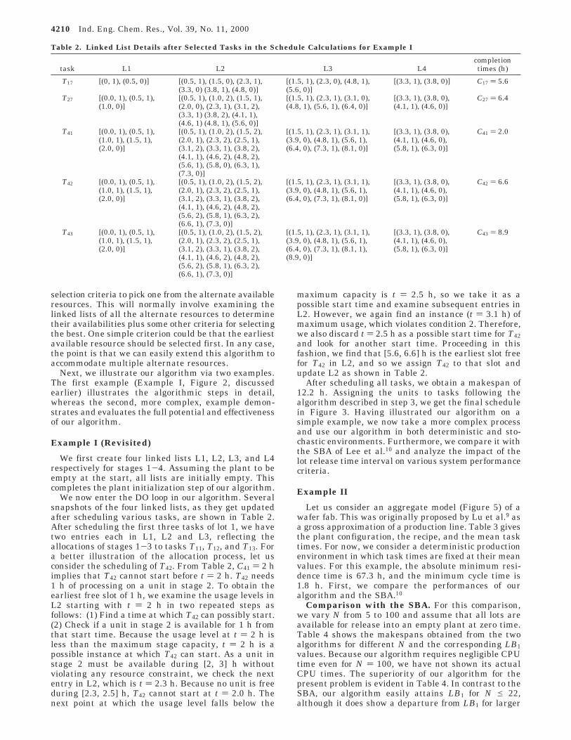
We now enter the DO loop in our algorithm. Severalsnapshots of the four linked lists, as they get updatedafter scheduling various tasks, are shown in Table 2.After scheduling the first three tasks of lot 1, we havetwo entries each in L1, L2 and L3, reflecting theallocations of stages 1-3 to tasks T11, T12, and T13. Fora better illustration of the allocation process, let usconsider the scheduling of T42. From Table 2, C41 ) 2 himplies that T42 cannot start before t ) 2 h. T42 needs1 h of processing on a unit in stage 2. To obtain theearliest free slot of 1 h, we examine the usage levels inL2 starting with t ) 2 h in two repeated steps asfollows: (1) Find a time at which T42 can possibly start.(2) Check if a unit in stage 2 is available for 1 h fromthat start time. Because the usage level at t ) 2 h isless than the maximum stage capacity, t ) 2 h is apossible instance at which T42 can start. As a unit instage 2 must be available during [2, 3] h withoutviolating any resource constraint, we check the nextentry in L2, which is t ) 2.3 h. Because no unit is freeduring [2.3, 2.5] h, T42 cannot start at t ) 2.0 h. Thenext point at which the usage level falls below the

maximum capacity is t ) 2.5 h, so we take it as apossible start time and examine subsequent entries inL2. However, we again find an instance (t ) 3.1 h) ofmaximum usage, which violates condition 2. Therefore,we also discard t ) 2.5 h as a possible start time for T42and look for another start time. Proceeding in thisfashion, we find that [5.6, 6.6] h is the earliest slot freefor T42 in L2, and so we assign T42 to that slot andupdate L2 as shown in Table 2.

After scheduling all tasks, we obtain a makespan of12.2 h. Assigning the units to tasks following thealgorithm described in step 3, we get the final schedulein Figure 3. Having illustrated our algorithm on asimple example, we now take a more complex processand use our algorithm in both deterministic and sto-chastic environments. Furthermore, we compare it withthe SBA of Lee et al.10 and analyze the impact of thelot release time interval on various system performancecriteria.

Example II

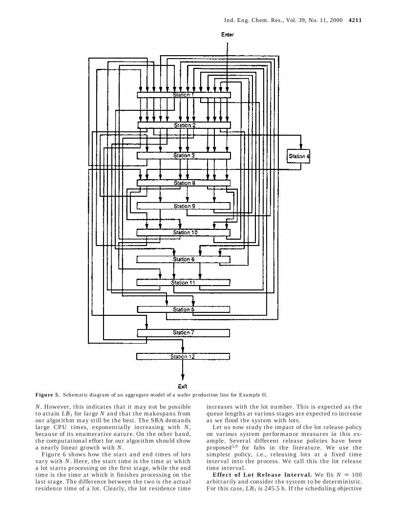
Let us consider an aggregate model (Figure 5) of awafer fab. This was originally proposed by Lu et al.9 asa gross approximation of a production line. Table 3 givesthe plant configuration, the recipe, and the mean tasktimes. For now, we consider a deterministic productionenvironment in which task times are fixed at their meanvalues. For this example, the absolute minimum resi-dence time is 67.3 h, and the minimum cycle time is1.8 h. First, we compare the performances of ouralgorithm and the SBA.10

Comparison with the SBA. For this comparison,we vary N from 5 to 100 and assume that all lots areavailable for release into an empty plant at zero time.Table 4 shows the makespans obtained from the twoalgorithms for different N and the corresponding LB1values. Because our algorithm requires negligible CPUtime even for N ) 100, we have not shown its actualCPU times. The superiority of our algorithm for thepresent problem is evident in Table 4. In contrast to theSBA, our algorithm easily attains LB1 for N e 22,although it does show a departure from LB1 for larger

Table 2. Linked List Details after Selected Tasks in the Schedule Calculations for Example I

task L1 L2 L3 L4completiontimes (h)

T17 [(0, 1), (0.5, 0)] [(0.5, 1), (1.5, 0), (2.3, 1),(3.3, 0) (3.8, 1), (4.8, 0)]

[(1.5, 1), (2.3, 0), (4.8, 1),(5.6, 0)]

[(3.3, 1), (3.8, 0)] C17 ) 5.6

T27 [(0.0, 1), (0.5, 1),(1.0, 0)]

[(0.5, 1), (1.0, 2), (1.5, 1),(2.0, 0), (2.3, 1), (3.1, 2),(3.3, 1) (3.8, 2), (4.1, 1),(4.6, 1) (4.8, 1), (5.6, 0)]

[(1.5, 1), (2.3, 1), (3.1, 0),(4.8, 1), (5.6, 1), (6.4, 0)]

[(3.3, 1), (3.8, 0),(4.1, 1), (4.6, 0)]

C27 ) 6.4

T41 [(0.0, 1), (0.5, 1),(1.0, 1), (1.5, 1),(2.0, 0)]

[(0.5, 1), (1.0, 2), (1.5, 2),(2.0, 1), (2.3, 2), (2.5, 1),(3.1, 2), (3.3, 1), (3.8, 2),(4.1, 1), (4.6, 2), (4.8, 2),(5.6, 1), (5.8, 0), (6.3, 1),(7.3, 0)]

[(1.5, 1), (2.3, 1), (3.1, 1),(3.9, 0), (4.8, 1), (5.6, 1),(6.4, 0), (7.3, 1), (8.1, 0)]

[(3.3, 1), (3.8, 0),(4.1, 1), (4.6, 0),(5.8, 1), (6.3, 0)]

C41 ) 2.0

T42 [(0.0, 1), (0.5, 1),(1.0, 1), (1.5, 1),(2.0, 0)]

[(0.5, 1), (1.0, 2), (1.5, 2),(2.0, 1), (2.3, 2), (2.5, 1),(3.1, 2), (3.3, 1), (3.8, 2),(4.1, 1), (4.6, 2), (4.8, 2),(5.6, 2), (5.8, 1), (6.3, 2),(6.6, 1), (7.3, 0)]

[(1.5, 1), (2.3, 1), (3.1, 1),(3.9, 0), (4.8, 1), (5.6, 1),(6.4, 0), (7.3, 1), (8.1, 0)]

[(3.3, 1), (3.8, 0),(4.1, 1), (4.6, 0),(5.8, 1), (6.3, 0)]

C42 ) 6.6

T43 [(0.0, 1), (0.5, 1),(1.0, 1), (1.5, 1),(2.0, 0)]

[(0.5, 1), (1.0, 2), (1.5, 2),(2.0, 1), (2.3, 2), (2.5, 1),(3.1, 2), (3.3, 1), (3.8, 2),(4.1, 1), (4.6, 2), (4.8, 2),(5.6, 2), (5.8, 1), (6.3, 2),(6.6, 1), (7.3, 0)]

[(1.5, 1), (2.3, 1), (3.1, 1),(3.9, 0), (4.8, 1), (5.6, 1),(6.4, 0), (7.3, 1), (8.1, 1),(8.9, 0)]

[(3.3, 1), (3.8, 0),(4.1, 1), (4.6, 0),(5.8, 1), (6.3, 0)]

C43 ) 8.9


N. However, this indicates that it may not be possibleto attain LB1 for large N and that the makespans fromour algorithm may still be the best. The SBA demandslarge CPU times, exponentially increasing with N,because of its enumerative nature. On the other hand,the computational effort for our algorithm should showa nearly linear growth with N.

Figure 6 shows how the start and end times of lotsvary with N. Here, the start time is the time at whicha lot starts processing on the first stage, while the endtime is the time at which it finishes processing on thelast stage. The difference between the two is the actualresidence time of a lot. Clearly, the lot residence time

increases with the lot number. This is expected as thequeue lengths at various stages are expected to increaseas we flood the system with lots.

Let us now study the impact of the lot release policyon various system performance measures in this ex-ample. Several different release policies have beenproposed3,9 for fabs in the literature. We use thesimplest policy, i.e., releasing lots at a fixed timeinterval into the process. We call this the lot releasetime interval.

Effect of Lot Release Interval. We fix N ) 100arbitrarily and consider the system to be deterministic.For this case, LB1 is 245.5 h. If the scheduling objective

Figure 5. Schematic diagram of an aggregate model of a wafer production line for Example II.


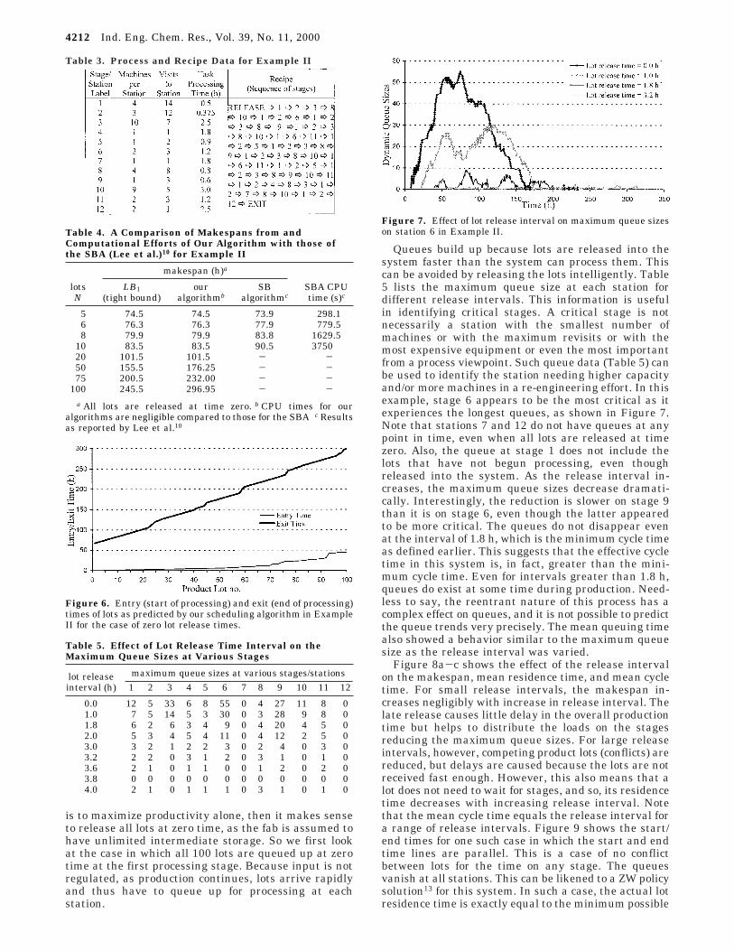
is to maximize productivity alone, then it makes senseto release all lots at zero time, as the fab is assumed tohave unlimited intermediate storage. So we first lookat the case in which all 100 lots are queued up at zerotime at the first processing stage. Because input is notregulated, as production continues, lots arrive rapidlyand thus have to queue up for processing at eachstation.

Queues build up because lots are released into thesystem faster than the system can process them. Thiscan be avoided by releasing the lots intelligently. Table5 lists the maximum queue size at each station fordifferent release intervals. This information is usefulin identifying critical stages. A critical stage is notnecessarily a station with the smallest number ofmachines or with the maximum revisits or with themost expensive equipment or even the most importantfrom a process viewpoint. Such queue data (Table 5) canbe used to identify the station needing higher capacityand/or more machines in a re-engineering effort. In thisexample, stage 6 appears to be the most critical as itexperiences the longest queues, as shown in Figure 7.Note that stations 7 and 12 do not have queues at anypoint in time, even when all lots are released at timezero. Also, the queue at stage 1 does not include thelots that have not begun processing, even thoughreleased into the system. As the release interval in-creases, the maximum queue sizes decrease dramati-cally. Interestingly, the reduction is slower on stage 9than it is on stage 6, even though the latter appearedto be more critical. The queues do not disappear evenat the interval of 1.8 h, which is the minimum cycle timeas defined earlier. This suggests that the effective cycletime in this system is, in fact, greater than the mini-mum cycle time. Even for intervals greater than 1.8 h,queues do exist at some time during production. Need-less to say, the reentrant nature of this process has acomplex effect on queues, and it is not possible to predictthe queue trends very precisely. The mean queuing timealso showed a behavior similar to the maximum queuesize as the release interval was varied.

Figure 8a-c shows the effect of the release intervalon the makespan, mean residence time, and mean cycletime. For small release intervals, the makespan in-creases negligibly with increase in release interval. Thelate release causes little delay in the overall productiontime but helps to distribute the loads on the stagesreducing the maximum queue sizes. For large releaseintervals, however, competing product lots (conflicts) arereduced, but delays are caused because the lots are notreceived fast enough. However, this also means that alot does not need to wait for stages, and so, its residencetime decreases with increasing release interval. Notethat the mean cycle time equals the release interval fora range of release intervals. Figure 9 shows the start/end times for one such case in which the start and endtime lines are parallel. This is a case of no conflictbetween lots for the time on any stage. The queuesvanish at all stations. This can be likened to a ZW policysolution13 for this system. In such a case, the actual lotresidence time is exactly equal to the minimum possible

Table 3. Process and Recipe Data for Example II

Table 4. A Comparison of Makespans from andComputational Efforts of Our Algorithm with those ofthe SBA (Lee et al.)10 for Example II

makespan (h)a

lotsN

LB1(tight bound)

ouralgorithmb

SBalgorithmc

SBA CPUtime (s)c

5 74.5 74.5 73.9 298.16 76.3 76.3 77.9 779.58 79.9 79.9 83.8 1629.5

10 83.5 83.5 90.5 375020 101.5 101.5 - -50 155.5 176.25 - -75 200.5 232.00 - -

100 245.5 296.95 - -a All lots are released at time zero. b CPU times for our

algorithms are negligible compared to those for the SBA c Resultsas reported by Lee et al.10

Figure 6. Entry (start of processing) and exit (end of processing)times of lots as predicted by our scheduling algorithm in ExampleII for the case of zero lot release times.

Table 5. Effect of Lot Release Time Interval on theMaximum Queue Sizes at Various Stages

maximum queue sizes at various stages/stationslot releaseinterval (h) 1 2 3 4 5 6 7 8 9 10 11 12

0.0 12 5 33 6 8 55 0 4 27 11 8 01.0 7 5 14 5 3 30 0 3 28 9 8 01.8 6 2 6 3 4 9 0 4 20 4 5 02.0 5 3 4 5 4 11 0 4 12 2 5 03.0 3 2 1 2 2 3 0 2 4 0 3 03.2 2 2 0 3 1 2 0 3 1 0 1 03.6 2 1 0 1 1 0 0 1 2 0 2 03.8 0 0 0 0 0 0 0 0 0 0 0 04.0 2 1 0 1 1 1 0 3 1 0 1 0

Figure 7. Effect of lot release interval on maximum queue sizeson station 6 in Example II.


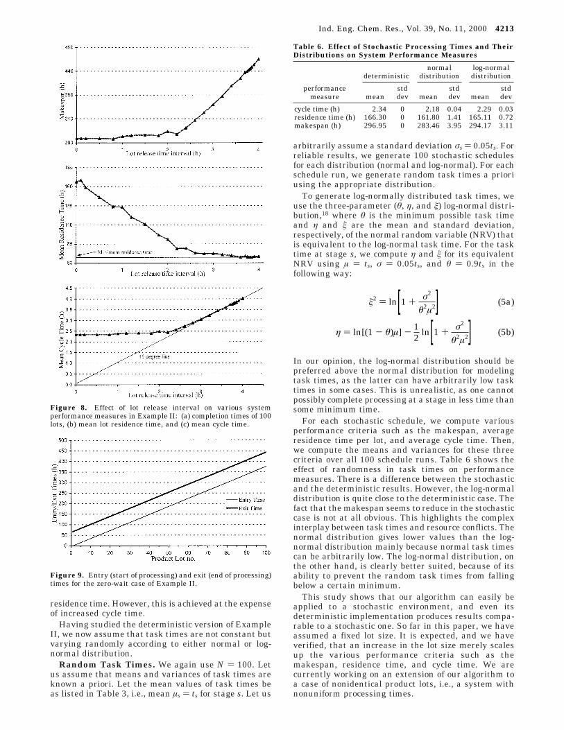
residence time. However, this is achieved at the expenseof increased cycle time.

Having studied the deterministic version of ExampleII, we now assume that task times are not constant butvarying randomly according to either normal or log-normal distribution.

Random Task Times. We again use N ) 100. Letus assume that means and variances of task times areknown a priori. Let the mean values of task times beas listed in Table 3, i.e., mean µs ) ts for stage s. Let us

arbitrarily assume a standard deviation σs ) 0.05ts. Forreliable results, we generate 100 stochastic schedulesfor each distribution (normal and log-normal). For eachschedule run, we generate random task times a prioriusing the appropriate distribution.

To generate log-normally distributed task times, weuse the three-parameter (θ, η, and ê) log-normal distri-bution,18 where θ is the minimum possible task timeand η and ê are the mean and standard deviation,respectively, of the normal random variable (NRV) thatis equivalent to the log-normal task time. For the tasktime at stage s, we compute η and ê for its equivalentNRV using µ ) ts, σ ) 0.05ts, and θ ) 0.9ts in thefollowing way:

In our opinion, the log-normal distribution should bepreferred above the normal distribution for modelingtask times, as the latter can have arbitrarily low tasktimes in some cases. This is unrealistic, as one cannotpossibly complete processing at a stage in less time thansome minimum time.

For each stochastic schedule, we compute variousperformance criteria such as the makespan, averageresidence time per lot, and average cycle time. Then,we compute the means and variances for these threecriteria over all 100 schedule runs. Table 6 shows theeffect of randomness in task times on performancemeasures. There is a difference between the stochasticand the deterministic results. However, the log-normaldistribution is quite close to the deterministic case. Thefact that the makespan seems to reduce in the stochasticcase is not at all obvious. This highlights the complexinterplay between task times and resource conflicts. Thenormal distribution gives lower values than the log-normal distribution mainly because normal task timescan be arbitrarily low. The log-normal distribution, onthe other hand, is clearly better suited, because of itsability to prevent the random task times from fallingbelow a certain minimum.

This study shows that our algorithm can easily beapplied to a stochastic environment, and even itsdeterministic implementation produces results compa-rable to a stochastic one. So far in this paper, we haveassumed a fixed lot size. It is expected, and we haveverified, that an increase in the lot size merely scalesup the various performance criteria such as themakespan, residence time, and cycle time. We arecurrently working on an extension of our algorithm toa case of nonidentical product lots, i.e., a system withnonuniform processing times.

Figure 8. Effect of lot release interval on various systemperformance measures in Example II: (a) completion times of 100lots, (b) mean lot residence time, and (c) mean cycle time.

Figure 9. Entry (start of processing) and exit (end of processing)times for the zero-wait case of Example II.

Table 6. Effect of Stochastic Processing Times and TheirDistributions on System Performance Measures

deterministicnormal

distributionlog-normaldistribution

performancemeasure mean

stddev mean

stddev mean

stddev

cycle time (h) 2.34 0 2.18 0.04 2.29 0.03residence time (h) 166.30 0 161.80 1.41 165.11 0.72makespan (h) 296.95 0 283.46 3.95 294.17 3.11

ê2 ) ln[1 + σ2

θ2µ2] (5a)

η ) ln[(1 - θ)µ] - 12

ln[1 + σ2

θ2µ2] (5b)


Conclusion

A simple one-pass algorithm based on a novel, product-at-a-time strategy was presented for scheduling a single-product process with reentrant flows and uniformprocessing times. The algorithm is well suited for waferfabs in semiconductor manufacturing, which demandcomplex scheduling considerations. Although developedwith a deterministic, zero-breakdown environment inmind, it can easily be extended to a stochastic, failure-prone environment, as illustrated in our paper. Usingthe concept of a rate-limiting stage, two lower boundson the time required to produce a number of lots werealso derived. Of these, one that is guaranteed is quiteconservative and works well for a small number of lots,whereas the other, which is not guaranteed, is quitegood for the scheduling of a large number of lots.Computationally, our algorithm performs far betterthan an existing partial enumeration method by Lee etal.10 Furthermore, it also gives much better makespansin almost all instances for the numerical example tested.The reentrant processes pose very challenging schedul-ing problems, and further work is in progress to enhanceand improve our algorithm and also to compare it withother simulation-based strategies employing queueprocessing rules.

Acknowledgment

This work was supported by a research grant(RP970642) from the National University of Singapore.We are indebted to Prof. M. P. Srinivasan for hisinvaluable discussions on the operation of wafer fabs.We also thank the reviewers for their constructivecomments that have led to a more complete paper. Inparticular, we thank the reviewer who commented ontask splitting.

Notation

Cik ) Completion time of task TikK ) Number of tasks in a product recipems ) Number of identical machines in stage sN ) Number of lots to be producedpk ) Processing time of task k in the recipesk ) Stage on which task Tk is performedS ) Total number of processing stages/stationsts ) Task processing time on stage st* ) Minimum cycle time of the system for a productt*last ) Cycle time of the last stage in a product recipeTk ) Task k in a product recipeTik ) Task k of product lot ivs ) Total number of visits made to stage s during a product

recipe

Greek Letters

µ ) Mean value of task timeσ ) standard deviation of task timeh ) Mean of the NRV equivalent to a log-normal RVê ) Standard deviation of the NRV equivalent to a log-

normal RVθ ) Minimum positive value of a log-normal random

variable

Abbreviations

SBA ) Sequence branch algorithmLB ) Lower bound

Literature Cited

(1) Seow, B. Q. Career in a DRAM wafer fab. In Proceedings ofthe interfaculty seminar on meeting the needs of the wafer fabs:Teaching of Microelectronis at NUS; Singapore, January 20, 1996;p 33.

(2) Srinivasan, M. P. A chemical engineer in the microelectron-ics industry. In Proceedings of the interfaculty seminar on meetingthe needs of the wafer fabs: Teaching of Microelectronis at NUS;Singapore, January 20, 1996; p 71.

(3) Wein, L. M. Scheduling semiconductor wafer fabrication.IEEE Trans. Semicond. Manuf. 1988, 1 (3), 115.

(4) Johri, P. K. Practical issues in scheduling and dispatchingin semiconductor wafer fabrication. J. Manuf. Syst. 1993, 12 (6),474.

(5) Kumar, P. R. Scheduling semiconductor manufacturingplants. IEEE Control Syst. Mag. 1994, 33.

(6) Kim, J. S.; Leachman, R. C. Decomposition method applica-tion to a large-scale linear programming WIP projection model.Eur. J. Oper. Res. 1994, 74, 152.

(7) Hung, Y. F.; Leachman, R. C. A production planningmethodology for semiconductor manufacturing based on iterativesimulation and linear programming calculations. IEEE Trans.Semicond. Manuf. 1996, 9 (2), 257.

(8) Dessouky, M. M.; Leachman, R. C. Dynamic models ofproduction with multiple operations and general processing times.J. Oper. Res. Soc. 1997, 48, 647.

(9) Lu, S. C. H.; Ramaswamy, D.; Kumar, P. R. Efficientscheduling policies to reduce mean and variance of cycle-time insemiconductor manufacturing plants. IEEE Trans. Semicond.Manuf. 1994, 7 (3), 374.

(10) Lee, S.; Bok, J. K.; Park, S. A new algorithm for large-scale scheduling problems: Sequence branch algorithm. Ind. Eng.Chem. Res. 1998, 37, 4049.

(11) Graves, S. C.; Meal, H. C.; Stefek, D.; Zeghmi, A. H.Scheduling of re-entrant flow shops. J. Oper. Manage. 1983, 3 (4),197.

(12) Peyrol, E.; Floquet, P.; Pibouleau, L.; Domenech, S.Scheduling and simulated annealing application to a semiconduc-tor circuit fabrication plant. Comput. Chem. Eng. 1993, 17 (S),S39.

(13) Ku, H. M.; Karimi, I. A. Completion time algorithms forserial multiproduct batch processes with shared storage. Comput-ers Chem. Eng. 1990, 14(1), 49.

(14) Applequist, G.; Samikoglu, O.; Pekny, J.; Reklaitis, G. V.Issues in the use, design and evolution of process scheduling andplanning systems. ISA Trans. 1997, 36 (2), 81.

(15) Kuriyan, K.; Reklaitis, G. V. Scheduling in networkflowshops. Comput. Chem. Eng. 1986, 36 (2), 81.

(16) Moon, S.; Park, S.; Lee, W. K. New MILP models forscheduling of multiproduct batch plants under zero-wait policy.Ind. Eng. Chem. Res. 1996, 35, 3458.

(17) Bhalla, A. Planning and scheduling of a thin film resistorprocess. M. Engg. Dissertation, National University of Singapore,Singapore, 2000.

(18) Johnson, N. L.; Kotz, S. Continuous Univariate Distribu-tions 1; Houghton Mifflin Company: Boston, MA, 1975.

Received for review April 3, 2000Revised manuscript received August 9, 2000

Accepted August 31, 2000

IE000380X


Documents

Scheduling a Single-Product Reentrant Process with Uniform Processing Times