Scheduling a two-machine robotic cell: A solvable case

Annals of Operations Research 57(1995)217-232 217

Scheduling a two-machine robotic cell: A solvable case

Eugene Levner

Department of Automated Systems, Centre for Technological Education, Affiliated with Tel-Aviv University, 52 Golomb St., Holon 58102( Israel

E-mail: msegen @ pluto.mscc.huji.ac.il

Konstantin Kogan

Department of Industrial Engineering, Tel-Aviv University, Ramat-Aviv, 69978 Tel-Aviv, Israel

Ilya Levin

Department of Automated Systems, Centre for Technological Education, Affiliated with Tel-Aviv University, 52 Golomb St., Holon 58102, Israel

The paper deals with the scheduling of a robotic cell in which jobs are processed on two tandem machines. The job transportation between the machines is done by a transportation robot. The robotic cell has limitations on the intermediate space between the machines for storing the work-in-process. What complicates the scheduling problem is that the loading/unloading operation times are non-negligible. Given the total number of operations n, an optimal O(n log n)-time algorithm is proposed together with the proof of optimality.

Keywords: Scheduling, robotic cell, tandem machines, optimization.

1. Introduction

Small-scale robotic cells with two tandem CNC machines for job processing and robots serving for transportation of jobs and tools are quite commonly found in real applications. They are the simplest automated blocks, the "islands of automation", in modem computer-integrated manufacturing. In order to efficiently utilize these automated facilities, diverse scheduling problems are to be solved (see, among others, Blazewicz et al. [2], Kusiak [5], Stecke and Suri [9]).

Since the introduction of the first analytical flowshop scheduling model by Johnson [3], a number of subsequent works on different versions of flowshop scheduling have appeared (see, for example, the surveys by Belen'kii and Levner [1] and Lawler et al. [6]). For recent examples, we can refer to the papers by Kise et al. [4], Stern

© J.C. Baltzer AG, Science Publishers

218 E. Levner et aL, Scheduling a two-machine robotic cell

and Vitner [10], and Panwalkar [8], in which they investigate robotic cells with limitations on the intermediate space between the machines for storing the work-in- process (WlP).

Kise et aI. [4] have considered a two-machine, one-robot, no-WIP-storage scheduling problem with a centralized storage and solved it efficiently. Another modification of the two-machine, one-robot flowshop scheduling problem, with job- dependent robot's transportation times has been considered by Stern and Vitner [10], who claimed the NP-hardness of the problem and suggested an approximate O(n log n)- time algorithm (n = the number of jobs to be processed).

Panwalkar [8] has considered another version of the no-WIP-storage cell configuration, with no space after the first machine for storing the completed jobs, but having the space for storing the WIP before the second machine, and has solved the problem in quadratic time using the Johnson algorithm as a subroutine. In the latter work, the loading/unloading operation times are assumed to be negligible and the transportation times are job independent.

In the present paper, we intend to study the two-machine robotic cell in the same geometric configuration as that in the Panwalkar [8] model. Proceeding from practical considerations, we complicate the model by allowing the loading/unloading operation times to be non-negligible.

In the following section, we describe the robotic cell that motivated this study and formulate the dynamics of the system. Then we describe the scheduling problem and its graph representation. Starting from the analysis of critical path properties in graphs, we suggest an O(n log n)-time algorithm for finding an optimal sequence that minimizes the completion time of n jobs, and prove its optimality. In conclusion, we refer to some possible directions for further research.

2. Description of the robotic cell

Consider the robotic cell that motivated this study. It is a component of the computer-integrated manufacturing system CIM-2000 MECHATRONICS produced by DEGEM SYSTEM, Ltd (Israel) which is up and running in the Holon Centre for Technological Education.

The cell contains two tandem CNC machines: milling machine Denford TRIAC VMC (machine MA), and lathe DEGEM NCL 2000 (machine MB). The cell also contains:

• one transporting robot DEGEM PS 2000 (robot TR);

• two robotic loaders, Mitsubishi HM01 (robots RA and RB);

• input automatic storage/retrieval station (AS/RS) for storing blanks and tools, and output AS/RS for storing finished parts, DEGEM ST-2000.

Cell configuration and capacity limitations of the input ASIRS do not allow it to be used for storing jobs completed on machine MA. At the same time, the output

E. Levner et al., Scheduling a two-machine robotic cell 219

AS/RS may be used for storing the jobs completed on MA; thus, the latter storage station serves as the integrated output-WIP AS/RS. The cell layout is depicted in figure 1.

MANAGEMENT STATION Input AS/RS MACHINE B

I !

Figure I. Layout of the robotic ceil.

At time zero, there are n jobs (parts) available in the input AS/RS; they are to be processed in turn on machines MA and MB.

The part's route in the cell is as follows: first, a due part is moved by the robot RA from the input AS/RS to machine MA; next, the transporting robot TR picks up the part finished on MA and delivers it to the output/WIP station where a stacker places the part into a predetermined cell, within the service range of robot RB. Next, RB loads the part on machine MB (if and when it is empty) and, after finishing the part on MB, puts the latter on the output AS/RS.

The problem is to schedule jobs on the machines so as to minimize the makespan M under the following standard restrictions:

(i) Every machine can perform at most one job at a time, and each job must be performed only on one machine at a time.

(ii) The same job sequence occurs on each machine.

(iii) The space of the output-WIP AS/RS is sufficiently large for storing all the required parts finished on MA.

The following non-standard conditions complicate the problem in comparison with the Johnson [3] and Panwalkar [8] flowshop models:

(1) the loading/unloading operation times are considered to be non-negligible, as is often the case in industry;

(2) the times for placing jobs into appropriate cells of the output-WIP storage are allowed to be job dependent.

220 E. Levner et al., Scheduling a two-machine robotic cell

3. Dynamics of the system

Let P = (Jr ..... Jn) be an arbitrary sequence of given jobs, where Jk stands for the kth job to be processed in the sequence. The jobs are processed in sequence P (the same on two machines) according to the following technological rules:

Rule

(a)

(b) (c)

(d)

1 (Controlling operations related to machine MA):

Robot RA starts its life cycle by taking the first job Jl from the input AS/RS and loading it on machine MA.

Next, machine MA starts processing job Jl.

After completing the processing of Jl on MA, transporting robot TR unloads the latter job from MA in order to move it to the WIP AS/RS before machine MB. Concurrently, robot RA starts its next life cycle by turning to the input AS/RS for the next job J2 scheduled to be processed.

Next, all other jobs J2 .... jn are loaded, processed on machine MA and unloaded by transporting robot TR, one after another. The unloading of job Jk, 2 < k < n, by robot TR starts either at the time when Jk is finished on MA, or at the time when TR returns to MA after delivering Jk-l to the MB's area, whichever is larger.

Rule 2 (Controlling the moves of the transporting robot):

(a) After job Jl is unloaded from MA, robot TR carries it from MA to the area of machine MB and places it into the output-WIP AS/RS.

(b) Immediately after that, TR moves back to machine MA.

(c) Concurrently, the stacker attached to the output-WIP AS/RS places job J l into a predetermined storage cell (within the service range of robot RB).

Other jobs J2 .... Jn are transported by TR and the stacker in a similar way; after delivering the last job, TR stops near the WIP AS/RS.

Rule 3 (Controlling operations related to machine MB):

(a) After job Jl is delivered by the stacker, robot RB (which originally waits in an initial position, near MB) reloads it to machine MB.

(b) After that, machine MB starts processing job Ji-

(c) After Jl is completed on MB, robot RB unloads it and delivers it to the output AS/RS. Then RB returns to its initial position, from where it starts its new life cycle by taking the next job from the WIP AS/RS (if and when it is available).

All other jobs j2 ..... Jn are performed on MB one after another, in a similar way as job Jl, until the last job is finished on MB and delivered to the output AS/RS.

E. Levner et aL, Scheduling a two-machine robotic cell 221

4. Mathematical description of the system

4.1. NOTATION

n = the given number of jobs;

For i = 1 ..... n:

La(i) = "loading time" for job i on machine MA (required to perform the job handling operations described in rule l(a));

PA(i) = processing time for job i on machine MA;

Ua(i ) = time required for robot TR to unload job i from MA;

Ln(i) and Pn(i) are, respectively, job-loading and processing times on machine MB (described above in rules 3(a) and 3(b));

Un(i) = time required for RB to unload job i from MB, deliver it to the output

AS/RS, and return to MB (see rule 3(c));

T = (job independent) travel time required for TR to move any job from MA to the WIP storage and drop it there;

R = "return time" required for robot TR to return from the WlP-output AS/RS to machine MA;

W(i) = "placement time" required for the stacker to place job i into the appropriate cell of the WlP storage.

Define also the key time instants of a schedule P = (Jl,J2 ..... Jn) as follows:

sa(i) : the time instant when RA starts its ith life cycle in P by turning from its initial position for loading job i on MA;

sB(i) : the time instant when robot RB starts its ith life cycle by reloading job i from the WIP storage to machine MB;

ua(i) : the time instant when TR starts unloading job i from MA;

fs(i) : the time instant when job i is released at the output AS/RS, that is, the completion time of servicing job i in the cell in the sequence P; i =Jl , J2 ..... Jn.

4.2. GRAPH PRESENTATION OF THE TECHNOLOGICAL PROCESS

The above technological process may be portrayed with the help of an oriented graph G(P) (see figure 2(a)), the arcs of which represent operations and precedence relations, and the nodes represent events occurring in time, that is, the moments of starting and finishing the operations. Operations duration are assigned to the corresponding arcs and called the arc lengths.

Node S of the graph denotes the start of processing of jobs and node F denotes the completion of the whole process.


Graph G(P)

~( j ) p ( j ) U (jl) LA(J 2) 5(J=) UA(i 2) L ( j) P(j ) U.(j ) ~ A z . A z . . . O A . : ~ ~ " = A ^ ":=,

L(Jl) PB (jl) U(Jl) LB(j=) PB(j=) U B (j2) Ls (j.) Pa (j.) Us (j.) (a)

a ' ( j ) 1

A b'(j 11 %==, v = v

Graph Z(P) a(j ) a(j )

2 ~ ~L n ~ 0 b d l h

(b) Figure 2. (a) Graph G(P) of the initial problem and (b) graph Z(P)

of the equivalent non-uniform (a, b, c) problem.

The thin-line arcs, called dummies, show precedence relations only and do not represent real operations; they have zero length. In particular, the dummies in figure 2 show that the jobs are to be processed on the machines in turn, one after another.

4.3. THE MAKESPAN AND CRITICAL PATHS

Given a sequence of n jobs, P = (Jl,J2 .... . Jn), the sa(i), sB(i), uA(i) andfB(i) values (where i =Jl,J2 .... . Jn) can be computed as follows.

According to rules l(a) and l(b),

sA( j l ) = O, uA( j l ) = LA( j l ) + PA(Jl). (1)

According to rules 1, 2(a) and 2(b),

s A ( j k ) = u A ( j k _ I ) + W a ( J k _ l ) , k = 2 . . . . . n,

uA( jk) = sA(jk) + max(T+ R, L~(jk) + PA(Jk)), k = 2 . . . . . n.

(2)


According to rules 2 and 3,

sB(jl) = ua(jl) + UA(jl ) + T + W(jl);

fB(jl) = sB(jl) + Ln(jl) + PB(Jl) + UB(jl);

SB(.~) = max(sS(A-l) + LB(A-1) + PB(.~-I) + UB(jk-l),

ua(jk) + UA(jk) + T + W(jk));

fS(jk) = sB(jk) + Ln(jk) + PB(A) + UB(jk), k = 2 ... . . n.

(3)

Note that if the loading/unloading times are negligible for all jobs, i.e. La(i) = Ua(i) = W(i) = 0 for all i, 1 < i < n, then the above relations (1)-(3) degenerate into those of the Panwalkar [8] model.

Denote by d an arbitrary directed path from S to F in graph G(P) and let L(d) be the length of d, the latter being defined as the sum of lengths of all arcs consti- tuting d.

It is well known in the literature (see, for example, Johnson [3], Kise et al. [4], Levner [7]) that in various scheduling problems the makespan M(P), for any fixed P, equal the length Lmax(P) of the critical (longest) path in G(P). The following lemma states that this fact is also valid for the problem considered.

LEMMA

For the considered two-machine scheduling problem,

M(P) = Lmax (P) = max L(d), (4) d~FI(P)

where I~(P) denotes the set of all directed paths from S to F in graph G(P).

The proof is by induction on n, using (1)-(3) and the fact that f~(jn) = M(P). It is omitted here as being similar to the proofs presented in Kise et al. [4] and Levner [7].

In the next section, we introduce an (a, b, c)-problem", which will serve below problem.

auxiliary flowshop problem, called "the to efficiently solve the initial scheduling

5. Analysis of scheduling problems

5.1. THE (a, b, c)-PROBLEM

Consider a two-machine, n-job Johnson-type problem in which processing each job is characterized by three parameters only (without any loading and transportation times whatsoever): a(i), b(i) and c(i). Two of these are the same as in the Johnson [3] problem:


a(i) = processing time of job i on machine MA.

b(i) = processing time of job i on machine MB,

while the third parameter is defined as follows:

c(i) = the minimal time interval that has to elapse between the start of processing job i on machine MA and the finish of processing that job on machine MB, i = 1,...,n.

Let us call this problem "the uniform (a, b, c)-problem". Its technological graph G is depicted in figure 3.

Graph G(Q)

a(j 1) a(j) a(k) a(j)

' ~ ) " ~" - - . = - = : - . . . - w ~ c(i)" ~"

(a)

Graph G(Q')

a(j~) a(k) a(j) a(J n)

(b) Figure 3. Graph G of the uniform (a, b, c)-problem for

two adjacent sequences, (a) Q and (b) Q'.

Together with the uniform (a, b, c)-problem, we shall also treat the so-called "non-uniform (a, b, c)-problem", obtained from the uniform (a, b, c)-problem as follows: for every job i, 1 < i < n, together with three numbers, a(i), b(i), and c(i) defined above, we are given three (generally speaking, other) time parameters a'(i), b'(i), c'(i) such that whenever job i is processed first in any sequence, it acquires new parameters a'(i), b'(i), c'(i), while all other jobs in the sequence possess the same a(i), b(i), and c(i) values as in the initial uniform (a, b, c)-problem. The main idea behind the definition is that in the algorithm below we will try each job with a'(i),


b'(i), and c'(i) values as an initial job, treating all other jobs as elements of a uniform (a, b, c)-problem. Graph Z(P), corresponding to a non-uniform (a, b, c)-problem, is depicted in figure 2(b).

5.2. OPTIMAL SOLUTION

The following theorem motivates introduction of the (a, b, c)-problem.

THEOREM 1

The initial n-job two-machine flowshop problem is reducible to an n-job non- uniform (a, b, c)-problem.

Proof Consider an arbitrary permutation of n jobs P and its corresponding graph

G(P) (see figure 2(a)). Let us construct an instance of the non-uniform (a, b, c)-problem equivalent

to the initial scheduling problem. For this purpose, we replace G(P) by an equivalent graph Z(P) corresponding to an (a, b, c)-problem (see figure 2(b)).

In order to make graphs G(P) and Z(P) equivalent, we define the auxiliary equivalent non-uniform (a, b, c)-problem as follows:

a'(i)

b '(i)

c'(i)

a(i)

b(i)

c(i)

= LA(i) + Pa(i) + Ua(i);

= Ls(i) + Ps(i) + UB(i);

= a '(i) + b'(i) + T + W(i);

= max(LA(i) + Pa(i); T+ R) + UA(i);

= LB(i) + es(i) + UB(i);

=a(i) + b(i) + T+ W(i), i=jl,j2,. . . , jn.

(5)

Due to (5), length Lmax(P) of the critical path from S to F in graph G(P) equals length Lmax(P) of the critical path from S to F in Z(P) as long as for each i, i =Jl ..... in, the following is valid:

(1) The length of the path leading from the beginning of the arc (operation) labelled La(i) to the end of the arc labelled UA(i) in G(P) equals the length (a'(i) or (a(i)) of the corresponding arc in Z(P).

(2) The length of the path leading from the beginning of arc (operation) LB(i) to the end of arc Us(i) in G(P) equals the length (b'(i) or b(i)) of the corresponding arc in Z(P).


(3) The length of the path leading from the beginning of arc (operation) LA(i) to the end of arc UB(i) in G(P) equals the length (c'(i) or c(i)) of the corresponding arc in Z(P) (see figures 2(a, b)).

Then, taking (4) into account, we obtain that the makespan M(P) is the same for both problems. Therefore, the minimal makespan for the described (a, b, c)- problem will provide, at the same time, the minimal makespan for the original scheduling problem. []

The following theorem shows that the n-job uniform (a, b, c)-problem is solvable in polynomial time.

THEOREM 2

A sequence for the two-machine uniform (a, b, c)-problem is optimal whenever first the jobs i for which a(i)< b(i) are processed, arranged so that the c ( i ) - b(i) values are ordered from the smallest to the largest, and these jobs are followed by the remaining ones (i.e. such that a(i) > b(i)) arranged so that the c(i) - a(i) values are ordered from the largest to the smallest.

Proof

Let P* be the sequence in which jobs are arranged according to the rule formulated in the theorem, and assume that it is not optimal. Then there exists an optimal sequence, say Q, containing two jobs, say j and k, with j immediately preceding k, for which the condition of the theorem does not hold.

The latter circumstance is possible in the following cases:

(i) a( j ) < b(j), a(k) < b(k), and c(j) - b(j) > c(k) - b(k);

(ii) a( j ) > b(j) , a(k) > b(k), and c( j) - a( j ) < c(k) - a(k);

(iii) a( j ) > b(j) , and a(k) < b(k).

Due to the above assumption on the optimality of Q,

M(Q) < M(P*). (6)

Consider the sequence Q ' = (... k, j . . . ) , obtained from Q by interchanging jobs j and k. We intend to show that Q' is not worse that Q, that is M(Q' ) < M(Q). For this purpose, we will use equation (4) as related to the considered (a, b, c)- problem and to its graph depicted in figure 3.

Compare the critical paths in graphs G(Q) and G(Q') (see figure 3), and show that for all the above cases (i)-(iii), the critical path in G(Q') is not larger than the critical path in G(Q), or

max(c(k) + b(j), a(k) + c(j)) < max(c(j) + b(k), a(j) + c(k)). (7)


1. Let case (i) take place. Since c(k) + b( j ) < c( j ) + b(k), and a( j ) <_ b(j), then a( j ) + c(k) <_ c(k) + b( j ) < c( j ) + b(k), and therefore max(c(j) + b(k), a ( j ) + c(k)) = c( j ) + b(k).

Consider two subcases:

( la) If max(c(k) + b( j ) , a(k) + c ( j ) ) = c(k) + b ( j ) (that is, c(k) + b ( j ) >_ a(k) + c(j)), then by virtue of c( j ) - b ( j ) > c(k) - b(k), we have that c( j ) + b(k) > c(k)+ b( j ) and, therefore, (7) holds.

( lb) If max(c(k) + b( j ) , a(k) + c ( j ) ) = a(k) + c( j ) (that is, c(k) + b ( j ) <_ a(k) + c(j)), then by virtue of a(k) <_ b(k), we have that c( j ) + b(k) >_ a(k) + c( j ) and, therefore, in case (i) inequality (7) holds.

2. Let case (ii) take place. Since a( j ) + c(k) > a(k) + c(j) and a( j ) > b(j) , then a( j ) + c(k) > a(k) + c( j ) > c(j) + b(k), and therefore max(c(j) + b(k), a ( j ) + c(k)) = a ( j ) + c(k). Consider two subcases:

(2a) If max(c(k) + b(j), a(k) + c(j)) = c(k) + b( j ) then by virtue of a(j) > b(j), we have that a( j ) + c(k) > c(k) + b( j ) and, therefore, inequality (7) holds.

(2b) If max(c(k) + b( j ) , a(k) + c( j ) ) = a(k) + c( j) , then by virtue of c( j ) - a( j ) < c(k) - a(k), we have that a( j ) + c(k) > a(k) + c( j ) and, therefore, in case (ii) inequality (7) holds.

3. Let case (iii) take place. Consider four subcases:

(3a) max(c(k) + b(j), a(k) + c( j ) ) = c(k) + b(j) , and

max(c(j) + b(k), a( j ) + c(k)) = c( j ) + b(k).

In this subcase, by virtue of a( j ) > b(j) , we have that c( j ) + b(k) > a( j ) + c(k) > b( j ) + c(k), that is, (7) holds.

(3b) max(c(k) + b(j), a(k) + c( j)) = c(k) + b(j) , and

max(c(j) + b(k), a ( j ) + c(k)) = a( j ) + c(k).

In this subcase, by virtue of a( j ) > b(j), we have that c(k) + b( j ) < c(k) + a(j) , that is, (7) holds.

(3c) max(c(k) + b(j), a(k) + c( j ) ) = a(k) + c(j) , and

max(c(j) + b(k), a ( j ) + c(k)) = c( j ) + b(k).

By virtue of a(k) <_ b(k), we have that a(k) + c( j ) <_ b(k) + c(j) , that is, (7) holds.

(3d) max(c(k) + b(j), a(k) + c( j ) ) = a(k) + c(j) , and

max(c(j) + b(k), a( j ) + c(k)) = a( j ) + c(k).

By virtue of a(k) <_ b(k), we have that a( j ) + c(k) >_ c( j ) + b(k) > c( j ) + a(k), that is, in case (iii) inequality (7) holds.


By virtue of (7), we can conclude that the critical path in G(Q') is not larger than the critical path in G(Q), and taking (4) into account, we derive that the makespan cannot increase in reversing the order of jobs j and k: M ( Q ' ) < M(Q).

If Q ' = P*, we have a contradiction to (6). If Q" ~: P*, we may find in Q ' a new pair of jobs, say I and m, with l immediately

preceding m, for which the condition of the theorem does not hold. Consider the sequence Q" = ( . . . m, l . . . ), obtained from Q' by interchanging jobs l and m. Applying again the above arguments, we derive: M(Q") < M(Q') . After a finite number of such pairwise interchanges, sequence P* can be obtained from Q, with M(P*) < ... < M(Q") < M ( Q ' ) < M(Q). This is a contradiction to (6), which completes the proof. []

The following corollaries can be easily derived.

COROLLARY 1

The n~ob u n i ~ r m (a, b, c)-problem is solvable in O(n log n) time.

COROLLARY 2

Consider the n-job non-uniform (a, b, c)-problem defined above, and let a certain job, say i, be specified as the first one in any schedule. Then, if the remaining jobs { 1 ..... n } \ i are arranged in the same order as they appear in the optimal solution of the initial n-job uniform (a, b, c)-problem (that is, according to the rule stated in theorem 2), we shall obtain an optimal sequence for the non-uniform (a, b, c)-problem considered.

Based on the above analysis, we can now describe an algorithm for solving the initial scheduling problem.

6. Sequencing algorithm

6.1.

Input: Output:

Step 1.

ALGORITHM DESCRIPTION

For all i, 1 < i < n, LA(i), Pa(i), Ua(i), LB(i), PB(i), Us(i), T, R, and W(i).

An optimal solution P* of the initial n-job, two-machine problem, and the minimal makespan M* = M(P*) = mineM(P).

[Define the auxiliary uniform and non-uniform (a, b, c)-problems]. Let

a'(i) = LA (i) + P3 (i) + UA (i);

c'(i) = a'(i) + b'(i) + T + W(i);

b(i) = LB(i) + PB(i) + UB(i);

b'(i) = LB(i) + PB(i) + UB(i);

a(i) = max(L A (i) + PA (i), T + R) + U A (i);

c(i) = a(i) + b(i) + T + W(i); i = 1 . . . . . n.


Step 2.

Step 3.

Step 4.

[Find an optimal sequence for the uniform (a, b, c)-problem].

Arrange first the jobs i for which a(i)<_ b(i), in non-decreasing order of c ( i ) - b(i) values, and then arrange the remaining jobs in non-increasing order of c(i) -a ( i ) values. Denote the sequence obtained by p0 = ( jo , jo . . . . . jo ) ; M 0 = M(po).

[Try each job i as an initial, with all the remaining jobs being arranged as in p0].

Move job i = j ° (2 < k < n) in p0 to the first position and shift the first k - 1 jobs one position to the right; denote the sequence obtained by Pk, 2 < k < n. Take p0 as Pl- Calculate the makespan Mk = M(Pk) for each of the obtained sequences Pk, 1 < k < n.

[Find the minimal makespan and an optimal sequence].

F ind M * = minlsk~nM(Pk); then M* is the min ima l makespan and P * = arg minkM(Pk) is an optimal sequence.

6.2. ALGORITHM COMPLEXITY

Let us verify that the algorithm described above runs in O(n log n) time. In step 1, in order to determine the auxiliary uniform and non-uniform (a, b, c)-

problems, we need O(n) operations. In step 2, in order to find the optimal sequence pO for the uniform (a, b, c)-

problem, we need O(n log n) time (see corollary 1). Let us show that O(n) t ime is sufficient to run step 3. Given p0, let us introduce, for each i, i = 1 ..... n, six auxiliary parameters,

which we call "potentials". In order to simplify the notation, let us re-enumerate the jobs so that p0 = (1, 2,. . . , n). The potentials for this p0 are defined as follows:

pO)(k) = p(2)(k) = O, for k = 1;

k - 1 k - 1

p(1) (k) = E a(i); p(2)(k) = E b(i), for 2 _< k __. n; i = I i = l

p(3)(k) = the makespan (i.e. the completion time) to fulfill jobs 1, 2 .... . k - 1 on two machines in this order, 2 < k _< n;

p(4)(k) = p(5) (k) = 0, for k = n;

tl n

p(4)(k) = ~ a(i); p(5)(k) = ~ b(i), for 1 < k < n - 1; i = k + l i = k + l

p(6)(k) = the makespan to fulfill jobs k + 1, k + 2 .. . . . n on two

machines in this order, k = 1 .. . . . n - 1.


Potentials p(3)(k) and p(6)(k) can be calculated recursively as follows:

p(3) (1) = O, p(3) (2) = max(b(1), c(1));

pC3)(k) = max(pO)(k)+c(k- 1), p(3)(k - 2 ) + b ( k - 1)), for k = 3 . . . . n;

p(6) (n) = 0, p(6) (n - 1) = max(a (n) , c(n));

p(6)(k) = max(p(5) (k ) + c(k + l), pt6) (k + 2 ) + a(k + l)), for k = n - 2,n - 3 .. . . . 1.

The above formulas show that O(n) t ime is sufficient for finding all the potentials. The main idea behind the definition of potentials is that, for each k, 1 < k < n, they permit us to determine the makespan M(Pk) in O(1) time.

Indeed, consider sequence Pk in the corresponding non-uniform (a, b, c)-problem treated in step 3, and aggregate the jobs appearing before job i = k (k = 2 ..... n) in p0 into an equivalent "job" Jk having the following a, b, c-parameters:

a(jk ) = pO) (k); b(J k ) = p(2) (k); c(J k ) = p(3) (k).

In a similar way, aggregate the jobs appearing after job i = k (k = 1,..., n - 1) in p0 into an equivalent "job" jk having the following parameters:

a( j k ) = p(4) (k); b(J k ) = p(5) (k); c(J k ) = p(6) (k).

Consider now a sequence Pk as a sequence of three jobs: i = k (standing in the first position), Jk and jk: Pk = (k, Jk, jk).

The makespan M(Pk) due to (4), for any fixed i = k, can be calculated in O(1) time: M(Pk) = max(a ' (k ) + a(Jk) + a(Jk), a'(k) + a(Jk) + c(Jk), a'(k) + C(Jk) + b(Jk), c'(k) + bUk) + bU~), b'(k) + b(Jk) + bUk)).

Therefore, in order to calculate all n makespan values in step 3, we need O(n) operations.

Step 4 requires O(n) operations. Hence, O(n log n) time is sufficient to optimally solve the scheduling problem

considered.

Remark

As we have mentioned above, the problem considered is a generalization of the Panwalkar problem; hence, incorporating the above potentials into the (quadratic) Panwalkar [8] algorithm, we can derive a modification of the latter running in O(n log n) time.

7. A numerical example

In the following example, travel times T and R equal 5 units and loading times LA(i), Lt~(i), Us(i) are zero for all i, 1 < i < n. The other parameters (processing


Table 1

Input parameters of the initial problem.

Job PA(i) Ps(i) W(i) UA(i )

1 12 24 18 23

2 20 33 8 7

3 15 35 10 3

4 5 10 12 15

5 I 5 3 1

6 18 13 17 12

7 10 25 11 13

Table 2

Parameters of the (a, b, c)-problems.

Job a(O b(i) c(i) a'(i) b'(i) c'(i)

1 35 24 82 35 24 82

2 27 33 73 27 33 73

3 18 35 68 18 35 68

4 25 I0 52 20 10 47

5 11 5 24 2 5 15

6 30 13 65 30 13 65

7 23 25 64 23 25 64

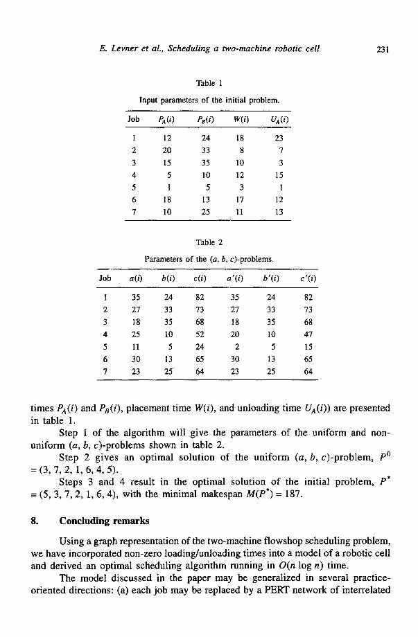
times Pa(i) and PB(i), placement time W(i), and unloading time UA(i)) are presented in table 1.

Step 1 of the algorithm will give the parameters of the uniform and non- uniform (a, b, c)-problems shown in table 2.

Step 2 gives an optimal solution of the uniform (a, b, c)-problem, p0 = (3 ,7 ,2 , 1 ,6,4,5) .

Steps 3 and 4 result in the optimal solution of the initial problem, P* = (5, 3, 7, 2, 1, 6, 4), with the minimal makespan M(P*) = 187.

8. Concluding remarks

Using a graph representation of the two-machine flowshop scheduling problem, we have incorporated non-zero loading/unloading times into a model of a robotic cell and derived an optimal scheduling algorithm running in O(n log n) time.

The model discussed in the paper may be generalized in several practice- oriented directions: (a) each job may be replaced by a PERT network of interrelated


operations; (b) the transporting robot may be used for delivering tools and fixtures, with delivery times being job dependent; (c) more than one transporting robot and more than two machines may be treated; (d) the limited capacity o f the output-WIP AS/RS may not be sufficient for storing all the required WIPjobs . To the best of our knowledge, under assumptions (a) and (b) the scheduling problem retains the property o f polynomial solvability, while in cases (c) and (d) it becomes NP-hard.

References

[1] A.S. Belen'kii and E.V. Levner, Scheduling models and methods in optimal freight transportation planning, Auto. Remote Contr. 10(1991)1-56.

[2] T. Blazewicz, G. Finke, R. Haupt and G. Schmidt, New trends in machine scheduling, Euro. J. Oper. Res. 37(1988)303-317.

[3] S.M. Johnson, Optimal two- and three-stage production scheduling with setup times included, Naval. Res. Log. Quart. I(1954)61-68.

[4] H. Kise, T. Shioyama and T. Ibaraki, Automated two-machine flowshop scheduling: A solvable case, l ie Trans. 23(1991)10-16.

[5] A. Kusiak, Scheduling flexible machining and assembly systems, in: Flexible Manufacturing Systems. Operations Research Models and Applications, ed. K.E. Stecke and R. Suri (Elsevier, New York, 1986) pp. 521-532.

[6] E.L. Lawler, J.K. Lenstra, A.H.G. Rinnooy Kan and D.B. Shmoys, Sequencing and scheduling: Algorithms and complexity, in: Logistics of Production and Inventory, Handbooks in Operations Research and Management Science, Vol. 4, ed. S. Graves, A. Rinnooy Kan and P. Zipkin (North- Holland, New York, 1993).

[7] E.V. Levner, Optimal planning of part's machining on a number of machines, Auto. Remote Contr. 11 (1969) 1972-1979.

[8] S.S. Panwalkar, Scheduling of a two-machine flowshop with travel time between machines, J. Oper. Res. Soc. 42(1991)609-613.

[9] R.E. Stecke and R. Suri (eds.), Flexible Manufacturing Systems: Operations Research Models and Applications (Elsevier, New York, 1986).

[10] H.I. Stern and G. Vitner, Scheduling parts in a combined production-transportation work cell, J. Oper. Res. Soc. 41(1990)625-632.

Documents

Scheduling a two-machine robotic cell: A solvable case