Embed Size (px)
Citation preview

Information Sciences 189 (2012) 282–292
Contents lists available at SciVerse ScienceDirect
Information Sciences
journal homepage: www.elsevier .com/locate / ins
Scheduling problems with two agents and a linear non-increasingdeterioration to minimize earliness penalties
Yunqiang Yin a,b, Shuenn-Ren Cheng c, Chin-Chia Wu d,⇑a State Key Laboratory Breeding Base of Nuclear Resources and Environment, East China Institute of Technology, Nanchang 330013, Chinab School of Sciences, East China Institute of Technology, Fuzhou, Jiangxi 344000, Chinac Graduate Institute of Business Administration, Cheng Shiu University, Kaohsiung County, Taiwand Department of Statistics, Feng Chia University, Taichung, Taiwan
a r t i c l e i n f o
Article history:Received 31 January 2011Received in revised form 1 November 2011Accepted 26 November 2011Available online 3 December 2011
Keywords:SchedulingSingle-machineTwo agentsDeterioration
0020-0255/$ - see front matter � 2011 Elsevier Incdoi:10.1016/j.ins.2011.11.035
⇑ Corresponding author.E-mail address: [email protected] (C.-C. W
a b s t r a c t
We consider a scheduling environment with two agents and a linear non-increasing dete-rioration. By the linear non-increasing deterioration we mean that the actual processingtime of a job belonging to the two agents is defined as a non-increasing linear functionof its starting time. Two agents compete to perform their respective jobs on a common sin-gle machine and each agent has his own criterion to be optimized. The goal is to schedulethe jobs such that the combined schedule performs well with respect to the measures ofboth agents. Three different objective functions are considered for one agent, includingthe maximum earliness cost, total earliness cost and total weighted earliness cost, whilekeeping the maximum earliness cost of the other agent below or at a fixed level U. We pro-pose the optimal (nondominated) properties and present the complexity results for theproblems addressed here.
� 2011 Elsevier Inc. All rights reserved.
1. Introduction
Recent developments in the field of distributed decision making have triggered a growing interest towards multi-agentscheduling problems, i.e., in which different agents share a common processing resource, and each agent wants to minimizea cost function depending on its jobs only. A number of papers investigate the two-agent setting. Baker and Smith [4] ana-lyzed the computational complexity of combining the agents’ criteria into a single objective function in a scenario with twoagents and various criteria (maximum completion time, total weighted completion time and maximum lateness). Agnetiset al. [1,2] addressed both the problems of finding a single Pareto-optimal solution and enumerating the whole set ofPareto-optimal solutions for different machine settings, under three different criteria: maximum of a regular function (suchas makespan or lateness), weighted total completion time, and number of tardy jobs. They studied the nine problems arisingfrom the different criteria combinations for the two agents, and stated complexity results for most of the resulting cases.Cheng et al. [7,8] provided further complexity and approximation results for some special cases, namely when the twoagents wish to minimize the weighted number of tardy jobs and the case in which they both hold max-form objective func-tions. Ng et al. [26] considered a two-agent scheduling problem on a single machine, where the objective is to minimize thetotal completion time of the first agent with the restriction that the number of tardy jobs of the second agent cannot exceed agiven number. They showed that the problem is NP-hard under high multiplicity encoding and can be solved in pseudo-polynomial time under binary encoding. When the first agent’s objective is to minimize the total weighted completion time,
. All rights reserved.
u).
Y. Yin et al. / Information Sciences 189 (2012) 282–292 283
they showed that the problem is strongly NP-hard even when the number of tardy jobs of the second agent is restricted to bezero. Lee et al. [16] focused on minimizing the total weighted completion time, and introduced fully polynomial-timeapproximation schemes and an efficient approximation algorithm with a reasonable worst case bound. Lee et al. [17,18] con-sidered a two-machine flowshop setting with two agents and they proposed a branch-and-bound algorithm and a simulatedannealing heuristic algorithm to search for the optimal solution and near-optimal solutions, respectively. Wan et al. [31]considered several two-agent scheduling problems with controllable job processing times, where agents A and B have toshare either a single machine or two identical machines in parallel while processing their jobs. Mor and Mosheiov [24] con-sidered the scheduling problems with two competing agents to minimize the minmax and minsum earliness measures. Spe-cifically, they focused on minimizing the maximum earliness cost or total (weighted) earliness cost of one agent, subject toan upper bound on the maximum earliness cost of the other agent. They introduced a polynomial-time solution for the min-max problem, and proved NP-hardness for the weighted minsum case. Liu et al. [22] introduced a new scheduling model inwhich two agents and increasing linear deterioration exist simultaneously. They studied two scheduling problems with thedifferent combinations of two agents’ objective functions: makespan, maximum lateness, maximum cost and total comple-tion time, and they proposed the optimal properties and presented the optimal polynomial time algorithms to solve thescheduling problems, respectively. Two-agent group scheduling with deteriorating jobs on a single machine was studiedin Liu et al. [21].
On the other hand, machine scheduling problems with a time-dependent deterioration have received increasing attentionin recent years. Researchers have formulated this phenomenon into different models and solved different versions of theproblem for various criteria. Generally, there are two types of models describing this kind of processes. The first type is de-voted to the problems in which the job processing time is characterized by a non-decreasing function, and the second typeconcerns problems in which the job processing time is given by a non-increasing function. For the second type of problems,i.e., single-machine scheduling problems with a non-increasing deterioration, Ho et al. [11] assumed that the actual process-ing time of job Jj is pj = aj(1 � kt) if it is scheduled at time t, where aj is the normal processing time of job Jj and k P 0 is a
constant such that k t0 þPn
j¼1aj � amin
� �< 1 in which amin = minj=1,2,. . .,n{aj}. Similar model was further studied in Ng et al.
[25], Wang [32], Wang and Xia [39], and so on. For research results on other scheduling models with a time-dependent dete-rioration, the readers can refer to Alidaee and Womer [3], Cheng et al. [6,9], Hsu et al. [12], Inderfurth et al. [13], Janiak andKovalyov[14], Kuo and Yang [15], Lee and Lai [19], Li et al. [20], Mazdeh et al. [23], Wang and Cheng [33], Wang and Wei [38],Wang et al. [34–37], Wu et al. [40], Yang and Yang [42], Yin et al. [41], Zhao and Tang [43,44], and Zhao et al. [45], etc.
Meanwhile, in real industrial systems the completion of jobs before their due date could result in additional storage orinsurance costs, or even product deterioration. In order to avoid holding costs, it is reasonable to consider the earliness pen-alty minimization. For more real world applications, we refer readers to Balin [5], Pan et al. [27], Qi and Tu [28], Shabtay [29],Valente [30], and Wang et al. [35]. In this paper we introduce a new scheduling model in which both two agents and a linearnon-increasing deterioration exist simultaneously. Specifically, the objective functions we consider in this paper are themaximum earliness cost, total earliness cost and total weighted earliness cost. We propose the optimal (nondominated)properties and present the optimal polynomial time algorithms to solve the scheduling problems addressed here.
The remainder of this paper is organized as follows. In Section 2, the notation and the terminology used throughout thepaper are introduced. In Sections 3–5, the complexity of several decision problems is characterized and studied. Someconclusions are given in the last Section.
2. Model formulation
Suppose that there are two competing agents, called agent A and agent B, each of them has a set of non-preemptive jobs tobe processed on a common machine. All jobs are available for processing at time t0, where t0 P 0. The agent A has to execute
the job set J A ¼ J A1 ; J
A2 ; . . . ; J A
nA
n o, whereas agent B has to execute the job set JB ¼ JB
1 ; JB2 ; . . . ; JB
nB
n o. Let X 2 {A,B}. The jobs belong-
ing to agent X are called X-jobs. The normal processing time, due-date and weight of job J Xj in the set J X are denoted by aX
j ; dXj
and wXj ðj ¼ 1;2; . . . ;nXÞ, respectively.
As commonly assumed in scheduling problems involving earliness, we restrict all the jobs to be completed prior to a pre-specified common deadline, otherwise we trivially schedule all the jobs sufficiently late to have no earliness cost. Thus, let Ddenote the common deadline of all the jobs with D P
PJ Xj 2J A[JB aX
j .
We say that a schedule S is nondominated if there is no schedule S0 such that f A(S0) 6 A(S), f B(S0) 6 f B(S) and at least one ofthe two inequalities is strict, i.e., a schedule is nondominated if a better schedule for one of the two agents necessarily resultsin a worse schedule for the other agent.
Following Ho et al. [11], we assume that the actual processing time pXj of job J X
j is a non-increasing linear function of itsstarting time, i.e.,
pXj ¼ aX
j ð1� ktÞ; j ¼ 1;2; . . . ;nX ;
where t P t0 is its starting time and k P 0 is a constant such that k t0 þP
J Xj 2J A[JB aX
j � amin
� �< 1 in which
amin ¼minJ Xj 2J A[JBfaX
j g.

284 Y. Yin et al. / Information Sciences 189 (2012) 282–292
Let S be a feasible schedule of the n = nA + nB jobs, i.e., a feasible assignment of starting times to the jobs of both agents.
The completion time of job J Xj is denoted as C X
j ðSÞ and the earliness of job J Xj is given by EX
j ðSÞ ¼max 0; dXj � C X
j ðSÞn o
. We shall
write C Xj and EX
j for C Xj ðSÞ and EX
j ðSÞ, respectively, whenever this does not generate confusion. For each job J Xj , let f X
j ð�Þ be a
non-decreasing function. In this case, we define the maximum earliness cost f Xmax ¼maxj¼1;2;...;nX f X
j ðEXj Þ
n ofor agent X. The
objective function of agent X takes one of the following three forms: f Xmax (maximum earliness cost),
PEX
j (total earliness
cost) andP
wXj EX
j (total weighted earliness cost).In the sequel, we will adopt the three-field notation scheme ajbjc introduced by Graham et al. [10] to denote the consid-
ered problems in this paper. We consider the following three objectives: 1jpXj ¼ aX
j ð1� ktÞjf Amax : f B
max 6 U; 1jpXj ¼ aX
j ð1� ktÞ;dA
j ¼ dAjP
EAj : f B
max 6 U and 1jpXj ¼ aX
j ð1� ktÞ; dAj ¼ dAj
PwA
j EAj : f B
max 6 U.
3. Problem 1jpXj ¼ aX
j ð1� ktÞjf Amax : f B
max <U
In this section, we address the problem of finding an optimal (nondominated) solution for1jpX
j ¼ aXj ð1� ktÞjf A
max : f Bmax 6 U. We show that this problem can be efficiently solved in a polynomial time. Before presenting
the algorithm, we first propose several optimal properties of the problem.
Lemma 3.1. For a given schedule S ¼ JX1½1� ; J
X2½2� ; . . . ; JXn
½n�
� �for the problem 1jpX
j ¼ aXj ð1� ktÞjCmax, if job JX1
½1� starts at time t0, then the
completion time of job JXh½h� ðh ¼ 1;2; . . . ;nÞ is equal to
t0 �1k
� �Yh
j¼1
1� kaXj
½j�
� �þ 1
k;
where Xj 2 {A,B}, and aXj
½j� is the normal processing time of the job JXj
½j� scheduled in jth position in S.
Proof. It is straightforward by induction. h
Proposition 3.2. Consider a feasible instance of 1jpXj ¼ aX
j ð1� ktÞjf Amax : f B
max 6 U, there is an optimal schedule in which the first
job starts at time t0 such that t0 � 1k
� �Qhj¼1 1� ka
Xj
½j�
� �þ 1
k ¼ D, and there are no idle times between consecutive jobs.
Proof. Note that both the objective functions f Amax and f B
max are non-increasing functions of the completion time. Hence thejobs will be processed as late as possible (subject to their common deadline constraint), and so there is no convenience inkeeping the machine idle. h
Proposition 3.3. Assume that the last scheduled job (so far) is completed at time t. If there is a B-job JBj such that
f Bj maxf0; dB
j � ðt þ aBj ð1� ktÞÞg
� �6 U, then there is an optimal schedule in which a B-job is scheduled at time t and there is
no optimal schedule in which an A-job is scheduled at time t.
Proof. Consider an optimal schedule S where the B-job JBh such that f B
h max 0; dBh � ðt þ aB
hð1� ktÞÞn o� �
6 U is not scheduledat time t. Let J X
l be the job scheduled at time t, where X 2 {A,B}. In this sequence, job JBh is scheduled later than time t. Let p
denote the set of jobs scheduled after job J Xl and prior to job JB
h , and let p0 denote the set of jobs scheduled after job JBh . We
create from S a new schedule S0 by extracting job JBh , reinserting it just before job J X
l and leaving the other jobs unchanged in S.
We claim that schedule S0 is still feasible and optimal. Note first that the completion time of each job processed before job J Xl
in S is not affected. By Lemma 3.1, the completion time of job JBh in S is equal to that of the last job scheduled in the subse-
quence p of S0, and so the completion time (and hence the earliness cost) of each job in p0 is identical in both S and S0. More-over, each job in p is scheduled later in S0, implying that its completion time is later in S0 by Lemma 3.1, and hence its
earliness cost is not larger in S0, i.e., f Yj EY
j ðS0Þ
� �6 f Y
j EYj ðSÞ
� �for any job JY
j in p, where Y 2 {A,B}, as required. h
Proposition 3.4. Assume that the last scheduled job (so far) is completed at time t. If for any unscheduled B-job
JBj ; f B
j max 0; dBj � ðt þ aB
j ð1� ktÞÞn o� �
> U, then there is an optimal schedule in which the A-job from the unscheduled A-jobs
with the minimum earliness cost is scheduled at time t.
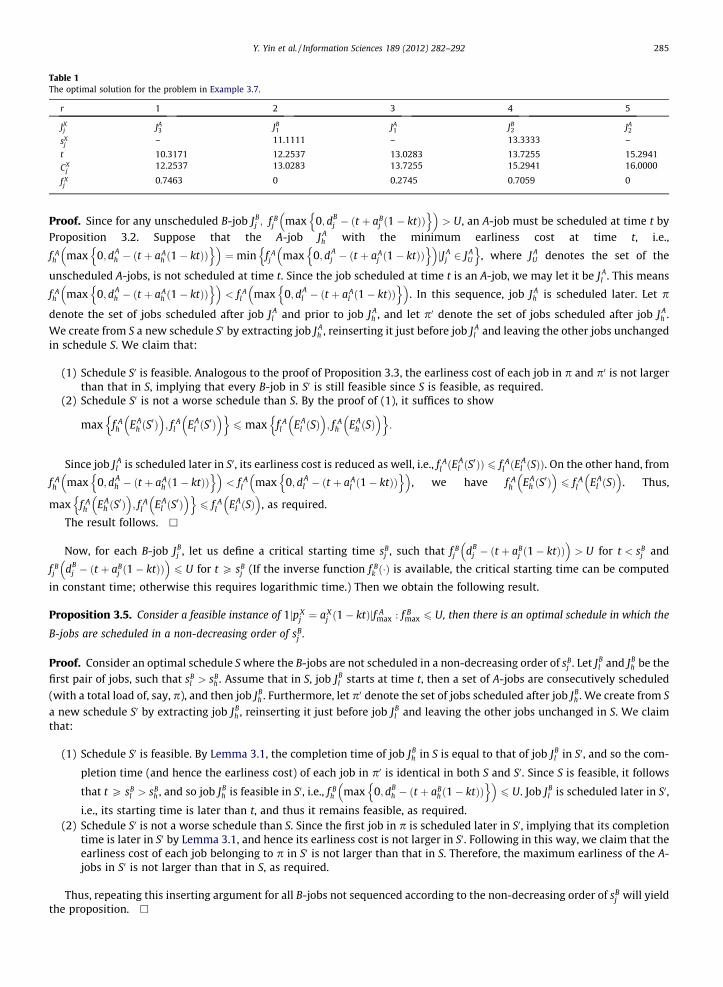
Table 1The optimal solution for the problem in Example 3.7.
r 1 2 3 4 5
JXj JA
3 JB1 JA
1 JB2 JA
2
sXj
– 11.1111 – 13.3333 –
t 10.3171 12.2537 13.0283 13.7255 15.2941
CXj
12.2537 13.0283 13.7255 15.2941 16.0000
f Xj
0.7463 0 0.2745 0.7059 0
Y. Yin et al. / Information Sciences 189 (2012) 282–292 285
Proof. Since for any unscheduled B-job JBj ; f B
j max 0; dBj � ðt þ aB
j ð1� ktÞÞn o� �
> U, an A-job must be scheduled at time t byProposition 3.2. Suppose that the A-job J A
h with the minimum earliness cost at time t, i.e.,
f Ah max 0; dA
h � ðt þ aAh ð1� ktÞÞ
n o� �¼min f A
j max 0; dAj � ðt þ aA
j ð1� ktÞÞn o� �
jJ Aj 2 J A
U
n o, where J A
U denotes the set of the
unscheduled A-jobs, is not scheduled at time t. Since the job scheduled at time t is an A-job, we may let it be J Al . This means
f Ah max 0; dA
h � ðt þ aAh ð1� ktÞÞ
n o� �< f A
l max 0; dAl � ðt þ aA
l ð1� ktÞÞn o� �
. In this sequence, job J Ah is scheduled later. Let p
denote the set of jobs scheduled after job J Al and prior to job J A
h , and let p0 denote the set of jobs scheduled after job J Ah .
We create from S a new schedule S0 by extracting job J Ah , reinserting it just before job J A
l and leaving the other jobs unchangedin schedule S. We claim that:
(1) Schedule S0 is feasible. Analogous to the proof of Proposition 3.3, the earliness cost of each job in p and p0 is not largerthan that in S, implying that every B-job in S0 is still feasible since S is feasible, as required.
(2) Schedule S0 is not a worse schedule than S. By the proof of (1), it suffices to show
max f Ah E A
h ðS0Þ
� �; f A
l EAl ðS
0Þ� �n o
6 max f Al E A
l ðSÞ� �
; f Ah EA
h ðSÞ� �n o
:
Since job J Al is scheduled later in S0, its earliness cost is reduced as well, i.e., f A
l ðEAl ðS
0ÞÞ 6 f Al ðE
Al ðSÞÞ. On the other hand, from
f Ah max 0; dA
h � ðt þ aAh ð1� ktÞÞ
n o� �< f A
l max 0; dAl � ðt þ aA
l ð1� ktÞÞn o� �
, we have f Ah EA
h ðS0Þ
� �6 f A
l EAl ðSÞ
� �. Thus,
max f Ah EA
h ðS0Þ
� �; f A
l EAl ðS
0Þ� �n o
6 f Al EA
l ðSÞ� �
, as required.
The result follows. h
Now, for each B-job JBj , let us define a critical starting time sB
j , such that f Bj dB
j � ðt þ aBj ð1� ktÞÞ
� �> U for t < sB
j and
f Bj dB
j � ðt þ aBj ð1� ktÞÞ
� �6 U for t P sB
j (If the inverse function f Bk ð�Þ is available, the critical starting time can be computed
in constant time; otherwise this requires logarithmic time.) Then we obtain the following result.
Proposition 3.5. Consider a feasible instance of 1jpXj ¼ aX
j ð1� ktÞjf Amax : f B
max 6 U, then there is an optimal schedule in which the
B-jobs are scheduled in a non-decreasing order of sBj .
Proof. Consider an optimal schedule S where the B-jobs are not scheduled in a non-decreasing order of sBj . Let JB
l and JBh be the
first pair of jobs, such that sBl > sB
h . Assume that in S, job JBl starts at time t, then a set of A-jobs are consecutively scheduled
(with a total load of, say, p), and then job JBh . Furthermore, let p0 denote the set of jobs scheduled after job JB
h . We create from S
a new schedule S0 by extracting job JBh , reinserting it just before job JB
l and leaving the other jobs unchanged in S. We claimthat:
(1) Schedule S0 is feasible. By Lemma 3.1, the completion time of job JBh in S is equal to that of job JB
l in S0, and so the com-
pletion time (and hence the earliness cost) of each job in p0 is identical in both S and S0. Since S is feasible, it follows
that t P sBl > sB
h , and so job JBh is feasible in S0, i.e., f B
h max 0; dBh � ðt þ aB
hð1� ktÞÞn o� �
6 U. Job JBl is scheduled later in S0,
i.e., its starting time is later than t, and thus it remains feasible, as required.(2) Schedule S0 is not a worse schedule than S. Since the first job in p is scheduled later in S0, implying that its completion
time is later in S0 by Lemma 3.1, and hence its earliness cost is not larger in S0. Following in this way, we claim that theearliness cost of each job belonging to p in S0 is not larger than that in S. Therefore, the maximum earliness of the A-jobs in S0 is not larger than that in S, as required.
Thus, repeating this inserting argument for all B-jobs not sequenced according to the non-decreasing order of sBj will yield
the proposition. h

286 Y. Yin et al. / Information Sciences 189 (2012) 282–292
Based on the results of Propositions 3.3, 3.4, 3.5, we can develop Algorithm 1 for the problem1jpX
j ¼ aXj ð1� ktÞjf A
max : f Bmax 6 U as follows.
Algorithm 1
Step 1:
Set t ¼ t0; JAU ¼ J A; and l = 1; calculate the critical starting time of each B-job JBj� �� �
from f Bj dBj � sB
j þ aBj ð1� ksB
j Þ ¼ U, and sort them in a non-decreasing order,
i.e., sB½1� 6 sB
½2� 6 � � � 6 sB½nB �;
Step 2:
If l 6 nB, then If t P sB½l�, then
assign JB½l� at time t, set l ¼ lþ 1; t ¼ t þ aB
½l�ð1� ktÞ, and go to step 2;
Else go to step 3;
Else go to step 3;Step 3:
If J AU – ;, thenSelect the A-job J Ah from J A
U with the minimum earliness cost at time t, i.e.,n o� � n o� �n
f Ah max 0; dAh � ðt þ aAh ð1� ktÞÞ ¼min f A
j max 0; dAj � ðt þ aA
j ð1� ktÞÞ jo
J Aj 2 J AU , assign job J Ah at time t, set t ¼ t þ aA
h ð1� ktÞ, delete J Ah from J A
U ,
and go to step 2;
Else � �Output the sequence S ¼ J½1�; J½2�; . . . ; J½nAþnB � .
Theorem 3.6. Algorithm 1 generates an optimal schedule for the problem 1jpXj ¼ aX
j ð1� ktÞjf Amax : f B
max 6 U in Oðn2A þ nB log nBÞ
time.
Proof. The sorting procedure of the B-jobs in Step 1 requires O(nB lognB) time. Given the assumption that the calculation ofthe f B
j ð�Þ functions in Step 2 is done in constant time, the time complexity in this step is O(nB). In Step 3 we calculate (in eachiteration), the f A
j ð�Þ value for all the remaining unscheduled A-jobs. Again, given the assumption that the calculation of thef Aj ð�Þ functions is done in constant time, the time complexity in this step is Oðn2
AÞ. We conclude that the total running time ofthe algorithm is Oðn2
A þ nB log nBÞ. h
Now, we demonstrate the result of Algorithm 1 in the following example.
Example 3.7. Let D ¼ 16; k ¼ 0:05; U ¼ 1; nA ¼ 3; nB ¼ 2; aA1 ¼ 2; aA
2 ¼ 3; aA3 ¼ 4; aB
1 ¼ 2; aB2 ¼ 5; dA
1 ¼ 14; dA2 ¼ 15;
dA3 ¼ 13; dB
1 ¼ 13; dB2 ¼ 16, and let f A
j ðEAj Þ ¼ EA
j and f Bl ðE
Bl Þ ¼ EB
l for j = 1,2, . . . ,nA and l = 1,2, . . . ,nB. Then, by Proposition
3.2, t0 = 10.3171. According to Algorithm 1, the optimal solution for the problem is given in Table 1.It follows from Table 1 that the optimal sequence is ðJ A
3 ; JB1 ; J
A1 ; J
B2 ; J
A2 Þ with optimal objective value 0.7464.
Using Algorithm 1, we can obtain an optimal solution S⁄ for the problem 1jpXj ¼ aX
j ð1� ktÞjf Amax : f B
max 6 U. Let U A ¼ f AmaxðS
�Þand UB ¼ f B
maxðS�Þ. In general, we are not guaranteed that the schedule S⁄ is nondominated. To find an optimal nondominated
solution, we only need to exchange the roles of the two agents, and solve the problem 1jpXj ¼ aX
j ð1� ktÞjf Bmax : f A
max 6 U A. Let S
be the optimal schedule obtained in this way. Then U A ¼ f AmaxðSÞ, otherwise S would not be optimal for the original problem.
Theorem 3.8. Consider a feasible instance of 1jpXj ¼ aX
j ð1� ktÞjf Amax : f B
max 6 U, the schedule S is nondominated.
Proof. Suppose by contradiction that there is a schedule S0 which dominates S, i.e., f AmaxðS
0Þ 6 f AmaxðSÞ; f B
maxðS0Þ 6 f B
maxðSÞ and atleast one of the two inequalities is strict. Then the above two inequalities could not be both strict, otherwise S would not beoptimal for both 1jpX
j ¼ aXj ð1� ktÞjf A
max : f Bmax 6 U and 1jpX
j ¼ aXj ð1� ktÞjf B
max : f Amax 6 U A. Now we have the following cases.
Case 1: f AmaxðS
0Þ ¼ f AmaxðSÞ. Since S0 dominates S, we have f B
maxðS0Þ < f B
maxðSÞ. However, this is impossible since f AmaxðSÞ ¼ U A and
S is optimal for 1jpXj ¼ aX
j ð1� ktÞjf Bmax : f A
max 6 U A.Case 2: f B
maxðS0Þ ¼ f B
maxðSÞ. Since S0 dominates S, we have f AmaxðS
0Þ < f AmaxðSÞ. However, this is impossible since UB
6 U and S0
would be better than S⁄ for 1jpXj ¼ aX
j ð1� ktÞjf Amax : f B
max 6 U.
Summing up the above arguments, there does not exist a schedule which dominates S, as required. h

Y. Yin et al. / Information Sciences 189 (2012) 282–292 287
Theorem 3.9. An optimal nondominated solution for the problem 1jpXj ¼ aX
j ð1� ktÞjf Amax : f B
max 6 U can be computed inOðn2
A þ n2BÞ time.
Proof. By Theorem 3.6, an optimal solution for the problem 1jpXj ¼ aX
j ð1� ktÞjf Amax : f B
max 6 U can be computed inOðn2
A þ nB log nBÞ time. Similarly, an optimal solution for the problem 1jpXj ¼ aX
j ð1� ktÞjf Bmax : f A
max 6 U A can be computed inOðnA log nA þ n2
BÞ time. Hence, the complexity of finding an optimal nondominated solution for the problem1jpX
j ¼ aXj ð1� ktÞjf A
max : f Bmax 6 U is Oðn2
A þ n2BÞ. h
4. Problem 1jpXj ¼ aX
j ð1� ktÞ; dAj ¼ dAj+E A
j : f Bmax <U
In this section, we address the problem of minimizing the total earliness of the A-jobs, subject to an upper bound on the
maximum earliness of the B-jobs, and dAj ¼ dA ðj ¼ 1;2; . . . ;nAÞ, denoted as, 1jpX
j ¼ aXj ð1� ktÞ; dA
j ¼ dAjP
EAj : f B
max 6 U,where dA denotes the common due date of all the A-jobs. We derive an optimal polynomial time algorithm for this case. Notefirst that Propositions 3.2, 3.3, 3.4 still hold for this problem. Now we provide Proposition 4.1 as follows.
Proposition 4.1. Consider a feasible instance of 1jpXj ¼ aX
j ð1� ktÞ; dAj ¼ dAj
PEA
j : f Bmax 6 U, there is an optimal schedule in
which the A-jobs are scheduled in a non-increasing order of aAj .
Proof. Consider an optimal schedule S where the A-jobs are not scheduled according to the non-increasing order of aAj . Let J A
l
and J Ah be the first pair of jobs, such that aA
l < aAh . Assume that in S, job J A
l starts at time t, then a set of B-jobs are consecutively
scheduled (with a total load of, say, p), and then job J Ah . Furthermore, let p0 denote the set of jobs scheduled after job J A
h . We
interchange jobs J Al and J A
h , leaving the remaining jobs in their original positions, to derive a new schedule S0 from S. We claimthat:
(1) Schedule S0 is feasible. By Lemma 3.1, the completion time of the job J Ah in S is equal to that of the job J A
l in S0, and so thecompletion time (and then the earliness cost) of each job in p0 is identical in both S and S0. Since aA
l < aAh , we have
C Ah ðS
0Þ ¼ t þ aAh ð1� ktÞ > t þ aA
l ð1� ktÞ ¼ C Al ðSÞ, and then the first job in p is scheduled later in S0. Analogous to the
proof of Proposition 3.5, the earliness cost of each job belonging to p in S0 is not larger than that in S. Hence everyB-job in S0 is still feasible, as required.
(2) Schedule S0 is not a worse schedule than S. By the proof of (1), it suffices to show
EAh ðS
0Þ þ E Al ðS
0Þ 6 EAl ðSÞ þ EA
h ðSÞ:
And this is clear since C Ah ðS
0Þ > C Al ðSÞ and C A
l ðS0Þ ¼ C A
h ðSÞ, as required.Thus, repeating this interchange argument for all A-jobs not sequenced according to the non-increasing order of aA
j willyield the proposition. h
Based on the results of Propositions 3.2, 3.3, 3.4 and 4.1, we can develop Algorithm 2 for the problem 1jpXj ¼ aX
j ð1� ktÞ;dA
j ¼ dAjP
EAj : f B
max 6 U as follows.
Algorithm 2
Step 1:
Set t = t0, h = 1, and l = 1; sort the A-jobs in a non-increasing order of aAj , i.e.,aA½1� P aA
½2� P � � �P aA½nA �; calculate the critical starting time of each B-job JB
j from� �
f Bj dBj � ðsBj þ aB
j ð1� ksBj ÞÞ ¼ U, and sort them in a non-decreasing order, i.e.,
sB½1� 6 sB
½2� 6 � � � 6 sB½nB �;
Step 2:
If l 6 nB, then If t P sB½l�, then
assign JB½l� at time t, set l ¼ lþ 1; t ¼ t þ aB
½l�ð1� ktÞ, and go to step 2;
Else go to step 3;
Else go to step 3;Step 3:
If h 6 nA, thenassign job J A½h� at time t, set h ¼ hþ 1; t ¼ t þ aA
½h�ð1� ktÞ, and go to step 2;
Else
Output the sequence S ¼ ðJ½1�; J½2�; . . . ; J½nAþnB �Þ.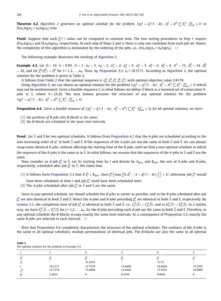
288 Y. Yin et al. / Information Sciences 189 (2012) 282–292
Theorem 4.2. Algorithm 2 generates an optimal schedule for the problem 1jpXj ¼ aX
j ð1� ktÞ; dAj ¼ dAj
PEA
j : f Bmax 6 U in
O(nA lognA + nB lognB) time.
Proof. Suppose that each f Xh ð�Þ value can be computed in constant time. The two sorting procedures in Step 1 require
O(nA lognA) and O(nB lognB), respectively. At each step of Steps 2 and 3, there is only one candidate from each job set. Hence,the complexity of this algorithm is dominated by the ordering of the jobs, i.e., O(nA lognA + nB lognB). h
The following example illustrates the working of Algorithm 2.
Example 4.3. Let D ¼ 16; k ¼ 0:05; U ¼ 1; nA ¼ 3; nB ¼ 2; aA1 ¼ 2; aA
2 ¼ 5; aA3 ¼ 3; aB
1 ¼ 2; aB2 ¼ 4; dA ¼ 15; dB
1 ¼ 14; dB2
¼ 16, and let f Bl ðE
Bl Þ ¼ EB
l for l = 1,2, . . . ,nB. Then, by Proposition 3.2, t0 = 10.3171. According to Algorithm 2, the optimalsolution for the problem is given in Table 2.
It follows from Table 2 that the optimal sequence is ðJ A2 ; J
B1 ; J
A3 ; J
B2 ; J
A1 Þ with optimal objective value 2.8178.
Using Algorithm 2, we can obtain an optimal solution for the problem 1jpXj ¼ aX
j ð1� ktÞ; dAj ¼ dAj
PEA
j : f Bmax 6 U which
may not be nondominated. Given a feasible sequence S, in what follows we define X-block as a maximal set of consecutive X-jobs in S, where X 2 {A,B}. The next lemma presents the structure of any optimal solution for the problem
1jpXj ¼ aX
j ð1� ktÞ; dAj ¼ dAj
PEA
j : f Bmax 6 U.
Proposition 4.4. Given a feasible instance of 1jpXj ¼ aX
j ð1� ktÞ; dAj ¼ dAj
PEA
j : f Bmax 6 U, for all optimal solutions, we have:
(1) the partition of B-jobs into B-blocks is the same;(2) the B-blocks are scheduled in the same time intervals.
Proof. Let eS and S be two optimal schedules. It follows from Proposition 4.1 that the A-jobs are scheduled according to the
non-increasing order of aAj in both eS and S. If the sequences of the A-jobs are not the same in both eS and S, we can always
swap some identical A-jobs, without affecting the starting time of the B-jobs, until we find a new optimal schedule in which
the sequence of the A-jobs is the same as in eS. In what follows, we assume that the sequences of the A-jobs in eS and S are thesame.
Now consider an A-job J Ah in eS. Let its starting time be t and denote by Aafter and Bafter the sets of A-jobs and B-jobs,
respectively, scheduled after job J Ah in eS. We claim that:
(1) It follows form Proposition 3.3 that if JBl 2 Bafter , then f B
l max 0; dBl � ðt þ aB
l ð1� ktÞÞn o� �
> U, otherwise job JBl would
have been scheduled at time t and job J Ah could have been scheduled later;
(2) The A-jobs scheduled after job J Ah in eS and S are the same.
Since in any optimal schedule, we should schedule the B-jobs as earlier as possible, and so the B-jobs scheduled after job
J Ah are also identical in both eS and S. Hence the A-jobs and B-jobs preceding J A
h are identical in both eS and S, respectively. By
Lemma 3.1, the completion time of job J Ah is identical in both eS and S, i.e., C A
h ðeSÞ ¼ C Ah ðSÞ, and so EA
h ðeSÞ ¼ EAh ðSÞ. In a similar
way, we have EAj ðeSÞ ¼ EA
j ðSÞ for j = 1,2, . . . ,nA. So, the B-jobs preceding each A-job are the same in both eS and S. Therefore, inany optimal schedule the B-blocks occupy exactly the same time intervals. As a consequence of Proposition 3.3, exactly thesame B-jobs are selected in each interval. h
Note that Proposition 4.4 completely characterizes the structure of the optimal schedules. The earliness of the A-jobs isthe same in all optimal schedules, modulo permutations of identical jobs. The B-blocks are also the same in all optimal
Table 2The optimal solution for the problem in Example 4.3.
r 1 2 3 4 5
JXj JA
2 JB1 JA
3 JB2 JA
1
sXj
– 12.2222 – 13.75 –
t 10.3171 12.7378 13.4640 14.4444 15.5555
CXj
12.7378 13.4640 14.4444 15.5555 16.0000
f Xj
2.2622 0 0.5556 0.4445 0

Y. Yin et al. / Information Sciences 189 (2012) 282–292 289
schedules, the only difference being the internal scheduling of each B-block. To find an optimal nondominated schedule, it issufficient to slightly modify the Algorithm 2. Denote EB
j ðtÞ by the earliness of job JBj if it is scheduled at time t
and let JBU be the unscheduled B-jobs. In Step 2 of Algorithm 2, we only need to schedule the job JB
l such that f Bl ðE
Bl ðtÞÞ ¼
minJBj 2JB
U ;fB
jðEB
j ðtÞÞ6Uff Bj ðE
Bj ðtÞÞg: Let S be the optimal schedule generated in this way.
Theorem 4.5. Consider a feasible instance of 1jpXj ¼ aX
j ð1� ktÞ; dAj ¼ dAj
PEA
j : f Bmax 6 U, the schedule S is nondominated.
Proof. Proposition 4.4 implies that the partition of B-jobs into B-blocks is the same for all optimal schedules. Since A-jobs do
not play any role within each block, the problem decomposes into several instances of 1jpXj ¼ aX
j ð1� ktÞ; dAj ¼ dAjf B
max, one
for each B-block. When building the schedule, if we pick every time the B-job with the minimum earliness cost, the very
same proof of Proposition 3.4 implies that S minimizes 1jpXj ¼ aX
j ð1� ktÞ; dAj ¼ dAjf B
max. h
Theorem 4.6. An optimal nondominated solution for the problem 1jpXj ¼ aX
j ð1� ktÞ; dAj ¼ dAj
PEA
j : f Bmax 6 U can be computed
in OðnA log nA þ n2BÞ time.
Proof. The proof is similar to that of Theorem 3.6. h
5. Problem 1jpXj ¼ aX
j ð1� ktÞ; dAj ¼ dAj+wA
j E Aj : f B
max <U
Mor and Mosheiov [24] showed that the problem 1jdAj ¼ dAj
PwA
j EAj : f B
max 6 U is binary NP-hard. Hence the problem
1jpXj ¼ aX
j ð1� ktÞ; dAj ¼ dAj
PwA
j EAj : f B
max 6 U must be binary NP-hard too. In the following we show that
1jpXj ¼ aX
j ð1� ktÞ; dAj ¼ dAj
PwA
j EAj : f B
max 6 U may be polynomially solvable if A-jobs have reversely agreeable weights,
i.e., aAj 6 aA
l implies wAj P wA
l for all A-jobs J Aj and J A
l . Note first that Propositions 3.2, 3.3, 3.4 still hold for this problem.
Now we provide Proposition 5.1 as follows.
Proposition 5.1. Consider a feasible instance of 1jpXj ¼ aX
j ð1� ktÞ; dAj ¼ dAj
PwA
j EAj : f B
max 6 U, if A-jobs have reverselyagreeable weights, then there is an optimal schedule in which the A-jobs are scheduled in a non-increasing order of aA
j =wAj .
Proof. Consider an optimal schedule S where the A-jobs are not ordered according to the non-increasing order of aAj =wA
j . Let
J Al and J A
h be the first pair of jobs such that aAl =wA
l < aAh =wA
h . Then aAl 6 aA
h and wAl P wA
h since A-jobs have reversely agreeable
weights. Assume that in schedule S, job J Al starts at time t, then a set of B-jobs are consecutively scheduled (with a total load
of, say, p), and then job J Ah . Furthermore, let p0 denote the set of jobs scheduled after job J A
h . We interchange jobs J Al and J A
h ,leaving the remaining jobs in their original positions, to derive a new schedule S0 from schedule S. Then by the proof
Proposition 4.1, we know that EAh ðS
0Þ 6 EAl ðSÞ; EA
l ðS0Þ ¼ EA
h ðSÞ and EAj ðS
0Þ ¼ EAj ðSÞ for all other job J A
k 2 J A=fJ Al ; J
Ah g, and that sche-
dule S0 is feasible. Now to show that schedule S0 is not a worse schedule than S, it suffices to show
wAh EA
h ðS0Þ þwA
l EAl ðS
0Þ 6 wAl EA
l ðSÞ þwAh EA
h ðSÞ:
Since EAh ðS
0Þ 6 E Al ðSÞ; EA
l ðS0Þ ¼ E A
h ðSÞ and EAh ðS
0ÞP EAl ðS
0Þ, we have
wAl EA
l ðSÞ þwAh E A
h ðSÞ � wAh EA
h ðS0Þ þwA
l E Al ðS
0Þ� �
P wAl E A
h ðS0Þ þwA
h E Al ðS
0Þ � wAh E A
h ðS0Þ þwA
l E Al ðS
0Þ� �
¼ ðwAl �wA
h Þ E Ah ðS
0Þ � EAl ðS
0Þ� �
P 0;
as required.Thus, repeating this interchange argument for all A-jobs not sequenced according to the non-increasing order of aA
j =wAj
will yield the proposition. h
Based on the results of Propositions 3.2, 3.3, 3.4 and 5.1, we can develop Algorithm 3 for the problem1jpX
j ¼ aXj ð1� ktÞ; dA
j ¼ dAjP
wAj EA
j : f Bmax 6 U in which A-jobs have reversely agreeable weights as follows.

290 Y. Yin et al. / Information Sciences 189 (2012) 282–292
Algorithm 3
Step 1:
Set t = t0, h = 1, and l = 1; sort the A-jobs in a non-increasing order of aAj =wAj , i.e.,
aA½1�=wA
½1� P aA½2�=wA
½2� P � � �P aA½nA �=wA
½nA �; calculate the critical starting time of each� �
B-job JBj from f Bj dB
j � ðsBj þ aB
j ð1� ksBj ÞÞ ¼ U, and sort them in a non-decreasing
order, i.e., sB½1� 6 sB
½2� 6 � � � 6 sB½nB �;
Step 2:
If l 6 nB, then If t P sB½l�, then
assign JB½l� at time t, set l ¼ lþ 1; t ¼ t þ aB
½l�ð1� ktÞ, and go to step 2;
Else go to step 3;
Else go to step 3;Step 3:
If h 6 nA, thenassign job J A½h� at time t, set h ¼ hþ 1; t ¼ t þ aA
½h�ð1� ktÞ, and go to step 2;
Else � �
Output the sequence S ¼ J½1�; J½2�; . . . ; J½nAþnB � .Theorem 5.2. If A-jobs have reversely agreeable weights, Algorithm 3 generates an optimal schedule for the problem1jpX
j ¼ aXj ð1� ktÞ; dA
j ¼ dAjP
wAj EA
j : f Bmax 6 U in O(nA lognA + nB lognB) time.
Proof. The proof is similar to that of Theorem 4.2. h
Now, we demonstrate the result of Algorithm 3 in the following example.
Example 5.3. Consider Example 4.3 and let wA1 ¼ 3; wA
2 ¼ 1 and wA3 ¼ 2. According to Algorithm 3, the optimal job sequence
is ðJ A2 ; J
B1 ; J
A3 ; J
B2 ; J
A1 Þ with optimal objective value 3.3734.
Using Algorithm 3, we can obtain an optimal solution for the problem 1jpXj ¼ aX
j ð1� ktÞ; dAj ¼ dAj
PwA
j EAj : f B
max 6 U such
that A-jobs have reversely agreeable weights, however this optimal schedule may not be nondominated. Note that Proposi-
tion 4.4 still holds for this problem. To find an optimal nondominated schedule, it is sufficient to slightly modify the algo-
rithm 3. Denote EBj ðtÞ by the earliness cost of job JB
j if it is scheduled at time t and let JBU be the unscheduled B-jobs. In
Step 2 of Algorithm 3, we only need to schedule the job JBl such that f B
l ðEBl ðtÞÞ ¼minJB
j 2JBU ;f
BjðEB
j ðtÞÞ6UfEBj ðtÞg. Let S be the optimal
schedule generated in this way.
Theorem 5.4. Consider a feasible instance of 1jpXj ¼ aX
j ð1� ktÞ; dAj ¼ dAj
PwA
j EAj : f B
max 6 U, if A-jobs have reversely agreeableweights, then the schedule S is nondominated.
Proof. The proof is similar to that of Theorem 4.5. h
Theorem 5.5. An optimal nondominated solution to the problem 1jpXj ¼ aX
j ð1� ktÞ; dAj ¼ dAj
PwA
j EAj : f B
max 6 U such that A-jobs
have reversely agreeable weights can be computed in OðnA log nA þ n2BÞ time.
Proof. The proof is similar to that of Theorem 3.6. h
6. Conclusions
In this paper, we introduced a new scheduling model with two-agent and a linear non-increasing deterioration simulta-neously. We focused our attention on the problem of finding an optimal schedule for agent A subject to the constraint thatthe maximum earliness cost for agent B does not exceed a given value. We proposed the optimal (nondominated) propertiesand the polynomial time algorithms for problems 1jpX
j ¼ aXj ð1� ktÞjf A
max : f Bmax 6 U and 1jpX
j ¼ aXj ð1� ktÞ; dA
j ¼ dAjP
EAj : f B
max
6 U, respectively. We also proved that the problems 1jpXj ¼ aX
j ð1� ktÞ; dAj ¼ dAj
PwjE
Aj : f B
max 6 U are polynomially solvable
Y. Yin et al. / Information Sciences 189 (2012) 282–292 291
under certain agreeable conditions. Another interesting future research direction is to analyze the scheduling problem withmore than two agents.
Acknowledgements
We are grateful to the Editor and three referees for their constructive comments on an earlier version of our paper. Thispaper was supported in part by the Natural Science Foundation for Young Scholars of Jiangxi, China (2010GQS0003); in partby the Science Foundation of Education Committee for Young Scholars of Jiangxi, China (GJJ11143); in part by the NSC underGrant No. NSC 99-2221-E-035-057-MY3.
References
[1] A. Agnetis, P.B. Mirchandani, D. Pacciarelli, A. Pacifici, Scheduling problems with two competing agents, Operations Research 52 (2004) 229–242.[2] A. Agnetis, D. Pacciarelli, A. Pacifici, Multi-agent single machine scheduling, Annals of Operations Research 150 (2007) 3–15.[3] B. Alidaee, N.K. Womer, Scheduling with time dependent processing times: review and extensions, Journal of the Operational Research Society 50
(1999) 711–729.[4] K.R. Baker, J.C. Smith, A multiple criterion model for machine scheduling, Journal of Scheduling 6 (2003) 7–16.[5] S. Balin, Parallel machine scheduling with fuzzy processing times using a robust genetic algorithm and simulation, Information Sciences 181 (17)
(2011) 3551–3569.[6] T.C.E. Cheng, Q. Ding, B.M.T. Lin, A concise survey of scheduling with time-dependent processing times, European Journal of Operational Research 152
(2004) 1–13.[7] T.C.E. Cheng, C.T. Ng, J.J. Yuan, Multi-agent scheduling on a single machine to minimize total weighted number of tardy jobs, Theoretical Computer
Science 362 (2006) 273–281.[8] T.C.E. Cheng, C.T. Ng, J.J. Yuan, Multi-agent scheduling on a single machine with max-form criteria, European Journal of Operational Research 188
(2008) 603–609.[9] T.C.E. Cheng, S.J. Yang, D.L. Yang, Common due-window assignment and scheduling of linear time-dependent deteriorating jobs and a deteriorating
maintenance activity, International Journal of Production Economics 135 (1) (2012) 154–161.[10] R.L. Graham, E.L. Lawler, J.K. Lenstra, A.H.G. Rinnooy Kan, Optimization and heuristic in deterministic sequencing and scheduling: a survey, Annals of
Discrete Mathematics 5 (1979) 287–326.[11] K.I.J. Ho, J.Y.T. Leung, W.-D. Wei, Complexity of scheduling tasks with time-dependent execution times, Information Processing Letter 48 (1993) 315–
320.[12] C.J. Hsu, T.C.E. Cheng, D.L. Yang, Unrelated parallel-machine scheduling with rate-modifying activities to minimize the total completion time,
Information Sciences 181 (20) (2011) 4799–4803.[13] K. Inderfurth, A. Janiak, M.Y. Kovalyov, F. Werner, Batching work and rework processes with limited deterioration of reworkables, Computers and
Operations Research 33 (2006) 1595–1605.[14] A. Janiak, M.Y. Kovalyov, Scheduling deteriorating jobs, in: A. Janiak (Ed.), Scheduling in Computer and Manufacturing Systems, Warszawa, WKL, 2006,
pp. 12–25.[15] W.H. Kuo, D.L. Yang, Note on ‘‘Single-machine and flowshop scheduling with a general learning effect model’’ and ‘‘Some single-machine and m-
machine flowshop scheduling problems with learning considerations, Information Sciences 180 (19) (2010) 3814–3816.[16] K. Lee, B.C. Choi, J.Y.T. Leung, M.L. Pinedo, Approximation algorithms for multi-agent scheduling to minimize total weighted completion time,
Information Processing Letters 109 (2009) 913–917.[17] W.C. Lee, S.K. Chen, W.C. Chen, C.C. Wu, A two-machine flowshop problem with two agents, Computers and Operations Research 38 (2011) 98–104.[18] W.C. Lee, S.K. Chen, C.C. Wu, Branch-and-bound and simulated annealing algorithms for a two-agent scheduling problem, Expert Systems with
Applications 37 (2010) 6594–6601.[19] W.C. Lee, P.J. Lai, Scheduling problems with general effects of deterioration and learning, Information Sciences 181 (6) (2011) 1164–1170.[20] Y. Li, G. Li, L. Sun, Z. Xu, Single machine scheduling of deteriorating jobs to minimize total absolute differences in completion Times, International
Journal of Production Economics 118 (2009) 424–429.[21] P. Liu, L.X. Tang, X.Y. Zhou, Two-agent group scheduling with deteriorating jobs on a single machine, The International Journal of Advanced
Manufacturing Technology 47 (2010) 657–664.[22] P. Liu, N. Yi, X.Y. Zhou, Two-agent single-machine scheduling problems under increasing linear deterioration, Applied Mathematical Modelling 35
(2011) 2290–2296.[23] M.M. Mazdeh, F. Zaerpour, A. Zareei, A. Hajinezhad, Parallel machines scheduling to minimize job tardiness and machine deteriorating cost with
deteriorating jobs, Applied Mathematical Modelling 34 (2010) 1498–1510.[24] B. Mor, G. Mosheiov, Scheduling problems with two competing agents to minimize minmax and minsum earliness measures, European Journal of
Operational Research 206 (2010) 540–546.[25] C.T. Ng, T.C.E. Cheng, A. Bachman, A. Janiak, Three scheduling problems with deteriorating jobs to minimize the total completion time, Information
Processing Letters 81 (2002) 327–333.[26] C.T. Ng, C.T.E. Cheng, J.J. Yuan, A note on the complexity of the two-agent scheduling on a single machine, Journal of Combinatorial optimization 12
(2006) 387–394.[27] Q.K. Pan, M. Fatih Tasgetiren, P.N. Suganthan, T.J. Chua, A discrete artificial bee colony algorithm for the lot-streaming flow shop scheduling problem,
Information Sciences 181 (12) (2011) 2455–2468.[28] X. Qi, F.S. Tu, Scheduling a single-machine to minimize earliness penalties subject to the SLK due-date determination method, European Journal of
Operational Research 105 (1998) 502–508.[29] D. Shabtay, Scheduling and due date assignment to minimize earliness, tardiness, holding, due date assignment and batch delivery costs, International
Journal of Production Economics 123 (2010) 235–242.[30] J.M.S. Valente, Local and global dominance conditions for the weighted earliness scheduling problem with no idle time, Computers & Industrial
Engineering 51 (2006) 765–780.[31] G. Wan, R.S. Vakati, J.Y.T. Leung, M. Pinedo, Scheduling two agents with controllable processing times, European Journal of Operational Research 205
(2010) 528–539.[32] J.B. Wang, A note on single-machine scheduling with decreasing time-dependent job processing times, Applied Mathematical Modelling 34 (2010)
294–300.[33] J.B. Wang, T.C.E. Cheng, Scheduling problems with the effects of deterioration and learning, Asia Pacific Journal of Operational Research 24 (2007) 245–
261.[34] J.B. Wang, Y. Jiang, G. Wang, Single-machine scheduling with past-sequence-dependent setup times and effects of deterioration and learning, The
International Journal of Advanced Manufacturing Technology 41 (2009) 1221–1226.
292 Y. Yin et al. / Information Sciences 189 (2012) 282–292
[35] X.R. Wang, X. Huang, J.B. Wang, Single-machine scheduling with linear decreasing deterioration to minimize earliness penalties, Applied MathematicalModelling 35 (2011) 3509–3515.
[36] L.Y. Wang, J.B. Wang, W.J. Gao, X. Huang, E.M. Feng, Two single-machine scheduling problems with the effects of deterioration and learning, TheInternational Journal of Advanced Manufacturing Technology 46 (2010) 715–720.
[37] X.Y. Wang, M.Z. Wang, J.B. Wang, Flow shop scheduling to minimize makespan with decreasing linear deterioration, Computers & IndustrialEngineering 60 (2011) 840–844.
[38] J.B. Wang, C.M. Wei, Parallel machines scheduling with a deteriorating maintenance activity and total absolute differences penalties, AppliedMathematics and Computation 217 (2011) 8093–8099.
[39] J.B. Wang, Z.Q. Xia, Scheduling jobs under decreasing linear deterioration, Information Processing Letter 94 (2005) 63–69.[40] C.C. Wu, W.C. Lee, Y.R. Shiau, Minimizing the total weighted completion time on a single machine under linear deterioration, International Journal of
Advanced Manufacturing Technology 33 (2007) 1237–1243.[41] Y. Yin, D. Xu, X. Huang, Notes on ‘‘some single-machine scheduling problems with general position-dependent and time-dependent learning effect,
Information Sciences 181 (11) (2011) 2209–2217.[42] S.J. Yang, D.L. Yang, Minimizing the makespan on single-machine scheduling with aging effect and variable maintenance activities, Omega 38 (2010)
528–533.[43] C. Zhao, H. Tang, A note to due-window assignment and single machine scheduling with deteriorating jobs and a rate-modifying activity, Computers
and Operations Research 39 (6) (2012) 1300–1303.[44] C. Zhao, H. Tang, Rescheduling problems with deteriorating jobs under disruptions, Applied Mathematical Modelling 34 (2010) 238–243.[45] C.L. Zhao, Q.L. Zhang, H.Y. Tang, Scheduling problems under linear deterioration, Acta Automatica Sinica 29 (2003) 531–535.