Scheduling Shop Scheduling - uni-bonn.de · basic scheduling decision for shop problems (see disj. ... Flow Shop models Makespan Minimization Lemma: For problem FjjCmax an optimal

SchedulingShop Scheduling

Tim Nieberg

Shop models: General Introduction

Remark: Consider non preemptive problems with regular objectives

Notation Shop Problems:

m machines, n jobs 1, . . . , n

operationsO = (i , j)|j = 1, . . . , n; i ∈ M j ⊂ M := 1, . . . ,m withprocessing times pij

M j is the set of machines where job j has to be processed on

PREC specifies the precedence constraints on the operations







Flow shop: M j = M andPREC = (i , j) → (i + 1, j)|i = 1, . . . ,m − 1; j = 1, . . . , n







Flow shop: M j = M andPREC = (i , j) → (i + 1, j)|i = 1, . . . ,m − 1; j = 1, . . . , n

Open shop: M j = M and PREC = ∅

Job shop: PREC contain a chain (i1, j) → . . . ,→ (i|M j |, j) foreach j


Disjunctive Formulation of the constraints

Cij denotes completion time of operation (i , j)

PREC have to be respected:





Cij − pij ≥ Ckl for all (k , l) → (i , j) ∈ PREC

no two operations of the same job are processed at the sametime:







Cij − pij ≥ Ckj or Ckj − pkj ≥ Cij for all i , k ∈ M j ; i 6= k

no two operations are processed jointly on the same machine:






Cij − pij ≥ Ckj or Ckj − pkj ≥ Cij for all i , k ∈ M j ; i 6= k

no two operations are processed jointly on the same machine:

Cij − pij ≥ Cil or Cil − pil ≥ Cij for all (i , j), (i , l) ∈ O; j 6= l

Cij − pij ≥ 0

the ’or’ constraints are called disjunctive constraints

some of the disjunctive constraints are ’overruled’ by thePREC constraints


Disjunctive Formulation - makes pan objective

minCmax

s.t.

Cmax ≥ Cij (i , j) ∈ O

Cij − pij ≥ Ckl (k , l) → (i , j) ∈ PREC

Cij − pij ≥ Ckj or Ckj − pkj ≥ Cij i , k ∈ M j ; i 6= k

Cij − pij ≥ Cil or Cil − pil ≥ Cij (i , j), (i , l) ∈ O; j 6= l

Cij − pij ≥ 0 (i , j) ∈ O


Disjunctive Formulation - sum objective

min∑

wjLj

s.t.

Lj ≥ Cij − dj (i , j) ∈ O

Cij − pij ≥ Ckl (k , l) → (i , j) ∈ PREC

Cij − pij ≥ Ckj or Ckj − pkj ≥ Cij i , k ∈ M j ; i 6= k

Cij − pij ≥ Cil or Cil − pil ≥ Cij (i , j), (i , l) ∈ O; j 6= l

Cij − pij ≥ 0 (i , j) ∈ O

Remark:

also other constraints, like e.g. release dates, can beincorporated

the disjunctive constraints make the problem hard (lead to anILP formulation)


Disjunctive Graph Formulation

graph representation used to represent instances and solutionsof shop problems

can be applied for regular objectives only


Disjunctive Graph G = (V ,C ,D)

V set of vertices representing the operations O

a vertex is labeled by the corresponding processing time;

Additionally, a source node 0 and a sink node ∗ belong to V ;their weights are 0

C set of conjunctive arcs reflecting the precedence constraints:for each (k , l) → (i , j) ∈ PREC a directed arc belongs to C

additionally 0 → O and O → ∗ are added to C

D set of disjunctive arcs representing ’conflicting’ operations:between each pair of operations belonging to the same job orto be processed on the same machine, for which no orderfollows from PREC , an undirected arc belongs to D


Disjunctive Graph - Example Job Shop

Data: 3 jobs, 3 machines;

M1 M2 M3

3

2 (1, 2) → (3, 2)

(3, 1) → (2, 1) → (1, 1)

(2, 3) → (1, 3) → (3, 3)

p31 = 4, p21 = 2, p11 = 1

p12 = 3, p32 = 3

p23 = 2, p13 = 4, p33 = 1

Jobs: 1


Disjunctive Graph - Example Job Shop

3

2 (1, 2) → (3, 2)

(3, 1) → (2, 1) → (1, 1)

(2, 3) → (1, 3) → (3, 3)

p31 = 4, p21 = 2, p11 = 1

p12 = 3, p32 = 3

p23 = 2, p13 = 4, p33 = 1

Jobs: 1

Graph:

0 ∗

Conjunctive arcs3,1 2,1

1,2

1,1

3,2

2,3 1,3 3,3

Disjunctive arcs


Disjunctive Graph - Example Open Shop

Data: 3 jobs, 3 machines;

3

2

Jobs: 1 (1, 1), (2, 1), (3, 1)

(1, 2), (2, 2), (3, 2)

(1, 3), (2, 3), (3, 3)

p11 = 4, p21 = 2, p31 = 1

p12 = 3, p22 = 1, p32 = 3

p13 = 2, p23 = 4, p33 = 1


Disjunctive Graph - Example Open Shop

3

2

Jobs: 1 (1, 1), (2, 1), (3, 1)

(1, 2), (2, 2), (3, 2)

(1, 3), (2, 3), (3, 3)

p11 = 4, p21 = 2, p31 = 1

p12 = 3, p22 = 1, p32 = 3

p13 = 2, p23 = 4, p33 = 1

Graph:

0 ∗

Conjunctive arcs2,1

1,2

3,3

Disjunctive arcs

1,1 3,1

2,2

1,3 2,3

3,2


Disjunctive Graph - Selection

basic scheduling decision for shop problems (see disj.formulation):define an ordering for operations connected by a disjunctivearc

→ turn the undirected disjunctive arc into a directed arc

selection S : a set of directed disjunctive arcs(i.e. S ⊂ D together with a chosen direction for each a ∈ S)

disjunctive arcs which have been directed are called ’fixed’

a selection is a complete selection if

each disjunctive arc has been fixedthe graph G (S) = (V , C ∪ S) is acyclic


Selection - Remarks

a feasible schedule induces a complete selection

a complete selection leads to sequences in which operationshave to be processed on machines

a complete selection leads to sequences in which operations ofa job have to be processed

Does each complete selection leads to a feasible schedule?


Calculate a Schedule for a Complete Selection S

calculated longest paths from 0 to all other vertices in G (S)

Technical description:

length of a path i1, i2, . . . , ir = sum of the weights of thevertices i1, i2, . . . , ircalculate length lij of the longest path from 0 to (i , j) (usinge.g. Dijkstra)start operation (i , j) at time lij − pij (i.e. Cij = lij )the length of a longest path from 0 to ∗ (such paths are calledcritical paths) is equal to the makespan of the schedule

resulting schedule is the semiactive schedule which respects allprecedence given by C and S


Reformulation Shop Problemfind a complete selection for which the corresponding scheduleminimizes the given (regular) objective function

Flow Shop models

Makespan Minimization

Lemma: For problem F ||Cmax an optimal schedule exists with

the job sequence on the first two machines is the samethe job sequence on the last two machines is the same

(Proof as Exercise)

Consequence: For F2||Cmax and F3||Cmax an optimal solutionexists which is a permutation solution

For Fm||Cmax , m ≥ 4, instances exist where no optimalsolution exists which is a permutation solution(Exercise)

Flow Shop models

Problem F2||Cmax

solution can be described by a sequence π

problem was solved by Johnson in 1954

Johnson’s Algorithm:

1 L = set of jobs with p1j < p2j ;

2 R = set of remaining jobs;

3 sort L by SPT w.r.t. the processing times on first machine(p1j )

4 sort R by LPT w.r.t. the processing times on second machine(p2j )

5 sequence L before R (i.e. π = (L,R) where L and R aresorted)

Flow Shop models

Example solution problem F2||Cmax

n = 5; p =

(

4 3 3 1 88 3 4 4 7

)

Flow Shop models


n = 5; p =

(

4 3 3 1 88 3 4 4 7

)

L = 1, 3, 4; R = 2, 5

sorting leads to L = 4, 3, 1; R = 5, 2

Flow Shop models


n = 5; p =

(

4 3 3 1 88 3 4 4 7

)

L = 1, 3, 4; R = 2, 5

sorting leads to L = 4, 3, 1; R = 5, 2

π = (4, 3, 1, 5, 2)

M2

3 1 525134

4M1

5 10 15 20 25

2

Flow Shop models

Problem F2||Cmax

Lemma 1: If

minp1i , p2j < minp2i , p1j

then job i is sequenced before job j by Johnson’s algorithm.

Lemma 2: If job j is scheduled immediately after job i and

minp1j , p2i < minp2j , p1i

then swapping job i and j does not increase Cmax .

Theorem: Johnson’s algorithm solves problem F2||Cmax

optimal in O(n log(n)) time.

(Proofs on the board)

Flow Shop models

Problem F3||Cmax

F3||Cmax is NP-hard in the strong sense

Reduction using 3-PARTITION

Proof on the board

Open Shop models

Algorithm Problem O2||Cmax

1 I = set of jobs with p1j ≤ p2j ; J = set of remaining jobs;2 IF p1r = maxmaxj∈I p1j ,maxj∈J p2j then

order on M1: (I \ r, J , r); order on M2: (r , I \ r, J)r first on M2, than on M1; all other jobs vice versa

M2

M1

r

rI \ r J

JI \ r

Open Shop models

Algorithm Problem O2||Cmax

1 I = set of jobs with p1j ≤ p2j ; J = set of remaining jobs;2 IF p1r = maxmaxj∈I p1j ,maxj∈J p2j then

order on M1: (I \ r, J , r); order on M2: (r , I \ r, J)r first on M2, than on M1; all other jobs vice versa

3 ELSE IF p2r = maxmaxj∈I p1j ,maxj∈J p2j then

order on M1: (r , J \ r, I ); order on M2: (J \ r, I , r)r first on M1, than on M2; all other jobs vice versa

M2

M1J \ r

J \ r

I

r

r

I

Open Shop models

Remarks Algorithm Problem O2||Cmax

complexity: O(n)

algorithm solves problem O2||Cmax optimally

Proof builds on fact that Cmax is either∑n

j=1 p1j or∑n

j=1 p2j orp1r + p2r

Open Shop models

Remarks Algorithm Problem O2||Cmax

complexity: O(n)

algorithm solves problem O2||Cmax optimally

Proof builds on fact that Cmax is either∑n

j=1 p1j or∑n

j=1 p2j orp1r + p2r

Problem O3||Cmax

Problem O3||Cmax is NP-hardProof as Exercise (Reduction using PARTITION)

Open Shop models

Problem O|pmtn|Cmax

define MLi :=∑n

j=1 pij (load of machine i)

define JLj :=∑m

i=1 pij (load of job j)

LB := maxmaxmi=1 MLi ,maxn

j=1 JLj is a lower bound onCmax

Open Shop models

Problem O|pmtn|Cmax

define MLi :=∑n

j=1 pij (load of machine i)

define JLj :=∑m

i=1 pij (load of job j)

LB := maxmaxmi=1 MLi ,maxn

j=1 JLj is a lower bound onCmax

Theorem: For problem O|pmtn|Cmax a schedule withCmax = LB exists.

Proof of the theorem is constructive and leads to a polynomialalgorithm for problem O|pmtn|Cmax

Open Shop models

Notations for Algorithm O|pmtn|Cmax

job j (machine i) is called tight if JLj = LB (MLi = LB)

job j (machine i) has slack if JLj < LB (MLi < LB)

a set D of operataions is called a decrementing set if it containfor each tight job and machine exactly one operation and foreach job and machine with slack at most one operation

Theorem: A decrementing set always exists and can becalculated in polynomial time(Proof based on maximal cardinality matchings; see e.g. P.Brucker: Scheduling Algorithms)

Open Shop models

Algorithm O|pmtn|Cmax

REPEAT

1 Calculate a decrementing set D;2 Calculate maximum value ∆ with

∆ ≤ min(i ,j)∈D pij

∆ ≤ LB − MLi if machine i has slack and no operation in D

∆ ≤ LB − JLj if job j has slack and no operation in D;

3 schedule the operations in D for ∆ time units in parallel;

4 Update values p, LB , JL, and ML

UNTIL all operations have been completely scheduled.

Open Shop models

Correctness Algorithm O|pmtn|Cmax

after an iteration we have: LBnew = LBold − ∆

in each iteration a time slice of ∆ time units is scheduled

the algorithm terminates after at most nm + n + m iterationssince in each iteration either

an operation gets completely scheduled orone additional machine or job gets tight

Open Shop models

Example Algorithm O|pmtn|Cmax

p ML

2 4 3 2 11p 3 1 2 3 9

2 3 3 2 10

JL 7 8 8 7 LB = 11

Open Shop models


∆ = 3 p ML

2 4 3 2 11p 3 1 2 3 9

2 3 3 2 10

JL 7 8 8 7 LB = 11

Open Shop models


∆ = 3 p ML

2 4 3 2 11p 3 1 2 3 9

2 3 3 2 10

JL 7 8 8 7 LB = 11

M1

M2

M3

3

1

2

3

Open Shop models


∆ = 3 p ML

2 4 3 2 11p 3 1 2 3 9

2 3 3 2 10

JL 7 8 8 7 LB = 11

M1

M2

M3

3

1

2

3

p ML

2 4 0 2 8p 0 1 2 3 6

2 0 3 2 7

JL 4 5 5 7 LB = 8

Open Shop models


∆ = 3 p ML

2 4 3 2 11p 3 1 2 3 9

2 3 3 2 10

JL 7 8 8 7 LB = 11

M1

M2

M3

3

1

2

3

∆ = 1 p ML

2 4 0 2 8p 0 1 2 3 6

2 0 3 2 7

JL 4 5 5 7 LB = 8

M1

M2

M3

3

1

2

3 4

2

Open Shop models


∆ = 1 p ML

2 4 0 2 8p 0 1 2 3 6

2 0 3 2 7

JL 4 5 5 7 LB = 8

M1

M2

M3

3

1

2

3 4

2

∆ = 3 p ML

2 3 0 2 7p 0 1 2 3 6

2 0 3 2 7

JL 4 4 5 7 LB = 7

M1

M2

M3

3

1

2

3 4 7

2

43

2

Open Shop models


∆ = 3 p ML

2 3 0 2 7p 0 1 2 3 6

2 0 3 2 7

JL 4 4 5 7 LB = 7

M1

M2

M3

3

1

2

3 4 7

2

43

2

∆ = 2 p ML

2 0 0 2 4p 0 1 2 0 3

2 0 0 2 4

JL 4 1 2 4 LB = 4

M1

M2

M3

3

1

2

3 4 7

2

43

9

4

3

1

2

Open Shop models


∆ = 2 p ML

2 0 0 2 4p 0 1 2 0 3

2 0 0 2 4

JL 4 1 2 4 LB = 4

M1

M2

M3

3

1

2

3 4 7

2

43

9

4

3

1

2

∆ = 1 p ML

2 0 0 0 2p 0 1 0 0 1

0 0 0 2 2

JL 2 1 0 2 LB = 2

M1

M2

M3

3

1

2

3 4 7

2

43

9

4

3

1

10

1

4

2

Open Shop models


∆ = 1 p ML

2 0 0 0 2p 0 1 0 0 1

0 0 0 2 2

JL 2 1 0 2 LB = 2

M1

M2

M3

3

1

2

3 4 7

2

43

9

4

3

1

10

1

4

2

∆ = 1 p ML

1 0 0 0 1p 0 1 0 0 1

0 0 0 1 1

JL 1 1 0 1 LB = 1

M1

M2

M3

3

1

2

3 4 7

2

43

9

4

3

1

10

1

4 4

2

11

12

Open Shop models

Final Schedule Example Algorithm O|pmtn|Cmax

p ML

2 4 3 2 11p 3 1 2 3 9

2 3 3 2 10

JL 7 8 8 7 LB = 11

M1

M2

M3

3

1

2

3 4 7

2

43

9

4

3

1

10

1

4 4

2

11

12

6 iterations

Cmax = 11 = LB

sequence of time slices may be changed arbitrary

Job Shop models

Problem J2||Cmax

I1: set of jobs only processed on M1

I2: set of jobs only processed on M2

I12: set of jobs processed first on M1 and than on M2

I21: set of jobs processed first on M2 and than on M1

π12: optimal flow shop sequence for jobs from I12

π21: optimal flow shop sequence for jobs from I21

Job Shop models

Algorithm Problem J2||Cmax

1 on M1 first schedule the jobs from I12 in order π12, than thejobs from I1, and last the jobs from I21 in order π21


M1

M2

I12 I1 I21

I2 I12I21

Job Shop models

Algorithm Problem J2||Cmax



M1

M2

I12 I1 I21

I2 I12I21

Theorem: The above algorithm solves problem J2||Cmax optimallyin O(n log(n)) time.Proof: almost straightforward!

Job Shop models

Problem J||Cmax

as a generalization of F ||Cmax , this problem is NP-hard

it is one of the most treated scheduling problems in literature

we presented

a branch and bound approacha heuristic approach called the Shifing Bottleneck Heuristic

for problem J||Cmax which both depend on the disjunctivegraph formulation

Job Shop models

Base of Branch and Bound

The set of all active schedules contains an optimal schedule

Solution method: Generate all active schedules and take thebest

Improvement: Use the generation scheme in a branch andbound setting

Consequence: We need a generation scheme to produce allactive schedules for a job shop

→ Approach: extend partial schedules

Job Shop models

Generation of all active schedules

Notations: (assuming that already a partial schedule S isgiven)

Ω: set of all operations which predecessors have already beenscheduled in S

rij :earliest possible starting time of operation (i , j) ∈ Ω w.r.t. S

Ω′: subset of Ω

Remark: rij can be calculated via longest path calculations inthe disjunctive graph belonging to S

Job Shop models

Generation of all active schedules (cont.)

1 (Initial Conditions)Ω := first operations of each job; rij := 0 for all (i , j) ∈ Ω;

2 (Machine selection)Compute for current partial schedulet(Ω) := min(i ,j)∈Ωrij + pij; i∗ := machine on whichminimum is achieved;

3 (Branching) Ω′ := (i∗, j)|ri∗j < t(Ω)FOR ALL (i∗, j) ∈ Ω′ DO

1 extend partial schedule by scheduling (i ∗, j) next on machinei∗;

2 delete (i∗, j) from Ω;3 add job-successor of (i∗, j) to Ω;4 Return to Step 2

Job Shop models

Generation of all active schedules - example

3

2 (1, 2) → (3, 2)

(3, 1) → (2, 1) → (1, 1)

(2, 3) → (1, 3) → (3, 3)

p31 = 4, p21 = 2, p11 = 1

p12 = 3, p32 = 3

p23 = 2, p13 = 4, p33 = 1

Jobs: 1

Partial Schedule:

M3

M2

M1

4 6

Job Shop models

Generation of all active schedules - example

3

2 (1, 2) → (3, 2)

(3, 1) → (2, 1) → (1, 1)

(2, 3) → (1, 3) → (3, 3)

p31 = 4, p21 = 2, p11 = 1

p12 = 3, p32 = 3

p23 = 2, p13 = 4, p33 = 1

Jobs: 1

Partial Schedule:

M3

M2

M1

4 6

Ω=(1, 1), (3, 2), (1, 3);r11 = 6, r32 = 4, r13 = 3;t(Ω) = min6 + 1, 4 + 3, 3 + 4 = 7;i∗ = M1;Ω′ = (1, 1), (1, 3)

Job Shop models

Generation of all active schedules - example (cont.)Partial Schedule:

M3

M2

M1

4 6

Ω=(1, 1), (3, 2), (1, 3);r11 = 6, r32 = 4, r13 = 3;t(Ω) = min6 + 1, 4 + 3, 3 + 4 = 7;i∗ = M1;Ω′ = (1, 1), (1, 3)Extended partial schedules:

M1

M2

M3

6 6

M1

M2

M3

Job Shop models

Remarks on the generation:

the given algorithm is the base of the branching

nodes of the branching tree correspond to partial schedules

Step 3 branches from the node corresponding to the currentpartial schedule

the number of branches is given by the cardinality of Ω′

a branch corresponds to the choice of an operation (i ∗, j) tobe schedules next on machine i ∗

→ a branch fixes new disjunctions

Job Shop models

Disjunctions fixed by a branching

Node v’

Node v with Ω′ = (i∗, j), (i∗, l)

Node v”

selection (i∗, j) selection (i∗, l)

Add disjunctions (i ∗, j) → (i∗k) for all unscheduled operations (i ∗, k) Add disjunctions (i ∗, l) → (i∗k) for all unscheduled operations (i ∗, k)

Consequence: Each node in the branch and bound tree ischaracterized by a set S ′ of fixed disjunctions

Job Shop models

Lower bounds for nodes of the branch and bound tree

Consider node V with fixed disjunctions S ′:

Simple lower bound:

calculate critical path in G (S ′)→ Lower bound LB(V )

Job Shop models

Lower bounds for nodes of the branch and bound tree

Consider node V with fixed disjunctions S ′:

Simple lower bound:

calculate critical path in G (S ′)→ Lower bound LB(V )

Better lower bound:

consider machine i

allow parallel processing on all machines 6= i

solve problem on machine i

Job Shop models

1-machine problem resulting for better LB

1 calculate earliest starting times rij of all operations (i , j) onmachine i (longest paths from source in G (S ′))

2 calculate minimum amount qij of time between end of (i , j)and end of schedule (longest path to sink in G (S ′))

3 solve single machine problem on machine i :

respect release datesno preemptionminimize maximum value of Cij + qij

Result: head-body-tail problem (see Lecture 3)

Job Shop models

Better lower bound

solve 1-machine problem for all machines

this results in values f1, . . . , fm

LBnew (V ) = maxmi=1 fi

Job Shop models

Better lower bound

solve 1-machine problem for all machines

this results in values f1, . . . , fm

LBnew (V ) = maxmi=1 fi

Remarks:

1-machine problem is NP-hard

computational experiments have shown that it pays of to solvethese m NP-hard problems per node of the search tree

20 × 20 job-shop instances are already hard to solve by branchand bound

Job Shop models

Better lower bound - examplePartial Schedule:

M1

M2

M3

3 6

Corresponding graph G (S ′):

3,1 2,1 1,1

1,2 3,20 *

2,3 1,3 3,3

Conjunctive arcs fixed disj.

Job Shop models

Graph G (S ′) with processing times:

3,1 2,1 1,1

1,2 3,2

2,3 1,3 3,3

4 2 1

3

3

2 4 1

0 *

LB(V )=l(0, (1, 2), (1, 3), (3, 3), ∗)=8

Job Shop models

Graph G (S ′) with processing times:

3,1 2,1 1,1

1,2 3,2

2,3 1,3 3,3

4 2 1

3

3

2 4 1

0 *

LB(V )=l(0, (1, 2), (1, 3), (3, 3), ∗)=8

Data for jobs on Machine 1:

green blue red

r12 = 0 r13 = 3 r11 = 6q12 = 5 q13 = 1 q11 = 0

Opt. solution: Opt = 8, LBnew (V ) = 8

M1

3 7 8

Job Shop models

Change p11 from 1 to 2!

3,1 2,1 1,1

1,2 3,2

2,3 1,3 3,3

4 2 2

3

3

2 4 1

0 *

LB(V ) = l(0, (1, 2), (1, 3), (3, 3), ∗) = l(0, (3, 1), (2, 1), (1, 1), ∗) = 8

Job Shop models

Change p11 from 1 to 2!

3,1 2,1 1,1

1,2 3,2

2,3 1,3 3,3

4 2 2

3

3

2 4 1

0 *

LB(V ) = l(0, (1, 2), (1, 3), (3, 3), ∗) = l(0, (3, 1), (2, 1), (1, 1), ∗) = 8

Data for jobs on Machine 1:

green blue red

r12 = 0 r13 = 3 r11 = 6q12 = 5 q13 = 1 q11 = 0

Opt. solution: OPT = 9, LBnew (V ) = 9

3 7 9M1

Job Shop models

The Shifting Bottleneck Heuristic

successful heuristic to solve makespan minimization for jobshop

iterative heuristic

determines in each iteration the schedule for one additionalmachine

uses reoptimization to change already scheduled machines

can be adapted to more general job shop problems

other objective functionsworkcenters instead of machinesset-up times on machines...

Shifting Bottleneck Heuristic for Job Shop

Basic Idea

Notation: M set of all machines

Given: fixed schedules for a subset M0 ⊂ M of machines (i.e.a selection of disjunctive arcs for cliques corresponding tothese machines)

Actions in one iteration:

select a machine k which has not been fixed (i.e. a machinefrom M \ M0)determine a schedule (selection) for machine k on the base ofthe fixed schedules for the machines in M0

reschedule the machines from M0 based on the other fixedschedules


Selection of a machine

Idea: Chose unscheduled machine which causes the mostproblems (bottleneck machine)

Realization:

Calculate for each operation on an unscheduled machine theearliest possible starting time and the minimal delay betweenthe end of the operation and the end of the complete schedulebased on the fixed schedules on the machines in M 0 and thejob orderscalculate for each unscheduled machine a schedule respectingthese earliest release times and delayschose a machine with maximal completion time and fix theschedule on this machine


Technical realization

Define graph G ′ = (N,A′):

N same node set as for the disjunctive graphA′ contains all conjunctive arcs and the disjunctive arcscorresponding to the selections on the machines in M 0

Cmax(M0) is the length of a critical path in G ′


Technical realization

Define graph G ′ = (N,A′):

N same node set as for the disjunctive graphA′ contains all conjunctive arcs and the disjunctive arcscorresponding to the selections on the machines in M 0

Cmax(M0) is the length of a critical path in G ′

Comments:

with respect to G ′ operations on machines from M \ M0 maybe processed in parallel

Cmax(M0) is the makespan of a corresponding schedule


Technical realization (cont.)

for an operation (i , j); i ∈ M \ M0 let

rij be the length of the longest path from 0 to (i , j) (withoutpij) in G ′

qij be the length of the longest path from (i , j) to ∗ (withoutpij) in G ′

Comments:

rij is the release time of (i , j) w.r.t. G ′

qij is the tail (minimal time till end) of (i , j) w.r.t. G ′


Technical realization (cont.)

For each machine from M \ M0 solve the nonpreemptiveone-machine head-body-tail problem 1|rj , dj < 0|Lmax

Result: values f (i) for all i ∈ M \ M0

Action:

Chose machine k as the machine with the largest f (i) valueschedule machine k according to the optimal schedule of theone-machine problemadd k to M0 and the corresponding disjunctive arcs to G ′

Cmax(M0 ∪ k) ≥ f (k)


Technical realization - Example

Given: M0 = M3 and on M3 sequence(3, 2) → (3, 1) → (3, 3)

Graph G ′:

3,1 2,1 1,1

1,2 3,2

2,3 1,3 3,3

4 2 1

33

24 1

0 *

Conjunctive arcs Selection M3

Cmax(M0) = 13


Technical realization - Example (cont.)

Machine M1:

(i , j) (1, 1) (1, 2) (1, 3)

rij 12 0 2

qij 0 10 1

pij 1 3 4



Machine M1:

(i , j) (1, 1) (1, 2) (1, 3)

rij 12 0 2

qij 0 10 1

pij 1 3 4

5 10 13

M1

101

1,2 1,3 1,1

f (M1) = 13



Machine M1:

(i , j) (1, 1) (1, 2) (1, 3)

rij 12 0 2

qij 0 10 1

pij 1 3 4

5 10 13

M1

101

1,2 1,3 1,1

f (M1) = 13

Machine M2:

(i , j) (2, 1) (2, 3)

rij 10 0

qij 1 5

pij 2 2



Machine M1:

(i , j) (1, 1) (1, 2) (1, 3)

rij 12 0 2

qij 0 10 1

pij 1 3 4

5 10 13

M1

101

1,2 1,3 1,1

f (M1) = 13

Machine M2:

(i , j) (2, 1) (2, 3)

rij 10 0

qij 1 5

pij 2 2

M2

5 10 13

5 1

2,12,3

f (M2) = 13



Choose machine M1 as the machine to fix the schedule:

add (1, 2) → (1, 3) → (1, 1) to G ′

M0 = M1, M3

3,1 2,1 1,1

1,2 3,2

2,3 1,3 3,3

4 2 1

33

24 1

0 *

Conjunctive arcs Selection M1, M3

Cmax(M0) = 13


Reschedule Machines

try to reduce the makespan of the schedule for the machinesin M0

Realization:

consider the machines from M0 one by oneremove the schedule of the chosen machine and calculate anew schedule based on the earliest starting times and delaysresulting from the other machines of M0 and the job orders


Technical realization reschedulingFor a chosen machine l ∈ M0 \ k do:

remove the arcs corresponding to the selection on machine l

from G ′

call new graph G ′′

calculate values rij , qij in graph G ′′

reschedule machine l according to the optimal schedule of thesingle machine head-body-tail problem


Technical realization rescheduling - Example

M0 \ k = M3, thus l = M3

removing arcs corresponding to M3 leads to graph G ′′:

3,1 2,1 1,1

1,2 3,2

2,3 1,3 3,3

4 2 1

33

24 1

0 *


Cmax(G′′) = 8;



M0 \ k = M3, thus l = M3


3,1 2,1 1,1

1,2 3,2

2,3 1,3 3,3

4 2 1

33

24 1

0 *


Cmax(G′′) = 8;

(i , j) (3, 1) (3, 2) (3, 3)

rij 0 3 7

qij 3 0 0

pij 4 3 1



M0 \ k = M3, thus l = M3


3,1 2,1 1,1

1,2 3,2

2,3 1,3 3,3

4 2 1

33

24 1

0 *


Cmax(G′′) = 8;

(i , j) (3, 1) (3, 2) (3, 3)

rij 0 3 7

qij 3 0 0

pij 4 3 1

33

M3

5 8

3,1 3,2 3,3

f (M3) = 8


Technical realization rescheduling - Example (cont.)

add (3, 1) → (3, 2) → (3, 3) to G ′′

New graph:

3,1 2,1 1,1

1,2 3,2

2,3 1,3 3,3

4 2 1

33

24 1

0 *


C newmax (M0) = 8


Heuristic: summary

1 Initialization:1 M0 := ∅;2 G := graph with all conjunctive arcs;3 Cmax (M

0) := length longest path in G :

2 Analyze unscheduled machines:

FOR ALL i ∈ M \ M0 DO

FOR ALL operation (i , j) DO

1 rij := length longest path from 0 to (i , j) in G ;

2 qij := length longest path from (i , j) to ∗ in G ;solve single machine head body tail problem → f (i)


Heuristic: summary (cont.)

3 Bottleneck selection:1 determine k such that f (k) = maxi∈M\M0 f (i);2 schedule machine k according to the optimal solution in Step

2;3 add corresponding disjunctive arcs to G ;4 M0 := M0 ∪ k;


Heuristic: summary (cont.)

4 Resequencing of machines:

FOR ALL i ∈ M0 \ k DO

1 delete disjunctive arcs corresponding to machine k from G ;

2 FOR ALL operation (i , j) DO

1 rij := length longest path from 0 to (i , j) in G ;

2 qij := length longest path from (i , j) to ∗ in G ;

3 solve single machine head body tail problem → f (i)

4 insert corresponding disjunctive arcs to G ;5 Stopping condition

IF M0 = M THEN Stop ELSE go to Step 2;


SBH - Example (cont.)M0 = M1,M3; thus M2 is bottleneck

graph G :

3,1 2,1 1,1

1,2 3,2

2,3 1,3 3,3

4 2 1

33

24 1

0 *


Cmax(G ) = 8;



graph G :

3,1 2,1 1,1

1,2 3,2

2,3 1,3 3,3

4 2 1

33

24 1

0 *


Cmax(G ) = 8;

(i , j) (2, 1) (2, 3)

rij 4 0

qij 1 5

pij 2 2



graph G :

3,1 2,1 1,1

1,2 3,2

2,3 1,3 3,3

4 2 1

33

24 1

0 *


Cmax(G ) = 8;

(i , j) (2, 1) (2, 3)

rij 4 0

qij 1 5

pij 2 2

2,3 2,1

1

5

M2

5 8

f (M2) = 7


SBH - Example (cont.)

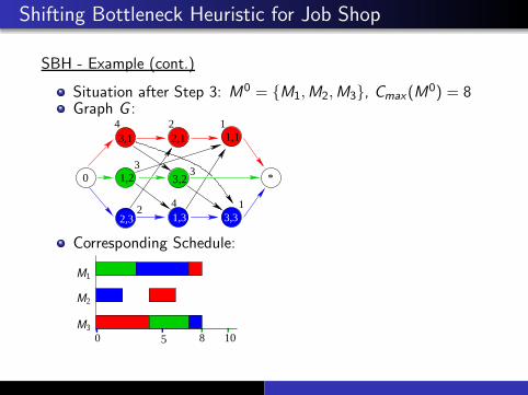
Situation after Step 3: M0 = M1,M2,M3, Cmax(M0) = 8

Graph G :

3,1 2,1 1,1

1,2 3,2

2,3 1,3 3,3

4 2 1

33

24 1

0 *


SBH - Example (cont.)

Situation after Step 3: M0 = M1,M2,M3, Cmax(M0) = 8

Graph G :

3,1 2,1 1,1

1,2 3,2

2,3 1,3 3,3

4 2 1

33

24 1

0 *

Corresponding Schedule:

5 1080

M1

M2

M3


An Important Subproblem

within the SBH the one-machine head-body-tail problemoccurs frequently:

this problem was also used within branch and bound tocalculate lower bounds

the problem is NP-hard (see Lecture 3)

there are efficient branch and bound methods for smallerinstances (see also Lecture 3)

the actual one-machine problem is a bit more complicatedthan stated in Lecture 3 (see following example)


Example Delayed Precedences

Jobs: (1, 1) → (2, 1)

(2, 2) → (1, 2)

(3, 3)

(3, 4)

Processing Times: p11 = 1, p21 = 1p22 = 1, p12 = 1p33 = 4p34 = 4

Initial graph G :

1,1 2,1

2,2 1,2

3,3

3,4

0 *


Example Delayed Precedences (cont.)

after 2 iterations SBH we get:M0 = M3,M1; (3, 4) → (3, 3) and (1, 2) → (1, 1)

Resulting graph G : (Cmax(M0) = 8)

1,1 2,1

2,2 1,2

3,3

3,4

1 1

1 1

4

4

0 *



3. iteration: only M2 unscheduled(i , j) pij rij qij

(2, 1) 1 3 0(2, 2) 1 0 3

Possible schedules for M2:

50 8M2

50 8M2



Both schedules are feasible and might be added to currentsolution

But: second schedule leads to

1,1 2,1

2,2 1,2

3,3

3,4

1 1

1 1

4

4

0 *

which contains a cycle


Delayed Precedences

The example shows:

not all solutions of the one-machine problem fit to the givenselections for machines from M0

the given selections for machines from M0 may induceprecedences for machines from M \ M0

Example:

scheduling operation (1, 2) before (1, 1) on M1 induces adelayed precedence constraint between (2, 2) and (2, 1) oflength 3→ operation (2, 1) has to start at least 3 time units after (2, 2)this time is needed to process operations (2, 2), (1, 2), and(1, 1)


Rescheduling Machines

after adding a new machine to M0, it may be worth to putmore effort in rescheduling the machines:

do the rescheduling in some specific order (e.g. based on their’head-body-tail’ values)repeat the rescheduling process until no improvement is foundafter rescheduling one machine, make a choice which machineto reschedule next (allowing that certain machines arerescheduled more often)...

practical test have shown that these extra effort often pays off

Documents

Scheduling Shop Scheduling - uni-bonn.de · basic scheduling decision for shop problems (see disj. ... Flow Shop models Makespan Minimization Lemma: For problem FjjCmax an optimal