ISSN 8755-6839

SCIENCE OF TSUNAMI HAZARDS

Journal of Tsunami Society International

Volume 35 Number 2 2016

TSUNAMI DISPERSION SENSITIVITY TO SEISMIC SOURCE PARAMETERS

Oleg Igorevich Gusev, Sofya Alexandrovna Beisel

Institute of Computational Technologies of SB RAS, 6 Acad. Lavrentjev Avenue, 630090

Novosibirsk, Russia

ABSTRACT

The study focuses on the sensitivity of frequency dispersion effects to the form of initial surface elevation of seismic tsunami source. We vary such parameters of the source as rupture depth, dip-angle and rake-angle. Some variations in magnitude and strike angle are considered. The fully nonlinear dispersive model on a rotating sphere is used for wave propagation simulations. The main feature of the algorithm is the splitting of initial system on two subproblems of elliptic and hyperbolic type, which allows implementation of well-suitable numerical methods for them. The dispersive effects are estimated through differences between computations with the dispersive and nondispersive models. We consider an idealized test with a constant depth, a model basin for near-field tsunami simulations and a realistic scenario. Our computations show that the dispersion effects are strongly sensitive to the rupture depth and the dip-angle variations. Waves generated by sources with lager magnitude may be even more affected by dispersion.

Keywords: seismic source, tsunami propagation, frequency dispersion, fully nonlinear dispersive model, rotating sphere, numerical modelling.

Vol. 35, No. 2, Page 84, (2016)

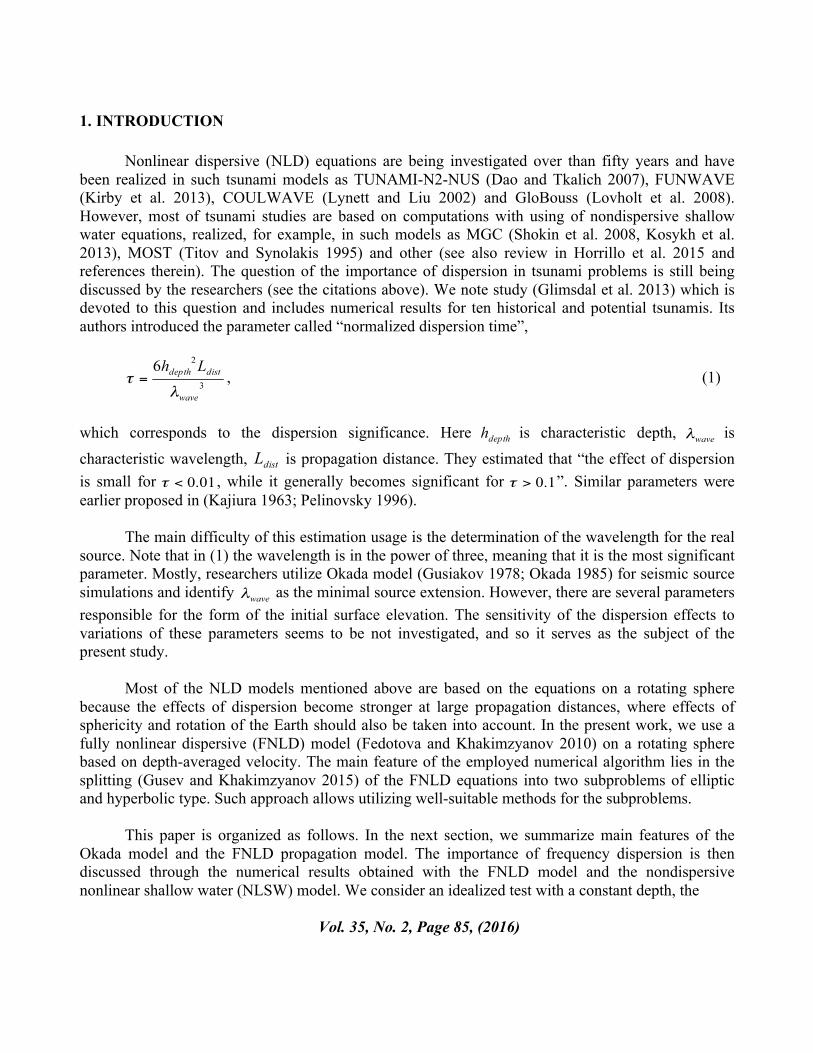
1. INTRODUCTION

Nonlinear dispersive (NLD) equations are being investigated over than fifty years and have been realized in such tsunami models as TUNAMI-N2-NUS (Dao and Tkalich 2007), FUNWAVE (Kirby et al. 2013), COULWAVE (Lynett and Liu 2002) and GloBouss (Lovholt et al. 2008). However, most of tsunami studies are based on computations with using of nondispersive shallow water equations, realized, for example, in such models as MGC (Shokin et al. 2008, Kosykh et al. 2013), MOST (Titov and Synolakis 1995) and other (see also review in Horrillo et al. 2015 and references therein). The question of the importance of dispersion in tsunami problems is still being discussed by the researchers (see the citations above). We note study (Glimsdal et al. 2013) which is devoted to this question and includes numerical results for ten historical and potential tsunamis. Its authors introduced the parameter called “normalized dispersion time”,

, (1)

which corresponds to the dispersion significance. Here is characteristic depth, is characteristic wavelength, is propagation distance. They estimated that “the effect of dispersion is small for , while it generally becomes significant for ”. Similar parameters were earlier proposed in (Kajiura 1963; Pelinovsky 1996).

The main difficulty of this estimation usage is the determination of the wavelength for the real source. Note that in (1) the wavelength is in the power of three, meaning that it is the most significant parameter. Mostly, researchers utilize Okada model (Gusiakov 1978; Okada 1985) for seismic source simulations and identify as the minimal source extension. However, there are several parameters responsible for the form of the initial surface elevation. The sensitivity of the dispersion effects to variations of these parameters seems to be not investigated, and so it serves as the subject of the present study.

Most of the NLD models mentioned above are based on the equations on a rotating sphere

because the effects of dispersion become stronger at large propagation distances, where effects of sphericity and rotation of the Earth should also be taken into account. In the present work, we use a fully nonlinear dispersive (FNLD) model (Fedotova and Khakimzyanov 2010) on a rotating sphere based on depth-averaged velocity. The main feature of the employed numerical algorithm lies in the splitting (Gusev and Khakimzyanov 2015) of the FNLD equations into two subproblems of elliptic and hyperbolic type. Such approach allows utilizing well-suitable methods for the subproblems.

This paper is organized as follows. In the next section, we summarize main features of the

Okada model and the FNLD propagation model. The importance of frequency dispersion is then discussed through the numerical results obtained with the FNLD model and the nondispersive nonlinear shallow water (NLSW) model. We consider an idealized test with a constant depth, the

Vol. 35, No. 2, Page 85, (2016)

model basin “Wash-tube” for near-field tsunami computations and a realistic scenario.

2. TSUNAMI MODEL DESCRIPTION

2.1. Seismic source model

In our computations, seismic tsunami sources are generated according to the standard method (Okada 1985), in which the seafloor deformation is computed in a homogeneous elastic half-space with a planar dislocation and then specified on the free surface as an initial condition, with zero initial flow velocity. Such internal dislocation source is characterized by the following parameters: the source centroid location, the width and the length of the fault, and , respectively, the depth of the upper bound of the fault, , the fault slip value, , the angle between the fault and a horizontal plane (dip-angle), , the fault direction relative to north (strike-angle), , and the slip direction (rake-angle), . We use program complex MGC for computation of initial surface disturbance of seismic source.

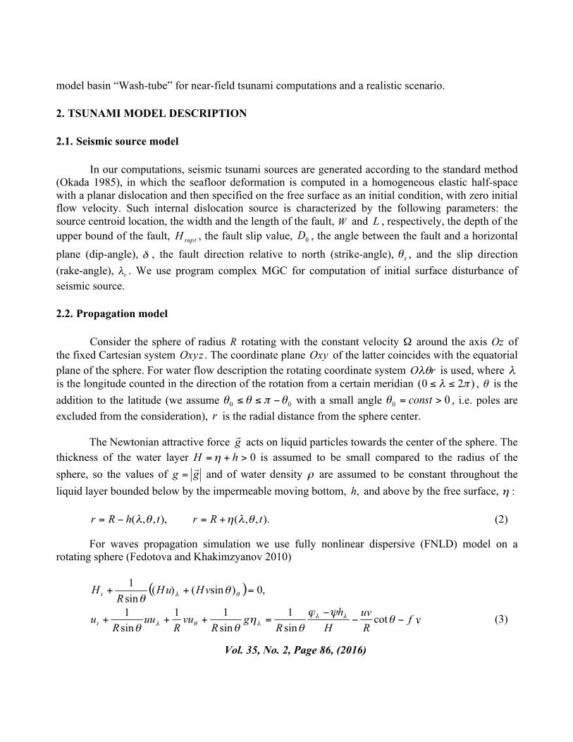
2.2. Propagation model

Consider the sphere of radius rotating with the constant velocity around the axis of the fixed Cartesian system . The coordinate plane of the latter coincides with the equatorial plane of the sphere. For water flow description the rotating coordinate system is used, where is the longitude counted in the direction of the rotation from a certain meridian , is the addition to the latitude (we assume with a small angle , i.e. poles are excluded from the consideration), is the radial distance from the sphere center.

The Newtonian attractive force acts on liquid particles towards the center of the sphere. The thickness of the water layer is assumed to be small compared to the radius of the sphere, so the values of and of water density are assumed to be constant throughout the liquid layer bounded below by the impermeable moving bottom, and above by the free surface,

(2)

For waves propagation simulation we use fully nonlinear dispersive (FNLD) model on a rotating sphere (Fedotova and Khakimzyanov 2010)

      (3)

Vol. 35, No. 2, Page 86, (2016)

Here the symbols and denote the physical components of the velocity vector

( , , , ), and is the Coriolis parameter, expressed

in terms of latitude’s addition . The functions and included in the right sides of equations (3) are the dispersive

components of the depth-integrated pressure and the pressure at the bottom respectively, , .

Dispersive additives are expressed by the following formulas:

, ,

where , , ,

, ,

, , .

In detail

,

,

, .

FNLD model (3) is called “fully” because it is derived without the assumption on the

smallness of wave amplitudes, and all the nonlinear terms associated with dispersion are stored. So, one can use it for calculation of the surface wave propagation over an uneven bottom both in a deep water and in a coastal zone. The FNLD model allows also to simulate the wave generation by the long-time shifts of bottom fragments, which extends the range of problems that can be solved within the framework of the known NLD models on a sphere (Dao and Tkalich 2007; Lovholt at al. 2008; Kirby et al. 2013).

Vol. 35, No. 2, Page 87, (2016)

Moreover, FNLD model can be written in the quasi conservative form of mass and momentum

balances (Fedotova and Khakimzyanov 2014), and it has the balance equation of the total energy, agreed with the similar equation of the 3D-model, which not only confirms the physical consistency of the model, but also allows an additional control of the calculations.

System (3) is not a system of Cauchy–Kovalevskaya type because the equations of motion contain the mixed third-order derivatives of the velocity vector components with respect to time and space. A direct approximation of the derivatives leads to a complex problem, which is difficult to solve. In the case of a plane geometry, it turned out fruitful (Gusev 2014; Khakimzyanov et al. 2015) to split the original system on the scalar equation of elliptic type and the system of hyperbolic equations. In the present work, we use this approach to equations (3) on a rotating sphere.

The splitting of system (3) results in the hyperbolic equations

(4)

with first-order derivatives only, and the uniformly elliptic equation for the dispersive component

(5)

where

,

Vol. 35, No. 2, Page 88, (2016)

, .

Note that neither the left nor the right part of (5) does not contain time derivatives of the

dependent variables , and . Values of the dispersive component are calculated from the expression

.

Supposing , one obtain NLSW model (Cherevko and Chupakhin 2009) on a rotating sphere.

We note that the still water level doesn’t have a spherical form, and can be described by the equation , where

.

It is natural to measure the free surface and the depth not as deviations (2) from a sphere surface, but as the deviations and from the still water level. These functions are connected with (2) as

, . We construct a numerical algorithm for extended system (4), (5) as alternate solving of the

hyperbolic and the elliptic subproblems on each time step. Such approach allows us to use well-suitable methods for them. The hyperbolic system is implemented using a second-order predictor-corrector scheme, and the elliptic equation is solved by integro-interpolation and SOR methods. Totally, we develop the algorithm of second-order approximation in space and time. For a more detailed description of the model, see (Gusev and Khakimzyanov 2015). Some properties of the algorithm, such as correctness, stability, numerical dispersion and dissipation, were investigated in studies (Gusev 2012; Fedotova et al. 2015). Considering the sphericity and rotation effects are small in some tests presented below, we use also a plane analogue of the model (Gusev 2014; Khakimzyanov et al. 2015). In the next section, we estimate frequency dispersion influence comparing the numerical solutions obtained with the FNLD and the NLSW models.

Vol. 35, No. 2, Page 89, (2016)

RESULTS OF COMPUTATIONS

2.3. Flat bottom test

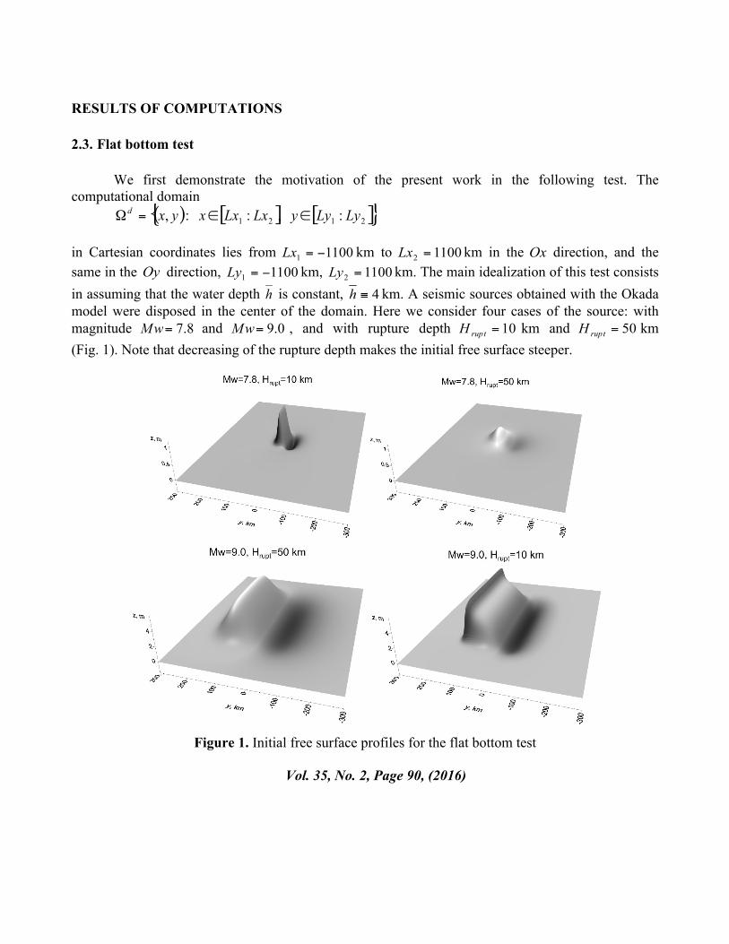
We first demonstrate the motivation of the present work in the following test. The computational domain

in Cartesian coordinates lies from km to km in the direction, and the same in the direction, km, km. The main idealization of this test consists in assuming that the water depth is constant, km. A seismic sources obtained with the Okada model were disposed in the center of the domain. Here we consider four cases of the source: with magnitude and , and with rupture depth km and km (Fig. 1). Note that decreasing of the rupture depth makes the initial free surface steeper.

Figure 1. Initial free surface profiles for the flat bottom test

Vol. 35, No. 2, Page 90, (2016)

For the computations, we utilize an uniform grid

.

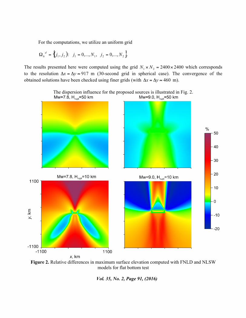
The results presented here were computed using the grid which corresponds to the resolution m (30-second grid in spherical case). The convergence of the obtained solutions have been checked using finer grids (with m).

The dispersion influence for the proposed sources is illustrated in Fig. 2.

Figure 2. Relative differences in maximum surface elevation computed with FNLD and NLSW models for flat bottom test

Vol. 35, No. 2, Page 91, (2016)

Here we show the relative differences ((NLSW-FNLD)/NLSW) in the maximum surface elevation computed with the FNLD and the NLSW models. As one would expect, the lowest dispersion effects are observed in the case with and km, and the highest are observed in the case with and km. Increase of the magnitude leads to the increase of the effective extent of the initial wave profile, and decrease of the rupture depth makes the profile steeper. Surprisingly, the simulations show that the waves in the case with and km are much less affected by dispersion than the ones with and km. It means that the determinative factor for the dispersion effects is not an effective extent of the initial disturbance, but its form.

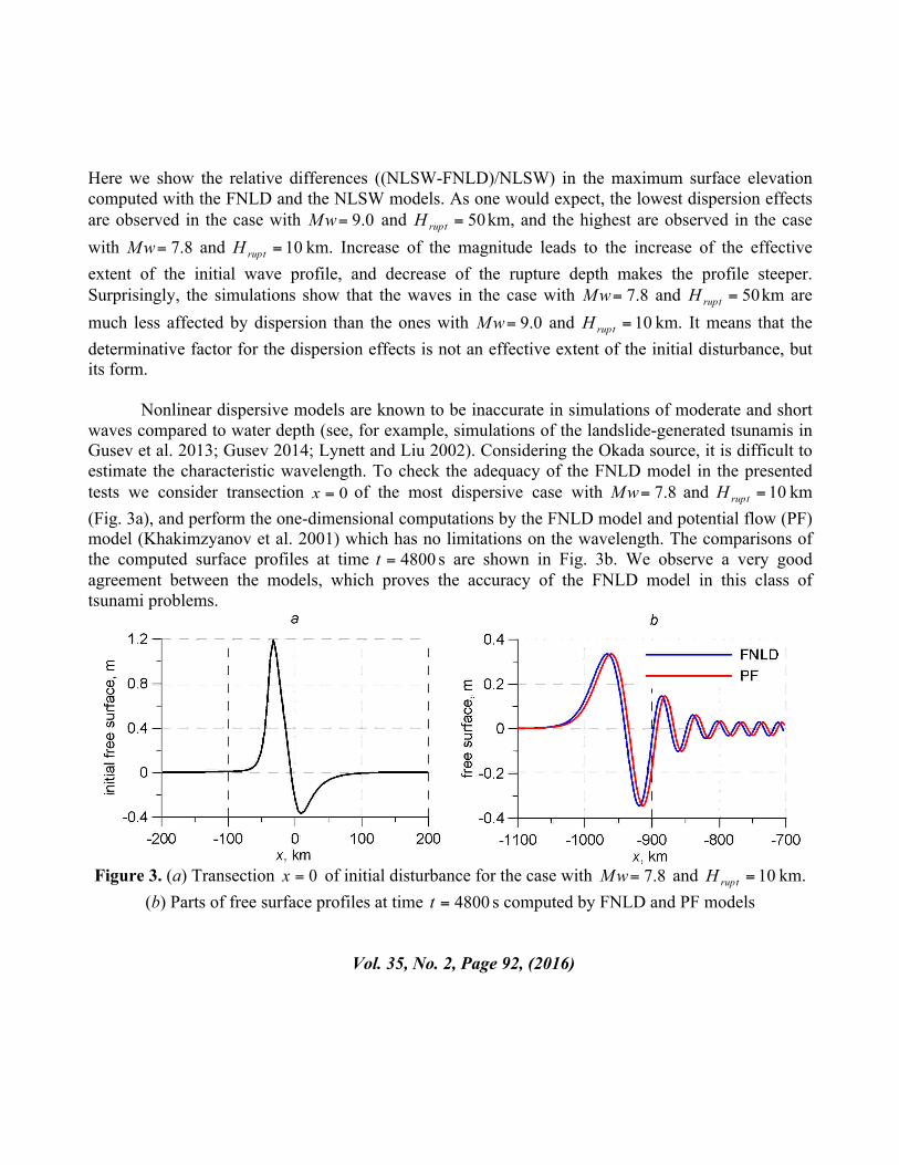
Nonlinear dispersive models are known to be inaccurate in simulations of moderate and short waves compared to water depth (see, for example, simulations of the landslide-generated tsunamis in Gusev et al. 2013; Gusev 2014; Lynett and Liu 2002). Considering the Okada source, it is difficult to estimate the characteristic wavelength. To check the adequacy of the FNLD model in the presented tests we consider transection of the most dispersive case with and km (Fig. 3a), and perform the one-dimensional computations by the FNLD model and potential flow (PF) model (Khakimzyanov et al. 2001) which has no limitations on the wavelength. The comparisons of the computed surface profiles at time s are shown in Fig. 3b. We observe a very good agreement between the models, which proves the accuracy of the FNLD model in this class of tsunami problems.

Figure 3. (a) Transection of initial disturbance for the case with and km.

(b) Parts of free surface profiles at time s computed by FNLD and PF models

Vol. 35, No. 2, Page 92, (2016)

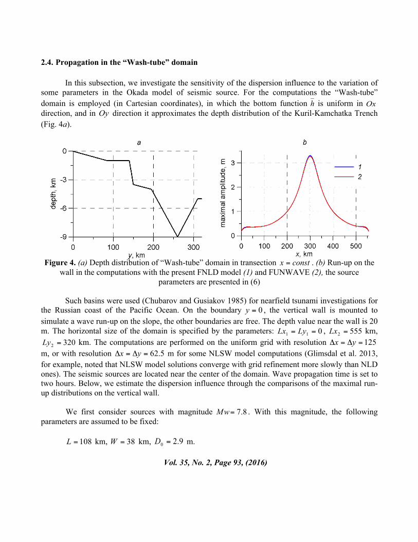
2.4. Propagation in the “Wash-tube” domain

In this subsection, we investigate the sensitivity of the dispersion influence to the variation of some parameters in the Okada model of seismic source. For the computations the “Wash-tube” domain is employed (in Cartesian coordinates), in which the bottom function is uniform in direction, and in direction it approximates the depth distribution of the Kuril-Kamchatka Trench (Fig. 4a).

Figure 4. (a) Depth distribution of “Wash-tube” domain in transection . (b) Run-up on the

wall in the computations with the present FNLD model (1) and FUNWAVE (2), the source parameters are presented in (6)

Such basins were used (Chubarov and Gusiakov 1985) for nearfield tsunami investigations for

the Russian coast of the Pacific Ocean. On the boundary , the vertical wall is mounted to simulate a wave run-up on the slope, the other boundaries are free. The depth value near the wall is 20 m. The horizontal size of the domain is specified by the parameters: , km,

km. The computations are performed on the uniform grid with resolution m, or with resolution m for some NLSW model computations (Glimsdal et al. 2013, for example, noted that NLSW model solutions converge with grid refinement more slowly than NLD ones). The seismic sources are located near the center of the domain. Wave propagation time is set to two hours. Below, we estimate the dispersion influence through the comparisons of the maximal run-up distributions on the vertical wall.

We first consider sources with magnitude . With this magnitude, the following parameters are assumed to be fixed:

km, km, m.

Vol. 35, No. 2, Page 93, (2016)

To verify our two-dimensional code in this class of problems we make the comparison of obtained numerical solution of the FNLD model with the one of fully nonlinear model FUNWAVE (https://www.udel.edu/kirby/programs/funwave/funwave.html, Shi et al. 2012). The source parameters have the values

, , , km. (6)

The results of the comparison of the computed run-ups on the wall are presented in Fig. 4b. The excellent agreement between the models is observed. Note that the FUNWAVE computations were performed on a grid with resolution m, that two times coarser than the grid in FNLD model computations. Nevertheless, the computation time (on a single CPU) and the size of the used memory were similar. For other verifications of the FNLD model in two-dimensional case, see (Gusev 2014).

2.4.1. Rupture depth variation

The first set of the computations is devoted to the variation of rupture depth from km to km with a step equal to km. The other parameters of the sources are put as follows:

, , .

The features of initial free surfaces and the obtained results are shown in Fig. 5. Here and below we illustrate the cross-sections km of the initial surface elevations on the upper graph, obtained run-ups on the lowest one and corresponding absolute (NLSW-FNLD) and relative ((NLSW-FNLD)/NLSW) differences in the middle part of the figure. In this case, Fig. 5 clearly shows that the decrease of significantly increases the maximal run-ups on the wall and the influence of dispersion. The reason is higher and steeper profile of the initial surface elevation. The absolute differences reach values up to m while the relative ones amount up to %. The relative differences may behave intricately near the bounds ( and km) where the run-ups are small, so we cut the corresponding graphs at some distance from these bounds. 2.4.2. Dip-angle variation

For the computations with variation of we consider two cases of the strike-angle: and The dip-angle is changed from to with a step equal

to .The rake angle is fixed, , while the rupture depth is varied from km to km for the conservation of the position of the lower bound of the fault.

Vol. 35, No. 2, Page 94, (2016)

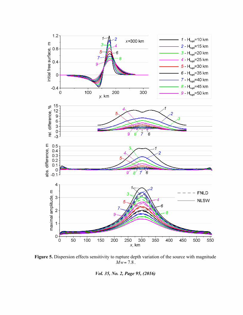
Figure 5. Dispersion effects sensitivity to rupture depth variation of the source with magnitude .

Vol. 35, No. 2, Page 95, (2016)

Fig. 6 illustrates the results of the computations with . It shows that the maximal run-ups is fixed with the minimal dip-angle, , despite the fact that initial free surface was not

Figure 6. Dispersion effects sensitivity to dip-angle variation of the source with magnitude .

Case with

Vol. 35, No. 2, Page 96, (2016)

the highest in this case. Such effect is associated with the depression wave arrived at the wall before the main positive one (see, for example, Tadepalli and Synolakis 1994; Didenkulova et al. 2014). Vice versa, with the depression wave arrived after the main positive one and the run-ups are minimal. The maximal dispersion effects are observed in the cases with and , when the initial free surfaces are the highest. The absolute differences are up to m while the relative ones are up to %.

Changing the strike-angle to rotates the initial free surfaces 180 degrees in the horizontal plane. The obtained results (Fig. 7) have some differences from the previous set of experiments. Again, the sources with the depression part located farther from the wall than the positive elevation ( ) generate lower run-ups which are less affected by dispersion. The increase of the dip-angle ( ) increases the run-ups, but the dispersion influence is not trivial in these cases. Fig. 7 shows that the differences in the NLSW and the FNLD computations become negative at approximately 50 km far from the abscissa of the run-up maximum, meaning that the dispersion effects increase the wave height there. Regard to the absolute differences, the maximal one ( m) is obtained with while the minimum one ( m) corresponds to Maximal relative differences ( ) are observed with , and , the minimal one ( ) is computed with . 2.4.3. Rake-angle variation

The rake-angle is changed from to with a step equal to . The other parameters are assigned as follows:

km, , .

Fig. 8 shows the results of the computations. At the upper panel of the figure, we bring the main fragments of the initial free surface elevations for clearer comparisons. The computations show that the variation of the rake-angle has a strong influence on the run-up, increasing it with the increase of

. The absolute differences in the NLSW and the FNLD behave similarly and reach m. However, the relative differences have the inverse behavior, tending to decrease it values with increase of . The maximal relative differences are observed far from the center of the wall where the run-ups are small.

Vol. 35, No. 2, Page 97, (2016)

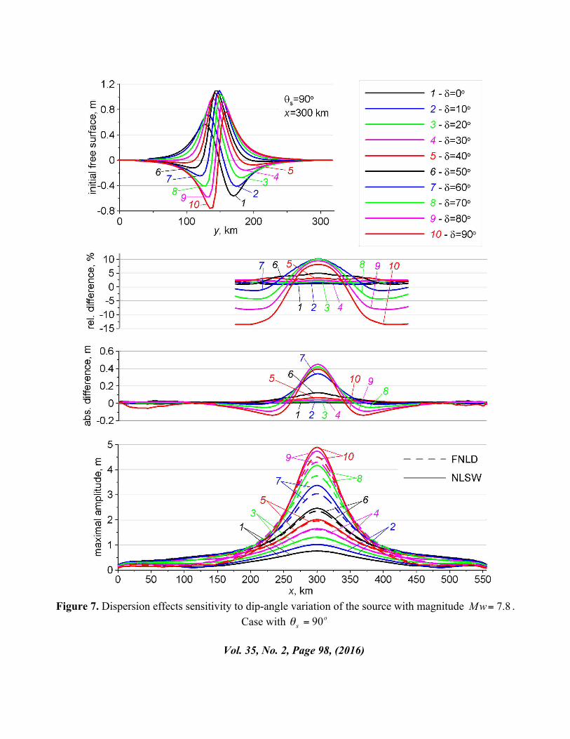
Figure 7. Dispersion effects sensitivity to dip-angle variation of the source with magnitude .

Case with

Vol. 35, No. 2, Page 98, (2016)

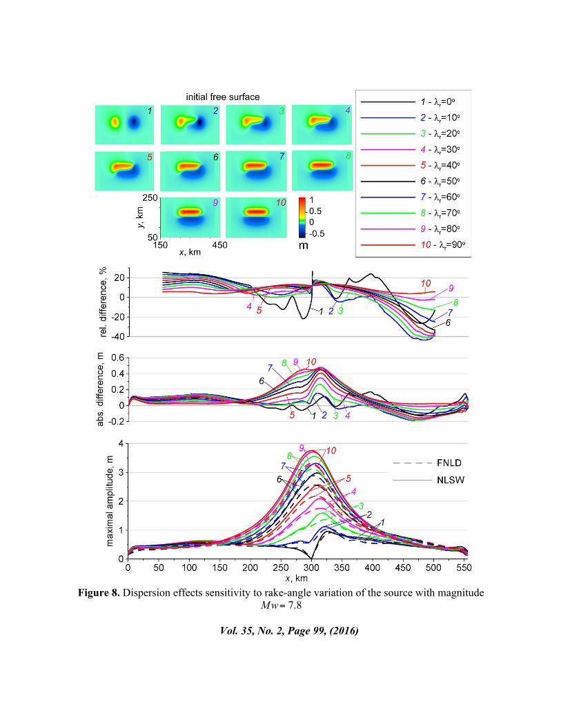
Figure 8. Dispersion effects sensitivity to rake-angle variation of the source with magnitude

Vol. 35, No. 2, Page 99, (2016)

2.4.4. Rupture depth variation for source with

Finally, we demonstrate how the dispersion sensitivity to the rupture depth of the source can be changed with consideration of the source with magnitude . For this case, the following characteristic parameters are chosen:

km, km, m.

All other parameters of the sources are the same as in item 3.2.1. The results of the computations are presented in Fig. 9. Analyzing the maximal run-ups on the wall one can note that decreasing of the rupture depth from km to km leads to the increase of the run-ups in both FNLD and NLSW computations. With further decrease of the run-up in the NLSW computations increase while in the FNLD ones decrease. For the minimal value, km, the absolute difference between this computations reaches m, and the relative one amounts Comparisons of the results of these experiments with those in item 3.2.1 show that the dispersive effects of waves generated by earthquakes with larger magnitude may be even more sensitive to the variation of the source parameters. Note that the simulations in this section are carried out in the model basin for nearfield tsunamis. Considering a far-field propagation, one should expect a significant increase of the dispersion influence. Our computations provide the qualitative results on the importance of source parameters on the dispersion effects.

2.5. Potential tsunami on a real bathymetry

In this subsection, we simulate the propagation of the tsunami generated by potential seismic source near Papua New Guinea. The parameters of the source have the following values:

km, km, , , , m, km.

The FNLD and the NLSW computations were performed on a GEBCO 1-minute grid. The computational domain lies in latitude direction from to and in longitude one from to

. The wave propagation time is set to 12 hours.

We first consider a case with the idealized bathymetry ( km) and then a real one. Thus, the simulations allow estimating the influence of the bottom irregularities on the maximal amplitude distribution and on the dispersion effects. Fig. 10 illustrates that this influence appears to be strong.

Vol. 35, No. 2, Page 100, (2016)

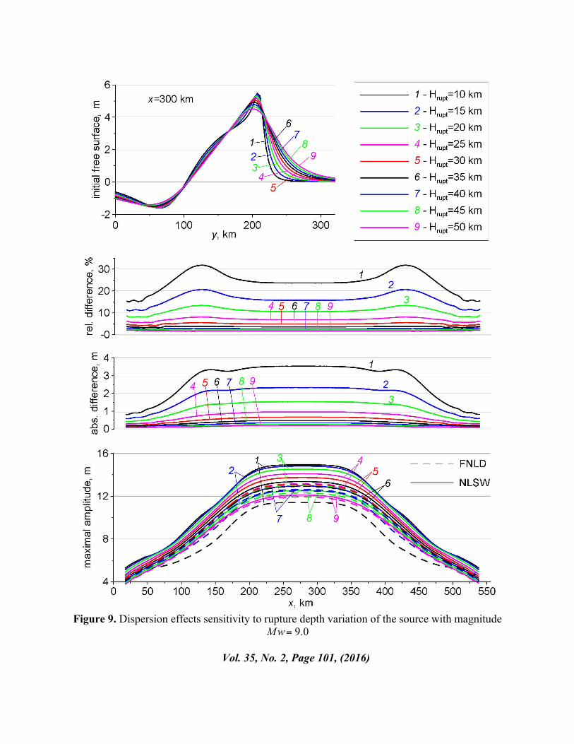
Figure 9. Dispersion effects sensitivity to rupture depth variation of the source with magnitude

Vol. 35, No. 2, Page 101, (2016)

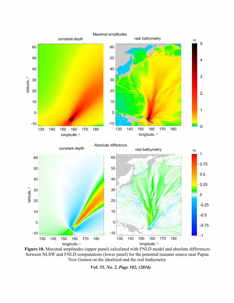
Figure 10. Maximal amplitudes (upper panel) calculated with FNLD model and absolute differences between NLSW and FNLD computations (lower panel) for the potential tsunami source near Papua

New Guinea on the idealized and the real bathymetry

Vol. 35, No. 2, Page 102, (2016)

The bottom irregularities change the direction of the maximal amplitudes and significantly complicate its pattern. The dispersion effects are generally smaller on the real bathymetry where behave complicatedly. Such behavior was observed, for example, in study (Kirby et al. 2013) during the simulation of Tohoku tsunami with using of a weakly nonlinear dispersive model. It seems that details of the bottom impact on the dispersion effects are still unclear and require further investigations. In our future work, we will consider several bottom configurations with idealized irregularities to investigate this impact.

3. CONCLUSION

In this study, we have investigated the influence of seismic source parameters on the frequency dispersion effects. These effects were estimated through the comparisons between the computations with a fully nonlinear dispersive model on a rotating sphere and with a nondispersive shallow water model. In general, the obtained results show a strong sensitivity of the dispersion effects to a rupture depth and to a dip-angle of a source. The main reason is the presence of the high frequency components in the initial surface disturbance. Counterintuitively, waves generated by sources with lager magnitude may be even more affected by dispersion. Consequently, the main factor for the dispersion manifestation is the form of the initial disturbance, but not the source extensions. Bottom irregularities may also have a significant impact on a display of dispersion. This impact will be the subject of our future investigations.

4. ACKNOWLEDGEMENTS

This research was supported by RSCF project No 14-17-00219. The authors would like to thank Gayaz Salimovich Khakimzyanov (ICT SB RAS), Leonid Borisovich Chubarov (ICT SB RAS) and Vyacheslav Konstantinovich Gusiakov (ICMMG SB RAS, ICT SB RAS) for their valuable comments on the manuscript.

Vol. 35, No. 2, Page 103, (2016)

REFERENCES

Cherevko A.A. and Chupakhin A.P. (2009). Equations of the shallow water model on a

rotating attracting sphere.1. Derivation and general properties. J. Appl. Mech. Tech. Phys. Vol. 50, No 2. P 188–198.

Chubarov L.B. and Guslakov V.K. (1985). Tsunamis and earthquake mechanisms in the island arc regions // Science of Tsunami Hazards. Tsunami Society, Honolulu, USA. Vol. 3, No 1. P. 3–21.

Dao M.H. and Tkalich P. (2007). Tsunami propagation modelling — a sensitivity study. Nat. Hazards Earth Syst. Sci. Vol. 7. P. 741–754.

Didenkulova I.I., Pelinovsky E.N. and Didenkulov O.I. (2014). Run-up of long solitary waves of different polarities on a plane beach. Izv. Atmos. Oceanic Phys. Pleiades Publishing. Vol. 50, No 5. 532–538.

Fedotova Z.I. and Khakimzyanov G.S. (2010). Nonlinear-dispersive shallow water equations on a rotating sphere. Russian Journal of Numerical Analysis and Mathematical Modelling. De Gruyter. Vol. 25, No 1. P. 15–26.

Fedotova Z.I. and Khakimzyanov G.S. (2014). Nonlinear-dispersive shallow water equations on a rotating sphere and conservation laws. Journal of Applied Mechanics and Technical Physics. Springer. Vol. 55, No 3. P. 404–416.

Fedotova Z.I., Khakimzyanov G.S. and Gusev O.I. (2015). History of the development and analysis of numerical methods for solving nonlinear dispersive equations of hydrodynamics. I. One-dimensional models problems. Computational Technologies. Russia, ICT SB RAS. Vol. 20, No 5. P. 120–156 (In Russian).

Glimsdal, S., Pedersen G.K., Harbitz C.B. and Lovholt F. (2013). Dispersion of tsunamis: does it really matter? Nat. Hazards Earth Syst. Sci. Vol. 13. P. 1507–1526.

Gusev O.I. (2012). On an algorithm for surface waves calculation within the framework of nonlinear dispersive model with a movable bottom. Computational technologies. Russia, ICT SB RAS. Vol. 17, No. 5. P. 46–64 (In Russian).

Gusev O.I. (2014). Algorithm for surface waves calculation above a movable bottom within the frame of plane nonlinear dispersive model. Computational technologies. Russia, ICT SB RAS. Vol. 19, No 6. P. 19–41 (In Russian).

Gusev O.I. and Khakimzyanov G.S. (2015). Numerical simulation of long surface waves on a rotating sphere within the framework of the full nonlinear dispersive model. Computational Technologies. Russia, ICT SB RAS. Vol. 20, No 3. P. 3–32 (In Russian).

Gusev O.I., Shokina N.Y., Kutergin V.A. and Khakimzyanov G.S. (2013). Numerical modelling of surface waves generated by underwater landslide in a reservoir. Computational technologies. Russia, ICT SB RAS. Vol. 18, No 5. P. 74–90 (In Russian).

Gusiakov V.K. (1978). Static displacement on the surface of an elastic space. Ill-posed problems of mathematical physics and interpretation of geophysical data. Novosibirsk, VC SOAN SSSR. P. 23–51 (in Russian).

Vol. 35, No. 2, Page 104, (2016)

Horrillo J., Grilli S.T., Nicolsky D., Roeber V., Zhang J. (2015). Performance benchmarking

tsunami models for NTHMP’s inundation mapping activities. Pure Appl. Geophys. Vol. 172, No. 3–4. P. 869–884.

Kajiura K. (1963). The leading wave of a tsunami. Bull. Earthq. Res. Inst. Vol. 41. P. 535–571. Khakimzyanov G.S., Gusev O.I., Beisel S.A., Chubarov L.B. and Shokina N.Yu. (2015).

Simulation of tsunami waves generated by submarine landslides in the Black Sea. Russian Journal of Numerical Analysis and Mathematical Modelling. De Gruyter. Vol. 30, No 4. P. 227–237.

Khakimzyanov G.S., Shokin Yu.I., Barakhnin V.B. and Shokina N.Yu. (2001). Numerical modelling of fluid flows with surface waves. Publishing House of SB RAS, Novosibirsk (In Russian).

Kirby J.T., Shi F., Tehranirad B., Harris J.C. and Grilli S.T. (2013). Dispersive tsunami waves in the ocean: Model equations and sensitivity to dispersion and Coriolis effects. Ocean Modelling. Vol. 62. P. 39–55.

Kosykh V.S., Chubarov L.B., Gusiakov V.K., Kamaev D.A., Grigor’eva V.M. and Beisel S.A. (2013). A technique for computing maximum heights of tsunami waves at protected Far Eastern coastal points of the Russian Federation. Results from Testing of New and Improved Technologies, Models, and Methods of Hydrometeorological Forecasts. IG SOTsIN, Moscow–Obninsk. No 40, P. 115–134 (In Russian).

Lovholt F., Pedersen G.K. and Gisler G. (2008). Oceanic propagation of a potential tsunami from the La Palma Island. J. Geophys. Res. Vol. 113. C09026.

Lynett P.J. and Liu P.L.-F. (2002). A numerical study of submarine-landslide-generated waves and run-up. Proc. Royal Society of London. A. Vol. 458. P. 2885–2910.

Okada Y. (1985). Surface deformation due to shear and tensile faults in a half space. Bull. Seism. Soc. Am. Vol. 75. P. 1135–1154.

Pelinovsky E.N. (1996). Hydrodynamics of tsunami waves. Institute of Applied Physics RAS, Nizhny Novgorod (In Russian).

Shi F, Kirby J.T., Harris J.C., Geiman J.D., Grilli S.T. (2012). A high-order adaptive time-stepping TVD solver for Boussinesq modeling of breaking waves and coastal inundation. Ocean Modelling. Vol. 43–44. P. 36–51.

Shokin Yu.I., Babailov V.V., Beisel S.A., Chubarov L.B., Eletsky S.V., Fedotova Z.I., Gusiakov V.K. (2008). Mathematical Modeling in Application to Regional Tsunami Warning Systems Operations. Notes on Numerical Fluid Mechanics and Multidisciplinary Design. Berlin: Springer. Vol. 101: Computational Science and High Performance Computing III. P.52–68.

Tadepalli S. and Synolakis C.E. (1994). The runup of N-waves. Proc. Royal Soc. London. A445. P. 99–112.

Titov V. and Synolakis , C.E. (1995). Evolution and runup of breaking and nonbreaking waves using VTSC2. Journal of Waterway, Port, Coastal and Ocean Engineering. Vol. 126, No 6. P. 308–316.

Vol. 35, No. 2, Page 105, (2016)