Scientific Computing forX-Ray Computed Tomography

Artifacts and Model Calibration

Martin S. AndersenSection for Scientific Computing

DTU Compute

DTUJanuary 19, 2017

Reconstruction Model

Model assumptions may be flawed or unwarranted

I reconstruction geometry

I calibration errors (white field is estimated)

I source spectrum, energy dependent attenuation

I detector model, nonlinearities (e.g., saturation)

I object motion, vibrations, dynamic process

I noise model

Model versus physics

I Physics → measurements

I Measurements → model+algorithm → reconstruction

1/19

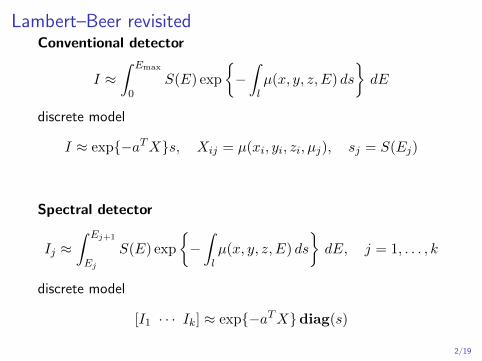
Lambert–Beer revisitedConventional detector

I ≈∫ Emax

0S(E) exp

{−∫lµ(x, y, z, E) ds

}dE

discrete model

I ≈ exp{−aTX}s, Xij = µ(xi, yi, zi, µj), sj = S(Ej)

Spectral detector

Ij ≈∫ Ej+1

Ej

S(E) exp

{−∫lµ(x, y, z, E) ds

}dE, j = 1, . . . , k

discrete model

[I1 · · · Ik] ≈ exp{−aTX}diag(s)

2/19

X-ray attenuation

X-ray attenuation is primarily a function of

I X-ray energy

I atomic number of the material being imaged

I material density

Higher-energy X-rays

I penetrate more effectively than lower-energy ones

I are less sensitive to changes in material density andcomposition

Very different densities and/or atomic constituents → easy todifferentiate

3/19

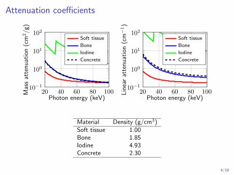
Attenuation coefficients

20 40 60 80 10010−1

100

101

102

Photon energy (keV)

Mas

sat

ten

uat

ion

(cm

2/g

)

Soft tissue

Bone

Iodine

Concrete

20 40 60 80 10010−1

100

101

102

Photon energy (keV)

Lin

ear

atte

nu

atio

n(c

m−1)

Soft tissue

Bone

Iodine

Concrete

Material Density (g/cm3)Soft tissue 1.00Bone 1.85Iodine 4.93Concrete 2.30

4/19

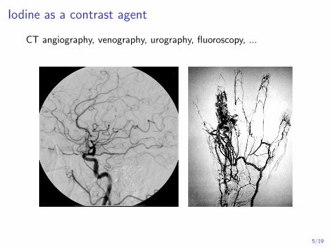
Iodine as a contrast agent

CT angiography, venography, urography, fluoroscopy, ...

5/19

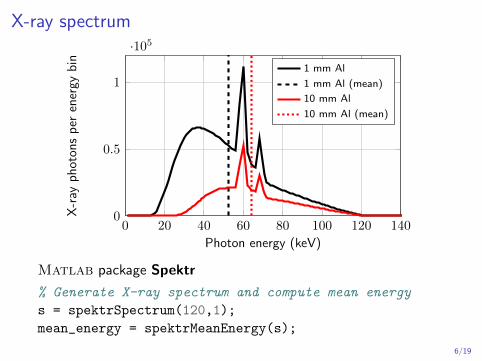
X-ray spectrum

0 20 40 60 80 100 120 1400

0.5

1

·105

Photon energy (keV)

X-r

ayp

hot

ons

per

ener

gyb

in1 mm Al

1 mm Al (mean)

10 mm Al

10 mm Al (mean)

Matlab package Spektr

% Generate X-ray spectrum and compute mean energy

s = spektrSpectrum(120,1);

mean_energy = spektrMeanEnergy(s);

6/19

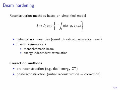
Beam hardening

Reconstruction methods based on simplified model

I ≈ I0 exp

{−∫lµ(x, y, z) ds

}

I detector nonlinearities (onset threshold, saturation level)I invalid assumptions

I monochromatic beamI energy-independent attenuation

Correction methods

I pre-reconstruction (e.g. dual energy CT)

I post-reconstruction (initial reconstruction + correction)

7/19

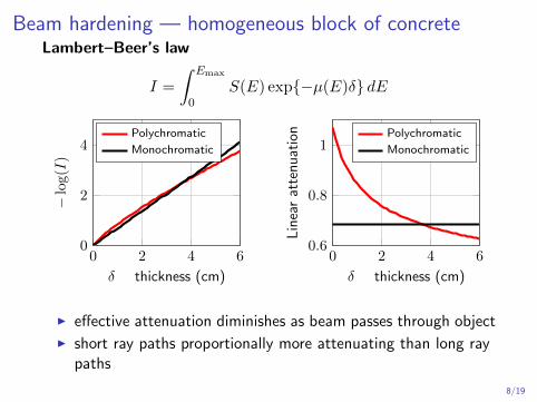
Beam hardening — homogeneous block of concreteLambert–Beer’s law

I =

∫ Emax

0S(E) exp{−µ(E)δ} dE

0 2 4 60

2

4

δ thickness (cm)

−lo

g(I

)

Polychromatic

Monochromatic

0 2 4 60.6

0.8

1

δ thickness (cm)L

inea

rat

ten

uat

ion Polychromatic

Monochromatic

I effective attenuation diminishes as beam passes through object

I short ray paths proportionally more attenuating than long raypaths

8/19

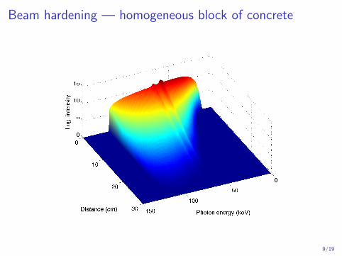
Beam hardening — homogeneous block of concrete

9/19

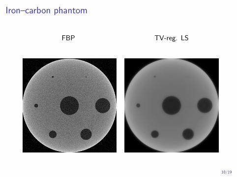
Iron–carbon phantom

FBP TV-reg. LS

10/19

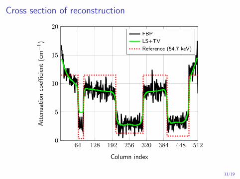
Cross section of reconstruction

64 128 192 256 320 384 448 5120

5

10

15

20

Column index

Att

enu

atio

nco

effici

ent

(cm

−1)

FBP

LS+TV

Reference (54.7 keV)

11/19

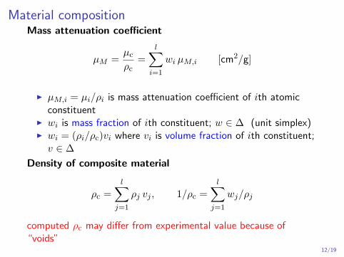
Material compositionMass attenuation coefficient

µM =µcρc

=

l∑i=1

wi µM,i [cm2/g]

I µM,i = µi/ρi is mass attenuation coefficient of ith atomicconstituent

I wi is mass fraction of ith constituent; w ∈ ∆ (unit simplex)I wi = (ρi/ρc)vi where vi is volume fraction of ith constituent;v ∈ ∆

Density of composite material

ρc =

l∑j=1

ρj vj , 1/ρc =

l∑j=1

wj/ρj

computed ρc may differ from experimental value because of“voids”

12/19

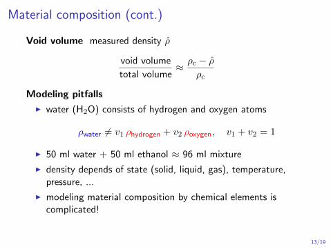
Material composition (cont.)

Void volume measured density ρ̂

void volume

total volume≈ ρc − ρ̂

ρc

Modeling pitfalls

I water (H2O) consists of hydrogen and oxygen atoms

ρwater 6= v1 ρhydrogen + v2 ρoxygen, v1 + v2 = 1

I 50 ml water + 50 ml ethanol ≈ 96 ml mixture

I density depends of state (solid, liquid, gas), temperature,pressure, ...

I modeling material composition by chemical elements iscomplicated!

13/19

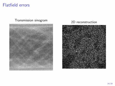
Flatfield errors

Transmission sinogram2D reconstruction

14/19

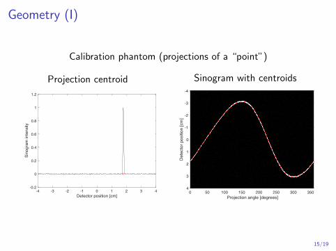
Geometry (I)

Calibration phantom (projections of a “point”)

Projection centroid

-4 -3 -2 -1 0 1 2 3 4Detector position [cm]

-0.2

0

0.2

0.4

0.6

0.8

1

1.2

Sino

gram

inte

nsity

Sinogram with centroids

0 50 100 150 200 250 300 350Projection angle [degrees]

-4

-3

-2

-1

0

1

2

3

4

Det

ecto

r pos

ition

[cm

]

15/19

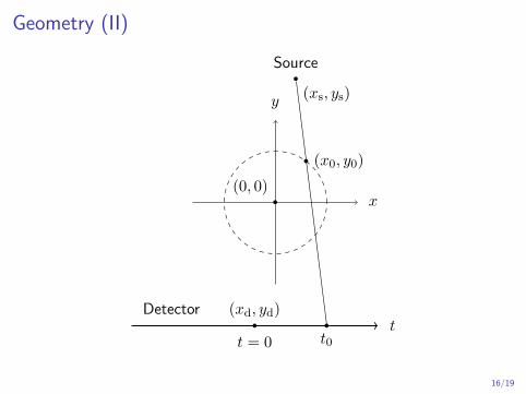
Geometry (II)

(0, 0)

(xs, ys)

(xd, yd)

Source

t = 0

(x0, y0)

Detectort

x

y

t0

16/19

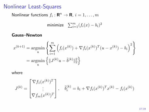
Nonlinear Least-Squares

Nonlinear functions fi : Rn → R, i = 1, . . . ,m

minimize∑m

i=1(fi(x)− bi)2

Gauss–Newton

x(k+1) = argminu

{m∑i=1

(fi(x

(k)) +∇fi(x(k))T (u− x(k))− bi)2}

= argminu

{‖J (k)u− b̃(k)‖22

}where

J (k) =

∇f1(x(k))T

...

∇fm(x(k))T

, b̃(k)i = bi +∇fi(x(k))Tx(k) − fi(x(k))

17/19

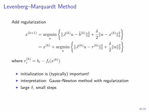
Levenberg–Marquardt Method

Add regularization

x(k+1) = argminu

{‖J (k)u− b̃(k)‖22 +

δ

2‖u− x(k)‖22

}= x(k) + argmin

u

{‖J (k)u− r(k)‖22 +

δ

2‖u‖22

}where r

(k)i = bi − fi(x(k))

I initialization is (typically) important!

I interpretation: Gauss–Newton method with regularization

I large δ, small steps

18/19

References I

[Lev44] K. Levenberg. “A Method for the Solution of Certain Non-LinearProblems in LEast Squares”. In: Quarterly of Applied Mathematics2.2 (1944), pp. 164–168. url:http://www.jstor.org/stable/43633451.

[Mar63] D. W. Marquardt. “An Algorithm for Least-Squares Estimation ofNonlinear Parameters”. In: Journal of the Society for Industrialand Applied Mathematics 11.2 (June 1963), pp. 431–441. doi:10.1137/0111030. url: https://doi.org/10.1137/0111030.

[Gul+87] G. T. Gullberg et al. “Estimation of geometrical parameters for fanbeam tomography”. In: Physics in Medicine and Biology 32.12(1987), p. 1581. url:http://stacks.iop.org/0031-9155/32/i=12/a=005.

[NW06] J. Nocedal and S. J. Wright. Numerical Optimization. 2nd.Springer, 2006.

19/19