Professor: prof. dr. ir. J.J. Kok

Adaptive Computed Torque Computed Reference Control of a flexible RT-manipulator

Theoretical analysis, simulations and experiments

Eric Tenbult

Coaches: dr. ir. F.E. Veldpaus and ir. P.C. Mulders

WFW, Control and identification of mechanical systems Department of Mechanical Engineering, Eindhoven University of Technology

Report no.: 93.178

Abstract.

Abstract

In mechanical systems the presence of deformable subsystems Goints) is responsible for an increase of the number of generalized coordinates, i.e. the number of independent coordinates necessary and sufficient to adequately describe the configuration of the system at each time. Consequently the number of degrees of freedom to be controlled Istabilized exceeds the number of control inputs. Furthermore, the desired trajectories of the generalized coordinates are not determined uniquely by the output trajectory. A possibility to tackle this problem, is to apply a Computed Torque Computed Reference Control law, which incorporates nonlinear flexible robot dynamics and computes both the input torques and the a priori unknown references for the generalized coordinates. The controller design according to this algorithm is capable of accomplishing a reasonable trajectory tracking, while keeping the elastic vibrations bounded. Based on Lyapunov's second method global stability is ensured. regardless of the magnitude of the joint stiffness.

In order to improve the performance if some system parameters are unknown an adaptive version of the control law has been derived. Besides the familiar direct adaptation algorithm which extracts parameter information from the tracking errors, a new technique called composite adaptive control has been introduced. This new algorithm extracts parameter information from tracking errors as well as from prediction errors and leads to faster adaptation without incurring significant oscillation in the estimated parameters. thus yielding improved performance. However. both adaptation methods require linear parametrization of the system dynamics.

To illustrate the qualities of the designed controller several simulations under various conditions have been performed on a flexible RT-manipulator model. Although stability combined with asymptotic tracking can only be ensured for simulations with a perfect model, reasonable results can be obtained for the practical situation with time discrete implementation. actuator saturation, measurement noise etc. Similar characteristics and robustness properties can be obtained if the control law is implemented on a real RT­manipulator. Therefore adaptive CTCRC is considered to be a suitable approach for the control of nonlinear mechanical systems with more degrees of freedom than input signals and with uncertain parameters.

Content8.

Contents

Abstract Contents Notation

Chapter 1 Introduction ........................................... 1

Chapter 2 2.1 2.2

Chapter 3 3.1 3.2

Control of flexible robots ................................ 2 The model .............................................. 2 Adaptive Computed Torque Computed Reference Control .......... 3 2.2.1 Stability ... . . . . . . . . . . . . . . . . . . . . . . . . . . . . . . . . . . 5 2.2.2 Direct adaptation algorithm ...................... 6 2.2.3 Composite adaptation algorithm . . . . . . . . . . . . . . . . . . . 7 2.2.4 Adaptive CTCRC in component form ............... 8

Simulations .......................................... 12 The RT-robot ........................................... 12 Simulations ............................................ 13 3.2.1 Variation of spring constant ..................... 15 3.2.2 Direct and composite adaptation. . . . . . . . . . . . . . . . . . 17 3.2.3 Weak differentiation . . . . . . . . . . . . . . . . . . . . . . . . . . . 19 3.2.4 Discrete-time simulations ....................... 21 3.2.5 Supplementary practical conditions ............... 22

Chapter 4 Experiments.......................................... 25

Chapter 5 Conclusions and recommendations ...................... 29

Bibliography .................................................... 31

Appendices Appendix A: Appendix B: Appendix C: Appendix D:

Equations of motion of aRT-robot ................ 32 Variant of adaptive CTCRC ..................... 35 Discrete-time differentiation ..................... 36 Dynamical model DC-motor ..................... 38

Notation.

Notation

a, a, as .!!. A aT AT - , A -1

A (iJ) ci a a (n)

d d la I '-f(t) g*g(t)

: scalars : vector : matrix : transposition : inversion : element of matrix A on row i , column j : fIrst order time derivative of a : second order time derivative of a : n'th order time derivative of a : estimate of a :d-a : norm of a : , is a function of argument t : g is not a function of argument t

Chapter 1: Introduction. 1

Chapter 1 Introduction

In order to increase operating speeds, modern robots should be lightweight constructions to reduce the driving torques and to enable the robot to respond faster. This however withdraws the assumption that the links behave as rigid bodies and the transmissions are stiff. Deformation ofthe links is usually of minor importance compared to the deformation in the joints and for this reason link deformation is omitted. Joint elasticity usually results in lightly damped oscillations which may cause stability problems if the flexibility is neglected in the control system. In order to avoid instability a control design model which accounts for the flexibilities is required. As a consequence of the availability of low cost powerful microprocessors realtime application of more complex control algorithms is possible nowadays.

During the last decade, several control algorithms for flexible manipulators have been developed. One possible approach to control flexible robots is feedback linearization combined with pole placement of the feedback linearized system. Major drawbacks of this method are the large computation time and the requirement for a very accurate model of the system. Another approach is to apply a method which is based on singular perturbation techniques. However, these techniques are restricted to robots with elastic joints only, while global stability is guaranteed for small flexibilities only [Lammerts et aI.,1993].

Recently an alternative has been developed at the Eindhoven University of Technology which is based on the familiar computed torque control law. The original version relies on the assumption that all manipulator elements are perfectly rigid and that the number of actuator inputs equals the number of degrees of freedom. Therefore, the presence of flexibilities results in less tracking accuracy and can even lead to instability. In order to improve the performance of a flexible manipulator, the controller must achieve both reasonable trajectory tracking and stabilization of the elastic deflections. A new so-called (adaptive) Computed Torque Computed Reference Control algorithm ensures stability combined with asymptotic tracking for a flexible robot with both joint elasticity and link flexibility regardless of the magnitude of the flexibility. If the system parameters or the payload parameters are unknown, an adaptive version can be used such that trajectory tracking is achieved while all signals within the system remain bounded.

The purpose of the research in this report is to get an impression of the properties of the adaptive CTCRC algorithm. Chapter 2 presents the theoretical analysis of the designed controller. Besides the proof of stability two (on-line) adaptive control schemes have been derived. These schemes are based on the assumption that the structure of the mathematical model is correct, but that some of the model parameters are unknown. Furthermore, it is assumed that these parameters are constant and that the model is linear in these parameters. Chapter 3 presents the simulation results of a flexible RT­manipulator, controlled with an adaptive CTCRC law. The issue of robustness has been examined by performing several simulations under practical conditions. Chapter 4 gives a survey ofthe experimental results that are obtained by implementing adaptive CTCRC, PD-control and computed torque control on a real RT-manipulator. Chapter 5 offers brief concluding remarks and recommendations.

Chapter 2: Control of flexible robots. 2

Chapter 2 Control of flexible robots

2.1 The model

The manipulators considered in this report can be modeled as an open chain of n rigid links connected by cylindrical, revolute or prismatic joints with one degree of freedom per joint. Several links, however, are driven via an elastic transmission. The base of the manipulator is fIXed to the ground while the other end with gripper and payload has to follow a prescribed trajectory. Motor dynamics will not be taken into consideration.

The main difference between a flexible manipulator and its rigid counterpart consists of the fact that the number of degrees of freedom (n +e) to be controlled / stabilized is unequal to the number of actuators (n). The number of extra generalized coordinates (e ) for the flexible systems in this report equals the number of elastic transmissions. Neglecting this extra degree(s) of freedom can lead to instability.

The equations of motion (a set of second order differential equations) can be derived by the Lagrange formalism. In general the dynamical model of a flexible manipulator can be written in the following standard form. It is assumed that the model perfectly matches reality when the parameters are correct. These parameters are considered to be constant or at least changing much slower than the generalized coordinates.

Here !L(t) E R (n-e) is a vector of generalized coordinates, necessary and sufficient to describe the robot configuration, 12. E R m is a vector of constant, unknown system parameters, M<IL1l)E R (n-e).Cn-e) is a symmetric positive definite inertia matrix, C<rLtLJi)E R(n+e)x(n+e) is a matrix which accounts for the Coriolis and centrifugal torques while If.<rLtLJi)E R(n+el is a vector which accounts for an eventual external loading (e.g. by gravity) and for all internal torques except actuator torques. These internal torques are due to, for instance damping, friction and joint flexibility. H(g)E R (n+e)xn is a distribution matrix with full rank and u ERn is a vector of actuator forces. The output vector l..(t)E R 8 is a smooth bounded vector function of the generalized coordinates.

The given model is applicable for a broad class of flexible manipulators. The matricesM and C are not independent since (!VI -2C) is skew-symmetric. This implies that at all times tL T(!VI - 2C)Q:, "" O. Often the vector If.<rLfLll..,t) can be written as the sum of a stiffness term K!L, a viscous damping term Btl and a term which represents the remaining internal torques, Coulomb friction for instance.

(2.2)

Chapter 2: Control of flexible robots. 3

Here B(J!)E R (n .... )"(n .... ) is a (semi-) positive defInite damping matrix, K E R (n+e).(n+e) is a semi­positive defInite stiffness matrix and lI.. (!1lLJ2,;t)E R (n+e) is a vector with the remaining forces. A major restriction of this choice is the assumption that the components of K are exactly known, since K:FKCiiJ.

In general, the output (gripper) trajectory l!.(t) is a smooth function of the generalized coordinates l!. =h(g). However, for a flexible manipulator only n coordinates of the vectorQ.(t) can be determined from the output trajectory l!.(t). These coordinates are the components of a vector Q.k' Now it is possible to partition Q.(t) in two components:

(2.3)

where [Lk

Lu]E R (n+e),,(n+e) is a permutation matrix, Q. E R It is a vector with those components of Q.(t) that are determined from y(t) whill Q. ERe is a vector with those components of g.,(t) that cannot be determined from y(t). The index d denotes a desired trajectory.

The components of Q. can be determined from the output equation if l!.(t) is replaced by the desired output tr~ectory l!. (t). This is not possible for Q. . However, it is assumed that it is possible to compute a gmooth and bounded trajectoryudQ. . The determination of such a trajectory is one of the topics of section 2.2.4. ud

2.2 Adaptive Computed Torgue Computed Reference Control

The goal of a controller for a flexible manipulator is to achieve trajectory tracking and to limit the occurring vibrations between acceptable bounds. The control law described in this report is based on a model of the flexible manipulator in order to compensate for non­linearities and to guarantee a desired closed loop behaviour.

Good trajectory tracking is achieved if the position error g, =Q. -Q. and its derivative ~ remain bounded and converge to zero. This condition can 'be reformulated by the introduction of a virtual reference trajectory Q. (t) with:

r

(2.4)

where, AE R (n • .,).(n+e) is a positive defInite (diagonal) matrix. Since e is defined as g,r ""Q. -Q. and consequently ~ =~ + Ag" the requirements with respect to g, and ~ are fulfilfed if e ~ 0 for t ~ 00. The definition of e can be viewed as a stable first-order differential-equation in e, with e as an input. -r

- -r

Chapter 2: Control of flexible robots. 4

The control problem now is to derive an algorithm which guarantees that ~ --t Q for t --t 00. In accordance with the basic algorithm of Slotine and Li the next controf law has been chosen:

where b.. E R'" is a vector of estimated system parameters and KrE R (n<e)x(n<e) is a positive defInite diagonal gain matrix. The control algorithm consists of two components i.e. a full dynamics feedforward compensation part and a feedback part K£ . Besides for the computation of u(t), this control law is also used to determine the unknown part fL of fL =LJ1.. + Lu9.. from the set of equations (2.5). ur r kr ur

This control law can also be analyzed according to the sliding control methodology. Therefore, e =e +Ae =0 is considered to be a set of (n+e) sliding surfaces, such that sliding mode occurs

ron-the1ntersection of planes eri""ei + Af!i with i =1..(n+e). The dynamics while

in sliding mode e =0 can be written as: -r -

e =0 (2.6) -r -

By solving the above equation formally for the control input an expression for u called the equivalent control u can be obtained, which can be interpreted as the continuous control law that would main'iain !1.. =Q if the dynamics were exactly known. For simplicity only the non-adaptive case is considered. Substitution of the equations of motion (1.1) in e =ii -ii + Ae yields: -r ::t....d::t.... -

e =ii - M -l(Hu -Cn -Bn -Krr -IT ) + Ae -r ::t....d _::t....::t....::t.... o..n -

(2.7)

Since Hu is defIned as Hu =Hu(e ",,0) following equation can be obtained: -eq -eq - -r -

Hu =Hu + Ce +Ke +Ke - -eq -r -r r-r

(2.8)

Now, it is obvious that Hu is cor;osed of a term which keeps the system in sliding motion and a PI part (C+K ~ +K e dt which forces the system to the sliding surface e ... 0. Substitution of the co~froll -in the equation (2.6) yields the error equation of the non:adaptive closed-loop system:

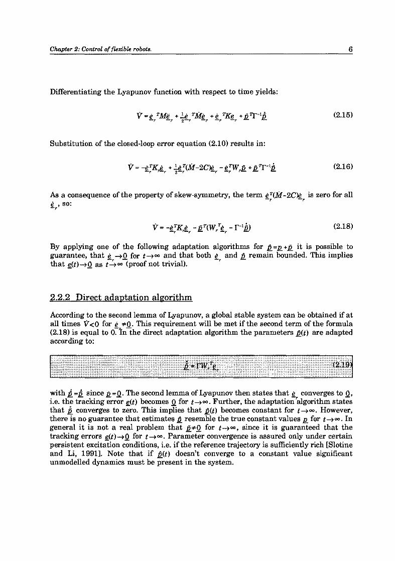
Me +Ce +Ke +Ke =0 -r -r -r r.-..r-(2.9)

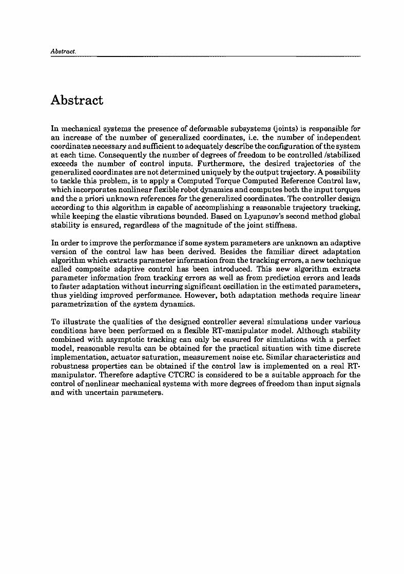
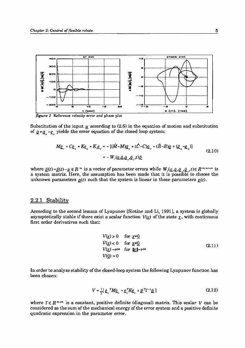
A possible solution of this differential equation combined with a phase plot is given in fIgure 1. Note that e (t) intersects the sliding surface several times. Further details about this simulation will 'be given in section 3.2.

Chapter 2: Control of flexible robots.

i '"it' ~ • "

400

300

aoo

100

0

-100

-aoo o

.,. clO't

I J I

±± ! I: !

:

_. ······t················t-·_-+-10 HI 20

figure 1 Reference velocity error and phase plot

5

-0

i ....................... i .. _ ................. ~ ................ --.. .

! i ; !

-'8~----~------~------~. -10 -8 0 8

-10

• [rn]. [ .... a]

Substitution of the input u according to (2.5) in the equation of motion and substitution of fL ""'fLr -tr yields the error equation of the closed loop system:

Me + Ce + Ke + Kp "" - [(M"-M)n + (C-C)n + CfJ-B\;' + (A -t7 )] -r -r -r,c:;..r :.t.r ::L.r ~ \5..1t c..n (2.10)

where fJ..(t) ""'fJ..(t) -11. ER m is a vector of parameter errors while Wr{g"tJ..,fL ,tl. ,t)E R<rt+e)om is a system matrix. Here, the assumption has been made that it is possIble to choose the unknown parameters 11.(t) such that the system is linear in those parameters 11.(t).

2.2.1 Stability

According to the second lemma of Lyapunov [Slotine and Li, 1991], a system is globally asymptotically stable if there exist a scalar function VW of the state ~, with continuous first order derivatives such that:

V~»O

VW<O VW~oo

V@ =0

for ~*Q for~

for k.1~oo (2.11)

In order to analyze stability ofthe closed-loop system the following Lyapunov function has been chosen:

(2.12)

where r E R mom is a constant, positive definite (diagonal) matrix. This scalar V can be considered as the sum of the mechanical energy of the error system and a positive definite quadratic expression in the parameter error.

Chapter 2: Control of {krlbk robots. 6

Differentiating the Lyapunov function with respect to time yields:

(2.15)

Substitution of the closed-loop error equation (2.10) results in:

(2.16)

As a consequence of the property of skew-symmetry, the term eT(..M-2C)e is zero for all -r -r e ,so:

-r

(2.18)

By applying one of the following adaptation algorithms for b., =11. +Ji. it is possible to guarantee, that tr -t,Q, for t-t oo and that both tr and b., remain bounded. This implies that ~(t)-tQ as t-t OO (proof not trivial).

2.2.2 Direct adaptation algorithm

According to the second lemma of Lyapunov, a global stable system can be obtained if at all times V <0 for e *0. This requirement will be met if the second term of the formula (2.18) is equal to O:-'in the direct adaptation algorithm the parameters b.,(t) are adapted according to:

with il. =Q since il. =Q. The second lemma of Lyapunov then states that t converges to Q, i.e. the tracking error e(t) becomes 0 for t-too. Further, the adaptation ralgorithm states that Q converges to zero. This implies that b.,(t) becomes constant for t-t oo . However, there is no guarantee that estimates b., resemble the true constant values 11. for t-too. In general it is not a real problem that Ji.*Q for t-t OO , since it is guaranteed that the tracking errors ~(t)-tQ for t-too. Parameter convergence is assured only under certain persistent excitation conditions, i.e. if the reference trajectory is sufficiently rich [Slotine and Li, 1991]. Note that if b.,(t) doesn't converge to a constant value significant unmodelled dynamics must be present in the system.

Chapter 2: Control of flexible robots. 7

2.2.3 Composite adaptation algorithm

Parameter estimation is based on extracting information from available system data, by using an estimation model. This estimation model doesn't have to be the same as the model used for control purpose. A fairly general model for parameter applications is in the linear parametrization form:

~(t) "" Y(t)12.. (2.20)

where ~E R k is a vector containing the outputs of the system, 12.. E R m the parameter vector and Y(t)E R kxm is a signal matrix. It is obvious at this point that the output vector of the estimation model doesn't have to be the same as the output in a control problem.

A possible approach to obtain a suitable estimation model is to reformulate the equations of motion.

Hu -KY.,. ... M!i. +CtL + BtL +H.n

Hu - KY.,. "" Y m <!LtJ...Ii..,t)12.. +J!.m <!LtJ...IJ.,t) (2.21)

~m (!lil...IJ.,t) ... [H u - Kfl. - Ym

] ... Y m <!I...!J..,!i...t) J2..

Note that z(t) and Y(t) are required to be known from continuous measurement of the system si~als. Since 12.. is a constant parameter vector and equation (2.21) must hold for all t, the estimation model is an overdetermined set of equations. Now it is possible to predict the value of ~(t) at time t, by substituting the parameter estimate h.,(O in equation (2.20). This yields:

~(t) "" Y(t)h.,(t) (2.22)

where :(t) is the predicted value at time t. The difference between the predicted output and the measured output is called the prediction error, denoted bye (t), i.e.:

-p

e (t) "" i(t) - z(t) -p - -

(2.23)

Now, a relation between the prediction error and the parameter error can be obtained.

~)t) ... Y(t)h.,(t) - Y(t)J2.. ... Y(t)Q (2.24)

Chapter 2: Control of fle:rible robots. 8

In order to reduce the prediction error, it is possible to derive a (gradient) estimator which updates the parameters in the converse direction of the gradient of the squared prediction error, with respect to the parameters:

(2.25)

This equation is equivalent with:

(2.26)

According to [Slotine and Li, 1991], it is possible to derive an adaptation algorithm which extracts information about the parameters from the tracking errors e (t), as well as from the prediction errors e . This so-called composite adaptation algorithm can further improve the performance ofthe adaptive controller. A combination of the direct adaptation algorithm and the gradient estimator leads to following composite adaptation algorithm:

This adaptation law simply adds an extra term in the expression of V (2.18).

(2.28)

Now, the second lemma of Lyapunov states that both the tracking errors e (t) and the prediction errors e converge to o. Similar to the direct algorithm, the composite adaptation law only~arantees that~(t)-+.Q. for t-+ oo • Ifin addiction, the trajectories are persistently exciting and uniformly continuous, the estimated parameters asymptotically converge to the true parameters.

2.2.4 Adaptive CTCRC in component form

So far it is assumed that f1.. =L,o. + Luf1. is completely known. However, the trajectory f1.. is unknown beforehand. Withou\dloss ortgenerality it is possible to write the equations o'f motion for a manipulator with elastic joints,

(2.30)

Chapter 2: Control of flerible robots. 9

in component form as

o l~8 [0 0 o !l..e + 0 K

B' O-K u !l..u

where !l.. T = £!l.. T !l.. T] ERn is a vector of generalized link coordinates, !l.. E R (n-e) is a vector of link cooldinatese with a stiff transmission, !l.. ERe is a vector of link coordinates with an elastic transmission and !l.. ERe is a vector of coordinates necessary and sufficient to describe the deformation of'the elastic transmission (motor coordinates). u E R (n-e) is a vector component of u directly acting on !l.. ' while u is a vector component of u acting on!l.. via an elastic transmission. 8 -e -

e

For a further elaboration the adaptive Computed Torque Computed Reference Control algorithm,

is formulated in component form as

!!8 =[M88 Mse]!ikr +[C88 Cse]tLkr +Bg" +g8 + Kr&."r

Hu = Q = [Me" Mee]!ikr + [Ces Cee]tLkr + BefLe + K{!J..er -!l..) + 8..e + KrJ..er

U =M Ii +13;, -K(" -n )+A- +K e -e Uu::Lur u.:s.u '!t.er ::I.. ur 6..u ru.;;..ur

(2.32)

(2.33)

where !l.. T = £!l.. T !l.. T] ERn is a vector of link reference coordinates,!l.. E R (n-e) is a vector of stiff llnltreferenCe coordinates,!l.. ERe is a vector of elastic link "reference coordinates and!l.. ERe is a vector of motor teference coordinates. ur Characteristic for this control law is the on-line determination of!l.. from the second set of equations. This gives: ur

n = K -l{ rM M L + [c C L + 13;, + A- + K e } + n .1iLur t 418 eeJLkr ell eeJLkr e::Le 6.41 r=er .1iLer

(2.34)

Chapter 2: Control of {lerible robots. 10

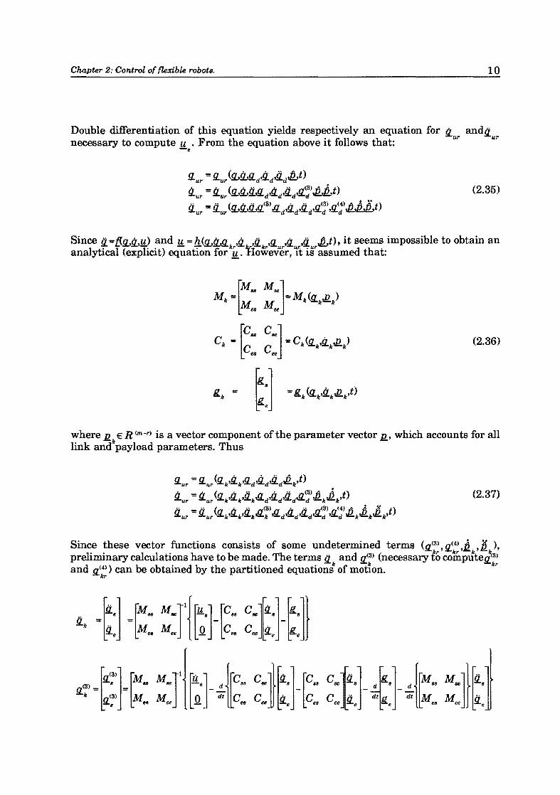
Double differentiation of this equation yields respectively an equation for tl and,q necessary to compute u . From the equation above it follows that: ur ur

-e

(2.35)

Since ,q .. tJg"tJ..,y) and y:.. = h(g"tJ..,!l. ,tl ,,q ,!l. ,tl ii. /bt). it seems impossible to obtain an analytical (explicit) equation forku. ~o«;ever, It iar

assumed that:

(2.36)

where l!. E R (m-r) is a vector component of the parameter vector l!., which accounts for all link andkpayload parameters. Thus

(2.37)

Since these vector functions consists of some undetermined terms (!l(S) ,!l.(4) ,b., ,1 ), preliminary calculations have to be made. The terms!1. and !l.(S) (necessary to co~pJted(S) and !l(4» can be obtained by the partitioned equation' of mot~on. kr

kr

Chapter 2: Control of flexible robots. 11

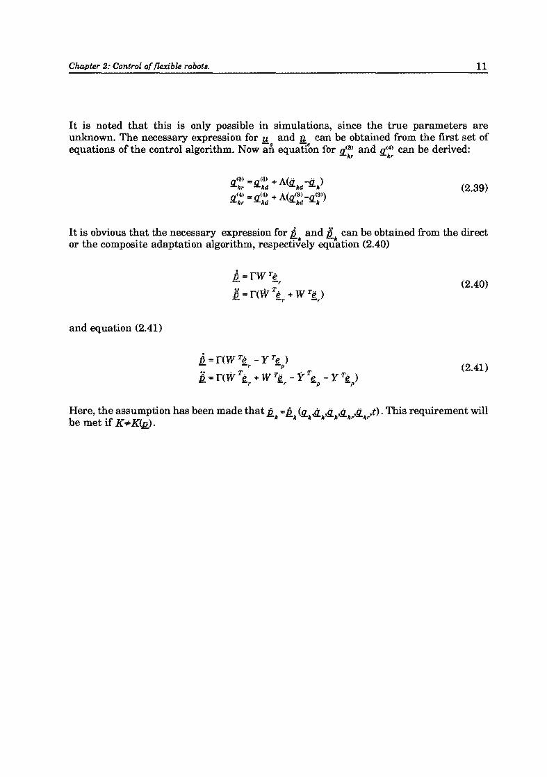
It is noted that this is only possible in simulations, since the true parameters are unknown. The necessary expression for u and it can be obtained from the first set of equations of the control algorithm. Now an equation for ~(S) and q(4) can be derived:

IIr IIr

~(8) '" n(S) + A(ii.. -ii..) IIr ;:;(..lId lid II

n(4) '" ~(4) + A' ,...(8) _~(8» ;:;(..lIr lid '!Llld II

(2.39)

It is obvious that the necessary expression for i and ii. can be obtained from the direct or the composite adaptation algorithm, respecti~ely equ~tion (2.40)

;, ... rwTe J:!.. -r

;:c "" r(W Te + W Te ) J:!... -r -r

(2.40)

and equation (2.41)

(2.41)

Here, the assumption has been made that b.. "" fl ~ .tJ.. ,ii..,{J.. ,ii.. ,0. This requirement will be met if K*K(Ji). II II II k II IIr kr

Chapter 3: Simulations. 12

Chapter 3 Simulations

3.1 The RT-robot

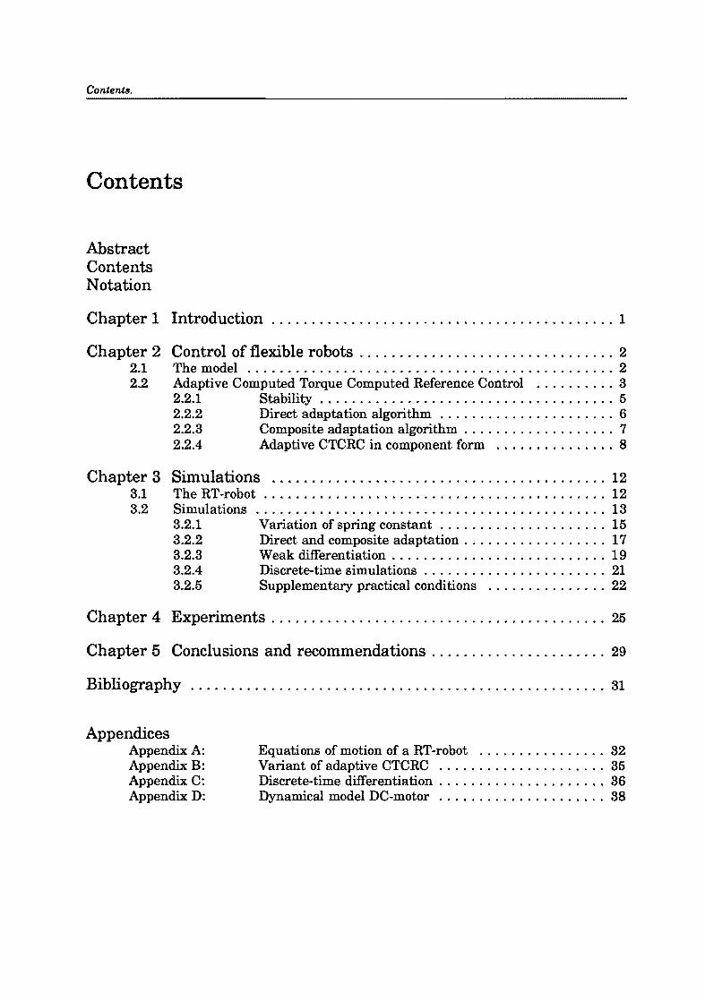
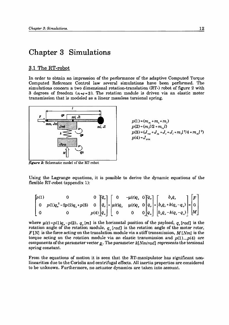
In order to obtain an impression of the performance of the adaptive Computed Torque Computed Reference Control law several simulations have been performed. The simulations concern a two dimensional rotation-translation (RT-) robot of figure 2 with 3 degrees of freedom (n +e -= 3). The rotation module is driven via an elastic motor transmission that is modeled as a linear massless torsional spring.

1

F

figure 2: Schematic model of the RT-robot

p(l)-=(mm +mt+ml )

p(2) '" (m)l2 + mml) p(3) = (Jrot +Jm +Jt +Jl +m tl

2/4 +mml2) p(4)-=JtrTn

Using the Lagrange equations, it is possible to derive the dynamic equations of the flexible RT-robot (appendix 1):

r(1) 0 0 ][iJs

] ~ 0 o p(1)qs2 -2p(2)qs +p(3) 0 iJe + J1(t)qe

o 0 p(4) iJu 0

where J1(t) -=p(l)qs -p(2) , qs [m] is the horizontal position of the payload, q .. [rad] is the rotation angle of the rotation module, q u [rad] is the rotation angle of the motor rotor, F [N] is the force acting on the translation module via a stiff transmission, M [Nm] is the torque acting on the rotation module via an elastic transmission and p(1) ... p(4) are components of the parameter vector ll. The parameter k[Nmlrad] represents the torsional spring constant.

From the equations of motion it is seen that the RT-manipulator has significant non­linearities due to the Coriolis and centrifugal effects. All inertia properties are considered to be unknown. Furthermore, no actuator dynamics are taken into account.

Chapter 3: Simulations. 13

Unless stated otherwise, the following (realistic) parameter values have been chosen:

3 [kg]

3 [Kgm]

I!..... 15 [Kgm 2]

5 [Kgm2] ~8] [1 [N&'m] } Q. "" be = 1 [Nm&'rad]

b 1 [Nm&'radl u

l =2 [m] (3.2) k ",,10[Nm]

The control objective is to let the manipulator track a desired trajectory !l. (t), while keeping all generalized coordinates bounded. The desired trajectory itselfmust~e chosen smooth enough not to excite high frequency dynamics. The desired trajectory for simulation purpose is:

(3.3)

3.2 Simulations

In this paragraph an overview is given of the numerical simulation results. In order to avoid large computation times, it is noted that all system parameters with exception of the parameters of M<!ui) and C(Sl..,(l..Ji) are exactly known. This implies that B*BW). Besides the assumption has been made that the full state vector ;[T,.. IQ T tJ.. T] is available, while for the theoretical situation the second and third derivative (respectively !i. and !l.(3)

can be determined exactly from the equations of motion. For this purpose the true parameters I!.. are substituted in the equations of motion. Obviously this method can only be applied during simulations.

Because it is impractical to assume that the initial position of the end effector always correspond to the desired position, several simulations have been performed with large initial position errors. The presence of relatively large initial position errors e T( 0) "" [SA 2A] results in rapidly fluctuating parameter estimations, due to the fact that - II e the system matrices W = W<!l.,tJ..,tJ.. ,!i. ) and Y"" Y<!l.,tJ..,tLt) and the vector t =t + A! consists of large components. This phenomenon is caused by the gradient nature of the adaption algorithm, i.e. too large adaptation gains or reference signals lead to an oscillatory behaviour of b,.(t). Several approaches are available to obtain a smoother behaviour of the parameter vector b,.(t).

Chapter 3: Simulations. 14

The simplest possibility is to drastically decrease r. since Q -rw Te or Q'" r(W T,[r - yT~ ). This however results in a very slow adaptation process when the system reaches iKe sliding surface (e .0). Note that e (t)*O for t-7 00 as a result of the discontinuous character of the simulations! Therefore-it is possible to extract parameter information from the trajectory errors even when t-7 00 • The upper-boundary cJ> with k 1S:cJ> for t-7 00 is a function of the numerical integration tolerance.

r

Another and more effective approach is to decrease the components Ai of the matrix A, since it reduces the vector ~ =,[ + A~ as well as the system matrices W = W~!i.9:. li. ) and y = y~!L.t). as a result of the reduction in control activity. However this results in large tracking errors ~(t) for t-7 00 , since eiS:cJ>/~.

In order to achieve good trajectory tracking combined with a smooth adaptation process A is chosen to be a time-varying diagonal matrix A=A(t). Assume the system is in sliding motion (e =0) for t>t . Then the general solution of e.+ 1 .(t)e.=0 is:

-r - 8 I ~ I

",-t

ei(t) = ei(ts)exp [- f Alt)d.] ,.-t.

(3.4)

"" This equation is stable for all t>ts if ~(t»O. It is asymptotically stable if [Ai(t)dt=O. For simulations with large initial errors function (3.5) has been applied:

A A 2 A(t)=~t -~sin(.2..t) t max 2n: t max

for t s:tmax (3.5)

for t >tmax

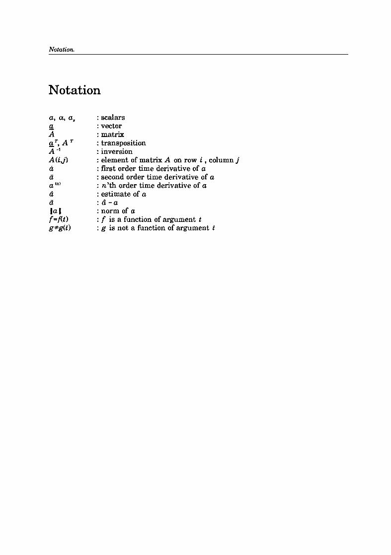
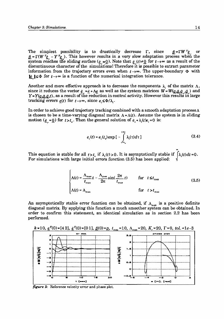
An asymptotically stable error function can be obtained, if ~ax is a positive definite diagonal matrix. By applying this function a much smoother system can be obtained. In order to confirm this statement, an identical simulation as in section 2.2 has been performed.

3

Z

,

i -, ";#' J!: -2

:w -3 .. -e

... '::. ··::::t::::::=:===t::::::::::::::::::r:::::=:::::::::

2.0 r-_---,r--'-p_"' .. _.,._P'-'_Oi:_...,..-_--,

0.15

... __ •••••• 1 •••••••••••••••••• 1. ___ .... .;. ............... . H· .. --···-.. + .. ················t ..•........•.••... l-............ .

=t==t=t.-=. -. 0 HI 20 -0·~'=.---'_':-4--_....I:a=------::!:0--~2 . [ ...... ]. [ ...... ] figure 3: Reference velocity error and phase plot.

Chapter 3: Simulations. 15

3.2.1 Variation of spring constant

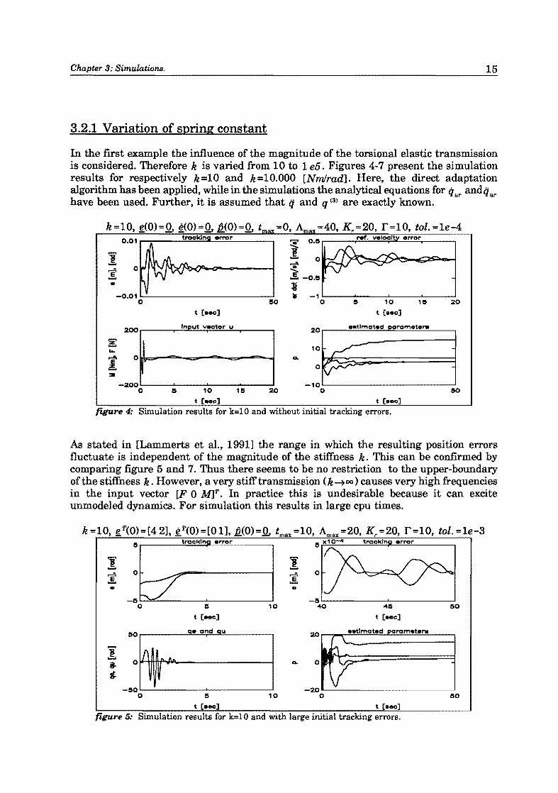
In the fll'St example the influence of the magnitude of the torsional elastic transmission is considered. Therefore k is varied from 10 to 1 e5. Figures 4-7 present the simulation results for respectively k =10 and k =10.000 [NmJrad]. Here, the direct adaptation algorithm has been applied, while in the simulations the analytical equations for q ur and q ur

have been used. Further, it is assumed that q and q (S) are exactly known.

k=10, ~(O)=Q, ~.<o)=Q, Q(O)=Q, t =0, A =40, Kr =20, r=10, tol. =le-4 0.01 traokln error

i 0.15

.......

.! 0 "il' 1a' - -0.15 .. :a

-0.01 • -1 0 150 0 15 10 115 20

t [ •• 0] t [ •• 0]

200 Inl)ut vector u 20 _tlrnot.d rarnet ....

:3 ......

1. 0 v-- Q..

:II

-200 -10 0 15 10 115 20 0 150

t [ •• c] t [8eo]

figure 4: Simulation results for k=10 and without initial tracking errors.

As stated in [Lammerts et al., 1991] the range in which the resulting position errors fluctuate is independent of the magnitude of the stiffness k. This can be confirmed by comparing figure 5 and 7. Thus there seems to be no restriction to the upper-boundary of the stiffness k. However. a very stiff transmission (k -t (X) ) causes very high frequencies in the input vector [F 0 M]T. In practice this is undesirable because it can excite unmodeled dynamics. For simulation this results in large cpu times.

k =10, fT(O) =[4 2], tT(O) =[0 1], Q(O)=Q. tmax =10, Amax =20, Kr =20, r=10, tol. =le-3 15 trackln e,-ror 15 F)(1-=:::0:...-" __ =;.:.:.:.:.:;~:...:.= ___ ..,

50

o 1'1

-150 o

'" A.

~

o

-15~----~----~ 15 10 40 50

t [_]

d ae an au

50

figure 5: Simulation results for k=10 and with large initial tracking errors.

Chapter 3: Simulations. 16

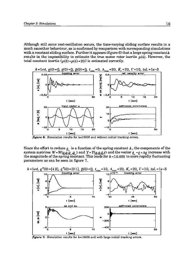
Although still some rest-oscillation occurs, the time-varying sliding surface results in a much smoother behaviour, as is confirmed by comparison with corresponding simulations with a constant sliding surface. Further it appears (figure 6) that a large spring constantk results in the impossibility to estimate the true motor rotor inertia p(4). However, the total constant inertia (p(3) +p(4) =20) is estimated correctly.

! 'S: ........ '"

0.02 ,....-__ ---=t:..:ra:,:c""kI;:..:.n---=e;:..:.rTO.=.r=--__ --, ..... 0.5 ,....-__ ,.:.;I'lIf::.:..!... • ..:.,:vtt::.:;loc=:;:.:.:lt",----=e:.:.,:/TOc..::.:...,r __ --,

ISO

t [aeo]

o

! ....... 'fit 'E' ...... i

o

• -0.15 '-----'-----'----'-----' o 10 11S 20

t [aec]

-20 -10'--------------' o 5 10 15 20 0 50

t [aeo] t [aec]

figure 6: Simulation results for k=lOOOO and without initial tracking errors.

Since the effort to reduce e is a function of the spring constant k, the components of the system matrices W = W(Q,.£~ .ti.. ) and Y = Y(Q,.tJ..,tLt) and the vector! =! + Ag, increase with the magnitude of the spring constant. This leads for k =10.000 to more rapidly fluctuating parameters as can be seen in figure 7.

k=le4, g,T(0)=[42], !T(O)=[Ol], 1l.(0)""Q. tmax ",,10, Amax ",,20, K r =20, r=10, tol.=le-3 10,....-~----=~~~~=------, 10 x10-'" trackln error

I o ~

'" '" -5~------'~----~ o 5 10 45 50

t [aee] t [aee)

200 eetlmated £)Cremet.,..

.. ... 0,

-200

-IS -400'--------------' o 15 10 0 ISO

t [Beo] t [aeo] figure 7: Simulation results for k=lOOOO and with large initial tracking errors.

Chapter 3: Simulations. 17

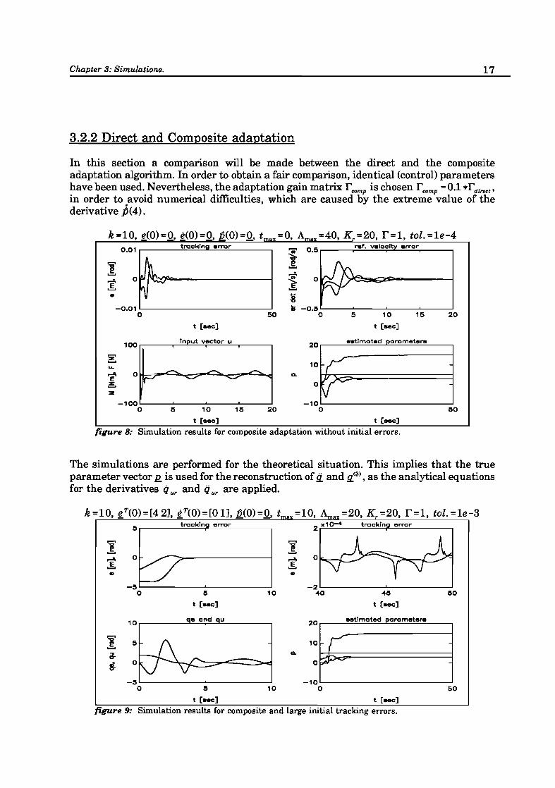
3.2.2 Direct and Composite adaptation

In this section a comparison will be made between the direct and the composite adaptation algorithm. In order to obtain a fair comparison, identical (control) parameters have been used. Nevertheless, the adaptation gain matrix r romp is chosen r romp =0.1 *rdirect'

in order to avoid numerical difficulties, which are caused by the extreme value of the derivative ft(4).

k=10, ~.<o)=Q, ~(O)=Q, Q(O)=Q, t =0, A =40, K =20, r=1, tol. =1e-4 0.01 tr-ackln ern::lr

i 0.5 .... f. veloelt error

! ~

~ ..s .. i -0.01 ~ -0.:5

0 50 0 5 10 15 20

t [sec] t [sec]

100 In ut vector u 20 e.tlmated ramete ....

'Z' ...... ..... ,....1\ 0 a. E .3 :::II!

-100 0 l5 10 115 20 150

t [sec] t [sec]

figure 8: Simulation results for composite adaptation without initial errors.

The simulations are performed for the theoretical situation. This implies that the true parameter vector ll.. is used for the reconstruction of ti.. and !1...(3) , as the analytical equations for the derivatives q ur and q ur are applied.

...... ! ~ ..

...... ! ~ ..

15 10

t [sec]

10r-------~~~~------_,

5 10

2 x10-4

-2L---------~----------~ 40 415 150

t [sec]

20r-__ ~e=.~tim~at=e=d~pa~I~~m~e~t=era~ __ _,

10 r O~ ......

-10~--------------------~ o 50

t [sec] t [sec]

figure 9: Simulation results for composite and large initial tracking errors.

Chapter 3: Simulations. 18

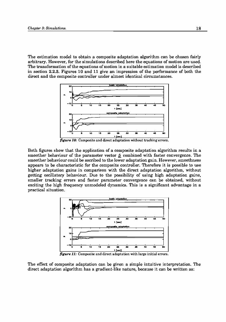
The estimation model to obtain a composite adaptation algorithm can be chosen fairly arbitrary. However, for the simulations described here the equations of motion are used. The transformation of the equations of motion in a suitable estimation model is described in section 2.2.3. Figures 10 and 11 give an impression of the performance of both the direct and the composite controller under almost identical circumstances.

J~§¥: :-~-: : : : J o II 10 III 20 25 30 311 40 4!1 110

t [-l

_~~ . ~-.--. : : : J

o II 10 III 20 21!1 30 311 40 45 110

t ....

figure 10: Composite and direct adaptation without tracking errors.

Both figures show that the application of a composite adaptation algorithm results in a smoother behaviour of the parameter vector b.. combined with faster convergence. The smoother behaviour could be ascribed to the lower adaptation gain. However, smoothness appears to be characteristic for the composite controller. Therefore it is possible to use higher adaptation gains in comparison with the direct adaptation algorithm, without getting oscillatory behaviour. Due to the possibility of using high adaptation gains, smaller tracking errors and faster parameter convergence can be obtained, without exciting the high frequency unmodeled dynamics. This is a significant advantage in a practical situation.

_~re?' .~.-: . . : 1 o II 10 III 20 25 30 311 40 4!1 110

t [-l

_~~ . ~.-' .. : l o II 10 15 20 21!1 30 311 40 411 110

t ....

figure 11: Composite and direct adaptation with large initial errors.

The effect of composite adaptation can be given a simple intuitive interpretation. The direct adaptation algorithm has a gradient-like nature, because it can be written as:

Chapter 3: Simulations. 19

. dHu ii - -'V---==.e

.t::- I dli.-r

This gradient accounts for the poor tracking convergence when a large adaptation gain is used. Since b.. "" Q the composite adaptation law can be written in the following form:

(3.6)

This equation represents a time-varying low pass filter. This means that the parameter errors are now a filtered version of the gradient direction. Thus the parameter search in the composite adaptation goes along a filtered or averaged direction. This indicates that the parameter and tracking error convergence in composite adaptation control can be smoother and faster than in direct control. This conclusion is confirmed by the results represented in the figures above.

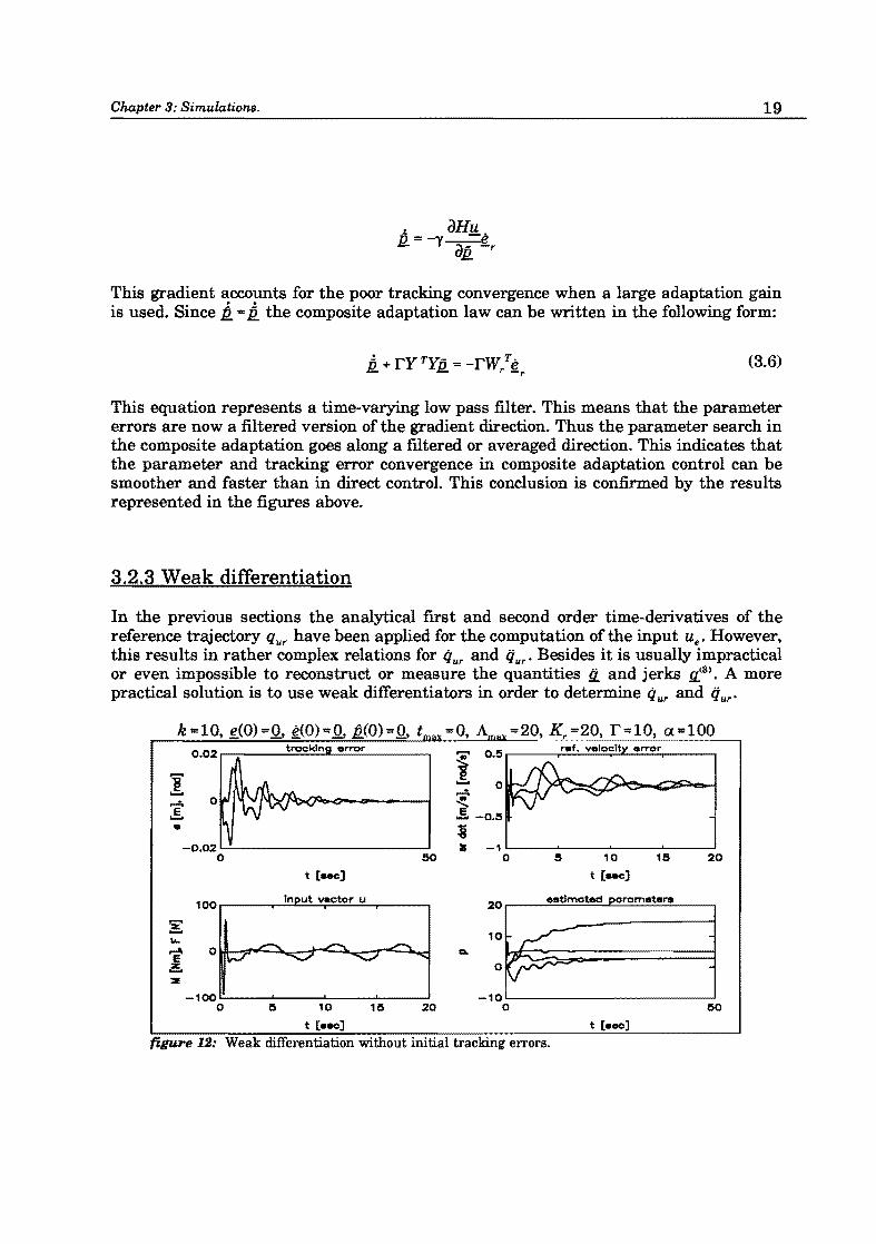
3.2.3 Weak differentiation

In the previous sections the analytical first and second order time-derivatives of the reference trajectory qur have been applied for the computation of the input ue• However, this results in rather complex relations for Qur and tjur' Besides it is usually impractical or even impossible to reconstruct or measure the quantities Ii. and jerks u..(3). A more practical solution is to use weak differentiators in order to determine Q ur and tj ur'

k"'10, !r(0)""Q, g,(0)=Q, 12.(0)=Q, t =0, A =20, K r =20, r=10, t:X=100 0.02 r-: ___ t::..;ro::.;:C;.:.:ki;;..:.na....;;;. .. r;..:..ro;;;.:.r ___ -, ... 0.5,-------,;...::..:..:......:.=.:::.:;:.:.;:.c....;::;;..;..;:;.;;.,.----,

I ...... 0

~ .!. -0.15

i ~ -,~-~--~--~-~

50 0 5 10 15 20

t [INC]

-100~-~--~--~-~ o 15 10 115 20

t [ •• e]

t [INC]

-10L----------------~ o

t [.eel

figure 12: Weak differentiation without initial tracking errors.

Chapter 3: Simulations. ,

Transformation of a first order differentia tor to the Laplace domain yields:

y =:!...u ~ Sf ~ Y(s) = sU(s) = H(s)U(s) dt

If the function H(s) =s is replaced by:

H ·(s) = ~ with a:>O a+s

the following differential equation will be obtained:

ay +y = ail (y -ail) + a(y -au) = -a2u

:i + az = -a2u

20

(3.7)

(3.8)

(3.9)

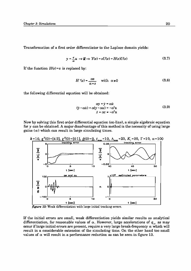
Now by solving this first order differential equation (on-line), a simple algebraic equation for y can be obtained. A major disadvantage of this method is the necessity of using large gains (a) which can result in large simulating times.

k=10, ~T(0)=[42], ~T(O)=[Ol], Q(O)=Q, t =10, =20, Kr=20, r=10, a=100 5 track!" error track;" error

¥ ...... ~

0

• -0.05 '--____ --L-____ ---'

5 10 40 45 50

t [aeel t [.ec]

100 1 x1011 aatlmat.d param.t ....

I 6- ~ O~------------~ ,

-100 -1~---------~ o 5 10 0 50

t [aeel t [eee]

figure 13: Weak differentiation with large initial tracking errors.

If the initial errors are small, weak differentiation yields similar results as analytical differentiation, for reasonable values of a. However, large accelerations of qur as may occur if large initial errors are present, require a very large break-frequency a which will result in a considerable extension of the simulating time. On the other hand too small values of a will result in a performance reduction as can be seen in figure 13.

Chapter 3: Simulations. 21

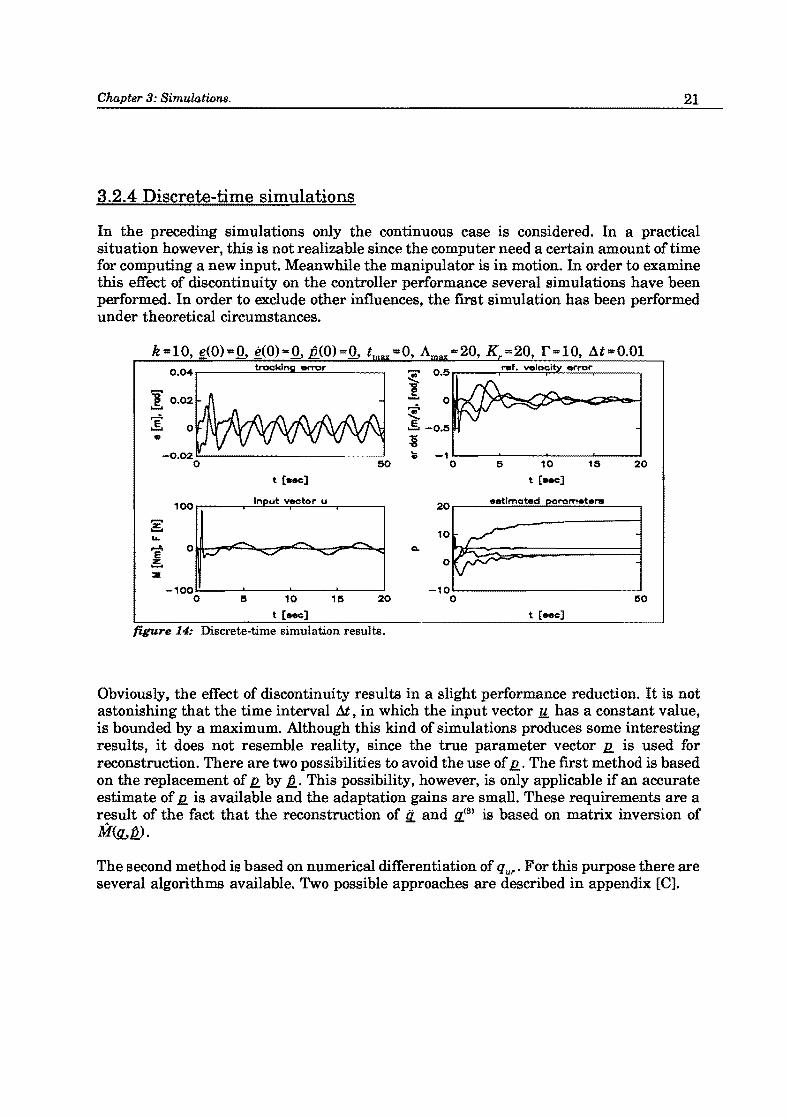
3.2.4 Discrete-time simulations

In the preceding simulations only the continuous case is considered. In a practical situation however, this is not realizable since the computer need a certain amount of time for computing a new input. Meanwhile the manipulator is in motion. In order to examine this effect of discontinuity on the controller performance several simulations have been performed. In order to exclude other influences, the fIrst simulation has been performed under theoretical circumstances.

k=10, ~(O)=Q, e(O)=Q, Q(O)=Q, t =0, A "'20, K =20, r=10, dt=O.01 0.04.--___ t;:;.;I"O=C=ki;;.:."'"---=.elT'O:..:..=I" ___ -.

'f 0.02 ...... ~ • . -,~-~--~--~-~

150 0 15 10 115 20

t [sec] t [..c]

-100~--~--~--~-~ -10~---------~ o 15 115 20 o 150

t [.ee]

figure 14: Discrete-time simulation results.

Obviously, the effect of discontinuity results in a slight performance reduction. It is not astonishing that the time interval M, in which the input vector l! has a constant value, is bounded by a maximum. Although this kind of simulations produces some interesting results, it does not resemble reality. since the true parameter vector Q is used for reconstruction. There are two possibilities to avoid the use of Q. The fIrst method is based on the replacement of Q by IJ... This possibility, however, is only applicable if an accurate estimate of Q is available and the adaptation gains are small. These requirements are a result of the fact that the reconstruction of Ii. and fJ..(S) is based on matrix inversion of M<!LIJ..).

The second method is based on numerical differentiation of q ur' For this purpose there are several algorithms available. Two possible approaches are described in appendix [C].

Chapter 3: Simulations. 22

k ""1000, ~(O) ""Q. ~(O) ""Q. Q(O) ""Q. t ""0, ",,10, K ",,10, r""l, .6.t""O.01 0.1 ...--___ t;;;...f'C=c;.;.;;k·;.;.;.'n.oo......::;e;..;..rt"C= .. ___ __,

i -0.1~---------~ _ -1~-~--~--~-~

o ~ 0 5 10 15 20

t [_eel t [aecl

10...--_~·=~~lm=a=w=d~~rc=m=.=t.=~~ _ __,

-5~---------~ o 50

t [_eel t [Hel

figure 16: Discrete-time and numerical differentiation.

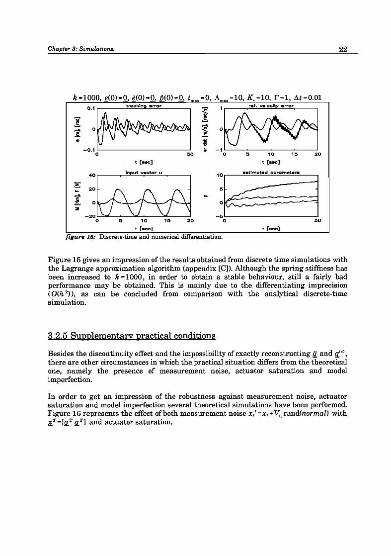
Figure 15 gives an impression of the results obtained from discrete time simulations with the Lagrange approximation algorithm (appendix [CD. Although the spring stiffness has been increased to k ""1000, in order to obtain a stable behaviour, still a fairly bad performance may be obtained. This is mainly due to the differentiating imprecision (O(h 2», as can be concluded from comparison with the analytical discrete-time simulation.

3.2.5 Supplementary practical conditions

Besides the discontinuity effect and the impossibility of exactly reconstructing Ii. and !J..(3) ,

there are other circumstances in which the practical situation differs from the theoretical one, namely the presence of measurement noise, actuator saturation and model imperfection.

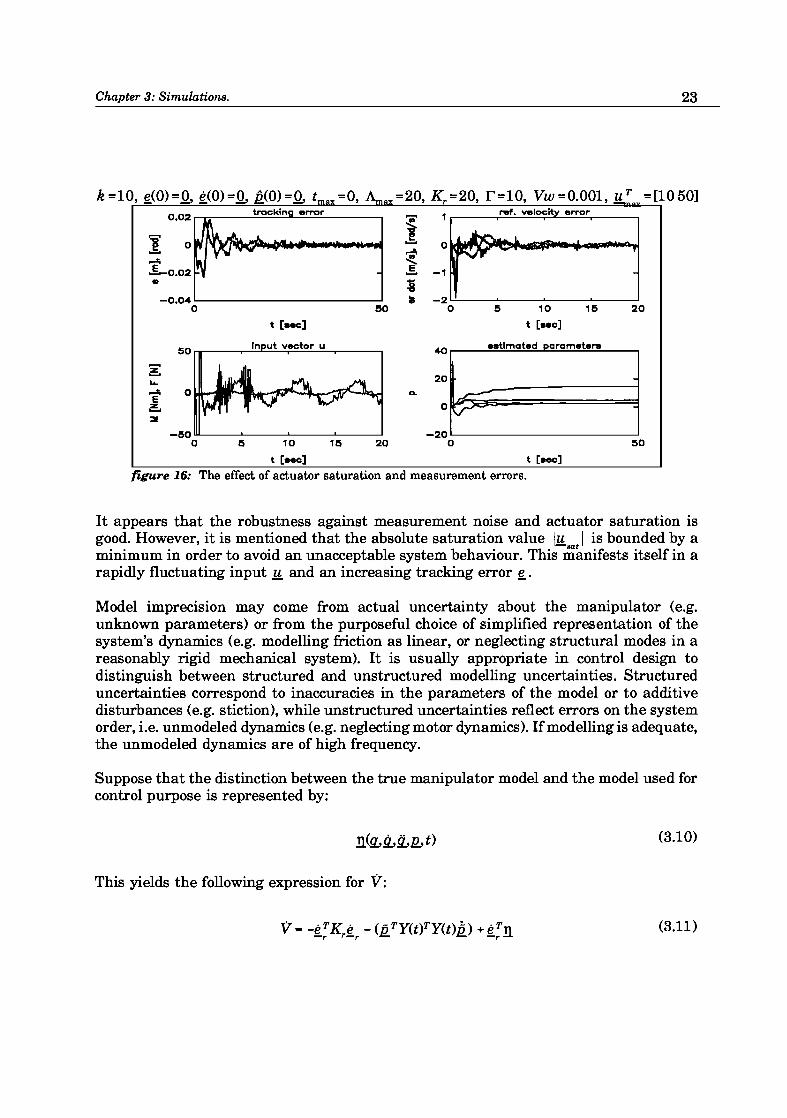
In order to get an impression of the robustness against measurement noise, actuator saturation and model imperfection several theoretical simulations have been performed. Figure 16 represents the effect of both measurement noise X/ ""Xi + Vwrand(normal) with ~T ""lilT QT] and actuator saturation.

Chapter 3: Simulations. 23

k "10, ~(O) .. Q, t(O) .. Q, Q(O) .. Q, t "0, .. 20, K "20, r .. 10, Vw .. O.001, u T "[105O] trackln error

i ref. velocit error

1: ~ 0

t oS -1

• :a -0.04 lis -2

0 50 0 5 10 15 20

t [eec] t [eec]

50 In ut vector u ...a eetlmated parameters

~

~ 20 ....

r4 0 a. ~ E ~ 0 V" :2

-50 -20 0 15 10 115 20 0 150

t [eee] t [eee]

figure 16: The effect of actuator saturation and measurement errors.

It appears that the robustness against measurement noise and actuator saturation is good. However, it is mentioned that the absolute saturation value lu sat I is bounded by a minimum in order to avoid an unacceptable system behaviour. This manifests itself in a rapidly fluctuating input u and an increasing tracking error ~.

Model imprecision may come from actual uncertainty about the manipulator (e.g. unknown parameters) or from the purposeful choice of simplified representation of the system's dynamics (e.g. modelling friction as linear, or neglecting structural modes in a reasonably rigid mechanical system). It is usually appropriate in control design to distinguish between structured and unstructured modelling uncertainties. Structured uncertainties correspond to inaccuracies in the parameters of the model or to additive disturbances (e.g. stiction), while unstructured uncertainties reflect errors on the system order, i.e. unmodeled dynamics (e.g. neglecting motor dynamics). If modelling is adequate, the unmodeled dynamics are of high frequency.

Suppose that the distinction between the true manipulator model and the model used for control purpose is represented by:

(3.10)

This yields the following expression for V:

(3.11)

Chapter 3: Simulations. 24

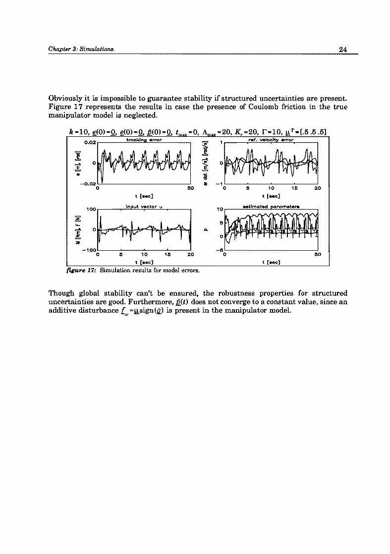
Obviously it is impossible to guarantee stability if structured uncertainties are present. Figure 1 7 represents the results in case the presence of Coulomb friction in the true manipulator model is neglected.

k ... l0, ~(O)""Q, ~'<O)=Q, Q(O)=Q, t -0, =20, K =20, r=10, Mt=[.5.5 .5] 0.02.----___ tt"ac=::;k1:.:..;na....::e :..:..rTO;::.:r ___ ...,

. .... ]: i

-0.02'--'-------------' II -1 '--_--'-__ --'-__ ...1....-_---' 0000 5 20

t [sac]

100r-__ ~~ln~u~t~vTa~ct=o~r~u-r ____ ,

~

i!:.. ..... ~ o~~~~~~~~~~~

i!:..

-100L---~----~----...1....---~ o 10 115 20

t [sec] t [aec]

figure 17: Simulation results for model errors.

Though global stability can't be ensured, the robustness properties for structured uncertainties are good. Furthermore, Q(t) does not converge to a constant value, since an additive disturbance l =1!sign(Q) is present in the manipulator modeL

w

Chapter 4: Experiments. 25

Chapter 4 Experiments

Because the simulations in the previous chapter showed reasonable results, it is worthwhile to test the adaptive CTCRC law under practical circumstances. The practical use of adaptive CTCRC has been verified by means of experiments on a flexible RT­manipulator. This mechanical system isn't deliberately constructed with a torsional transmission. Therefore the spring constant k isn't adjustable and is rather large (k.2 e 1\ [Nmlrad]). Although a large spring constant is in accordance with the reality, it does not clearly express the benefits of a flexible control law. For the experiments the same manipulator model as for the simulations has been used. Obviously this model does not exactly describe the reality, since there are structured uncertainties as well as unmodeled dynamics.

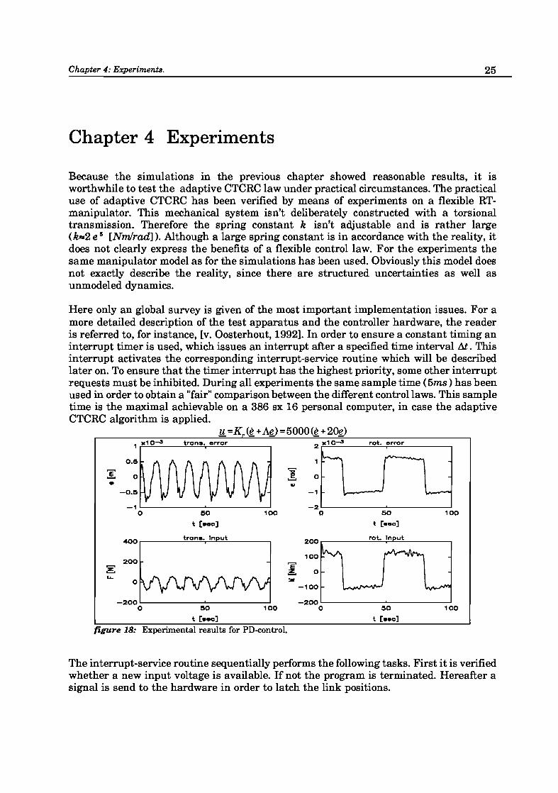
Here only an global survey is given of the most important implementation issues. For a more detailed description of the test apparatus and the controller hardware, the reader is referred to, for instance, [v. Oosterhout, 1992]. In order to ensure a constant timing an interrupt timer is used, which issues an interrupt after a specified time interval !it. This interrupt activates the corresponding interrupt-service routine which will be described later on. To ensure that the timer interrupt has the highest priority, some other interrupt requests must be inhibited. During all experiments the same sample time (5ms) has been used in order to obtain a "fair" comparison between the different control laws. This sample time is the maximal achievable on a 386 sx 16 personal computer, in case the adaptive CTCRC algorithm is applied.

y:. = K (g, + Ag) = 5000 (g, + 2~ 1 x10-.3 t~an". e~~o~

0.5

o

-O.S

50 100

t [ ... c]

400 t~an •• In ut

200 -~ .....

0

-200 0 SO 100

t [ ... c]

figure 18: Experimental results for PD-control.

I :or

2 x10-3

b-'\

o

-1

-2 o

200

100

0

-100

-200 0

.A.

l----

50 100

t [ ... c]

SO

t [ •• c]

The interrupt-service routine sequentially performs the following tasks. First it is verified whether a new input voltage is available. If not the program is terminated. Hereafter a signal is send to the hardware in order to latch the link positions.

Chapter 4: Experiments. 26

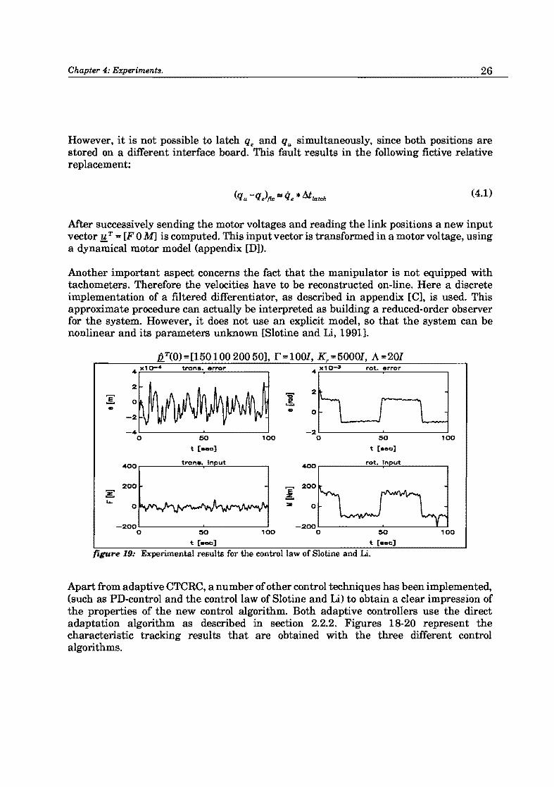
However, it is not possible to latch qe and qu simultaneously, since both positions are stored on a different interface board. This fault results in the following fictive relative replacement:

(4.1)

Mter successively sending the motor voltages and reading the link positions a new input vector!! T "" [F 0 M1 is computed. This input vector is transformed in a motor voltage, using a dynamical motor model (appendix [D]).

Another important aspect concerns the fact that the manipulator is not equipped with tachometers. Therefore the velocities have to be reconstructed on-line. Here a discrete implementation of a fIltered differentiator, as described in appendix [C], is used. This approximate procedure can actually be interpreted as building a reduced-order observer for the system. However, it does not use an explicit model, so that the system can be nonlinear and its parameters unknown [Slotine and Li, 19911.

QT(O) =[150 100 200 50], r=1001, Kr =50001, A =201 trans. error rot. error

I 2

.. o

-2~--------~--------~ 50 100 o 50 100

t [aec] t [ •• e]

400r-____ -=tr=on=.~.~ln==ut~----~ 4OOr-______ r~o~t.~l~n~u~t ______ ~

200

o

-200~--------~--------~ -2oo~--------~------~~ o 50 100 o 50 100

t [sac] t [_.e]

figure 19: Experimental results for the control law of Slotine and Li.

Apart from adaptive CTCRC, a number of other control techniques has been implemented, (such as PD-control and the control law of Slotine and Li) to obtain a clear impression of the properties of the new control algorithm. Both adaptive controllers use the direct adaptation algorithm as described in section 2.2.2. Figures 18-20 represent the characteristic tracking results that are obtained with the three different control algorithms.

Chapter 4: Experiments. 27

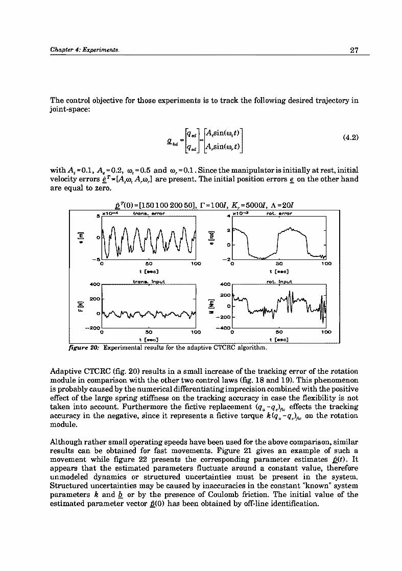
The control objective for those experiments is to track the following desired trajectory in joint-space:

(4.2)

with At ... 0.1, AI! "'0.2, O)t =0.5 and O)r =0.1. Since the manipulator is initially at rest, initial velocity errors ~ T = [AtO)t ArO)r] are present. The initial position errors ~ on the other hand are equal to zero.

~T(0)=[15010020050], r=1001, K =50001, A =201 trons. "lTOr rot. error

I '"

ao 100 50 100

t [s.,e] t [eee]

400r-____ ~tr~Q~n.~.~ln~u~t ____ __, 4OOr-______ I'O==t.,I~n=u=t ______ _,

200

=--200

-200~--------~--------~ -400 ~--------~--------~ o 100 o 80 100

t [eee] t [eee]

figure 20: Experimental results for the adaptive CTCRC algorithm.

Adaptive CTCRC (fig. 20) results in a small increase of the tracking error of the rotation module in comparison with the other two control laws (fig. 18 and 19). This phenomenon is probably caused by the numerical differentiating imprecision combined with the positive effect of the large spring stiffness on the tracking accuracy in case the flexibility is not taken into account. Furthermore the fictive replacement (qu -qe)f!C effects the tracking accuracy in the negative, since it represents a fictive torque k(qu -qe)/ic on the rotation module.

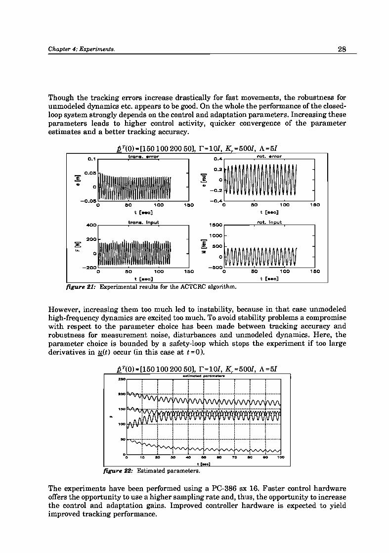
Although rather small operating speeds have been used for the above comparison, similar results can be obtained for fast movements. Figure 21 gives an example of such a movement while figure 22 presents the corresponding parameter estimates ~(t). It appears that the estimated parameters fluctuate around a constant value, therefore unmodeled dynamics or structured uncertainties must be present in the system. Structured uncertainties may be caused by inaccuracies in the constant "known" system parameters k and Q or by the presence of Coulomb friction. The initial value of the estimated parameter vector ~(O) has been obtained by off-line identification.

Chapter 4: Experiments. 28

Though the tracking errors increase drastically for fast movements, the robustness for unmodeled dynamics etc. appears to be good. On the whole the performance of the closed­loop system strongly depends on the control and adaptation parameters. Increasing these parameters leads to higher control activity, quicker convergence of the parameter estimates and a better tracking accuracy.

QT(O) =[150 10020050], r=101, K =5001, A =51 0.1 trans. error 0 ..... rot. e""e"

0.2

:E "Q'

~ 0 G ..

-0.2

-0 ..... SO 100 1S0 0 SO 100 1S0

t [sec] t [sec]

400 1500 rat. In ut

1000 200

I ~ .... =-0

-200 0 150 100 150 50 100 150

t [ •• e] t [ •• e]

figure 21: Experimental results for the ACTCRC algorithm.

However, increasing them too much led to instability, because in that case unmodeled high-frequency dynamics are excited too much. To avoid stability problems a compromise with respect to the parameter choice has been made between tracking accuracy and robustness for measurement noise, disturbances and unmodeled dynamics. Here, the parameter choice is bounded by a safety-loop which stops the experiment if too large derivatives in u(t) occur (in this case at t = 0 ).

QT(O) =[150 100200 50], r=101, K =5001, A=51

o~ __ ~~~~ __ ~ __ ~ __ ~ __ ~ __ ~ __ -L __ ~ o 10 20 30 40 110 110 70 eo 110 100

figure 22: Estimated parameters.

The experiments have been performed using a PC-386 sx 16. Faster control hardware offers the opportunity to use a higher sampling rate and, thus, the opportunity to increase the control and adaptation gains. Improved controller hardware is expected to yield improved tracking performance.

Chapter 5: Conclusions and recommendations.

Chapter 5 Conclusions and recommendations

• From simulations and experiments it appeared that CTCRC is a suitable algorithm for controlling manipulators which are driven via elastic motor transmissions. An important property of the controller is its robustness for unmodeled dynamics, measurement noise and other model imperfections. Furthermore, the magnitude of the spring constant k does not influence the range in between the tracking errors and their time derivatives fluctuate. However, for a rather stiff manipulator unacceptable high frequency signals may occur in the motor inputs.

• To cope with the parametric uncertainty an adaptive version of CTCRC can be applied. Adaptive control is an appealing approach for controlling parameter-uncertain systems. During the simulations two possibilities have been considered, i.e. direct and composite adaptation. The latter not only extracts parameter information from the tracking errors but from the prediction errors as well. The direct adaptation law has a gradient-like nature which accounts for the poor parameter convergence when a large adaptation gain is used. Composite adaptation goes along a filtered, or averaged gradient direction. This indicates that the parameter and tracking error convergence in composite adaptation can be smoother and faster then in direct adaptive control. This smoothness is of great advantage in case unmodeled dynamics are present.

• If the first and the second derivatives of the unknown reference coordinates !1... are derived by numerical differentiation full state availability is required. Use of the analytical derivative also demands the availability of!1...(S) and !1...(4)! For practical implementation full state availability is a necessary and sufficient requirement. If not all state variables are measured a suitable observer must be designed to estimate the unknown deformations and velocities.

• In order to obtain a smooth system behaviour in case large initial position errors are present, a time depending sliding surface has been chosen: e =e+A(t)e -r - -

• The performance of the system strongly depends on an appropriate tuning of the control gains. As a general theory for obtaining control gains is not (yet) available in nonlinear control system design, the simulations are performed with gains obtained by trail and error.

• The transmission flexibility is bounded by a minimum for adaptive CTCRC to be advantageous. This is mainly due to the differentiation imprecision.

29

Chapter 5: Conclusions and recommendations.

•

•

Since differentiating!1.. is the bottle neck of the algorithm, more attention should be paid to the derivation of precise differentiation schemes.

Another topic for future research, is to compare CTCRC with the input· output feedback linearization approach and the method of singular perturbation.

30

Bibliography,

Bibliography

[1] Brevoord, G. Composite computed torque control of the xy-table with an elastic motor transmission -theoretical analysis, simulations and experiments. M.Sc. thesis. Eindhoven, the Netherlands, report WFW 92-054, june 1992.

[2] Doelman, R. Adaptive control of a flexible TR-robot. M.Sc thesis. Eindhoven, the Netherlands, report WFW 92-084, august 1992.

[3] Goode, S. An introduction to differential equations and linear algebra. Prentice Hall, Englewood Cliffs, New Jersey, 1991.

[4] Lammerts, LM.M., F .E. Veldpaus and J.J. Kok. Composite computed torque control of robots with elastic motor transmissions. Proc. of IF ACIIFIPIIMACS Symp. on Robot Control, Vienna, Austria, pp. 193-197, sept 1991.

[5] Lammerts, I.M.M. Adaptive computed reference computed torque control of flexible manipulators. Ph.D. thesis, Eindhoven University of Technology, Dep. of Mechanical Engineering, Eindhoven, the Netherlands, sept 1993.

[6] Mulders, P.C. Besturingstechnologie (in Dutch). Lecture Notes 4603, Eindhoven University of Technology, Dep. of Mechanical Engineer­ing, Eindhoven, the Netherlands, 1991.

[7] Oosterhout van, J.-J. Real time trajectory control of a RT-robot on a single processor computer platform. Mc.S. thesis. Eindhoven, the Netherlands, report WPA-1289, may 1992.

[8] Slotine, J.-J.E. and Li, W. On the adaptive control of robot manipulators. Proc. ASME Winter Annual Meeting, Anaheim, CA., dec. 1986 Int. J. of Robotics Research, vol 6, no.3, pp 49-59, Fall 1987.

[9] Slotine, J.-J.E. and Li, W. Applied nonlinear control. Prentice-Hall, Englewood Cliffs, New Jersey, USA, 1991.

[10] Utkin, V.I. Sliding modes and their applications in variable structure systems. MIR Publishers, Moscow, 1978.

31

Appendices 32

Appendix A: Equations of motion of aRT-robot.

With the Lagrange formalism it is possible to derive the equations of motion. The Lagrange equations are:

(AI)

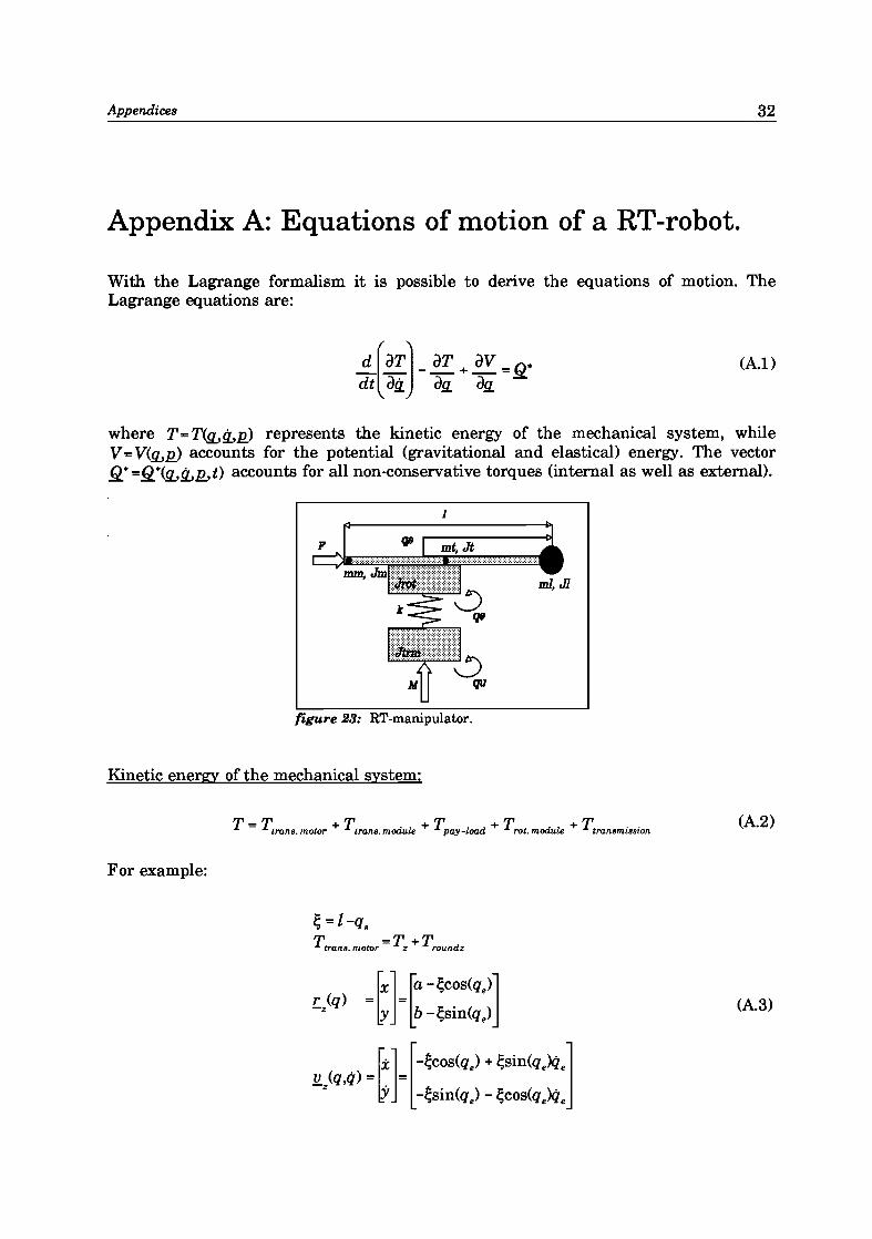
where T=TCsJ..,!i..]2) represents the kinetic energy of the mechanical system, while V = VCsJ..,]2) accounts for the potential (gravitational and elastical) energy. The vector fl.: =fl.:CsJ..,!i..J2..,t) accounts for all non-conservative torques (internal as well as external).

I

11

figure 23: RT-manipulator.

Kinetic energy of the mechanical system:

T = T tran8. motor + T tran8. module + Tpay -load + T rot. module + Ttran8mi88ion (A2)

For example:

~ = l-q8

T tran8. motor = T z + T roundz

(A3)

. [x] [-~cos(q e) + ~sin(q e)q e] V (q,q) = = -z y -~sin(q e) - ~COS(q e)q e

Appendices 33

(A3)

T !:.J . 2 1 {. 2 ( 1)2· 2} trans. motor = 2 mq e +?m q s + q B - q e

(A4)

The kinetic energy is a homogeneous quadratic functon of the generalized velocities tJ... and can be written as:

where: a=(mm +mt +ml )

J3 = (ml/2 +mml)

a

o

o

o

'Y = (J rot +J m +Jt +Jl + m) 2/4 + mm12)

o (A5)

This symmetric inertia matrix M is positive definite because the kinetic energy is strictly positive unless the manipulator is at rest. It is noted that M may not explicitly depend on time t , since in that case the Lagrange ~~malism in the form as stated here cannot be used. With C =!...M + 2.( G - G T) and g. = ~ an expression for the C matrix can be obtained [Lammerfs, 1993]: I a!l..;

-2(aqs - J3~e 01 2(aqs-J3)Qs 0

o 0

This C matrix meets the requirement that (C -!...M) is a skew-symmetric matrix. 2

Potential energy of the mechanical system:

(A6)

The potential energy V for a rigid manipulator with flexible joints consists of a contribution V l due to the deformation of the joints plus a contribution V due to the e cons

Appendices 34

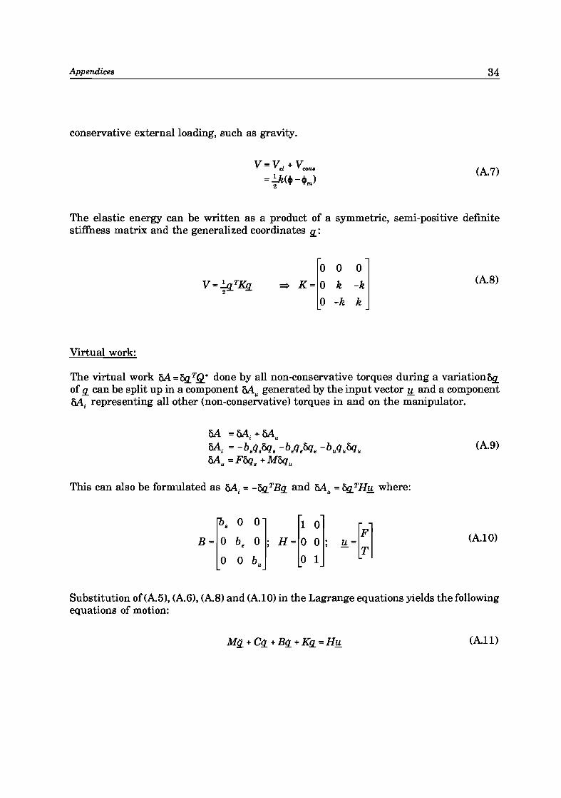
conservative external loading, such as gravity.

v = Vel + Vean•

=¥(cj)-cj)m) (A.7)

The elastic energy can be written as a product of a symmetric, semi-positive definite stiffness matrix and the generalized coordinates !l.:

(A.8)

Virtual work:

The virtual work M =6!J..TQ* done by all non-conservative torques during a variation6!J.. of!l. can be split up in a component Mu generated by the input vector u and a component Mi representing all other (non-conservative) torques in and on the manipulator.

M =Mi+Mu Mi = -b/I.'6q. -b/le'6qe -bllu'6qu Mu =F'6q. +M'6qu

This can also be formulated as Mi = -6!J.. TB!i.. and Mu = 6!J.. THu where:

(A.9)

(A.lO)

Substitution of(A.5), (A.6), (A.8) and (A.lO) in the Lagrange equations yields the following equations of motion:

(A.ll)

Appendices 35

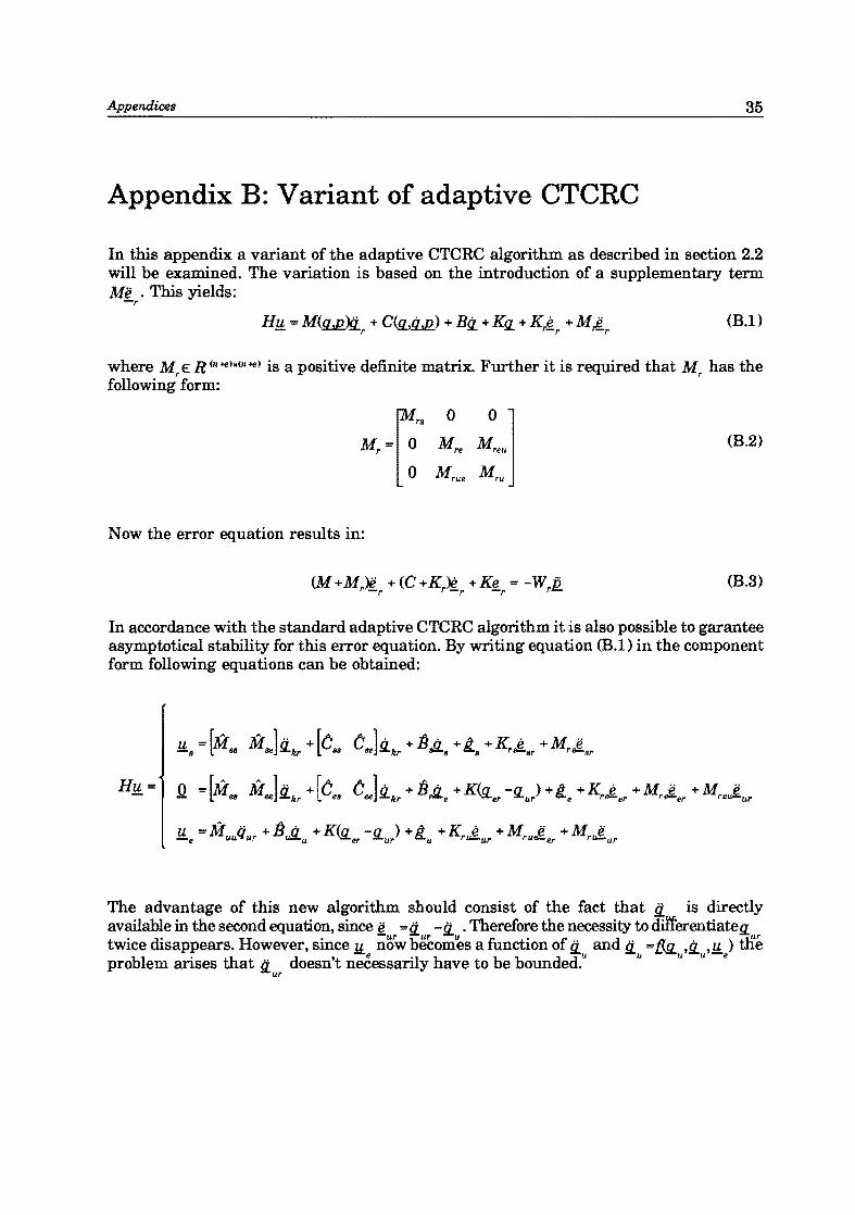
Appendix B: Variant of adaptive CTCRC

In this appendix a variant of the adaptive CTCRC algorithm as described in section 2.2 will be examined. The variation is based on the introduction of a supplementary term Me . This yields:

-r

(B.l)

where Mr E R (n<e)x(n<e) is a positive definite matrix. Further it is required that Mr has the following form:

(B.2)

N ow the error equation results in:

(B.3)

In accordance with the standard adaptive CTCRC algorithm it is also possible to garantee asymptotica1 stability for this error equation. By writing equation (B.l) in the component form following equations can be obtained:

u =[if if]n +[C C]/r <En +b.. +K e +M e -8 88 Be :4..kr 88 Be :4..kr B'LB 8 rs;;;;..Br rs;;;;..sr

o =rif if]n +[c C]n +Bn +K(" -fJ... )+A +K e +M e +M e - l es ee ::L.kr es ee ::L.kr ~e ~er ur 5.e re--er re--er re~ur

The advantage of this new algorithm should consist of the fact that ti.. is directly available in the second equation, since if =ti.. -ti... Therefore the necessity to dtlferentiatefJ...

. di H . ur bur u fi . f d,ff,.. l!'r tWIce sappears. owever, smce u now ecomes a unctIOn 0 ti.. an ti.. = L'Y.. ,tL ,u ) tHe problem arises that ti.. doesn't necessarily have to be bounded.u

u u u-e ur

Appendices 36

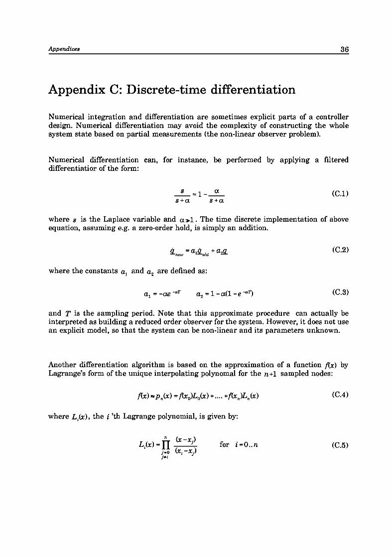
Appendix C: Discrete-time differentiation

Numerical integration and differentiation are sometimes explicit parts of a controller design. Numerical differentiation may avoid the complexity of constructing the whole system state based on partial measurements (the non-linear observer problem).

Numerical differentiation can, for instance, be performed by applying a filtered differentiatior of the form:

_s_:::l_~ (C.l) s+a s+a

where s is the Laplace variable and a>l. The time discrete implementation of above equation, assuming e.g. a zero-order hold, is simply an addition.

;., - a;" + a-n ::L. new - l::L.old :!.:L

where the constants a 1 and a2 are defined as:

a ::: -ae -aT 1

a2

::: l-a(1-e -aT)

(C.2)

(C.3)

and T is the sampling period. Note that this approximate procedure can actually be interpreted as building a reduced order observer for the system. However, it does not use an explicit model, so that the system can be non-linear and its parameters unknown.

Another differentiation algorithm is based on the approximation of a function ({x) by Lagrange's form of the unique interpolating polynomal for the n+l sampled nodes:

(CA)

where L.(x), the i 'th Lagrange polynomial, is given by: •

for i:::O .. n (C.5)

Appendices 37

By differentiating the Lagrange polynomial k times an approximate for the k'th deriva­tive can be obtained:

(C.6)

For any given n+l sampled nodes xi' the above (n+l )-point approximation formula has exactness degree at least n. The guaranteed exactness when fix) is a polynomial of degree ~n follows immediately from the fact that Pn(x) must equal fix) in this case. Formula (C.6) is very general and can be used whether or not the Xi'S are equispaced, and whether or not z is a sampled node Xi'

In case the sampled nodes are equispaced, following O(h 2) backward difference formula in which /j=f(z +jh) can be obtained.

(C.7)

Appendices 38

Appendix D: Dynamical model DC-motor

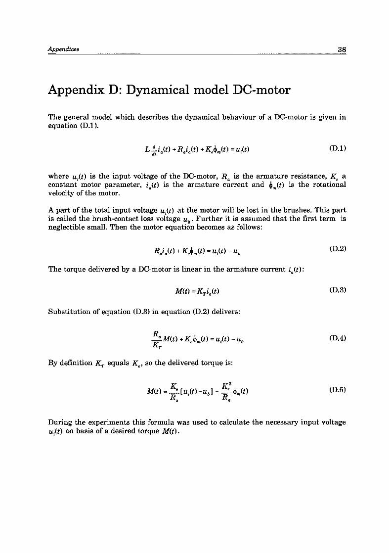
The general model which describes the dynamical behaviour of a DC-motor is given in equation (D.l).

(D.l)

where ut(t) is the input voltage of the DC-motor, Ra is the armature resistance, Ke a constant motor parameter, ia(t) is the armature current and ~m(t) is the rotational velocity of the motor.

A part of the total input voltage ut(t) at the motor will be lost in the brushes. This part is called the brush-contact loss voltage ub • Further it is assumed that the first term is neg1ectib1e small. Then the motor equation becomes as follows:

(D.2)

The torque delivered by a DC-motor is linear in the armature current ia(t):

(D.3)

Substitution of equation (D.3) in equation (D.2) delivers:

(D.4)

By definition KT equals Ke , so the delivered torque is:

(D.5)

During the experiments this formula was used to calculate the necessary input voltage ui(t) on basis of a desired torque M(t).