A M E R I C A N M E T E O R O L O G I C A L S O C I E T Y J A N UA RY 2 0 2 1 E61

Scientific and Human Errors in a Snow Model IntercomparisonCecile B. Menard, Richard Essery, Gerhard Krinner, Gabriele Arduini, Paul Bartlett, Aaron Boone, Claire Brutel-Vuilmet, Eleanor Burke, Matthias Cuntz, Yongjiu Dai, Bertrand Decharme, Emanuel Dutra, Xing Fang, Charles Fierz, Yeugeniy Gusev, Stefan Hagemann, Vanessa Haverd, Hyungjun Kim, Matthieu Lafaysse, Thomas Marke, Olga Nasonova, Tomoko Nitta, Masashi Niwano, John Pomeroy, Gerd Schädler, Vladimir A. Semenov, Tatiana Smirnova, Ulrich Strasser, Sean Swenson, Dmitry Turkov, Nander Wever, and Hua Yuan

ABSTRACT: Twenty-seven models participated in the Earth System Model–Snow Model Inter-comparison Project (ESM-SnowMIP), the most data-rich MIP dedicated to snow modeling. Our findings do not support the hypothesis advanced by previous snow MIPs: evaluating models against more variables and providing evaluation datasets extended temporally and spatially does not facilitate identification of key new processes requiring improvement to model snow mass and energy budgets, even at point scales. In fact, the same modeling issues identified by previous snow MIPs arose: albedo is a major source of uncertainty, surface exchange parameterizations are problematic, and individual model performance is inconsistent. This lack of progress is at-tributed partly to the large number of human errors that led to anomalous model behavior and to numerous resubmissions. It is unclear how widespread such errors are in our field and others; dedicated time and resources will be needed to tackle this issue to prevent highly sophisticated models and their research outputs from being vulnerable because of avoidable human mistakes. The design of and the data available to successive snow MIPs were also questioned. Evaluation of models against bulk snow properties was found to be sufficient for some but inappropriate for more complex snow models whose skills at simulating internal snow properties remained untested. Discussions between the authors of this paper on the purpose of MIPs revealed varied, and sometimes contradictory, motivations behind their participation. These findings started a collaborative effort to adapt future snow MIPs to respond to the diverse needs of the community.

KEYWORDS: Snow; Snowpack; Model comparison; Model evaluation/performance

https://doi.org/10.1175/BAMS-D-19-0329.1Corresponding author: Cecile B. Menard, cmenard@ed.ac.uk Supplemental material: https://doi.org/10.1175/BAMS-D-19-0329.2 In final form 19 August 2020©2020 American Meteorological SocietyFor information regarding reuse of this content and general copyright information, consult the AMS Copyright Policy.

Article

Unauthenticated | Downloaded 01/04/22 01:28 PM UTC

A M E R I C A N M E T E O R O L O G I C A L S O C I E T Y J A N UA RY 2 0 2 1 E62

AFFILIATIONS: Menard and Essery—School of Geosciences, University of Edinburgh, Edinburgh, United

Kingdom; Krinner and Brutel-Vuilmet—Institut de Géosciences de l—Environnement, Université

Grenoble Alpes, CNRS, Grenoble, France; Arduini—European Centre for Medium-Range Weather Forecasts,

Reading, United Kingdom; Bartlett and Decharme—Climate Research Division, Environment and Climate

Change Canada, Toronto, Ontario, Canada; Boone—CNRM, Université de Toulouse, Météo-France, CNRS,

Toulouse, France; Burke—Met Office Hadley Centre, Exeter, United Kingdom; Cuntz—Université de

Lorraine, AgroParisTech, INRAE, UMR Silva, Nancy, France; Dai and Yuan—School of Atmospheric Sciences,

Sun Yat-sen University, Guangzhou, China; Dutra—Instituto Dom Luiz, Faculdade de Ciências, Universi-

dade de Lisboa, Lisbon, Portugal; Fang and Pomeroy—Centre for Hydrology, University of Saskatchewan,

Saskatoon, Saskatchewan, Canada; Fierz—WSL Institute for Snow and Avalanche Research SLF, Davos,

Switzerland; Gusev and Nasonova—Institute of Water Problems, Russian Academy of Sciences, Moscow,

Russia; Hagemann—Institut für Küstenforschung, Helmholtz-Zentrum Geesthacht, Geesthacht, Germany;

Haverd—CSIRO Oceans and Atmosphere, Canberra, Australian Capital Territory, Australia; Kim and Nitta—

Institute of Industrial Science, The University of Tokyo, Tokyo, Japan; Lafaysse—Grenoble Alpes, Université

de Toulouse, Météo-France, CNRS, CNRM, Centre d—Etudes de la Neige, Grenoble, France; Marke and

Strasser—Department of Geography, University of Innsbruck, Innsbruck, Austria; Niwano—Meteorologi-

cal Research Institute, Japan Meteorological Agency, Tsukuba, Japan; Schädler—Institute of Meteorology

and Climate Research, Karlsruhe Institute of Technology, Karlsruhe, Germany; Semenov—A.M. Obukhov

Institute of Atmospheric Physics, Russian Academy of Sciences, Moscow, Russia; Smirnova—Cooperative

Institute for Research in Environmental Science, and NOAA/Earth System Research Laboratory, Boulder,

Colorado; Swenson—Advanced Study Program, National Center for Atmospheric Research, Boulder,

Colorado; Turkov—Institute of Geography, Russian Academy of Sciences, Moscow, Russia; Wever—

Department of Atmospheric and Oceanic Sciences, University of Colorado Boulder, Boulder, Colorado,

and WSL Institute for Snow and Avalanche Research SLF, Davos, Switzerland

The Earth System Model–Snow Model Intercomparison Project (ESM-SnowMIP; Krinner et al. 2018) is the third in a series of MIPs spanning 17 years investigating the performance of snow models. It is closely aligned with the Land Surface, Snow and

Soil Moisture Model Intercomparison Project (LS3MIP; van den Hurk et al. 2016), which is a contribution to the phase 6 of the Coupled Model Intercomparison Project (CMIP6). The Tier 1 reference site simulations (Ref-Site in Krinner et al. 2018), the results of which are discussed in this paper, is the first of 10 planned ESM-SnowMIP experiments and the latest iteration of MIPs using in situ data for snow model evaluation. The Project for Intercomparison of Land Surface Parameterization Schemes Phase 2(d) [PILPS 2(d)] was the first comprehensive intercomparison focusing on the representation of snow in land surface schemes (Pitman and Henderson-Sellers 1998; Slater et al. 2001) and evaluated models at one open site for 18 years. It was followed by the first SnowMIP (hereafter SnowMIP1; Etchevers et al. 2002, 2004), which evaluated models at four open sites for a total of 19 site years, and by SnowMIP2 (Rutter et al. 2009; Essery et al. 2009), which investigated simulations at five open and forested site pairs for nine site years.

Twenty-seven models from 22 modeling teams participated in the ESM-SnowMIP Ref-Site experiment (ESM-SnowMIP hereafter). A short history of critical findings in previous MIPs is necessary to contextualize the results. PILPS 2(d) identified sources of model scatter to be albedo and fractional snow-cover parameterizations controlling the energy available for melt, and longwave radiative feedbacks controlled by exchange coefficients for sensible and latent heat fluxes in stable conditions (Slater et al. 2001). SnowMIP1 corroborated the latter finding, adding that the more complex models were better able to simulate net longwave radiation, but both complex models and simple models with appropriate parameterizations were able

Unauthenticated | Downloaded 01/04/22 01:28 PM UTC

A M E R I C A N M E T E O R O L O G I C A L S O C I E T Y J A N UA RY 2 0 2 1 E63

to simulate albedo well (Etchevers et al. 2004). [Baartman et al. (2020) showed that there is no general consensus about what “model complexity” is; for clarity, we will define models explicitly incorporating larger numbers of processes, interactions, and feedbacks as more complex.] SnowMIP2 found little consistency in model performance between years or sites and, as a result, there was no subset of better models (Rutter et al. 2009). The largest errors in mass and energy balances were attributed to uncertainties in site-specific parameter se-lection rather than to model structure. All these projects concluded that more temporal and spatial data would improve our understanding of snow models and reduce the uncertainty associated with process representations and feedbacks on the climate.

This paper discusses results from model simulations at five mountain sites (Col de Porte, France; Reynolds Mountain East, Idaho, United States; Senator Beck and Swamp Angel, Colorado, United States; Weissfluhjoch, Switzerland), one urban maritime site (Sapporo, Japan), and one Arctic site (Sodankylä, Finland); results for three forested sites will be dis-cussed in a separate publication. Details of the sites, and of forcing and evaluation data are presented in Ménard et al. (2019). Although the 97 site-years of data for these seven reference sites may still be insufficient, they do respond to the demands of previous MIPs by providing more sites in different snowy environments over more years.

The false hypothesisIn fiction, a false protagonist is one who is presented as the main character but turns out not to be, often by being killed off early [e.g., Marion Crane in Psycho (Hitchcock 1960), Dallas in Alien (Scott 1979), Ned Stark in A Game of Thrones (Martin 1996)]. This narrative tech-nique is not used in scientific literature, even though many scientific hypotheses advanced in project proposals are killed early at the research stage. Most scientific journals impose strict manuscript composition guidelines to encourage research studies to be presented in a linear and cohesive manner. As a consequence, many “killed” hypotheses are never presented, and neither are the intermediary steps that lead to the final hypothesis. This is an artifice that we all comply with even though “hypothesizing after the results are known” (known as HARKing; Kerr 1998) is a practice associated with the reproduction crisis (Munafò et al. 2017).

Our working hypothesis was formed at the design stage of ESM-SnowMIP and is explicit in Krinner et al. (2018): more sites over more years will help us to identify crucial processes and characteristics that need to be improved as well as previously unrecognized weaknesses in snow models. However, months of analyzing results led us to conclude the unexpected: more sites, more years, and more variables do not provide more insight into key snow processes. Instead, this leads to the same conclusions as previous MIPs: albedo is still a major source of uncertainty, surface exchange parameterizations are still problematic, and individual model performance is inconsistent. In fact, models are less classifiable with results from more sites, years and evaluation variables. Our initial, or false, hypothesis had to be killed off.

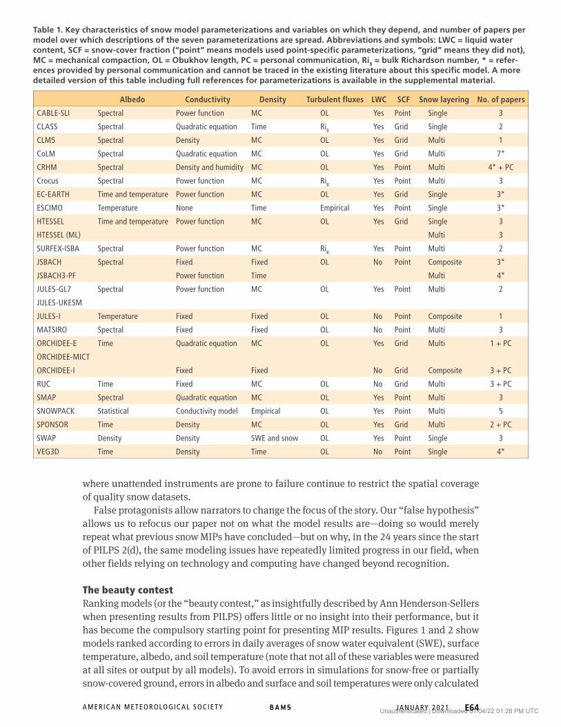
Developments have been made, particularly in terms of the complexity of snow process rep-resentations, and conclusions from PILPS2(d) and snow MIPs have undoubtedly driven model development. Table 1 shows that few participating models now have a fixed snow density or thermal conductivity, only two models still parameterize snow albedo as a simple function of temperature, no model uses constant surface exchange coefficients, more models can now represent liquid water in snow, and only three still have a composite snow–soil layer. These changes demonstrate progress for individual models, but they do not for snow science: most of these parameterizations have existed for decades. Differences between models remain, but the range of model complexity is smaller than it was in previous MIPs.

The pace of advances in snow modeling and other fields in climate research is limited by the time it takes to collect long-term datasets and to develop methods for measuring complex processes. Furthermore, the logistical challenges of collecting reliable data in environments

Unauthenticated | Downloaded 01/04/22 01:28 PM UTC

A M E R I C A N M E T E O R O L O G I C A L S O C I E T Y J A N UA RY 2 0 2 1 E64

where unattended instruments are prone to failure continue to restrict the spatial coverage of quality snow datasets.

False protagonists allow narrators to change the focus of the story. Our “false hypothesis” allows us to refocus our paper not on what the model results are—doing so would merely repeat what previous snow MIPs have concluded—but on why, in the 24 years since the start of PILPS 2(d), the same modeling issues have repeatedly limited progress in our field, when other fields relying on technology and computing have changed beyond recognition.

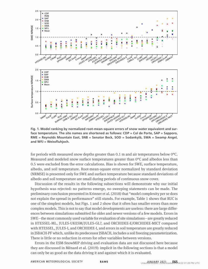
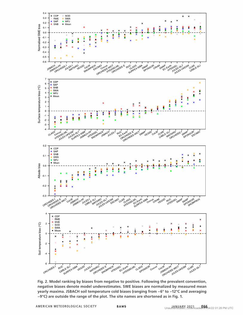
The beauty contestRanking models (or the “beauty contest,” as insightfully described by Ann Henderson-Sellers when presenting results from PILPS) offers little or no insight into their performance, but it has become the compulsory starting point for presenting MIP results. Figures 1 and 2 show models ranked according to errors in daily averages of snow water equivalent (SWE), surface temperature, albedo, and soil temperature (note that not all of these variables were measured at all sites or output by all models). To avoid errors in simulations for snow-free or partially snow-covered ground, errors in albedo and surface and soil temperatures were only calculated

Table 1. Key characteristics of snow model parameterizations and variables on which they depend, and number of papers per model over which descriptions of the seven parameterizations are spread. Abbreviations and symbols: LWC = liquid water content, SCF = snow-cover fraction (“point” means models used point-specific parameterizations, “grid” means they did not), MC = mechanical compaction, OL = Obukhov length, PC = personal communication, RiB = bulk Richardson number, * = refer-ences provided by personal communication and cannot be traced in the existing literature about this specific model. A more detailed version of this table including full references for parameterizations is available in the supplemental material.

Albedo Conductivity Density Turbulent fluxes LWC SCF Snow layering No. of papers

CABLE-SLI Spectral Power function MC OL Yes Point Single 3

CLASS Spectral Quadratic equation Time RiB Yes Grid Single 2

CLM5 Spectral Density MC OL Yes Grid Multi 1

CoLM Spectral Quadratic equation MC OL Yes Grid Multi 7*

CRHM Spectral Density and humidity MC OL Yes Point Multi 4* + PC

Crocus Spectral Power function MC RiB. Yes Point Multi 3

EC-EARTH Time and temperature Power function MC OL Yes Grid Single 3*

ESCIMO Temperature None Time Empirical Yes Point Single 3*

HTESSEL Time and temperature Power function MC OL Yes Grid Single 3

HTESSEL (ML) Multi 3

SURFEX-ISBA Spectral Power function MC RiB. Yes Point Multi 2

JSBACH Spectral Fixed Fixed OL No Point Composite 3*

JSBACH3-PF Power function Time Multi 4*

JULES-GL7 Spectral Power function MC OL Yes Point Multi 2

JULES-UKESM

JULES-I Temperature Fixed Fixed OL No Point Composite 1

MATSIRO Spectral Fixed Fixed OL No Point Multi 3

ORCHIDEE-E Time Quadratic equation MC OL Yes Grid Multi 1 + PC

ORCHIDEE-MICT

ORCHIDEE-I Fixed Fixed No Grid Composite 3 + PC

RUC Time Fixed MC OL No Grid Multi 3 + PC

SMAP Spectral Quadratic equation MC OL Yes Point Multi 3

SNOWPACK Statistical Conductivity model Empirical OL Yes Point Multi 5

SPONSOR Time Density MC OL Yes Grid Multi 2 + PC

SWAP Density Density SWE and snow OL Yes Point Single 3

VEG3D Time Density Time OL No Point Single 4*

Unauthenticated | Downloaded 01/04/22 01:28 PM UTC

A M E R I C A N M E T E O R O L O G I C A L S O C I E T Y J A N UA RY 2 0 2 1 E65

for periods with measured snow depths greater than 0.1 m and air temperatures below 0°C. Measured and modeled snow surface temperatures greater than 0°C and albedos less than 0.5 were excluded from the error calculations. Bias is shown for SWE, surface temperature, albedo, and soil temperature. Root-mean-square error normalized by standard deviation (NRMSE) is presented only for SWE and surface temperature because standard deviations of albedo and soil temperature are small during periods of continuous snow cover.

Discussion of the results in the following subsections will demonstrate why our initial hypothesis was rejected: no patterns emerge, no sweeping statements can be made. The preliminary conclusion presented in Krinner et al. (2018) that “model complexity per se does not explain the spread in performance” still stands. For example, Table 1 shows that RUC is one of the simplest models, but Figs. 1 and 2 show that it often has smaller errors than more complex models. This is not to say that model developments are useless: there are large differ-ences between simulations submitted for older and newer versions of a few models. Errors in SWE—the most commonly used variable for evaluation of site simulations—are greatly reduced in HTESSEL-ML, JULES-UKESM/JULES-GL7, and ORCHIDEE-E/ORCHIDEE-MICT compared with HTESSEL, JULES-I, and ORCHIDEE-I, and errors in soil temperature are greatly reduced in JSBACH-PF which, unlike its predecessor JSBACH, includes a soil freezing parameterization. There is little or no reduction in errors for other variables between versions.

Errors in the ESM-SnowMIP driving and evaluation data are not discussed here because they are discussed in Ménard et al. (2019): implicit in the following sections is that a model can only be as good as the data driving it and against which it is evaluated.

Fig. 1. Model ranking by normalized root-mean-square errors of snow water equivalent and sur-face temperature. The site names are shortened as follows: CDP = Col de Porte, SAP = Sapporo, RME = Reynolds Mountain East, SNB = Senator Beck, SOD = Sodankylä, SWA = Swamp Angel, and WFJ = Weissfluhjoch.

Unauthenticated | Downloaded 01/04/22 01:28 PM UTC

A M E R I C A N M E T E O R O L O G I C A L S O C I E T Y J A N UA RY 2 0 2 1 E66

Fig. 2. Model ranking by biases from negative to positive. Following the prevalent convention, negative biases denote model underestimates. SWE biases are normalized by measured mean yearly maxima. JSBACH soil temperature cold biases (ranging from −6° to −12°C and averaging −9°C) are outside the range of the plot. The site names are shortened as in Fig. 1.

Unauthenticated | Downloaded 01/04/22 01:28 PM UTC

A M E R I C A N M E T E O R O L O G I C A L S O C I E T Y J A N UA RY 2 0 2 1 E67

Snow water equivalent and surface temperature. Mean SWE and surface temperature NRMSEs in Fig. 1 are generally low: below 0.6 for half of the models and 1 or greater for only four models. Biases are also relatively low: less than 2°C in surface temperature and less than 0.2 in normalized SWE for four out of five sites in Fig. 2. The sign of the biases in surface temperature are the same for at least four out of five sites for all except four models (JULES-I, ORCHIDEE-E, ORCHIDEE-MICT, and SWAP). The six models with the largest negative biases in SWE are among the seven models that do not represent liquid water in snow. The seventh model, RUC, has its largest negative bias at Sapporo, where rain-on-snow events are common. Wind-induced snow redistribution, which no model simulates at a point, is partly responsible for Senator Beck being one of the two sites with largest SWE NRMSE in more than half of the models.

Four of the best models for SWE NRMSE are among the worst for surface temperature NRMSE (SPONSOR, Crocus, CLASS, and HTESSEL-ML). Decoupling of the snow surface from the atmosphere under stable conditions is a long-standing issue, which Slater et al. (2001) investigated in PILPS 2(d). Underestimating snow surface temperature leads to a colder snowpack that takes longer to melt and remains on the ground for longer. In 2001, most models used Richardson numbers to calculate surface exchange; in 2019, most use Monin–Obukhov similarity theory (MOST). However, assumptions of flat and horizontally homo-geneous surfaces and steady-state conditions in MOST make it inappropriate for describing conditions not only over snow surfaces, but also over forest clearings and mountains: in other words, at all sites in this study. Exchange coefficient are commonly used to tune near-surface temperature in numerical weather prediction models even if to the detriment of the representation of stable boundary layers (Sandu et al. 2013). Conway et al. (2018) showed that such tuning in snowpack modeling improved surface temperature simula-tions but at the expense of overestimating melt. It is beyond the scope of this paper (and in view of the discussion on sources of errors in the “Discussion” section, possibly beyond individual modeling teams) to assess how individual models have developed and evaluated their surface exchange and snowpack evolution schemes. However, differences in model ranking between SWE and surface temperature suggest that this issue is widespread and warrants further attention.

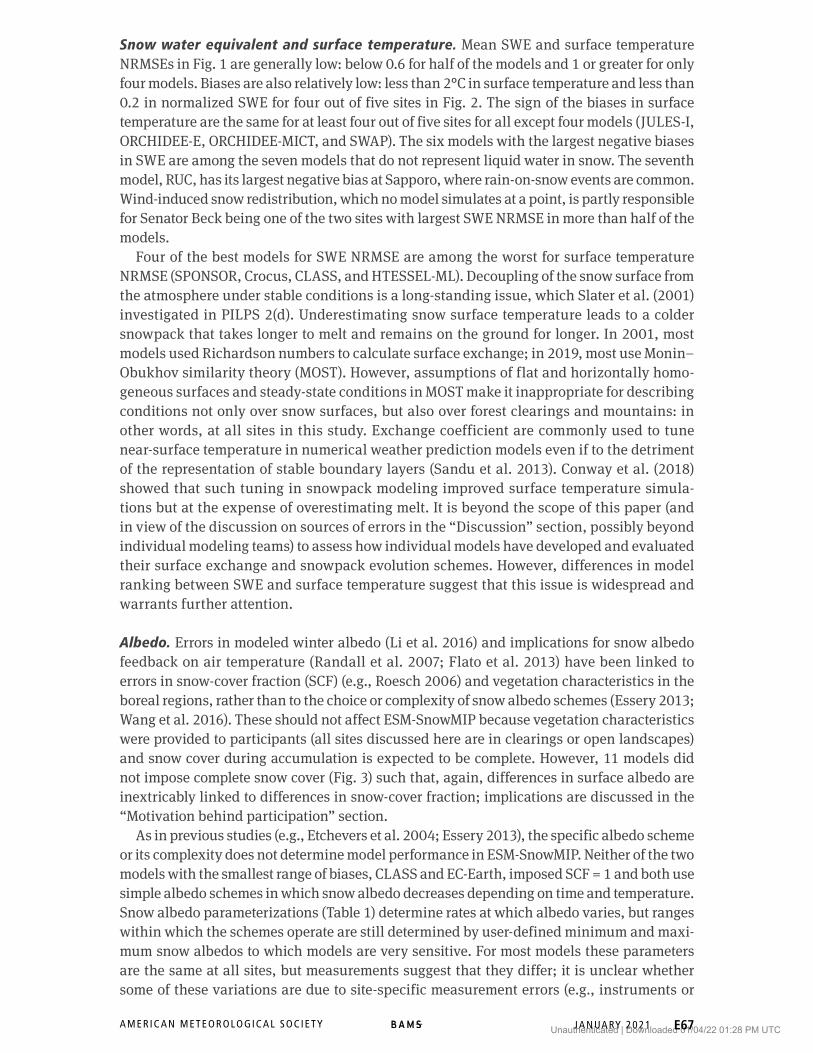
Albedo. Errors in modeled winter albedo (Li et al. 2016) and implications for snow albedo feedback on air temperature (Randall et al. 2007; Flato et al. 2013) have been linked to errors in snow-cover fraction (SCF) (e.g., Roesch 2006) and vegetation characteristics in the boreal regions, rather than to the choice or complexity of snow albedo schemes (Essery 2013; Wang et al. 2016). These should not affect ESM-SnowMIP because vegetation characteristics were provided to participants (all sites discussed here are in clearings or open landscapes) and snow cover during accumulation is expected to be complete. However, 11 models did not impose complete snow cover (Fig. 3) such that, again, differences in surface albedo are inextricably linked to differences in snow-cover fraction; implications are discussed in the “Motivation behind participation” section.

As in previous studies (e.g., Etchevers et al. 2004; Essery 2013), the specific albedo scheme or its complexity does not determine model performance in ESM-SnowMIP. Neither of the two models with the smallest range of biases, CLASS and EC-Earth, imposed SCF = 1 and both use simple albedo schemes in which snow albedo decreases depending on time and temperature. Snow albedo parameterizations (Table 1) determine rates at which albedo varies, but ranges within which the schemes operate are still determined by user-defined minimum and maxi-mum snow albedos to which models are very sensitive. For most models these parameters are the same at all sites, but measurements suggest that they differ; it is unclear whether some of these variations are due to site-specific measurement errors (e.g., instruments or

Unauthenticated | Downloaded 01/04/22 01:28 PM UTC

A M E R I C A N M E T E O R O L O G I C A L S O C I E T Y J A N UA RY 2 0 2 1 E68

vegetation in the radiometer field of view). This issue should be investigated further as this is not the first time that model results have been inconclusive because of such uncertainties (e.g., Essery et al. 2013).

Soil temperature. Five models systematically underestimate soil temperatures under snow (JSBACH, MATSIRO, ORCHIDEE-I, RUC, and SURFEX-ISBA) and four systematically overes-timate them (CLM5, CoLM, JULES-GL7, and ORCHIDEE-MICT), although negative biases are often larger than positive ones. Soil temperatures are not consistently over- or underestimated by all models at any particular site. Three of the models (JSBACH, JULES-I, and ORCHIDEE-I) still include a thermally composite snow–soil layer, and the lack of a soil moisture freezing

Fig. 3. Fractional snow cover (SCF) as a function of SWE at Col de Porte for models that did not switch off their subgrid parameterizations or impose complete snow cover. HTESSEL is not shown as it is the same as HTESSEL-ML. ORCHIDEE-MICT did not force SCF = 1, but values were missing from the file provided for evaluation.

Unauthenticated | Downloaded 01/04/22 01:28 PM UTC

A M E R I C A N M E T E O R O L O G I C A L S O C I E T Y J A N UA RY 2 0 2 1 E69

representation in JSBACH causes soil temperatures to be underestimated. Although newer versions of these models (ORCHIDEE-E, ORCHIDEE-MICT, JSBACH-PF, JULES-GL7, and JULES-UKESM) include more realistic snow–soil process representations, cold biases of the implicit versions have, with the exception of ORCHIDEE-E, been replaced by warm biases, and of similar magnitude between JULES-I and JULES-GL7.

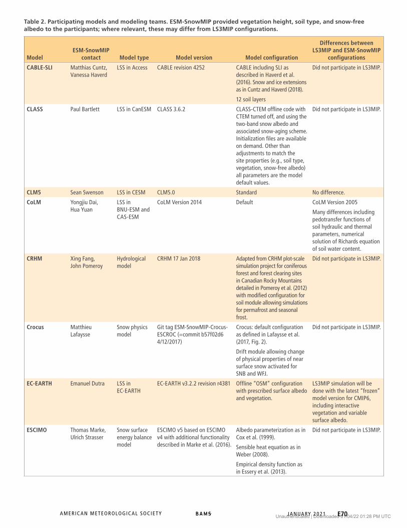
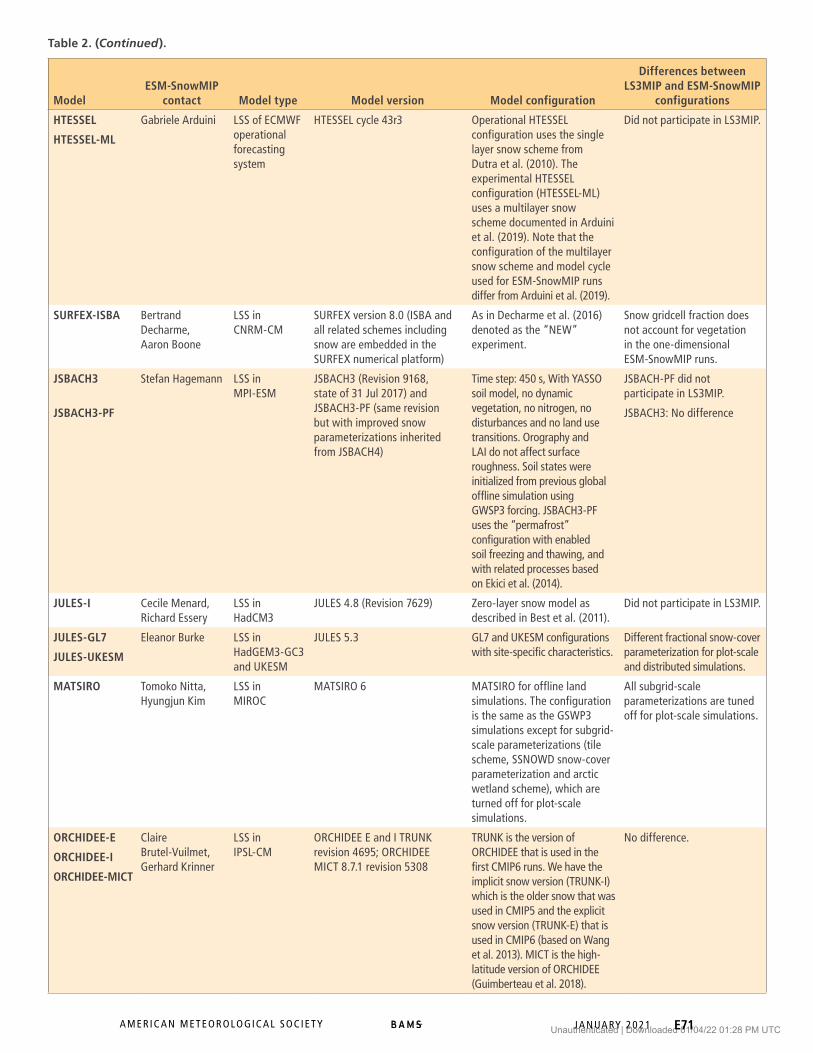
DiscussionMotivation behind participation. One of the motivations behind the design of ESM-SnowMIP was to run a stand-alone MIP dedicated to snow processes parallel to other MIPs, most notably CMIP6 and LS3MIP: “Combining the evaluation of these global-scale simulations with the detailed process-based assessment at the site scale provides an opportunity for substantial progress in the representation of snow, particularly in Earth system models that have not been evaluated in detail with respect to their snow parameterizations” (Krinner et al. 2018). Identifying errors in ESM-SnowMIP site simulations could be linked to model processes that also operate in LS3MIP global simulations, separately from meteorological and ancillary data errors. However, LS3MIP and ESM-SnowMIP results are not directly comparable because land surface schemes (LSSs) include parameterizations that describe subgrid heterogeneity and some LSSs allow them to be switched off or modified for point simulations. Tables 1 and 2 show whether models participated in both MIPs and whether they used point simulation-specific snow-cover parameterizations, which is critical for albedo and the most common parameterization to simulate subgrid heterogeneity. Of the 11 models that did not adjust their subgrid parameterizations or impose complete snow cover (Fig. 3), only one (CLASS) is not participating in LS3MIP. Of those that are participating, three switched off their subgrid parameterizations (MATSIRO, RUC, and SURFEX-ISBA). Had it been anticipated at the design stage that some models would have considered ESM-SnowMIP to be a means to evaluate their LS3MIP setup against in situ data, ESM-SnowMIP instructions would have advised to switch off all subgrid processes; treating a point simulation like a spatial simulation makes evaluating some variables against point measurements futile. This is best illustrated with ORCHIDEE, the three versions of which have the highest negative albedo biases; not only was complete snow cover not imposed, but also the maximum albedo for deep snow on grass (i.e., 0.65 at all sites except Weissfluhjoch) accounts implicitly for subgrid heterogeneity in large-scale simulations.

Although called ESM-SnowMIP, the site simulations were always intended to include physically based snow models that are not part of an ESM but have other applications (Krinner et al. 2018). Table 3 lists what motivated different groups to participate in ESM-SnowMIP. Although not explicit in Table 3 because of the anonymity of the comments, for developers of snow physics models, the motivation to participate in a MIP dedicated to scrutinizing the processes they investigate is self-evident. On the other hand, most land surface schemes were first developed to provide the lower boundary conditions to atmo-spheric models. Because of the dramatic differences in the energy budget of snow-free and snow-covered land, the main requirement for snow models in some LSSs is still just to inform atmospheric models of whether there is snow on the ground or not. The size of the modeling group also matters; more models supported by a single individual or small teams listed exposure as one of their motivations. This discussion revealed that many par-ticipants suffered from the “false consensus effect” (Lee et al. 1977), also observed among geoscientists but not explicitly named by Baartman et al. (2020), i.e., they assumed their motivations were universal, or at the very least, widespread. Ultimately, the prestige of MIPs means that, regardless of workload, personal motivation or model performance, they have become compulsory promotional exercises that we cannot afford not to participate in, for better or worse.

Unauthenticated | Downloaded 01/04/22 01:28 PM UTC

A M E R I C A N M E T E O R O L O G I C A L S O C I E T Y J A N UA RY 2 0 2 1 E70

Table 2. Participating models and modeling teams. ESM-SnowMIP provided vegetation height, soil type, and snow-free albedo to the participants; where relevant, these may differ from LS3MIP configurations.

ModelESM-SnowMIP

contact Model type Model version Model configuration

Differences between LS3MIP and ESM-SnowMIP

configurations

CABLE-SLI Matthias Cuntz, Vanessa Haverd

LSS in Access CABLE revision 4252 CABLE including SLI as described in Haverd et al. (2016). Snow and ice extensions as in Cuntz and Haverd (2018).

Did not participate in LS3MIP.

12 soil layers

CLASS Paul Bartlett LSS in CanESM CLASS 3.6.2 CLASS-CTEM offline code with CTEM turned off, and using the two-band snow albedo and associated snow-aging scheme. Initialization files are available on demand. Other than adjustments to match the site properties (e.g., soil type, vegetation, snow-free albedo) all parameters are the model default values.

Did not participate in LS3MIP.

CLM5 Sean Swenson LSS in CESM CLM5.0 Standard No difference.

CoLM Yongjiu Dai, Hua Yuan

LSS in BNU-ESM and CAS-ESM

CoLM Version 2014 Default CoLM Version 2005

Many differences including pedotransfer functions of soil hydraulic and thermal parameters, numerical solution of Richards equation of soil water content.

CRHM Xing Fang, John Pomeroy

Hydrological model

CRHM 17 Jan 2018 Adapted from CRHM plot-scale simulation project for coniferous forest and forest clearing sites in Canadian Rocky Mountains detailed in Pomeroy et al. (2012) with modified configuration for soil module allowing simulations for permafrost and seasonal frost.

Did not participate in LS3MIP.

Crocus Matthieu Lafaysse

Snow physics model

Git tag ESM-SnowMIP-Crocus- ESCROC (=commit b57f02d6 4/12/2017)

Crocus: default configuration as defined in Lafaysse et al. (2017, Fig. 2).

Did not participate in LS3MIP.

Drift module allowing change of physical properties of near surface snow activated for SNB and WFJ.

EC-EARTH Emanuel Dutra LSS in EC-EARTH

EC-EARTH v3.2.2 revision r4381 Offline “OSM” configuration with prescribed surface albedo and vegetation.

LS3MIP simulation will be done with the latest “frozen” model version for CMIP6, including interactive vegetation and variable surface albedo.

ESCIMO Thomas Marke, Ulrich Strasser

Snow surface energy balance model

ESCIMO v5 based on ESCIMO v4 with additional functionality described in Marke et al. (2016).

Albedo parameterization as in Cox et al. (1999).

Did not participate in LS3MIP.

Sensible heat equation as in Weber (2008).

Empirical density function as in Essery et al. (2013).

Unauthenticated | Downloaded 01/04/22 01:28 PM UTC

A M E R I C A N M E T E O R O L O G I C A L S O C I E T Y J A N UA RY 2 0 2 1 E71

ModelESM-SnowMIP

contact Model type Model version Model configuration

Differences between LS3MIP and ESM-SnowMIP

configurations

HTESSEL Gabriele Arduini LSS of ECMWF operational forecasting system

HTESSEL cycle 43r3 Operational HTESSEL configuration uses the single layer snow scheme from Dutra et al. (2010). The experimental HTESSEL configuration (HTESSEL-ML) uses a multilayer snow scheme documented in Arduini et al. (2019). Note that the configuration of the multilayer snow scheme and model cycle used for ESM-SnowMIP runs differ from Arduini et al. (2019).

Did not participate in LS3MIP.

HTESSEL-ML

SURFEX-ISBA Bertrand Decharme, Aaron Boone

LSS in CNRM-CM

SURFEX version 8.0 (ISBA and all related schemes including snow are embedded in the SURFEX numerical platform)

As in Decharme et al. (2016) denoted as the “NEW” experiment.

Snow gridcell fraction does not account for vegetation in the one-dimensional ESM-SnowMIP runs.

JSBACH3 Stefan Hagemann LSS in MPI-ESM

JSBACH3 (Revision 9168, state of 31 Jul 2017) and JSBACH3-PF (same revision but with improved snow parameterizations inherited from JSBACH4)

Time step: 450 s, With YASSO soil model, no dynamic vegetation, no nitrogen, no disturbances and no land use transitions. Orography and LAI do not affect surface roughness. Soil states were initialized from previous global offline simulation using GWSP3 forcing. JSBACH3-PF uses the “permafrost” configuration with enabled soil freezing and thawing, and with related processes based on Ekici et al. (2014).

JSBACH-PF did not participate in LS3MIP.

JSBACH3-PF JSBACH3: No difference

JULES-I Cecile Menard, Richard Essery

LSS in HadCM3

JULES 4.8 (Revision 7629) Zero-layer snow model as described in Best et al. (2011).

Did not participate in LS3MIP.

JULES-GL7 Eleanor Burke LSS in HadGEM3-GC3 and UKESM

JULES 5.3 GL7 and UKESM configurations with site-specific characteristics.

Different fractional snow-cover parameterization for plot-scale and distributed simulations.

JULES-UKESM

MATSIRO Tomoko Nitta, Hyungjun Kim

LSS in MIROC

MATSIRO 6 MATSIRO for offline land simulations. The configuration is the same as the GSWP3 simulations except for subgrid- scale parameterizations (tile scheme, SSNOWD snow-cover parameterization and arctic wetland scheme), which are turned off for plot-scale simulations.

All subgrid-scale parameterizations are tuned off for plot-scale simulations.

ORCHIDEE-E Claire Brutel-Vuilmet, Gerhard Krinner

LSS in IPSL-CM

ORCHIDEE E and I TRUNK revision 4695; ORCHIDEE MICT 8.7.1 revision 5308

TRUNK is the version of ORCHIDEE that is used in the first CMIP6 runs. We have the implicit snow version (TRUNK-I) which is the older snow that was used in CMIP5 and the explicit snow version (TRUNK-E) that is used in CMIP6 (based on Wang et al. 2013). MICT is the high-latitude version of ORCHIDEE (Guimberteau et al. 2018).

No difference.

ORCHIDEE-I

ORCHIDEE-MICT

Table 2. (Continued).

Unauthenticated | Downloaded 01/04/22 01:28 PM UTC

A M E R I C A N M E T E O R O L O G I C A L S O C I E T Y J A N UA RY 2 0 2 1 E72

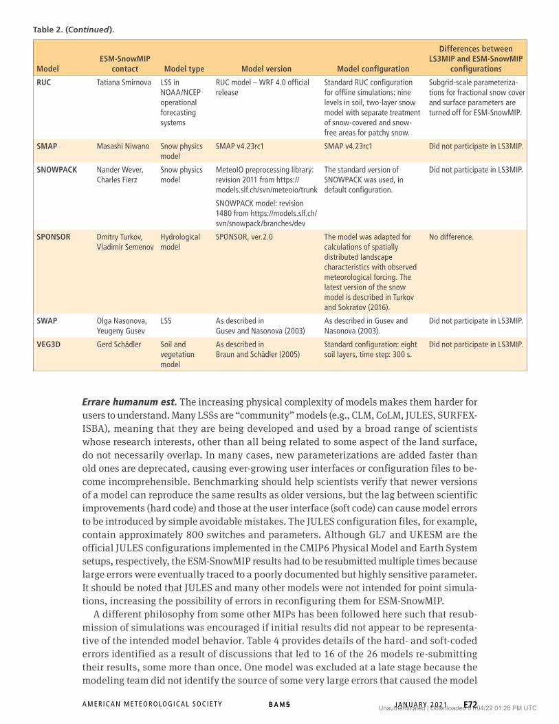
Errare humanum est. The increasing physical complexity of models makes them harder for users to understand. Many LSSs are “community” models (e.g., CLM, CoLM, JULES, SURFEX-ISBA), meaning that they are being developed and used by a broad range of scientists whose research interests, other than all being related to some aspect of the land surface, do not necessarily overlap. In many cases, new parameterizations are added faster than old ones are deprecated, causing ever-growing user interfaces or configuration files to be-come incomprehensible. Benchmarking should help scientists verify that newer versions of a model can reproduce the same results as older versions, but the lag between scientific improvements (hard code) and those at the user interface (soft code) can cause model errors to be introduced by simple avoidable mistakes. The JULES configuration files, for example, contain approximately 800 switches and parameters. Although GL7 and UKESM are the official JULES configurations implemented in the CMIP6 Physical Model and Earth System setups, respectively, the ESM-SnowMIP results had to be resubmitted multiple times because large errors were eventually traced to a poorly documented but highly sensitive parameter. It should be noted that JULES and many other models were not intended for point simula-tions, increasing the possibility of errors in reconfiguring them for ESM-SnowMIP.

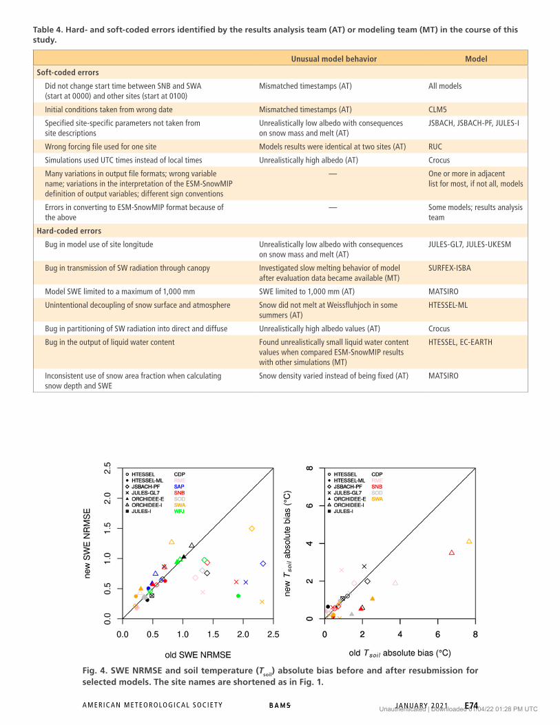
A different philosophy from some other MIPs has been followed here such that resub-mission of simulations was encouraged if initial results did not appear to be representa-tive of the intended model behavior. Table 4 provides details of the hard- and soft-coded errors identified as a result of discussions that led to 16 of the 26 models re-submitting their results, some more than once. One model was excluded at a late stage because the modeling team did not identify the source of some very large errors that caused the model

ModelESM-SnowMIP

contact Model type Model version Model configuration

Differences between LS3MIP and ESM-SnowMIP

configurations

RUC Tatiana Smirnova LSS in NOAA/NCEP operational forecasting systems

RUC model – WRF 4.0 official release

Standard RUC configuration for offline simulations: nine levels in soil, two-layer snow model with separate treatment of snow-covered and snow- free areas for patchy snow.

Subgrid-scale parameteriza-tions for fractional snow cover and surface parameters are turned off for ESM-SnowMIP.

SMAP Masashi Niwano Snow physics model

SMAP v4.23rc1 SMAP v4.23rc1 Did not participate in LS3MIP.

SNOWPACK Nander Wever, Charles Fierz

Snow physics model

MeteoIO preprocessing library: revision 2011 from https:// models.slf.ch/svn/meteoio/trunk

The standard version of SNOWPACK was used, in default configuration.

Did not participate in LS3MIP.

SNOWPACK model: revision 1480 from https://models.slf.ch/ svn/snowpack/branches/dev

SPONSOR Dmitry Turkov, Vladimir Semenov

Hydrological model

SPONSOR, ver.2.0 The model was adapted for calculations of spatially distributed landscape characteristics with observed meteorological forcing. The latest version of the snow model is described in Turkov and Sokratov (2016).

No difference.

SWAP Olga Nasonova, Yeugeny Gusev

LSS As described in Gusev and Nasonova (2003)

As described in Gusev and Nasonova (2003).

Did not participate in LS3MIP.

VEG3D Gerd Schädler Soil and vegetation model

As described in Braun and Schädler (2005)

Standard configuration: eight soil layers, time step: 300 s.

Did not participate in LS3MIP.

Table 2. (Continued).

Unauthenticated | Downloaded 01/04/22 01:28 PM UTC

A M E R I C A N M E T E O R O L O G I C A L S O C I E T Y J A N UA RY 2 0 2 1 E73

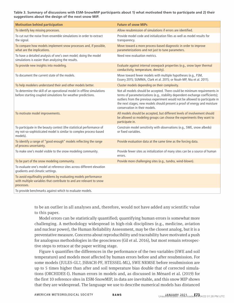
Table 3. Summary of discussions with ESM-SnowMIP participants about 1) what motivated them to participate and 2) their suggestions about the design of the next snow MIP.

Motivation behind participation Future of snow MIPs

To identify key missing processes. Allow resubmission of simulations if errors are identified.

To cut out the noise from ensemble simulations in order to extract the signal.

Provide model code and initialization files as well as model results for transparency.

To compare how models implement snow processes and, if possible, what are the implications.

Move toward a more process-based diagnostic in order to improve parameterizations and not just to tune parameters.

To have a detailed analysis of one’s own model; doing the model simulations is easier than analyzing the results.

Need new evaluation metrics.

To provide new insights into modeling. Evaluate against internal snowpack properties (e.g., snow layer thermal conductivity, temperature, density).

To document the current state of the models. Move toward fewer models with multiple hypotheses (e.g., FSM, Essery 2015; SUMMA, Clark et al. 2015; or Noah-MP, Niu et al. 2011).

To help modelers understand their and other models better. Cluster models depending on their complexity.

To determine the skill of an operational model in offline simulations before starting coupled simulations for weather predictions.

Not all models should be accepted. There could be minimum requirements in terms of parameterizations (e.g., stability dependent exchange coefficients); outliers from the previous experiment would not be allowed to participate in the next stages; new models should present a proof of energy and moisture conservation in their models.

To motivate model improvements. All models should be accepted, but different levels of involvement should be allowed so modeling groups can choose the experiments they want to participate in.

To participate in the beauty contest (the statistical performance of my not-so-sophisticated model is similar to complex process-based models).

Constrain model sensitivity with observations (e.g., SWE, snow albedo) or fixed variables.

To identify a range of “good enough” models reflecting the range of process uncertainty.

Provide evaluation data at the same time as the forcing data.

To make one’s model visible to the snow modeling community. Provide fewer sites as initialization of many sites can be a source of human errors.

To be part of the snow modeling community. Provide more challenging sites (e.g., tundra, wind-blown).

To evaluate one’s model at reference sites across different elevation gradients and climatic settings.

To avoid equifinality problems by evaluating models performance with multiple variables that contribute to and are relevant to snow processes.

To provide benchmarks against which to evaluate models.

to be an outlier in all analyses and, therefore, would not have added any scientific value to this paper.

Model errors can be statistically quantified; quantifying human errors is somewhat more challenging. A methodology widespread in high-risk disciplines (e.g., medicine, aviation and nuclear power), the Human Reliability Assessment, may be the closest analog, but it is a preventative measure. Concerns about reproducibility and traceability have motivated a push for analogous methodologies in the geosciences (Gil et al. 2016), but most remain retrospec-tive steps to retrace at the paper writing stage.

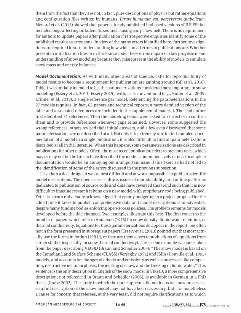
Figure 4 quantifies the differences in the performance of the two variables (SWE and soil temperature) and models most affected by human errors before and after resubmission. For some models (JULES-GL7, JSBACH-PF, HTESSEL-ML), SWE NRMSE before resubmission are up to 5 times higher than after and soil temperature bias double that of corrected simula-tions (ORCHIDEE-I). Human errors in models and, as discussed in Ménard et al. (2019) for the first 10 reference sites in ESM-SnowMIP, in data are inevitable, and this snow MIP shows that they are widespread. The language we use to describe numerical models has distanced

Unauthenticated | Downloaded 01/04/22 01:28 PM UTC

A M E R I C A N M E T E O R O L O G I C A L S O C I E T Y J A N UA RY 2 0 2 1 E74

Table 4. Hard- and soft-coded errors identified by the results analysis team (AT) or modeling team (MT) in the course of this study.

Unusual model behavior Model

Soft-coded errors

Did not change start time between SNB and SWA (start at 0000) and other sites (start at 0100)

Mismatched timestamps (AT) All models

Initial conditions taken from wrong date Mismatched timestamps (AT) CLM5

Specified site-specific parameters not taken from site descriptions

Unrealistically low albedo with consequences on snow mass and melt (AT)

JSBACH, JSBACH-PF, JULES-I

Wrong forcing file used for one site Models results were identical at two sites (AT) RUC

Simulations used UTC times instead of local times Unrealistically high albedo (AT) Crocus

Many variations in output file formats; wrong variable name; variations in the interpretation of the ESM-SnowMIP definition of output variables; different sign conventions

— One or more in adjacent list for most, if not all, models

Errors in converting to ESM-SnowMIP format because of the above

— Some models; results analysis team

Hard-coded errors

Bug in model use of site longitude Unrealistically low albedo with consequences on snow mass and melt (AT)

JULES-GL7, JULES-UKESM

Bug in transmission of SW radiation through canopy Investigated slow melting behavior of model after evaluation data became available (MT)

SURFEX-ISBA

Model SWE limited to a maximum of 1,000 mm SWE limited to 1,000 mm (AT) MATSIRO

Unintentional decoupling of snow surface and atmosphere Snow did not melt at Weissfluhjoch in some summers (AT)

HTESSEL-ML

Bug in partitioning of SW radiation into direct and diffuse Unrealistically high albedo values (AT) Crocus

Bug in the output of liquid water content Found unrealistically small liquid water content values when compared ESM-SnowMIP results with other simulations (MT)

HTESSEL, EC-EARTH

Inconsistent use of snow area fraction when calculating snow depth and SWE

Snow density varied instead of being fixed (AT) MATSIRO

Fig. 4. SWE NRMSE and soil temperature (Tsoil) absolute bias before and after resubmission for selected models. The site names are shortened as in Fig. 1.

Unauthenticated | Downloaded 01/04/22 01:28 PM UTC

A M E R I C A N M E T E O R O L O G I C A L S O C I E T Y J A N UA RY 2 0 2 1 E75

them from the fact that they are not, in fact, pure descriptions of physics but rather equations and configuration files written by humans. Errare humanum est, perseverare diabolicum. Ménard et al. (2015) showed that papers already published had used versions of JULES that included bugs affecting turbulent fluxes and causing early snowmelt. There is no requirement for authors to update papers after publication if retrospective enquiries identify some of the published results as erroneous. In view of the many errors identified here, further investiga-tions are required to start understanding how widespread errors in publications are. Whether present in initialization files or in the source code, these errors impair or slow progress in our understanding of snow modeling because they misrepresent the ability of models to simulate snow mass and energy balances.

Model documentation. As with many other areas of science, calls for reproducibility of model results to become a requirement for publication are gaining ground (Gil et al. 2016). Table 1 was initially intended to list the parameterizations considered most important in snow modeling (Essery et al. 2013; Essery 2015), with, as is conventional (e.g., Rutter et al. 2009; Krinner et al. 2018), a single reference per model. Referencing the parameterizations in the 27 models requires, in fact, 63 papers and technical reports; a more detailed version of the table and associated references are included in the supplemental material. The lead author first identified 51 references. Then the modeling teams were asked to correct or to confirm them and to provide references whenever gaps remained. However, some suggested the wrong references, others revised their initial answers, and a few even discovered that some parameterizations are not described at all. Not only is it extremely rare to find complete docu-mentation of a model in a single publication, it is also difficult to find all parameterizations described at all in the literature. When this happens, some parameterizations are described in publications for other models. Often, the most recent publication refers to previous ones, which may or may not be the first to have described the model, comprehensively or not. Incomplete documentation would be an annoying but unimportant issue if this exercise had not led to the identification of some of the errors discussed in the previous subsection.

Less than a decade ago, it was at best difficult and at worst impossible to publish scientific model descriptions. The open access culture, issues of reproducibility, and online platforms dedicated to publication of source code and data have reversed this trend such that it is now difficult to imagine research relying on a new model with proprietary code being published. Yet, it is a truth universally acknowledged that openly budgeting in a project proposal for the added time it takes to publish comprehensive data and model descriptions is unadvisable, despite many funding bodies enforcing open-access policies. The problem remains for models developed before the tide changed. Two examples illustrate this best. The first concerns the number of papers which refer to Anderson (1976) for snow density, liquid water retention, or thermal conductivity. Equations for these parameterizations do appear in the report, but often not in the form presented in subsequent papers [Essery et al. (2013) pointed out that most actu-ally use the forms in Jordan (1991)], or they are themselves reproductions of equations from earlier studies (especially for snow thermal conductivity). The second example is a quote taken from the paper describing VEG3D (Braun and Schädler 2005): “The snow model is based on the Canadian Land Surface Scheme (CLASS) (Verseghy 1991) and ISBA (Douville et al. 1995) models, and accounts for changes of albedo and emissivity as well as processes like compac-tion, destructive metamorphosis, the melting of snow, and the freezing of liquid water.” This sentence is the only description in English of the snow model in VEG3D; a more comprehensive description, not referenced in Braun and Schädler (2005), is available in German in a PhD thesis (Grabe 2002). The study in which the quote appears did not focus on snow processes, so a full description of the snow model may not have been necessary, but it is nonetheless a cause for concern that referees, at the very least, did not require clarifications as to which

Unauthenticated | Downloaded 01/04/22 01:28 PM UTC

A M E R I C A N M E T E O R O L O G I C A L S O C I E T Y J A N UA RY 2 0 2 1 E76

processes were based on CLASS and which on ISBA. Changes in emissivity certainly were not based on either model as both did—and still do—have fixed emissivity. This is the most succinct description of a snow model, but not the only one to offer little or no information about process representations. At the other end of the spectrum, the CLM5 documentation is the most comprehensive and makes all the information available in a single technical report (Lawrence et al. 2020). A few models follow closely with most information being available in a single document that clearly references where to obtain additional information (e.g., CLASS, SURFEX-ISBA, HTESSEL, JULES, SNOWPACK). The “publish or perish” culture is estimated to foster a 9% yearly growth rate in scientific publications (Bornmann and Mutz 2015), which will be matched by a comparable rate of solicitations for peer reviewing. Whether it is because we do not take or have time to fact-check references, the current peer-review process is failing when poorly described models are published. The aim of LS3MIP and ESM-SnowMIP is to investigate systematic errors in models; errors can be quantified against evaluation data for any model, but poor documentation accentuates our poor understanding of model behavior and reduces MIPs to statistical exercises rather than to insightful studies.

What the future holdsHistorically, PILPS (Henderson-Sellers et al. 1995) and other intercomparison projects have provided platforms to motivate model developments; they are now inextricably linked to suc-cessive IPCC reports. In view of heavily mediatized errors such as the claim that Himalayan glaciers would melt by 2035—interestingly described as “human error” by the then IPCC chair-man Rajendra Pachauri (IPCC 2010; Times of India 2010)—we must reflect on how damaging potential errors are to the climate science community. Not only are the IPCC reports the most authoritative in international climate change policy-making, but they have become—for better or worse—proxies for the credibility of climate scientists to the general public. It is therefore time that we reflect on our community and openly acknowledge that some model uncertain-ties cannot be quantified at present because they are due to human errors.

Other factors are also responsible for the modeling of snow processes not having progressed as fast as other areas relying on technology. Discussions on the future of snow MIPs involving organizers and participants of ESM-SnowMIP issued from this study. As in the discussion about motivation of participants, suggestions for the design of future MIPs were varied, and at times contradictory, but responses from participants reflected the purpose their models serve (Table 4). The IPCC Expert Meeting on Multi Model Evaluation Good Practice Guidance states that “there should be no minimum performance criteria for entry into the CMIP multimodel database. Researchers may select a subset of models for a particular analysis but should docu-ment the reasons why” (Knutti et al. 2010). Nevertheless, many participants argued that the “one size fits all” approach should be reconsidered. ESM-SnowMIP evaluated models against the same bulk snowpack properties as previous snow MIPs. This suited LSSs that represent snow as a composite snow–soil layer or as a single layer, but there is a demand for more com-plex models that simulate profiles of internal snowpack properties to be evaluated against data that match the scale of the processes they represent (e.g., snow layer temperatures, liquid water content, and microstructure). Models used at very high resolution for avalanche risk forecasting (such as Crocus and SNOWPACK; Morin et al. 2020) and by the tourism industry are constantly being tested during the snow season, and errors can cost lives and money. However, obtaining reliable data and designing appropriate evaluation methodologies to drive progress in complex snow models is challenging (Ménard et al. 2019). For example, solving the trade-off between SWE and surface temperature errors requires more measurements of surface mass and energy balance components: simple in theory but expensive and logisti-cally difficult in practice. The scale at which even the more complex models operate is also impeding progress. Until every process can be described explicitly, the reliance of models

Unauthenticated | Downloaded 01/04/22 01:28 PM UTC

A M E R I C A N M E T E O R O L O G I C A L S O C I E T Y J A N UA RY 2 0 2 1 E77

on parameterizations to describe very small scale processes (such as the surface exchanges upon which the above trade-off depends) are inevitable sources of uncertainty.

Despite expressing a need for change in the design of snow MIPs, many participants de-scribed ESM-SnowMIP as a success because it allowed them to identify bugs or areas of their models in need of further improvements; some improvements were implemented in the course of this study, others are in development. Ultimately, ESM-SnowMIP’s main flaw is of not being greater than the sum of its parts. Its working hypothesis was not supported and, per se, has failed to advance our understanding of snow processes. However, the collaborative effort allowed us to report a false, but plausible hypothesis, to expose our misplaced assumptions and to reveal a disparity of opinions on the purpose, design and future of snow MIPs. In view of our findings, of the time investment required of participating modelers and of novel ways to utilize already available global-scale simulations (e.g., Mudryk et al. 2020), most planned ESM-SnowMIP experiments may not go ahead, but site simulations with evaluation data covering bulk and internal snowpack properties will be expanded. Learning from our mistakes to implement future MIPs may yet make it an unqualified success in the long term.

Acknowledgments. CM and RE were supported by NERC Grant NE/P011926/1. Simulations by partici-pating models were supported by the following programs and grants: Capability Development Fund of CSIRO Oceans and Atmosphere, Australia (CABLE); Canada Research Chairs and Global Water Futures (CRHM); H2020 APPLICATE Grant 727862 (HTESSEL); Met Office Hadley Centre Climate Programme by BEIS and Defra (JULES-UKESM and GL7); TOUGOU Program from MEXT, Japan (MATSIRO); RUC by NOAA Grant NOAA/NA17OAR4320101 (RUC); Russian Foundation for Basic Research Grant 18-05-60216 (SPONSOR); and Russian Science Foundation Grant 16-17-10039 (SWAP). ESM-SnowMIP was supported by the World Climate Research Programme’s Climate and Cryosphere (CliC) core project.

Unauthenticated | Downloaded 01/04/22 01:28 PM UTC

A M E R I C A N M E T E O R O L O G I C A L S O C I E T Y J A N UA RY 2 0 2 1 E78

References

Anderson, E. A., 1976: A point energy and mass balance model of a snow cover. NOAA Tech. Rep. NWS 19, 150 pp., https://repository.library.noaa.gov/view/noaa/6392.

Arduini, G., G. Balsamo, E. Dutra, J. J. Day, I. Sandu, S. Boussetta, and T. Haiden, 2019: Impact of a multi‐layer snow scheme on near‐surface weather forecasts. J. Adv. Model. Earth Syst., 11, 4687–4710, https://doi.org/10.1029/2019MS001725.

Baartman, J. E. M., L. A. Melsen, D. Moore, and M. J. van der Ploeg, 2020: On the complexity of model complexity: Viewpoints across the geosciences. Catena, 186, 104261, https://doi.org/10.1016/j.catena.2019.104261.

Best, M. J., and Coauthors, 2011: The Joint UK Land Environment Simulator (JULES), model description – Part 1: Energy and water fluxes. Geosci. Model Dev., 4, 677–699, https://doi.org/10.5194/gmd-4-677-2011.

Bornmann, L., and R. Mutz, 2015: Growth rates of modern science: A bibliometric analysis based on the number of publications and cited references. J. Assoc. Inf. Sci. Technol., 66, 2215–2222, https://doi.org/10.1002/asi.23329.

Braun, F. J., and G. Schädler, 2005: Comparison of soil hydraulic parameteriza-tions for mesoscale meteorological models. J. Appl. Meteor., 44, 1116–1132, https://doi.org/10.1175/JAM2259.1.

Clark, M. P., and Coauthors, 2015: A unified approach for process-based hydro-logic modeling: 1. Modeling concept. Water Resour. Res., 51, 2498–2514, https://doi.org/10.1002/2015WR017198.

Conway, J. P., J. W. Pomeroy, W. D. Helgason, and N. J. Kinar, 2018: Challenges in modelling turbulent heat fluxes to snowpacks in forest clearings. J. Hydrome-teor., 19, 1599–1616, https://doi.org/10.1175/JHM-D-18-0050.1.

Cox, P. M., R. A. Betts, C. Bunton, R. Essery, P. R. Rowntree, and J. Smith, 1999: The impact of new land surface physics on the GCM simulation of climate and climate sensitivity. Climate Dyn., 15, 183–203, https://doi.org/10.1007/s003820050276.

Cuntz, M., and V. Haverd, 2018: Physically accurate soil freeze-thaw processes in a global land surface scheme. J. Adv. Model. Earth Syst., 10, 54–77, https://doi.org/10.1002/2017MS001100.

Decharme, B., E. Brun, A. Boone, C. Delire, P. Le Moigne, and S. Morin, 2016: Impacts of snow and organic soils parameterization on northern Eurasian soil temperature profiles simulated by the ISBA land surface model. Cryosphere, 10, 853–877, https://doi.org/10.5194/tc-10-853-2016.

Douville, H., J.-F. Royer, and J.-F. Mahouf, 1995: A new snow parameterization for the Meteo-France climate model. Part I: Validation in stand-alone experi-ments. Climate Dyn., 12, 21–35, https://doi.org/10.1007/BF00208760.

Dutra, E., G. Balsamo, P. Viterbo, P. M. A. Miranda, A. Beljaars, C. Schär, and K. Elder, 2010: An improved snow scheme for the ECMWF land surface model: Description and offline validation. J. Hydrometeor., 11, 899–916, https://doi.org/10.1175/2010JHM1249.1.

Ekici, A., C. Beer, S. Hagemann, J. Boike, M. Langer, and C. Hauck, 2014: Simulating high-latitude permafrost regions by the JSBACH terrestrial ecosystem model. Geosci. Model Dev., 7, 631–647, https://doi.org/10.5194/gmd-7-631-2014.

Essery, R., 2013: Large-scale simulations of snow albedo masking by forests. Geophys. Res. Lett., 40, 5521–5525, https://doi.org/10.1002/grl.51008.

—, 2015: A Factorial Snowpack Model (FSM 1.0). Geosci. Model Dev., 8, 3867–3876, https://doi.org/10.5194/gmd-8-3867-2015.

—, and Coauthors, 2009: SNOWMIP2: An evaluation of forest snow process simulations. Bull. Amer. Meteor. Soc., 90, 1120–1136, https://doi.org/10.1175 /2009BAMS2629.1.

—, S. Morin, Y. Lejeune, and C. Menard, 2013: A comparison of 1701 snow models using observations from an alpine site. Adv. Water Resour., 55, 131–148, https://doi.org/10.1016/j.advwatres.2012.07.013.

Etchevers, P., and Coauthors, 2002: SnowMiP, an intercomparison of snow mod-els: First results. Proc. Int. Snow Science Workshop, Penticton, Canada, Inter-national Snow Science Workshop, 353–360.

—, and Coauthors, 2004: Validation of the energy budget of an alpine snow-pack simulated by several snow models (Snow MIP project). Ann. Glaciol., 38, 150–158, https://doi.org/10.3189/172756404781814825.

Flato, G., and Coauthors, 2013: Evaluation of climate models. Climate Change 2013: The Physical Science Basis, T. F. Stocker et al., Eds., Cambridge University Press, 741–866.

Gil, Y., and Coauthors, 2016: Toward the Geoscience Paper of the Future: Best prac-tices for documenting and sharing research from data to software to prove-nance. Earth Space Sci., 3, 388–415, https://doi.org/10.1002/2015EA000136.

Guimberteau, M., and Coauthors, 2018: ORCHIDEE-MICT (v8.4.1), a land surface model for the high latitudes: Model description and validation. Geosci. Model Dev., 11, 121–163, https://doi.org/10.5194/gmd-11-121-2018.

Grabe, F., 2002: Simulation der Wechselwirkung zwischen Atmosphäre, Veg-etation und Erdoberfläche bei Verwendung unterschiedlicher Parametrisier-ungsansätze. Ph.D. thesis, Karlsruhe University, 218 pp.

Gusev, Y. M., and O. N. Nasonova, 2003: The simulation of heat and water exchange in the boreal spruce forest by the land-surf ace model SWAP. J. Hydrol., 280, 162–191, https://doi.org/10.1016/S0022-1694(03)00221-X.

Haverd, V., M. Cuntz, L. P. Nieradzik, and I. N. Harman, 2016: Improved represen-tations of coupled soil–canopy processes in the CABLE land surface model (Subversion revision 3432). Geosci. Model Dev., 9, 3111–3122, https://doi.org/10.5194/gmd-9-3111-2016.

Henderson-Sellers, A., A. J. Pitman, P. K. Love, P. Irannejad, and T. Chen, 1995: The Project for Intercomparison of Land Surface Parameterization Schemes (PILPS): Phases 2 and 3. Bull. Amer. Meteor. Soc., 76, 489–503, https://doi.org/10.1175/1520-0477(1995)076<0489:TPFIOL>2.0.CO;2.

Hitchcock, A., Dir., 1960: Psycho. Paramount Pictures, film, 109 min.IPCC, 2010: IPCC statement on the melting of Himalayan glaciers. Accessed on 29

October 2019, https://archive.ipcc.ch/pdf/presentations/himalaya-statement-20january2010.pdf.

Jordan, R., 1991: A one-dimensional temperature model for a snow cover: Technical documentation for SNTHERM.89. Special Rep. 91-16, Cold Region Research and Engineers Laboratory, U.S. Army Corps of Engineers, Hanover, NH, 62 pp.

Kerr, N. L., 1998: HARKing: Hypothesizing after the results are known. Pers. Soc. Psychol. Rev., 2, 196–217, https://doi.org/10.1207/s15327957pspr0203_4.

Knutti, R., G. Abramowitz, M. Collins, V. Eyring, P. J. Gleckler, B. Hewitson, and L. Mearns, 2010: Good practice guidance paper on assessing and combining multi model climate projections. T. F. Stocker et al., Eds., IPCC, 15 pp., https://wg1.ipcc.ch/docs/IPCC_EM_MME_GoodPracticeGuidancePaper.pdf.

Krinner, G., and Coauthors, 2018: ESM-SnowMIP: Assessing snow models and quantifying snow-related climate feedbacks. Geosci. Model Dev., 11, 5027–5049, https://doi.org/10.5194/gmd-11-5027-2018.

Lafaysse, M., B. Cluzet, M. Dumont, Y. Lejeune, V. Vionnet, and S. Morin, 2017: A multiphysical ensemble system of numerical snow modelling. Cryosphere, 11, 1173–1198, https://doi.org/10.5194/tc-11-1173-2017.

Lawrence, D., and Coauthors, 2020: Technical description of version 5.0 of the Community Land Model (CLM). NCAR Tech. Note, 329 pp., www.cesm.ucar.edu/models/cesm2/land/CLM50_Tech_Note.pdf.

Lee, R., D. Greene, and P. House, 1977: The ‘false consensus effect’: An egocentric bias in social perception and attribution processes. J. Exp. Soc. Psychol., 13, 279–301, https://doi.org/10.1016/0022-1031(77)90049-X.

Li, Y., T. Wang, Z. Zeng, S. Peng, X. Lian, and S. Piao, 2016: Evaluating biases in simulated land surface albedo from CMIP5 global climate models. J. Geophys. Res. Atmos., 121, 6178–6190, https://doi.org/10.1002/2016JD024774.

Martin, G. R. R., 1996: A Game of Thrones. Bantam Spectra, 835 pp.Ménard, C. B., J. Ikonen, K. Rautiainen, M. Aurela, A. N. Arslan, and J. Pulliainen,

2015: Effects of meteorological and ancillary data, temporal averaging, and evaluation methods on model performance and uncertainty in a land sur-face model. J. Hydrometeor., 16, 2559–2576, https://doi.org/10.1175/JHM-D-15-0013.1.

—, and Coauthors, 2019: Meteorological and evaluation datasets for snow modelling at 10 reference sites: Description of in situ and bias-corrected reanalysis data. Earth Syst. Sci. Data, 11, 865–880, https://doi.org/10.5194/essd-11-865-2019.

Unauthenticated | Downloaded 01/04/22 01:28 PM UTC

A M E R I C A N M E T E O R O L O G I C A L S O C I E T Y J A N UA RY 2 0 2 1 E79

Morin, S., and Coauthors, 2020: Application of physical snowpack models in sup-port of operational avalanche hazard forecasting: A status report on current implementations and prospects for the future. Cold Reg. Sci. Technol., 170, 102910, https://doi.org/10.1016/j.coldregions.2019.102910.

Mudryk, L., M. Santolaria-Otín, G. Krinner, M. Ménégoz, C. Derksen, C. Brutel-Vuilmet, M. Brady, and R. Essery, 2020: Historical Northern Hemisphere snow cover trends and projected changes in the CMIP6 multi-model ensemble. Cryosphere, 14, 2495–2514, https://doi.org/10.5194/tc-14-2495-2020.

Munafò, M., and Coauthors, 2017: A manifesto for reproducible science. Nat. Hum. Behav., 1, 0021, https://doi.org/10.1038/s41562-016-0021.

Niu, G.-Y., and Coauthors, 2011: The community NOAH land surface model with multiparameterization options (NOAH-MP): 1. Model description and evalu-ation with local-scale measurements. J. Geophys. Res., 116, D12109, https://doi.org/10.1029/2010JD015139.

Pitman, A. J., and A. Henderson-Sellers, 1998: Recent progress and results from the project for the intercomparison of land surface parameterization schemes. J. Hydrol., 212–213, 128–135, https://doi.org/10.1016/S0022-1694(98)00206-6.

Pomeroy, J. W., X. Fang, and C. Ellis, 2012: Sensitivity of snowmelt hydrology in Marmot Creek, Alberta, to forest cover disturbance. Hydrol. Processes, 26, 1891–1904, https://doi.org/10.1002/hyp.9248.

Randall, D. A., and Coauthors, 2007: Climate models and their evaluation. Climate Change 2007: The Physical Science Basis, S. Solomon et al., Eds., Cambridge University Press, 589–662.

Roesch, A., 2006: Evaluation of surface albedo and snow cover in AR4 coupled climate models. J. Geophys. Res., 111, D15111, https://doi.org/10.1029/ 2005JD006473.

Rutter, N., and Coauthors, 2009: Evaluation of forest snow processes models (Snow-MIP2). J. Geophys. Res., 114, D06111, https://doi.org/10.1029/2008JD011063.

Sandu, I., A. Beljaars, P. Bechtold, T. Mauritsen, and G. Balsamo, 2013: Why is it so difficult to represent stably stratified conditions in numerical weather

prediction (NWP) models? J. Adv. Model. Earth Syst., 5, 117–133, https://doi.org/10.1002/jame.20013.

Scott, R., Dir., 1979: Alien. 20th Century Fox, film, 117 min.Slater, A. G., and Coauthors, 2001: The representation of snow in land surface

schemes: Results from PILPS 2(d). J. Hydrometeor., 2, 7–25, https://doi.org/10.1175/1525-7541(2001)002<0007:TROSIL>2.0.CO;2.

Times of India, 2010: Pachauri admits mistake in IPCC report. Times of India, 23 January, accessed 4 October 2019, https://timesofindia.indiatimes.com/videos/news/Pachauri-admits-mistake-in-IPCC-report/videoshow/5492814.cms.

Turkov, D. V., and V. S. Sokratov, 2016: Calculating of snow cover characteristics on a plain territory using the model SPONSOR and data of reanalyses (by the example of Moscow region) (in Russian). J. Ice Snow, 56, 369–380, https://doi.org/10.15356/2076-6734-2016-3-369-380.

van den Hurk, B., and Coauthors, 2016: LS3MIP (v1.0) contribution to CMIP6: The land surface, snow and soil moisture model intercomparison project—Aims, setup and expected outcome. Geosci. Model Dev., 9, 2809–2832, https://doi.org/10.5194/gmd-9-2809-2016.

Verseghy, D. L., 1991: CLASS—A Canadian land surface scheme for GCMS. I. Soil model. Int. J. Climatol., 11, 111–133, https://doi.org/10.1002/joc. 3370110202.

Wang, L., J. N. S. Cole, P. Bartlett, D. Verseghy, C. Derksen, R. Brown, and K. von Salzen, 2016: Investigating the spread in surface albedo for snow-covered forests in CMIP5 models. J. Geophys. Res. Atmos., 121, 1104–1119, https://doi.org/10.1002/2015JD023824.

Wang, T., and Coauthors, 2013: Evaluation of an improved intermediate com-plexity snow scheme in the ORCHIDEE land surface model. J. Geophys. Res. Atmos., 118, 6064–6079, https://doi.org/10.1002/jgrd.50395.

Weber, M., 2008: A parameterization for the turbulent fluxes over melting sur-faces derived from eddy correlation measurements. Proc. Alpine Snow Work-shop, Munich, Germany, Nationalpark Berchtesgaden, 138–149.

Unauthenticated | Downloaded 01/04/22 01:28 PM UTC