1

SCIENTIFIC COMMITTEE

FIFTH REGULAR SESSION

10-21 August 2009

Port Vila, Vanuatu

UPDATE OF RECENT DEVELOPMENTS IN MULTIFAN-CL AND RELATED

SOFTWARE FOR STOCK ASSESSMENT

WCPFC-SC5-2009/SA- IP-07

Simon Hoyle1, Dave Fournier

2, Pierre Kleiber

3, John Hampton

1, Fabrice Bouyé

1, Nick Davies

1,

and Shelton Harley1

1 Oceanic Fisheries Programme, Secretariat of the Pacific Community, Noumea, New Caledonia 2 Otter Research Ltd 3 Islands Fisheries Science Center, National Marine Fisheries Service, Honolulu, Hawaii, USA.

2

Update of recent developments in MULTIFAN-CL and related software for stock assessment

Simon Hoyle, Dave Fournier, Pierre Kleiber, John Hampton, Fabrice Bouyé, Nick Davies

and Shelton Harley.

Introduction MULTIFAN-CL (MFCL) is a statistical, age-structured, length-based model routinely used

for stock assessments of tuna and other pelagic species. The model was originally developed

by Dave Fournier of Otter Research for application to south Pacific albacore tuna.

MFCL is typically fitted to total catch, size-frequency and tagging data stratified by fishery,

region and time period. Recent tropical tuna assessments (e.g. Langley et al. 2007; Langley et

al. 2008) encompass a time period of 1952–2007 in quarterly time steps, and model >20

separate fisheries occurring in 6 spatial regions. The main parameters estimated by the model

include initial numbers-at-age in each region (constrained by an equilibrium age-structure

assumption), the number in age class 1 for each quarter in each region (the recruitment),

growth parameters, natural mortality-at-age (if estimated), selectivity-at-age by fishery

(constrained by smoothing penalties or splines), effort deviations (random variations in the

effort-fishing mortality relationship) for each fishery, initial catchability and catchability

deviations (cumulative changes in catchability with time) for each fishery (if estimated).

Parameters are estimated by fitting to a composite likelihood comprised of the fits to the data

and prior distributions for various parameters.

Each year the MFCL development team work to improve the model to accommodate changes

in understanding of the fishery, to fix software errors, and to improve usability. This

document records changes made since August 2007 to the model and to the other components

of the MFCL project.

Development overview

Team The senior developer of MFCL is Dave Fournier, of Otter Software in Canada. Occasional

programming is carried out by Pierre Kleiber (NMFS Hawaii), Simon D Hoyle, Nick Davies,

and John Hampton (all SPC, New Caledonia). Other tasks include testing and debugging

(SDH, ND, PK, JH, and Fabrice Bouye (SPC)); documentation (PK, SDH); and planning and

coordination (SDH, JH, Shelton Harley). Related project software are developed or managed

by FB (MFCL Viewer, Condor, Gforge), PK (R scripts), and SDH (R4MFCL, Condor).

Calendar September – December: Planning and ongoing code development

January: MFCL development meeting, 1-4 weeks

February – March: Testing and finalizing production version

April-July: Stock assessments

3

MFCL collaboration and versioning We have established a project management website based on the open source Gforge

software. It is used to report problems, list and document potential enhancements, and to

allocate tasks. It also hosts a code repository.

The code repository for MFCL development uses the open source software SVN. This

repository keeps track of different versions of the software, and allows our international team

of developers to merge different versions of the software. The repository is held at SPC, but

is accessible via the internet to the development team. The repository and overall

development are coordinated via the GForge website http://gforge2.spc.int/. This website is

administered by Fabrice Bouye fabriceb@spc.int.

Tool development 1. The libraries of R scripts written by Pierre Kleiber have been updated so that they

now work in a standard Windows installation, as well as in Linux as they did before.

2. A new set of R scripts for working with MFCL has been developed and released on

the internet at the following URL: http://code.google.com/p/r4mfcl/. These scripts are

used to manipulate the input files, so that runs can be automated. Other scripts can be

used to read in the output files, analyze the results, and generate plots and tables. See

Table 4 for a list of these R scripts. Further development is planned to provide a

comprehensive environment, within which the routine aspects of stock assessments

can be automated.

3. The MFCL viewer has been updated with a new residual plot. It has also been

modified to deal with new versions of the MFCL output files.

4. Condor (www.condor.wisc.edu), a tool for high throughput computing, as been used

to manage a grid currently numbering 50 processors. We have written scripts to

enable it to run MFCL. R, and Stock synthesis. This enables multiple jobs to be run in

a short time. It is currently used for running the stock assessments, and for the

structural sensitivity analysis. It could also be used for other computer intensive tasks

such as management strategy evaluation.

MFCL manual The MFCL manual has been converted by Pierre Kleiber from LaTeX to Microsoft Word

2007. This change will enable more people to work on the manual, and we hope that it will

accelerate the process of updating it. The manual has also been added to the SVN repository,

to ensure that changes are distributed to the development team in a timely way. Recent

updates include adding information about length-specific selectivity and parallelizing the

Hessian. However, many further changes are still required.

4

New MFCL features

Length-based selectivity The most significant change to MFCL since 2007 has been the addition of length-based

selectivity. Recent stock assessments have noted problems fitting to size frequency data (e.g.

bigeye assessment). A comparative analysis (Hoyle and Langley 2007) using Stock Synthesis

(Methot 2007) suggested that size-based selectivity could give a better fit to the data.

Need

Fishery selectivity is in many cases a size-based process. Fish behavior, and hence

vulnerability to fishing, may change with size. Some gear types are also inherently size-

selective. To date, MFCL has defined selectivity by fishery in terms of age. It has had a

selectivity option sometimes referred to as „length-based selectivity‟, but this implementation

was limited in scope – it constrained selectivity of age classes to be similar, to the extent that

their length distributions were similar. The expected distribution of catch at length was still

calculated by multiplying catch at age by the distribution of length at age.

Age-based selectivity tends to be an approximation to real-world fishery selectivity, because

of the implicit assumption that all fish of the same age are selected at the same rate. It will

give different results from length-based selectivity, to the extent that the observed distribution

of catch at size includes some of the lengths within an age class, but not others. The

importance of these effects is greater in some fisheries than others.

The bigeye stock assessment (Langley et al. 2008) may have been affected by the way the

selectivity is modeled in the Chinese/Chinese Taipei longline fisheries. The size data in these

fisheries appears to be driving the observed increasing recruitment estimates. Given the few

fish in the older age classes, the model has difficulty matching the number of large fish

observed in these fisheries, and progressively increases recruitment. Omitting size frequency

data from these fisheries resulted in a more stable recruitment trajectory and different stock

status. A version of the bigeye stock assessment in Stock Synthesis version 3 was developed,

and when run with length-based selectivity the resulting recruitment trajectory was more

stable.

The growth curve in the albacore stock assessment (Hoyle et al. 2008) also appears to be

affected by problems fitting using age-based selectivity. The stock assessment estimated a

growth curve with a narrow distribution of length at age. In fact, the standard deviation of

length at age shrank with increasing age, which is unrealistic. The factors driving this

narrowing of length at age were thought to be a combination of the increasing average size

observed in the catch and the need to fit this increase with age-based selectivity. It was

suspected that a narrow distribution of length at age might permit the model to shift the

distribution of sizes in the expected catch by shifting the age distribution in the catch.

In a further test for small-fish fisheries based on trolling and drift-netting, age-based

selectivity in MFCL was compared with length-based selectivity implemented in Stock

Synthesis, in the albacore stock assessment. Length-based selectivity appeared to fit these

data better.

Methods

Equations used to implement length-based selectivity.

i indexes length intervals

j indexes age classes

5

f indexes fisheries

t indexes time periods

𝑞𝑖𝑗 proportion of age class j fish in length interval i at time t

𝛼𝑓𝑖 length-dependent component of instantaneous fishing mortality for fishery f

𝛽𝑓𝑗 age-dependent component of instantaneous fishing mortality for fishery f

𝜆𝑓𝑡 determines the level of fishing mortality for fishery f at time period t.

𝐹𝑓𝑖𝑗𝑡 instantaneous fishing mortality for fishery by age and length

𝑍𝑖𝑗𝑡 instantaneous total mortality for fishery by age and length

𝐹𝑓𝑗𝑡 instantaneous fishing mortality for fishery by age

𝑁𝑖𝑗𝑡 number of fish in the population of age class j and length interval i.

𝑁𝑗𝑡 number of fish in the population of age class j

𝐶𝑓𝑖𝑗𝑡 number of fish in the catch of fishery f of age class j and length interval i.

𝐶𝑓𝑗𝑡 number of fish in the catch of fishery f of age class j

The instantaneous fishing mortality satisfies the relationship

𝐹𝑓𝑖𝑗𝑡 = 𝜆𝑓𝑡𝛽𝑓𝑗 𝛼𝑓𝑖

and if the SS parameterization is assumed then

𝐶𝑓𝑖𝑗𝑡 = 𝐹𝑓𝑖𝑗𝑡 𝑁𝑖𝑗𝑡 (A1)

and since

𝑁𝑖𝑗𝑡 = 𝑞𝑖𝑗𝑡 𝑁𝑗𝑡

A1 can be written as

𝐶𝑓𝑖𝑗𝑡 = 𝐹𝑓𝑖𝑗𝑡 𝑞𝑖𝑗𝑡 𝑁𝑗𝑡 (A2)

and summing over length intervals yields

𝐶𝑓𝑗𝑡 = 𝐹𝑓𝑖𝑗𝑡 𝑞𝑖𝑗𝑡

𝑖

𝑁𝑗𝑡 (A3)

So that with the SS parameterization since

𝐶𝑓𝑗𝑡 = 𝐹𝑓𝑗𝑡 𝑁𝑗𝑡 (A4)

it follows that

𝐹𝑓𝑗𝑡 = 𝐹𝑓𝑖𝑗𝑡 𝑞𝑖𝑗𝑡𝑖

(A5)

For other parameterizations this will not be the case, i.e. A5 will not be true, so that for the

Baranov

𝐶𝑓𝑖𝑗𝑡 =

𝐹𝑓𝑖𝑗𝑡

𝑍𝑖𝑗𝑡(1 − exp(−𝑍𝑖𝑗𝑡)𝑞𝑖𝑗𝑡𝑁𝑗𝑡

(A6)

and summing over i yields

𝐶𝑓𝑗𝑡 =

𝐹𝑓𝑖𝑗𝑡

𝑍𝑖𝑗𝑡𝑖

1 − 𝑒𝑥𝑝 −𝑍𝑖𝑗𝑡 𝑞𝑖𝑗𝑡 𝑁𝑗𝑡 (A7)

so that there is no simple relationship between Ffijt and Ffjt in this case.

6

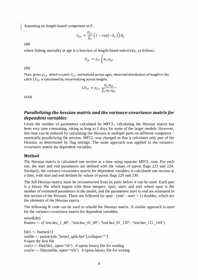
Assuming no length-based component in F,

𝐶𝑓𝑗𝑡 =𝐹𝑓𝑗𝑡

𝑍𝑗𝑡 1 − 𝑒𝑥𝑝 −𝑍𝑗𝑡 𝑁𝑗𝑡

(A8)

where fishing mortality at age is a function of length-based selectivity, as follows.

𝐹𝑓𝑗𝑡 = 𝜆𝑓𝑡 𝛼𝑓𝑖𝑞𝑖𝑗𝑡𝑖

(A9)

Then, given 𝑝𝑓𝑗𝑡 which is catch 𝐶𝑓𝑗𝑡 normalized across ages, observed distribution of length in the

catch 𝐿𝐹𝑓𝑖𝑡 is calculated by renormalizing across lengths

𝐿𝐹𝑓𝑖𝑡 = 𝑝𝑓𝑗𝑡 𝛼𝑓𝑖𝑞𝑖𝑗𝑡

𝛼𝑓𝑖𝑞𝑖𝑗𝑡𝑖

(A10)

Parallelizing the hessian matrix and the variance-covariance matrix for dependent variables Given the number of parameters calculated by MFCL, calculating the Hessian matrix has

been very time consuming, taking as long as 2 days for some of the larger models. However,

this time can be reduced by calculating the Hessian in multiple parts on different computers –

essentially parallelizing the process. MFCL was changed so that it calculates only part of the

Hessian, as determined by flag settings. The same approach was applied to the variance-

covariance matrix for dependent variables.

Method

The Hessian matrix is calculated one section at a time using separate MFCL runs. For each

run, the start and end parameters are defined with the values of parest flags 223 and 224.

Similarly, the variance-covariance matrix for dependent variables is calculated one section at

a time, with start and end defined by values of parest flags 229 and 230.

The full Hessian matrix must be reconstructed from its parts before it can be used. Each part

is a binary file which begins with three integers: npar, start, and end, where npar is the

number of estimated parameters in the model, and the parameters start to end are estimated in

this section of the Hessian. These are followed by npar . (end – start + 1) doubles, which are

the elements of the Hessian matrix.

The following R code can be used to rebuild the Hessian matrix. A similar approach is used

for the variance-covariance matrix for dependent variables.

setwd(dir)

fnames <- c("test.hes_1_40", “test.hes_41_80”, “test.hes_81_120”, “test.hes_121_160”)

file1 <- fnames[1]

outfile <- paste(c(dir,"lensel_split.hes"),collapse="")

# open the first file

con1r <- file(file1, open="rb") # opens binary file for reading

con2w <- file(outfile, open="wb") # opens binary file for writing

7

close(con2w)

con2w <- file(outfile, open="ab") # opens binary file for appending

# read the first file

size<- readBin(con1r, "integer", n = 3)

npar <- size[1]

nrows <- size[3] - size[2] + 1

a <- matrix(nrow=nrows,ncol=npar)

prow <- 0

writeBin(npar, con2w)

for (i in 1:nrows)

{

prow <- prow+1

a[i,] <- readBin(con1r, "double", n = npar)

writeBin(a[i,],con2w)

}

close(con1r)

for (ff in 2:length(fnames))

{

con <- file(fnames[ff], open="rb") # opens binary file for reading

s2 <-readBin(con, "integer", n = 3)

a <- matrix(nrow=nrows,ncol=npar)

for (i in 1:min(c(nrows,npar-nrows*(ff-1))))

{

prow <- prow+1

tmp <- readBin(con, "double", n = npar)

a[i,] <- tmp

writeBin(a[i,],con2w)

}

close(con)

}

close(con2w)

Projection with a mixture of catch and effort Multifan-CL can predict future population levels and catches by projecting the population

forward, using either expected catch or expected effort to constrain the catch removed.

However, it has not previously been able to project using a mixture of catch and effort. Some

proposed management measures place catch limits on some fisheries and effort limits on

others, and MFCL has been changed in order to model these scenarios.

Time-varying effort deviate weights (sd on CPUE) MFCL‟s approach for modeling uncertainty in CPUE has been enhanced to include an option

to weight CPUE temporally according to values input in the frq file. This will permit the

inclusion of variances estimated during CPUE standardization.

8

The data file is changed to version 6, and an additional column is added, to the right of the

effort column.

This effort weight column is multiplied by the standard effort weight for that fishery, which is

entered as fish flag 13, as before.

No associated changes were required to the output formats.

Other enhancements and bug fixes

Missing effort problem Missing catch or missing effort information is indicated in MFCL by the code -1 in the .frq

file. Where the standard catch equation is being used, MFCL estimates missing catch values

from the effort, and does not produce a catch deviate. When effort is missing and the standard

catch equation is being used, MFCL has until now interpolated a value from other effort

values for that fishery, and down-weighted the penalty due to the effort deviate. However,

problems have arisen in cases where the effort deviate has been so large as to hit the

boundary. With the effort deviate at the boundary, the model could not estimate the

appropriate catch, resulting in a large catch deviate. Large catch deviates reduce the model fit

and so can significantly bias the parameter estimates. This was a serious problem for the 2008

albacore assessment.

MFCL was changed to resolve this problem. For observations with catch but missing effort,

the catch conditioned approach is applied. This means that the catch is assumed to be known,

and no effort deviate is estimated. As a result, the correct catch is taken out, but no catch

deviate or effort deviate penalties are added to the likelihood.

Impact analysis The „no fishing‟ analysis was not working when steepness (e.g. the stock recruitment

relationship) was taken into account, i.e. with age flag 171 turned on. An error was reported

during impact analysis, and recruitment values for all but t=1 were set to low values. As a

result, impact analyses had to be run with the flag switched off, so they did not adjust

recruitment for the higher spawning biomass of unfished populations.

The reason for this bug was discovered and the code changed, so the stock recruitment

relationship can now be taken into account.

Application of length-based selectivity Both the standard and the length-based selectivity models were applied to the albacore and

bigeye tuna data sets, as used in the 2008 assessments (Hoyle et al. 2008; Langley et al.

2008).

9

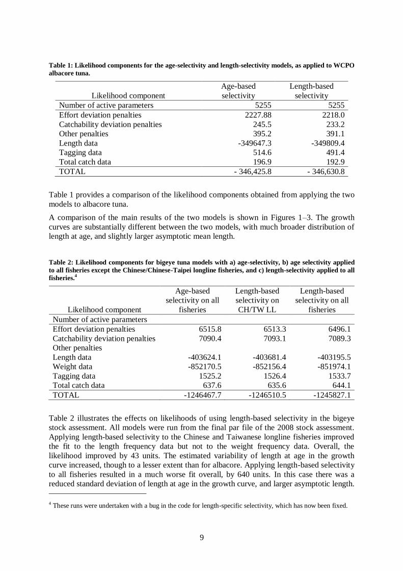
Table 1: Likelihood components for the age-selectivity and length-selectivity models, as applied to WCPO

albacore tuna.

Likelihood component

Age-based

selectivity

Length-based

selectivity

Number of active parameters 5255 5255

Effort deviation penalties 2227.88 2218.0

Catchability deviation penalties 245.5 233.2

Other penalties 395.2 391.1

Length data -349647.3 -349809.4

Tagging data 514.6 491.4

Total catch data 196.9 192.9

TOTAL - 346,425.8 - 346,630.8

Table 1 provides a comparison of the likelihood components obtained from applying the two

models to albacore tuna.

A comparison of the main results of the two models is shown in Figures 1–3. The growth

curves are substantially different between the two models, with much broader distribution of

length at age, and slightly larger asymptotic mean length.

Table 2: Likelihood components for bigeye tuna models with a) age-selectivity, b) age selectivity applied

to all fisheries except the Chinese/Chinese-Taipei longline fisheries, and c) length-selectivity applied to all

fisheries.4

Likelihood component

Age-based

selectivity on all

fisheries

Length-based

selectivity on

CH/TW LL

Length-based

selectivity on all

fisheries

Number of active parameters

Effort deviation penalties 6515.8 6513.3 6496.1

Catchability deviation penalties 7090.4 7093.1 7089.3

Other penalties

Length data -403624.1 -403681.4 -403195.5

Weight data -852170.5 -852156.4 -851974.1

Tagging data 1525.2 1526.4 1533.7

Total catch data 637.6 635.6 644.1

TOTAL -1246467.7 -1246510.5 -1245827.1

Table 2 illustrates the effects on likelihoods of using length-based selectivity in the bigeye

stock assessment. All models were run from the final par file of the 2008 stock assessment.

Applying length-based selectivity to the Chinese and Taiwanese longline fisheries improved

the fit to the length frequency data but not to the weight frequency data. Overall, the

likelihood improved by 43 units. The estimated variability of length at age in the growth

curve increased, though to a lesser extent than for albacore. Applying length-based selectivity

to all fisheries resulted in a much worse fit overall, by 640 units. In this case there was a

reduced standard deviation of length at age in the growth curve, and larger asymptotic length.

4 These runs were undertaken with a bug in the code for length-specific selectivity, which has now been fixed.

10

These were unexpected results that require further analysis. A better solution may be found

by starting from the bet.ini file, rather than from the converged age-based selectivity fit.

Future work The future work plan for MFCL is outlined in Table 3.

Discussion A number of changes have been made to MFCL during 2008-2009. Although a number of

model shortcomings were found and rectified, they did not change the management

implications of model results in any significant way. However, considerable further work is

required to comprehensively test all changes to the model, and to update all the changes to

the manual. One very important task for 2009-2010 will be to develop an automated model

testing routine.

The two other major development areas for 2008-2009 will be to increase the flexibility of

tag modeling, as the Pacific Tuna Tagging Program results become available, and to improve

model diagnostics, so that problems in model fit can be identified and resolved.

We also see a strong need to develop „extension‟ tools that will allow managers and

stakeholders to gain a better understanding of the model results, and of the results of

management options analyses. We see this requiring the development of a purpose-built

software tool, which will work as an add-in to MFCL.

11

Figure 1: Growth curves for south Pacific albacore estimated using age-based and length-based

selectivity. The value of K is fixed, but the model estimates lengths at age 1 and 20, and the standard

deviation of length at age.

12

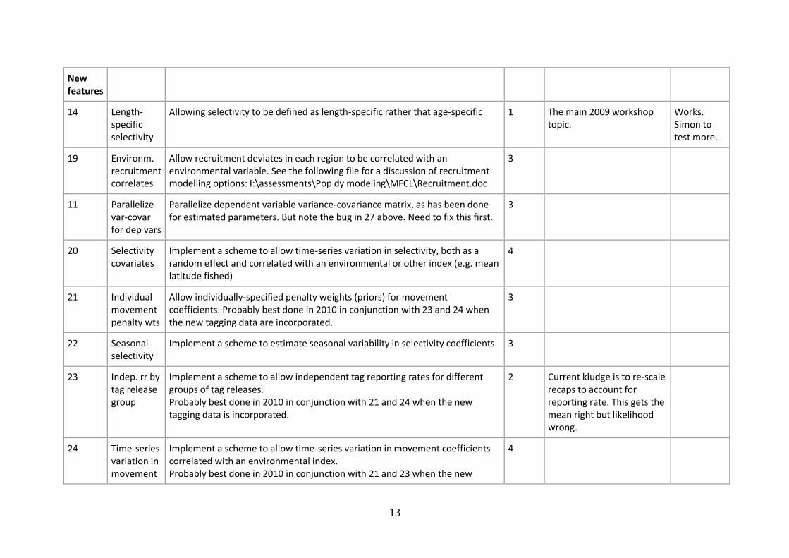
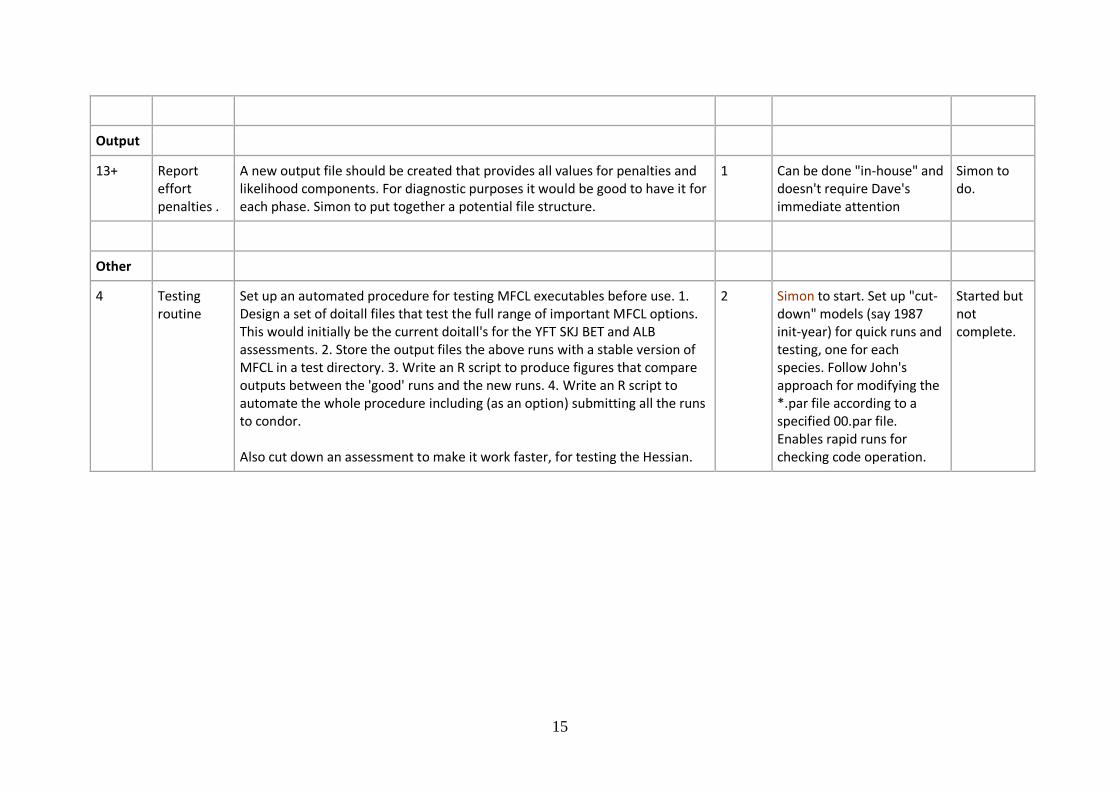
Table 3: 2008-2009 work plan for MFCL, including work completed and suggested future enhancements.

ID Item Description / Comment Priority Comments Status

Bugs

No fishing analysis

The no-fishing analysis does not work if steepness (e.g. the SRR) is taken into account. When af_171 is turned on, an error is reported during impact analysis, and recruitments for all but t=1 are set to low values. See the following URL for example with attached files.

1 Bug report Nov 20. See emails.

Works. Simon to do more testing

5 Catches in projections

Previously there have been problems with the predicted catches (longline) from the projection period. Unsure if this has been fixed or if there are other catch / projection problems.

1 Issue related to running out of fish may be outstanding. John to check current status.

12 & 27 Hessian problems

1. Errors in xinit.rpt. Has this been fixed already? 2. Currently doesn't seem to put Hessian back together in a usable way when

it is parallelised using Condor. Simon to work on with Dave 3. Dependent variable Hessian needs to be parallelized too. Also needs

pruning. Simon to make a list and distribute.

1 An example model should be developed for Dave to work with.

1. Fixed 2. Works 3. In

progress

15 MSY in projection period

Problem with estimating MSY and related in the projection period. Has this been fixed already?

1 Fixed Works

28 Missing effort

When effort is missing, an effort value is interpolated between actual effort estimates in the time series. Sometimes this value is such an outlier (given the catch) that effort devs hit the boundary. Also, multiple missing efforts can result in bias. Suggestions include calculating an effort value by solving the equations for the total catch (as in catch conditioned model).

1 Done. Works. Simon to do more testing

13

New features

14 Length-specific selectivity

Allowing selectivity to be defined as length-specific rather that age-specific 1 The main 2009 workshop topic.

Works. Simon to test more.

19 Environm. recruitment correlates

Allow recruitment deviates in each region to be correlated with an environmental variable. See the following file for a discussion of recruitment modelling options: I:\assessments\Pop dy modeling\MFCL\Recruitment.doc

3

11 Parallelize var-covar for dep vars

Parallelize dependent variable variance-covariance matrix, as has been done for estimated parameters. But note the bug in 27 above. Need to fix this first.

3

20 Selectivity covariates

Implement a scheme to allow time-series variation in selectivity, both as a random effect and correlated with an environmental or other index (e.g. mean latitude fished)

4

21 Individual movement penalty wts

Allow individually-specified penalty weights (priors) for movement coefficients. Probably best done in 2010 in conjunction with 23 and 24 when the new tagging data are incorporated.

3

22 Seasonal selectivity

Implement a scheme to estimate seasonal variability in selectivity coefficients 3

23 Indep. rr by tag release group

Implement a scheme to allow independent tag reporting rates for different groups of tag releases. Probably best done in 2010 in conjunction with 21 and 24 when the new tagging data is incorporated.

2 Current kludge is to re-scale recaps to account for reporting rate. This gets the mean right but likelihood wrong.

24 Time-series variation in movement

Implement a scheme to allow time-series variation in movement coefficients correlated with an environmental index. Probably best done in 2010 in conjunction with 21 and 23 when the new

4

14

coefficients tagging data is incorporated.

25 Uncertainty in projected biomass

Implement a scheme to compute uncertainty in projected population biomass by propagating uncertainty in recruitment and effort deviations in the projection period. This must be done in such a way that the parameter estimates and likelihoods for the time period supported by data are unaffected (e.g. Maunder, Harley, and Hampton paper in ICESJMS).

2 Dave had previously drafted notes on how to do this correctly - need to dig these up.

26 Estimate biological parameters at length

Maturity, fecundity, spawning fraction are typically length-specific properties (at least the data on them is) and so they are converted to age based on the initial growth curve. As soon as a growth curve is estimated there is an inconsistency.

3

Projection-related analysis capabilities

Being able to do projections based on F (all fisheries) and for effort and catch for different fisheries (e.g. evaluate effort based limits for purse seine and catch based limits for longline). Also to keep consistent with the yield-based approaches we need to be able to us an average catchability for the future (if we can’t already). Also see 25 above.

1 Nick to document notes from FFA Bio-economic workshop projections (with Adam). Use YFT projections as an example model for generating output. Run tests for either effort- or catch-specified projections.

In progress. Nick follow up with Dave.

Yield-related analysis capabilities

Estimate indicative yields by fishery for both MSY and Equilibrium yield. Also, the current MSY calculations estimate a single F-scalar across all fisheries. It would be useful to estimate region-specific scalars. Anything more than that would lead to estimation difficulties.

2 Region-specific yield calculations are already an option in MFCL. (See section in code called "Daves_folly")

Hyper-stability

Implement fishery-specific hyperstability, as a relationship between vulnerable biomass and catchability

3

Projections Add projection period into par file automatically. Could be done in R. 1. Write read.par & write.par. 2. ID all fields in par obj. 3. Write functions to modify par object

3 New task13/1 Drafted read.par +write.par

15

Output

13+ Report effort penalties .

A new output file should be created that provides all values for penalties and likelihood components. For diagnostic purposes it would be good to have it for each phase. Simon to put together a potential file structure.

1 Can be done "in-house" and doesn't require Dave's immediate attention

Simon to do.

Other

4 Testing routine

Set up an automated procedure for testing MFCL executables before use. 1. Design a set of doitall files that test the full range of important MFCL options. This would initially be the current doitall's for the YFT SKJ BET and ALB assessments. 2. Store the output files the above runs with a stable version of MFCL in a test directory. 3. Write an R script to produce figures that compare outputs between the 'good' runs and the new runs. 4. Write an R script to automate the whole procedure including (as an option) submitting all the runs to condor. Also cut down an assessment to make it work faster, for testing the Hessian.

2 Simon to start. Set up "cut-down" models (say 1987 init-year) for quick runs and testing, one for each species. Follow John's approach for modifying the *.par file according to a specified 00.par file. Enables rapid runs for checking code operation.

Started but not complete.

16

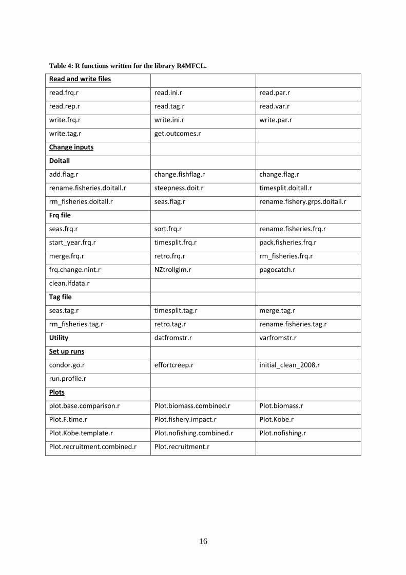
Table 4: R functions written for the library R4MFCL.

Read and write files

read.frq.r read.ini.r read.par.r

read.rep.r read.tag.r read.var.r

write.frq.r write.ini.r write.par.r

write.tag.r get.outcomes.r

Change inputs

Doitall

add.flag.r change.fishflag.r change.flag.r

rename.fisheries.doitall.r steepness.doit.r timesplit.doitall.r

rm_fisheries.doitall.r seas.flag.r rename.fishery.grps.doitall.r

Frq file

seas.frq.r sort.frq.r rename.fisheries.frq.r

start_year.frq.r timesplit.frq.r pack.fisheries.frq.r

merge.frq.r retro.frq.r rm_fisheries.frq.r

frq.change.nint.r NZtrollglm.r pagocatch.r

clean.lfdata.r

Tag file

seas.tag.r timesplit.tag.r merge.tag.r

rm_fisheries.tag.r retro.tag.r rename.fisheries.tag.r

Utility datfromstr.r varfromstr.r

Set up runs

condor.go.r effortcreep.r initial_clean_2008.r

run.profile.r

Plots

plot.base.comparison.r Plot.biomass.combined.r Plot.biomass.r

Plot.F.time.r Plot.fishery.impact.r Plot.Kobe.r

Plot.Kobe.template.r Plot.nofishing.combined.r Plot.nofishing.r

Plot.recruitment.combined.r Plot.recruitment.r

17

Reference List

1. Hoyle, S. D. and Langley, A. D. 2007. Comparison of South Pacific albacore stock assessments

using MULTIFAN-CL and STOCK SYNTHESIS 2. Secretariat of the Pacific Community No.

WCPFC-SC3-ME SWG/WP-6.

2. Hoyle, Simon D., Langley, Adam D., and Hampton, W. J. 2008. Stock assessment of Albacore tuna

in the south Pacific Ocean. Secretariat of the Pacific Community No. WCPFC-SC4-2008/ SA-WP-8.

3. Langley, A. D., Hampton, J., Kleiber, P. M., and Hoyle, S. D. 2007. Stock assessment of yellowfin

tuna in the western and central Pacific Ocean, including an analysis of management options.

Secretariat of the Pacific Community No. WCPFC-SC3, SA WP-1.

4. Langley, A. D., Hampton, W. J., Kleiber, P. M., and Hoyle, S. D. 2008. Stock assessment of bigeye

tuna in the western and central Pacific ocean, including an analysis of management options.

Secretariat of the Pacific Community No. WCPFC-SC4-2008/SA-WP-1 .

5. Methot, Richard D. 2007. User Manual for the Integrated Analysis Program Stock Synthesis 2

(SS2): Model Version 2.00c.