Scientific Computing II

Overview

Michael BaderTechnical University of Munich

Summer 2017

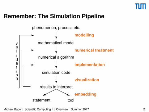
Remember: The Simulation Pipeline

phenomenon, process etc.

mathematical model?

modelling

numerical algorithm?

numerical treatment

simulation code?

implementation

results to interpret?

visualization

�����HHHHj embedding

statement tool

-

-

-

validation

Michael Bader | Scientific Computing II | Overview | Summer 2017 2

Topic #1: Solving Systems of Linear Equations

Focussing on• large systems: 106–109 unknowns• sparse systems: typically only O(N) non-zeros in the system matrix

(N unknowns)• systems resulting from the discretization of PDEs

Topics• relaxation methods (as smoothers)• multigrid methods• Conjugate Gradient methods• preconditioning

Michael Bader | Scientific Computing II | Overview | Summer 2017 3

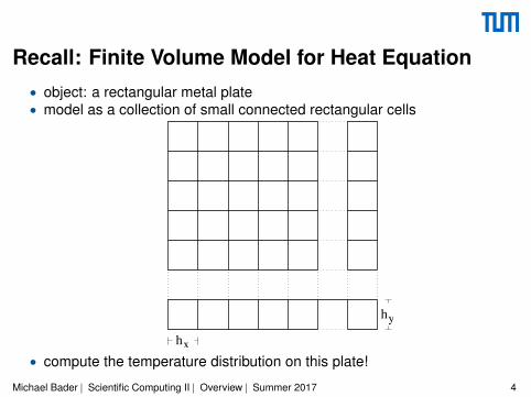
Recall: Finite Volume Model for Heat Equation• object: a rectangular metal plate• model as a collection of small connected rectangular cells

hx

hy

• compute the temperature distribution on this plate!

Michael Bader | Scientific Computing II | Overview | Summer 2017 4

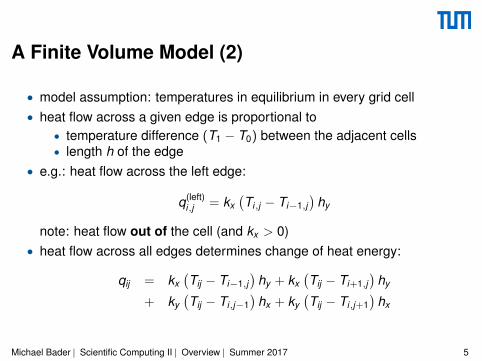
A Finite Volume Model (2)

• model assumption: temperatures in equilibrium in every grid cell• heat flow across a given edge is proportional to

• temperature difference (T1 − T0) between the adjacent cells• length h of the edge

• e.g.: heat flow across the left edge:

q(left)i,j = kx

(Ti,j − Ti−1,j

)hy

note: heat flow out of the cell (and kx > 0)• heat flow across all edges determines change of heat energy:

qij = kx(Tij − Ti−1,j

)hy + kx

(Tij − Ti+1,j

)hy

+ ky(Tij − Ti,j−1

)hx + ky

(Tij − Ti,j+1

)hx

Michael Bader | Scientific Computing II | Overview | Summer 2017 5

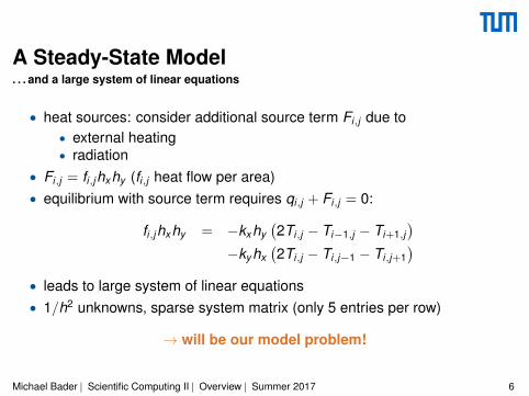
A Steady-State Model. . . and a large system of linear equations

• heat sources: consider additional source term Fi,j due to• external heating• radiation

• Fi,j = fi,jhxhy (fi,j heat flow per area)• equilibrium with source term requires qi,j + Fi,j = 0:

fi,jhxhy = −kxhy(2Ti,j − Ti−1,j − Ti+1,j

)−ky hx

(2Ti,j − Ti,j−1 − Ti,j+1

)• leads to large system of linear equations• 1/h2 unknowns, sparse system matrix (only 5 entries per row)

→ will be our model problem!

Michael Bader | Scientific Computing II | Overview | Summer 2017 6

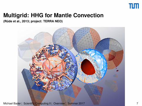
Multigrid: HHG for Mantle Convection(Rude et al., 2013; project: TERRA NEO)

Michael Bader | Scientific Computing II | Overview | Summer 2017 7

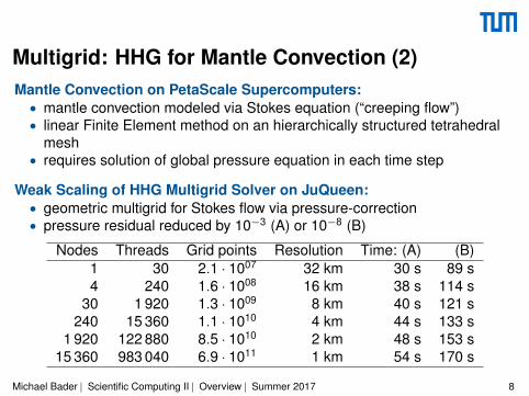
Multigrid: HHG for Mantle Convection (2)Mantle Convection on PetaScale Supercomputers:

• mantle convection modeled via Stokes equation (“creeping flow”)• linear Finite Element method on an hierarchically structured tetrahedral

mesh• requires solution of global pressure equation in each time step

Weak Scaling of HHG Multigrid Solver on JuQueen:• geometric multigrid for Stokes flow via pressure-correction• pressure residual reduced by 10−3 (A) or 10−8 (B)

Nodes Threads Grid points Resolution Time: (A) (B)1 30 2.1 · 1007 32 km 30 s 89 s4 240 1.6 · 1008 16 km 38 s 114 s

30 1 920 1.3 · 1009 8 km 40 s 121 s240 15 360 1.1 · 1010 4 km 44 s 133 s

1 920 122 880 8.5 · 1010 2 km 48 s 153 s15 360 983 040 6.9 · 1011 1 km 54 s 170 s

Michael Bader | Scientific Computing II | Overview | Summer 2017 8

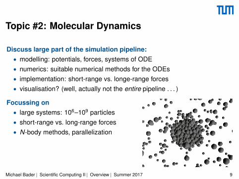
Topic #2: Molecular Dynamics

Discuss large part of the simulation pipeline:• modelling: potentials, forces, systems of ODE• numerics: suitable numerical methods for the ODEs• implementation: short-range vs. longe-range forces• visualisation? (well, actually not the entire pipeline . . . )

Focussing on• large systems: 106–109 particles• short-range vs. long-range forces• N-body methods, parallelization

Michael Bader | Scientific Computing II | Overview | Summer 2017 9

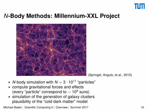
N-Body Methods: Millennium-XXL Project

(Springel, Angulo, et al., 2010)

• N-body simulation with N = 3 · 1011 “particles”• compute gravitational forces and effects

(every “particle” correspond to ∼ 109 suns)• simulation of the generation of galaxy clusters

plausibility of the “cold dark matter” modelMichael Bader | Scientific Computing II | Overview | Summer 2017 10

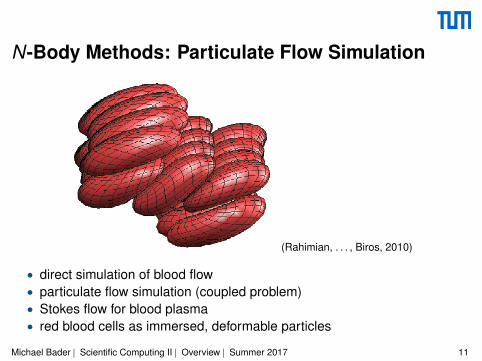
N-Body Methods: Particulate Flow Simulation

(Rahimian, . . . , Biros, 2010)

• direct simulation of blood flow• particulate flow simulation (coupled problem)• Stokes flow for blood plasma• red blood cells as immersed, deformable particles

Michael Bader | Scientific Computing II | Overview | Summer 2017 11

Organisation

Michael Bader | Scientific Computing II | Overview | Summer 2017 12

Exams, ECTS, Modules

ECTS, Modules• 5 ECTS (2+2 lectures/tutorials per week)• CSE: compulsory course• Biomed. Computing/Computer Science:

elective/Master catalogue• others?

Tutorials:• tutor: Carsten Uphoff• time and day: Tue, 10-12, MI 02.07.023

Exam:• written exam at end of semester• based on exercises presented in the tutorials

Michael Bader | Scientific Computing II | Overview | Summer 2017 13

Lecture Slides: Color Code for Headers

Black Headers:• for all slides with regular topics

Green Headers:• summarized details: will be explained in the lecture, but usually not as an

explicit slide; “green” slides will only appear in the handout versions

Red Headers:• advanced topics or outlook: will not be part of the exam topics

Michael Bader | Scientific Computing II | Overview | Summer 2017 14