Embed Size (px)
Citation preview
SciPyTutorial DocumentationRelease 0.0.1
VG
January 31, 2011

CONTENTS
1 Basics 11.1 A Dialog on Python for Scientific Computing . . . . . . . . . . . . . . . . . . . . . . . . . . . . . . 11.2 Introduction . . . . . . . . . . . . . . . . . . . . . . . . . . . . . . . . . . . . . . . . . . . . . . . 21.3 Installation tips . . . . . . . . . . . . . . . . . . . . . . . . . . . . . . . . . . . . . . . . . . . . . . 31.4 First steps in Python . . . . . . . . . . . . . . . . . . . . . . . . . . . . . . . . . . . . . . . . . . . 51.5 Basic Tutorial . . . . . . . . . . . . . . . . . . . . . . . . . . . . . . . . . . . . . . . . . . . . . . . 371.6 IPython tips . . . . . . . . . . . . . . . . . . . . . . . . . . . . . . . . . . . . . . . . . . . . . . . . 501.7 Matplotlib tips . . . . . . . . . . . . . . . . . . . . . . . . . . . . . . . . . . . . . . . . . . . . . . 561.8 Mayavi2 tips . . . . . . . . . . . . . . . . . . . . . . . . . . . . . . . . . . . . . . . . . . . . . . . 591.9 Other noteworthy plot commands . . . . . . . . . . . . . . . . . . . . . . . . . . . . . . . . . . . . 641.10 Examples . . . . . . . . . . . . . . . . . . . . . . . . . . . . . . . . . . . . . . . . . . . . . . . . . 651.11 Useful links . . . . . . . . . . . . . . . . . . . . . . . . . . . . . . . . . . . . . . . . . . . . . . . . 741.12 Installing python packages . . . . . . . . . . . . . . . . . . . . . . . . . . . . . . . . . . . . . . . . 75
2 Advanced Stuff 772.1 Optimization of Python Code . . . . . . . . . . . . . . . . . . . . . . . . . . . . . . . . . . . . . . 772.2 Timing Your Code . . . . . . . . . . . . . . . . . . . . . . . . . . . . . . . . . . . . . . . . . . . . 782.3 Gluing Stand-Alone Applications . . . . . . . . . . . . . . . . . . . . . . . . . . . . . . . . . . . . 822.4 Symbolical calculations . . . . . . . . . . . . . . . . . . . . . . . . . . . . . . . . . . . . . . . . . 862.5 Making of: animations . . . . . . . . . . . . . . . . . . . . . . . . . . . . . . . . . . . . . . . . . . 882.6 Input / Output of numerical data . . . . . . . . . . . . . . . . . . . . . . . . . . . . . . . . . . . . . 912.7 Combining Python with Fortran, C and C++ . . . . . . . . . . . . . . . . . . . . . . . . . . . . . . 94
3 Indices and tables 99
Index 101
i

ii
CHAPTER
ONE
BASICS
Contents:
1.1 A Dialog on Python for Scientific Computing
Why should I learn Python?
If you consider the possibility that you will work in a different domain thanpure mathematics, then there is a good chance that you will need it at a givenmoment of your career.
It is used in the industry?
Yes, it is used in many companies and by research institutions that usecomputers as an instrument.
Why? I thought there is Java and C++ and so on...
With Python you can develop and prototype your products much more quickly. Ifneeded, parts of your production code can later be migrated toC/C++/Fortran/Java or whatever.
Whatever?
Yes. One of the qualities that qualified Python to large industrialapplication is its affinity to many programming languages. This makes it easyto embed applications in both directions.
Aha, so you glue together tools.
Yes, Python is a perfect scripting language, but here I meant that you canreally mix programming languages in an easy and consistent way.
What is scripting?
Scripting is a way to let very different applications play together toachieve your aim. This is another quality that makes Python attractive for theindustry.
What about research and scientific work?
As a researcher, you would like to know quite soon if your idea makessense. You would like to run simulations as soon as possible, so you wantquickly a correct prototype and not a prototype that runs quickly...
1
SciPyTutorial Documentation, Release 0.0.1
But that was one of the attractions of matlab, so what’s new?
If the idea works and the code gives you correct results, but you want it moreefficiently or you want to scope it to other codes or professional visualizationtools, then it is much simpler to migrate parts of python code than to re-writethe code from scratch, as usually happens with matlab projects.
I see. So with python I can glue applications together and can migrate critical numerical parts to C/Fortran. But if I donot need to? Isn’t matlab enough?
Enough? This is a good word!It depends. Earlier I used to say: if you are satisfied with matlab and you donot feel you need something more, then stay with matlab.
And now?
Now I would be more careful. I noticed that people prefer to use what theylearned first than to learn something new. This means that when people get adifficult new problem, they make great efforts to solve it with the tools theyknow better. This gives complicated solutions after great efforts, wheresimple rush solutions were possible with new knowledge. You have to hit thewall, and the hit must really hurt, in order to be really willing to learnsomething new. I am sure that people are more efficient and more likely toobtain good and rush solutions to hard problems if they learn python (andscientific tools) first.
You mean that you can solve more difficult problems with python than with matlab?
I mean that with python et al you have better chances, especially for large projects.
Why should we learn or use python for teaching numerical methods? Isn’t it much too complex? Isn’t it simpler touse matlab for this aim?
When you start from zero, you need the same effort to learn matlab and Python.
matlab is a very good software. It has also its price, which is very high,if you leave the university. Most of our students will not remain in auniversity, so working in a small company would be a clear handicap forour alumni.
matlab is a good software because it was developed over several years undervery strict guidelines. Hence, it is more stable than the on-going developmentversions of python et al.
For the very same reasons that make matlab very stable, matlab is very rigid.Having to cope with the main ideas of 1970-80 makes improvements very hardto realize. Object-orientation is the best example in this sense. It had tobe introduced in order to make matlab survive, but apart from its marketingeffect, it is useless, since it rather hampers than facilitates developmentand code-reuse. Respecting old guidelines makes matlab strong, but rigid andrather past-oriented. On the contrary, our students will live in the future,let us give them a chance to make a better world!
1.2 Introduction
The aim of these pages is to provide enough information in order to help students to start using python’s tools forcomputational science, numerical methods and implementation of numerical algorithms.
2 Chapter 1. Basics
SciPyTutorial Documentation, Release 0.0.1
Python is not a Matlab clone, but a very flexible and very powerful (be aware!) high-level programming language.Still, it is so simple to use, that we’ll learn it by doing our own job... We focus on scientific computing now, butyou might use it for very different tasks, from controlling your experimental machines, by making high-performancevisualizations, to sorting your mp3’s on your mobile phone.
While coming with ‘batteries included’ python is only a small kernel that should be completed by modules specializedfor your aims.
We’ll use the following python modules:
• numpy
• scipy
• matplotlib
• ipython
• mayavi2
Please, consult Installation tips before retrieving these modules.
Work flow Personally, I use my preferred editor (emacs) and the improved interactive environ-ment IPython for the design and test of the scripts; the actual tutorial assumes this working style.You might consider also one of the following alternatives to (editor+ipython):
• spyder (similar to the Matlab-environment)
• eric (similar to the Eclipse-environment)
The editor scite comes with the pythonxy package for Windows and is well suited for writing python files.
1.3 Installation tips
1.3.1 All at once if you are allowed
The main difficulty in the bottom-up installation is to discover the correct dependences of the modules. You can avoidthis difficulty by using packages:
• Linux package manager: look for enthought distribution (e.g. present on Mandriva Free 2010.0); if this is notpresent then look for mayavi2 and scipy, then for ipython, matplotlib and nose (for having testing enabled)
• On Windows 32 bits you can use pyhtonxy that includes apart the main scientific modules and spyder and scite,too.
• The Enthought Python Distribution (EPD) is available for several operation systems (including Windows andMacOS) free of charge for academic use (it requires registration).
In case of difficulties or special wishes, consult the web pages of scipy.
A basic installation (without spyder) is available on the computers for the students slab.
This tutorial was tested on fedora core 13 machines of D-MATH and slab which have Python 2.6.4. as well as on aWinXP-machine with Python(x,y)-2.6.5.3.
1.3.2 Installation of the Spyder IDE as non-root on linux
A short description on how to install the Spyder IDE as non-root on Linux, useful for instance on one of the computersslab*.ethz.ch.
The Spyder IDE is available for download at http://code.google.com/p/spyderlib/.
1.3. Installation tips 3
SciPyTutorial Documentation, Release 0.0.1
Prerequisites
The program needs the following dependencies which are grouped into required and extension packages.
• Dependencies (required):
– Python 2.x (x>=5)
– PyQt4 4.x (x>=3 ; recommended x>=4)
– QScintilla2 2.x (x>=1) (PyQt4 extension)
• Dependencies (optional):
– pylint (code analysis)
– numpy (N-dimensional arrays)
– scipy (signal/image processing)
– matplotlib (2D plotting)
Of course the last three optional dependencies are important and not really optional for us. However, these packagesare already installed on these computers.
Installation process
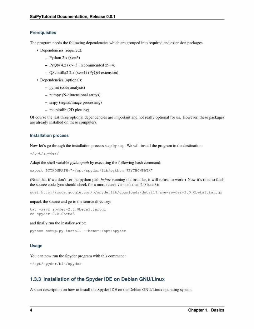
Now let’s go through the installation process step by step. We will install the program to the destination:
~/opt/spyder/
Adapt the shell variable pythonpath by executing the following bash command:
export PYTHONPATH="~/opt/spyder/lib/python:$PYTHONPATH"
(Note that if we don’t set the python path before running the installer, it will refuse to work.) Now it’s time to fetchthe source code (you should check for a more recent versions than 2.0 beta 3):
wget http://code.google.com/p/spyderlib/downloads/detail?name=spyder-2.0.0beta3.tar.gz
unpack the source and go to the source directory:
tar -xzvf spyder-2.0.0beta3.tar.gzcd spyder-2.0.0beta3
and finally run the installer script:
python setup.py install --home=~/opt/spyder
Usage
You can now run the Spyder program with this command:
~/opt/spyder/bin/spyder
1.3.3 Installation of the Spyder IDE on Debian GNU/Linux
A short description on how to install the Spyder IDE on the Debian GNU/Linux operating system.
4 Chapter 1. Basics
SciPyTutorial Documentation, Release 0.0.1
The spyder IDE
The Spyder python IDE is contained in the official package repositories of the Debian GNU/Linux distribution. Thusinstalling the software is rather trivial. You just have to tell the package manager to install the package and he willautomatically pull and install all required dependent packages too. (This includes other python packages but also morelow level stuff like the BLAS routines if necessary.)
The shell command doing all the magic is as simple as:
apt-get install spyder
(You can use any other package manager frontend like aptitude or synaptic instead of apt-get.) This willwork on Ubuntu Linux too, the most recent version Maverick Meerkat ships with the spyder package. (Butmaybe it’s not installed by default.)
Other python packages on Debian
In the following we list some more Debian packages related to python and the tools we are going to use in this tutorial.Many of these will get installed as dependencies of the spyder package already, others are optional. You may want totry some of them nevertheless.
• ipython: enhanced interactive Python shell
• mayavi2: A scientific visualization package for 2-D and 3-D data
• winpdb: Platform independent Python debugger
• spe: Stani’s Python Editor (Another python IDE)
• pylint: python code static checker and UML diagram generator
• pyflakes: passive checker of Python programs
• python-numpy: Numerical Python adds a fast array facility to the Python language
• python-numpy-doc: NumPy documentation
• python-scipy: scientific tools for Python
• python-symeig: Symmetrical eigenvalue routines for NumPy
• python-matplotlib: Python based plotting system in a style similar to Matlab
• python-sympy: Computer Algebra System (CAS) in Python
• python-imaging: Python Imaging Library
• python-mpmath: library for arbitrary-precision floating-point arithmetic
• python-enthoughtbase: Core packages for the Enthought Tool Suite
• python-epydoc: tool for documenting Python modules
• python-sphinx: tool for producing documentation for Python projects
1.4 First steps in Python
1.4.1 Fast-track Python
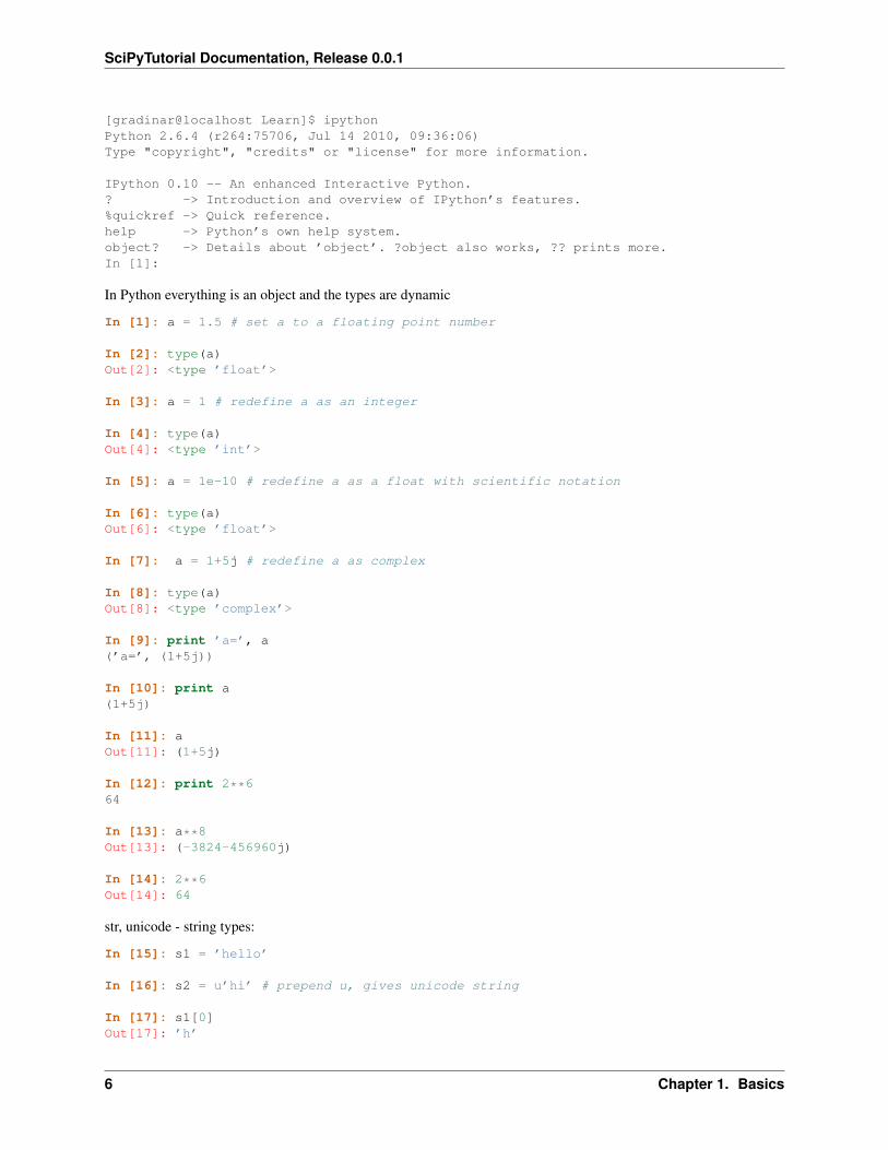
Start an IPython session
1.4. First steps in Python 5
SciPyTutorial Documentation, Release 0.0.1
[gradinar@localhost Learn]$ ipythonPython 2.6.4 (r264:75706, Jul 14 2010, 09:36:06)Type "copyright", "credits" or "license" for more information.
IPython 0.10 -- An enhanced Interactive Python.? -> Introduction and overview of IPython’s features.%quickref -> Quick reference.help -> Python’s own help system.object? -> Details about ’object’. ?object also works, ?? prints more.In [1]:
In Python everything is an object and the types are dynamic
In [1]: a = 1.5 # set a to a floating point number
In [2]: type(a)Out[2]: <type ’float’>
In [3]: a = 1 # redefine a as an integer
In [4]: type(a)Out[4]: <type ’int’>
In [5]: a = 1e-10 # redefine a as a float with scientific notation
In [6]: type(a)Out[6]: <type ’float’>
In [7]: a = 1+5j # redefine a as complex
In [8]: type(a)Out[8]: <type ’complex’>
In [9]: print ’a=’, a(’a=’, (1+5j))
In [10]: print a(1+5j)
In [11]: aOut[11]: (1+5j)
In [12]: print 2**664
In [13]: a**8Out[13]: (-3824-456960j)
In [14]: 2**6Out[14]: 64
str, unicode - string types:
In [15]: s1 = ’hello’
In [16]: s2 = u’hi’ # prepend u, gives unicode string
In [17]: s1[0]Out[17]: ’h’
6 Chapter 1. Basics
SciPyTutorial Documentation, Release 0.0.1
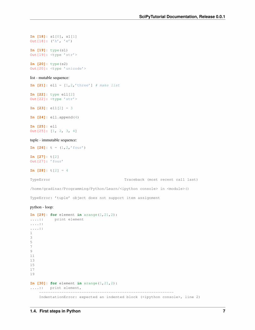
In [18]: s1[0], s1[1]Out[18]: (’h’, ’e’)
In [19]: type(s1)Out[19]: <type ’str’>
In [20]: type(s2)Out[20]: <type ’unicode’>
list - mutable sequence:
In [21]: ell = [1,2,’three’] # make list
In [22]: type ell[2]Out[22]: <type ’str’>
In [23]: ell[2] = 3
In [24]: ell.append(4)
In [25]: ellOut[25]: [1, 2, 3, 4]
tuple - immutable sequence:
In [26]: t = (1,2,’four’)
In [27]: t[2]Out[27]: ’four’
In [28]: t[2] = 4
TypeError Traceback (most recent call last)
/home/gradinar/Programming/Python/Learn/<ipython console> in <module>()
TypeError: ’tuple’ object does not support item assignment
python - loop:
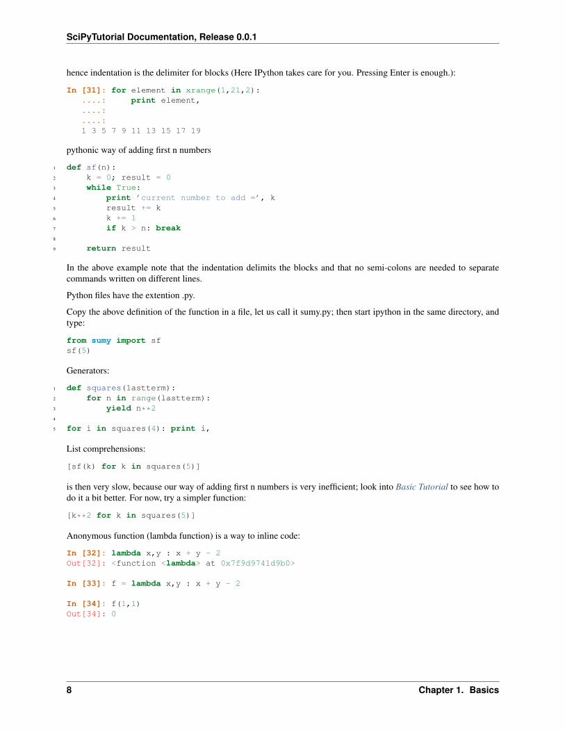
In [29]: for element in xrange(1,21,2):....:: print element....::....::135791113151719
In [30]: for element in xrange(1,21,2):....:: print element,
------------------------------------------------------------IndentationError: expected an indented block (<ipython console>, line 2)
1.4. First steps in Python 7
SciPyTutorial Documentation, Release 0.0.1
hence indentation is the delimiter for blocks (Here IPython takes care for you. Pressing Enter is enough.):
In [31]: for element in xrange(1,21,2):....: print element,....:....:1 3 5 7 9 11 13 15 17 19
pythonic way of adding first n numbers
1 def sf(n):2 k = 0; result = 03 while True:4 print ’current number to add =’, k5 result += k6 k += 17 if k > n: break8
9 return result
In the above example note that the indentation delimits the blocks and that no semi-colons are needed to separatecommands written on different lines.
Python files have the extention .py.
Copy the above definition of the function in a file, let us call it sumy.py; then start ipython in the same directory, andtype:
from sumy import sfsf(5)
Generators:
1 def squares(lastterm):2 for n in range(lastterm):3 yield n**24
5 for i in squares(4): print i,
List comprehensions:
[sf(k) for k in squares(5)]
is then very slow, because our way of adding first n numbers is very inefficient; look into Basic Tutorial to see how todo it a bit better. For now, try a simpler function:
[k**2 for k in squares(5)]
Anonymous function (lambda function) is a way to inline code:
In [32]: lambda x,y : x + y - 2Out[32]: <function <lambda> at 0x7f9d9741d9b0>
In [33]: f = lambda x,y : x + y - 2
In [34]: f(1,1)Out[34]: 0
8 Chapter 1. Basics
SciPyTutorial Documentation, Release 0.0.1
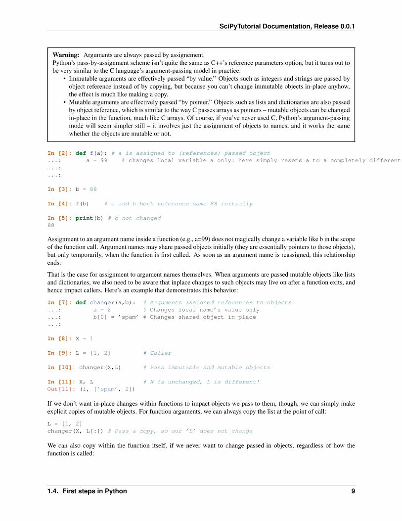
Warning: Arguments are always passed by assignement.Python’s pass-by-assignment scheme isn’t quite the same as C++’s reference parameters option, but it turns out tobe very similar to the C language’s argument-passing model in practice:
• Immutable arguments are effectively passed “by value.” Objects such as integers and strings are passed byobject reference instead of by copying, but because you can’t change immutable objects in-place anyhow,the effect is much like making a copy.
• Mutable arguments are effectively passed “by pointer.” Objects such as lists and dictionaries are also passedby object reference, which is similar to the way C passes arrays as pointers – mutable objects can be changedin-place in the function, much like C arrays. Of course, if you’ve never used C, Python’s argument-passingmode will seem simpler still – it involves just the assignment of objects to names, and it works the samewhether the objects are mutable or not.
In [2]: def f(a): # a is assigned to (references) passed object...: a = 99 # changes local variable a only: here simply resets a to a completely different object...:...:
In [3]: b = 88
In [4]: f(b) # a and b both reference same 88 initially
In [5]: print(b) # b not changed88
Assignment to an argument name inside a function (e.g., a=99) does not magically change a variable like b in the scopeof the function call. Argument names may share passed objects initially (they are essentially pointers to those objects),but only temporarily, when the function is first called. As soon as an argument name is reassigned, this relationshipends.
That is the case for assignment to argument names themselves. When arguments are passed mutable objects like listsand dictionaries, we also need to be aware that inplace changes to such objects may live on after a function exits, andhence impact callers. Here’s an example that demonstrates this behavior:
In [7]: def changer(a,b): # Arguments assigned references to objects...: a = 2 # Changes local name’s value only...: b[0] = ’spam’ # Changes shared object in-place...:
In [8]: X = 1
In [9]: L = [1, 2] # Caller
In [10]: changer(X,L) # Pass immutable and mutable objects
In [11]: X, L # X is unchanged, L is different!Out[11]: (1, [’spam’, 2])
If we don’t want in-place changes within functions to impact objects we pass to them, though, we can simply makeexplicit copies of mutable objects. For function arguments, we can always copy the list at the point of call:
L = [1, 2]changer(X, L[:]) # Pass a copy, so our ’L’ does not change
We can also copy within the function itself, if we never want to change passed-in objects, regardless of how thefunction is called:
1.4. First steps in Python 9
SciPyTutorial Documentation, Release 0.0.1
def changer(a, b):b = b[:] # Copy input list so we don’t impact callera = 2b[0] = ’spam’ # Changes our list copy only
Both of these copying schemes don’t stop the function from changing the object – they just prevent those changesfrom impacting the caller. To really prevent changes, we can always convert to immutable objects to force the issue.Tuples, for example, throw an exception when changes are attempted:
L = [1, 2]changer(X, tuple(L)) # Pass a tuple, so changes are errors
Elements of Python style are on Google Python Style Guide or PythonStyle.
Finally, the Zen of Python (hat you might find useful outside of Pyhton, too):
In [35]: import thisThe Zen of Python, by Tim Peters
Beautiful is better than ugly.Explicit is better than implicit.Simple is better than complex.Complex is better than complicated.Flat is better than nested.Sparse is better than dense.Readability counts.Special cases aren’t special enough to break the rules.Although practicality beats purity.Errors should never pass silently.Unless explicitly silenced.In the face of ambiguity, refuse the temptation to guess.There should be one-- and preferably only one --obvious way to do it.Although that way may not be obvious at first unless you’re Dutch.Now is better than never.Although never is often better than *right* now.If the implementation is hard to explain, it’s a bad idea.If the implementation is easy to explain, it may be a good idea.Namespaces are one honking great idea -- let’s do more of those!
1.4.2 More on the language
You can find more on Python in on-line tutorials and books. I enjoyed Learning Python by M. Lutz and Python in aNutshell by A. Martelli.
For your convenience, you might consult Raoul Bourquin’s syntheses of the python tutorial at python.org:
An Informal Introduction to Python
In the following examples, input and output are distinguished by the presence or absence of prompts (>>> and ...):to repeat the example, you must type everything after the prompt, when the prompt appears; lines that do not beginwith a prompt are output from the interpreter. Note that a secondary prompt on a line by itself in an example meansyou must type a blank line; this is used to end a multi-line command.
Many of the examples in this manual, even those entered at the interactive prompt, include comments. Comments inPython start with the hash character, #, and extend to the end of the physical line. A comment may appear at the startof a line or following whitespace or code, but not within a string literal. A hash character within a string literal is just
10 Chapter 1. Basics
SciPyTutorial Documentation, Release 0.0.1
a hash character. Since comments are to clarify code and are not interpreted by Python, they may be omitted whentyping in examples.
Some examples:
# this is the first commentSPAM = 1 # and this is the second comment
# ... and now a third!STRING = "# This is not a comment."
Using Python as a Calculator
Let’s try some simple Python commands. Start the interpreter and wait for the primary prompt, >>>. (It shouldn’ttake long.)
Numbers The interpreter acts as a simple calculator: you can type an expression at it and it will write the value.Expression syntax is straightforward: the operators +, -, * and / work just like in most other languages (for example,Pascal or C); parentheses can be used for grouping. For example:
>>> 2+24>>> # This is a comment... 2+24>>> 2+2 # and a comment on the same line as code4>>> (50-5*6)/45>>> # Integer division returns the floor:... 7/32>>> 7/-3-3
The equal sign (’=’) is used to assign a value to a variable. Afterwards, no result is displayed before the nextinteractive prompt:
>>> width = 20>>> height = 5*9>>> width * height900
A value can be assigned to several variables simultaneously:
>>> x = y = z = 0 # Zero x, y and z>>> x0>>> y0>>> z0
Variables must be “defined” (assigned a value) before they can be used, or an error will occur:
>>> # try to access an undefined variable... nTraceback (most recent call last):
1.4. First steps in Python 11
SciPyTutorial Documentation, Release 0.0.1
File "<stdin>", line 1, in <module>NameError: name ’n’ is not defined
There is full support for floating point; operators with mixed type operands convert the integer operand to floatingpoint:
>>> 3 * 3.75 / 1.57.5>>> 7.0 / 23.5
Complex numbers are also supported; imaginary numbers are written with a suffix of j or J. Complex numbers witha nonzero real component are written as (real+imagj), or can be created with the complex(real, imag)function.
>>> 1j * 1J(-1+0j)>>> 1j * complex(0,1)(-1+0j)>>> 3+1j*3(3+3j)>>> (3+1j)*3(9+3j)>>> (1+2j)/(1+1j)(1.5+0.5j)
Complex numbers are always represented as two floating point numbers, the real and imaginary part. To extract theseparts from a complex number z, use z.real and z.imag.
>>> a=1.5+0.5j>>> a.real1.5>>> a.imag0.5
The conversion functions to floating point and integer (float(), int() and long()) don’t work for complexnumbers — there is no one correct way to convert a complex number to a real number. Use abs(z) to get itsmagnitude (as a float) or z.real to get its real part.
>>> a=3.0+4.0j>>> float(a)Traceback (most recent call last):
File "<stdin>", line 1, in ?TypeError: can’t convert complex to float; use abs(z)>>> a.real3.0>>> a.imag4.0>>> abs(a) # sqrt(a.real**2 + a.imag**2)5.0
In interactive mode, the last printed expression is assigned to the variable _. This means that when you are usingPython as a desk calculator, it is somewhat easier to continue calculations, for example:
>>> tax = 12.5 / 100>>> price = 100.50>>> price * tax12.5625>>> price + _113.0625
12 Chapter 1. Basics
SciPyTutorial Documentation, Release 0.0.1
>>> round(_, 2)113.06
This variable should be treated as read-only by the user. Don’t explicitly assign a value to it — you would create anindependent local variable with the same name masking the built-in variable with its magic behavior.
Strings Besides numbers, Python can also manipulate strings, which can be expressed in several ways. They can beenclosed in single quotes or double quotes:
>>> ’spam eggs’’spam eggs’>>> ’doesn\’t’"doesn’t">>> "doesn’t""doesn’t">>> ’"Yes," he said.’’"Yes," he said.’>>> "\"Yes,\" he said."’"Yes," he said.’>>> ’"Isn\’t," she said.’’"Isn\’t," she said.’
String literals can span multiple lines in several ways. Continuation lines can be used, with a backslash as the lastcharacter on the line indicating that the next line is a logical continuation of the line:
hello = "This is a rather long string containing\n\several lines of text just as you would do in C.\n\
Note that whitespace at the beginning of the line is\significant."
print hello
Note that newlines still need to be embedded in the string using \n – the newline following the trailing backslash isdiscarded. This example would print the following:
This is a rather long string containingseveral lines of text just as you would do in C.
Note that whitespace at the beginning of the line is significant.
Or, strings can be surrounded in a pair of matching triple-quotes: """ or ”’. End of lines do not need to be escapedwhen using triple-quotes, but they will be included in the string.
print """Usage: thingy [OPTIONS]
-h Display this usage message-H hostname Hostname to connect to
"""
produces the following output:
Usage: thingy [OPTIONS]-h Display this usage message-H hostname Hostname to connect to
If we make the string literal a “raw” string, \n sequences are not converted to newlines, but the backslash at the endof the line, and the newline character in the source, are both included in the string as data. Thus, the example:
hello = r"This is a rather long string containing\n\several lines of text much as you would do in C."
1.4. First steps in Python 13
SciPyTutorial Documentation, Release 0.0.1
print hello
would print:
This is a rather long string containing\n\several lines of text much as you would do in C.
The interpreter prints the result of string operations in the same way as they are typed for input: inside quotes, and withquotes and other funny characters escaped by backslashes, to show the precise value. The string is enclosed in doublequotes if the string contains a single quote and no double quotes, else it’s enclosed in single quotes. (The printstatement, described later, can be used to write strings without quotes or escapes.)
Strings can be concatenated (glued together) with the + operator, and repeated with *:
>>> word = ’Help’ + ’A’>>> word’HelpA’>>> ’<’ + word*5 + ’>’’<HelpAHelpAHelpAHelpAHelpA>’
Two string literals next to each other are automatically concatenated; the first line above could also have been writtenword = ’Help’ ’A’; this only works with two literals, not with arbitrary string expressions:
>>> ’str’ ’ing’ # <- This is ok’string’>>> ’str’.strip() + ’ing’ # <- This is ok’string’>>> ’str’.strip() ’ing’ # <- This is invalidFile "<stdin>", line 1, in ?’str’.strip() ’ing’
^SyntaxError: invalid syntax
Strings can be subscripted (indexed); like in C, the first character of a string has subscript (index) 0. There is noseparate character type; a character is simply a string of size one. Like in Icon, substrings can be specified with theslice notation: two indices separated by a colon.
>>> word[4]’A’>>> word[0:2]’He’>>> word[2:4]’lp’
Slice indices have useful defaults; an omitted first index defaults to zero, an omitted second index defaults to the sizeof the string being sliced.
>>> word[:2] # The first two characters’He’>>> word[2:] # Everything except the first two characters’lpA’
Unlike a C string, Python strings cannot be changed. Assigning to an indexed position in the string results in an error:
>>> word[0] = ’x’Traceback (most recent call last):
File "<stdin>", line 1, in ?TypeError: object does not support item assignment>>> word[:1] = ’Splat’
14 Chapter 1. Basics
SciPyTutorial Documentation, Release 0.0.1
Traceback (most recent call last):File "<stdin>", line 1, in ?
TypeError: object does not support slice assignment
However, creating a new string with the combined content is easy and efficient:
>>> ’x’ + word[1:]’xelpA’>>> ’Splat’ + word[4]’SplatA’
Here’s a useful invariant of slice operations: s[:i] + s[i:] equals s.
>>> word[:2] + word[2:]’HelpA’>>> word[:3] + word[3:]’HelpA’
Degenerate slice indices are handled gracefully: an index that is too large is replaced by the string size, an upper boundsmaller than the lower bound returns an empty string.
>>> word[1:100]’elpA’>>> word[10:]’’>>> word[2:1]’’
Indices may be negative numbers, to start counting from the right. For example:
>>> word[-1] # The last character’A’>>> word[-2] # The last-but-one character’p’>>> word[-2:] # The last two characters’pA’>>> word[:-2] # Everything except the last two characters’Hel’
But note that -0 is really the same as 0, so it does not count from the right!
>>> word[-0] # (since -0 equals 0)’H’
Out-of-range negative slice indices are truncated, but don’t try this for single-element (non-slice) indices:
>>> word[-100:]’HelpA’>>> word[-10] # errorTraceback (most recent call last):
File "<stdin>", line 1, in ?IndexError: string index out of range
One way to remember how slices work is to think of the indices as pointing between characters, with the left edge ofthe first character numbered 0. Then the right edge of the last character of a string of n characters has index n, forexample:
+---+---+---+---+---+| H | e | l | p | A |+---+---+---+---+---+
1.4. First steps in Python 15
SciPyTutorial Documentation, Release 0.0.1
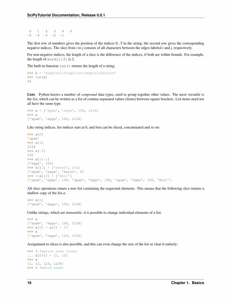
0 1 2 3 4 5-5 -4 -3 -2 -1
The first row of numbers gives the position of the indices 0...5 in the string; the second row gives the correspondingnegative indices. The slice from i to j consists of all characters between the edges labeled i and j, respectively.
For non-negative indices, the length of a slice is the difference of the indices, if both are within bounds. For example,the length of word[1:3] is 2.
The built-in function len() returns the length of a string:
>>> s = ’supercalifragilisticexpialidocious’>>> len(s)34
Lists Python knows a number of compound data types, used to group together other values. The most versatile isthe list, which can be written as a list of comma-separated values (items) between square brackets. List items need notall have the same type.
>>> a = [’spam’, ’eggs’, 100, 1234]>>> a[’spam’, ’eggs’, 100, 1234]
Like string indices, list indices start at 0, and lists can be sliced, concatenated and so on:
>>> a[0]’spam’>>> a[3]1234>>> a[-2]100>>> a[1:-1][’eggs’, 100]>>> a[:2] + [’bacon’, 2*2][’spam’, ’eggs’, ’bacon’, 4]>>> 3*a[:3] + [’Boo!’][’spam’, ’eggs’, 100, ’spam’, ’eggs’, 100, ’spam’, ’eggs’, 100, ’Boo!’]
All slice operations return a new list containing the requested elements. This means that the following slice returns ashallow copy of the list a:
>>> a[:][’spam’, ’eggs’, 100, 1234]
Unlike strings, which are immutable, it is possible to change individual elements of a list:
>>> a[’spam’, ’eggs’, 100, 1234]>>> a[2] = a[2] + 23>>> a[’spam’, ’eggs’, 123, 1234]
Assignment to slices is also possible, and this can even change the size of the list or clear it entirely:
>>> # Replace some items:... a[0:2] = [1, 12]>>> a[1, 12, 123, 1234]>>> # Remove some:
16 Chapter 1. Basics
SciPyTutorial Documentation, Release 0.0.1
... a[0:2] = []>>> a[123, 1234]>>> # Insert some:... a[1:1] = [’bletch’, ’xyzzy’]>>> a[123, ’bletch’, ’xyzzy’, 1234]>>> # Insert (a copy of) itself at the beginning>>> a[:0] = a>>> a[123, ’bletch’, ’xyzzy’, 1234, 123, ’bletch’, ’xyzzy’, 1234]>>> # Clear the list: replace all items with an empty list>>> a[:] = []>>> a[]
The built-in function len() also applies to lists:
>>> a = [’a’, ’b’, ’c’, ’d’]>>> len(a)4
It is possible to nest lists (create lists containing other lists), for example:
>>> q = [2, 3]>>> p = [1, q, 4]>>> len(p)3>>> p[1][2, 3]>>> p[1][0]2>>> p[1].append(’xtra’) # See section 5.1>>> p[1, [2, 3, ’xtra’], 4]>>> q[2, 3, ’xtra’]
Note that in the last example, p[1] and q really refer to the same object! We’ll come back to object semantics later.
First Steps Towards Programming
Of course, we can use Python for more complicated tasks than adding two and two together. For instance, we canwrite an initial sub-sequence of the Fibonacci series as follows:
>>> # Fibonacci series:... # the sum of two elements defines the next... a, b = 0, 1>>> while b < 10:... print b... a, b = b, a+b...112358
1.4. First steps in Python 17
SciPyTutorial Documentation, Release 0.0.1
This example introduces several new features.
• The first line contains a multiple assignment: the variables a and b simultaneously get the new values 0 and 1.On the last line this is used again, demonstrating that the expressions on the right-hand side are all evaluatedfirst before any of the assignments take place. The right-hand side expressions are evaluated from the left to theright.
• The while loop executes as long as the condition (here: b < 10) remains true. In Python, like in C, any non-zero integer value is true; zero is false. The condition may also be a string or list value, in fact any sequence;anything with a non-zero length is true, empty sequences are false. The test used in the example is a simplecomparison. The standard comparison operators are written the same as in C: < (less than), > (greater than), ==(equal to), <= (less than or equal to), >= (greater than or equal to) and != (not equal to).
• The body of the loop is indented: indentation is Python’s way of grouping statements. Python does not (yet!)provide an intelligent input line editing facility, so you have to type a tab or space(s) for each indented line.In practice you will prepare more complicated input for Python with a text editor; most text editors have anauto-indent facility. When a compound statement is entered interactively, it must be followed by a blank line toindicate completion (since the parser cannot guess when you have typed the last line). Note that each line withina basic block must be indented by the same amount.
• The print statement writes the value of the expression(s) it is given. It differs from just writing the expressionyou want to write (as we did earlier in the calculator examples) in the way it handles multiple expressions andstrings. Strings are printed without quotes, and a space is inserted between items, so you can format thingsnicely, like this:
>>> i = 256*256>>> print ’The value of i is’, iThe value of i is 65536
A trailing comma avoids the newline after the output:
>>> a, b = 0, 1>>> while b < 1000:... print b,... a, b = b, a+b...1 1 2 3 5 8 13 21 34 55 89 144 233 377 610 987
Note that the interpreter inserts a newline before it prints the next prompt if the last line was not completed.
Data Structures
This chapter describes some things you’ve learned about already in more detail, and adds some new things as well.
More on Lists
The list data type has some more methods. Here are all of the methods of list objects:
list.append(x)Add an item to the end of the list; equivalent to a[len(a):] = [x].
list.extend(L)Extend the list by appending all the items in the given list; equivalent to a[len(a):] = L.
list.insert(i, x)Insert an item at a given position. The first argument is the index of the element before which to in-sert, so a.insert(0, x) inserts at the front of the list, and a.insert(len(a), x) is equivalent toa.append(x).
18 Chapter 1. Basics
SciPyTutorial Documentation, Release 0.0.1
list.remove(x)Remove the first item from the list whose value is x. It is an error if there is no such item.
list.sort()Sort the items of the list, in place.
list.reverse()Reverse the elements of the list, in place.
An example that uses most of the list methods:
>>> a = [66.25, 333, 333, 1, 1234.5]>>> print a.count(333), a.count(66.25), a.count(’x’)2 1 0>>> a.insert(2, -1)>>> a.append(333)>>> a[66.25, 333, -1, 333, 1, 1234.5, 333]>>> a.index(333)1>>> a.remove(333)>>> a[66.25, -1, 333, 1, 1234.5, 333]>>> a.reverse()>>> a[333, 1234.5, 1, 333, -1, 66.25]>>> a.sort()>>> a[-1, 1, 66.25, 333, 333, 1234.5]
Functional Programming Tools There are three built-in functions that are very useful when used with lists:filter(), map(), and reduce().
filter(function, sequence) returns a sequence consisting of those items from the sequence for whichfunction(item) is true. If sequence is a string or tuple, the result will be of the same type; otherwise,it is always a list. For example, to compute some primes:
>>> def f(x): return x % 2 != 0 and x % 3 != 0...>>> filter(f, range(2, 25))[5, 7, 11, 13, 17, 19, 23]
map(function, sequence) calls function(item) for each of the sequence’s items and returns a list of thereturn values. For example, to compute some cubes:
>>> def cube(x): return x*x*x...>>> map(cube, range(1, 11))[1, 8, 27, 64, 125, 216, 343, 512, 729, 1000]
More than one sequence may be passed; the function must then have as many arguments as there are sequences andis called with the corresponding item from each sequence (or None if some sequence is shorter than another). Forexample:
>>> seq = range(8)>>> def add(x, y): return x+y...>>> map(add, seq, seq)[0, 2, 4, 6, 8, 10, 12, 14]
1.4. First steps in Python 19
SciPyTutorial Documentation, Release 0.0.1
reduce(function, sequence) returns a single value constructed by calling the binary function function onthe first two items of the sequence, then on the result and the next item, and so on. For example, to compute the sumof the numbers 1 through 10:
>>> def add(x,y): return x+y...>>> reduce(add, range(1, 11))55
If there’s only one item in the sequence, its value is returned; if the sequence is empty, an exception is raised.
A third argument can be passed to indicate the starting value. In this case the starting value is returned for an emptysequence, and the function is first applied to the starting value and the first sequence item, then to the result and thenext item, and so on. For example,
>>> def sum(seq):... def add(x,y): return x+y... return reduce(add, seq, 0)...>>> sum(range(1, 11))55>>> sum([])0
Don’t use this example’s definition of sum(): since summing numbers is such a common need, a built-in functionsum(sequence) is already provided, and works exactly like this. New in version 2.3.
List Comprehensions List comprehensions provide a concise way to create lists without resorting to use of map(),filter() and/or lambda. The resulting list definition tends often to be clearer than lists built using those con-structs. Each list comprehension consists of an expression followed by a for clause, then zero or more for or ifclauses. The result will be a list resulting from evaluating the expression in the context of the for and if clauseswhich follow it. If the expression would evaluate to a tuple, it must be parenthesized.
>>> freshfruit = [’ banana’, ’ loganberry ’, ’passion fruit ’]>>> [weapon.strip() for weapon in freshfruit][’banana’, ’loganberry’, ’passion fruit’]>>> vec = [2, 4, 6]>>> [3*x for x in vec][6, 12, 18]>>> [3*x for x in vec if x > 3][12, 18]>>> [3*x for x in vec if x < 2][]>>> [[x,x**2] for x in vec][[2, 4], [4, 16], [6, 36]]>>> [x, x**2 for x in vec] # error - parens required for tuplesFile "<stdin>", line 1, in ?[x, x**2 for x in vec]
^SyntaxError: invalid syntax>>> [(x, x**2) for x in vec][(2, 4), (4, 16), (6, 36)]>>> vec1 = [2, 4, 6]>>> vec2 = [4, 3, -9]>>> [x*y for x in vec1 for y in vec2][8, 6, -18, 16, 12, -36, 24, 18, -54]>>> [x+y for x in vec1 for y in vec2][6, 5, -7, 8, 7, -5, 10, 9, -3]
20 Chapter 1. Basics
SciPyTutorial Documentation, Release 0.0.1
>>> [vec1[i]*vec2[i] for i in range(len(vec1))][8, 12, -54]
List comprehensions are much more flexible than map() and can be applied to complex expressions and nestedfunctions:
>>> [str(round(355/113.0, i)) for i in range(1,6)][’3.1’, ’3.14’, ’3.142’, ’3.1416’, ’3.14159’]
Tuples and Sequences
We saw that lists and strings have many common properties, such as indexing and slicing operations. They are twoexamples of sequence data types (see typesseq). Since Python is an evolving language, other sequence data types maybe added. There is also another standard sequence data type: the tuple.
A tuple consists of a number of values separated by commas, for instance:
>>> t = 12345, 54321, ’hello!’>>> t[0]12345>>> t(12345, 54321, ’hello!’)>>> # Tuples may be nested:... u = t, (1, 2, 3, 4, 5)>>> u((12345, 54321, ’hello!’), (1, 2, 3, 4, 5))
As you see, on output tuples are always enclosed in parentheses, so that nested tuples are interpreted correctly; theymay be input with or without surrounding parentheses, although often parentheses are necessary anyway (if the tupleis part of a larger expression).
Tuples have many uses. For example: (x, y) coordinate pairs, employee records from a database, etc. Tuples, likestrings, are immutable: it is not possible to assign to the individual items of a tuple (you can simulate much of thesame effect with slicing and concatenation, though). It is also possible to create tuples which contain mutable objects,such as lists.
A special problem is the construction of tuples containing 0 or 1 items: the syntax has some extra quirks to accom-modate these. Empty tuples are constructed by an empty pair of parentheses; a tuple with one item is constructed byfollowing a value with a comma (it is not sufficient to enclose a single value in parentheses). Ugly, but effective. Forexample:
>>> empty = ()>>> singleton = ’hello’, # <-- note trailing comma>>> len(empty)0>>> len(singleton)1>>> singleton(’hello’,)
The statement t = 12345, 54321, ’hello!’ is an example of tuple packing: the values 12345, 54321 and’hello!’ are packed together in a tuple. The reverse operation is also possible:
>>> x, y, z = t
This is called, appropriately enough, sequence unpacking and works for any sequence on the right-hand side. Sequenceunpacking requires the list of variables on the left to have the same number of elements as the length of the sequence.Note that multiple assignment is really just a combination of tuple packing and sequence unpacking.
1.4. First steps in Python 21
SciPyTutorial Documentation, Release 0.0.1
Dictionaries
Another useful data type built into Python is the dictionary (see typesmapping). Dictionaries are sometimes found inother languages as “associative memories” or “associative arrays”. Unlike sequences, which are indexed by a rangeof numbers, dictionaries are indexed by keys, which can be any immutable type; strings and numbers can always bekeys. Tuples can be used as keys if they contain only strings, numbers, or tuples; if a tuple contains any mutable objecteither directly or indirectly, it cannot be used as a key. You can’t use lists as keys, since lists can be modified in placeusing index assignments, slice assignments, or methods like append() and extend().
It is best to think of a dictionary as an unordered set of key: value pairs, with the requirement that the keys are unique(within one dictionary). A pair of braces creates an empty dictionary: {}. Placing a comma-separated list of key:valuepairs within the braces adds initial key:value pairs to the dictionary; this is also the way dictionaries are written onoutput.
The main operations on a dictionary are storing a value with some key and extracting the value given the key. It is alsopossible to delete a key:value pair with del. If you store using a key that is already in use, the old value associatedwith that key is forgotten. It is an error to extract a value using a non-existent key.
The keys() method of a dictionary object returns a list of all the keys used in the dictionary, in arbitrary order (if youwant it sorted, just apply the sort() method to the list of keys). To check whether a single key is in the dictionary,use the in keyword.
Here is a small example using a dictionary:
>>> tel = {’jack’: 4098, ’sape’: 4139}>>> tel[’guido’] = 4127>>> tel{’sape’: 4139, ’guido’: 4127, ’jack’: 4098}>>> tel[’jack’]4098>>> del tel[’sape’]>>> tel[’irv’] = 4127>>> tel{’guido’: 4127, ’irv’: 4127, ’jack’: 4098}>>> tel.keys()[’guido’, ’irv’, ’jack’]>>> ’guido’ in telTrue
The dict() constructor builds dictionaries directly from lists of key-value pairs stored as tuples. When the pairsform a pattern, list comprehensions can compactly specify the key-value list.
>>> dict([(’sape’, 4139), (’guido’, 4127), (’jack’, 4098)]){’sape’: 4139, ’jack’: 4098, ’guido’: 4127}>>> dict([(x, x**2) for x in (2, 4, 6)]) # use a list comprehension{2: 4, 4: 16, 6: 36}
Later in the tutorial, we will learn about Generator Expressions which are even better suited for the task of supplyingkey-values pairs to the dict() constructor.
When the keys are simple strings, it is sometimes easier to specify pairs using keyword arguments:
>>> dict(sape=4139, guido=4127, jack=4098){’sape’: 4139, ’jack’: 4098, ’guido’: 4127}
22 Chapter 1. Basics
SciPyTutorial Documentation, Release 0.0.1
Looping Techniques
When looping through dictionaries, the key and corresponding value can be retrieved at the same time using theiteritems() method.
>>> knights = {’gallahad’: ’the pure’, ’robin’: ’the brave’}>>> for k, v in knights.iteritems():... print k, v...gallahad the purerobin the brave
When looping through a sequence, the position index and corresponding value can be retrieved at the same time usingthe enumerate() function.
>>> for i, v in enumerate([’tic’, ’tac’, ’toe’]):... print i, v...0 tic1 tac2 toe
To loop over two or more sequences at the same time, the entries can be paired with the zip() function.
>>> questions = [’name’, ’quest’, ’favorite color’]>>> answers = [’lancelot’, ’the holy grail’, ’blue’]>>> for q, a in zip(questions, answers):... print ’What is your {0}? It is {1}.’.format(q, a)...What is your name? It is lancelot.What is your quest? It is the holy grail.What is your favorite color? It is blue.
To loop over a sequence in reverse, first specify the sequence in a forward direction and then call the reversed()function.
>>> for i in reversed(xrange(1,10,2)):... print i...97531
To loop over a sequence in sorted order, use the sorted() function which returns a new sorted list while leaving thesource unaltered.
>>> basket = [’apple’, ’orange’, ’apple’, ’pear’, ’orange’, ’banana’]>>> for f in sorted(set(basket)):... print f...applebananaorangepear
1.4. First steps in Python 23
SciPyTutorial Documentation, Release 0.0.1
More on Conditions
The conditions used in while and if statements can contain any operators, not just comparisons.
The comparison operators in and not in check whether a value occurs (does not occur) in a sequence. The operatorsis and is not compare whether two objects are really the same object; this only matters for mutable objects likelists. All comparison operators have the same priority, which is lower than that of all numerical operators.
Comparisons can be chained. For example, a < b == c tests whether a is less than b and moreover b equals c.
Comparisons may be combined using the Boolean operators and and or, and the outcome of a comparison (or of anyother Boolean expression) may be negated with not. These have lower priorities than comparison operators; betweenthem, not has the highest priority and or the lowest, so that A and not B or C is equivalent to (A and (notB)) or C. As always, parentheses can be used to express the desired composition.
The Boolean operators and and or are so-called short-circuit operators: their arguments are evaluated from left toright, and evaluation stops as soon as the outcome is determined. For example, if A and C are true but B is false, Aand B and C does not evaluate the expression C. When used as a general value and not as a Boolean, the returnvalue of a short-circuit operator is the last evaluated argument.
It is possible to assign the result of a comparison or other Boolean expression to a variable. For example,
>>> string1, string2, string3 = ’’, ’Trondheim’, ’Hammer Dance’>>> non_null = string1 or string2 or string3>>> non_null’Trondheim’
Note that in Python, unlike C, assignment cannot occur inside expressions. C programmers may grumble about this,but it avoids a common class of problems encountered in C programs: typing = in an expression when ==was intended.
More Control Flow Tools
Besides the while statement just introduced, Python knows the usual control flow statements known from otherlanguages, with some twists.
if Statements
Perhaps the most well-known statement type is the if statement. For example:
>>> x = int(raw_input("Please enter an integer: "))Please enter an integer: 42>>> if x < 0:... x = 0... print ’Negative changed to zero’... elif x == 0:... print ’Zero’... elif x == 1:... print ’Single’... else:... print ’More’...More
There can be zero or more elif parts, and the else part is optional. The keyword ‘elif‘ is short for ‘else if’, andis useful to avoid excessive indentation. An if ... elif ... elif ... sequence is a substitute for the switch or casestatements found in other languages.
24 Chapter 1. Basics
SciPyTutorial Documentation, Release 0.0.1
for Statements
The for statement in Python differs a bit from what you may be used to in C or Pascal. Rather than always iteratingover an arithmetic progression of numbers (like in Pascal), or giving the user the ability to define both the iterationstep and halting condition (as C), Python’s for statement iterates over the items of any sequence (a list or a string), inthe order that they appear in the sequence. For example (no pun intended):
>>> # Measure some strings:... a = [’cat’, ’window’, ’defenestrate’]>>> for x in a:... print x, len(x)...cat 3window 6defenestrate 12
It is not safe to modify the sequence being iterated over in the loop (this can only happen for mutable sequence types,such as lists). If you need to modify the list you are iterating over (for example, to duplicate selected items) you mustiterate over a copy. The slice notation makes this particularly convenient:
>>> for x in a[:]: # make a slice copy of the entire list... if len(x) > 6: a.insert(0, x)...>>> a[’defenestrate’, ’cat’, ’window’, ’defenestrate’]
The range() Function
If you do need to iterate over a sequence of numbers, the built-in function range() comes in handy. It generates listscontaining arithmetic progressions:
>>> range(10)[0, 1, 2, 3, 4, 5, 6, 7, 8, 9]
The given end point is never part of the generated list; range(10) generates a list of 10 values, the legal indicesfor items of a sequence of length 10. It is possible to let the range start at another number, or to specify a differentincrement (even negative; sometimes this is called the ‘step’):
>>> range(5, 10)[5, 6, 7, 8, 9]>>> range(0, 10, 3)[0, 3, 6, 9]>>> range(-10, -100, -30)[-10, -40, -70]
To iterate over the indices of a sequence, you can combine range() and len() as follows:
>>> a = [’Mary’, ’had’, ’a’, ’little’, ’lamb’]>>> for i in range(len(a)):... print i, a[i]...0 Mary1 had2 a3 little4 lamb
In most such cases, however, it is convenient to use the enumerate() function, see Looping Techniques.
1.4. First steps in Python 25
SciPyTutorial Documentation, Release 0.0.1
break and continue Statements, and else Clauses on Loops
The break statement, like in C, breaks out of the smallest enclosing for or while loop.
The continue statement, also borrowed from C, continues with the next iteration of the loop.
Loop statements may have an else clause; it is executed when the loop terminates through exhaustion of the list (withfor) or when the condition becomes false (with while), but not when the loop is terminated by a break statement.This is exemplified by the following loop, which searches for prime numbers:
>>> for n in range(2, 10):... for x in range(2, n):... if n % x == 0:... print n, ’equals’, x, ’*’, n/x... break... else:... # loop fell through without finding a factor... print n, ’is a prime number’...2 is a prime number3 is a prime number4 equals 2 * 25 is a prime number6 equals 2 * 37 is a prime number8 equals 2 * 49 equals 3 * 3
pass Statements
The pass statement does nothing. It can be used when a statement is required syntactically but the program requiresno action. For example:
>>> while True:... pass # Busy-wait for keyboard interrupt (Ctrl+C)...
This is commonly used for creating minimal classes:
>>> class MyEmptyClass:... pass...
Another place pass can be used is as a place-holder for a function or conditional body when you are working on newcode, allowing you to keep thinking at a more abstract level. The pass is silently ignored:
>>> def initlog(*args):... pass # Remember to implement this!...
Defining Functions
We can create a function that writes the Fibonacci series to an arbitrary boundary:
>>> def fib(n): # write Fibonacci series up to n... """Print a Fibonacci series up to n."""
26 Chapter 1. Basics
SciPyTutorial Documentation, Release 0.0.1
... a, b = 0, 1
... while a < n:
... print a,
... a, b = b, a+b
...>>> # Now call the function we just defined:... fib(2000)0 1 1 2 3 5 8 13 21 34 55 89 144 233 377 610 987 1597
The keyword def introduces a function definition. It must be followed by the function name and the parenthesized listof formal parameters. The statements that form the body of the function start at the next line, and must be indented.
The first statement of the function body can optionally be a string literal; this string literal is the function’s documenta-tion string, or docstring. (More about docstrings can be found in the section tut-docstrings.) There are tools which usedocstrings to automatically produce online or printed documentation, or to let the user interactively browse throughcode; it’s good practice to include docstrings in code that you write, so make a habit of it.
The execution of a function introduces a new symbol table used for the local variables of the function. More precisely,all variable assignments in a function store the value in the local symbol table; whereas variable references first lookin the local symbol table, then in the local symbol tables of enclosing functions, then in the global symbol table, andfinally in the table of built-in names. Thus, global variables cannot be directly assigned a value within a function(unless named in a global statement), although they may be referenced.
The actual parameters (arguments) to a function call are introduced in the local symbol table of the called functionwhen it is called; thus, arguments are passed using call by value (where the value is always an object reference, notthe value of the object). 1 When a function calls another function, a new local symbol table is created for that call.
A function definition introduces the function name in the current symbol table. The value of the function name has atype that is recognized by the interpreter as a user-defined function. This value can be assigned to another name whichcan then also be used as a function. This serves as a general renaming mechanism:
>>> fib<function fib at 10042ed0>>>> f = fib>>> f(100)0 1 1 2 3 5 8 13 21 34 55 89
Coming from other languages, you might object that fib is not a function but a procedure since it doesn’t return avalue. In fact, even functions without a return statement do return a value, albeit a rather boring one. This value iscalled None (it’s a built-in name). Writing the value None is normally suppressed by the interpreter if it would be theonly value written. You can see it if you really want to using print:
>>> fib(0)>>> print fib(0)None
It is simple to write a function that returns a list of the numbers of the Fibonacci series, instead of printing it:
>>> def fib2(n): # return Fibonacci series up to n... """Return a list containing the Fibonacci series up to n."""... result = []... a, b = 0, 1... while a < n:... result.append(a) # see below... a, b = b, a+b... return result...
1 Actually, call by object reference would be a better description, since if a mutable object is passed, the caller will see any changes the calleemakes to it (items inserted into a list).
1.4. First steps in Python 27
SciPyTutorial Documentation, Release 0.0.1
>>> f100 = fib2(100) # call it>>> f100 # write the result[0, 1, 1, 2, 3, 5, 8, 13, 21, 34, 55, 89]
This example, as usual, demonstrates some new Python features:
• The return statement returns with a value from a function. return without an expression argument returnsNone. Falling off the end of a function also returns None.
• The statement result.append(a) calls a method of the list object result. A method is a function that‘belongs’ to an object and is named obj.methodname, where obj is some object (this may be an expression),and methodname is the name of a method that is defined by the object’s type. Different types define differentmethods. Methods of different types may have the same name without causing ambiguity. (It is possible todefine your own object types and methods, using classes, see Classes) The method append() shown in theexample is defined for list objects; it adds a new element at the end of the list. In this example it is equivalent toresult = result + [a], but more efficient.
More on Defining Functions
It is also possible to define functions with a variable number of arguments. There are three forms, which can becombined.
Default Argument Values The most useful form is to specify a default value for one or more arguments. Thiscreates a function that can be called with fewer arguments than it is defined to allow. For example:
def ask_ok(prompt, retries=4, complaint=’Yes or no, please!’):while True:
ok = raw_input(prompt)if ok in (’y’, ’ye’, ’yes’):
return Trueif ok in (’n’, ’no’, ’nop’, ’nope’):
return Falseretries = retries - 1if retries < 0:
raise IOError(’refusenik user’)print complaint
This function can be called in several ways:
• giving only the mandatory argument: ask_ok(’Do you really want to quit?’)
• giving one of the optional arguments: ask_ok(’OK to overwrite the file?’, 2)
• or even giving all arguments: ask_ok(’OK to overwrite the file?’, 2, ’Come on, onlyyes or no!’)
This example also introduces the in keyword. This tests whether or not a sequence contains a certain value.
The default values are evaluated at the point of function definition in the defining scope, so that
i = 5
def f(arg=i):print arg
i = 6f()
28 Chapter 1. Basics
SciPyTutorial Documentation, Release 0.0.1
will print 5.
Important warning: The default value is evaluated only once. This makes a difference when the default is a mutableobject such as a list, dictionary, or instances of most classes. For example, the following function accumulates thearguments passed to it on subsequent calls:
def f(a, L=[]):L.append(a)return L
print f(1)print f(2)print f(3)
This will print
[1][1, 2][1, 2, 3]
If you don’t want the default to be shared between subsequent calls, you can write the function like this instead:
def f(a, L=None):if L is None:
L = []L.append(a)return L
Keyword Arguments Functions can also be called using keyword arguments of the form keyword = value.For instance, the following function:
def parrot(voltage, state=’a stiff’, action=’voom’, type=’Norwegian Blue’):print "-- This parrot wouldn’t", action,print "if you put", voltage, "volts through it."print "-- Lovely plumage, the", typeprint "-- It’s", state, "!"
could be called in any of the following ways:
parrot(1000)parrot(action = ’VOOOOOM’, voltage = 1000000)parrot(’a thousand’, state = ’pushing up the daisies’)parrot(’a million’, ’bereft of life’, ’jump’)
but the following calls would all be invalid:
parrot() # required argument missingparrot(voltage=5.0, ’dead’) # non-keyword argument following keywordparrot(110, voltage=220) # duplicate value for argumentparrot(actor=’John Cleese’) # unknown keyword
In general, an argument list must have any positional arguments followed by any keyword arguments, where thekeywords must be chosen from the formal parameter names. It’s not important whether a formal parameter has adefault value or not. No argument may receive a value more than once — formal parameter names corresponding topositional arguments cannot be used as keywords in the same calls. Here’s an example that fails due to this restriction:
>>> def function(a):... pass...
1.4. First steps in Python 29
SciPyTutorial Documentation, Release 0.0.1
>>> function(0, a=0)Traceback (most recent call last):
File "<stdin>", line 1, in ?TypeError: function() got multiple values for keyword argument ’a’
When a final formal parameter of the form **name is present, it receives a dictionary (see typesmapping) containingall keyword arguments except for those corresponding to a formal parameter. This may be combined with a formalparameter of the form *name (described in the next subsection) which receives a tuple containing the positionalarguments beyond the formal parameter list. (*name must occur before **name.) For example, if we define afunction like this:
def cheeseshop(kind, *arguments, **keywords):print "-- Do you have any", kind, "?"print "-- I’m sorry, we’re all out of", kindfor arg in arguments: print argprint "-" * 40keys = keywords.keys()keys.sort()for kw in keys: print kw, ":", keywords[kw]
It could be called like this:
cheeseshop("Limburger", "It’s very runny, sir.","It’s really very, VERY runny, sir.",shopkeeper=’Michael Palin’,client="John Cleese",sketch="Cheese Shop Sketch")
and of course it would print:
-- Do you have any Limburger ?-- I’m sorry, we’re all out of LimburgerIt’s very runny, sir.It’s really very, VERY runny, sir.----------------------------------------client : John Cleeseshopkeeper : Michael Palinsketch : Cheese Shop Sketch
Note that the sort() method of the list of keyword argument names is called before printing the contents of thekeywords dictionary; if this is not done, the order in which the arguments are printed is undefined.
Lambda Forms By popular demand, a few features commonly found in functional programming languages like Lisphave been added to Python. With the lambda keyword, small anonymous functions can be created. Here’s a functionthat returns the sum of its two arguments: lambda a, b: a+b. Lambda forms can be used wherever functionobjects are required. They are syntactically restricted to a single expression. Semantically, they are just syntacticsugar for a normal function definition. Like nested function definitions, lambda forms can reference variables fromthe containing scope:
>>> def make_incrementor(n):... return lambda x: x + n...>>> f = make_incrementor(42)>>> f(0)42>>> f(1)43
30 Chapter 1. Basics
SciPyTutorial Documentation, Release 0.0.1
Classes
Python’s class mechanism adds classes to the language with a minimum of new syntax and semantics. It is a mixtureof the class mechanisms found in C++ and Modula-3. As is true for modules, classes in Python do not put an absolutebarrier between definition and user, but rather rely on the politeness of the user not to “break into the definition.”The most important features of classes are retained with full power, however: the class inheritance mechanism allowsmultiple base classes, a derived class can override any methods of its base class or classes, and a method can call themethod of a base class with the same name. Objects can contain an arbitrary amount of data.
In C++ terminology, all class members (including the data members) are public, and all member functions are virtual.As in Modula-3, there are no shorthands for referencing the object’s members from its methods: the method functionis declared with an explicit first argument representing the object, which is provided implicitly by the call. As inSmalltalk, classes themselves are objects. This provides semantics for importing and renaming. Unlike C++ andModula-3, built-in types can be used as base classes for extension by the user. Also, like in C++, most built-inoperators with special syntax (arithmetic operators, subscripting etc.) can be redefined for class instances.
(Lacking universally accepted terminology to talk about classes, I will make occasional use of Smalltalk and C++terms. I would use Modula-3 terms, since its object-oriented semantics are closer to those of Python than C++, but Iexpect that few readers have heard of it.)
A First Look at Classes
Classes introduce a little bit of new syntax, three new object types, and some new semantics.
Class Definition Syntax The simplest form of class definition looks like this:
class ClassName:<statement-1>...<statement-N>
Class definitions, like function definitions (def statements) must be executed before they have any effect. (You couldconceivably place a class definition in a branch of an if statement, or inside a function.)
In practice, the statements inside a class definition will usually be function definitions, but other statements are allowed,and sometimes useful — we’ll come back to this later. The function definitions inside a class normally have a peculiarform of argument list, dictated by the calling conventions for methods — again, this is explained later.
When a class definition is entered, a new namespace is created, and used as the local scope — thus, all assignments tolocal variables go into this new namespace. In particular, function definitions bind the name of the new function here.
When a class definition is left normally (via the end), a class object is created. This is basically a wrapper around thecontents of the namespace created by the class definition; we’ll learn more about class objects in the next section. Theoriginal local scope (the one in effect just before the class definition was entered) is reinstated, and the class object isbound here to the class name given in the class definition header (ClassName in the example).
Class Objects Class objects support two kinds of operations: attribute references and instantiation.
Attribute references use the standard syntax used for all attribute references in Python: obj.name. Valid attributenames are all the names that were in the class’s namespace when the class object was created. So, if the class definitionlooked like this:
1.4. First steps in Python 31
SciPyTutorial Documentation, Release 0.0.1
class MyClass:"""A simple example class"""i = 12345def f(self):
return ’hello world’
then MyClass.i and MyClass.f are valid attribute references, returning an integer and a function object, respec-tively. Class attributes can also be assigned to, so you can change the value of MyClass.i by assignment. __doc__is also a valid attribute, returning the docstring belonging to the class: "A simple example class".
Class instantiation uses function notation. Just pretend that the class object is a parameterless function that returns anew instance of the class. For example (assuming the above class):
x = MyClass()
creates a new instance of the class and assigns this object to the local variable x.
The instantiation operation (“calling” a class object) creates an empty object. Many classes like to create objects withinstances customized to a specific initial state. Therefore a class may define a special method named __init__(),like this:
def __init__(self):self.data = []
When a class defines an __init__() method, class instantiation automatically invokes __init__() for thenewly-created class instance. So in this example, a new, initialized instance can be obtained by:
x = MyClass()
Of course, the __init__() method may have arguments for greater flexibility. In that case, arguments given to theclass instantiation operator are passed on to __init__(). For example,
>>> class Complex:... def __init__(self, realpart, imagpart):... self.r = realpart... self.i = imagpart...>>> x = Complex(3.0, -4.5)>>> x.r, x.i(3.0, -4.5)
Instance Objects Now what can we do with instance objects? The only operations understood by instance objectsare attribute references. There are two kinds of valid attribute names, data attributes and methods.
data attributes correspond to “instance variables” in Smalltalk, and to “data members” in C++. Data attributes neednot be declared; like local variables, they spring into existence when they are first assigned to. For example, if x is theinstance of MyClass created above, the following piece of code will print the value 16, without leaving a trace:
x.counter = 1while x.counter < 10:
x.counter = x.counter * 2print x.counterdel x.counter
The other kind of instance attribute reference is a method. A method is a function that “belongs to” an object. (InPython, the term method is not unique to class instances: other object types can have methods as well. For example,list objects have methods called append, insert, remove, sort, and so on. However, in the following discussion, we’lluse the term method exclusively to mean methods of class instance objects, unless explicitly stated otherwise.) Validmethod names of an instance object depend on its class. By definition, all attributes of a class that are function objects
32 Chapter 1. Basics
SciPyTutorial Documentation, Release 0.0.1
define corresponding methods of its instances. So in our example, x.f is a valid method reference, since MyClass.fis a function, but x.i is not, since MyClass.i is not. But x.f is not the same thing as MyClass.f— it is a methodobject, not a function object.
Method Objects Usually, a method is called right after it is bound:
x.f()
In the MyClass example, this will return the string ’hello world’. However, it is not necessary to call a methodright away: x.f is a method object, and can be stored away and called at a later time. For example:
xf = x.fwhile True:
print xf()
will continue to print hello world until the end of time.
What exactly happens when a method is called? You may have noticed that x.f() was called without an argumentabove, even though the function definition for f() specified an argument. What happened to the argument? SurelyPython raises an exception when a function that requires an argument is called without any — even if the argumentisn’t actually used...
Actually, you may have guessed the answer: the special thing about methods is that the object is passed as the firstargument of the function. In our example, the call x.f() is exactly equivalent to MyClass.f(x). In general,calling a method with a list of n arguments is equivalent to calling the corresponding function with an argument listthat is created by inserting the method’s object before the first argument.
If you still don’t understand how methods work, a look at the implementation can perhaps clarify matters. When aninstance attribute is referenced that isn’t a data attribute, its class is searched. If the name denotes a valid class attributethat is a function object, a method object is created by packing (pointers to) the instance object and the function objectjust found together in an abstract object: this is the method object. When the method object is called with an argumentlist, a new argument list is constructed from the instance object and the argument list, and the function object is calledwith this new argument list.
Random Remarks
Data attributes override method attributes with the same name; to avoid accidental name conflicts, which may causehard-to-find bugs in large programs, it is wise to use some kind of convention that minimizes the chance of conflicts.Possible conventions include capitalizing method names, prefixing data attribute names with a small unique string(perhaps just an underscore), or using verbs for methods and nouns for data attributes.
Data attributes may be referenced by methods as well as by ordinary users (“clients”) of an object. In other words,classes are not usable to implement pure abstract data types. In fact, nothing in Python makes it possible to enforcedata hiding — it is all based upon convention. (On the other hand, the Python implementation, written in C, cancompletely hide implementation details and control access to an object if necessary; this can be used by extensions toPython written in C.)
Clients should use data attributes with care — clients may mess up invariants maintained by the methods by stampingon their data attributes. Note that clients may add data attributes of their own to an instance object without affectingthe validity of the methods, as long as name conflicts are avoided — again, a naming convention can save a lot ofheadaches here.
There is no shorthand for referencing data attributes (or other methods!) from within methods. I find that this actuallyincreases the readability of methods: there is no chance of confusing local variables and instance variables whenglancing through a method.
1.4. First steps in Python 33
SciPyTutorial Documentation, Release 0.0.1
Often, the first argument of a method is called self. This is nothing more than a convention: the name self hasabsolutely no special meaning to Python. Note, however, that by not following the convention your code may be lessreadable to other Python programmers, and it is also conceivable that a class browser program might be written thatrelies upon such a convention.
Any function object that is a class attribute defines a method for instances of that class. It is not necessary that thefunction definition is textually enclosed in the class definition: assigning a function object to a local variable in theclass is also ok. For example:
# Function defined outside the classdef f1(self, x, y):
return min(x, x+y)
class C:f = f1def g(self):
return ’hello world’h = g
Now f, g and h are all attributes of class C that refer to function objects, and consequently they are all methods ofinstances of C — h being exactly equivalent to g. Note that this practice usually only serves to confuse the reader of aprogram.
Methods may call other methods by using method attributes of the self argument:
class Bag:def __init__(self):
self.data = []def add(self, x):
self.data.append(x)def addtwice(self, x):
self.add(x)self.add(x)
Methods may reference global names in the same way as ordinary functions. The global scope associated with amethod is the module containing the class definition. (The class itself is never used as a global scope.) While onerarely encounters a good reason for using global data in a method, there are many legitimate uses of the global scope:for one thing, functions and modules imported into the global scope can be used by methods, as well as functions andclasses defined in it. Usually, the class containing the method is itself defined in this global scope, and in the nextsection we’ll find some good reasons why a method would want to reference its own class.
Each value is an object, and therefore has a class (also called its type). It is stored as object.__class__.
Iterators
By now you have probably noticed that most container objects can be looped over using a for statement:
for element in [1, 2, 3]:print element
for element in (1, 2, 3):print element
for key in {’one’:1, ’two’:2}:print key
for char in "123":print char
for line in open("myfile.txt"):print line
34 Chapter 1. Basics
SciPyTutorial Documentation, Release 0.0.1
This style of access is clear, concise, and convenient. The use of iterators pervades and unifies Python. Behind thescenes, the for statement calls iter() on the container object. The function returns an iterator object that definesthe method next() which accesses elements in the container one at a time. When there are no more elements,next() raises a StopIteration exception which tells the for loop to terminate. This example shows how it allworks:
>>> s = ’abc’>>> it = iter(s)>>> it<iterator object at 0x00A1DB50>>>> it.next()’a’>>> it.next()’b’>>> it.next()’c’>>> it.next()
Traceback (most recent call last):File "<stdin>", line 1, in ?it.next()
StopIteration
Having seen the mechanics behind the iterator protocol, it is easy to add iterator behavior to your classes. Definean __iter__() method which returns an object with a next() method. If the class defines next(), then__iter__() can just return self:
class Reverse:"Iterator for looping over a sequence backwards"def __init__(self, data):
self.data = dataself.index = len(data)
def __iter__(self):return self
def next(self):if self.index == 0:
raise StopIterationself.index = self.index - 1return self.data[self.index]
>>> rev = Reverse(’spam’)>>> iter(rev)<__main__.Reverse object at 0x00A1DB50>>>> for char in rev:... print char...maps
Python Packages
Required, optional or otherwise noteworthy python packages are presented in the following short table. We do notpretend that this table is in any way exhaustive. For a much more comprehensive list take a look at the Python packageindex at: http://pypi.python.org/pypi.
• numpy
1.4. First steps in Python 35
SciPyTutorial Documentation, Release 0.0.1
NumPy is the fundamental package needed for scientific computing with Python. It contains among other thingsa powerful N-dimensional array object
– URL: http://www.numpy.org/
• scipy
The SciPy library is built to work with NumPy arrays, and provides many user-friendly and efficient numericalroutines such as routines for optimization, linear algebra, integration, interpolation, special functions, FFT,signal and image processing, ODE solvers and other tasks common in science and engineering.
– URL: http://www.scipy.org/
• matplotlib
Matplotlib is a python 2D plotting library for the Python programming language which produces publicationquality figures in a variety of formats. You can generate plots, histograms, power spectra, bar charts, errorcharts,scatterplots, etc, with just a few lines of code.
– URL: http://matplotlib.sourceforge.net/
• sympy
SymPy is a Python library for (limited) symbolic computations inside python programms.
– URL: http://sympy.org/
• PIL
Python Imaging Library is a library for the Python programming language that provides support for opening,manipulating, and saving many different image file formats.
– URL: http://www.pythonware.com/products/pil/
• mpmath
Mpmath is a Python library for multiprecision floating-point arithmetic. It provides an extensive set of transcen-dental functions, unlimited exponent sizes, complex numbers, interval arithmetic, numerical integration anddifferentiation, root-finding, linear algebra, and much more
– URL: http://code.google.com/p/mpmath/
• MeshPy
MeshPy offers quality triangular and tetrahedral mesh generation for Python. Meshes of this type are chieflyused in finite-element simulation codes, but also have many other applications ranging from computer graphicsto robotics.
– URL: http://mathema.tician.de/software/meshpy
• PyX
PyX is a Python package for the creation of PostScript and PDF files. It combines an abstraction of the PostScriptdrawing model with a TeX/LaTeX interface. This package can be used for two dimensional (geometric) draw-ings.
– URL: http://pyx.sourceforge.net/
• h5py
The HDF5 library is a versatile, mature library designed for the storage of numerical data. The h5py packageprovides a simple, Pythonic interface to HDF5. A straightforward high-level interface allows the manipulationof HDF5 files, groups and datasets using established Python and NumPy metaphors.
– URL: http://h5py.alfven.org/
36 Chapter 1. Basics
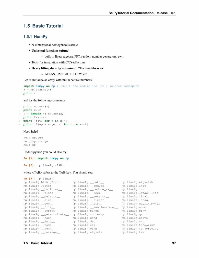
SciPyTutorial Documentation, Release 0.0.1
1.5 Basic Tutorial
1.5.1 NumPy
• N-dimensional homogeneous arrays
• Universal functions (ufunc)
– built-in linear algebra, FFT, random number generators, etc...
• Tools for integration with C/C++/Fortran
• Heavy lifting done by optimized C/Fortran libraries
– ATLAS, UMFPACK, FFTW, etc...
Let us initialize an array with first n natural numbers:
import numpy as np # import the module and use a shorter namespacex = np.arange(4)print x
and try the following commands:
1 print np.sum(x)2 print x**23 f = lambda x: np.sum(x)4 print f(x**2)5 print [f(t) for t in x**2]6 print [f(np.arange(t)) for t in x**2]
Need help?
help np.sumhelp np.arangehelp np
Under ipython you could also try:
In [1]: import numpy as np
In [2]: np.linalg.<TAB>
where <TAB> refers to the TAB-key. You should see:
In [2]: np.linalg.np.linalg.LinAlgError np.linalg.__path__ np.linalg.eigvalshnp.linalg.Tester np.linalg.__reduce__ np.linalg.infonp.linalg.__builtins__ np.linalg.__reduce_ex__ np.linalg.invnp.linalg.__class__ np.linalg.__repr__ np.linalg.lapack_litenp.linalg.__delattr__ np.linalg.__setattr__ np.linalg.linalgnp.linalg.__dict__ np.linalg.__sizeof__ np.linalg.lstsqnp.linalg.__doc__ np.linalg.__str__ np.linalg.matrix_powernp.linalg.__file__ np.linalg.__subclasshook__ np.linalg.normnp.linalg.__format__ np.linalg.bench np.linalg.pinvnp.linalg.__getattribute__ np.linalg.cholesky np.linalg.qrnp.linalg.__hash__ np.linalg.cond np.linalg.solvenp.linalg.__init__ np.linalg.det np.linalg.svdnp.linalg.__name__ np.linalg.eig np.linalg.tensorinvnp.linalg.__new__ np.linalg.eigh np.linalg.tensorsolvenp.linalg.__package__ np.linalg.eigvals np.linalg.test
1.5. Basic Tutorial 37
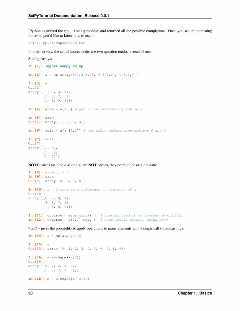
SciPyTutorial Documentation, Release 0.0.1
IPython examined the np.linalg module, and returned all the possible completions. Once you see an interestingfunction, you’d like to know how to use it:
In[3]: np.transpose?<ENTER>
In order to view the actual source code, use two question marks instead of one.
Slicing Arrays:
In [1]: import numpy as np
In [2]: a = np.array([[1,2,3,4],[9,8,7,6],[1,6,5,4]])
In [3]: aOut[3]:array([[1, 2, 3, 4],
[9, 8, 7, 6],[1, 6, 5, 4]])
In [4]: arow = a[0,:] # get slice referencing row zero
In [5]: arowOut[5]: array([1, 2, 3, 4])
In [6]: cols = a[:,[0,2]] # get slice referencing columns 0 and 2
In [7]: colsOut[7]:array([[1, 3],
[9, 7],[1, 5]])
NOTE: slices (as arow & cols) are NOT copies, they point to the original data:
In [8]: arow[:] = 0In [9]: arowOut[9]: array([0, 0, 0, 0])
In [10]: a # arow is a reference to elements of aOut[10]:array([[0, 0, 0, 0],
[9, 8, 7, 6],[1, 6, 5, 4]])
In [11]: copyrow = arow.copy() # copying need to be invoked explicitlyIn [11]: copyrow = a[0,:].copy() # same result without using arow
NumPy gives the possibility to apply operations to many elements with a single call (broadcasting):
In [14]: a = np.arange(10)
In [15]: aOut[15]: array([0, 1, 2, 3, 4, 5, 6, 7, 8, 9])
In [16]: a.reshape((2,5))Out[16]:array([[0, 1, 2, 3, 4],
[5, 6, 7, 8, 9]])
In [18]: b = a.reshape((2,5))
38 Chapter 1. Basics
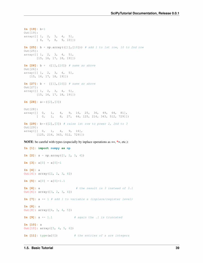
SciPyTutorial Documentation, Release 0.0.1
In [19]: b+1Out[19]:array([[ 1, 2, 3, 4, 5],
[ 6, 7, 8, 9, 10]])
In [25]: b + np.array(([1],[10])) # add 1 to 1st row, 10 to 2nd rowOut[25]:array([[ 1, 2, 3, 4, 5],
[15, 16, 17, 18, 19]])
In [26]: b + ([1],[10]) # same as aboveOut[26]:array([[ 1, 2, 3, 4, 5],
[15, 16, 17, 18, 19]])
In [27]: b + [[1],[10]] # same as aboveOut[27]:array([[ 1, 2, 3, 4, 5],
[15, 16, 17, 18, 19]])
In [28]: a**([2],[3])
Out[28]:array([[ 0, 1, 4, 9, 16, 25, 36, 49, 64, 81],
[ 0, 1, 8, 27, 64, 125, 216, 343, 512, 729]])
In [29]: b**([2],[3]) # raise 1st row to power 2, 2nd to 3Out[29]:array([[ 0, 1, 4, 9, 16],
[125, 216, 343, 512, 729]])
NOTE: be careful with types (especially by inplace operations as +=, *=, etc.):
In [1]: import numpy as np
In [2]: a = np.array([1, 2, 3, 4])
In [3]: a[0] = a[0]+1
In [4]: aOut[4]: array([2, 2, 3, 4])
In [5]: a[0] = a[0]+1.1
In [6]: a # the result is 3 instead of 3.1Out[6]: array([3, 2, 3, 4])
In [7]: a += 1 # add 1 to variable a (inplace/register level)
In [8]: aOut[8]: array([4, 3, 4, 5])
In [9]: a += 1.1 # again the .1 is truncated
In [10]: aOut[10]: array([5, 4, 5, 6])
In [11]: type(a[0]) # the entries of a are integers
1.5. Basic Tutorial 39
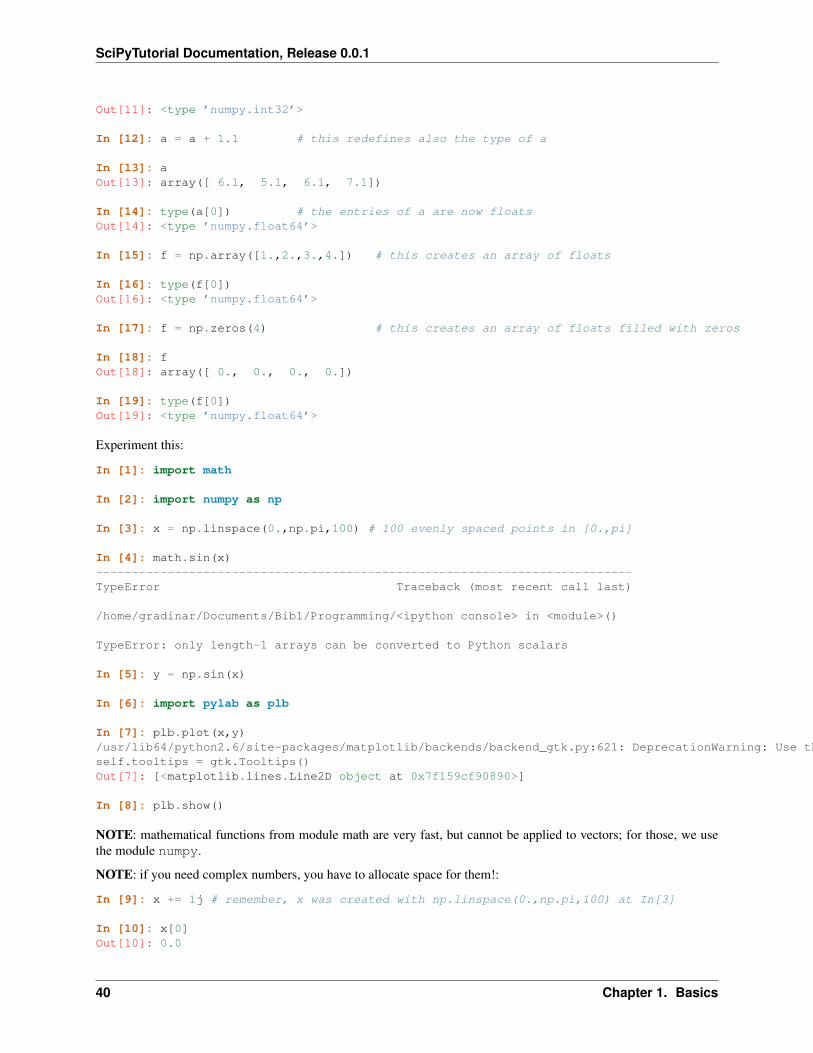
SciPyTutorial Documentation, Release 0.0.1
Out[11]: <type ’numpy.int32’>
In [12]: a = a + 1.1 # this redefines also the type of a
In [13]: aOut[13]: array([ 6.1, 5.1, 6.1, 7.1])
In [14]: type(a[0]) # the entries of a are now floatsOut[14]: <type ’numpy.float64’>
In [15]: f = np.array([1.,2.,3.,4.]) # this creates an array of floats
In [16]: type(f[0])Out[16]: <type ’numpy.float64’>
In [17]: f = np.zeros(4) # this creates an array of floats filled with zeros
In [18]: fOut[18]: array([ 0., 0., 0., 0.])
In [19]: type(f[0])Out[19]: <type ’numpy.float64’>
Experiment this:
In [1]: import math
In [2]: import numpy as np
In [3]: x = np.linspace(0.,np.pi,100) # 100 evenly spaced points in [0.,pi]
In [4]: math.sin(x)---------------------------------------------------------------------------TypeError Traceback (most recent call last)
/home/gradinar/Documents/Bibl/Programming/<ipython console> in <module>()
TypeError: only length-1 arrays can be converted to Python scalars
In [5]: y = np.sin(x)
In [6]: import pylab as plb
In [7]: plb.plot(x,y)/usr/lib64/python2.6/site-packages/matplotlib/backends/backend_gtk.py:621: DeprecationWarning: Use the new widget gtk.Tooltipself.tooltips = gtk.Tooltips()Out[7]: [<matplotlib.lines.Line2D object at 0x7f159cf90890>]
In [8]: plb.show()
NOTE: mathematical functions from module math are very fast, but cannot be applied to vectors; for those, we usethe module numpy.
NOTE: if you need complex numbers, you have to allocate space for them!:
In [9]: x += 1j # remember, x was created with np.linspace(0.,np.pi,100) at In[3]
In [10]: x[0]Out[10]: 0.0
40 Chapter 1. Basics
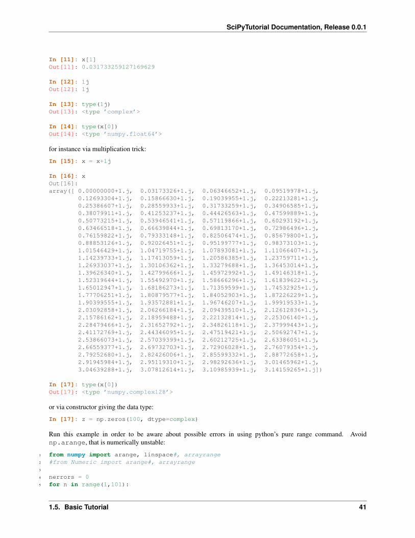
SciPyTutorial Documentation, Release 0.0.1
In [11]: x[1]Out[11]: 0.031733259127169629
In [12]: 1jOut[12]: 1j
In [13]: type(1j)Out[13]: <type ’complex’>
In [14]: type(x[0])Out[14]: <type ’numpy.float64’>
for instance via multiplication trick:
In [15]: x = x+1j
In [16]: xOut[16]:array([ 0.00000000+1.j, 0.03173326+1.j, 0.06346652+1.j, 0.09519978+1.j,
0.12693304+1.j, 0.15866630+1.j, 0.19039955+1.j, 0.22213281+1.j,0.25386607+1.j, 0.28559933+1.j, 0.31733259+1.j, 0.34906585+1.j,0.38079911+1.j, 0.41253237+1.j, 0.44426563+1.j, 0.47599889+1.j,0.50773215+1.j, 0.53946541+1.j, 0.57119866+1.j, 0.60293192+1.j,0.63466518+1.j, 0.66639844+1.j, 0.69813170+1.j, 0.72986496+1.j,0.76159822+1.j, 0.79333148+1.j, 0.82506474+1.j, 0.85679800+1.j,0.88853126+1.j, 0.92026451+1.j, 0.95199777+1.j, 0.98373103+1.j,1.01546429+1.j, 1.04719755+1.j, 1.07893081+1.j, 1.11066407+1.j,1.14239733+1.j, 1.17413059+1.j, 1.20586385+1.j, 1.23759711+1.j,1.26933037+1.j, 1.30106362+1.j, 1.33279688+1.j, 1.36453014+1.j,1.39626340+1.j, 1.42799666+1.j, 1.45972992+1.j, 1.49146318+1.j,1.52319644+1.j, 1.55492970+1.j, 1.58666296+1.j, 1.61839622+1.j,1.65012947+1.j, 1.68186273+1.j, 1.71359599+1.j, 1.74532925+1.j,1.77706251+1.j, 1.80879577+1.j, 1.84052903+1.j, 1.87226229+1.j,1.90399555+1.j, 1.93572881+1.j, 1.96746207+1.j, 1.99919533+1.j,2.03092858+1.j, 2.06266184+1.j, 2.09439510+1.j, 2.12612836+1.j,2.15786162+1.j, 2.18959488+1.j, 2.22132814+1.j, 2.25306140+1.j,2.28479466+1.j, 2.31652792+1.j, 2.34826118+1.j, 2.37999443+1.j,2.41172769+1.j, 2.44346095+1.j, 2.47519421+1.j, 2.50692747+1.j,2.53866073+1.j, 2.57039399+1.j, 2.60212725+1.j, 2.63386051+1.j,2.66559377+1.j, 2.69732703+1.j, 2.72906028+1.j, 2.76079354+1.j,2.79252680+1.j, 2.82426006+1.j, 2.85599332+1.j, 2.88772658+1.j,2.91945984+1.j, 2.95119310+1.j, 2.98292636+1.j, 3.01465962+1.j,3.04639288+1.j, 3.07812614+1.j, 3.10985939+1.j, 3.14159265+1.j])
In [17]: type(x[0])Out[17]: <type ’numpy.complex128’>
or via constructor giving the data type:
In [17]: z = np.zeros(100, dtype=complex)
Run this example in order to be aware about possible errors in using python’s pure range command. Avoidnp.arange, that is numerically unstable:
1 from numpy import arange, linspace#, arrayrange2 #from Numeric import arange#, arrayrange3
4 nerrors = 05 for n in range(1,101):
1.5. Basic Tutorial 41
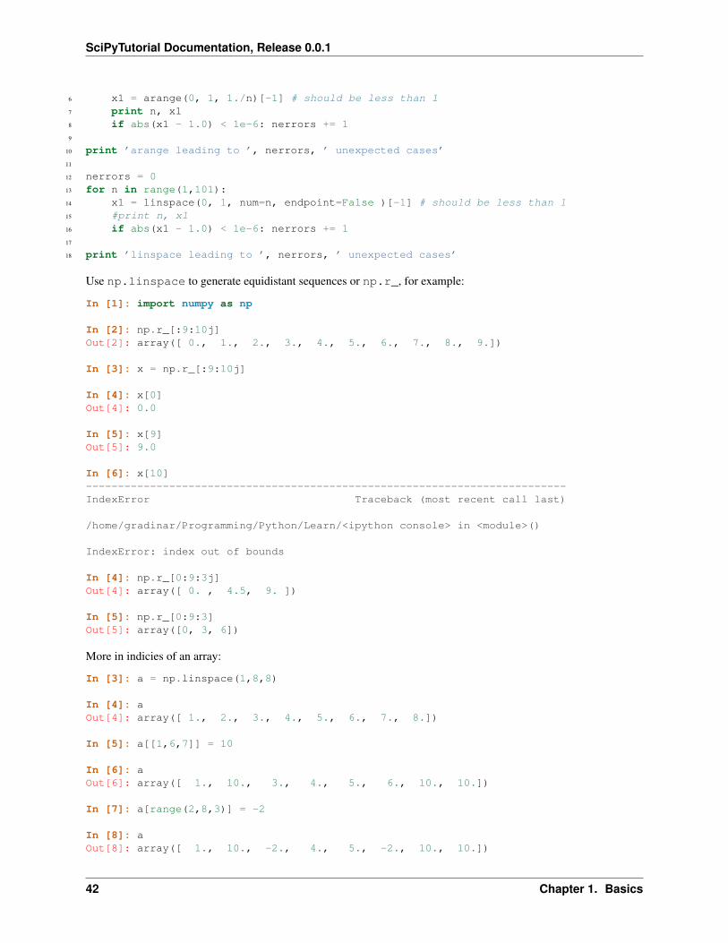
SciPyTutorial Documentation, Release 0.0.1
6 x1 = arange(0, 1, 1./n)[-1] # should be less than 17 print n, x18 if abs(x1 - 1.0) < 1e-6: nerrors += 19
10 print ’arange leading to ’, nerrors, ’ unexpected cases’11
12 nerrors = 013 for n in range(1,101):14 x1 = linspace(0, 1, num=n, endpoint=False )[-1] # should be less than 115 #print n, x116 if abs(x1 - 1.0) < 1e-6: nerrors += 117
18 print ’linspace leading to ’, nerrors, ’ unexpected cases’
Use np.linspace to generate equidistant sequences or np.r_, for example:
In [1]: import numpy as np
In [2]: np.r_[:9:10j]Out[2]: array([ 0., 1., 2., 3., 4., 5., 6., 7., 8., 9.])
In [3]: x = np.r_[:9:10j]
In [4]: x[0]Out[4]: 0.0
In [5]: x[9]Out[5]: 9.0
In [6]: x[10]---------------------------------------------------------------------------IndexError Traceback (most recent call last)
/home/gradinar/Programming/Python/Learn/<ipython console> in <module>()
IndexError: index out of bounds
In [4]: np.r_[0:9:3j]Out[4]: array([ 0. , 4.5, 9. ])
In [5]: np.r_[0:9:3]Out[5]: array([0, 3, 6])
More in indicies of an array:
In [3]: a = np.linspace(1,8,8)
In [4]: aOut[4]: array([ 1., 2., 3., 4., 5., 6., 7., 8.])
In [5]: a[[1,6,7]] = 10
In [6]: aOut[6]: array([ 1., 10., 3., 4., 5., 6., 10., 10.])
In [7]: a[range(2,8,3)] = -2
In [8]: aOut[8]: array([ 1., 10., -2., 4., 5., -2., 10., 10.])
42 Chapter 1. Basics
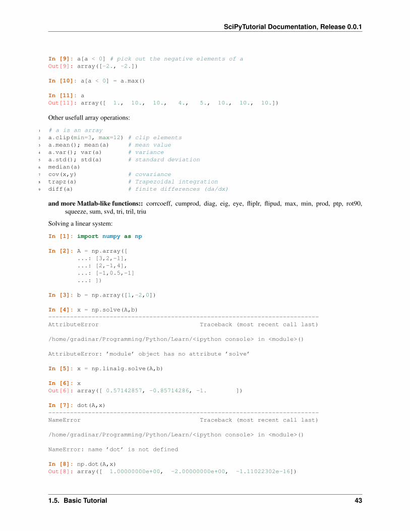
SciPyTutorial Documentation, Release 0.0.1
In [9]: a[a < 0] # pick out the negative elements of aOut[9]: array([-2., -2.])
In [10]: a[a < 0] = a.max()
In [11]: aOut[11]: array([ 1., 10., 10., 4., 5., 10., 10., 10.])
Other usefull array operations:
1 # a is an array2 a.clip(min=3, max=12) # clip elements3 a.mean(); mean(a) # mean value4 a.var(); var(a) # variance5 a.std(); std(a) # standard deviation6 median(a)7 cov(x,y) # covariance8 trapz(a) # Trapezoidal integration9 diff(a) # finite differences (da/dx)
and more Matlab-like functions:: corrcoeff, cumprod, diag, eig, eye, fliplr, flipud, max, min, prod, ptp, rot90,squeeze, sum, svd, tri, tril, triu
Solving a linear system:
In [1]: import numpy as np
In [2]: A = np.array([...: [3,2,-1],...: [2,-1,4],...: [-1,0.5,-1]...: ])
In [3]: b = np.array([1,-2,0])
In [4]: x = np.solve(A,b)---------------------------------------------------------------------------AttributeError Traceback (most recent call last)
/home/gradinar/Programming/Python/Learn/<ipython console> in <module>()
AttributeError: ’module’ object has no attribute ’solve’
In [5]: x = np.linalg.solve(A,b)
In [6]: xOut[6]: array([ 0.57142857, -0.85714286, -1. ])
In [7]: dot(A,x)---------------------------------------------------------------------------NameError Traceback (most recent call last)
/home/gradinar/Programming/Python/Learn/<ipython console> in <module>()
NameError: name ’dot’ is not defined
In [8]: np.dot(A,x)Out[8]: array([ 1.00000000e+00, -2.00000000e+00, -1.11022302e-16])
1.5. Basic Tutorial 43
SciPyTutorial Documentation, Release 0.0.1
In [9]: Ax = np.dot(A,x)
In [10]: np.allclose(Ax,b)Out[10]: True
Vectorization:
In [1]: import numpy as np
In [2]: def myfunc(x):...: if x >= 0: return x**2...: else: return -x...:...:
In [3]: myfunc(2)Out[3]: 4
In [5]: myfunc(np.array([-2,2]))---------------------------------------------------------------------------ValueError Traceback (most recent call last)
/home/gradinar/LaTeX_doc/Numcourses/Numcourses/SciPyTools/Start/<ipython console> in <module>()
/home/gradinar/LaTeX_doc/Numcourses/Numcourses/SciPyTools/Start/<ipython console> in myfunc(x)
ValueError: The truth value of an array with more than one element is ambiguous. Use a.any() or a.all()
In [6]: vecfunc = np.vectorize(myfunc, otypes=[float]) # it is important to declare the return type
In [8]: vecfunc(np.array([-2,2]))Out[8]: array([ 2., 4.])
In [9]: def myvecfunc(x):...: return np.where(x<0, -x, x**2)...:
In [10]: myvecfunc(np.array([-2,2]))Out[10]: array([2, 4])
NOTE that the hand written vectorization (last version) will run quicker than the automatically vectorized function.
• Simple Input/Output
• Professional I/O with HDF5
1.5.2 SciPy - Scientific tools for Python
SciPy is an Open Source library of scientific tools for Python. It depends on the NumPy library, and it gathers a varietyof high level science and engineering modules together as a single package. SciPy provides modules for
• statistics
• optimization
• numerical integration
• linear algebra
• Fourier transforms
44 Chapter 1. Basics
SciPyTutorial Documentation, Release 0.0.1
• signal processing
• image processing
• ODE solvers
• special functions
and more.
Root finding:
In [1]: coeffs = [1, -5, 6]
In [2]: import scipy as sp
In [3]: sp.roots(coeffs)Out[3]: array([ 3., 2.])
and now a more complicated function:
In [4]: from scipy.optimize import fsolve
In [5]: fsolve(sin(z)+cos(z)*cos(z),0)---------------------------------------------------------------------------NameError Traceback (most recent call last)
/home/gradinar/Programming/Python/Learn/<ipython console> in <module>()
NameError: name ’sin’ is not defined
In [6]: fsolve(sp.sin(z)+sp.cos(z)*sp.cos(z),0)---------------------------------------------------------------------------NameError Traceback (most recent call last)
/home/gradinar/Programming/Python/Learn/<ipython console> in <module>()
NameError: name ’z’ is not defined
In [7]: z = sp.linspace(-sp.i,sp.pi)---------------------------------------------------------------------------TypeError Traceback (most recent call last)
/home/gradinar/Programming/Python/Learn/<ipython console> in <module>()
TypeError: bad operand type for unary -: ’str’
In [8]: z = sp.linspace(-sp.pi,sp.pi)
In [9]: fsolve(sp.sin(z)+sp.cos(z)*sp.cos(z),0)---------------------------------------------------------------------------TypeError Traceback (most recent call last)
/home/gradinar/Programming/Python/Learn/<ipython console> in <module>()
/usr/lib64/python2.6/site-packages/scipy/optimize/minpack.pyc in fsolve(func, x0, args, fprime, full_output, col_deriv, xtol, maxfev, band, epsfcn, factor, diag, warning)111 n = len(x0)112 if type(args) != type(()): args = (args,)
--> 113 check_func(func,x0,args,n,(n,))114 Dfun = fprime115 if Dfun is None:
1.5. Basic Tutorial 45
SciPyTutorial Documentation, Release 0.0.1
/usr/lib64/python2.6/site-packages/scipy/optimize/minpack.pyc in check_func(thefunc, x0, args, numinputs, output_shape)1011 def check_func(thefunc, x0, args, numinputs, output_shape=None):
---> 12 res = atleast_1d(thefunc(*((x0[:numinputs],)+args)))13 if (output_shape is not None) and (shape(res) != output_shape):14 if (output_shape[0] != 1):
TypeError: ’numpy.ndarray’ object is not callable
In [10]: g = lambda z: sp.sin(z)+sp.cos(z)*sp.cos(z)
In [11]: g(0)Out[11]: 1.0
In [12]: fsolve(g,0)Out[12]: -0.66623943249251527
In [13]: from matplotlib import pyplot as plt
In [14]: plt.plot(z,g(z))Out[14]: [<matplotlib.lines.Line2D object at 0x7fd7ce10a9d0>]
In [15]: plt.show()
An example on least squares:
1 import scipy.linalg as splalg2 import scipy as sp3 from matplotlib import pyplot as plt4
5 n = 20 # sample length6 x = sp.linspace(0.,1.,n)7 y = -2*x+3 # line8 z = y + sp.random.normal(0.,0.25,n) # + noise9 A = sp.array([x, sp.ones(n)])
10 A = A.transpose()11 r = splalg.lstsq(A,z)12 # result is a 4-tuple, the solution (a,b) is the 1st entry13 a, b = r[0]14 plt.plot(x,z,’o’, x,y,’r’, x, a*x+b, ’b’)15 plt.legend((’data points’, ’original line’, ’fitted line’))16 plt.show()
46 Chapter 1. Basics
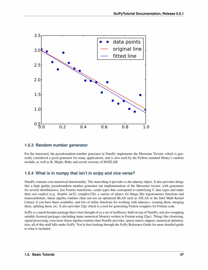
SciPyTutorial Documentation, Release 0.0.1
0.0 0.2 0.4 0.6 0.8 1.00.5
1.0
1.5
2.0
2.5
3.0
3.5
data pointsoriginal linefitted line
1.5.3 Random number generator
For the interested, the pseudorandom number generator in NumPy implements the Mersenne Twister, which is gen-erally considered a good generator for many applications, and is also used by the Python standard library’s randommodule, as well as R, Maple, Ruby and recent versions of MATLAB.
1.5.4 What is in numpy that isn’t in scipy and vice versa?
NumPy contains core numerical functionality. The main thing it provides is the ndarray object. It also provides thingslike a high quality pseudorandom number generator (an implementation of the Mersenne twister, with generatorsfor several distributions), fast Fourier transforms, scalar types that correspond to underlying C data types and maketheir size explicit (e.g. float64, int32, complex128), a variety of ufuncs for things like trigonometric functions andtranscendentals, linear algebra routines (that can use an optimized BLAS such as ATLAS or the Intel Math KernelLibrary if you have them available), and lots of utility functions for working with ndarrays: creating them, mergingthem, splitting them, etc. It also provides f2py which is a tool for generating Python wrappers for Fortran code.
SciPy is a much broader package that is best thought of as a set of toolboxes, built on top of NumPy, and also wrappingsuitably licensed packages (including many numerical libraries written in Fortran using f2py). Things like clustering,signal processing, even more linear algebra routines than NumPy provides, sparse matrix support, numerical optimiza-tion; all of this stuff falls under SciPy. You’re best looking through the SciPy Reference Guide for more detailed guideto what is included.
1.5. Basic Tutorial 47
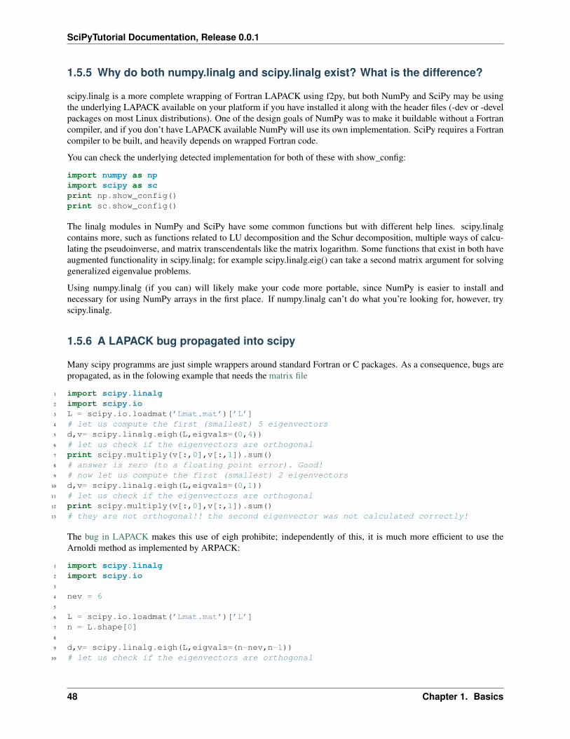
SciPyTutorial Documentation, Release 0.0.1
1.5.5 Why do both numpy.linalg and scipy.linalg exist? What is the difference?
scipy.linalg is a more complete wrapping of Fortran LAPACK using f2py, but both NumPy and SciPy may be usingthe underlying LAPACK available on your platform if you have installed it along with the header files (-dev or -develpackages on most Linux distributions). One of the design goals of NumPy was to make it buildable without a Fortrancompiler, and if you don’t have LAPACK available NumPy will use its own implementation. SciPy requires a Fortrancompiler to be built, and heavily depends on wrapped Fortran code.
You can check the underlying detected implementation for both of these with show_config:
import numpy as npimport scipy as scprint np.show_config()print sc.show_config()
The linalg modules in NumPy and SciPy have some common functions but with different help lines. scipy.linalgcontains more, such as functions related to LU decomposition and the Schur decomposition, multiple ways of calcu-lating the pseudoinverse, and matrix transcendentals like the matrix logarithm. Some functions that exist in both haveaugmented functionality in scipy.linalg; for example scipy.linalg.eig() can take a second matrix argument for solvinggeneralized eigenvalue problems.
Using numpy.linalg (if you can) will likely make your code more portable, since NumPy is easier to install andnecessary for using NumPy arrays in the first place. If numpy.linalg can’t do what you’re looking for, however, tryscipy.linalg.
1.5.6 A LAPACK bug propagated into scipy
Many scipy programms are just simple wrappers around standard Fortran or C packages. As a consequence, bugs arepropagated, as in the folowing example that needs the matrix file
1 import scipy.linalg2 import scipy.io3 L = scipy.io.loadmat(’Lmat.mat’)[’L’]4 # let us compute the first (smallest) 5 eigenvectors5 d,v= scipy.linalg.eigh(L,eigvals=(0,4))6 # let us check if the eigenvectors are orthogonal7 print scipy.multiply(v[:,0],v[:,1]).sum()8 # answer is zero (to a floating point error). Good!9 # now let us compute the first (smallest) 2 eigenvectors
10 d,v= scipy.linalg.eigh(L,eigvals=(0,1))11 # let us check if the eigenvectors are orthogonal12 print scipy.multiply(v[:,0],v[:,1]).sum()13 # they are not orthogonal!! the second eigenvector was not calculated correctly!
The bug in LAPACK makes this use of eigh prohibite; independently of this, it is much more efficient to use theArnoldi method as implemented by ARPACK:
1 import scipy.linalg2 import scipy.io3
4 nev = 65
6 L = scipy.io.loadmat(’Lmat.mat’)[’L’]7 n = L.shape[0]8
9 d,v= scipy.linalg.eigh(L,eigvals=(n-nev,n-1))10 # let us check if the eigenvectors are orthogonal
48 Chapter 1. Basics
SciPyTutorial Documentation, Release 0.0.1
11 print scipy.multiply(v[:,0],v[:,1]).sum()12
13 from scipy.sparse.linalg.eigen.arpack import arpack14 #from scipy.sparse.linalg.eigen.arpack import speigs15 from scipy.sparse import csr_matrix16
17 L = csr_matrix(L)18 #L = scipy.matrix(L)19 #L = L.tocsr()20
21
22 #da,va = arpack.eigen(L, k=nev)23 da,va = arpack.eigen_symmetric(L, k=nev)24 #da,va = speigs.ARPACK_eigs(L.matvec,n,nev, which=’LM’)25 va = scipy.matrix(va)26 print d27 I = abs(da).argsort()28 da.sort(); vac = va[:,I]29 print da30
31
32
33 print (vac.H*vac-scipy.eye(nev)).max()#scipy.multiply(v[:,0],v[:,1]).sum()34 #print ’eigh Arpack EV:’, v35 v = scipy.matrix(v)36 ve = v - vac37 #print v.shape, va.shape38 from scipy.linalg import norm39 print ve.shape40 z = scipy.array([norm(ve[:,k]) for k in xrange(nev)])41 print z42 #print z.max()43
44 #from scipy.sparse.linalg.eigen.arpack.arpack import eigen
1.5.7 Partial evaluation of functions
Assume you have a function of multiple arguments and already know some of them but not all. And you want orneed to bind the known parameters now. A common example is plotting of functions. Take the bessel functions, theyrequire an argument n which is the order (an integer in the most simple case) additionally the argument x. What canwe do now? Assume the plot command can not handle such functions. (In the example below we could just plug in theorder in the plot command, but there are other plot commands that only take the function object expecting somethinglike f(x).)
An example:
1 # Import bessel_j2 from scipy.special import jn3
4 # Evaluate J_n with n=2 at x=1.05 jn(2, 1.0)6 0.114903484931900497
8 # The partial evaluation tool9 from functools import partial
10
11 j = partial(jn, [2])
1.5. Basic Tutorial 49
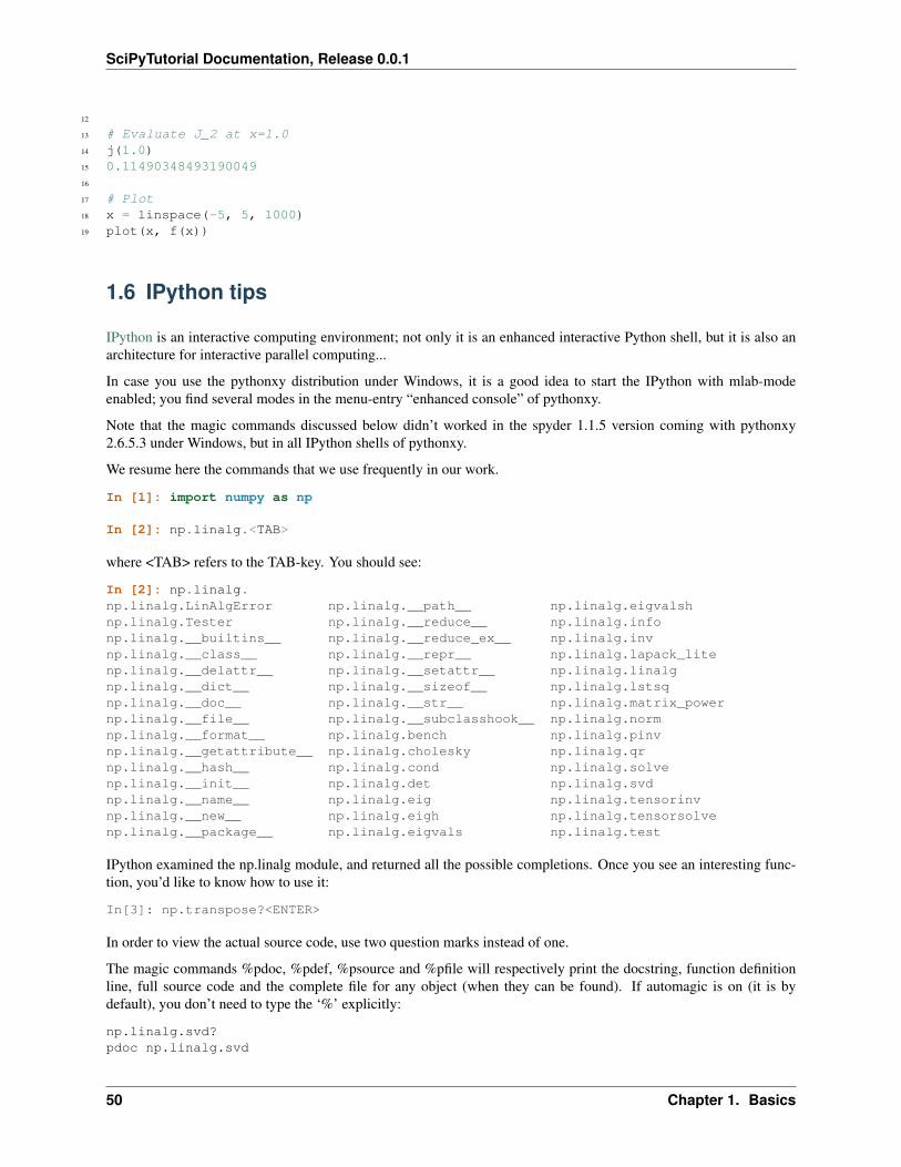
SciPyTutorial Documentation, Release 0.0.1
12
13 # Evaluate J_2 at x=1.014 j(1.0)15 0.1149034849319004916
17 # Plot18 x = linspace(-5, 5, 1000)19 plot(x, f(x))
1.6 IPython tips
IPython is an interactive computing environment; not only it is an enhanced interactive Python shell, but it is also anarchitecture for interactive parallel computing...
In case you use the pythonxy distribution under Windows, it is a good idea to start the IPython with mlab-modeenabled; you find several modes in the menu-entry “enhanced console” of pythonxy.
Note that the magic commands discussed below didn’t worked in the spyder 1.1.5 version coming with pythonxy2.6.5.3 under Windows, but in all IPython shells of pythonxy.
We resume here the commands that we use frequently in our work.
In [1]: import numpy as np
In [2]: np.linalg.<TAB>
where <TAB> refers to the TAB-key. You should see:
In [2]: np.linalg.np.linalg.LinAlgError np.linalg.__path__ np.linalg.eigvalshnp.linalg.Tester np.linalg.__reduce__ np.linalg.infonp.linalg.__builtins__ np.linalg.__reduce_ex__ np.linalg.invnp.linalg.__class__ np.linalg.__repr__ np.linalg.lapack_litenp.linalg.__delattr__ np.linalg.__setattr__ np.linalg.linalgnp.linalg.__dict__ np.linalg.__sizeof__ np.linalg.lstsqnp.linalg.__doc__ np.linalg.__str__ np.linalg.matrix_powernp.linalg.__file__ np.linalg.__subclasshook__ np.linalg.normnp.linalg.__format__ np.linalg.bench np.linalg.pinvnp.linalg.__getattribute__ np.linalg.cholesky np.linalg.qrnp.linalg.__hash__ np.linalg.cond np.linalg.solvenp.linalg.__init__ np.linalg.det np.linalg.svdnp.linalg.__name__ np.linalg.eig np.linalg.tensorinvnp.linalg.__new__ np.linalg.eigh np.linalg.tensorsolvenp.linalg.__package__ np.linalg.eigvals np.linalg.test
IPython examined the np.linalg module, and returned all the possible completions. Once you see an interesting func-tion, you’d like to know how to use it:
In[3]: np.transpose?<ENTER>
In order to view the actual source code, use two question marks instead of one.
The magic commands %pdoc, %pdef, %psource and %pfile will respectively print the docstring, function definitionline, full source code and the complete file for any object (when they can be found). If automagic is on (it is bydefault), you don’t need to type the ‘%’ explicitly:
np.linalg.svd?pdoc np.linalg.svd
50 Chapter 1. Basics
SciPyTutorial Documentation, Release 0.0.1
pdef np.linalg.svdpsource np.linalg.svd
Consider now the files sattelite.py that implements the simplified trajectory of a sattelite:
1 import numpy as np2 from matplotlib import pyplot as plt3
4 op = 2*np.pi; os = 14.*np.pi5 R = 4.; r = 0.256 t = np.linspace(0, 2, 2000)7 xp = np.cos(op*t)8 yp = np.sin(op*t)9 xs = xp + r*np.cos(os*t)
10 ys = yp + r*np.sin(os*t)11 plt.plot(xs,ys); plt.show()
Start IPython with the option -pylab:
ipython -pylabYour PyGtk has set_interactive(), so you can use themore stable single-threaded Gtk mode.See https://bugs.launchpad.net/ipython/+bug/270856Python 2.6.4 (r264:75706, Jul 14 2010, 09:36:06)Type "copyright", "credits" or "license" for more information.
IPython 0.10 -- An enhanced Interactive Python.? -> Introduction and overview of IPython’s features.%quickref -> Quick reference.help -> Python’s own help system.object? -> Details about ’object’. ?object also works, ?? prints more.
Welcome to pylab, a matplotlib-based Python environment.For more information, type ’help(pylab)’.
In [1]:
Now, we can use all functions implemented by pylab without importing them explicitly, a la Matlab. However, theprefferd style is to use:
from matplotlib import pyplot as plt
Exit by ^D(Ctrl-D)
The %run magic command:
run sattelite.pyrun -t sattelite.pyrun -p sattelite.pyrun -d sattelite.py
%run also has special flags for timing the execution of your scripts (-t) and for executing them under the controlof either Python’s pdb debugger (-d) or profiler (-p). With all of these, %run can be used as the main tool forefficient interactive development of code which you write in your editor of choice.
All output results are automatically stored in a global dictionary named Out and variables named _1, _2, etc. aliasthem. For example, the result of input line 4 is available either as Out[4] or as _4.
Put a ‘;’ at the end of a line to suppress the printing of output. The _* variables and the Out[] list do get updated withthe contents of the output, even if it is not printed. You can thus still access the generated results this way for further
1.6. IPython tips 51
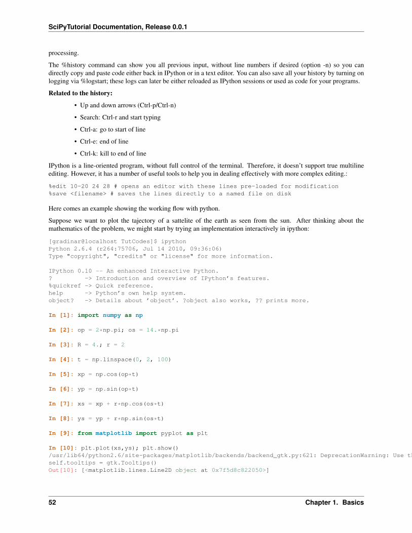
SciPyTutorial Documentation, Release 0.0.1
processing.
The %history command can show you all previous input, without line numbers if desired (option -n) so you candirectly copy and paste code either back in IPython or in a text editor. You can also save all your history by turning onlogging via %logstart; these logs can later be either reloaded as IPython sessions or used as code for your programs.
Related to the history:
• Up and down arrows (Ctrl-p/Ctrl-n)
• Search: Ctrl-r and start typing
• Ctrl-a: go to start of line
• Ctrl-e: end of line
• Ctrl-k: kill to end of line
IPython is a line-oriented program, without full control of the terminal. Therefore, it doesn’t support true multilineediting. However, it has a number of useful tools to help you in dealing effectively with more complex editing.:
%edit 10-20 24 28 # opens an editor with these lines pre-loaded for modification%save <filename> # saves the lines directly to a named file on disk
Here comes an example showing the working flow with python.
Suppose we want to plot the tajectory of a sattelite of the earth as seen from the sun. After thinking about themathematics of the problem, we might start by trying an implementation interactively in ipython:
[gradinar@localhost TutCodes]$ ipythonPython 2.6.4 (r264:75706, Jul 14 2010, 09:36:06)Type "copyright", "credits" or "license" for more information.
IPython 0.10 -- An enhanced Interactive Python.? -> Introduction and overview of IPython’s features.%quickref -> Quick reference.help -> Python’s own help system.object? -> Details about ’object’. ?object also works, ?? prints more.
In [1]: import numpy as np
In [2]: op = 2*np.pi; os = 14.*np.pi
In [3]: R = 4.; r = 2
In [4]: t = np.linspace(0, 2, 100)
In [5]: xp = np.cos(op*t)
In [6]: yp = np.sin(op*t)
In [7]: xs = xp + r*np.cos(os*t)
In [8]: ys = yp + r*np.sin(os*t)
In [9]: from matplotlib import pyplot as plt
In [10]: plt.plot(xs,ys); plt.show()/usr/lib64/python2.6/site-packages/matplotlib/backends/backend_gtk.py:621: DeprecationWarning: Use the new widget gtk.Tooltipself.tooltips = gtk.Tooltips()Out[10]: [<matplotlib.lines.Line2D object at 0x7f5d8c822050>]
52 Chapter 1. Basics
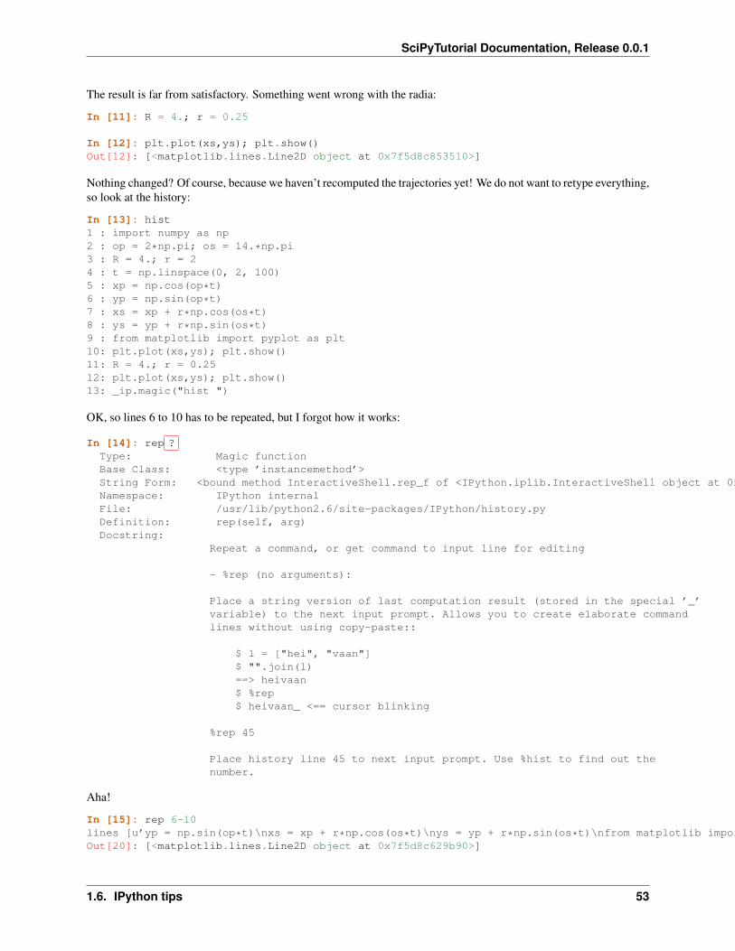
SciPyTutorial Documentation, Release 0.0.1
The result is far from satisfactory. Something went wrong with the radia:
In [11]: R = 4.; r = 0.25
In [12]: plt.plot(xs,ys); plt.show()Out[12]: [<matplotlib.lines.Line2D object at 0x7f5d8c853510>]
Nothing changed? Of course, because we haven’t recomputed the trajectories yet! We do not want to retype everything,so look at the history:
In [13]: hist1 : import numpy as np2 : op = 2*np.pi; os = 14.*np.pi3 : R = 4.; r = 24 : t = np.linspace(0, 2, 100)5 : xp = np.cos(op*t)6 : yp = np.sin(op*t)7 : xs = xp + r*np.cos(os*t)8 : ys = yp + r*np.sin(os*t)9 : from matplotlib import pyplot as plt10: plt.plot(xs,ys); plt.show()11: R = 4.; r = 0.2512: plt.plot(xs,ys); plt.show()13: _ip.magic("hist ")
OK, so lines 6 to 10 has to be repeated, but I forgot how it works:
In [14]: rep ?Type: Magic functionBase Class: <type ’instancemethod’>String Form: <bound method InteractiveShell.rep_f of <IPython.iplib.InteractiveShell object at 0x7f5da06a2d90>>Namespace: IPython internalFile: /usr/lib/python2.6/site-packages/IPython/history.pyDefinition: rep(self, arg)Docstring:
Repeat a command, or get command to input line for editing
- %rep (no arguments):
Place a string version of last computation result (stored in the special ’_’variable) to the next input prompt. Allows you to create elaborate commandlines without using copy-paste::
$ l = ["hei", "vaan"]$ "".join(l)==> heivaan$ %rep$ heivaan_ <== cursor blinking
%rep 45
Place history line 45 to next input prompt. Use %hist to find out thenumber.
Aha!
In [15]: rep 6-10lines [u’yp = np.sin(op*t)\nxs = xp + r*np.cos(os*t)\nys = yp + r*np.sin(os*t)\nfrom matplotlib import pyplot as plt\nplt.plot(xs,ys); plt.show()\n’]Out[20]: [<matplotlib.lines.Line2D object at 0x7f5d8c629b90>]
1.6. IPython tips 53
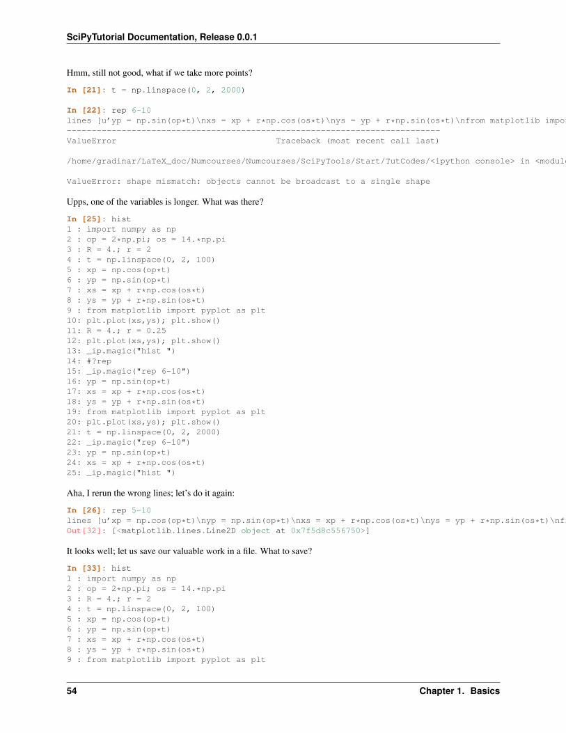
SciPyTutorial Documentation, Release 0.0.1
Hmm, still not good, what if we take more points?
In [21]: t = np.linspace(0, 2, 2000)
In [22]: rep 6-10lines [u’yp = np.sin(op*t)\nxs = xp + r*np.cos(os*t)\nys = yp + r*np.sin(os*t)\nfrom matplotlib import pyplot as plt\nplt.plot(xs,ys); plt.show()\n’]---------------------------------------------------------------------------ValueError Traceback (most recent call last)
/home/gradinar/LaTeX_doc/Numcourses/Numcourses/SciPyTools/Start/TutCodes/<ipython console> in <module>()
ValueError: shape mismatch: objects cannot be broadcast to a single shape
Upps, one of the variables is longer. What was there?
In [25]: hist1 : import numpy as np2 : op = 2*np.pi; os = 14.*np.pi3 : R = 4.; r = 24 : t = np.linspace(0, 2, 100)5 : xp = np.cos(op*t)6 : yp = np.sin(op*t)7 : xs = xp + r*np.cos(os*t)8 : ys = yp + r*np.sin(os*t)9 : from matplotlib import pyplot as plt10: plt.plot(xs,ys); plt.show()11: R = 4.; r = 0.2512: plt.plot(xs,ys); plt.show()13: _ip.magic("hist ")14: #?rep15: _ip.magic("rep 6-10")16: yp = np.sin(op*t)17: xs = xp + r*np.cos(os*t)18: ys = yp + r*np.sin(os*t)19: from matplotlib import pyplot as plt20: plt.plot(xs,ys); plt.show()21: t = np.linspace(0, 2, 2000)22: _ip.magic("rep 6-10")23: yp = np.sin(op*t)24: xs = xp + r*np.cos(os*t)25: _ip.magic("hist ")
Aha, I rerun the wrong lines; let’s do it again:
In [26]: rep 5-10lines [u’xp = np.cos(op*t)\nyp = np.sin(op*t)\nxs = xp + r*np.cos(os*t)\nys = yp + r*np.sin(os*t)\nfrom matplotlib import pyplot as plt\nplt.plot(xs,ys); plt.show()\n’]Out[32]: [<matplotlib.lines.Line2D object at 0x7f5d8c556750>]
It looks well; let us save our valuable work in a file. What to save?
In [33]: hist1 : import numpy as np2 : op = 2*np.pi; os = 14.*np.pi3 : R = 4.; r = 24 : t = np.linspace(0, 2, 100)5 : xp = np.cos(op*t)6 : yp = np.sin(op*t)7 : xs = xp + r*np.cos(os*t)8 : ys = yp + r*np.sin(os*t)9 : from matplotlib import pyplot as plt
54 Chapter 1. Basics
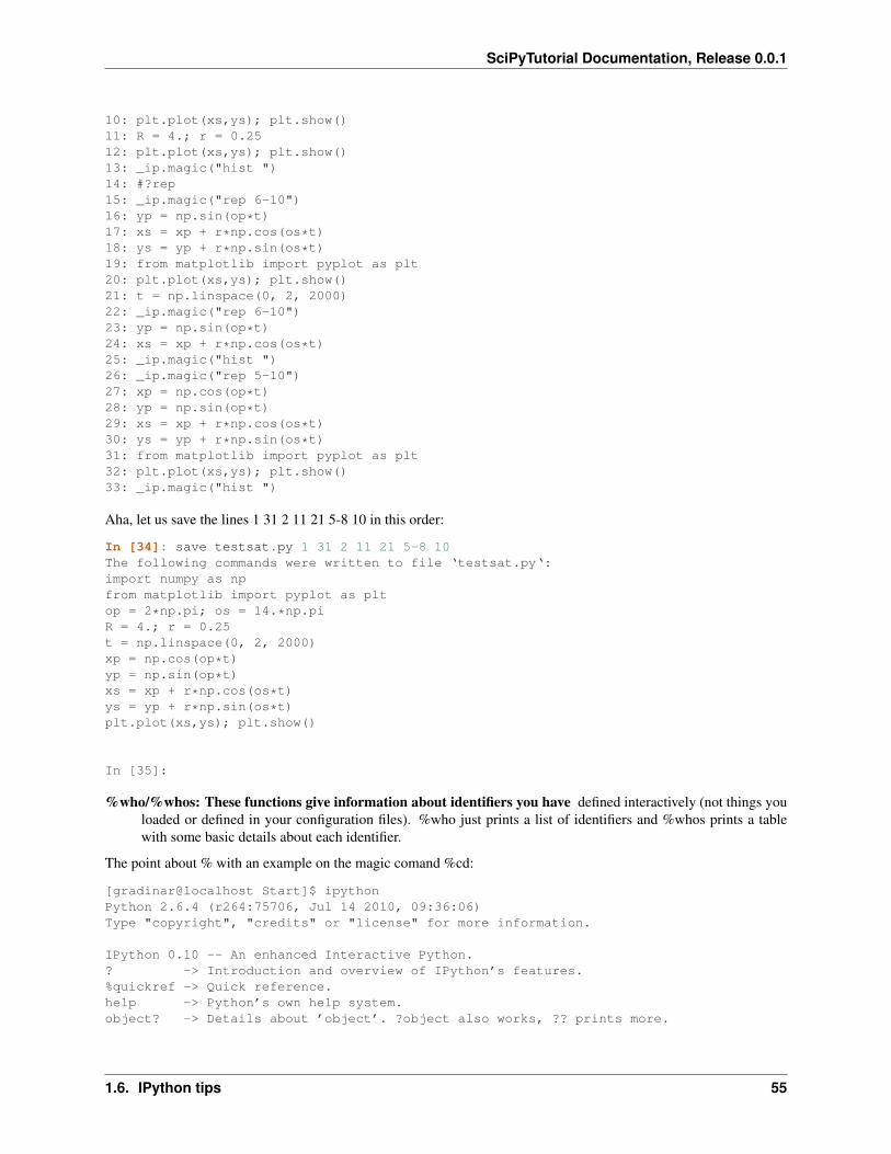
SciPyTutorial Documentation, Release 0.0.1
10: plt.plot(xs,ys); plt.show()11: R = 4.; r = 0.2512: plt.plot(xs,ys); plt.show()13: _ip.magic("hist ")14: #?rep15: _ip.magic("rep 6-10")16: yp = np.sin(op*t)17: xs = xp + r*np.cos(os*t)18: ys = yp + r*np.sin(os*t)19: from matplotlib import pyplot as plt20: plt.plot(xs,ys); plt.show()21: t = np.linspace(0, 2, 2000)22: _ip.magic("rep 6-10")23: yp = np.sin(op*t)24: xs = xp + r*np.cos(os*t)25: _ip.magic("hist ")26: _ip.magic("rep 5-10")27: xp = np.cos(op*t)28: yp = np.sin(op*t)29: xs = xp + r*np.cos(os*t)30: ys = yp + r*np.sin(os*t)31: from matplotlib import pyplot as plt32: plt.plot(xs,ys); plt.show()33: _ip.magic("hist ")
Aha, let us save the lines 1 31 2 11 21 5-8 10 in this order:
In [34]: save testsat.py 1 31 2 11 21 5-8 10The following commands were written to file ‘testsat.py‘:import numpy as npfrom matplotlib import pyplot as pltop = 2*np.pi; os = 14.*np.piR = 4.; r = 0.25t = np.linspace(0, 2, 2000)xp = np.cos(op*t)yp = np.sin(op*t)xs = xp + r*np.cos(os*t)ys = yp + r*np.sin(os*t)plt.plot(xs,ys); plt.show()
In [35]:
%who/%whos: These functions give information about identifiers you have defined interactively (not things youloaded or defined in your configuration files). %who just prints a list of identifiers and %whos prints a tablewith some basic details about each identifier.
The point about % with an example on the magic comand %cd:
[gradinar@localhost Start]$ ipythonPython 2.6.4 (r264:75706, Jul 14 2010, 09:36:06)Type "copyright", "credits" or "license" for more information.
IPython 0.10 -- An enhanced Interactive Python.? -> Introduction and overview of IPython’s features.%quickref -> Quick reference.help -> Python’s own help system.object? -> Details about ’object’. ?object also works, ?? prints more.
1.6. IPython tips 55
SciPyTutorial Documentation, Release 0.0.1
In [1]: cd ../home/gradinar/Documents/SciPyTutorial
In [2]: cd = 5
In [3]: cdOut[3]: 5
In [4]: cd Start------------------------------------------------------------File "<ipython console>", line 1
cd Start^
SyntaxError: invalid syntax
In [5]: %cd Start/home/gradinar/Documents/SciPyTutorial/Start
In [6]:
More nice documentation on IPython here.
1.7 Matplotlib tips
Matplotlib has a beautiful documentation.
You might start by the tutorial or by screen-shots
For special ploting wishes, look into the gallery, you might get either your ploting program already tipped or goodvisualization ideas.
1 import numpy as np2 from matplotlib import pyplot as plt3
4 # Data of the quadratic form5 A = np.array([6 [2., 1.],7 [1., 2.]8 ])9
10 b = np.array([1., 1.])11 # mesh12 Nx = 100; Ny = 10013 X,Y = np.ogrid[-3.:3:Nx*1j, -3.:3:Ny*1j]14 z = np.zeros(2)15 Z = np.zeros(Nx*Ny)16 # compute values17 k = 018 for x in X[:,0]:19 z[0] = x20 for y in Y[0,:]:21 z[1] = y22 Z[k] = 0.5*np.dot(z,np.dot(A,z)) - np.dot(z,b)23 k += 124
25 Z = Z.reshape(Nx,Ny)
56 Chapter 1. Basics
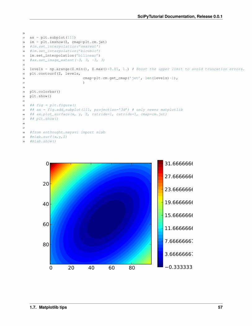
SciPyTutorial Documentation, Release 0.0.1
26
27 ax = plt.subplot(111)28 im = plt.imshow(Z, cmap=plt.cm.jet)29 #im.set_interpolation(’nearest’)30 #im.set_interpolation(’bicubic’)31 im.set_interpolation(’bilinear’)32 #ax.set_image_extent(-3, 3, -3, 3)33
34 levels = np.arange(Z.min(), Z.max()+0.01, 1.) # Boost the upper limit to avoid truncation errors.35 plt.contourf(Z, levels,36 cmap=plt.cm.get_cmap(’jet’, len(levels)-1),37 )38
39 plt.colorbar()40 plt.show()41
42 ## fig = plt.figure()43 ## ax = fig.add_subplot(111, projection=’3d’) # only newer matplotlib44 ## ax.plot_surface(x, y, Z, rstride=1, cstride=1, cmap=cm.jet)45 ## plt.show()46
47
48 #from enthought.mayavi import mlab49 #mlab.surf(x,y,Z)50 #mlab.show()
0 20 40 60 80
0
20
40
60
80
0.33333333
3.66666667
7.66666667
11.66666667
15.66666667
19.66666667
23.66666667
27.66666667
31.66666667
1.7. Matplotlib tips 57
SciPyTutorial Documentation, Release 0.0.1
1.7.1 TeX labels
The plotting utilities of matplotlib can use the power of a TeX system if one is installed. We just have to tell matplotlibthat it should generate the labels with the help of TeX. We then can use anything that is a valid TeX expression wewould otherwise write between the dollar signs in a TeX file. The following code presents a small example showingTeX labels in action.
NOTE: you may have issues with the following usetex-options in case that latex is bad configured on MacOS orWindows.
1 from numpy import *2 from pylab import *3 from matplotlib import rc4
5 # Enable usage of real TeX for labels and captions6 rc(’text’, usetex=True)7
8 # Build a complicated function9 x = linspace(-8, 8, 5000)
10
11 y = zeros(x.shape)12 for n in xrange(1,11,2):13 y += 1.0 / n * sin(n * pi * x / 6.0)14 y = pi / 4.0 * y15
16 # Plot and label with full TeX support17 figure()18 plot(x, y, label=r"$\frac{4}{\pi} \sum \frac{1}{n} \sin\left( \frac{n \pi x}{L} \right)$")19 xlabel(r"$\xi$")20 ylabel(r"$\mathcal{F}\left(f\left(x\right)\right)\left(\xi\right)$")21 legend(loc="lower right")22 title(r"Fourier series of a square wave: $\mathcal{F}\left(f\right) = \frac{4}{\pi} \sum_{n=1,3,5,\ldots} \frac{1}{n} \sin\left( \frac{n \pi x}{L} \right)$")23 savefig("tex_labels.png")
58 Chapter 1. Basics
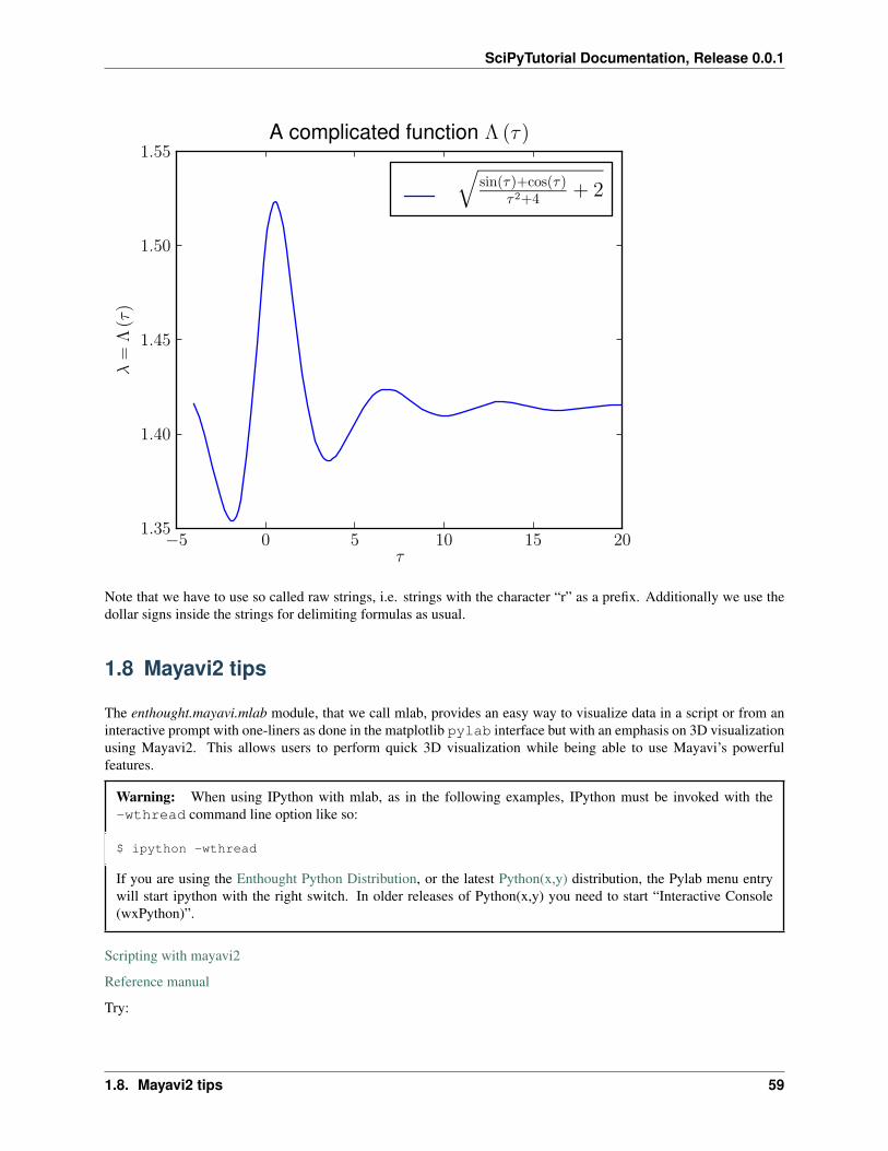
SciPyTutorial Documentation, Release 0.0.1
−5 0 5 10 15 20τ
1.35
1.40
1.45
1.50
1.55
λ=
Λ(τ
)A complicated function Λ (τ)
√sin(τ)+cos(τ)
τ2+4 + 2
Note that we have to use so called raw strings, i.e. strings with the character “r” as a prefix. Additionally we use thedollar signs inside the strings for delimiting formulas as usual.
1.8 Mayavi2 tips
The enthought.mayavi.mlab module, that we call mlab, provides an easy way to visualize data in a script or from aninteractive prompt with one-liners as done in the matplotlib pylab interface but with an emphasis on 3D visualizationusing Mayavi2. This allows users to perform quick 3D visualization while being able to use Mayavi’s powerfulfeatures.
Warning: When using IPython with mlab, as in the following examples, IPython must be invoked with the-wthread command line option like so:
$ ipython -wthread
If you are using the Enthought Python Distribution, or the latest Python(x,y) distribution, the Pylab menu entrywill start ipython with the right switch. In older releases of Python(x,y) you need to start “Interactive Console(wxPython)”.
Scripting with mayavi2
Reference manual
Try:
1.8. Mayavi2 tips 59
SciPyTutorial Documentation, Release 0.0.1
In [1]: from enthought.mayavi import mlab
In [2]: mlab.test_[TAB]
In [3]: mlab.test_contour3d ? ?
In [4]: mlab.test_contour3d()Out[4]: <enthought.mayavi.modules.iso_surface.IsoSurface object at 0x7fb8e8646b30>
In [5]: import numpy as np
In [6]: t = np.linspace(0, 2*np.pi, 50)
In [7]: u = np.cos(t)*np.pi
In [8]: x, y, z = np.sin(u), np.cos(u), np.sin(t)
In [9]: mlab.clf()
In [10]: mlab.points3d(x,y,z)
In [11]: mlab.clf()
In [12]: mlab.points3d(x,y,z,t, scale_mode=’none’)
In [13]: mlab.points3d ?
In [23]: x, y = np.mgrid[-3:3:100j, -3:3:100j ]
In [24]: z = np.sin(x*x + y*y)
In [25]: mlab.clf()
In [26]: mlab.surf(x,y,z)
In [28]: mlab.mesh(x,y,z)
A simple example showing a 3D plot done with the help of mayavi2. The following code shows what it takes toproduce such an image. The plotting is essentially only two lines of code!
1 from numpy import mgrid, real, conj, ones, zeros2 from numpy.fft.fftpack import fft23 from numpy.fft.helper import fftshift4 from enthought.mayavi import mlab5
6 # A mesh grid7 X,Y = mgrid[-100:100, -100:100]8
9 # The initial function: a 2D unit step10 Z = zeros((200,200))11 Z[0:6,0:6] = 0.3*ones((6,6))12
13 # The fourier transform: a 2D sinc(x,y)14 W = fftshift(fft2(Z))15 W = real(conj(W)*W)16
17 # Display the data with mayavi18 # Plot the original function
60 Chapter 1. Basics
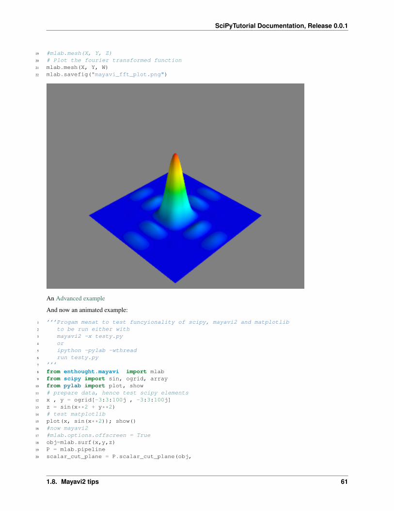
SciPyTutorial Documentation, Release 0.0.1
19 #mlab.mesh(X, Y, Z)20 # Plot the fourier transformed function21 mlab.mesh(X, Y, W)22 mlab.savefig("mayavi_fft_plot.png")
An Advanced example
And now an animated example:
1 ’’’Progam menat to test funcyionality of scipy, mayavi2 and matplotlib2 to be run either with3 mayavi2 -x testy.py4 or5 ipython -pylab -wthread6 run testy.py7 ’’’8 from enthought.mayavi import mlab9 from scipy import sin, ogrid, array
10 from pylab import plot, show11 # prepare data, hence test scipy elements12 x , y = ogrid[-3:3:100j , -3:3:100j]13 z = sin(x**2 + y**2)14 # test matplotlib15 plot(x, sin(x**2)); show()16 #now mayavi217 #mlab.options.offscreen = True18 obj=mlab.surf(x,y,z)19 P = mlab.pipeline20 scalar_cut_plane = P.scalar_cut_plane(obj,
1.8. Mayavi2 tips 61
SciPyTutorial Documentation, Release 0.0.1
21 plane_orientation=’y_axes’,22 )23 scalar_cut_plane.enable_contours = True24 scalar_cut_plane.contour.filled_contours = True25 scalar_cut_plane.implicit_plane.widget.origin = array([ 0.00000000e+00, 1.46059210e+00, -2.02655792e-06])26
27 scalar_cut_plane.warp_scalar.filter.normal = array([ 0., 1., 0.])28 scalar_cut_plane.implicit_plane.widget.normal = array([ 0., 1., 0.])29 ## mlab.draw()30 f = mlab.gcf()31 f.scene.camera.azimuth(10)32
33 f.scene.show_axes = True34 f.scene.magnification = 4 # or 435 mlab.axes()36 #engine=mlab.getengine()37 ## mlab.draw()38
39
40 # Now animate the data.41 dt = 0.01; N = 4042 ms = obj.mlab_source43 for k in xrange(N):44 x = x + k*dt45 scalars = sin(x**2 + y**2)46 ms.set(x=x, scalars=scalars)
The next example demonstrates how to use scalar cut planes in order to evidence subtle characteristics of a plot. Here,we would like to show the Gibbs oscillations in the Fourier series approximation of jumps.
The workflow for such a problem is:
• write a simple program (let us call it pl.py) that plots your object
• run mayavi2 -x pl.py (python pl.py works too for just executing the script)
• use the ‘spion’ of mayavi2: click on the red point in the menu: the protocol of everything you do visuallywith the mouse is python-scripted in the opened window
• play with the possibilities and variables that mayavi2 offers, till the image that you see satisfies yourexigences
• copy from the ‘spion’-window the relevant information for your result into your pl.py file
• save the picture, if you wish; CAUTION: the pictures that mayavi2 produces became huge, if saved invector graphics ... so eps is not recommeded here!
• re-run mayavi2 -x pl.py to see if this is really what you wanted
• iterate the above process, if wished
• improve speed and quality of the plot by avoiding rendering and increasing size
In the following code (that was developped following this receipt) you find hints for your formulations.
1 from numpy import mgrid, zeros, sin, pi, array2 from enthought.mayavi import mlab3
4 Lx = 45 Ly = 46
7 S = 10
62 Chapter 1. Basics
SciPyTutorial Documentation, Release 0.0.1
8 dx = 0.059 dy = 0.05
10
11 # A mesh grid12 X,Y = mgrid[-S:S:dx, -S:S:dy]13
14 # The initial function:15 #Z = zeros(X.shape)16 #Z = sin(pi*X/Lx)*sin(pi*Y/Ly)17 #Z[Z>0] = 118 #Z[Z<0] = -119
20 # The Fourier series:21 W = zeros(X.shape)22 m = 1023 for i in xrange(1,m,2):24 for j in xrange(1,m,2):25 W += 1.0 / (i*j) * sin(i * pi * X / Lx) * sin(j * pi * Y / Ly)26 W *= pi / 4.027
28
29 # prepare scene30 scene = mlab.gcf()31 # next two lines came at the very end of the design32 scene.scene.off_screen_rendering = True # quicker execution because no redenring33 scene.scene.magnification = 434 # plot the object !35 obj = mlab.mesh(X, Y, W)36 P = mlab.pipeline37 # first scalar_cut_plane38 scalar_cut_plane = P.scalar_cut_plane(obj,39 plane_orientation=’z_axes’,40 )41 scalar_cut_plane.enable_contours = True42 scalar_cut_plane.contour.filled_contours = True43 # where ?44 scalar_cut_plane.implicit_plane.widget.origin = array([-0.025, -0.025, 0.48])45 scalar_cut_plane.warp_scalar.filter.normal = array([ 0., 0., 1.])46 scalar_cut_plane.implicit_plane.widget.normal = array([ 0., 0., 1.])47 scalar_cut_plane.implicit_plane.widget.enabled = False # do not show the widget48 # second scalar_cut-plane49 scalar_cut_plane_2 = P.scalar_cut_plane(obj,50 plane_orientation=’z_axes’,51 )52 scalar_cut_plane_2.enable_contours = True53 scalar_cut_plane_2.contour.filled_contours = True54 # where ?55 scalar_cut_plane_2.implicit_plane.widget.origin = array([-0.025, -0.025, -0.48])56 scalar_cut_plane_2.warp_scalar.filter.normal = array([ 0., 0., 1.])57 scalar_cut_plane_2.implicit_plane.widget.normal = array([ 0., 0., 1.])58 scalar_cut_plane_2.implicit_plane.widget.enabled = False # do not show the widget59 # see it from a closer view point60 scene.scene.camera.position = [-31.339891336951567, 14.405281950904936, -27.156389988308661]61 scene.scene.camera.focal_point = [-0.025000095367431641, -0.025000095367431641, 0.0]62 scene.scene.camera.view_angle = 30.063 scene.scene.camera.view_up = [0.63072643330371414, -0.083217283169475589, -0.77153033000256477]64 scene.scene.camera.clipping_range = [4.7116394000124906, 93.313165745624019]65 scene.scene.camera.compute_view_plane_normal()
1.8. Mayavi2 tips 63
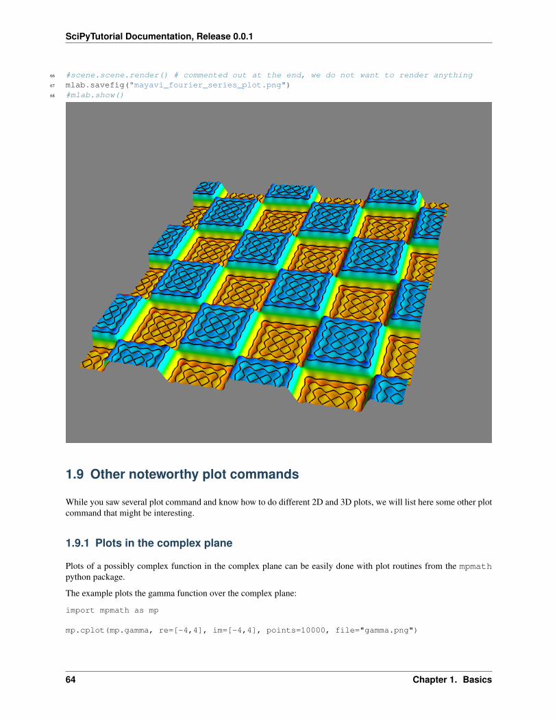
SciPyTutorial Documentation, Release 0.0.1
66 #scene.scene.render() # commented out at the end, we do not want to render anything67 mlab.savefig("mayavi_fourier_series_plot.png")68 #mlab.show()
1.9 Other noteworthy plot commands
While you saw several plot command and know how to do different 2D and 3D plots, we will list here some other plotcommand that might be interesting.
1.9.1 Plots in the complex plane
Plots of a possibly complex function in the complex plane can be easily done with plot routines from the mpmathpython package.
The example plots the gamma function over the complex plane:
import mpmath as mp
mp.cplot(mp.gamma, re=[-4,4], im=[-4,4], points=10000, file="gamma.png")
64 Chapter 1. Basics
SciPyTutorial Documentation, Release 0.0.1
This is all for plotting the gamma function in the rectangle -4 < Re(z) < 4 and -4 < Im(z) < 4. The above call saves theresult to the file “gamma.png” which looks like this:
1.10 Examples
Here we put a few complete examples that should be relevant for the numerics lectures.
1.10.1 First example
Define f(x) = 1√1−a sin(2πx−1)
.
We want to plot the error made by using the trapezoidal rule when approximating∫ 1
0f(x)dx and
∫ 0.5
0f(x)dx.
.
As exact value we take the value of the integral as produced by the function quad from the sub-package integrate ofscipy. This function is just a wrapper to the Fortran library QUADPACK. Please, use IPython facility to consult thedocumentation of it.
The aim of the plots is to put in evidence the exponential convergence of the trapezoidal rule when the smoothness ofthe function extends above its periodical domain. The plots should be done for several possible parameters 0 < a < 1.
1 import numpy as np2 import matplotlib.pyplot as plt3 from scipy import integrate4
5 def trapr(func, a, b, N):6 #h = (b-a)/N; x = np.arange(a, b + h, h)7 x = np.linspace(a,b, N+1); h = x[1]-x[0]8 res = np.sum(func(x[1:-1])) + 0.5*(func(x[0])+func(x[-1]))9 res *= h
10 return res11
12 N = 25 #number of quadrature points used13 res = np.zeros(N) # alocate space for results14 left = 0.; right = 1. # integration limits15
16 lista = [0.5, 0.9, 0.95, 0.99]17 for a in lista:18 myf = lambda x: 1./np.sqrt(1.- a*np.sin(2*np.pi*x-1))19 for n in xrange(N):20 res[n] = trapr(myf, left, right, n+1)21 exact, aerr = integrate.quad(myf, left, right)22 #exact = trapr(myf, left, right, 500)23 print ’a=’,a,’quad:’, exact, ’aerr=’, aerr24 err = np.abs(res-exact)25 plt.semilogy(np.arange(1,N+1),err, label=’a=’+str(a))26
27 plt.legend(loc=0)28 plt.show()
1.10. Examples 65
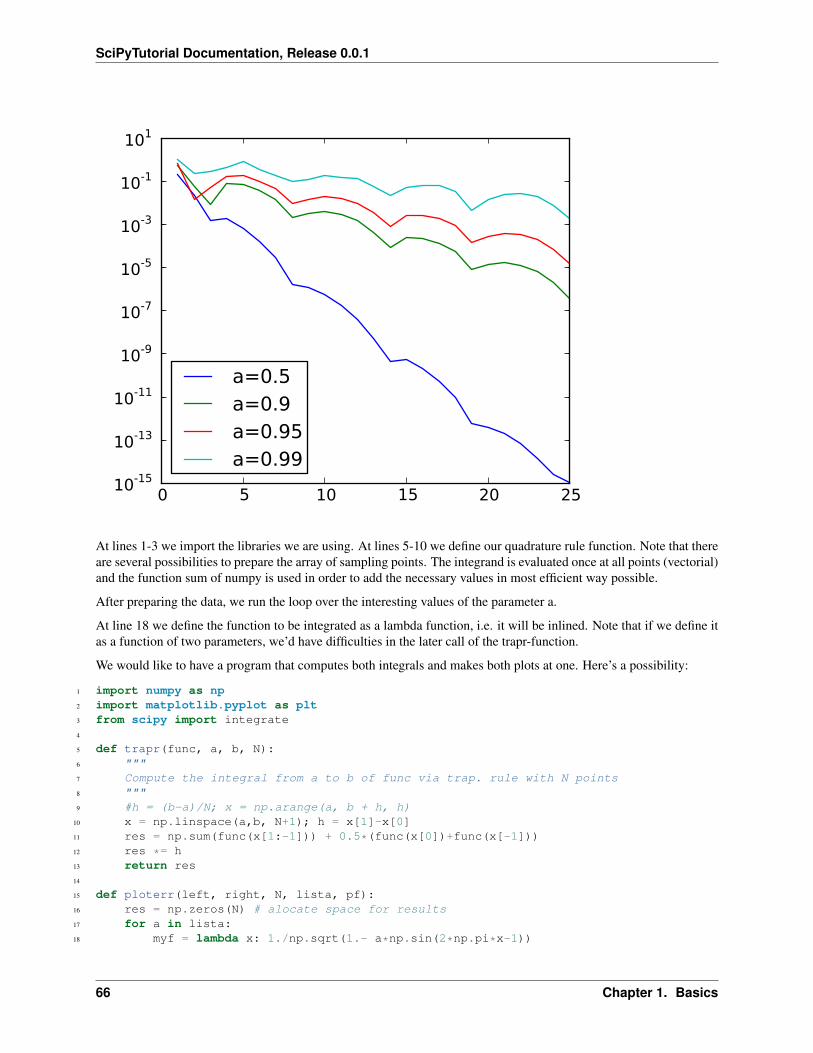
SciPyTutorial Documentation, Release 0.0.1
0 5 10 15 20 2510-15
10-13
10-11
10-9
10-7
10-5
10-3
10-1
101
a=0.5a=0.9a=0.95a=0.99
At lines 1-3 we import the libraries we are using. At lines 5-10 we define our quadrature rule function. Note that thereare several possibilities to prepare the array of sampling points. The integrand is evaluated once at all points (vectorial)and the function sum of numpy is used in order to add the necessary values in most efficient way possible.
After preparing the data, we run the loop over the interesting values of the parameter a.
At line 18 we define the function to be integrated as a lambda function, i.e. it will be inlined. Note that if we define itas a function of two parameters, we’d have difficulties in the later call of the trapr-function.
We would like to have a program that computes both integrals and makes both plots at one. Here’s a possibility:
1 import numpy as np2 import matplotlib.pyplot as plt3 from scipy import integrate4
5 def trapr(func, a, b, N):6 """7 Compute the integral from a to b of func via trap. rule with N points8 """9 #h = (b-a)/N; x = np.arange(a, b + h, h)
10 x = np.linspace(a,b, N+1); h = x[1]-x[0]11 res = np.sum(func(x[1:-1])) + 0.5*(func(x[0])+func(x[-1]))12 res *= h13 return res14
15 def ploterr(left, right, N, lista, pf):16 res = np.zeros(N) # alocate space for results17 for a in lista:18 myf = lambda x: 1./np.sqrt(1.- a*np.sin(2*np.pi*x-1))
66 Chapter 1. Basics
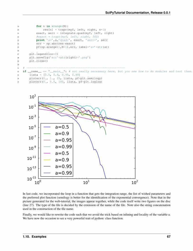
SciPyTutorial Documentation, Release 0.0.1
19 for n in xrange(N):20 res[n] = trapr(myf, left, right, n+1)21 exact, aerr = integrate.quad(myf, left, right)22 #exact = trapr(myf, left, right, 500)23 print ’a=’,a,’quad:’, exact, ’aerr=’, aerr24 err = np.abs(res-exact)25 pf(np.arange(1,N+1),err, label=’a=’+str(a))26
27 plt.legend(loc=0)28 plt.savefig(’err’+str(right)+’.png’)29 plt.close()30
31 # ----------------------------------------------------------32 if __name__ == "__main__": # not really necessary here, but you see how to do modules and test them...33 lista = [0.5, 0.9, 0.95, 0.99]34 ploterr(0., 1., 25, lista, pf=plt.semilogy)35 ploterr(0., 0.5, 100, lista, pf=plt.loglog)
100 101 10210-15
10-13
10-11
10-9
10-7
10-5
10-3
10-1
101
a=0.5a=0.9a=0.95a=0.99a=0.5a=0.9a=0.95a=0.99
In last code, we incorporated the loop in a function that gets the integration range, the list of wished parameters andthe preferred plot function (semilogy is better for the identification of the exponential convergence). Note that in thepicture generated for the web-tutorial, the images appear together, while the code itself write two figures on the disc(line 27). The type of the file is decided by the extension of the name of the file. Note also the string concatenationused in the construction of the file name.
Finally, we would like to rewrite the code such that we avoid the trick based on inlining and locality of the variable a.We have now the occasion to see a very powerful trait of python: class function.
1.10. Examples 67
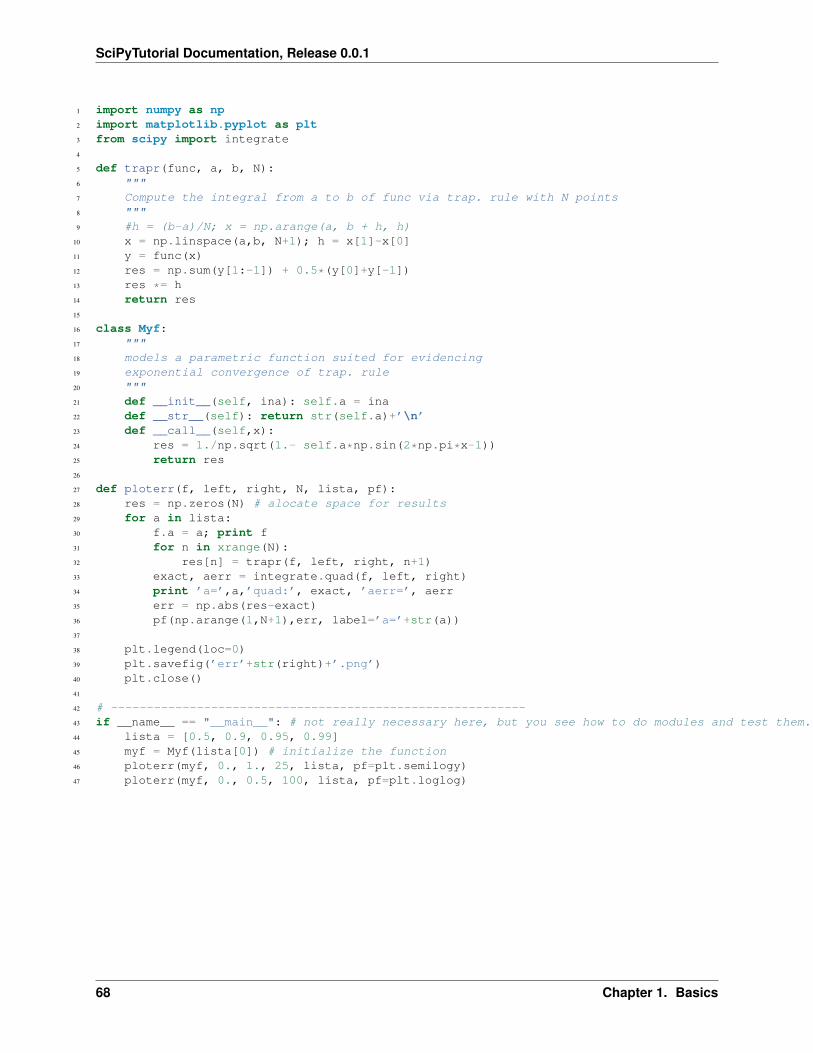
SciPyTutorial Documentation, Release 0.0.1
1 import numpy as np2 import matplotlib.pyplot as plt3 from scipy import integrate4
5 def trapr(func, a, b, N):6 """7 Compute the integral from a to b of func via trap. rule with N points8 """9 #h = (b-a)/N; x = np.arange(a, b + h, h)
10 x = np.linspace(a,b, N+1); h = x[1]-x[0]11 y = func(x)12 res = np.sum(y[1:-1]) + 0.5*(y[0]+y[-1])13 res *= h14 return res15
16 class Myf:17 """18 models a parametric function suited for evidencing19 exponential convergence of trap. rule20 """21 def __init__(self, ina): self.a = ina22 def __str__(self): return str(self.a)+’\n’23 def __call__(self,x):24 res = 1./np.sqrt(1.- self.a*np.sin(2*np.pi*x-1))25 return res26
27 def ploterr(f, left, right, N, lista, pf):28 res = np.zeros(N) # alocate space for results29 for a in lista:30 f.a = a; print f31 for n in xrange(N):32 res[n] = trapr(f, left, right, n+1)33 exact, aerr = integrate.quad(f, left, right)34 print ’a=’,a,’quad:’, exact, ’aerr=’, aerr35 err = np.abs(res-exact)36 pf(np.arange(1,N+1),err, label=’a=’+str(a))37
38 plt.legend(loc=0)39 plt.savefig(’err’+str(right)+’.png’)40 plt.close()41
42 # ----------------------------------------------------------43 if __name__ == "__main__": # not really necessary here, but you see how to do modules and test them...44 lista = [0.5, 0.9, 0.95, 0.99]45 myf = Myf(lista[0]) # initialize the function46 ploterr(myf, 0., 1., 25, lista, pf=plt.semilogy)47 ploterr(myf, 0., 0.5, 100, lista, pf=plt.loglog)
68 Chapter 1. Basics
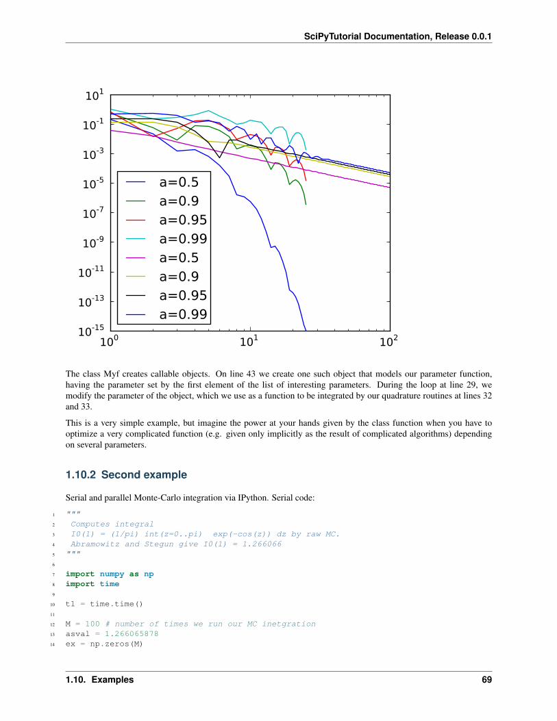
SciPyTutorial Documentation, Release 0.0.1
100 101 10210-15
10-13
10-11
10-9
10-7
10-5
10-3
10-1
101
a=0.5a=0.9a=0.95a=0.99a=0.5a=0.9a=0.95a=0.99
The class Myf creates callable objects. On line 43 we create one such object that models our parameter function,having the parameter set by the first element of the list of interesting parameters. During the loop at line 29, wemodify the parameter of the object, which we use as a function to be integrated by our quadrature routines at lines 32and 33.
This is a very simple example, but imagine the power at your hands given by the class function when you have tooptimize a very complicated function (e.g. given only implicitly as the result of complicated algorithms) dependingon several parameters.
1.10.2 Second example
Serial and parallel Monte-Carlo integration via IPython. Serial code:
1 """2 Computes integral3 I0(1) = (1/pi) int(z=0..pi) exp(-cos(z)) dz by raw MC.4 Abramowitz and Stegun give I0(1) = 1.2660665 """6
7 import numpy as np8 import time9
10 t1 = time.time()11
12 M = 100 # number of times we run our MC inetgration13 asval = 1.26606587814 ex = np.zeros(M)
1.10. Examples 69
SciPyTutorial Documentation, Release 0.0.1
15 print ’A and S tables: I0(1) = ’,asval16 print ’sample variance MC I0 val’17 print ’------ -------- ---------’18 k = 5 # how many experiments19 N = 10**np.arange(1,k+1)20 v = []; e = []21 for n in N:22 for m in xrange(M):23 x = np.random.rand(n) # sample24 x = np.exp(np.cos(-np.pi*x))25 ex[m] = sum(x)/n # quadrature26 ev = sum(ex)/M27 vex = np.dot(ex,ex)/M28 vex -= ev**229 v += [vex]; e += [ev]30 print n, vex, ev31
32 t2 = time.time()33 t = t2-t134
35 print "Serial calculation completed, time = %s s" % t
Parallel code:
1 import sys2 import time3 from IPython.kernel import client4 import numpy as np5 from matplotlib import pyplot as plt6
7
8 def mcquad():9 k = 5 # how many experiments
10 N = 10**np.arange(1,k+1)11 ex = []12 for n in N:13 x = np.random.rand(n) # sample14 x = np.exp(np.cos(-np.pi*x))15 ex += [np.sum(x)/n] # quadrature16 return ex17
18 #-----------------------------------------------------------------------------19 # Setup for parallel calculation20 #-----------------------------------------------------------------------------21
22 # The MultiEngineClient is used to setup the calculation and works with all23 # engine.24 mec = client.MultiEngineClient()25
26 # The TaskClient is an interface to the engines that provides dynamic load27 # balancing at the expense of not knowing which engine will execute the code.28 tc = client.TaskClient()29
30 # Initialize the common code on the engines.31 mec.execute(’import numpy as np’)32
33
34 #-----------------------------------------------------------------------------
70 Chapter 1. Basics
SciPyTutorial Documentation, Release 0.0.1
35 # Perform parallel calculation36 #-----------------------------------------------------------------------------37
38 print "Running parallel calculation"39 M = 100 # number of times we run our MC inetgration40
41 # Submit tasks to the TaskClient for each N as a MapTask.42 t1 = time.time()43 taskids = []44 for m in xrange(M):45 t = client.MapTask(46 mcquad47 )48 taskids.append(tc.run(t))49
50 print "Submitted tasks: ", len(taskids)51 sys.stdout.flush()52
53 # Block until all tasks are completed.54 tc.barrier(taskids)55 t2 = time.time()56 t = t2-t157
58 print "Parallel calculation completed, time = %s s" % t59 print "Collecting results..."60
61 # Get the results using TaskClient.get_task_result.62 results = [tc.get_task_result(tid) for tid in taskids]63 ex = np.array(results)64 ev = ex.sum(axis=0)/M65 vex = (ex**2).sum(axis=0)/M66 vex = vex - ev**267 print vex
To use the parallel code, start first an IPython controller with:
gradinar@cmath-2% ipcluster local -n 4
then open a new window on the same machine and start ipython:
gradinar@cmath-2% ipythonPython 2.6.4 (r264:75706, Jun 4 2010, 18:20:31)Type "copyright", "credits" or "license" for more information.
IPython 0.10 -- An enhanced Interactive Python.? -> Introduction and overview of IPython’s features.%quickref -> Quick reference.help -> Python’s own help system.object? -> Details about ’object’. ?object also works, ?? prints more.
In [1]: run -i par01.pyclass FCTaskControllerFromTaskController(Referenceable):Running parallel calculationSubmitted tasks: 100Parallel calculation completed, time = 1.54661202431 sCollecting results...[ 6.04508921e-02 6.88178837e-03 7.46274110e-04 6.50926168e-05 5.63334832e-06]
More on Using IPython for parallel computing
1.10. Examples 71
SciPyTutorial Documentation, Release 0.0.1
1.10.3 Third example
1 """2 Calculates eigenvalues through direct power method3
4 Originaly, there were the input parameters d and maxit,5 but in the skript, d = [1:10]’ and maxit = 30 are used.6 """7
8 import numpy as np9
10 def pm(A,z,sgn,ev,ew,maxit=30):11 ’’’12 performs maxit iterations of the power method13 for the matrix A and the initial vector z14 and computes the error for the largest eigenvalue ew15 having the sign sgn and the corresponding eigenvector ev16 ’’’17 res = np.zeros((maxit,5))18 s = 1;19 for k in xrange(maxit):20 w = np.dot(A,z)21 no = np.linalg.norm(w)22 rq = np.real(np.vdot(w,z))23 z = w/no24 err_aew = abs(no-abs(ew))25 err_ew = abs(sgn*rq-ew)26 err_ev = np.linalg.norm(s*z-ev)27 res[k] = np.array([k, no, err_ev, err_aew, err_ew])28 s = s*sgn29 return res30
31 def runpm(d, fname):32 ’’’33 performs the analysis of the power iteration starting from34 the array of eigenvalues d; the picture with the results goes35 to the file indicate by fname36 ’’’37 n = len(d) # size of the matrix38 S = np.triu(np.diag(np.r_[n:0:-1]) + np.ones((n,n)))39 A = np.dot(S, np.dot(np.diag(d), np.linalg.inv(S)) )40 # need exact ew and ew for error calculation41 w, V = np.linalg.eig(A)42 t = np.where(w == abs(w).max())43 k = t[0];44 if len(k) > 1:45 print ’Error: no single larges EV’46 raise ValueError47 ev = V[:,k[0]]; ev /= np.linalg.norm(ev)48 ew = w[k[0]]49 ## # another way to do this is:50 ## t = (w == abs(w).max()) # array of booleans showing where w ==max(|w|)51 ## if t.sum()>1:52 ## print ’Error: no single larges EV’53 ## raise ValueError54 ## k = t.argmax()55 ## ev = V[:,k]; ev /= np.linalg.norm(ev)56 ## ew = w[k]
72 Chapter 1. Basics
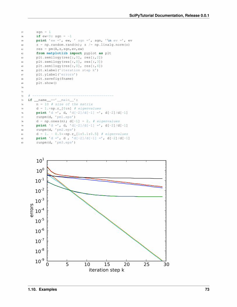
SciPyTutorial Documentation, Release 0.0.1
57 sgn = 158 if ew<0: sgn = -159 print ’ew =’, ew, ’ sgn =’, sgn, ’\n ev =’, ev60 z = np.random.rand(n); z /= np.linalg.norm(z)61 res = pm(A,z,sgn,ev,ew)62 from matplotlib import pyplot as plt63 plt.semilogy(res[:,0], res[:,2])64 plt.semilogy(res[:,0], res[:,3])65 plt.semilogy(res[:,0], res[:,4])66 plt.xlabel(’iteration step k’)67 plt.ylabel(’errors’)68 plt.savefig(fname)69 plt.show()70
71
72 # ---------------------------------------73 if __name__==’__main__’:74 n = 10 # size of the matrix75 d = 1.+np.r_[0:n] # eigenvalues76 print ’d =’, d, ’d[-2]/d[-1] =’, d[-2]/d[-1]77 runpm(d, ’pm1.eps’)78 d = np.ones(n); d[-1] = 2. # eigenvalues79 print ’d =’, d, ’d[-2]/d[-1] =’, d[-2]/d[-1]80 runpm(d, ’pm2.eps’)81 d = 1. - 0.5**np.r_[1:5.1:0.5] # eigenvalues82 print ’d =’, d , ’d[-2]/d[-1] =’, d[-2]/d[-1]83 runpm(d, ’pm3.eps’)
0 5 10 15 20 25 30iteration step k
10-9
10-8
10-7
10-6
10-5
10-4
10-3
10-2
10-1
100
101
err
ors
1.10. Examples 73
SciPyTutorial Documentation, Release 0.0.1
1.11 Useful links
1.11.1 Tutorials, Manuals and Books
• Tentative NumPy Tutorial
• NumPy for Matlab Users
• Documentations on NumPy and SciPy
• Additional documentation from SciPy
• Scipy tutorial
• Kittens tutorial
• SciPy FAQ page
• NumPy
• Short NumPy introduction
• IPython documentation.
• SymPy documentation
• h5py project website and h5py user guide
• Ask scipy page
• A very good book on the subject is H. Langtangen, “Python Scripting for Computational Science”, availableelectronically on NEBIS, too.
• A very good French overview
1.11.2 Local copies at a given moment:
• Tentative NumPy Tutorial
• NumPy for Matlab Users
• Numpy 1.3 Reference Guide [HTML+zip]
• Scipy 0.7 Reference Guide [HTML+zip]
• French overview
1.11.3 Additional software
• The spyder IDE
• winpdb, a python debugger
• mayavi2, 3D scientific data visualization
• image magic, batch image processing
• mplayer, versatile video player and encoder
• hdfview, HDF file editor
74 Chapter 1. Basics
SciPyTutorial Documentation, Release 0.0.1
1.12 Installing python packages
There are thousands of python packages available 2 and not all of them can be found in the package repositories ofthe common Linux distributions. Even if Debian for example consists of over 30‘000 software packages, there arepython packages that are not part of the Debian distribution. For this reason you need to install python packages byhand sometimes. This is not a difficult task but you have to obey some constraints.
If you download a python package, it’s usually an archive file in the .zip or .tar.gz format. Within this archivethere is a file called setup.py, this acts as an installer. (For more information about the topis, see the officialdocumentation on the Distutils python module 3.)
Installing the python package locally on your Linux system is as easy as running the setup.py script with theargument install. (Uninstalling works similar, but we don’t go into details here.):
python setup.py install
This tries to install the package on a system-wide basis. If you do not have the permissions to do this or you just wantto try a new package quickly, then it’s preferable to install the package only locally. Assume you want to install it in~/my_python/. Then you first create that directory:
cd ~mkdir my_python
and then tell the setup script where to install the package:
python setup.py install --home=~/my_python/
that’s it. But you can not import the new module yet.
The installation directory lies outside of the so called python path where python searches for referenced modules.(This is similar to how the shell searches for binaries in the directories listed in the variable $PATH.) To resolve thisissue you just have to prepend the new directory path to the $PYTHONPATH variable:
export PYTHONPATH="~/my_python/lib/python:$PYTHONPATH"
where the part lib/python/ is the exact path to the python module. You can put this last line of shell code intoyour ~/.bashrc file to avoid the need of manually executing it every time you want to use the new python module.
2 Python Package Index http://pypi.python.org/pypi.3 For more information on how to distribute python software see http://docs.python.org/distutils/index.html.
1.12. Installing python packages 75

SciPyTutorial Documentation, Release 0.0.1
76 Chapter 1. Basics
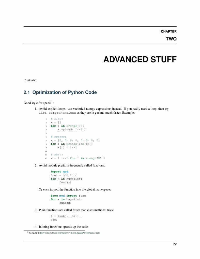
CHAPTER
TWO
ADVANCED STUFF
Contents:
2.1 Optimization of Python Code
Good style for speed 1:
1. Avoid explicit loops: use vectorizd numpy expressions instead. If you really need a loop, then trylist comprehensions as they are in general much faster. Example:
1 # Slow:2 x = []3 for i in xrange(8):4 x.append( i**2 )5
6 # Better:7 x = [0, 0, 0, 0, 0, 0, 0, 0]8 for i in xrange(len(x)):9 x[i] = i**2
10
11 # Best:12 x = [ i**2 for i in xrange(8) ]
2. Avoid module prefix in frequently called funcions:
import modfunc = mod.funcfor x in hugelist:
func(x)
Or even import the function into the global namespace:
from mod import funcfor x in hugelist:
func(x)
3. Plain functions are called faster than class methods: trick:
f = myobj.__call__f(x)
4. Inlining functions speeds-up the code
1 See also http://wiki.python.org/moin/PythonSpeed/PerformanceTips
77
SciPyTutorial Documentation, Release 0.0.1
5. Avoid usieng numpy functions with scalar arguments
6. Use xrange instead of range (but be aware that xrange only supports a small part of the interface ofrange() and similar containers. 2)
7. if-else is faster than try-except (never use exceptions for program flow!)
8. Avoid resizing of numpy arrays
9. Callbacks to Python from Fortran/C/C++ are expensive
10. Avoid unnecessary allocation of large data structures
11. Be careful with type mactching in mixed Python-Fortran software (e.g. flat/ real*8): if the array entrytypes do not match, arrays will be copied!
12. Use asarray with parameter order=’Fortran’ when sending arrays from numpy to Fortran routines!
2.2 Timing Your Code
Timing your code is a more complex task you imagine. If the code to run takes long and you are not fond in veryprecise measurements, then the module time is a very simple way to do it. Otherwise you should use the moduletimeit. See the two examples below.
from numpy import r_, mat, vstack, eye, ones, zerosfrom scipy.linalg import qrimport timenrEXP = 4sizes = 2**r_[2:6]qrtimes = zeros((5,sizes.shape[0]))k = 0for n in sizes:
print ’n=’, nm = n**2A = mat(1.*r_[1:m+1]).T*mat(1.*r_[1:n+1])A += vstack((eye(n), ones((m-n,n)) ))avqr = 0.for k in xrange(nrEXP):
t1 = time.clock()Q, R = qr(A)t2 = time.clock()-t1avqr += t2
avqr /= nrEXPprint avqrqrtimes[0,k] = avqravqr = 0.for k in xrange(nrEXP):
t1 = time.clock()Q, R = qr(A, econ=True)t2 = time.clock()-t1avqr += t2
avqr /= nrEXPprint avqr
2 Objects of type xrange don’t support slicing, concatenation or repetition, xrange objects have very little behavior: they only support indexing,iteration, and the len() function. The advantage of the xrange type is that an xrange object will always take the same amount of memory, no matterthe size of the range it represents. (This is some kind of lazy evaluation.) http://docs.python.org/library/functions.html#xrange
78 Chapter 2. Advanced Stuff
SciPyTutorial Documentation, Release 0.0.1
qrtimes[1,k] = avqravqr = 0.for k in xrange(nrEXP):
t1 = time.clock()Q, R = qr(A, econ=True, overwrite_a=True)t2 = time.clock()-t1avqr += t2
avqr /= nrEXPprint avqrqrtimes[2,k] = avqravqr = 0.for k in xrange(nrEXP):
t1 = time.clock()R = qr(A, mode=’r’)t2 = time.clock()-t1avqr += t2
avqr /= nrEXPprint avqrqrtimes[3,k] = avqravqr = 0.for k in xrange(nrEXP):
t1 = time.clock()R = qr(A, mode=’r’, econ=True)t2 = time.clock()-t1avqr += t2
avqr /= nrEXPprint avqrqrtimes[4,k] = avqrk += 1
import matplotlib.pyplot as pltplt.loglog(sizes, qrtimes[0], label=’qr’)plt.loglog(sizes, qrtimes[1], label="qr(econ=True)")plt.loglog(sizes, qrtimes[2], label="qr(econ=True, overwrite_a=True)")plt.loglog(sizes, qrtimes[3], label="qr(mode=’r’)")plt.loglog(sizes, qrtimes[4], label="qr(mode=’r’, econ=True)")#plt.legend()plt.show()
2.2. Timing Your Code 79
SciPyTutorial Documentation, Release 0.0.1
100 101 10210-3
10-2
10-1
100
from numpy import r_, mat, vstack, eye, ones, zerosfrom scipy.linalg import qrimport timeit
def qr_full():global AQ, R = qr(A)
def qr_econ():global AQ, R = qr(A, econ=True)
def qr_ovecon():global AQ, R = qr(A, econ=True, overwrite_a=True)
def qr_r():global AR = qr(A, mode=’r’)
def qr_recon():global AR = qr(A, mode=’r’, econ=True)
nrEXP = 4sizes = 2**r_[2:6]qrtimes = zeros((5,sizes.shape[0]))k = 0
80 Chapter 2. Advanced Stuff
SciPyTutorial Documentation, Release 0.0.1
for n in sizes:print ’n=’, nm = n**2#4*nA = mat(1.*r_[1:m+1]).T*mat(1.*r_[1:n+1])A += vstack((eye(n), ones((m-n,n)) ))
t = timeit.Timer(’qr_full()’,’from __main__ import qr_full’)avqr = t.timeit(number=nrEXP)/nrEXPprint avqrqrtimes[0,k] = avqr
t = timeit.Timer(’qr_econ()’,’from __main__ import qr_econ’)avqr = t.timeit(number=nrEXP)/nrEXPprint avqrqrtimes[1,k] = avqr
t = timeit.Timer(’qr_ovecon()’,’from __main__ import qr_ovecon’)avqr = t.timeit(number=nrEXP)/nrEXPprint avqrqrtimes[2,k] = avqr
t = timeit.Timer(’qr_r()’,’from __main__ import qr_r’)avqr = t.timeit(number=nrEXP)/nrEXPprint avqrqrtimes[3,k] = avqr
t = timeit.Timer(’qr_recon()’,’from __main__ import qr_recon’)avqr = t.timeit(number=nrEXP)/nrEXPprint avqrqrtimes[4,k] = avqr
k += 1
#print qrtimes[3]import matplotlib.pyplot as pltplt.loglog(sizes, qrtimes[0], ’s’, label=’qr’)plt.loglog(sizes, qrtimes[1], ’*’, label="qr(econ=True)")plt.loglog(sizes, qrtimes[2], ’.’, label="qr(econ=True, overwrite_a=True)")plt.loglog(sizes, qrtimes[3], ’o’, label="qr(mode=’r’)")plt.loglog(sizes, qrtimes[4], ’+’, label="qr(mode=’r’, econ=True)")v4 = qrtimes[1,1]* (sizes/sizes[1])**4v6 = qrtimes[0,1]* (sizes/sizes[1])**6plt.loglog(sizes, v4, label=’$O(n^4)$’)plt.loglog(sizes, v6, ’--’,label=’$O(n^6)$’)#plt.legend(loc=2)plt.xlabel(’$n$’)plt.ylabel(’time [s]’)#plt.savefig(’qrtiming.eps’)plt.show()
2.2. Timing Your Code 81
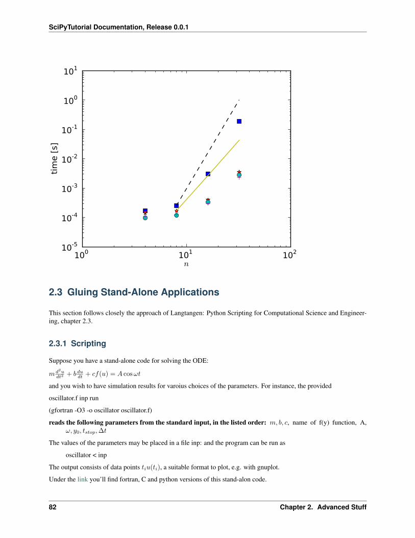
SciPyTutorial Documentation, Release 0.0.1
100 101 102
n
10-5
10-4
10-3
10-2
10-1
100
101
tim
e [
s]
2.3 Gluing Stand-Alone Applications
This section follows closely the approach of Langtangen: Python Scripting for Computational Science and Engineer-ing, chapter 2.3.
2.3.1 Scripting
Suppose you have a stand-alone code for solving the ODE:
md2udt2 + bdudt + cf(u) = A cos ωt
and you wish to have simulation results for varoius choices of the parameters. For instance, the provided
oscillator.f inp run
(gfortran -O3 -o oscillator oscillator.f)
reads the following parameters from the standard input, in the listed order: m, b, c, name of f(y) function, A,ω, y0, tstop, ∆t
The values of the parameters may be placed in a file inp: and the program can be run as
oscillator < inp
The output consists of data points tiu(ti), a suitable format to plot, e.g. with gnuplot.
Under the link you’ll find fortran, C and python versions of this stand-alon code.
82 Chapter 2. Advanced Stuff
SciPyTutorial Documentation, Release 0.0.1
Our first goal is to simplify the user’s interaction with the program; with the script simviz1.py it is possible to adjustthe parameters through command-line options:
python simviz1.py -m 3.3 -b 0.9 -dt 0.05
The result should be png-files and an otional plot on the screen. The files for each such experiment should go in asubdirectory.
1 #!/usr/bin/env python2 import sys, math3
4 # default values of input parameters:5 m = 1.0; b = 0.7; c = 5.0; func = ’y’; A = 5.0; w = 2*math.pi6 y0 = 0.2; tstop = 30.0; dt = 0.05; case = ’tmp1’; screenplot = 17
8 # read variables from the command line, one by one:9 while len(sys.argv) > 1:
10 option = sys.argv[1]; del sys.argv[1]11 if option == ’-m’:12 m = float(sys.argv[1]); del sys.argv[1]13 elif option == ’-b’:14 b = float(sys.argv[1]); del sys.argv[1]15 elif option == ’-c’:16 c = float(sys.argv[1]); del sys.argv[1]17 elif option == ’-func’:18 func = sys.argv[1]; del sys.argv[1]19 elif option == ’-A’:20 A = float(sys.argv[1]); del sys.argv[1]21 elif option == ’-w’:22 w = float(sys.argv[1]); del sys.argv[1]23 elif option == ’-y0’:24 y0 = float(sys.argv[1]); del sys.argv[1]25 elif option == ’-tstop’:26 tstop = float(sys.argv[1]); del sys.argv[1]27 elif option == ’-dt’:28 dt = float(sys.argv[1]); del sys.argv[1]29 elif option == ’-noscreenplot’:30 screenplot = 031 elif option == ’-case’:32 case = sys.argv[1]; del sys.argv[1]33 else:34 print sys.argv[0],’: invalid option’,option35 sys.exit(1)36
37 # create a subdirectory:38 d = case # name of subdirectory39 import os, shutil40 if os.path.isdir(d): # does d exist?41 shutil.rmtree(d) # yes, remove old directory42 os.mkdir(d) # make new directory d43 os.chdir(d) # move to new directory d44
45 # make input file to the program:46 f = open(’%s.i’ % case, ’w’)47 # write a multi-line (triple-quoted) string with48 # variable interpolation:49 f.write("""50 %(m)g51 %(b)g
2.3. Gluing Stand-Alone Applications 83
SciPyTutorial Documentation, Release 0.0.1
52 %(c)g53 %(func)s54 %(A)g55 %(w)g56 %(y0)g57 %(tstop)g58 %(dt)g59 """ % vars())60 f.close()61 # run simulator:62 cmd = ’../oscillator < %s.i’ % case # command to run63 failure = os.system(cmd)64 if failure:65 print ’running the oscillator code failed’; sys.exit(1)66
67 # make file with gnuplot commands:68 f = open(case + ’.gnuplot’, ’w’)69 f.write("""70 set title ’%s: m=%g b=%g c=%g f(y)=%s A=%g w=%g y0=%g dt=%g’;71 """ % (case, m, b, c, func, A, w, y0, dt))72 if screenplot:73 f.write("plot ’sim.dat’ title ’y(t)’ with lines;\n")74 f.write("""75 set size ratio 0.3 1.5, 1.0;76 # define the postscript output format:77 set term postscript eps monochrome dashed ’Times-Roman’ 28;78 # output file containing the plot:79 set output ’%s.ps’;80 # basic plot command:81 plot ’sim.dat’ title ’y(t)’ with lines;82 # make a plot in PNG format:83 set term png small;84 set output ’%s.png’;85 plot ’sim.dat’ title ’y(t)’ with lines;86 """ % (case, case))87 f.close()88 # make plot:89 cmd = ’gnuplot -geometry 800x200 -persist ’ + case + ’.gnuplot’90 failure = os.system(cmd)91 if failure:92 print ’running gnuplot failed’; sys.exit(1)
One can easily generate an automatic LaTeX-report or HTML-report containing the values of the parameters and thecorresponding pictures.
2.3.2 Conducting Numerical Experiments
Suppose we want to keep most of the parameters fixed and vary one parameter between a minimum and a maximumvalue; the results should be collected in a HTML-report:
python loop4simviz1.py m_min m_max m_increment [ simviz1.py options ]
1 #!/usr/bin/env python2 """calls simviz1.py with different m values (in a loop)"""3 import sys, os4 usage = ’Usage: %s m_min m_max m_increment [ simviz1.py options ]’ \5 % sys.argv[0]
84 Chapter 2. Advanced Stuff
SciPyTutorial Documentation, Release 0.0.1
6
7 try:8 m_min = float(sys.argv[1])9 m_max = float(sys.argv[2])
10 dm = float(sys.argv[3])11 except IndexError:12 print usage; sys.exit(1)13
14 simviz1_options = ’ ’.join(sys.argv[4:])15
16 html = open(’tmp_mruns.html’, ’w’)17 html.write(’<HTML><BODY BGCOLOR="white">\n’)18 psfiles = [] # plot files in PostScript format19
20 m = m_min21 while m <= m_max:22 case = ’tmp_m_%g’ % m23 cmd = ’python simviz1.py %s -m %g -case %s’ % \24 (simviz1_options, m, case)25 print ’running’, cmd26 os.system(cmd)27 html.write(’<H1>m=%g</H1> <IMG SRC="%s">\n’ \28 % (m,os.path.join(case,case+’.png’)))29 psfiles.append(os.path.join(case,case+’.ps’))30 m += dm31 html.write(’</BODY></HTML>\n’)
or let vary any parameter:
loop4simviz2.py parameter min max increment [ simviz2.py options ]
1 #!/usr/bin/env python2 """3 As loop4simviz1.py, but here we call simviz2.py, make movies,4 and also allow any simviz2.py option to be varied in a loop.5 """6 import sys, os7 usage = ’Usage: %s parameter min max increment ’\8 ’[ simviz2.py options ]’ % sys.argv[0]9 try:
10 option_name = sys.argv[1]11 min = float(sys.argv[2])12 max = float(sys.argv[3])13 incr = float(sys.argv[4])14 except:15 print usage; sys.exit(1)16
17 simviz2_options = ’ ’.join(sys.argv[5:])18
19 html = open(’tmp_%s_runs.html’ % option_name, ’w’)20 html.write(’<HTML><BODY BGCOLOR="white">\n’)21 psfiles = [] # plot files in PostScript format22 pngfiles = [] # plot files in PNG format23
24 value = min25 while value <= max:26 case = ’tmp_%s_%g’ % (option_name,value)27 cmd = ’python simviz2.py %s -%s %g -case %s’ % \28 (simviz2_options, option_name, value, case)
2.3. Gluing Stand-Alone Applications 85
SciPyTutorial Documentation, Release 0.0.1
29 print ’running’, cmd30 os.system(cmd)31 psfile = os.path.join(case,case+’.ps’)32 pngfile = os.path.join(case,case+’.png’)33 html.write(’<H1>%s=%g</H1> <IMG SRC="%s">\n’ \34 % (option_name, value, pngfile))35 psfiles.append(psfile)36 pngfiles.append(pngfile)37 value += incr38 cmd = ’convert -delay 50 -loop 1000 %s tmp_%s.gif’ \39 % (’ ’.join(pngfiles), option_name)40 print ’converting PNG files to animated GIF:\n’, cmd41 os.system(cmd)42 html.write(’<H1>Movie</H1> <IMG SRC="tmp_%s.gif">\n’ % option_name)43 html.write(’</BODY></HTML>\n’)44 html.close()
2.4 Symbolical calculations
Even if we want to deal with numerical computations mainly, I’d like to give a short introduction into symboliccalculation. There are several reasons why we want to include some symbolic manipulations in a numerical code. Forexample we want to do an error analysis and would like to be able to evaluate the known exact solution on variousdifferent grids. Or we have a closed form solution for some right hand side. Beyond the toy examples there exist alsoindustrial strength codes that use symbolic computation in a preparation step before going into the numerics 3.
In any case, we could put the symbolic expression literally into the source code. But sometimes it would be useful ifwe could do a few more things with the expression beside numerical evaluation, for example we may need the firstderivative. The benefit of symbolic calculation is now that we can compute this derivation without explicitly put it intothe source code or falling back to numerical techniques.
In the following section I’ll show a really simple example of how to use the power of the sympy python module. Thismodule acts as a library for symbolic calculation and is quite easy to use yet surprisingly powerful for it’s complexity.
1 # Use explicit namespaces to make clear from which package a function comes.2 import sympy as sp3 import numpy as np4 import pylab as pl5
6 # Define a symbol7 x = sp.Symbol("x")8
9 # A symbolic expression10 expr = sp.sin(x) + x**211
12 # We can evaluate it for any value of x:13 print(expr({x:sp.pi**2}))14
15
16 # A function for evaluating the expression by symbolic17 # manipulations. We have to assign the function parameter18 # y to the symbolic variable x of the expression.19 fs = lambda y: expr({x:y})20
21 # Again we can evaluate the expression for any value of x easily:
3 See fore example SyFi which is part of the FEniCS project: http://www.fenicsproject.org/wiki/FEniCS_Project
86 Chapter 2. Advanced Stuff
SciPyTutorial Documentation, Release 0.0.1
22 print(fs(2))23 print(fs(sp.pi))24
25
26 # But we want the function to work with the arrays from numpy too.27 # Thus we have to lambdify the expression.28 fn = sp.lambdify(x, expr, "numpy")29
30 xvals = np.linspace(-5,5,100)31 yvals = fn(xvals)32
33
34 # Compute the derivative of our expression35 dexpr = sp.diff(expr, x)36
37 # And again lambdify it38 fnd = sp.lambdify(x, dexpr, "numpy")39
40 # Evaluate the derivative on the given grid41 dyvals = fnd(xvals)42
43
44 # Compute the second derivative of our expression45 ddexpr = sp.diff(expr, x, 2)46
47 # And again lambdify it48 fndd = sp.lambdify(x, ddexpr, "numpy")49
50 # Evaluate the derivative on the given grid51 ddyvals = fndd(xvals)52
53
54 # And plot the function sampled at the grid points xvals55 # Note how we reuse the symbolic expressions for generating the plot labels too!56 pl.figure()57 pl.plot(xvals, yvals, label=sp.latex(expr))58 pl.plot(xvals, dyvals, label=sp.latex(dexpr))59 pl.plot(xvals, ddyvals, label=sp.latex(ddexpr))60 pl.legend()61 pl.savefig("symbolics_demo.png")
And this is how the output looks like
2.4. Symbolical calculations 87
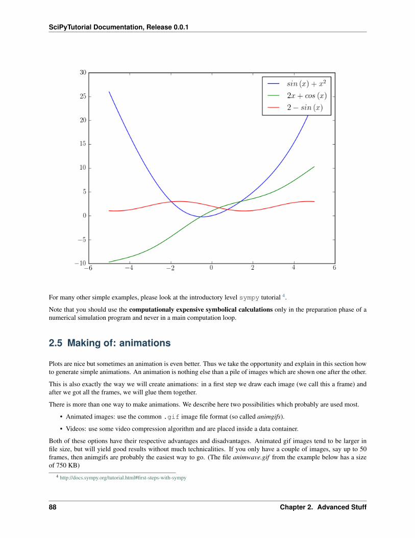
SciPyTutorial Documentation, Release 0.0.1
For many other simple examples, please look at the introductory level sympy tutorial 4.
Note that you should use the computationaly expensive symbolical calculations only in the preparation phase of anumerical simulation program and never in a main computation loop.
2.5 Making of: animations
Plots are nice but sometimes an animation is even better. Thus we take the opportunity and explain in this section howto generate simple animations. An animation is nothing else than a pile of images which are shown one after the other.
This is also exactly the way we will create animations: in a first step we draw each image (we call this a frame) andafter we got all the frames, we will glue them together.
There is more than one way to make animations. We describe here two possibilities which probably are used most.
• Animated images: use the common .gif image file format (so called animgifs).
• Videos: use some video compression algorithm and are placed inside a data container.
Both of these options have their respective advantages and disadvantages. Animated gif images tend to be larger infile size, but will yield good results without much technicalities. If you only have a couple of images, say up to 50frames, then animgifs are probably the easiest way to go. (The file animwave.gif from the example below has a sizeof 750 KB)
4 http://docs.sympy.org/tutorial.html#first-steps-with-sympy
88 Chapter 2. Advanced Stuff
SciPyTutorial Documentation, Release 0.0.1
For longer animations you should of course use the advantages of modern video compression techniques. But maturevideo encoding tools usually have a huge number of options interacting in a complex manner. It’s not easy to find theparameters which give you the best result. For example the video compression algorithms are tuned for areas and canintroduce bad artefacts if the image has only a bunch sharp lines in front of a uniform background. But this is whatplots look like most of the time! (By the way, the file animwave.flv from the example below has a size of 700 KB.)
2.5.1 External tools
We additionaly need two programs which are not part of the python installation as proposed at the beginning of thistutorial. But they may be already preinstalled on a common Linux system today.
The first of these tools is called convertwhich is itself part of the well known ImageMagic batch image processor.We use this tool for creating animated gif images.
• ImageMagic can be found at http://www.imagemagick.org/
(This is not the only tool that can compose gif files, you may also try gifsicle which can be found athttp://www.lcdf.org/gifsicle/. My own experience is that this tool sometimes is faster, uses less memory and theresulting files are smaller in size. But don’t take this as a given.)
To encode videos we use the famous mplayer / mencoder toolbox. This is one of the most versatile tools forworking with video data. Mplayer can play almost any file format and has a huge set of options. Mencoder isresponsible for encoding videos and does a very good job.
• Mplayer / Mencoder can be found at http://www.mplayerhq.hu/
Describing these tools is far beyond the scope of this document. You should take a look at the documentation availableon the webpages mentioned above. The man pages also provide a clean description of the parameters and show someuseful examples at the very end.
2.5.2 Command lines
For creating the animations we relay on these external tools. We just call them from inside the python scripts. Youmay also call them directly at your favourite shell. The commands used in the example below are for animated gifs:
convert -delay 20 filebasename*.png animfilename.gif
where filebasename is a prefix that is common to all files you want to include in the animation. Instead offilebasename*.png you can plug in any regular expression here. Similar animfilename if the name theoutput file will have. The parameter delay specifies the frame rate, a value of 20 means a time delay of 20 msbetween each two frames.
The command for encoding videos is much more complex (note that this is all one single line):
mencoder mf://./ filenamebase*.png -fps 5 -ofps 5 -o animfilename.flv -of lavf-oac mp3lame -lameopts abr:br=64 -srate 22050 -ovc lavc-lavcopts vcodec=flv:keyint=50:vbitrate=700:mbd=2:mv0:trell:v4mv:cbp:last_pred=3-vf yadif -sws 9
where filebasename and animfilename and as above. The resulting video is of file type .flv (flash video) 5.You should change the other parameters only if you really know what you do. (These values here are passed on sincethe early universe.)
5 For more information on this particular video format see http://en.wikipedia.org/wiki/Flv.
2.5. Making of: animations 89
SciPyTutorial Documentation, Release 0.0.1
2.5.3 Example Code
The following example shows a simple wave packet propagating in a one-dimensional space.
The function make_frames() is responsible for plotting the frames. Notice how we start a new figure with thecommand figure() in each iteration of the for loop. This is to avoid plotting into the last frame. Also we needsome bits of intelligence while saving the images. Because we use regular expressions for selecting all images thatwill be part of the animation, we are subject to the way the shell sorts filenames. To avoid wrong sorting we use a zeropadding here:
"wave_"+(5-len(str(i)))*"0"+str(i)+".png"
results in file names like the following ones:
wave_00000.png wave_00001.png wave_00002.png wave_00003.png ...
and assures the files will be in the correct order. The other two functions:
make_animation_animgif(filebasename, animfilename)
and:
make_animation_video(filenamebase, animfilename)
just compose a string containing the shell commands shown above. Then they will execute this command on thesystem’s shell. You can copy these two functions to your own code and use them to generate animations. The rest ofthe code should be self-explanatory.
By the way, with code similar to the one shown here you can dynamically compose and execute any command on thesystem’s shell! Therefore you should be very careful with this powerful mechanism.
Note: this example do not work on windows (as long as “convert” and “mencoder” are not installed)
1 from numpy import *2 from pylab import *3
4 import os5 import subprocess as sp6
7
8 def make_frames():9 """This function generates the images (frames) of the animation.
10 """11
12 wave = lambda x, f: sin(f*x)13 envelope = lambda x, l: exp(-(x-l)**2)14
15 x = linspace(-5,5,2000)16 positions = linspace(-5,5,50)17
18 # Plot all the individual frames19 for i, pos in enumerate(positions):20 y = wave(x,10) * envelope(x, pos)21 z = envelope(x, pos)22
23 # Plot the frame24 figure()25 plot(x, z, color=(0.5,0,0))26 plot(x,-z, color=(0.5,0,0))27 plot(x, y, color=(0,0,1))
90 Chapter 2. Advanced Stuff
SciPyTutorial Documentation, Release 0.0.1
28 ylim(-1.3, 1.3)29
30 # Save the with a filename that ensures correct order on the filesystem31 savefig("wave_"+(5-len(str(i)))*"0"+str(i)+".png")32
33
34
35 def make_animation_video(filenamebase, animfilename):36 """A function that takes frames and composes them into a video.37 """38
39 # The shell command controlling the ’mencoder’ tool.40 # Please refer to the man page for the parameters.41 # Warning: Use of multiline strings with EOL escaping to reduce line length!42 command = """mencoder mf://./""" + filenamebase + """*.png\43 -fps 5 -ofps 5 -o """ + animfilename + """.flv\44 -of lavf -oac mp3lame -lameopts abr:br=64 -srate 22050 -ovc lavc\45 -lavcopts vcodec=flv:keyint=50:vbitrate=700:mbd=2:mv0:trell:v4mv:cbp:last_pred=3\46 -vf yadif -sws 9"""47
48 # Execute the command on the system’s shell49 proc = sp.Popen(command, shell=True)50 os.waitpid(proc.pid, 0)51
52
53
54 def make_animation_animgif(filebasename, animfilename):55 """Take a couple of images and compose them into an animated gif image.56 """57
58 # The shell command controlling the ’convert’ tool.59 # Please refer to the man page for the parameters.60 command = "convert -delay 20 " + filebasename + "*.png " + animfilename + ".gif"61
62 # Execute the command on the system’s shell63 proc = sp.Popen(command, shell=True)64 os.waitpid(proc.pid, 0)65
66
67
68 if __name__ == "__main__":69 make_frames()70 make_animation_video("wave_", "animwave")71 make_animation_animgif("wave_", "animwave")
2.6 Input / Output of numerical data
In this section we would like to focus on a last but very important point once you will do real world numericalsimulations. It’s all about how to store numerical simulation data into files in an efficient and portable way. We willgive a short introduction to a general purpose file format called HDF, the Hierarchical Data Format, which is carefullydesigned to store and organize large amounts of numerical data 6.
6 The people responsible for taking care of the HDF standard have their home at http://www.hdfgroup.org/.
2.6. Input / Output of numerical data 91
SciPyTutorial Documentation, Release 0.0.1
2.6.1 Introduction into HDF
When we said that HDF is a file format this is not the whole truth. HDF is rather some kind of scheme for creating fileformats. Maybe we can say that in some aspects it’s similar to e.g. html which is not a file format but a language fordescribing data.
A HDF file has the following file structure and includes only two major types of objects:
• Datasets, which are multidimensional arrays of a homogenous type
• Groups, which are container structures which can hold datasets and other groups
This results in a truly hierarchical, filesystem-like data format. In fact, resources (for now read: data sets) in an HDFfile are even accessed using the POSIX-like syntax “/path/to/resource”. Metadata is stored in the form of user-defined,named attributes attached to groups and datasets.
In addition HDF includes an type system for specifying data types (are the numbers here 32 bit real floats or 64 bitcomplex floats or ...), and dataspace objects which represent selections over dataset regions. The API is object-orientedwith respect to datasets, groups, attributes, types, dataspaces and property lists.
By the way, currently there exist two major versions of HDF, HDF4 and HDF5, which differ significantly in designand API. We will only deal with HDF5 here.
2.6.2 Handling HDF files with python
Until now we just talked about the ideas of HDF. Let’s now look how to work with HDF files. The library that handlesHDF files has interfaces to many programing languages and there are python bindings too. Here we will present theh5py python package. Let’s just cite the official description from the h5py developers:
“The HDF5 library is a versatile, mature library designed for the storage of numerical data. The h5py package providesa simple, Pythonic interface to HDF5. A straightforward high-level interface allows the manipulation of HDF5 files,groups and datasets using established Python and NumPy metaphors.”
The h5py project is located at http://h5py.alfven.org/ where you can find the python package as well as a very detaileduser reference manual and many examples of usage.
2.6.3 A first example
Ok, enough theory by now, let’s go to a simple hands-on example. Hopefully the code is self-explanatory with allthese comments in place.
1 import numpy as np2 import scipy as sp3 import pylab as pl4 import h5py as hdf5
6 # A grid7 x = np.linspace(-sp.pi,sp.pi,100)8 X, Y = np.meshgrid(x,x)9
10 # Some values11 U = sp.sin(X)12 V = sp.cos(X)13
14
15 # Save the data into a hdf5 file16 filename = "data.hdf5"17
92 Chapter 2. Advanced Stuff
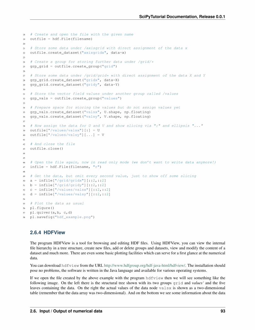
SciPyTutorial Documentation, Release 0.0.1
18 # Create and open the file with the given name19 outfile = hdf.File(filename)20
21 # Store some data under /axisgrid with direct assignment of the data x22 outfile.create_dataset("axisgridx", data=x)23
24 # Create a group for storing further data under /grid/*25 grp_grid = outfile.create_group("grid")26
27 # Store some data under /grid/grid* with direct assignment of the data X and Y28 grp_grid.create_dataset("gridx", data=X)29 grp_grid.create_dataset("gridy", data=Y)30
31 # Store the vector field values under another group called /values32 grp_vals = outfile.create_group("values")33
34 # Prepare space for storing the values but do not assign values yet35 grp_vals.create_dataset("valsx", U.shape, np.floating)36 grp_vals.create_dataset("valsy", V.shape, np.floating)37
38 # Now assign the data for U and V and show slicing via ":" and ellipsis "..."39 outfile["/values/valsx"][:] = U40 outfile["/values/valsy"][...] = V41
42 # And close the file43 outfile.close()44
45
46 # Open the file again, now in read only mode (we don’t want to write data anymore!)47 infile = hdf.File(filename, "r")48
49 # Get the data, but omit every second value, just to show off some slicing50 a = infile["/grid/gridx"][::2,::2]51 b = infile["/grid/gridy"][::2,::2]52 c = infile["/values/valsx"][::2,::2]53 d = infile["/values/valsy"][::2,::2]54
55 # Plot the data as usual56 pl.figure()57 pl.quiver(a,b, c,d)58 pl.savefig("hdf_example.png")
2.6.4 HDFView
The program HDFView is a tool for browsing and editing HDF files. Using HDFView, you can view the internalfile hierarchy in a tree structure, create new files, add or delete groups and datasets, view and modify the content of adataset and much more. There are even some basic plotting facilities which can serve for a first glance at the numericaldata.
You can download hdfview from the URL http://www.hdfgroup.org/hdf-java-html/hdfview/. The installation shouldpose no problems, the software is written in the Java language and available for various operating systems.
If we open the file created by the above example with the program hdfview then we will see something like thefollowing image. On the left there is the structural tree shown with its two groups grid and values‘ and the fiveleaves containing the data. On the right the actual values of the data node valsx is shown as a two-dimensionaltable (remember that the data array was two-dimensional). And on the bottom we see some information about the data
2.6. Input / Output of numerical data 93
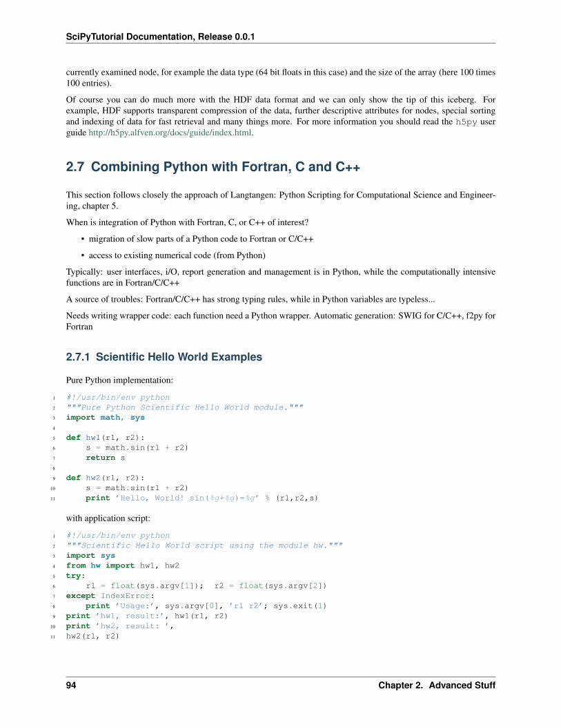
SciPyTutorial Documentation, Release 0.0.1
currently examined node, for example the data type (64 bit floats in this case) and the size of the array (here 100 times100 entries).
Of course you can do much more with the HDF data format and we can only show the tip of this iceberg. Forexample, HDF supports transparent compression of the data, further descriptive attributes for nodes, special sortingand indexing of data for fast retrieval and many things more. For more information you should read the h5py userguide http://h5py.alfven.org/docs/guide/index.html.
2.7 Combining Python with Fortran, C and C++
This section follows closely the approach of Langtangen: Python Scripting for Computational Science and Engineer-ing, chapter 5.
When is integration of Python with Fortran, C, or C++ of interest?
• migration of slow parts of a Python code to Fortran or C/C++
• access to existing numerical code (from Python)
Typically: user interfaces, i/O, report generation and management is in Python, while the computationally intensivefunctions are in Fortran/C/C++
A source of troubles: Fortran/C/C++ has strong typing rules, while in Python variables are typeless...
Needs writing wrapper code: each function need a Python wrapper. Automatic generation: SWIG for C/C++, f2py forFortran
2.7.1 Scientific Hello World Examples
Pure Python implementation:
1 #!/usr/bin/env python2 """Pure Python Scientific Hello World module."""3 import math, sys4
5 def hw1(r1, r2):6 s = math.sin(r1 + r2)7 return s8
9 def hw2(r1, r2):10 s = math.sin(r1 + r2)11 print ’Hello, World! sin(%g+%g)=%g’ % (r1,r2,s)
with application script:
1 #!/usr/bin/env python2 """Scientific Hello World script using the module hw."""3 import sys4 from hw import hw1, hw25 try:6 r1 = float(sys.argv[1]); r2 = float(sys.argv[2])7 except IndexError:8 print ’Usage:’, sys.argv[0], ’r1 r2’; sys.exit(1)9 print ’hw1, result:’, hw1(r1, r2)
10 print ’hw2, result: ’,11 hw2(r1, r2)
94 Chapter 2. Advanced Stuff
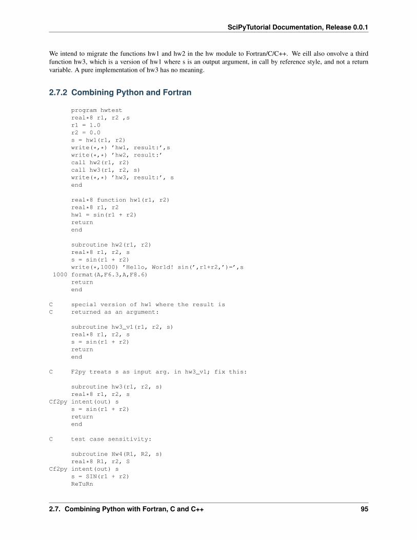
SciPyTutorial Documentation, Release 0.0.1
We intend to migrate the functions hw1 and hw2 in the hw module to Fortran/C/C++. We eill also onvolve a thirdfunction hw3, which is a version of hw1 where s is an output argument, in call by reference style, and not a returnvariable. A pure implementation of hw3 has no meaning.
2.7.2 Combining Python and Fortran
program hwtestreal*8 r1, r2 ,sr1 = 1.0r2 = 0.0s = hw1(r1, r2)write(*,*) ’hw1, result:’,swrite(*,*) ’hw2, result:’call hw2(r1, r2)call hw3(r1, r2, s)write(*,*) ’hw3, result:’, send
real*8 function hw1(r1, r2)real*8 r1, r2hw1 = sin(r1 + r2)returnend
subroutine hw2(r1, r2)real*8 r1, r2, ss = sin(r1 + r2)write(*,1000) ’Hello, World! sin(’,r1+r2,’)=’,s
1000 format(A,F6.3,A,F8.6)returnend
C special version of hw1 where the result isC returned as an argument:
subroutine hw3_v1(r1, r2, s)real*8 r1, r2, ss = sin(r1 + r2)returnend
C F2py treats s as input arg. in hw3_v1; fix this:
subroutine hw3(r1, r2, s)real*8 r1, r2, s
Cf2py intent(out) ss = sin(r1 + r2)returnend
C test case sensitivity:
subroutine Hw4(R1, R2, s)real*8 R1, r2, S
Cf2py intent(out) ss = SIN(r1 + r2)ReTuRn
2.7. Combining Python with Fortran, C and C++ 95
SciPyTutorial Documentation, Release 0.0.1
end
C end of F77 file
f2py comes automaticaly with numpy; we make a subdirectory f2py-hw and run f2py in this subdirectory:
f2py -m hw -c ../hw.f
The reuslt is the module hw.so which may be loaded into Python by an ordinary import statement.
• -m option specifies the name of the extension module
• -c indicates that f2py should compile and link the module
• –fcompiler=gfortran specifies the compiler to use (less error messages)
• f2py -c –help-fcompiler to see a list of Fortran compilers installed
• f2py -c –help-compiler to see a list of C compilers installed
Test if everything went fine:
python -c ’import hw’
We can test now the new module with the previous hwa.py program, who does not know if the module hw is writtenin Python or Fortran.
When dealing with more complicated libraries, one may want to create Python interfaces to only some of the functions,e.g.:
f2py -m hw -c --fcompiler=gfortran ../hw.f only: hw1 hw2 :
-h hw.pyf –overwrite-signature options makes f2py to write the module interfaces to a file hw.pyf that you can adjustto your needs:
f2py -m hw -h hw.pyf --overwrite-signature ../hw.ff2py -m hw -h hw.pyf --overwrite-signature ../hw.f only: hw1 hw2 :
The function hw3_v1 enables us to see one difficulty of mixing Fortran and Python. The rsult of the computations isstored in the output variable s. Since Fortran employs the call by reference for all the arguments, any change to anargument is visible in the calling code. Let us see how the interface looks like:
Bei dfault, f2py treates r1, r2, and s as input argumnets; calling hw3_v1 shows that the value of the Fortran s variableis not returned to the Python s variable in the call. The remdey is to tell f2py that s is an output parameter. We do thisby replacing in the hw.pyf file
real*8 :: s
with:
real*8 intent(out) :: s
as in subroutine hw3. The directives intent(in) and intent(out) specify input or output variables, while intent(in,out)are employed for variables for both input and output.
Compiling and linking the hw module with th emodified interface specification in hw.pyf are now performed by:
f2py -c --fcompiler=gfortran hw.pyf ../hw.f
Note thet f2py changes the interface to become more Pythonic, i.e. we write in Python:
s = hw3(r1,r2)
96 Chapter 2. Advanced Stuff
SciPyTutorial Documentation, Release 0.0.1
For a Fortran routine:
subroutine somef(in1, in2, o1, o2, o3, o4, io1)
where in1, in2 are input variables, o1, o2, o3, o4 are output variables and io1 is an input/output variable, the generatedPython interface will have i1, i2, io1 as input arguments and o1, o2, o3, o4, io1 is returend as a tuple:
o1, o2, o3, o4, io1 = somef(i1, i2, io1)
As an alternative to the modification of the .pyf file, we may insert an intent specification as a special Cf2py commentin the Fortran source code file. The safest way of writing hw3 is to specify the input/output nature of all the functionarguments:
subroutine hw3(r1,r2,s)real*8 :: r1, r2, s
Cf2py intent(in) r1Cf2py intent(in) r2Cf2py intent(out) s
s = sin(r1 + r2)returnend
2.7.3 Building an Extension Module with Distutils
The standard way for buiilding and installing Python modules uses Python’s Distutils tool which comes with thestandard Python distribution. An enhanced version of Distutils with better support for Fortran code comes with numpy.We have to create a script setup.py which calls a function steup in Distutils. Then, in order to build the extensionmodule:
python setup.py build
or to build and install:
python steup.py install
To build in the current working directory:
python setup.py build build_ext --inplace
An example of steup.py file
1 from numpy.distutils.core import Extension, setup2
3 setup(name=’hw’,4 ext_modules=[Extension(name=’hw’, sources=[’../hw.f’])],5 )
This document as pdf
2.7. Combining Python with Fortran, C and C++ 97

SciPyTutorial Documentation, Release 0.0.1
98 Chapter 2. Advanced Stuff
CHAPTER
THREE
INDICES AND TABLES
• genindex
• modindex
• search
• fenics
99

SciPyTutorial Documentation, Release 0.0.1
100 Chapter 3. Indices and tables
INDEX
Ddocstrings, 27documentation strings, 27
Ffor
statement, 25
Mmethod
object, 32
Oobject
method, 32
Sstatement
for, 25strings, documentation, 27
101