Embed Size (px)
Citation preview
Search and Ranking in Semantically Rich
Applications
Julia Stoyanovich
Submitted in partial fulfillment of the
requirements for the degree
of Doctor of Philosophy
in the Graduate School of Arts and Sciences
COLUMBIA UNIVERSITY
2010

c©2009
Julia Stoyanovich
All Rights Reserved
ABSTRACT
Search and Ranking in Semantically Rich
Applications
Julia Stoyanovich
This thesis proposes novel search and ranking approaches for semantically rich application
domains.
The central role of Data Management in today’s society may be compared to the role of
Physics in early 20th Century when it entered its Golden Age. Data is the raw matter of the
Universe of Information, and, in a process analogous to nuclear fusion, data is transformed
progressively into information, and then into knowledge.
The advent of the World Wide Web as an information exchange platform and a social
medium, both on an unprecedented scale, raises the user’s expectations with respect to
the availability and ease of access to relevant information. Web users build persistent on-
line personas: they provide information about themselves in stored profiles, register their
relationships with other users, and express their preferences with respect to information
and products. As a result, rich semantic information about the user is readily available,
or can be derived, and can be used to improve the user’s online experience, making him
more productive, more creative, and better entertained online. There is thus a need for
context-aware data management mechanisms that support a user-centric data exploration
experience, and do so efficiently on the large scale.
In a complementary trend, scientific domains, most notably the domain of life sciences,
are experiencing unprecedented growth. The ever-increasing amount of data and knowledge
requires the development of new semantically rich data management techniques that facili-
tate system-wide analysis and scientific collaboration. Literature search is a central task in
scientific research. Controlled vocabularies and ontologies that exist in this domain present
an opportunity for improving the quality of ranking.
The Web is a multifaceted medium that gives users access to a wide variety of datasets,
and satisfies diverse information needs. Some Web users look for answers to specific ques-
tions, while others browse content and explore the richness of possibilities. The notion of
relevance is intrinsically linked with preference and choice. Individual items and item col-
lections are characterized in part by the semantic relationships that hold among values of
their attributes. Exposing these semantic relationships helps the user gain a better under-
standing of the dataset, allowing him to make informed choices. This process is commonly
known as data exploration, and has applications that range from analyzing the performance
of the stock market, to identifying genetic disease susceptibility, to looking for a date.
In this thesis we propose novel search and ranking techniques that improve the user
experience and facilitate information discovery in several semantically rich application do-
mains. We show how the social context in social tagging sites can be used for user-centric
information discovery. We also propose novel ontology-aware search and ranking techniques,
and apply them to scientific literature search. Finally, we address data exploration in ranked
structured datasets, and propose a rank-aware clustering algorithm that uses semantic rela-
tionships among item attributes to facilitate information discovery.
Table of Contents
1 Introduction 1
1.1 Information Retrieval and Web Search . . . . . . . . . . . . . . . . . . . . . 3
1.1.1 Information Retrieval Models . . . . . . . . . . . . . . . . . . . . . . 4
1.1.2 Link Analysis and Authority-Based Ranking . . . . . . . . . . . . . 5
1.1.3 Evaluating the Quality of an Information Retrieval System . . . . . 7
1.1.4 Efficiency of Processing . . . . . . . . . . . . . . . . . . . . . . . . . 12
1.2 Adding a Semantic Dimension to the Web . . . . . . . . . . . . . . . . . . . 13
1.2.1 Semantic Web . . . . . . . . . . . . . . . . . . . . . . . . . . . . . . 13
1.2.2 Ontologies . . . . . . . . . . . . . . . . . . . . . . . . . . . . . . . . . 14
1.2.3 Web 2.0 . . . . . . . . . . . . . . . . . . . . . . . . . . . . . . . . . . 15
1.3 Social Web . . . . . . . . . . . . . . . . . . . . . . . . . . . . . . . . . . . . 16
1.3.1 Social Content Sites . . . . . . . . . . . . . . . . . . . . . . . . . . . 16
1.3.2 Social Information Discovery . . . . . . . . . . . . . . . . . . . . . . 17
1.4 Result Presentation for Information Discovery . . . . . . . . . . . . . . . . . 19
1.4.1 Shortcomings of Ranking . . . . . . . . . . . . . . . . . . . . . . . . 19
1.4.2 Faceted Search . . . . . . . . . . . . . . . . . . . . . . . . . . . . . . 20
1.4.3 Clustering . . . . . . . . . . . . . . . . . . . . . . . . . . . . . . . . . 20
1.5 Summary of Contributions and Thesis Outline . . . . . . . . . . . . . . . . 21
2 Search and Ranking in Collaborative Tagging Sites 25
2.1 Introduction . . . . . . . . . . . . . . . . . . . . . . . . . . . . . . . . . . . . 25
2.1.1 Search and Ranking in the Social Context . . . . . . . . . . . . . . . 25
i
2.1.2 Delicious: a Collaborative Tagging Site . . . . . . . . . . . . . . . . 26
2.1.3 Data Model . . . . . . . . . . . . . . . . . . . . . . . . . . . . . . . . 28
2.1.4 Description of the Experimental Dataset . . . . . . . . . . . . . . . . 30
2.1.5 Chapter Outline . . . . . . . . . . . . . . . . . . . . . . . . . . . . . 31
2.2 Leveraging Semantic Context to Model User Interests . . . . . . . . . . . . 31
2.2.1 Introduction . . . . . . . . . . . . . . . . . . . . . . . . . . . . . . . 31
2.2.2 Formalism . . . . . . . . . . . . . . . . . . . . . . . . . . . . . . . . . 32
2.2.3 Using Global Popularity . . . . . . . . . . . . . . . . . . . . . . . . . 33
2.2.4 Combining Global Popularity with Tags . . . . . . . . . . . . . . . . 33
2.2.5 Computing Hotlists Using the Friendship Network . . . . . . . . . . 38
2.2.6 Interest as Overlap in URLs . . . . . . . . . . . . . . . . . . . . . . . 39
2.2.7 Interest as Overlap in URLs and in Tags . . . . . . . . . . . . . . . . 40
2.2.8 Discussion . . . . . . . . . . . . . . . . . . . . . . . . . . . . . . . . . 41
2.3 Network-Aware Search . . . . . . . . . . . . . . . . . . . . . . . . . . . . . . 43
2.3.1 Introduction . . . . . . . . . . . . . . . . . . . . . . . . . . . . . . . 43
2.3.2 Formalism . . . . . . . . . . . . . . . . . . . . . . . . . . . . . . . . . 46
2.3.3 Problem Statement . . . . . . . . . . . . . . . . . . . . . . . . . . . . 47
2.4 Inverted Lists and Top-K Processing . . . . . . . . . . . . . . . . . . . . . . 47
2.4.1 Computing Exact Scores . . . . . . . . . . . . . . . . . . . . . . . . . 48
2.4.2 Top-K Processing with Exact Scores . . . . . . . . . . . . . . . . . . 48
2.4.3 Computing Score Upper-Bounds . . . . . . . . . . . . . . . . . . . . 49
2.4.4 Top-k Processing with Score Upper-Bounds . . . . . . . . . . . . . . 50
2.5 Clustering and Query Processing . . . . . . . . . . . . . . . . . . . . . . . . 53
2.5.1 Clustering Seekers . . . . . . . . . . . . . . . . . . . . . . . . . . . . 54
2.5.2 Evaluating and Tuning Clusters . . . . . . . . . . . . . . . . . . . . . 56
2.5.3 Clustering Taggers . . . . . . . . . . . . . . . . . . . . . . . . . . . . 57
2.6 Experimental Evaluation . . . . . . . . . . . . . . . . . . . . . . . . . . . . . 58
2.6.1 Implementation . . . . . . . . . . . . . . . . . . . . . . . . . . . . . . 58
2.6.2 Data and Evaluation Methods . . . . . . . . . . . . . . . . . . . . . 60
2.6.3 Performance of Global Upper-Bound . . . . . . . . . . . . . . . . . . 62
ii
2.6.4 Clustering Seekers . . . . . . . . . . . . . . . . . . . . . . . . . . . . 63
2.6.5 Effectiveness of the Clustering Quality Metric . . . . . . . . . . . . . 65
2.6.6 Clustering Taggers . . . . . . . . . . . . . . . . . . . . . . . . . . . . 67
2.7 Related Work . . . . . . . . . . . . . . . . . . . . . . . . . . . . . . . . . . . 69
2.8 Conclusion . . . . . . . . . . . . . . . . . . . . . . . . . . . . . . . . . . . . 71
3 Semantic Ranking for Life Sciences Publications 73
3.1 Introduction . . . . . . . . . . . . . . . . . . . . . . . . . . . . . . . . . . . . 73
3.1.1 Overview of MeSH . . . . . . . . . . . . . . . . . . . . . . . . . . . . 74
3.1.2 Challenges of Bibliographic Search . . . . . . . . . . . . . . . . . . . 75
3.1.3 Chapter Outline . . . . . . . . . . . . . . . . . . . . . . . . . . . . . 77
3.2 Semantics of Query Relevance . . . . . . . . . . . . . . . . . . . . . . . . . . 77
3.2.1 Motivation . . . . . . . . . . . . . . . . . . . . . . . . . . . . . . . . 77
3.2.2 Terminology . . . . . . . . . . . . . . . . . . . . . . . . . . . . . . . 78
3.2.3 Set-Based Similarity . . . . . . . . . . . . . . . . . . . . . . . . . . . 79
3.2.4 Conditional Similarity . . . . . . . . . . . . . . . . . . . . . . . . . . 80
3.2.5 Balanced Similarity . . . . . . . . . . . . . . . . . . . . . . . . . . . 80
3.3 Efficient Computation of Query Relevance . . . . . . . . . . . . . . . . . . . 81
3.3.1 Exact Computation . . . . . . . . . . . . . . . . . . . . . . . . . . . 81
3.3.2 Computation with Score Upper-Bounds . . . . . . . . . . . . . . . . 83
3.3.3 Adaptive Skyline Computation with Upper-Bounds . . . . . . . . . . 85
3.4 Experimental Evaluation . . . . . . . . . . . . . . . . . . . . . . . . . . . . . 87
3.4.1 Experimental Platform . . . . . . . . . . . . . . . . . . . . . . . . . . 87
3.4.2 Workload . . . . . . . . . . . . . . . . . . . . . . . . . . . . . . . . . 88
3.4.3 Ranked Retrieval with Score Upper-Bounds . . . . . . . . . . . . . . 89
3.4.4 Skyline Computation with Upper-Bounds . . . . . . . . . . . . . . . 92
3.5 Evaluation of Effectiveness . . . . . . . . . . . . . . . . . . . . . . . . . . . . 94
3.5.1 Baselines . . . . . . . . . . . . . . . . . . . . . . . . . . . . . . . . . 94
3.5.2 User Study . . . . . . . . . . . . . . . . . . . . . . . . . . . . . . . . 97
3.5.3 Assessment of Results . . . . . . . . . . . . . . . . . . . . . . . . . . 101
3.6 Related Work . . . . . . . . . . . . . . . . . . . . . . . . . . . . . . . . . . . 102
iii
3.7 Conclusions . . . . . . . . . . . . . . . . . . . . . . . . . . . . . . . . . . . . 104
4 Semantically Enriched Authority Propagation 107
4.1 Introduction . . . . . . . . . . . . . . . . . . . . . . . . . . . . . . . . . . . . 107
4.1.1 Semantically Enriched Ranking . . . . . . . . . . . . . . . . . . . . . 107
4.1.2 Chapter Outline . . . . . . . . . . . . . . . . . . . . . . . . . . . . . 109
4.2 Data Model . . . . . . . . . . . . . . . . . . . . . . . . . . . . . . . . . . . . 109
4.2.1 Enriched Web Graph . . . . . . . . . . . . . . . . . . . . . . . . . . . 110
4.2.2 Onto Graph . . . . . . . . . . . . . . . . . . . . . . . . . . . . . . . . 111
4.2.3 Onto Map . . . . . . . . . . . . . . . . . . . . . . . . . . . . . . . . . 111
4.2.4 Structure of the Generalized Data Graph . . . . . . . . . . . . . . . 111
4.2.5 Query Result Graph . . . . . . . . . . . . . . . . . . . . . . . . . . . 112
4.3 Authority Measures . . . . . . . . . . . . . . . . . . . . . . . . . . . . . . . 113
4.3.1 Page-Inherited Authority . . . . . . . . . . . . . . . . . . . . . . . . 113
4.3.2 Entity-Derived Authority . . . . . . . . . . . . . . . . . . . . . . . . 113
4.3.3 Untyped Authority . . . . . . . . . . . . . . . . . . . . . . . . . . . . 115
4.4 System Implementation . . . . . . . . . . . . . . . . . . . . . . . . . . . . . 115
4.4.1 Building the Generalized Data Graph . . . . . . . . . . . . . . . . . 115
4.4.2 Query Processing . . . . . . . . . . . . . . . . . . . . . . . . . . . . . 116
4.5 Experimental Evaluation . . . . . . . . . . . . . . . . . . . . . . . . . . . . . 117
4.5.1 Experimental Setup . . . . . . . . . . . . . . . . . . . . . . . . . . . 117
4.5.2 Results and Discussion . . . . . . . . . . . . . . . . . . . . . . . . . . 118
4.6 Related Work . . . . . . . . . . . . . . . . . . . . . . . . . . . . . . . . . . . 120
4.7 Conclusions . . . . . . . . . . . . . . . . . . . . . . . . . . . . . . . . . . . . 121
5 Rank-Aware Clustering of Structured Datasets 123
5.1 Introduction . . . . . . . . . . . . . . . . . . . . . . . . . . . . . . . . . . . . 123
5.1.1 Motivating User Study . . . . . . . . . . . . . . . . . . . . . . . . . . 124
5.1.2 Limitations of Clustering Algorithms . . . . . . . . . . . . . . . . . . 125
5.1.3 Challenges of Rank-Aware Clustering . . . . . . . . . . . . . . . . . 127
5.1.4 Chapter Outline . . . . . . . . . . . . . . . . . . . . . . . . . . . . . 127
iv
5.2 Formalism . . . . . . . . . . . . . . . . . . . . . . . . . . . . . . . . . . . . . 127
5.2.1 Regions and Clusters . . . . . . . . . . . . . . . . . . . . . . . . . . . 127
5.2.2 Rank-Aware Clusters . . . . . . . . . . . . . . . . . . . . . . . . . . 129
5.2.3 Problem Statement . . . . . . . . . . . . . . . . . . . . . . . . . . . . 131
5.3 Rank-Aware Subspace Clustering . . . . . . . . . . . . . . . . . . . . . . . . 131
5.3.1 Overview of Subspace Clusterings . . . . . . . . . . . . . . . . . . . 131
5.3.2 Algorithm Properties . . . . . . . . . . . . . . . . . . . . . . . . . . . 132
5.3.3 Our Approach . . . . . . . . . . . . . . . . . . . . . . . . . . . . . . 133
5.4 Experimental Evaluation of Performance . . . . . . . . . . . . . . . . . . . . 137
5.4.1 The Yahoo! Personals Dataset . . . . . . . . . . . . . . . . . . . . . 137
5.4.2 Scalability . . . . . . . . . . . . . . . . . . . . . . . . . . . . . . . . . 139
5.5 Effectiveness of Rank-Aware Clustering: A Qualitative Analysis . . . . . . . 144
5.5.1 Clustering Quality . . . . . . . . . . . . . . . . . . . . . . . . . . . . 144
5.5.2 Choosing a Clustering Quality Metric . . . . . . . . . . . . . . . . . 145
5.6 Related Work . . . . . . . . . . . . . . . . . . . . . . . . . . . . . . . . . . . 147
5.7 Conclusion . . . . . . . . . . . . . . . . . . . . . . . . . . . . . . . . . . . . 149
6 Other Contributions 151
6.1 Data Modeling in Complex Domains . . . . . . . . . . . . . . . . . . . . . . 151
6.1.1 Schema Polynomials and Applications . . . . . . . . . . . . . . . . . 151
6.1.2 Symmetric Relationships and Cardinality-Bounded Multisets . . . . 154
6.1.3 A Faceted Query Engine Applied to Archaeology . . . . . . . . . . . 156
6.2 ReoptSMART: a Learning Query Plan Cache . . . . . . . . . . . . . . . . . 157
6.2.1 Introduction . . . . . . . . . . . . . . . . . . . . . . . . . . . . . . . 157
6.2.2 AdaBoost . . . . . . . . . . . . . . . . . . . . . . . . . . . . . . . . . 159
6.2.3 Random Decision Trees . . . . . . . . . . . . . . . . . . . . . . . . . 161
6.2.4 Results . . . . . . . . . . . . . . . . . . . . . . . . . . . . . . . . . . 161
6.3 Estimating Individual Disease Susceptibility Based on Genome-Wide SNP
Arrays . . . . . . . . . . . . . . . . . . . . . . . . . . . . . . . . . . . . . . . 161
6.3.1 Introduction . . . . . . . . . . . . . . . . . . . . . . . . . . . . . . . 162
6.3.2 Methods . . . . . . . . . . . . . . . . . . . . . . . . . . . . . . . . . . 163
v
6.3.3 Results . . . . . . . . . . . . . . . . . . . . . . . . . . . . . . . . . . 164
6.3.4 Discussion . . . . . . . . . . . . . . . . . . . . . . . . . . . . . . . . . 166
7 Conclusion 167
7.1 Summary of Contributions . . . . . . . . . . . . . . . . . . . . . . . . . . . . 167
7.2 Future Research Directions . . . . . . . . . . . . . . . . . . . . . . . . . . . 168
7.2.1 Combining Different Types of Semantic Context . . . . . . . . . . . 168
7.2.2 Semantics of Provenance . . . . . . . . . . . . . . . . . . . . . . . . . 170
Bibliography 170
vi
List of Figures
2.1 Popular bookmarks in Delicious. . . . . . . . . . . . . . . . . . . . . . . . . 27
2.2 The Delicious tag cloud. . . . . . . . . . . . . . . . . . . . . . . . . . . . . . 28
2.3 Browsing bookmarks of a network member. . . . . . . . . . . . . . . . . . . 29
2.4 Hypothetical top-10 hotlists. . . . . . . . . . . . . . . . . . . . . . . . . . . 34
2.5 URLs tagged by four hypothetical Delicious users. . . . . . . . . . . . . . . 35
2.6 Seekers, networks and tagging actions. . . . . . . . . . . . . . . . . . . . . . 46
2.7 Inverted lists for Global Upper-Bound and Exact, for the tag music. . . . . 48
2.8 An example of Cluster-Seekers. . . . . . . . . . . . . . . . . . . . . . . . . 54
2.9 Performance of gNRA and gTA as k varies. . . . . . . . . . . . . . . . . . . . 61
2.10 Space overhead of Cluster-Seekers. . . . . . . . . . . . . . . . . . . . . . . 63
2.11 Correlation between NDCG and sequential accesses for Seekers-25. . . . . . 65
2.12 Space overhead of Cluster-Taggers. . . . . . . . . . . . . . . . . . . . . . . 68
3.1 A portion of the MeSH polyhierarchy. . . . . . . . . . . . . . . . . . . . . . 74
3.2 A sample scoped polyhierarchy. . . . . . . . . . . . . . . . . . . . . . . . . . 78
3.3 Two-dimensional skyline representation of results for the query G-Protein-
Coupled receptors. . . . . . . . . . . . . . . . . . . . . . . . . . . . . . . . . 86
3.4 System architecture. . . . . . . . . . . . . . . . . . . . . . . . . . . . . . . . 88
3.5 Total runtime of ranked retrieval. . . . . . . . . . . . . . . . . . . . . . . . . 91
3.6 Term similarity: percent improvement in runtime of top-k when score upper-
bounds are used. . . . . . . . . . . . . . . . . . . . . . . . . . . . . . . . . . 92
3.7 Conditional similarity: percent improvement in runtime of top-k when score
upper-bounds are used. . . . . . . . . . . . . . . . . . . . . . . . . . . . . . 93
vii
3.8 Balanced similarity: percent improvement in runtime of top-k when score
upper-bounds are used. . . . . . . . . . . . . . . . . . . . . . . . . . . . . . 94
3.9 Run-time performance of skyline computation for term similarity. . . . . . 95
3.10 Run-time performance of skyline computation for conditional similarity. . . 96
3.11 Run-time performance of skyline computation for balanced similarity. . . . 97
3.12 User study interface. . . . . . . . . . . . . . . . . . . . . . . . . . . . . . . . 99
4.1 Example of a Generalized Data Graph. . . . . . . . . . . . . . . . . . . . . . 110
5.1 Performance of BARAC as percentage of cases that completed under a
certain time limit. . . . . . . . . . . . . . . . . . . . . . . . . . . . . . . . . 140
5.2 Execution time of BuildGrid as a function of dataset size. . . . . . . . . . 141
5.3 Execution time of Join as a function of clustering dimensionality. . . . . . . 142
5.4 Execution time of Join as a function of θdom. . . . . . . . . . . . . . . . . . 142
5.5 Execution time of Join as a function of θQ. . . . . . . . . . . . . . . . . . . 143
5.6 Percentage of users for whom BARAC identified clusters, as a function of θQ.143
5.7 Top-100 scores for attribute-rank and geo-rank for user1. . . . . . . . . . . . 146
5.8 Top-100 scores for geo-rank for three users. . . . . . . . . . . . . . . . . . . 146
6.1 A screenshot of the Faceted Query Engine. . . . . . . . . . . . . . . . . . . . 157
6.2 The query template for TPCW-1. . . . . . . . . . . . . . . . . . . . . . . . . 159
6.3 Optimal plan space for query TPCW-1. . . . . . . . . . . . . . . . . . . . . 160
6.4 AdaBoost decision boundary for TPCW-1. . . . . . . . . . . . . . . . . . . . 162
6.5 RDT decision boundary for TPCW-1. . . . . . . . . . . . . . . . . . . . . . 162
6.6 Results of MutaGeneSys in scope of the HapMap genome browser. . . . . . 165
viii
List of Tables
2.1 Effect of the number of dominant tags on the performance of dominant tags. 36
2.2 Effect of interest on the performance of dominant tags. . . . . . . . . . . . 37
2.3 Effect of the agreement threshold on the effectiveness of url interest. . . 39
2.4 Relative performance of dominant tags, tag url interest, and url interest. 41
2.5 Characteristics of Network for four tags. . . . . . . . . . . . . . . . . . . . . 61
2.6 Performance of gNRA for Global Upper-Bound and Exact. . . . . . . . . . . 62
2.7 Performance of gNRA for Cluster-Seekers with 200 clusters. . . . . . . . . 64
2.8 Performance of gTA for Cluster-Seekers with 200 clusters. . . . . . . . . . 64
2.9 Using NDCG to predict performance of Cluster-Seekers for Seekers-25. . 66
2.10 Percent-improvement of Cluster-Seekers and Cluster-Taggers, compared
to Global Upper-Bound. . . . . . . . . . . . . . . . . . . . . . . . . . . . . . 66
2.11 Using NDCG to predict performance for Seekers-50. . . . . . . . . . . . . . 67
2.12 Using NDCG to predict performance for Seekers-100. . . . . . . . . . . . . . 67
3.1 Characteristics of the query workload. . . . . . . . . . . . . . . . . . . . . . 89
3.2 Ranked retrieval: processing times of Term similarity for 150 queries. . . . 89
3.3 Ranked retrieval: processing times of Conditional similarity for 150 queries. 90
3.4 Ranked retrieval: processing times of Balanced similarity for 150 queries. . . 90
3.5 Skyline computation: processing times for TermSim for 150 queries. . . . . . 95
3.6 Skyline computation: processing times for CondSim for 150 queries. . . . . . 96
3.7 Skyline computation: processing times for BalancedSim for 150 queries. . . 97
3.8 Agreement between similarity measures and user judgments. . . . . . . . . . 100
ix
3.9 Term similarity, Conditional similarity and Balanced similarity compared to
baselines. . . . . . . . . . . . . . . . . . . . . . . . . . . . . . . . . . . . . . 101
4.1 Ranking on entities. . . . . . . . . . . . . . . . . . . . . . . . . . . . . . . . 119
4.2 Ranking on pages. . . . . . . . . . . . . . . . . . . . . . . . . . . . . . . . . 119
5.1 A fictional real estate database. . . . . . . . . . . . . . . . . . . . . . . . . . 126
5.2 Structured attributes in the dating dataset. . . . . . . . . . . . . . . . . . . 138
5.3 Median, average, max and min processing times for QtopN for 100 users, with
θdom = θQ = 0.5. . . . . . . . . . . . . . . . . . . . . . . . . . . . . . . . . . 139
5.4 Characteristics of some groups identified by QtopN and QSCORE&RANK . . . 147
x
Acknowledgments
I would like to thank my adviser Professor Kenneth A. Ross for giving me the oppor-
tunity to work with him. I admire Ken’s intellect, creativity, and mental discipline. Ken
taught me how to choose research problems, and allowed me to follow my interests even
when they lay outside of his comfort zone. I am extremely grateful for Ken’s time, patience,
and for his respectful but firm guidance.
My sincere thanks go to Doctor Sihem Amer-Yahia, a friend and excellent collaborator.
Sihem instilled in me much-needed confidence, and was always very supportive, both in-
tellectually and personally. I have profound respect for Sihem’s broad perspective on data
management that is deeply rooted in real-world applications.
I am grateful to Professor Luis Gravano, with whom I have had the pleasure of inter-
acting during research group meetings and many informal discussions. I am fortunate to
know Luis as an excellent teacher; I benefited from his unique academic perspective first as
a student, and later as his teaching assistant.
I would also like to thank Professor Mihalis Yannakakis and Doctor Divesh Srivastava
who served on my thesis committee. I am grateful to Mihalis and Divesh for their time and
valuable comments.
I had an opportunity to work with many excellent researchers who inspired me both
personally and professionally. In particular, I would like to thank Professor Gerhard Weikum
who was my mentor during a summer internship at Max Planck Institute for Informatics,
and Professor Volker Markl, Doctor Guy Lohman, and Doctor Jun Rao, who were my
mentors during my summer internship at IBM Almaden.
Many others deserve my thanks for encouraging me and for supporting my intellectual
curiosity. I thank Professor Joseph E. Beck, who introduced me to Computer Science
research when I was an Undergraduate and he a Doctoral student at the University of
xi

Massachusetts, Amherst. Joe was my first academic mentor, and I am extremely grateful
for his guidance. I was also fortunate to have interacted with UMass Amherst Professors
Arnold L. Rosenberg and Robert N. Moll, and I thank them for their time and support.
I am grateful to my teachers and classmates at the Belgrade Mathematical High School,
and to the school’s Principal Doctor Milan Raspopovic, who created an exceptional, intel-
lectually rigorous environment at the school.
On a more personal note, this dissertation would not have been possible without help
and support from my family and friends. I am deeply grateful to my parents, Ljudmila
and Dragan Stojanovic, for their unconditional love and continuous encouragement. My
mother has always been my greatest inspiration; she is the first Doctor Stojanovic in our
family, and I am merely following in her footsteps. I thank my husband, Oleg Sarkissov,
for patiently helping me through nervous breakdowns and for sharing the happy moments.
Finally, I would like to acknowledge the financial support of the National Science Foun-
dation (grant IIS-0121239) and of the National Institute of Health (grant 5 U54 CA121852-
05).
Each chapter gratefully acknowledges the co-authors of the work on which the chapter
is based. I will be referring to myself and my respective co-authors using the pronoun we
in the remainder of this thesis.
xii

In loving memory of my grandfather Zyama Avramovich Lurie.
xiii

xiv
CHAPTER 1. INTRODUCTION 1
Chapter 1
Introduction
The central role of Data Management in today’s society may be compared to the role of
Physics in early 20th Century when it entered its Golden Age. Data is the raw matter of the
Universe of Information, and, in a process analogous to nuclear fusion, data is transformed
progressively into information, and then into knowledge.
Information is, in fact, so important, that even philosophers are starting to get inter-
ested. An emerging discipline of Philosophy of Information [Floridi, 2009b] postulates that
“to be is to be an informational entity” [Ess, 2009]. According to this new doctrine, history
is synonymous with the information age, since prehistory is the age in human development
that precedes the availability of recording systems.
The information-based nature of our society has only recently become apparent, and
is clearly linked to the wide-spread adoption of the World Wide Web as a platform for
information dissemination and sharing. Nowadays the most advanced economies highly
depend on information technologies in their functioning and growth. It has been argued that
the world’s seven larges economies, formerly known as G7, qualify as information societies,
because at least 70% of their gross domestic product depends on intangible information-
related goods, not on material goods, which are the physical output of agricultural or
manufacturing processes [Floridi, 2009a].
The World Wide Web is, without a doubt, one of the greatest inventions of the 20th
century. The Web is a living and breathing organism that is interesting both as a phe-
nomenon unto itself, and because of the multitude of other phenomena that it supports
and enables. The advent of the World Wide Web sparked the generation and exchange of
information on an unprecedented scale, presenting the data management community with
vital opportunities and interesting challenges.
A central data management challenge that arises in the Internet age is the transformation
of data into knowledge. A particular aspect of this challenge may be phrased as follows.
Provided that the burden of synthesizing knowledge from relevant information rests on the
user, how can the system point the user towards the information that is relevant? After all,
2 CHAPTER 1. INTRODUCTION
the complexity of finding a needle in a haystack increases with the size of the haystack.1
The young 21st century has already unveiled its first great discoveries, not last among
which is the popularization of online social networking and of social content sites. Of these
sites there is a great variety – from the versatile Facebook platform that supports many
types of content and various degrees of user involvement, to the minimalist Twitter, in
which users communicate by publishing laconic status updates, or tweets.
Social content sites are backed by the World Wide Web, and are responsible for enriching
or, as some would say, polluting the global information space by orders of magnitude more
data. These sites bring about a shift in the traditional paradigm of information dissemi-
nation, in which there are far fewer producers of information than there are consumers. In
contrast to traditional media, and to Internet-based publishing of the pre-social era, users
of social content sites are both producers and raters of information, as well as information
consumers. The blurring of the line between producers and consumers of content results in
democratization of information, providing a powerful participation incentive.
In a related trend, many scientific domains, most notably the domain of life sciences,
are experiencing unprecedented growth. The recent complete sequencing of the Human
Genome, and the tremendous advances in experimental technology, are rapidly bringing
about new scientific knowledge. The ever-increasing amount of data and knowledge in
life sciences in turn requires the development of new semantically rich data management
techniques that facilitate scientific research and collaboration.
An important challenge posed by the data management needs of the scientific community
may be phrased as follows. Provided that high-quality knowledge bases are available that
summarize the state of the art in a scientific field, how can the system use this knowledge
to identify relevant information, enabling further scientific advances?
The Web is a multifaceted medium that gives users access to a wide variety of datasets,
and satisfies diverse information needs. Some Web users look for answers to specific ques-
tions, while others browse content and explore the richness of possibilities. The notion of
relevance is intrinsically linked with preference and choice. Preferences are known to change
based on temporal aspects, one of which is the change in availability of items (be it physical
products of information entities), or in a user’s belief about the availability of items [Hansson
and Grune-Yanoff, 2006]. The process by which a user ascertains the availability of items
is known as data exploration.
Individual items and item collections are characterized in part by the semantic rela-
tionships that hold among values of their attributes. These relationships may be known
a priori, e.g., all 10-story buildings in the US have an elevator. Alternatively, these rela-
tionships may need to be derived, using inference or statistical tools. Exposing semantic
relationships that hold among item attributes helps the user gain a better understanding
1Proof is left as an exercise for the reader.
CHAPTER 1. INTRODUCTION 3
of the dataset, allowing him to make informed choices. Data exploration is a common task,
with application ranging from analyzing the performance of the stock market, to identifying
genetic disease susceptibility, to looking for a date.
Success of data exploration depends critically on the availability of effective analysis
and presentation methods. An important data management question is then: Provided
that a user’s preferences depend in part on the semantic relationships that hold among item
attributes, how can the system effectively derive these relationships and present them to the
user, facilitating data exploration?
This thesis proposes novel search and ranking methods aimed at improving the user
experience and facilitating information discovery in semantically rich applications. In the
remainder of this section, we give an overview of the state of the art in related data man-
agement areas, and outline our contributions.
1.1 Information Retrieval and Web Search
In Information Retrieval (IR), a user expresses his information need with a query q. An IR
system evaluates the query against a document corpus D, and identifies a set of answers
A ⊆ D that are conjectured by the system to satisfy the user’s information need. The
documents in A are said to match the query q. The language used to express the query,
and the mechanism by which answers are identified, depend on the retrieval model used by
the IR system. We will describe several common retrieval models in Section 1.1.1.
In IR, documents are typically drawn from a large corpus, and relevant documents are
identified. In real-world IR scenarios such as Web search, or scientific literature search,
many more relevant documents are typically identified than any one user is willing to read.
Further, not all documents that are identified as answers carry equal relevance to the user’s
query. Therefore, the system must choose a portion of the result set to present to the user,
motivating the need for ranking. Results are commonly returned in the form of a ranked
list, with the goal of presenting to the user documents that are conjectured by the system
to have high relevance to the user’s query. To this end, IR systems define a ranking function
R : D → R that, for a fixed query, associates each document d ∈ D with a real number. R
defines a natural ordering on the documents in the collection, and expresses the extent to
which each document matches the query.
Information Retrieval methods were originally developed for searching document col-
lections to which we currently refer as Digital Libraries, such as the on-line version of the
Library of Congress (www.loc.gov) or the PubMed Central repository of scientific articles
(www.pubmedcentral.nih.gov). These collections are curated and generally contain docu-
ments of high quality, in the sense that a document that covers a particular topic is usually
authored by an expert on that topic. Further, the vocabulary used in a document is usu-
ally representative of the document’s semantic content. This is to be contrasted with the
4 CHAPTER 1. INTRODUCTION
document corpus that is the World Wide Web, in which there is a high degree of variability
with respect to the quality of information. Authors of Web content have a varying degree
of expertise on the subjects they cover. Additionally, the words used on a particular web
page may not truthfully reflect the semantic content of the page, a phenomenon known as
search engine spamming. Based on these considerations, new IR methods were developed
that incorporate both a document’s textual relatedness to a user’s query, and a document’s
authority. We will give an overview of these methods in Section 1.1.2.
An important and difficult question is how to properly evaluate the performance of an
IR system. We discuss some approaches for evaluating the quality of retrieval and ranking
in Section 1.1.3, and give an overview of performance-related issues in Section 1.1.4.
1.1.1 Information Retrieval Models
The IR models of this section represent queries and documents in a corpus as collections,
such as sets or vectors, of index terms. Index terms t1, t2, . . . tn are elements of a vocabulary
T that typically corresponds to words in the natural language of the collection.
The Boolean model is based on set theory and Boolean algebra. In this model queries
are specified as conjunctions (keyword AND), disjunctions (keyword OR), or negations
(keyword NOT) of index terms. A query is an arbitrary Boolean expression over the terms
from T , which is converted by the system to disjunctive normal form. Each document
d ∈ D is in turn represented as a conjunction of the terms that occur in the document.
Suppose that a vocabulary is given that consists of three terms; we represent the vo-
cabulary as a set T = {t1, t2, t3}2. Suppose also that a query is given by the Boolean
expression q = t1 ∧ (t2 ∨ ¬t3). This query can be equivalently re-written in disjunctive
normal form as qDNF = (t1∧ t2∧ t3)∨ (t1∧ t2∧¬t3)∨ (t1∧¬t2∧¬t3). Document di = t1∧ t2
will match the query, since it matches the second conjunctive term in qDNF . On the other
hand, document dj = t1 ∧ t3 will not match q.
For each document d ∈ D, the Boolean model will predict that the document is either
relevant to a query q or that it is irrelevant.
The vector space model, which was first introduced in [Salton et al., 1975], relaxes the
assumption that a document is either relevant or irrelevant to a query. Unlike the Boolean
model, the vector space model incorporates term weights, and supports partial matching.
In the vector space model, the vocabulary of index terms T is represented by a vector,
with length equal to the size of the vocabulary. Queries and documents are represented
by vectors of non-binary weights, with each position corresponding to a term in T . The
weights are used to compute the degree of similarity between a query and a document. So,
for a query ~q and a document ~d, we compute similarity as the cosine of the angle between
2This example is based on the example in Section 2.5.2 of [Baeza-Yates and Ribeiro-Neto, 1999].
CHAPTER 1. INTRODUCTION 5
these two vectors in the space of T :
sim(~d, ~q) =~d • ~q
|~d| × |~q|(1.1)
How well the model will match human intuition clearly depends on a meaningful choice
for the weights. A classic weighting scheme, known as tf-idf, weights a document term
according to how often the term appears in the document. This portion of the weight, called
term frequency, or tf, models the intuition that a term that is mentioned in a document more
often is more representative of the document’s content than another term that is mentioned
less often. The tf weight is normalized by the total frequency of the term in the corpus.
This normalization, referred to as inverse document frequency, or idf, penalizes terms that
frequently occur in the corpus, because such terms may be less informative.
We described two classical retrieval models in IR. Many other successful models exist and
are used today in IR systems. The probabilistic model attempts to estimate the probability
that the user will find the document d relevant to a query q, given the representations of
d and q. A family of probabilistic IR models are the language models that are based on a
probabilistic mechanism for generating text. Given a query q and a document d, the system
computes the probability that q was generated by the language model of d, and ranks the
retrieved documents on this probability [Croft and Lafferty, 2003].
The fuzzy set model assumes that each query term defines a fuzzy set, and that each
document has a degree of membership (usually less than 1) in this set. The extended Boolean
model allows for the weighting of Boolean terms. A variety of extensions, and of new models,
have been considered in the literature. However, this thesis does not use any of the later
models, and so a complete review is beyond the scope of this work. We refer the reader
to [Baeza-Yates and Ribeiro-Neto, 1999; Manning et al., 2008] for a comprehensive review
of other approaches.
Most IR models lend themselves well to ranking, because they incorporate a notion of
non-binary similarity between the query and the document. An exception is the Boolean
retrieval model, which produces binary outcomes, and as such does not naturally support
ranking. In addition to relevance, modern IR systems also incorporate a notion of authority
into the ranking, and we discuss this topic next.
1.1.2 Link Analysis and Authority-Based Ranking
The World Wide Web became a prominent medium for information discovery in the early
1990s. By that time IR was already a mature field that developed primarily based on
information discovery tasks over large curated document collections. The advent of the
Web prompted the field of IR to adapt, and to develop techniques appropriate both for
the ever-increasing size of this dynamic collection, and for the heterogeneity in information
quality.
6 CHAPTER 1. INTRODUCTION
A crucial property of the Web that motivates some of the early advances in Web-based
retrieval and ranking is that the Web has a natural graph structure. The Web is comprised
of pages with hyperlinks to other pages. For example, a Web page of a Computer Science
PhD student may contain a link pointing to her adviser’s homepage:
<a href=’’http://www.cs.columbia.edu/~kar’’>Homepage of Kenneth A. Ross</a>
A key observation made by Kleinberg in a seminal paper [Kleinberg, 1999] is that hy-
perlinks of this kind may be viewed as endorsements. A page that links to another page
implicitly endorses the target page, giving it prominence, commonly referred to as authority.
At roughly the same time Brin and Page developed the PageRank algorithm [Brin and
Page, 1998] that models the authority of a Web page based on the probability that it will
be visited by a random surfer who uses the link structure of the Web. PageRank serves as
basis for the search algorithm employed by Google, a leading Web search engine. We now
give a brief description of these two influential algorithms.
The Hyperlink-Induced Topic Search (HITS) algorithm, also known as Hubs and Au-
thorities, was proposed in [Kleinberg, 1999]. HITS uses the link structure of the web graph
to identify, in a query-specific or topic-specific manner, a set of authoritative pages, and
a set of hub pages that join the authorities into the link structure. The Web is modeled
as a directed graph G = (V,E), where nodes V correspond to pages, and a directed edge
(p, q) ∈ E indicates the presence of a link from page p to page q.
The algorithm starts by constructing a relatively small subgraph of the Web, called the
root set, that contains a high number of query-relevant pages. The root set is then expanded
to include adjacent pages – pages pointed to by the pages in the root set, and pages pointing
to the pages in the root set. The resulting sub-graph of the Web graph, referred to as Gσ,
has a high chance of containing some authorities, and these authorities are identified using
an iterative procedure.
Each web page p among the nodes of Gσ is assigned two weights – an authority weight
x〈p〉 and a hub weight y〈p〉. Both kinds of weights are initialized uniformly for all pages, and
are updated iteratively. The update procedure builds on the intuition that a page p that
points to many pages should receive a high hub weight (y), while a page that is pointed to
by many pages should receive a high authority weight (x). Given weights {x〈p〉} and {y〈p〉},
two operations are applied in turn and update the weights as follows:
x〈p〉 ← Σq:(q,p)∈Ey〈p〉 (1.2)
y〈p〉 ← Σq:(q,p)∈Ex〈p〉 (1.3)
Weights are normalized after each iterative step. Eventually, the system converges to a
solution and the iteration stops.
CHAPTER 1. INTRODUCTION 7
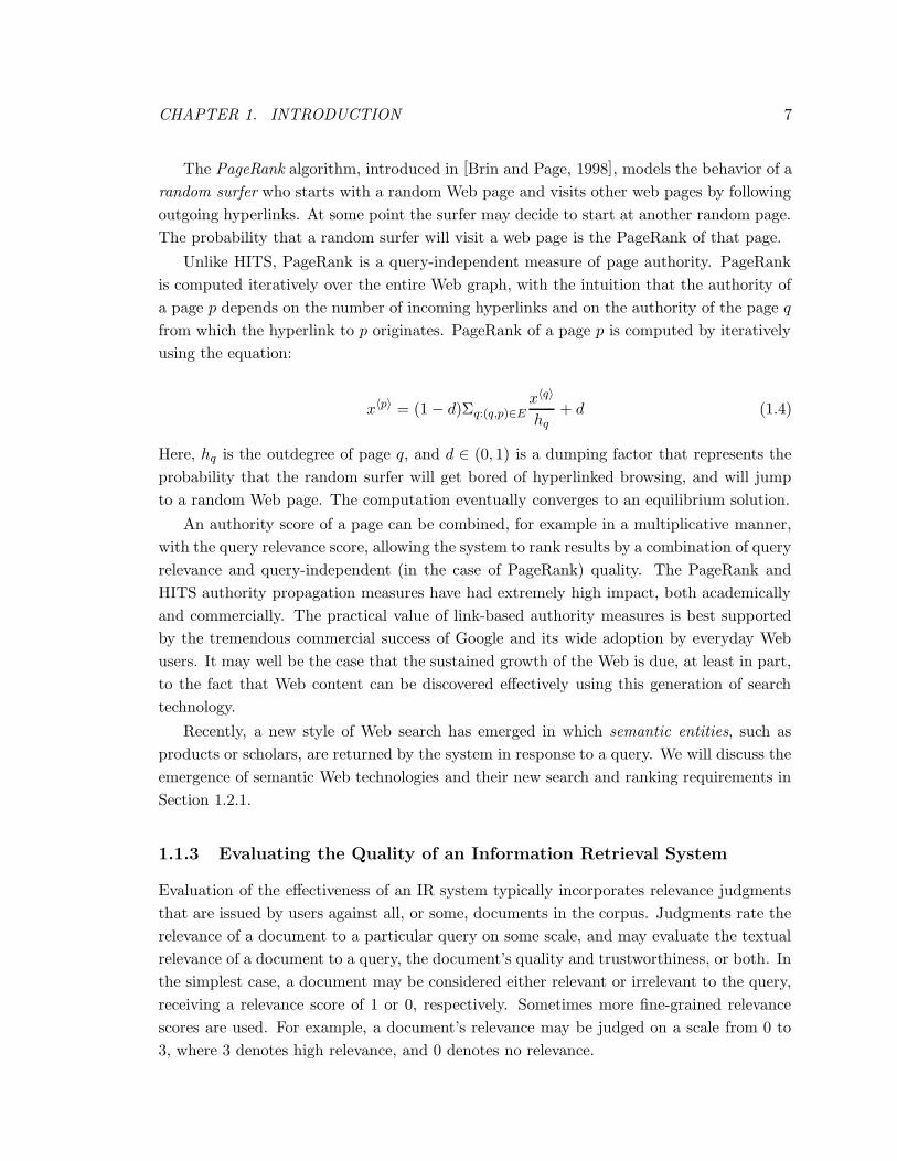
The PageRank algorithm, introduced in [Brin and Page, 1998], models the behavior of a
random surfer who starts with a random Web page and visits other web pages by following
outgoing hyperlinks. At some point the surfer may decide to start at another random page.
The probability that a random surfer will visit a web page is the PageRank of that page.
Unlike HITS, PageRank is a query-independent measure of page authority. PageRank
is computed iteratively over the entire Web graph, with the intuition that the authority of
a page p depends on the number of incoming hyperlinks and on the authority of the page q
from which the hyperlink to p originates. PageRank of a page p is computed by iteratively
using the equation:
x〈p〉 = (1− d)Σq:(q,p)∈E
x〈q〉
hq+ d (1.4)
Here, hq is the outdegree of page q, and d ∈ (0, 1) is a dumping factor that represents the
probability that the random surfer will get bored of hyperlinked browsing, and will jump
to a random Web page. The computation eventually converges to an equilibrium solution.
An authority score of a page can be combined, for example in a multiplicative manner,
with the query relevance score, allowing the system to rank results by a combination of query
relevance and query-independent (in the case of PageRank) quality. The PageRank and
HITS authority propagation measures have had extremely high impact, both academically
and commercially. The practical value of link-based authority measures is best supported
by the tremendous commercial success of Google and its wide adoption by everyday Web
users. It may well be the case that the sustained growth of the Web is due, at least in part,
to the fact that Web content can be discovered effectively using this generation of search
technology.
Recently, a new style of Web search has emerged in which semantic entities, such as
products or scholars, are returned by the system in response to a query. We will discuss the
emergence of semantic Web technologies and their new search and ranking requirements in
Section 1.2.1.
1.1.3 Evaluating the Quality of an Information Retrieval System
Evaluation of the effectiveness of an IR system typically incorporates relevance judgments
that are issued by users against all, or some, documents in the corpus. Judgments rate the
relevance of a document to a particular query on some scale, and may evaluate the textual
relevance of a document to a query, the document’s quality and trustworthiness, or both. In
the simplest case, a document may be considered either relevant or irrelevant to the query,
receiving a relevance score of 1 or 0, respectively. Sometimes more fine-grained relevance
scores are used. For example, a document’s relevance may be judged on a scale from 0 to
3, where 3 denotes high relevance, and 0 denotes no relevance.
8 CHAPTER 1. INTRODUCTION
1.1.3.1 Set-Based Measures
We now describe some typical ways that relevance judgments may be used to quantify the
performance of an IR system. These and other methods are described in detail in [Baeza-
Yates and Ribeiro-Neto, 1999]. Given a query q, and a document collection D, we may use
relevance judgments to partition the collection into two mutually exclusive sets: set R of
relevant documents, and set I of irrelevant documents. To quantify the performance of a
retrieval-only IR system (one that does not do any ranking), we may consider the set of all
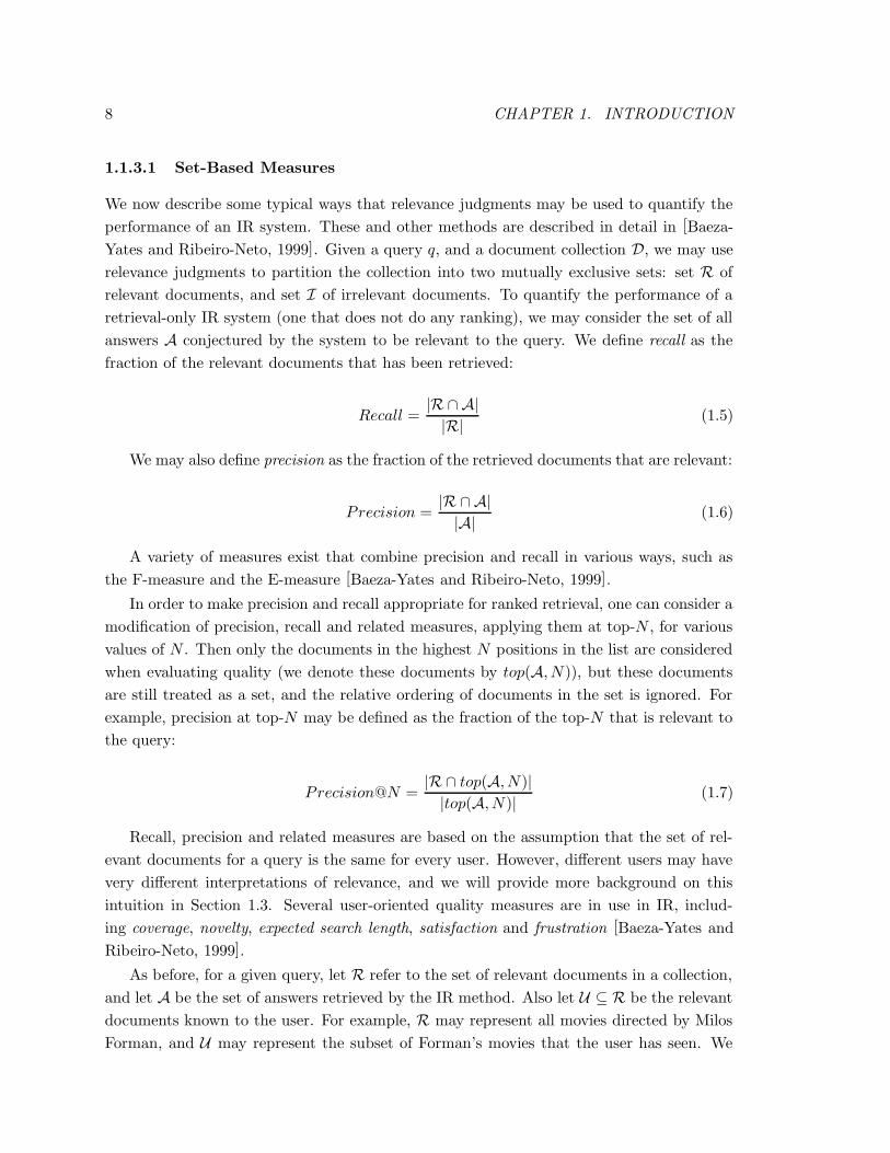
answers A conjectured by the system to be relevant to the query. We define recall as the
fraction of the relevant documents that has been retrieved:
Recall =|R ∩ A|
|R|(1.5)
We may also define precision as the fraction of the retrieved documents that are relevant:
Precision =|R ∩A|
|A|(1.6)
A variety of measures exist that combine precision and recall in various ways, such as
the F-measure and the E-measure [Baeza-Yates and Ribeiro-Neto, 1999].
In order to make precision and recall appropriate for ranked retrieval, one can consider a
modification of precision, recall and related measures, applying them at top-N , for various
values of N . Then only the documents in the highest N positions in the list are considered
when evaluating quality (we denote these documents by top(A, N)), but these documents
are still treated as a set, and the relative ordering of documents in the set is ignored. For
example, precision at top-N may be defined as the fraction of the top-N that is relevant to
the query:
Precision@N =|R ∩ top(A, N)|
|top(A, N)|(1.7)
Recall, precision and related measures are based on the assumption that the set of rel-
evant documents for a query is the same for every user. However, different users may have
very different interpretations of relevance, and we will provide more background on this
intuition in Section 1.3. Several user-oriented quality measures are in use in IR, includ-
ing coverage, novelty, expected search length, satisfaction and frustration [Baeza-Yates and
Ribeiro-Neto, 1999].
As before, for a given query, let R refer to the set of relevant documents in a collection,
and let A be the set of answers retrieved by the IR method. Also let U ⊆ R be the relevant
documents known to the user. For example, R may represent all movies directed by Milos
Forman, and U may represent the subset of Forman’s movies that the user has seen. We
CHAPTER 1. INTRODUCTION 9
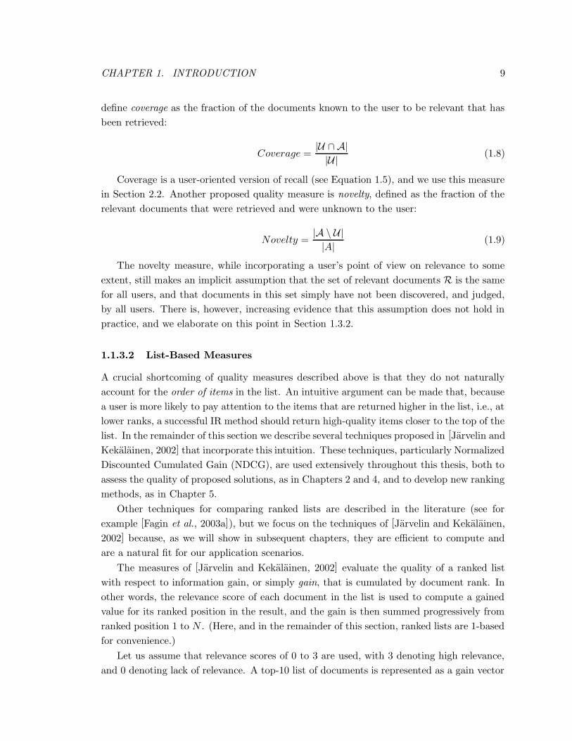
define coverage as the fraction of the documents known to the user to be relevant that has
been retrieved:
Coverage =|U ∩ A|
|U|(1.8)
Coverage is a user-oriented version of recall (see Equation 1.5), and we use this measure
in Section 2.2. Another proposed quality measure is novelty, defined as the fraction of the
relevant documents that were retrieved and were unknown to the user:
Novelty =|A \ U|
|A|(1.9)
The novelty measure, while incorporating a user’s point of view on relevance to some
extent, still makes an implicit assumption that the set of relevant documents R is the same
for all users, and that documents in this set simply have not been discovered, and judged,
by all users. There is, however, increasing evidence that this assumption does not hold in
practice, and we elaborate on this point in Section 1.3.2.
1.1.3.2 List-Based Measures
A crucial shortcoming of quality measures described above is that they do not naturally
account for the order of items in the list. An intuitive argument can be made that, because
a user is more likely to pay attention to the items that are returned higher in the list, i.e., at
lower ranks, a successful IR method should return high-quality items closer to the top of the
list. In the remainder of this section we describe several techniques proposed in [Jarvelin and
Kekalainen, 2002] that incorporate this intuition. These techniques, particularly Normalized
Discounted Cumulated Gain (NDCG), are used extensively throughout this thesis, both to
assess the quality of proposed solutions, as in Chapters 2 and 4, and to develop new ranking
methods, as in Chapter 5.
Other techniques for comparing ranked lists are described in the literature (see for
example [Fagin et al., 2003a]), but we focus on the techniques of [Jarvelin and Kekalainen,
2002] because, as we will show in subsequent chapters, they are efficient to compute and
are a natural fit for our application scenarios.
The measures of [Jarvelin and Kekalainen, 2002] evaluate the quality of a ranked list
with respect to information gain, or simply gain, that is cumulated by document rank. In
other words, the relevance score of each document in the list is used to compute a gained
value for its ranked position in the result, and the gain is then summed progressively from
ranked position 1 to N . (Here, and in the remainder of this section, ranked lists are 1-based
for convenience.)
Let us assume that relevance scores of 0 to 3 are used, with 3 denoting high relevance,
and 0 denoting lack of relevance. A top-10 list of documents is represented as a gain vector
10 CHAPTER 1. INTRODUCTION
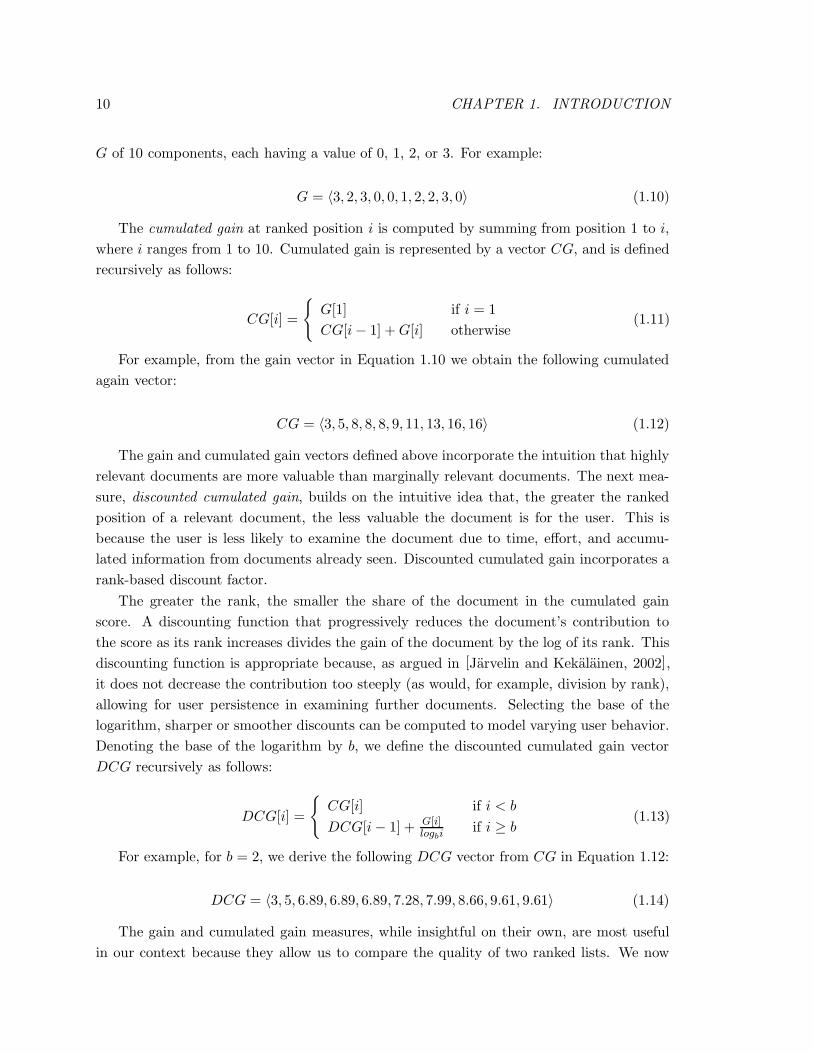
G of 10 components, each having a value of 0, 1, 2, or 3. For example:
G = 〈3, 2, 3, 0, 0, 1, 2, 2, 3, 0〉 (1.10)
The cumulated gain at ranked position i is computed by summing from position 1 to i,
where i ranges from 1 to 10. Cumulated gain is represented by a vector CG, and is defined
recursively as follows:
CG[i] =
{
G[1] if i = 1
CG[i− 1] + G[i] otherwise(1.11)
For example, from the gain vector in Equation 1.10 we obtain the following cumulated
again vector:
CG = 〈3, 5, 8, 8, 8, 9, 11, 13, 16, 16〉 (1.12)
The gain and cumulated gain vectors defined above incorporate the intuition that highly
relevant documents are more valuable than marginally relevant documents. The next mea-
sure, discounted cumulated gain, builds on the intuitive idea that, the greater the ranked
position of a relevant document, the less valuable the document is for the user. This is
because the user is less likely to examine the document due to time, effort, and accumu-
lated information from documents already seen. Discounted cumulated gain incorporates a
rank-based discount factor.
The greater the rank, the smaller the share of the document in the cumulated gain
score. A discounting function that progressively reduces the document’s contribution to
the score as its rank increases divides the gain of the document by the log of its rank. This
discounting function is appropriate because, as argued in [Jarvelin and Kekalainen, 2002],
it does not decrease the contribution too steeply (as would, for example, division by rank),
allowing for user persistence in examining further documents. Selecting the base of the
logarithm, sharper or smoother discounts can be computed to model varying user behavior.
Denoting the base of the logarithm by b, we define the discounted cumulated gain vector
DCG recursively as follows:
DCG[i] =
{
CG[i] if i < b
DCG[i− 1] + G[i]logbi
if i ≥ b(1.13)
For example, for b = 2, we derive the following DCG vector from CG in Equation 1.12:
DCG = 〈3, 5, 6.89, 6.89, 6.89, 7.28, 7.99, 8.66, 9.61, 9.61〉 (1.14)
The gain and cumulated gain measures, while insightful on their own, are most useful
in our context because they allow us to compare the quality of two ranked lists. We now
CHAPTER 1. INTRODUCTION 11
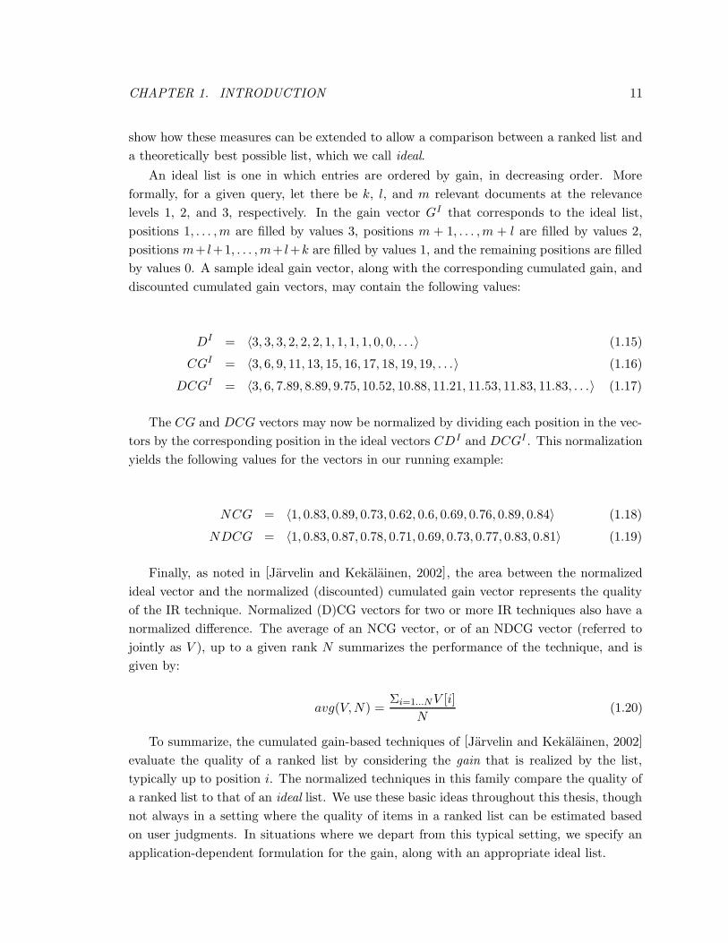
show how these measures can be extended to allow a comparison between a ranked list and
a theoretically best possible list, which we call ideal.
An ideal list is one in which entries are ordered by gain, in decreasing order. More
formally, for a given query, let there be k, l, and m relevant documents at the relevance
levels 1, 2, and 3, respectively. In the gain vector GI that corresponds to the ideal list,
positions 1, . . . ,m are filled by values 3, positions m + 1, . . . ,m + l are filled by values 2,
positions m+ l+1, . . . ,m+ l+k are filled by values 1, and the remaining positions are filled
by values 0. A sample ideal gain vector, along with the corresponding cumulated gain, and
discounted cumulated gain vectors, may contain the following values:
DI = 〈3, 3, 3, 2, 2, 2, 1, 1, 1, 1, 0, 0, . . .〉 (1.15)
CGI = 〈3, 6, 9, 11, 13, 15, 16, 17, 18, 19, 19, . . .〉 (1.16)
DCGI = 〈3, 6, 7.89, 8.89, 9.75, 10.52, 10.88, 11.21, 11.53, 11.83, 11.83, . . .〉 (1.17)
The CG and DCG vectors may now be normalized by dividing each position in the vec-
tors by the corresponding position in the ideal vectors CDI and DCGI . This normalization
yields the following values for the vectors in our running example:
NCG = 〈1, 0.83, 0.89, 0.73, 0.62, 0.6, 0.69, 0.76, 0.89, 0.84〉 (1.18)
NDCG = 〈1, 0.83, 0.87, 0.78, 0.71, 0.69, 0.73, 0.77, 0.83, 0.81〉 (1.19)
Finally, as noted in [Jarvelin and Kekalainen, 2002], the area between the normalized
ideal vector and the normalized (discounted) cumulated gain vector represents the quality
of the IR technique. Normalized (D)CG vectors for two or more IR techniques also have a
normalized difference. The average of an NCG vector, or of an NDCG vector (referred to
jointly as V ), up to a given rank N summarizes the performance of the technique, and is
given by:
avg(V,N) =Σi=1...NV [i]
N(1.20)
To summarize, the cumulated gain-based techniques of [Jarvelin and Kekalainen, 2002]
evaluate the quality of a ranked list by considering the gain that is realized by the list,
typically up to position i. The normalized techniques in this family compare the quality of
a ranked list to that of an ideal list. We use these basic ideas throughout this thesis, though
not always in a setting where the quality of items in a ranked list can be estimated based
on user judgments. In situations where we depart from this typical setting, we specify an
application-dependent formulation for the gain, along with an appropriate ideal list.
12 CHAPTER 1. INTRODUCTION
1.1.4 Efficiency of Processing
As mentioned throughout this section, both classic and Web-based Information Retrieval
methods are usually applied to very large document collections, and are expected to yield
sub-second response times in multi-user environments. Therefore IR methods must be built
with efficiency considerations in mind.
The seminal work of Brin and Page [Brin and Page, 1998] in which the PageRank algo-
rithm was first described also devotes significant attention to the scalable implementation of
the Google prototype. This early paper outlines the challenges of large scale Web crawling,
indexing, and searching, and presents the distributed file system construct fundamental to
Google’s architecture called BigFiles, a precursor of the Google File System (GFS) [Ghe-
mawat et al., 2003]. Google subsequently implemented BigTable, a proprietary database
system built on GFS that departs from the typical convention of a fixed number of columns
and is instead described by the authors as a sparse, distributed multi-dimensional sorted
map [Chang et al., 2006]. BigTable in turn supports the MapReduce framework, introduced
by Google in [Dean and Ghemawat, 2006], which enables distributed computation over large
scale datasets in a cluster environment.
The MapReduce framework supports two main operations: Map and Reduce. The Map
operation is executed by the master node, which partitions the problem into sub-problems
and assigns the sub-problems to worker nodes. The Reduce step involves combining the
answers to sub-problems, and returning the combined solution as the final answer. The
MapReduce framework is proprietary to Google.
Apache Hadoop is an open-source software framework that was inspired by MapReduce
and by the Google File System.
An inverted index, also known as an inverted file, is a conceptual data structure used
by many search algorithms in IR and Web search. An inverted index stores a mapping
from content, such as vocabulary terms or phrases, to its location in a document, allowing
full-text search. In [Zobel et al., 1998] the performance of inverted files was extensively
analyzed, demonstrating the scalability, space efficiency, and good update performance of
this data structure.
Inverted files have been used in a variety of applications including some influential
top-K processing algorithms. A seminal paper [Fagin et al., 2003c] presents the threshold
algorithm (TA), which is provably optimal in terms of run-time performance, and is used
for aggregating scores over inverted file entries. Given a query q represented by a set of
index terms, and a collection of inverted files, the TA algorithm determines the k items with
the highest over-all score. The algorithm builds on an intuition that high-scoring items will
appear closer to the top of all relevant inverted lists than would lower-scoring items.
CHAPTER 1. INTRODUCTION 13
1.2 Adding a Semantic Dimension to the Web
1.2.1 Semantic Web
Information Retrieval and Web search techniques outlined in Section 1.1 reason over queries
and documents in a corpus by considering the terms that make up these queries and docu-
ments. These techniques manipulate terms as symbols, and do not consider the semantics,
or meaning of the vocabulary.
The Semantic Web, or a Web with meaning, is an ambitious effort that aims to create
a Web-wide machine-processable representation of real-world entities and of relationships
between these entities. The World Wide Web Consortium (W3C) leads the Semantic Web
effort, and gives the following definition of the initiative 3 :
The Semantic Web provides a common framework that allows data to be shared and
reused across application, enterprise, and community boundaries.
According to the Wikipedia entry for Semantic Web (as of September 17, 2009): “At its
core, the Semantic Web comprises a set of design principles, collaborative working groups,
and a variety of enabling technologies. Some elements of the Semantic Web are expressed as
prospective future possibilities that are yet to be implemented or realized. Other elements
of the Semantic Web are expressed in formal specifications. Some of these include Resource
Description Framework (RDF), a variety of data interchange formats (e.g., RDF/XML, N3,
Turtle, N-Triples), and notations such as RDF Schema (RDFS) and the Web Ontology
Language (OWL), all of which are intended to provide a formal description of concepts,
terms, and relationships within a given knowledge domain.”
For the promise of Semantic Web to be realized on the full scale of the Web, Web data
should be published in languages specifically designed for semantic annotation such as RDF,
OWL and XML, so as to enable semantic tagging of entities. For example, a Web page that
mentions the entity Cat must use semantic mark-up that may look like4 :
<item rdf:about=http://dbpedia.org/resource/Cat>Cat</item>
Semantic annotations of this kind refer to entries in an ontology, a formal representation
of a set of concepts that defines the domain for each concept, and specifies the relationship
between concepts. Ontologies provide a machine-processable representation, and support
reasoning and inference.
While the goal of semantically annotating the whole Web remains elusive, due mostly
to the high cost of adoption of a common representation framework, and to the difficulty
(or perhaps impossibility) of schema design and maintenance at Web scale, Semantic Web
technologies have been successfully used in certain domains. We describe some challenges
3Definition from www.w3.org/2001/sw, downloaded on September 17, 2009.
4This example is from en.wikipedia.org/wiki/Semantic_Web, downloaded on September 17, 2009.
14 CHAPTER 1. INTRODUCTION
related to the creation and maintenance of ontologies, and give examples of success stories,
in the following section.
1.2.2 Ontologies
The building and maintenance of an ontology is a top-down process that requires an exten-
sive amount of curation. Consider for example the process of creating and maintaining an
ontology in the domain of life sciences. An ontology represents a consensus among domain
experts regarding the state of knowledge in a particular field. This consensus is particularly
difficult to achieve in dynamic fields where knowledge constantly evolves. At the same time,
ontologies are most valuable in such fields, because they do not simply record the state of
the art for posterity, but rather are aimed at supporting community-wide collaboration and
the advancement of science.
In order to create an ontology, domain experts must first agree on the vocabulary.
If an ontology represents a consensus view of several sub-fields within a field (e.g., an
ontology of gene products across species), reaching an agreement with respect to a common
vocabulary may be even more difficult. Having agreed on a vocabulary, the experts must
next establish the hierarchical and semantic relationships that hold among entities in the
domain. Relationships among entities in a scientific domain may be circular, context-
sensitive, or otherwise complex, prompting difficult trade-offs between expressiveness and
complexity of the resulting data model.
An ontology that represents the state of knowledge in a dynamic field must be main-
tained to incorporate advances in the field. This may require adding or retiring concepts,
and changing the previously established relationships between concepts.
Because ontology creation is such an expensive process, ontology mining tools have
been developed. OntoMiner [Davulcu et al., 2004] and TaxaMiner [Kashyap et al., 2005]
automatically construct ontologies using bootstrapping, while Verity [Chung et al., 2002]
automatically constructs a domain-specific taxonomy using thematic mapping.
Despite the challenges that may hinder the creation and maintenance of ontologies, a
number of ontologies have been created in the biomedical domain, and are being used by
a variety of applications such as scientific literature search, biomedical text mining, and
integration of experimental results. For example, the Gene Ontology (GO) 5 project is an
effort to standardize the representation of genes and gene product attributes across species
and datasets. GO annotations have been adopted by a variety of databases, and are the
de facto standard in the domain. Another success story is the Medical Subject Headings
(MeSH) ontology, developed and maintained by the National Library of Medicine 6 . MeSH
is used by Entrez, the Life Sciences Search Engine, as part of the search functionality over
5www.geneontology.org
6www.nlm.nih.gov/mesh
CHAPTER 1. INTRODUCTION 15
resources such as PubMed.
1.2.3 Web 2.0
While some automatic ontology mining tools exist that derive new ontologies, or enhance
existing ones, ontologies that are currently used successfully in scientific domains were
created primarily by human experts in a top-down fashion. An alternative to the Semantic
Web, in terms of both ontology creation and content annotation, is a trend commonly
referred to as Web 2.0.
The term Web 2.0 has no clear definition, but usually refers to the emergence of se-
mantics brought about by the operation of Web-based communities. Examples of Web 2.0
applications include social networking sites, wikis, and blogs. In contrast to the Semantic
Web, where an annotation schema, such as an ontology, must be defined before it can be
used to annotate content, social content sites in Web 2.0 give rise to so-called folksonomies
– hierarchical vocabularies of terms that are formed by collective use of the vocabulary.
The term folksonomy was coined by Thomas Vander Wal [Pink, 2005], and refers to a
system of classification derived from the practice and method of collaboratively creating
and managing tags to annotate and categorize content 7 . Folksonomies typically arise in
the context of social tagging sites like Delicious (delicious.com), in which users bookmark
and tag URLs that they find interesting. The tagging activity is social, in that URLs are
tagged by users both for their own consumption, and for the consumption of other users
of the site. The tagging vocabulary converges into a folksonomy particularly because of
the social nature of tagging, since users want to enable others to locate their contributed
content with ease.
Folksonomies contrast with taxonomies and traditional ontologies, which are typically
created and maintained top-down, in a centralized manner.
In philosophy, social epistemology is the study of the social dimension of knowledge or
information [Goldman, 2001]. Social epistemology dates back as far as Plato who, in his
dialog Charmides, poses the question of how a layperson can determine whether to trust
someone who claims to be an expert [Goldman, 2001]. The term social epistemology is used
in two senses. The classical sense deals mostly with truth and belief, and is centered on the
individual. Conversely, the anti-classical approaches focus on the process by which society
as a whole synthesizes knowledge. This interpretation is directly applicable to the creation
of folksonomies, and generally to Web 2.0.
7Definition from en.wikipedia.org/wiki/Folksonomy, downloaded on September 17, 2009.
16 CHAPTER 1. INTRODUCTION
1.3 Social Web
1.3.1 Social Content Sites
In Section 1.2.3 we discussed Web 2.0, a set of technologies that support, and embody, the
social synthesis of knowledge. In this section we survey a particularly prominent part of
Web 2.0, namely, the social content sites.
These sites bring about a shift in the traditional paradigm of information dissemination,
in which there are far fewer producers of information than there are consumers. In contrast
to traditional media, and to Internet-based publishing of the pre-social era, users of social
content sites are both producers and raters of information, as well as information consumers.
The wide-spread adoption of the social paradigm on the Web led to tremendous popularity
and significant commercial success of these sites, and signaled a shift in the relationship
between the Web and a typical Web user.
Many social content sites are in operation today, and many others are increasingly
adding social features. Furthermore, many different kinds of social content sites exist, each
catering to a particular activity or a set of activities, and to a particular user base.
For an example of successful social content sites consider Facebook (facebook.com) and
MySpace (myspace.com), two sites that enable a full range of social behavior on the Web.
Both sites support the posting and annotation of content, and the forming of social networks,
and provide a range of direct inter-user communication options like messaging and various
kinds of bulletin boards. In addition to direct communication, content is shared between
users by means of information feeds. An interesting research question that arises in the
context of these full-featured social content sites is how to best aggregate the heterogeneous
data that comprises an information feed, improving the user experience on these sites and
facilitating information discovery.
A recent success story is Twitter (twitter.com), a site aimed exclusively at inter-user
communication via status updates. Twitter can be seen as the antithesis of full-featured sites
like Facebook and MySpace, because of how limited an interaction it supports. Nonetheless,
simple status update functionality seems to have hit a sweet spot in user needs, giving the
site tremendous popularity.
An important category of social content sites focuses on a specific aspect of on-line
social behavior, namely, the sharing and annotation of content. Prominent examples of
such sites are YouTube (youtube.com) for videos, Flickr (flickr.com) for photos, Delicious
(delicious.com) for URLs, and CiteULike (citeulike.org) for academic papers, to name
just a few. These sites all allow users to annotate content with natural language keywords,
or tags, and we refer to them jointly as social tagging sites. We give a more extensive
description of social tagging sites, and particularly of Delicious, in Chapter 2.
Blogs and Wikis are yet another type of social content sites that gained tremendous
popularity in recent years. Some prominent examples include Wikipedia, “the free ency-
CHAPTER 1. INTRODUCTION 17
clopedia that anyone can edit” (en.wikipedia.org), LiveJournal (livejournal.com), and
TechCrunch (techcrunch.com). Users of these sites contribute free-text content that ex-
presses opinions, descriptions of events, or other materials such as graphics of video. The
term blogosphere, coined by Brad L. Graham8 , refers to the inter-connectivity among blogs,
and implies that blogs exist together as a connected community, or as a social network in
which everyday users can publish their opinions. Bloggers often publish news and editorial
opinions on important local and national events, and this activity can be viewed as a kind
of grass-roots journalism. Prominent blogging sites like TechCrunch are widely considered
to be as authoritative as traditional news media on the topics they cover. Realizing the
importance of blogging, many traditional media publishers such as CNN, BBC and others,
incorporated blog features into their Web sites.
The final type of a social content site that we mention here deals with opinion aggre-
gation. In sites like Digg (digg.com) and StumbleUpon (stumbleupon.com) users endorse
(with a star or a thumbs-up) sites that they found interesting. The number of endorsements
is aggregated, and a hotlist of the currently most popular sites is computed.
It is interesting to note that, while all social content sites are ultimately aimed at
information sharing in large social groups, each caters to a different self-selected group of
individuals. Recent reports [Richmond, 2009] point to a socio-economic divide between
Facebook and MySpace users, with Facebook users more likely to come from families with
higher levels of education. Other sites are also self-selecting. The prominence of technology-
related content in Delicious draws technologically inclined users to that site, while the
thematic focus of Flickr makes this site attractive to persons with an interest in photography.
The comedian Jerry Seinfeld famously said: “It’s amazing that the amount of news that
happens in the world every day always just exactly fits the newspaper”. This joke expresses
the intuition of why the social contribution of content has become so wide-spread. The
blurring of the line between producers and consumers of content brings about democrati-
zation of information. Users are able to contribute news, commentary, and other types of
information that are of interest to them and to other members of their social surrounding.
An ability to tailor content to one’s needs is an extremely powerful participation incentive,
and serves as basis of a true Information Society.
1.3.2 Social Information Discovery
A factor that has high impact on the user experience on the Social Web is the ease of access
to relevant content. This gives rise to a major difficulty, namely, how do we define relevant
content?
Our personality, including interests and tastes, is shaped in large part by our membership
in social groups. Throughout our lifetimes we belong to a variety of groups; our family,
8Information according to en.wikipedia.org/wiki/Blogosphere, downloaded on September 17, 2009.
18 CHAPTER 1. INTRODUCTION
our high school class, the social climate of the country in which we are brought up, and
the circle of our professional peers all influence our opinions and preferences. Our taste in
food, our choice of which electronics products to purchase, which books to read, and how
to dress, are all influenced by our social context.
The Social Web allows us to behave socially on-line. However, the same mechanisms that
govern our socially influenced choices in the physical world still apply to this new context.
In many cases, users explicitly affiliate themselves with relevant and trusted sources of
information. So, a person who considers himself a Liberal Democrat will read liberal media,
and may attend gatherings of like-minded persons in his area. Likewise, a blogger interested
in technology-related content may subscribe to Slashdot and TechCrunch updates through
an RSS aggregator9 . A physical-world endorsement of a friend’s taste in food may translate
to joining the friend’s network of fans on Delicious, or following his status updates on
Twitter.
Users who do not explicitly affiliate themselves with sources of relevant information,
either via subscriptions or via the social networks mechanism, may still be able to discover
information in a social manner. Namely, the system may deduce the user’s preferences
based on his content contributions. An important family of techniques that uses this idea
is based on Collaborative Filtering (CF). The underlying assumption of CF is that people
who agreed in the past tend to agree again in the future. Several CF approaches have been
described in the literature, and we summarize one classic approach, referred to as item-
based CF, here. In item-based CF, which was popularized by Amazon.com and is known as
“people who bought x also bought y”, the system first computes a matrix of item-to-item
similarity. For example, similarity between items a and b may be computed as the angle
between vectors ~a and ~b, where ith vector position is set to 1 if user i purchased the item,
and to 0 otherwise. (Of course, weights may also be used instead of binary values.) Having
constructed the item-to-item similarity matrix, the algorithm generates a prediction for a
given user u. In an alternative approach, known as user-based CF, a user-to-user similarity
matrix is built in the space of items.
An issue that arises in the context of content recommendation that is based on user
behavior is privacy. Privacy is an active area or research, both as it relates specifically to
Collaborative Filtering [Polat and Du, 2003; Canny, 2002], and in the broader context of
privacy preserving data mining [Vaidya et al., 2006].
While the personalization of content described here allows for access to highly relevant
information, it comes with a significant drawback. Our brains have a natural tendency,
based on the conservation of energy, to prefer recognition to discovery. This tendency
leads us to trust familiar sources, and to become indoctrinated in familiar ideas. Receiving
all information from a set of familiar sources may limit a person’s horizons and prevent
9RSS stands for “Really Simple Syndication” and is a family of web feed formats used to publish frequently
updated content. RSS feeds are read using aggregator software.
CHAPTER 1. INTRODUCTION 19
true information discovery. This pitfall, which exists both in the physical world and on the
Social Web, can be avoided by social information processing systems, by diversifying offered
content. We discuss this point further in Section 2.3.1.
Much of the information with which we come in contact every day is time-sensitive.
Political news and commentary, party invitations, and restaurant openings are all examples
of information that is relevant only when it is fresh. The assumption that information
is time-sensitive underlies the design of most information presentation mechanism on the
Social Web. For example, status updates on Twitter, RSS feeds of blog data, and status
updates on Facebook all present data in time order. An interesting research question that
arises in this context is how to determine whether or not a particular piece of information
is time-sensitive, and how to present a combination of time-sensitive and time-invariant
results to the user in an intuitive manner.
1.4 Result Presentation for Information Discovery
1.4.1 Shortcomings of Ranking
In Section 1.1 we argued that many more high-quality documents are typically identified
by IR and Web search in real-life scenarios than any one user is willing to read, motivating
the need for ranking. Ranking is intuitive, and is the predominant method or prioritizing
results of potentially higher relevance over those of lower relevance in IR and search appli-
cations. The usefulness of ranking is widely recognized, and it has been applied in other
domains, such as for improving the user experience in relational database applications; see
for example [Ilyas, 2009].
Despite its wide-spread use, ranking has certain drawbacks. In particular, it is limited
in its scope to information discovery tasks in which the user is well-aware of his information
need, and is able to express that need with a query. Finding the phone number of the
Computer Science Department at Columbia University, the date of birth of Albert Einstein,
and a list of citations on the use of ranking in Database Systems are all information discovery
tasks with a precisely phrased information need, and ranking is helpful for such tasks.
However, because only a limited portion of the result set is easily accessible in a ranked
list (e.g., the top-10 or top-20 results), ranking is fundamentally inappropriate for data
exploration. In data exploration a user is iteratively refining his understanding of the
available data, and at the same time gradually re-defining his information need. An example
of a task of this kind is deciding which Computer Science course to take during the current
semester, or what style of shoes to buy this Fall. The commonality between these seemingly
unrelated tasks (other than the reference to the Fall season) is that a query like “CS courses
Fall 2009” or “Fall shoes” does not specify any properties of a desirable answer that can
be used for relevance ranking. That is, according to the queries, all CS courses offered in
the Fall of 2009 and all Fall shoes are equally relevant. The user may in fact have a rough
20 CHAPTER 1. INTRODUCTION
idea about the kinds of classes and shoes that he prefers, but he wishes to formulate his
preference in a more informed manner, based on the available items.
In situations such as these the system must help the user formulate his information
need, through an effective information presentation method appropriate for data exploration.
Allowing the user to find relevant items is particularly important when the user is interacting
with a large dataset.
1.4.2 Faceted Search
A popular presentation method appropriate for information discovery is faceted search, also
called faceted navigation or faceted browsing. This method allows the user to access the items
in a collection by facets, defined as mutually exclusive, and collectively exhaustive aspects,
properties or characteristics [Wynar, 1992]. Faceted search is commonly used by on-line
stores, like Amazon.com and Best Buy, for the representation of their product catalogs.
In faceted search systems navigation is typically limited to a single facet at a time.
For example, the user may first choose to look at the “Automobiles” category, then at
“Ferrari”, then at “Red cars”, and will finally arrive at the automobile that he wishes to
buy. A summary statistic, such as the number of items that are classified under the current
facet, is usually provided alongside the facet description.
Faceted search remains an active area of research, and many extensions of the basic
model have been proposed, including a faceted query language [Ross and Janevski, 2004],
an extension of the presentation to include statistics other than item counts [Ben-Yitzhak
et al., 2008], and dynamically suggesting which facet to explore next with the goal of
minimizing navigation time [Roy et al., 2008].
1.4.3 Clustering
Clustering has long been recognized as a valuable data exploration tool. Many general and
domain-specific clustering algorithms exist and have been applied to the grouping together
of similar Web documents, DNA samples, user preferences, etc. While an extensive survey of
clustering is beyond the scope of this thesis, we briefly survey several application scenarios
where clustering has been used for data exploration, and refer the reader to reviews of
clustering [Jain et al., 1999; Berkhin, 2002].
Clustering of text documents has been explored extensively in Information Retrieval,
and we give a few examples here. It has long been recognized that partitioning large sets of
results into coherent groups, and generating descriptions for these groups, greatly improves
a user’s ability to understand vast datasets. This intuition was supported experimentally
in [Leuski, 2001] for collections of text documents. More recently, approaches have been
explored [Bonchi et al., 2008] that use search query logs to cluster search results into coherent
well-separated sets for presentation purposes. In [Dakka and Gravano, 2007] the authors
CHAPTER 1. INTRODUCTION 21
combine an offline document clustering method and an online method to generate multi-
document summaries of clustered news articles.
Subspace clustering is a feature selection technique that aims to uncover structure in
high-dimensional datasets. Subspace clustering has been used extensively in data mining,
following the introduction of CLIQUE [Agrawal et al., 1998], an Apriori-style algorithm.
Many extensions of CLIQUE, as well as a variety of new subspace clustering algorithms,
have been proposed and are surveyed in [Parsons et al., 2004; Kriegel et al., 2008]. Subspace
clustering algorithms can generally be classified as bottom-up and top-down. Most bottom-
up algorithms, including CLIQUE, generate potentially overlapping clusters. In contrast,
top-down subspace clustering algorithms usually assign an item to at most 1 cluster.
Clustering and data visualization have been used extensively for the analysis of bio-
logical data [Azuaje and Dopazo, 2005]. Clustering is used for tasks such as analysis of
DNA microarrays, identification of biological networks and pathways, and validation of
computational predictions.
Another wide-spread application of clustering relates to the understanding of complex
networks such as the Web graph, a biological pathway, or a network of users of a collabo-
rative tagging site. Graph clustering is aimed at finding sets of related vertices in a graph,
where relatedness is application-dependent; see [Schaeffer, 2007] for a review.
1.5 Summary of Contributions and Thesis Outline
This thesis explores applied aspects of data management, aimed in particular at improv-
ing the user experience in on-line environments, with the goal of facilitating information
discovery and furthering collaboration. We believe it essential to develop and validate our
methods on real, rather than synthetic, datasets.
Because of the information-based nature of our society, information and knowledge are
often a financial asset. Companies such as AT&T, Google, IBM, Microsoft, and Yahoo!
achieved significant commercial success due in part to the multitude of valuable datasets
that they own and support. All companies on this list, and many others, realize the value
of academic research both for their own growth and for the development of the society at
large, and invest significant resources to support research. Much of the work in this thesis
is based on commercial datasets owned by Yahoo! We thank Yahoo! for giving us access to
the Delicious and Yahoo! Personals datasets that serve as basis for our work in Chapters 2
and 5, respectively.
The World Wide Web is based on the idea of open information exchange. The Web
itself, and many of its important subsets, are publicly available, and can be used as basis
for scientific research. This thesis uses several datasets that fall into this category. The
PubMed document corpus and the Medical Subject Headings ontology, both supported by
the National Center for Biotechnology Information and the National Library of Medicine,
22 CHAPTER 1. INTRODUCTION
are used in Chapter 3. The English-language Wikipedia and an ontology of concepts called
YAGO are used in Chapter 4.
We now briefly outline the technical contributions of this thesis.
In Chapter 2 we build on the intuition that ranking on the Social Web should take into
account a user’s social context. We start with a description of the goals and challenges of
context-aware ranking, and present Delicious, a representative social tagging dataset that
motivates our algorithmic work. We go on to analyze the types of social behavior in which
Delicious users engage, and explore the potential of using this behavior for personalized
content recommendation. Finally, we present the main algorithmic contribution of Chap-
ter 2, a novel search paradigm referred to as network-aware search. We explore performance
considerations of our approach, and propose optimizations that make network-aware search
practical on the large scale.
In Chapter 3 we tackle the challenge of enhancing relevance ranking in scientific literature
search. We describe PubMed, the largest bibliographic source in the domain of life sciences,
and consider how a large high-quality ontology of Medical Subject Headings (MeSH) can be
used to relate a user’s query to the annotations of a document. We develop several relevance
measures appropriate for ranking in this domain, and propose efficient evaluation algorithms
for computing relevance on the scale of PubMed and MeSH. We also present results of
a preliminary user study that evaluates the effectiveness of our techniques. In a final
development, we go beyond list-based ranking, and present a two-dimensional visualization
of query results that facilitates data exploration.
In Chapter 4 we build on the idea of using an ontology for relevance ranking, and present
EntityAuthority, a framework for semantically enriched graph-based authority propagation.
EntityAuthority operates over graphs that combine Web pages and semantic entities, and
produces ranked lists of pages and entities as a result. We evaluate the effectiveness of our
method on a graph that combines Wikipedia pages with entities from an automatically-
derived ontology YAGO, and demonstrate an improvement in the quality of ranking.
In Chapter 5 we present BARAC, an algorithm for rank-aware clustering of structured
datasets. We outline the challenges of data exploration in large multi-dimensional datasets
in the presence of ranking, and propose to use clustering. We develop a family of clustering
quality measures appropriate for this domain, and adapt an existing clustering algorithm
to our scenario. We present an extensive experimental evaluation of the scalability of our
techniques on Yahoo! Personals datasets. Finally, we discuss and experimentally validate
the effectiveness of our methods.
Chapter 6 summarizes work that is not directly related to the main theme of this thesis,
but that was carried out as part of doctoral research. In Section 6.1 we describe several
approaches that address data modeling challenges in complex domains. In Section 6.2 we
discuss how classification ensembles from Machine Learning may be used for Parametric
Query Optimization in a Relational Database Engine. In Section 6.3 we describe MutaGe-
CHAPTER 1. INTRODUCTION 23
neSys, a system for estimating individual disease susceptibility based on genome-wide SNP
arrays.
Chapter 7 concludes this thesis, summarizing our technical contributions and outlining
directions for future work.
The contributions of this thesis are centered around adding a semantic dimension to
search and ranking in a variety of application scenarios. The overarching goal of this work is
to improve the user experience in richly structured data-intensive environments, facilitating
information discovery. The datasets that motivate our work come from a variety of domains,
but have two common features: they are large and richly structured. These properties lead
us to develop techniques that utilize the rich semantic structure of the data, and that can
be used efficiently on the large scale.
Our work is motivated by the intuition that ranking does not always have to mask the
semantic richness of the data by mapping results onto a global one-dimensional line. In
Chapter 2 we explore ways to partition the user base, and to customize ranking based on
the semantics of a user’s social behavior. In Chapters 3 and 4 we enrich the ranking function
using ontological knowledge bases. In Chapter 5 we make the semantics of the relationship
between the data and the ranking function explicit, and use this relationship to partition
the dataset with respect to the ranking function.
Today’s users live in a global society, and use data in ways that cross application and
domain boundaries. In order to address the needs of users adequately, researchers must
bridge the gap between areas that have historically been disjoint. The work of this thesis
uses and extends techniques from a variety of research areas, such as database systems,
information retrieval, data mining, and machine learning.

24 CHAPTER 1. INTRODUCTION
CHAPTER 2. SEARCH AND RANKING IN COLLABORATIVE TAGGING SITES 25
Chapter 2
Search and Ranking in
Collaborative Tagging Sites
This chapter is based on joint work with Sihem Amer-Yahia, Michael Benedikt, Alban
Galland, Cameron Marlow, Laks V.S. Lakshmanan, and Cong Yu. This work appeared
in [Stoyanovich et al., 2008a; Amer-Yahia et al., 2008b; Amer-Yahia et al., 2008a].
2.1 Introduction
2.1.1 Search and Ranking in the Social Context
As we argued in Chapter 1, the advent of the World Wide Web and the emergence of
the Social Web brought about a paradigm shift in the relationship between users and con-
tent. The new breed of Social Web users have a more direct relationship with the content
than do anonymous Web searchers modeled in traditional Information Retrieval. Users of
the Social Web portals build persistent online personas: they provide information about
themselves in stored profiles, register their relationships with other users, and express their
preferences with respect to content. As a result, rich semantic information about the user
is readily available, and can be used to improve the user’s online experience, making him
more productive, more creative, and better entertained online. Social Web users in fact
have an expectation with respect to the quality of served content, and rely on the system
to customize their online experience based on their social and informational context.
Collaborative tagging sites are a particular kind of social content site. In these sites,
users form social networks, and produce content by tagging items with natural language
keywords [Golder and Huberman, 2006]. What kinds of items are being tagged depends
on the focus of the specific site; however, the types of social interaction and the ways of
reaching content are consistent across sites. Some examples of collaborative tagging sites
are CiteULike, which maintains a library of academic papers, Delicious, in which users
26 CHAPTER 2. SEARCH AND RANKING IN COLLABORATIVE TAGGING SITES
bookmark and tag web pages, Flickr and Snapfish, which focus on photos, and YouTube,
which specializes in videos. The currently predominant ways of reaching content in these
sites are:
• Browsing the most popular items;
• Browsing items by tag;
• Browsing by network.
For example, in Delicious users can view hotlists, which are lists of the currently most-
popular sites. Users can also browse the most popular URLs by tag. Finally, users can
befriend other users and subscribe to their friends’ feeds, which list the latest bookmarked
and tagged URLs.
As collaborative tagging sites grow in size, browsing-based information discovery be-
comes less effective. So, as the size of user’s friendship network increases, managing the
multitude of information feeds becomes more difficult. As more items are tagged by the
user base, the 10 or so most popular items that comprise the hostlist become a less and less
representative tip of the iceberg. As the community grows and includes users with varied
interests, choosing tags by which to browse becomes challenging.
As the size of the data set increases, it is important to assist the user in finding relevant
and interesting content. Further, the ability to define explicit social ties with other users
raises users’ expectations with respect to the quality of served content. In the remainder
of this chapter we propose to leverage the user’s social ties and tagging behavior for more
effective data exploration. We will present two data exploration scenarios in which offered
content is customized on a per-user basis, in accordance with the user’s social and tagging
contexts. The first scenario deals with customized content recommendation, while the
second focuses on network-aware keyword search.
The models and algorithms in this chapter are supported by an experimental evalua-
tion on datasets from Delicious, a representative collaborating tagging site. We start by
describing the Delicious system and identifying the different types of behavior taken on by
its users.
2.1.2 Delicious: a Collaborative Tagging Site
Delicious, formerly known as del.icio.us, is a social bookmarking and tagging service
for storing, sharing, and discovering websites. Delicious is owned by Yahoo! and has more
than five million users and 150 million bookmarked URLs1 .
1The statistics are as of August 18, 2009, according to en.wikipedia.org.
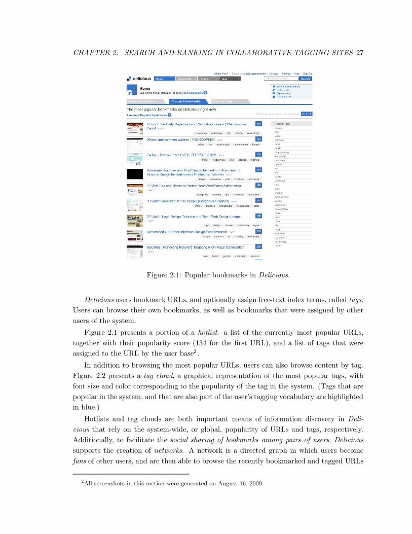
CHAPTER 2. SEARCH AND RANKING IN COLLABORATIVE TAGGING SITES 27
Figure 2.1: Popular bookmarks in Delicious.
Delicious users bookmark URLs, and optionally assign free-text index terms, called tags.
Users can browse their own bookmarks, as well as bookmarks that were assigned by other
users of the system.
Figure 2.1 presents a portion of a hotlist: a list of the currently most popular URLs,
together with their popularity score (134 for the first URL), and a list of tags that were
assigned to the URL by the user base2 .
In addition to browsing the most popular URLs, users can also browse content by tag.
Figure 2.2 presents a tag cloud, a graphical representation of the most popular tags, with
font size and color corresponding to the popularity of the tag in the system. (Tags that are
popular in the system, and that are also part of the user’s tagging vocabulary are highlighted
in blue.)
Hotlists and tag clouds are both important means of information discovery in Deli-
cious that rely on the system-wide, or global, popularity of URLs and tags, respectively.
Additionally, to facilitate the social sharing of bookmarks among pairs of users, Delicious
supports the creation of networks. A network is a directed graph in which users become
fans of other users, and are then able to browse the recently bookmarked and tagged URLs
2All screenshots in this section were generated on August 16, 2009.
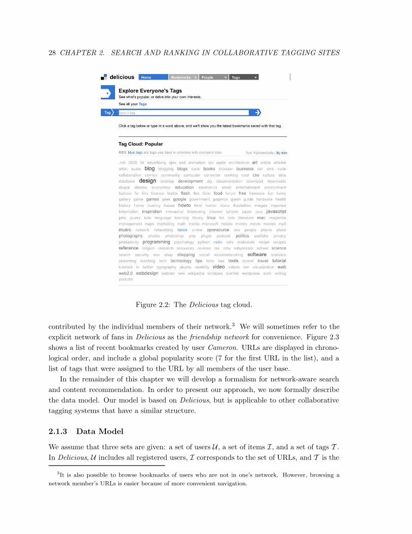
28 CHAPTER 2. SEARCH AND RANKING IN COLLABORATIVE TAGGING SITES
Figure 2.2: The Delicious tag cloud.
contributed by the individual members of their network.3 We will sometimes refer to the
explicit network of fans in Delicious as the friendship network for convenience. Figure 2.3
shows a list of recent bookmarks created by user Cameron. URLs are displayed in chrono-
logical order, and include a global popularity score (7 for the first URL in the list), and a
list of tags that were assigned to the URL by all members of the user base.
In the remainder of this chapter we will develop a formalism for network-aware search
and content recommendation. In order to present our approach, we now formally describe
the data model. Our model is based on Delicious, but is applicable to other collaborative
tagging systems that have a similar structure.
2.1.3 Data Model
We assume that three sets are given: a set of users U , a set of items I, and a set of tags T .
In Delicious, U includes all registered users, I corresponds to the set of URLs, and T is the
3It is also possible to browse bookmarks of users who are not in one’s network. However, browsing a
network member’s URLs is easier because of more convenient navigation.
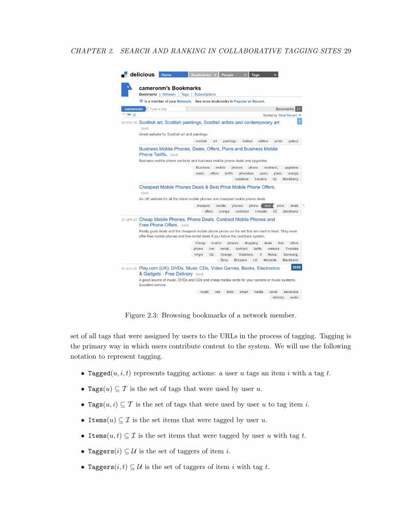
CHAPTER 2. SEARCH AND RANKING IN COLLABORATIVE TAGGING SITES 29
Figure 2.3: Browsing bookmarks of a network member.
set of all tags that were assigned by users to the URLs in the process of tagging. Tagging is
the primary way in which users contribute content to the system. We will use the following
notation to represent tagging.
• Tagged(u, i, t) represents tagging actions: a user u tags an item i with a tag t.
• Tags(u) ⊆ T is the set of tags that were used by user u.
• Tags(u, i) ⊆ T is the set of tags that were used by user u to tag item i.
• Items(u) ⊆ I is the set items that were tagged by user u.
• Items(u, t) ⊆ I is the set items that were tagged by user u with tag t.
• Taggers(i) ⊆ U is the set of taggers of item i.
• Taggers(i, t) ⊆ U is the set of taggers of item i with tag t.
30 CHAPTER 2. SEARCH AND RANKING IN COLLABORATIVE TAGGING SITES
An additional activity that is complementary to tagging is the users’ participation in
social networks. A social network is a directed graph, in which nodes are users, and edges
correspond to social ties between users. These ties may be explicit, such as friendship,
similar age group, or geographic proximity. An example of an explicit tie in Delicious is
when a user becomes a fan of another user. Social ties may also be implicit, and may be
derived through data analysis. An example of an implicit tie is shared interest in a topic,
and we will describe the semantics of shared interest in the following sections.
We use the following notation to represent a social network.
• Link(u, v) represents a directional relationship between two users u, v ∈ U , and de-
notes that there is an edge from u to v. For example, in Delicious such an edge may
denote that u is a fan of v.
• Network(u) ⊆ U is the set of neighbors of u that is, Network(u) = {v | Link(u, v)}.
2.1.4 Description of the Experimental Dataset
The methods described in this chapter were evaluated over a sample of Delicious to which
we were given access by the Delicious team. The dataset includes tagging actions during
a one-month period in 2006. In addition to tagging actions, our dataset also includes a
snapshot of the social network for the corresponding time period.
The dataset of tagging actions is very sparse and follows a long tail distribution [Kipp
and Campbell, 2006; Golder and Huberman, 2006]: most URLs are tagged by only a handful
of users, and many tags are only used by a few users. Sparse datasets are difficult to process
efficiently, and we applied the following procedure to reduce the size of the dataset. First,
we removed all URLs that were tagged by fewer than 10 distinct users. Additionally, we
removed tagging actions that include uncommon tags: only tags used by at least 4 distinct
users are included in our dataset. This cleaning procedure resulted in cutting the tail of
URLs and tags. As a result, the dataset was reduced to 27% of its original size. Our cleaned
dataset contains 116,177 distinct users who tagged 175,691 distinct URLs using 903 distinct
tags, for a total of 2,322,458 tagging actions.
Reduction of the dataset size was done primarily to allow us to store and access the
data more efficiently in a relational framework. However, while the size of the dataset was
reduced dramatically by our cleaning procedure, the effect of this reduction on keyword
search and content recommendation is limited. This is because only the URLs that were
“unpopular” over all tags and all users were removed. Each of the removed tags was
used by only a handful of Delicious users, and such tags have limited utility for content
recommendation and search. More often than not such uncommon tags form part of a user’s
private vocabulary, and are not intended for social sharing of information. Some examples
of such idiosyncratic tags are “Michael G’s birthday party” and “bug #1293”.
CHAPTER 2. SEARCH AND RANKING IN COLLABORATIVE TAGGING SITES 31
In the remainder of this chapter, we will focus on tagged URLs, and will neither explicitly
represent nor use URLs that are bookmarked but not tagged. Additionally, because we will
consider a user’s tagging to verify the effectiveness of content recommendation, and, in some
cases, to derive a social network, we focus our attention on taggers – users who contributed
at least one tagging action to the cleaned dataset.
2.1.5 Chapter Outline
In the first part of this chapter (Section 2.2), we study the effectiveness of several hotlist
generation strategies that take into account the user’s tagging behavior, social ties, and
interests. We conclude that leveraging context information significantly improves the quality
of content recommendation.
In the second part of this chapter (Sections 2.3 through 2.6), we develop a novel paradigm
of network-aware search, in which keyword search and ranking are executed over the content
that is recommended by the user’s network.
We review related work in Section 2.7 and conclude in Section 2.8.
2.2 Leveraging Semantic Context to Model User Interests
2.2.1 Introduction
In this section we study how the social context of a user can be used to improve the quality
of content recommendations. In Section 2.1.2 we described the basic types of context that
arise in collaborative tagging sites. In these sites users contribute content by tagging items,
forming social networks, and consuming content, primarily by browsing. An important
information discovery tool in collaborative tagging sites is a hotlist.
Hotlists are a means to expose vital content which has global popularity in the system.
An example of a hotlist is presented in Figure 2.1. However, while globally popular items
usually represent the consensus of many users, we experimentally observe in Section 2.2.3
that such items only account for a small fraction of any individual user’s interests. We thus
look for ways to account for user preferences during hotlist computation.
We first represent the interests of a user by the vocabulary he employs to tag URLs.
The intuition is that if a significant portion of the user’s tagging includes the tag “sports”,
the user is likely interested in sports-related content. This simple observation allows us to
replace a single global hotlist by per-tag lists, and to suggest potentially interesting URLs
by drawing from one or more per-tag lists in accordance with the user’s preferences. As we
demonstrate in Section 2.2.4, tag-driven customization significantly improves hotlist quality,
but its success is still limited by the global aspect.
In the second approach, we propose to model interest using social ties. These ties are
either explicitly stated or derived. An example of an explicit social tie is a network of fans.
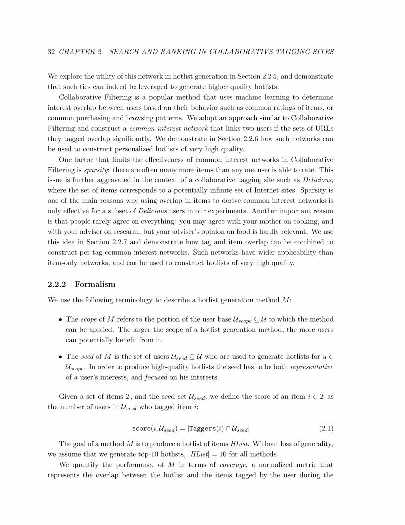
32 CHAPTER 2. SEARCH AND RANKING IN COLLABORATIVE TAGGING SITES
We explore the utility of this network in hotlist generation in Section 2.2.5, and demonstrate
that such ties can indeed be leveraged to generate higher quality hotlists.
Collaborative Filtering is a popular method that uses machine learning to determine
interest overlap between users based on their behavior such as common ratings of items, or
common purchasing and browsing patterns. We adopt an approach similar to Collaborative
Filtering and construct a common interest network that links two users if the sets of URLs
they tagged overlap significantly. We demonstrate in Section 2.2.6 how such networks can
be used to construct personalized hotlists of very high quality.
One factor that limits the effectiveness of common interest networks in Collaborative
Filtering is sparsity: there are often many more items than any one user is able to rate. This
issue is further aggravated in the context of a collaborative tagging site such as Delicious,
where the set of items corresponds to a potentially infinite set of Internet sites. Sparsity is
one of the main reasons why using overlap in items to derive common interest networks is
only effective for a subset of Delicious users in our experiments. Another important reason
is that people rarely agree on everything: you may agree with your mother on cooking, and
with your adviser on research, but your adviser’s opinion on food is hardly relevant. We use
this idea in Section 2.2.7 and demonstrate how tag and item overlap can be combined to
construct per-tag common interest networks. Such networks have wider applicability than
item-only networks, and can be used to construct hotlists of very high quality.
2.2.2 Formalism
We use the following terminology to describe a hotlist generation method M :
• The scope of M refers to the portion of the user base Uscope ⊆ U to which the method
can be applied. The larger the scope of a hotlist generation method, the more users
can potentially benefit from it.
• The seed of M is the set of users Useed ⊆ U who are used to generate hotlists for u ∈
Uscope. In order to produce high-quality hotlists the seed has to be both representative
of a user’s interests, and focused on his interests.
Given a set of items I, and the seed set Useed, we define the score of an item i ∈ I as
the number of users in Useed who tagged item i:
score(i,Useed) = |Taggers(i) ∩ Useed| (2.1)
The goal of a method M is to produce a hotlist of items HList. Without loss of generality,
we assume that we generate top-10 hotlists, |HList| = 10 for all methods.
We quantify the performance of M in terms of coverage, a normalized metric that
represents the overlap between the hotlist and the items tagged by the user during the
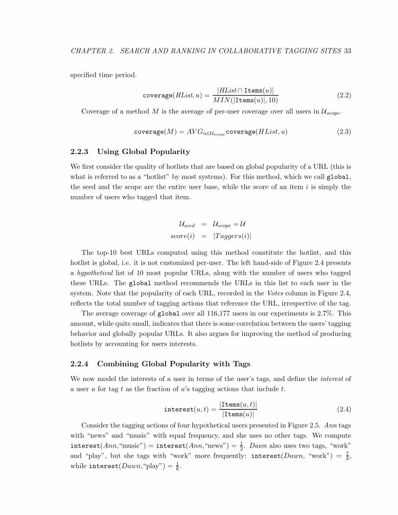
CHAPTER 2. SEARCH AND RANKING IN COLLABORATIVE TAGGING SITES 33
specified time period.
coverage(HList, u) =|HList ∩ Items(u)|
MIN(|Items(u)|, 10)(2.2)
Coverage of a method M is the average of per-user coverage over all users in Uscope.
coverage(M) = AV Gu∈Uscopecoverage(HList, u) (2.3)
2.2.3 Using Global Popularity
We first consider the quality of hotlists that are based on global popularity of a URL (this is
what is referred to as a “hotlist” by most systems). For this method, which we call global,
the seed and the scope are the entire user base, while the score of an item i is simply the
number of users who tagged that item.
Useed = Uscope = U
score(i) = |Taggers(i)|
The top-10 best URLs computed using this method constitute the hotlist, and this
hotlist is global, i.e. it is not customized per-user. The left hand-side of Figure 2.4 presents
a hypothetical list of 10 most popular URLs, along with the number of users who tagged
these URLs. The global method recommends the URLs in this list to each user in the
system. Note that the popularity of each URL, recorded in the Votes column in Figure 2.4,
reflects the total number of tagging actions that reference the URL, irrespective of the tag.
The average coverage of global over all 116,177 users in our experiments is 2.7%. This
amount, while quite small, indicates that there is some correlation between the users’ tagging
behavior and globally popular URLs. It also argues for improving the method of producing
hotlists by accounting for users interests.
2.2.4 Combining Global Popularity with Tags
We now model the interests of a user in terms of the user’s tags, and define the interest of
a user u for tag t as the fraction of u’s tagging actions that include t.
interest(u, t) =|Items(u, t)|
|Items(u)|(2.4)
Consider the tagging actions of four hypothetical users presented in Figure 2.5. Ann tags
with “news” and “music” with equal frequency, and she uses no other tags. We compute
interest(Ann,“music”) = interest(Ann,“news”) = 12 . Dawn also uses two tags, “work”
and “play”, but she tags with “work” more frequently: interest(Dawn, “work”) = 78 ,
while interest(Dawn,“play”) = 18 .
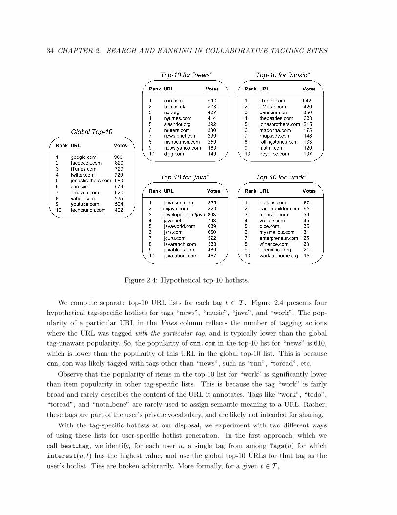
34 CHAPTER 2. SEARCH AND RANKING IN COLLABORATIVE TAGGING SITES
Figure 2.4: Hypothetical top-10 hotlists.
We compute separate top-10 URL lists for each tag t ∈ T . Figure 2.4 presents four
hypothetical tag-specific hotlists for tags “news”, “music”, “java”, and “work”. The pop-
ularity of a particular URL in the Votes column reflects the number of tagging actions
where the URL was tagged with the particular tag, and is typically lower than the global
tag-unaware popularity. So, the popularity of cnn.com in the top-10 list for “news” is 610,
which is lower than the popularity of this URL in the global top-10 list. This is because
cnn.com was likely tagged with tags other than “news”, such as “cnn”, “toread”, etc.
Observe that the popularity of items in the top-10 list for “work” is significantly lower
than item popularity in other tag-specific lists. This is because the tag “work” is fairly
broad and rarely describes the content of the URL it annotates. Tags like “work”, “todo”,
“toread”, and “nota bene” are rarely used to assign semantic meaning to a URL. Rather,
these tags are part of the user’s private vocabulary, and are likely not intended for sharing.
With the tag-specific hotlists at our disposal, we experiment with two different ways
of using these lists for user-specific hotlist generation. In the first approach, which we
call best tag, we identify, for each user u, a single tag from among Tags(u) for which
interest(u, t) has the highest value, and use the global top-10 URLs for that tag as the
user’s hotlist. Ties are broken arbitrarily. More formally, for a given t ∈ T ,
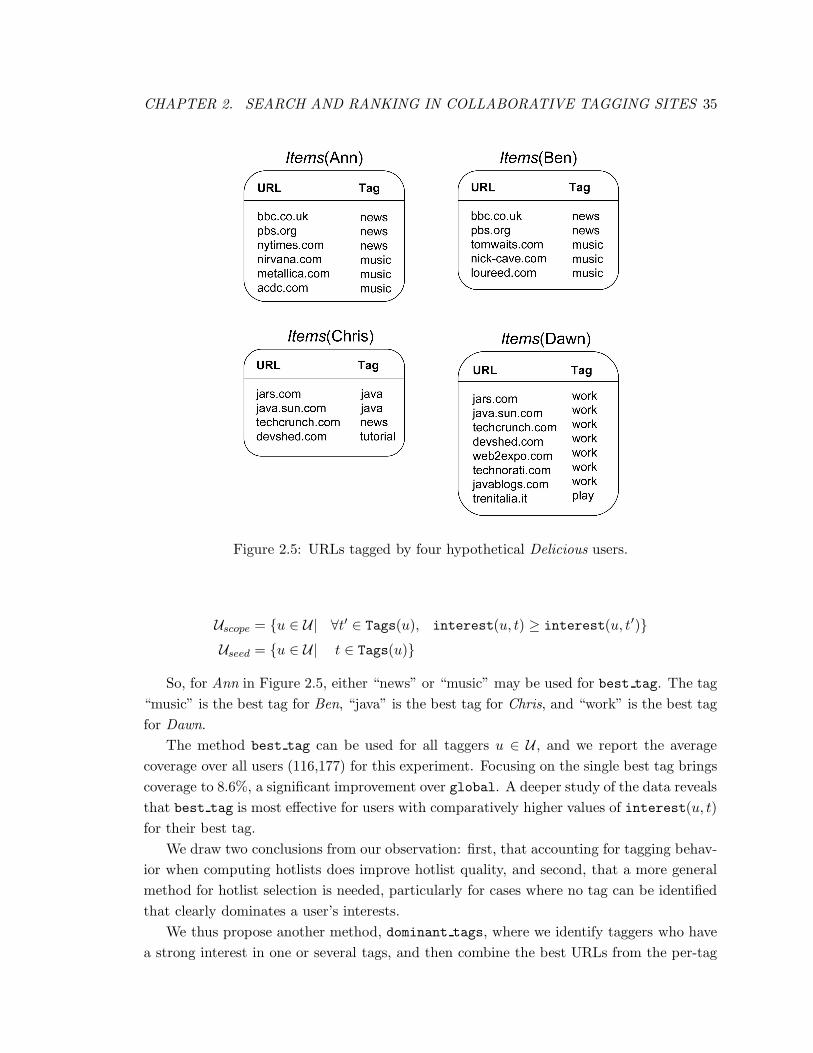
CHAPTER 2. SEARCH AND RANKING IN COLLABORATIVE TAGGING SITES 35
Figure 2.5: URLs tagged by four hypothetical Delicious users.
Uscope = {u ∈ U| ∀t′ ∈ Tags(u), interest(u, t) ≥ interest(u, t′)}
Useed = {u ∈ U| t ∈ Tags(u)}
So, for Ann in Figure 2.5, either “news” or “music” may be used for best tag. The tag
“music” is the best tag for Ben, “java” is the best tag for Chris, and “work” is the best tag
for Dawn.
The method best tag can be used for all taggers u ∈ U , and we report the average
coverage over all users (116,177) for this experiment. Focusing on the single best tag brings
coverage to 8.6%, a significant improvement over global. A deeper study of the data reveals
that best tag is most effective for users with comparatively higher values of interest(u, t)
for their best tag.
We draw two conclusions from our observation: first, that accounting for tagging behav-
ior when computing hotlists does improve hotlist quality, and second, that a more general
method for hotlist selection is needed, particularly for cases where no tag can be identified
that clearly dominates a user’s interests.
We thus propose another method, dominant tags, where we identify taggers who have
a strong interest in one or several tags, and then combine the best URLs from the per-tag
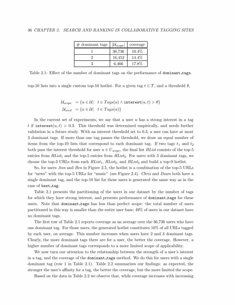
36 CHAPTER 2. SEARCH AND RANKING IN COLLABORATIVE TAGGING SITES
# dominant tags |Uscope| coverage
1 36,736 10.4%
2 16,452 14.4%
3 6,466 17.8%
Table 2.1: Effect of the number of dominant tags on the performance of dominant tags.
top-10 lists into a single custom top-10 hotlist. For a given tag t ∈ T , and a threshold θ,
Uscope = {u ∈ U| t ∈ Tags(u) ∧ interest(u, t) > θ}
Useed = {u ∈ U| t ∈ Tags(u)}
In the current set of experiments, we say that a user u has a strong interest in a tag
t if interest(u, t) > 0.3. This threshold was determined empirically, and needs further
validation in a future study. With an interest threshold set to 0.3, a user can have at most
3 dominant tags. If more than one tag passes the threshold, we draw an equal number of
items from the top-10 lists that correspond to each dominant tag. If two tags t1 and t2
both pass the interest threshold for user u ∈ Uscope, the final list HList consists of the top-5
entries from HList1 and the top-5 entries from HList2. For users with 3 dominant tags, we
choose the top-3 URLs from each HList1, HList2, and HList3 and build a top-9 hotlist.
So, for users Ann and Ben in Figure 2.5, the hotlist is a combination of the top-5 URLs
for “news” with the top-5 URLs for “music” (see Figure 2.4). Chris and Dawn both have a
single dominant tag, and the top-10 list for these users is generated the same way as in the
case of best tag.
Table 2.1 presents the partitioning of the users in our dataset by the number of tags
for which they have strong interest, and presents performance of dominant tags for these
users. Note that dominant tags has less than perfect scope: the total number of users
partitioned in this way is smaller than the entire user base; 49% of users in our dataset have
no dominant tags.
The first row of Table 2.1 reports coverage as an average over the 36,736 users who have
one dominant tag. For those users, the generated hotlist constitutes 10% of all URLs tagged
by each user, on average. This number increases when users have 2 and 3 dominant tags.
Clearly, the more dominant tags there are for a user, the better the coverage. However, a
higher number of dominant tags corresponds to a more limited scope of applicability.
We now turn our attention to the relationship between the strength of a user’s interest
in a tag, and the coverage of the dominant tags method. We do this for users with a single
dominant tag (row 1 in Table 2.1). Table 2.2 summarizes our findings: as expected, the
stronger the user’s affinity for a tag, the better the coverage, but the more limited the scope.
Based on the data in Table 2.2 we observe that, while coverage increases with increasing
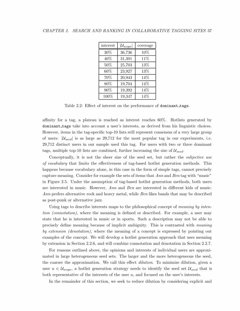
CHAPTER 2. SEARCH AND RANKING IN COLLABORATIVE TAGGING SITES 37
interest |Uscope| coverage
30% 36,736 10%
40% 31,391 11%
50% 25,703 13%
60% 23,927 13%
70% 20,943 14%
80% 19,704 14%
90% 19,392 14%
100% 19,347 14%
Table 2.2: Effect of interest on the performance of dominant tags.
affinity for a tag, a plateau is reached as interest reaches 60%. Hotlists generated by
dominant tags take into account a user’s interests, as derived from his linguistic choices.
However, items in the tag-specific top-10 lists still represent consensus of a very large group
of users: |Useed| is as large as 29,712 for the most popular tag in our experiments, i.e.
29,712 distinct users in our sample used this tag. For users with two or three dominant
tags, multiple top-10 lists are combined, further increasing the size of Useed.
Conceptually, it is not the sheer size of the seed set, but rather the subjective use
of vocabulary that limits the effectiveness of tag-based hotlist generation methods. This
happens because vocabulary alone, in this case in the form of simple tags, cannot precisely
capture meaning. Consider for example the sets of items that Ann and Ben tag with “music”
in Figure 2.5. Under the assumption of tag-based hotlist generation methods, both users
are interested in music. However, Ann and Ben are interested in different kids of music:
Ann prefers alternative rock and heavy metal, while Ben likes bands that may be described
as post-punk or alternative jazz.
Using tags to describe interests maps to the philosophical concept of meaning by inten-
tion (connotation), where the meaning is defined or described. For example, a user may
state that he is interested in music or in sports. Such a description may not be able to
precisely define meaning because of implicit ambiguity. This is contrasted with meaning
by extension (denotation), where the meaning of a concept is expressed by pointing out
examples of the concept. We will develop a hotlist generation approach that uses meaning
by extension in Section 2.2.6, and will combine connotation and denotation in Section 2.2.7.
For reasons outlined above, the opinions and interests of individual users are approxi-
mated in large heterogeneous seed sets. The larger and the more heterogeneous the seed,
the coarser the approximation. We call this effect dilution. To minimize dilution, given a
user u ∈ Uscope, a hotlist generation strategy needs to identify the seed set Useed that is
both representative of the interests of the user u, and focused on the user’s interests.
In the remainder of this section, we seek to reduce dilution by considering explicit and
38 CHAPTER 2. SEARCH AND RANKING IN COLLABORATIVE TAGGING SITES
implicit social ties between users during hotlist generation.
2.2.5 Computing Hotlists Using the Friendship Network
The goal of this experiment is to explore the utility of the explicit friendship network in
Delicious for hotlist generation. Of 116,177 taggers in our experiments, 36,248 (31%) also
have a social network, and we term such users friendly taggers. Choosing the friendship
network as Useed is justified by the fact that Delicious users tend to pay attention to their
friends tagging actions, which influence their own. In particular, users can subscribe to
feeds and get notified whenever one of the users in their network tags a new URL.
For each friendly tagger, we generate a customized hotlist by drawing 10 URLs with
highest popularity from among URLs tagged by the members of his network. We refer to
this hotlist generation method as friends. The scope of friends is the set of friendly
taggers, and the seed is defined, for a fixed user u, as the network of u.
Uscope = {u ∈ U | ∃v ∈ U : v ∈ Network(u)}
Useed = Network(u)
Consider again the hypothetical users in Figure 2.5, and suppose that Chris is a fan of
Ann and Ben, that is, Network(Chris) = {Ann,Ben}. Then the hotlist for Chris would
combine Items(Ann) and Items(Ben). In this list, bbc.co.uk and pbs.org would be
ranked higher than the other URLs, since these items each have two votes, while other
items each have one vote. Note that the coverage of the resulting hotlist with respect to
Items(Chris) is 0, signifying that, while Ann and Ben may be friends with Chris in real life,
Chris’s interests diverge from those of his friends. Suppose now that Chris is a fan of Dawn,
that is, Network(Chris) = {Dawn}. In this case the hotlist for Chris is Items(Dawn),
which attains a perfect coverage of 1. This example illustrates that explicitly declared
networks, such as a network of fans, may or may not be indicative of the users’ interests,
and we now demonstrate this experimentally.
We focus on a random subset of friendly taggers, 4,644 in all, for our experiments
in this section, and find the coverage of friends to be 42.9%, a significant improvement
over global, which was 3.3% for the sample of friendly taggers in our experiments. Note
that AV G(|Useed|) = 4 for our sample, multiple orders of magnitude less than for previous
methods.
We now explore how tagging can be used to deduce interest overlap among users, and
how such overlap can be used to generate hotlists of very high quality. We report two
experiments: in the first, two users are said to have a social tie if the sets of URLs they
tag overlap significantly; in the second, we enrich the set of derived ties by considering
tag-specific overlap in URLs.
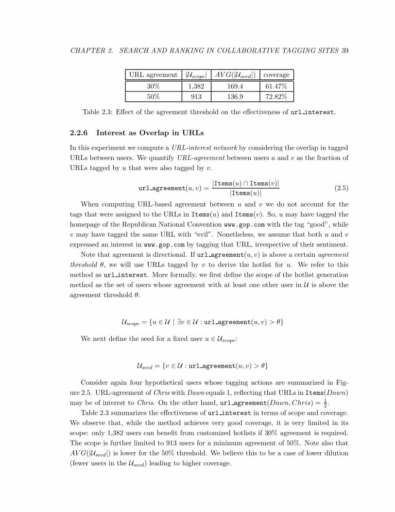
CHAPTER 2. SEARCH AND RANKING IN COLLABORATIVE TAGGING SITES 39
URL agreement |Uscope| AV G(|Useed|) coverage
30% 1,382 169.4 61.47%
50% 913 136.9 72.82%
Table 2.3: Effect of the agreement threshold on the effectiveness of url interest.
2.2.6 Interest as Overlap in URLs
In this experiment we compute a URL-interest network by considering the overlap in tagged
URLs between users. We quantify URL-agreement between users u and v as the fraction of
URLs tagged by u that were also tagged by v.
url agreement(u, v) =|Items(u) ∩ Items(v)|
|Items(u)|(2.5)
When computing URL-based agreement between u and v we do not account for the
tags that were assigned to the URLs in Items(u) and Items(v). So, u may have tagged the
homepage of the Republican National Convention www.gop.com with the tag “good”, while
v may have tagged the same URL with “evil”. Nonetheless, we assume that both u and v
expressed an interest in www.gop.com by tagging that URL, irrespective of their sentiment.
Note that agreement is directional. If url agreement(u, v) is above a certain agreement
threshold θ, we will use URLs tagged by v to derive the hotlist for u. We refer to this
method as url interest. More formally, we first define the scope of the hotlist generation
method as the set of users whose agreement with at least one other user in U is above the
agreement threshold θ:
Uscope = {u ∈ U | ∃v ∈ U : url agreement(u, v) > θ}
We next define the seed for a fixed user u ∈ Uscope:
Useed = {v ∈ U : url agreement(u, v) > θ}
Consider again four hypothetical users whose tagging actions are summarized in Fig-
ure 2.5. URL-agreement of Chris with Dawn equals 1, reflecting that URLs in Items(Dawn)
may be of interest to Chris. On the other hand, url agreement(Dawn,Chris) = 12 .
Table 2.3 summarizes the effectiveness of url interest in terms of scope and coverage.
We observe that, while the method achieves very good coverage, it is very limited in its
scope: only 1,382 users can benefit from customized hotlists if 30% agreement is required.
The scope is further limited to 913 users for a minimum agreement of 50%. Note also that
AV G(|Useed|) is lower for the 50% threshold. We believe this to be a case of lower dilution
(fewer users in the Useed) leading to higher coverage.
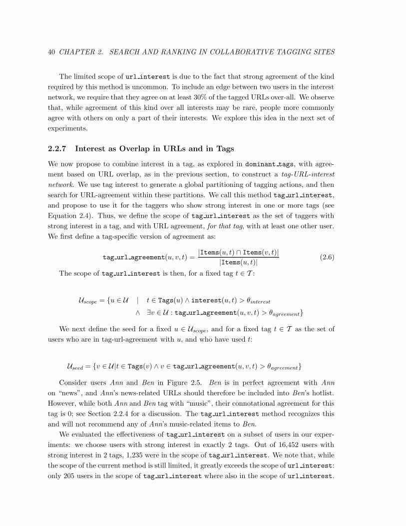
40 CHAPTER 2. SEARCH AND RANKING IN COLLABORATIVE TAGGING SITES
The limited scope of url interest is due to the fact that strong agreement of the kind
required by this method is uncommon. To include an edge between two users in the interest
network, we require that they agree on at least 30% of the tagged URLs over-all. We observe
that, while agreement of this kind over all interests may be rare, people more commonly
agree with others on only a part of their interests. We explore this idea in the next set of
experiments.
2.2.7 Interest as Overlap in URLs and in Tags
We now propose to combine interest in a tag, as explored in dominant tags, with agree-
ment based on URL overlap, as in the previous section, to construct a tag-URL-interest
network. We use tag interest to generate a global partitioning of tagging actions, and then
search for URL-agreement within these partitions. We call this method tag url interest,
and propose to use it for the taggers who show strong interest in one or more tags (see
Equation 2.4). Thus, we define the scope of tag url interest as the set of taggers with
strong interest in a tag, and with URL agreement, for that tag, with at least one other user.
We first define a tag-specific version of agreement as:
tag url agreement(u, v, t) =|Items(u, t) ∩ Items(v, t)|
|Items(u, t)|(2.6)
The scope of tag url interest is then, for a fixed tag t ∈ T :
Uscope = {u ∈ U | t ∈ Tags(u) ∧ interest(u, t) > θinterest
∧ ∃v ∈ U : tag url agreement(u, v, t) > θagreement}
We next define the seed for a fixed u ∈ Uscope, and for a fixed tag t ∈ T as the set of
users who are in tag-url-agreement with u, and who have used t:
Useed = {v ∈ U|t ∈ Tags(v) ∧ v ∈ tag url agreement(u, v, t) > θagreement}
Consider users Ann and Ben in Figure 2.5. Ben is in perfect agreement with Ann
on “news”, and Ann’s news-related URLs should therefore be included into Ben’s hotlist.
However, while both Ann and Ben tag with “music”, their connotational agreement for this
tag is 0; see Section 2.2.4 for a discussion. The tag url interest method recognizes this
and will not recommend any of Ann’s music-related items to Ben.
We evaluated the effectiveness of tag url interest on a subset of users in our exper-
iments: we choose users with strong interest in exactly 2 tags. Out of 16,452 users with
strong interest in 2 tags, 1,235 were in the scope of tag url interest. We note that, while
the scope of the current method is still limited, it greatly exceeds the scope of url interest:
only 205 users in the scope of tag url interest where also in the scope of url interest.
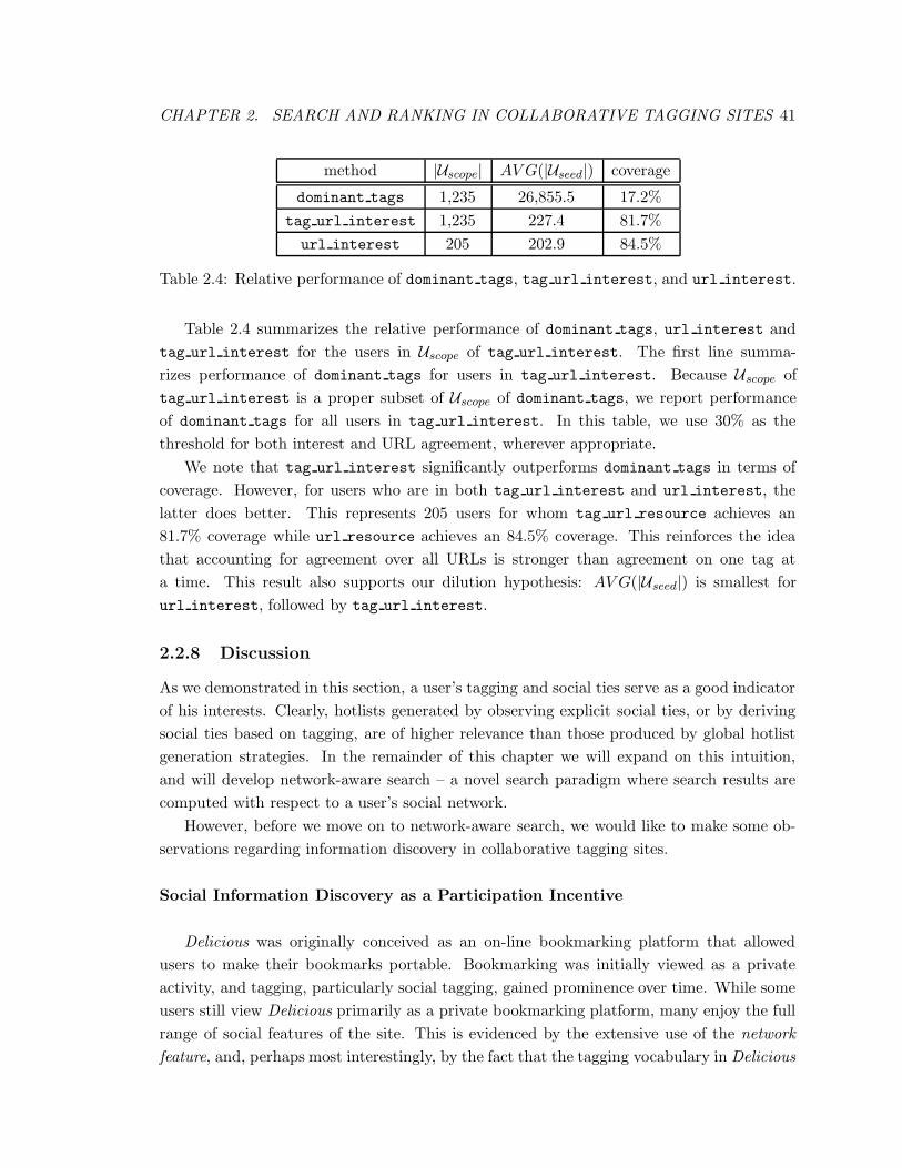
CHAPTER 2. SEARCH AND RANKING IN COLLABORATIVE TAGGING SITES 41
method |Uscope| AV G(|Useed|) coverage
dominant tags 1,235 26,855.5 17.2%
tag url interest 1,235 227.4 81.7%
url interest 205 202.9 84.5%
Table 2.4: Relative performance of dominant tags, tag url interest, and url interest.
Table 2.4 summarizes the relative performance of dominant tags, url interest and
tag url interest for the users in Uscope of tag url interest. The first line summa-
rizes performance of dominant tags for users in tag url interest. Because Uscope of
tag url interest is a proper subset of Uscope of dominant tags, we report performance
of dominant tags for all users in tag url interest. In this table, we use 30% as the
threshold for both interest and URL agreement, wherever appropriate.
We note that tag url interest significantly outperforms dominant tags in terms of
coverage. However, for users who are in both tag url interest and url interest, the
latter does better. This represents 205 users for whom tag url resource achieves an
81.7% coverage while url resource achieves an 84.5% coverage. This reinforces the idea
that accounting for agreement over all URLs is stronger than agreement on one tag at
a time. This result also supports our dilution hypothesis: AV G(|Useed|) is smallest for
url interest, followed by tag url interest.
2.2.8 Discussion
As we demonstrated in this section, a user’s tagging and social ties serve as a good indicator
of his interests. Clearly, hotlists generated by observing explicit social ties, or by deriving
social ties based on tagging, are of higher relevance than those produced by global hotlist
generation strategies. In the remainder of this chapter we will expand on this intuition,
and will develop network-aware search – a novel search paradigm where search results are
computed with respect to a user’s social network.
However, before we move on to network-aware search, we would like to make some ob-
servations regarding information discovery in collaborative tagging sites.
Social Information Discovery as a Participation Incentive
Delicious was originally conceived as an on-line bookmarking platform that allowed
users to make their bookmarks portable. Bookmarking was initially viewed as a private
activity, and tagging, particularly social tagging, gained prominence over time. While some
users still view Delicious primarily as a private bookmarking platform, many enjoy the full
range of social features of the site. This is evidenced by the extensive use of the network
feature, and, perhaps most interestingly, by the fact that the tagging vocabulary in Delicious
42 CHAPTER 2. SEARCH AND RANKING IN COLLABORATIVE TAGGING SITES
converged to form a folksonomy. A folksonomy is a vocabulary, along with a classification
system, that emerges in a bottom-up manner from the collaborative tagging practices of a
social group. Users who tag socially tend to use folksonomy terms in their tagging, enabling
other users to identify their content more easily.
In our work with the Delicious dataset we observed that participation in a network of
fans and social tagging are complementary activities: users who form social networks are
more likely to tag and vice versa 4 .
As we just discussed, many Delicious users contribute content in a socially aware manner.
Therefore, an important technical question, and one that may influence the very survival
of social tagging sites like Delicious, is how to support social information discovery. In
this section we described how a user’s social behavior may be leveraged to generate high-
quality hotlists, and we will present an algorithmic framework for network-aware search in
the remaining sections of this chapter. However, the scope of applicability of our methods
is limited to those users who choose to interact with the collaborative tagging platform
in a collaborative, social manner. We believe that supporting socially aware information
discovery will enrich the user experience, serving as a powerful incentive for continued user
participation. This will, in turn, increase the scope of applicability of our methods.
Finally, we remark that the distinction between private tagging that involves idiosyn-
cratic vocabulary, and public tagging that draws upon a folksonomy of terms, calls for the
study of privacy in the context of collaborative tagging sites.
External Factors that Influence Interest
There are different reasons why a user would bookmark a URL and use specific tags to
label it. Our evaluation of hotlist recommendation strategies shows that a user’s interest
in a URL is influenced by his social ties, many or all of which may be external: formed in
real life, in another social content site, etc. Another external influence over a user’s interest
in a URL or in a tag is the general popularity of that URL or tag. Bursts in interest have
been observed and studied in the past [Cohen and McCallum, 2003]. Indeed, some tags
appear at certain periods of time and indicate a trend in the general public or among a
community of users (e.g., people tend to visit travel sites more often during holiday time).
Wars, health, and news also tend to follow similar trends, while other tags, such as cooking
or professional photography, have a steadier popularity.
Persistence of Interest and Agreement
Collaborative Filtering is based on a strong underlying assumption that people who
4We do not provide actual figures here so as not to disclose Yahoo!’s sensitive statistics.
CHAPTER 2. SEARCH AND RANKING IN COLLABORATIVE TAGGING SITES 43
agreed in the past tend to agree again in the future, and conversely that items that are
similar will continue to be similarly liked or disliked by a given user. Consequently, existing
systems do little to detect or predict changes in user preferences. During our experimental
evaluation we found that the assumption of persistence of interest and agreement does not
always hold in Delicious. Derived social ties, particularly those based on resource agreement,
were rarely conserved from one time period to the next. We identified the short lifespan of
URLs as the main reason: many URLs are only tagged actively for a period of 1-2 weeks.
A promising direction for future work is incorporating time into the analysis of interest and
agreement. Another direction is to derive interest networks based on clusters of similar
URLs, rather than on individual URLs. A similar approach is taken in [Wu et al., 2006b],
in which the authors study the relationship between items, tags, and users in scope of a
unified probabilistic generative model.
2.3 Network-Aware Search
2.3.1 Introduction
In Section 2.1 we described collaborative tagging sites. These sites are gaining popularity,
and while browsing is still the predominant way of reaching content, ranked keyword-based
search will become more important as the size of networks and tagged content expand.
An important question that we address in the remainder of this chapter is how to support
network-aware search – a mechanism that will return the top-ranked answers to a query
consisting of a set of tags, given a user with a particular network. Such a mechanism is
important not only for supporting search within these sites, but also for incorporating a
user’s network and tagging behavior in general web search [Heymann et al., 2008].
Information Retrieval generally assumes content to be relatively static, while user in-
terests are dynamic, expressed via keyword queries [Baeza-Yates and Ribeiro-Neto, 1999].
On the other hand, the Publish/Subscribe model assumes static publisher needs and dy-
namic streaming content [Wu et al., 2006a]. In collaborative tagging sites, both content
and interest are dynamic. Users tag new photos on Flickr and new videos on YouTube
every day and develop interest in new topics. In the remainder of this chapter we model
collaborative tagging sites as follows: users in the system can be either taggers or seekers.
Taggers annotate items with one or more tags. A query is composed of a set of tags and
is asked by a seeker. A linking relation connects seekers and taggers, thereby forming the
network associated with each seeker. In practice the set of seekers and the set of taggers
may overlap, and our model and algorithms will not preclude this possibility.
Given a seeker, a network of taggers, and a query in the form of a set of tags, we wish
to return a ranked list of most relevant items. In Section 2.2 we demonstrated that a user’s
social context, expressed by his network and tagging, can be used to improve the quality of
content recommendation in collaborative tagging sites. In the remainder of this chapter, we
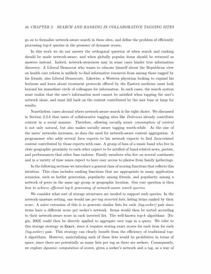
44 CHAPTER 2. SEARCH AND RANKING IN COLLABORATIVE TAGGING SITES
go on to formalize network-aware search in these sites, and define the problem of efficiently
processing top-k queries in the presence of dynamic scores.
In this work we do not answer the orthogonal question of when search and ranking
should be made network-aware, and when globally popular items should be returned as
answers instead. Indeed, network-awareness may in some cases hinder true information
discovery. A Liberal Democrat who wants to educate himself about the Republican view
on health care reform is unlikely to find informative resources from among those tagged by
his friends, also Liberal Democrats. Likewise, a Western physician looking to expand his
horizons and learn about treatment protocols offered by the Eastern medicine must look
beyond his immediate circle of colleagues for information. In such cases, the search system
must realize that the user’s information need cannot be satisfied when tapping the user’s
network alone, and must fall back on the content contributed by the user base at large for
results.
Nonetheless, cases abound where network-aware search is the right choice. We discussed
in Section 2.2.8 that users of collaborative tagging sites like Delicious already contribute
content in a social manner. Therefore, allowing socially aware consumption of content
is not only natural, but also makes socially aware tagging worth-while. As the size of
the users’ networks increases, so does the need for network-aware content aggregation. A
programmer who adds several Java experts to his network expects to find Java-related
content contributed by those experts with ease. A group of fans of a music band who live in
close geographic proximity to each other expect to be notified of band-related news, parties,
and performances that other fans endorse. Family members who live on several continents
and in a variety of time zones expect to have easy access to photos from family gatherings.
In the following sections we introduce a general class of scoring functions that reflects this
intuition. This class includes ranking functions that are appropriate in many application
scenarios, such as hotlist generation, popularity among friends, and popularity among a
network of peers in the same age group or geographic location. Our core question is then
how to achieve efficient top-k processing of network-aware search queries.
We consider what sort of storage structures are needed to support such queries. In the
network-unaware setting, one would use per-tag inverted lists, listing items ranked by their
score. A naive extension of this is to generate similar lists for each (tag,seeker) pair since
items have a different score per seeker’s network. Items would then be sorted according
to their network-aware score in each inverted list. The well-known top-k algorithms [Fa-
gin, 2002] could then be directly applied to aggregate over tags in a query. We refer to
this storage strategy as Exact, since it requires storing exact scores for each item for each
(tag,seeker) pair. This strategy can clearly benefit from the efficiency of traditional top-
k algorithms. However, materializing each of these lists would be prohibitive in terms of
space, since there are potentially as many lists per tag as there are seekers. Consequently,
we explore dynamic computation of scores, given a seeker’s network and a tag, as a way of
CHAPTER 2. SEARCH AND RANKING IN COLLABORATIVE TAGGING SITES 45
achieving a balance between processing time and storage space. Note that while traditional
top-k algorithms aggregate scores on different keywords at query time, they assume the
inverted lists are ordered by exact scores, even if exact scores of list entries are not avail-
able. The most straightforward dynamic approach materializes only per-tag inverted lists.
These inverted lists are seeker-independent, so their entries cannot contain exact per-seeker
scores but only upper-bounds for each item, i.e., its max score over all seekers. We refer
to this strategy as Global Upper-Bound. We develop generalizations of top-k processing
algorithms to incorporate network-aware search. In particular, we modify the classic NRA
(No Random Access) and TA (Threshold Algorithm) to account for score upper-bounds and
dynamic computation of exact scores (Section 2.4).
The Exact and Global Upper-Bound strategies represent two extremes in the space-
time trade-off. While Global Upper-Bound will offer considerable savings in space, we
expect query processing to take much longer, since the upper-bounds may be very coarse.
The finer the upper-bounds, the closer they are to exact scores for a given seeker, which
affects the order of entries in the inverted lists. We explore two refinements in Section 2.5.
Our first refinement identifies groups of seekers whose “network-aware” scores are close.
The score upper-bound computed for such a group will then be tighter than the global
upper-bound. These groups represent seekers who exhibit similar networking behavior.
We refer to this strategy as Cluster-Seekers. This strategy leads to one inverted list per
(tag,cluster) pair. At query time, we find the (tag,cluster) inverted lists associated with that
seeker and aggregate over them. We will see that the Cluster-Seekers strategy performs
faster than Global Upper-Bound and consumes less space than Exact.
The performance of Cluster-Seekers depends on finding good clusterings. We explore
quality metrics that measure how well the order of entries in a per-cluster inverted list
reflects their order in a seeker-specific inverted list, for seekers who belong to that cluster.
Next, we explore Cluster-Taggers, a strategy that aims to group taggers in networks
based on similarity in their tagging behavior. Each tagger cluster is associated with an
inverted list, where items are ranked by their upper-bound within the cluster of taggers. At
query time, we determine the tagger clusters associated with a given seeker and compute
scores by aggregating over the inverted lists associated with these tagger clusters. Taggers
in a seeker’s network may belong to different clusters, and so multiple inverted lists per tag
may be relevant for a given seeker. We thus may have to aggregate over a larger number
of inverted lists, albeit with tighter upper-bounds per list. In our experiments, which we
present in Section 2.6, we found that Cluster-Taggers imposes little space penalty com-
pared to Global Upper-Bound, and outperforms Cluster-Seekers in both space overhead
and query time. However, not every seeker will benefit from this approach.
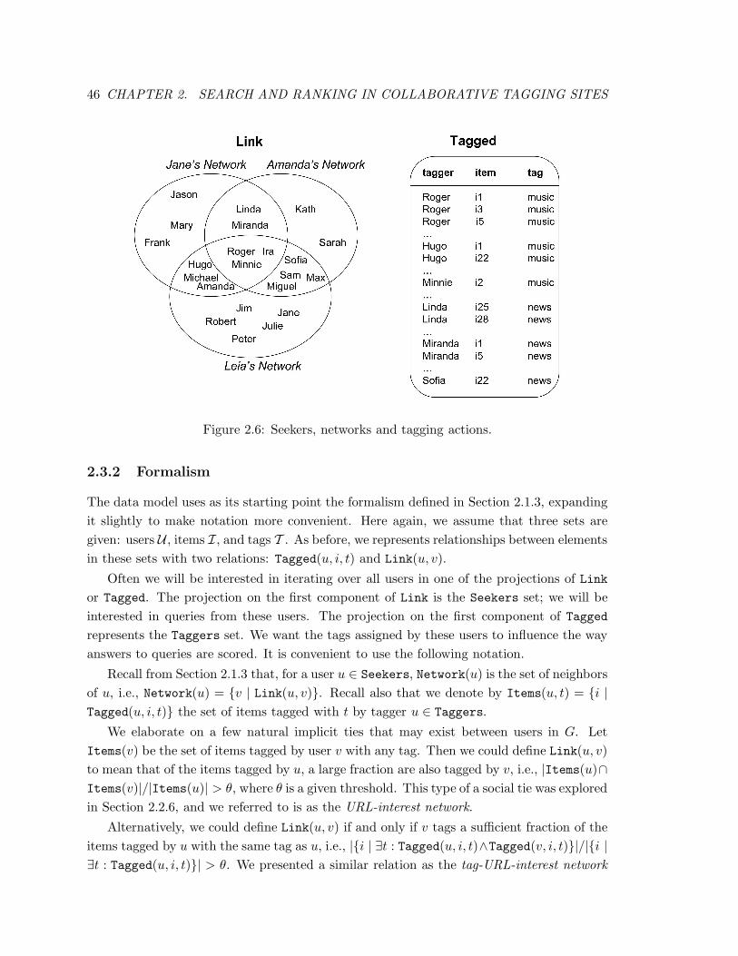
46 CHAPTER 2. SEARCH AND RANKING IN COLLABORATIVE TAGGING SITES
Figure 2.6: Seekers, networks and tagging actions.
2.3.2 Formalism
The data model uses as its starting point the formalism defined in Section 2.1.3, expanding
it slightly to make notation more convenient. Here again, we assume that three sets are
given: users U , items I, and tags T . As before, we represents relationships between elements
in these sets with two relations: Tagged(u, i, t) and Link(u, v).
Often we will be interested in iterating over all users in one of the projections of Link
or Tagged. The projection on the first component of Link is the Seekers set; we will be
interested in queries from these users. The projection on the first component of Tagged
represents the Taggers set. We want the tags assigned by these users to influence the way
answers to queries are scored. It is convenient to use the following notation.
Recall from Section 2.1.3 that, for a user u ∈ Seekers, Network(u) is the set of neighbors
of u, i.e., Network(u) = {v | Link(u, v)}. Recall also that we denote by Items(u, t) = {i |
Tagged(u, i, t)} the set of items tagged with t by tagger u ∈ Taggers.
We elaborate on a few natural implicit ties that may exist between users in G. Let
Items(v) be the set of items tagged by user v with any tag. Then we could define Link(u, v)
to mean that of the items tagged by u, a large fraction are also tagged by v, i.e., |Items(u)∩
Items(v)|/|Items(u)| > θ, where θ is a given threshold. This type of a social tie was explored
in Section 2.2.6, and we referred to is as the URL-interest network.
Alternatively, we could define Link(u, v) if and only if v tags a sufficient fraction of the
items tagged by u with the same tag as u, i.e., |{i | ∃t : Tagged(u, i, t)∧Tagged(v, i, t)}|/|{i |
∃t : Tagged(u, i, t)}| > θ. We presented a similar relation as the tag-URL-interest network
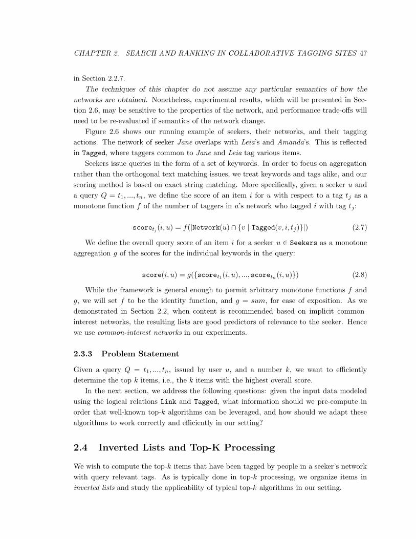
CHAPTER 2. SEARCH AND RANKING IN COLLABORATIVE TAGGING SITES 47
in Section 2.2.7.
The techniques of this chapter do not assume any particular semantics of how the
networks are obtained. Nonetheless, experimental results, which will be presented in Sec-
tion 2.6, may be sensitive to the properties of the network, and performance trade-offs will
need to be re-evaluated if semantics of the network change.
Figure 2.6 shows our running example of seekers, their networks, and their tagging
actions. The network of seeker Jane overlaps with Leia’s and Amanda’s. This is reflected
in Tagged, where taggers common to Jane and Leia tag various items.
Seekers issue queries in the form of a set of keywords. In order to focus on aggregation
rather than the orthogonal text matching issues, we treat keywords and tags alike, and our
scoring method is based on exact string matching. More specifically, given a seeker u and
a query Q = t1, ..., tn, we define the score of an item i for u with respect to a tag tj as a
monotone function f of the number of taggers in u’s network who tagged i with tag tj :
scoretj (i, u) = f(|Network(u) ∩ {v | Tagged(v, i, tj)}|) (2.7)
We define the overall query score of an item i for a seeker u ∈ Seekers as a monotone
aggregation g of the scores for the individual keywords in the query:
score(i, u) = g({scoret1(i, u), ..., scoretn(i, u)}) (2.8)
While the framework is general enough to permit arbitrary monotone functions f and
g, we will set f to be the identity function, and g = sum, for ease of exposition. As we
demonstrated in Section 2.2, when content is recommended based on implicit common-
interest networks, the resulting lists are good predictors of relevance to the seeker. Hence
we use common-interest networks in our experiments.
2.3.3 Problem Statement
Given a query Q = t1, ..., tn, issued by user u, and a number k, we want to efficiently
determine the top k items, i.e., the k items with the highest overall score.
In the next section, we address the following questions: given the input data modeled
using the logical relations Link and Tagged, what information should we pre-compute in
order that well-known top-k algorithms can be leveraged, and how should we adapt these
algorithms to work correctly and efficiently in our setting?
2.4 Inverted Lists and Top-K Processing
We wish to compute the top-k items that have been tagged by people in a seeker’s network
with query relevant tags. As is typically done in top-k processing, we organize items in
inverted lists and study the applicability of typical top-k algorithms in our setting.
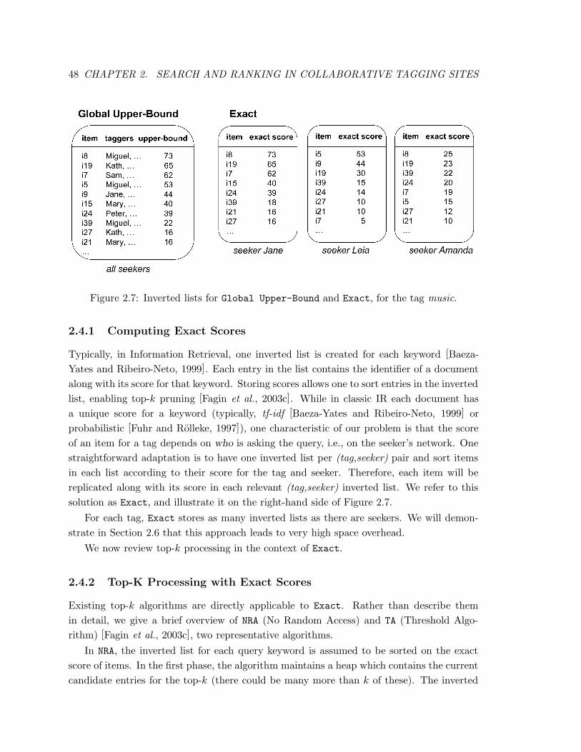
48 CHAPTER 2. SEARCH AND RANKING IN COLLABORATIVE TAGGING SITES
Figure 2.7: Inverted lists for Global Upper-Bound and Exact, for the tag music.
2.4.1 Computing Exact Scores
Typically, in Information Retrieval, one inverted list is created for each keyword [Baeza-
Yates and Ribeiro-Neto, 1999]. Each entry in the list contains the identifier of a document
along with its score for that keyword. Storing scores allows one to sort entries in the inverted
list, enabling top-k pruning [Fagin et al., 2003c]. While in classic IR each document has
a unique score for a keyword (typically, tf-idf [Baeza-Yates and Ribeiro-Neto, 1999] or
probabilistic [Fuhr and Rolleke, 1997]), one characteristic of our problem is that the score
of an item for a tag depends on who is asking the query, i.e., on the seeker’s network. One
straightforward adaptation is to have one inverted list per (tag,seeker) pair and sort items
in each list according to their score for the tag and seeker. Therefore, each item will be
replicated along with its score in each relevant (tag,seeker) inverted list. We refer to this
solution as Exact, and illustrate it on the right-hand side of Figure 2.7.
For each tag, Exact stores as many inverted lists as there are seekers. We will demon-
strate in Section 2.6 that this approach leads to very high space overhead.
We now review top-k processing in the context of Exact.
2.4.2 Top-K Processing with Exact Scores
Existing top-k algorithms are directly applicable to Exact. Rather than describe them
in detail, we give a brief overview of NRA (No Random Access) and TA (Threshold Algo-
rithm) [Fagin et al., 2003c], two representative algorithms.
In NRA, the inverted list for each query keyword is assumed to be sorted on the exact
score of items. In the first phase, the algorithm maintains a heap which contains the current
candidate entries for the top-k (there could be many more than k of these). The inverted
CHAPTER 2. SEARCH AND RANKING IN COLLABORATIVE TAGGING SITES 49
lists are scanned sequentially in parallel. When a new entry is found, it is added to the heap
along with its partial (exact) score. If the item was seen before, its score in the heap entry
is updated. For every heap entry, a worst-case score and a best-case score is maintained.
The worst-case score is based on the assumption that the item does not appear in those
lists where it is so far unseen. The best-case score assumes that the item’s score in a list
where it is unseen equals the bottom score of the heap (for that list). Items in the heap are
sorted on their worst-case score, with ties broken using best-case scores, and subsequent
ties broken arbitrarily. The algorithm stops when none of the entries outside of the top-k
items examined so far has a best-case score higher than the worst-case score of the kth item
in the buffer. The output of NRA consists of the set of top-k items in the buffer, for which
we have only partial score and hence no rank information. Subsequent work (e.g., [Ilyas et
al., 2002]) has adapted NRA so as to obtain exact rank information.
NRA can be directly applied in the context of Exact by picking the lists which correspond
to the current seeker and query keywords and aggregating over them as described above.
In TA, the inverted lists are sorted on score as for NRA, but random access is assumed in
addition to sequential access. The algorithm accesses items in the various lists sequentially,
and the lists are processed in parallel. TA maintains a heap, where items are kept sorted on
their complete score. When a new entry is seen in any list under sequential access, its scores
from other lists are obtained by random access. If its overall score is more than the score of
the kth entry in the heap, the items are swapped. Otherwise this new entry is discarded. At
any stage, the bottom score (seen under sequential access) is maintained for every list and
is used to compute a threshold. No unseen item can have a score higher than the threshold,
so if the score of the kth highest heap entry is greater than or equal to the threshold, then
the algorithm stops. The output consists of the top-k list in the buffer, including items
and their scores (and hence their ranks). Unlike in NRA, a far smaller portion of the lists
needs to be explored, and the heap never needs to contain more than k items. However,
this comes at the price of potentially many more random accesses.
TA can be applied directly in the context of Exact.
We now turn to describing our space-saving strategy and how top-k processing is adapted
to fit it.
2.4.3 Computing Score Upper-Bounds
In order to save space in storing inverted lists, we factor out the seeker from each per-tag
list and maintain entries of the form (item,taggers) where taggers are all taggers who tagged
the item with the tag. In this case, every item is stored at most once in the inverted list for
a given tag, as opposed to being replicated potentially once for each seeker. The question
now is which score to store with each entry. The answer to this question will determine
how the lists are ordered. Since scores are used for top-k pruning, it is safe to store, in
each per-tag inverted list, the maximum score that an item could have for the tag across all
50 CHAPTER 2. SEARCH AND RANKING IN COLLABORATIVE TAGGING SITES
possible seekers. We refer to such maximum score as the score upper-bound. Given a query
keyword tj, the score upper-bound of an item i for tj can be expressed as:
ub(i, tj) = MAXu∈Seekers|{v | Tagged(v, i, tj)} ∧ v ∈ Network(u)|
In other words, the score upper-bound is the highest score an item could have for a tag.
We refer to an inverted list organization based on these ideas as the Global Upper-Bound
strategy. We will assume that the inverted lists are supplemented by the Link relation
indexed by the seeker and the Tagged relation indexed by tag and item; these will support
our equivalent of random access. They also support efficient computation of exact scores,
given a seeker and an item.
Figure 2.7 shows the inverted list for tag music according to the Global Upper-Bound
strategy and its counter-part in Exact. Notice that Exact may store one item multiple
times across lists (e.g., item i19 is stored with seekers Jane, Amanda, and Leia). In the case
of Global Upper-Bound, an item is stored only once with its highest score (e.g., the score
of item i19 in Global Upper-Bound is higher than its score in the lists of Leia and Amanda
since it corresponds to its score for Jane). While the per-seeker inverted lists in Exact are
shorter than in Global Upper-Bound, the overall space consumption of Exact is expected
to be much higher. However, the relative ordering of items in the inverted list for Global
Upper-Bound does not necessarily reflect that of any per-seeker order in Exact (e.g., i19
is scored lower than i5 in Leia’s list while it is scored higher in the Global Upper-Bound
list). This may cause Global Upper-Bound to scan many more entries in the inverted lists
than Exact, thereby increasing query processing time. We next describe adaptations of NRA
and TA that use score bounds; their application to the bounds in Global Upper-Bound will
serve as another baseline (for processing time) in our experiments.
2.4.4 Top-k Processing with Score Upper-Bounds
We assume a function that does a “local aggregation”, taking a seeker and a pair (item,
taggers) from an inverted list and calculating the number of taggers that are friends of the
seeker. We also assume a function computeExactScore(i, u, tj) that computes the value of
Equation 2.8 by both retrieving the taggers of item i (for tag tj) and counting the number
of friends of u who tagged with tj. Such a function can be implemented as a SQL aggregate
query over the join of Link and Tagged.
2.4.4.1 NRA Generalization
Algorithm 1 shows the pseudo-code of gNRA. For any query, the inverted lists (ILt) corre-
sponding to each query keyword t are identified and are accessed sequentially in parallel,
using a criterion such as round-robin. When an item is encountered in a list, we: (i) record
the upper-bound of the item and (ii) compute the exact score of the item for that tag using
CHAPTER 2. SEARCH AND RANKING IN COLLABORATIVE TAGGING SITES 51
the taggers component of the IL entry. If the item has not been previously encountered, it
is added to the heap along with its score. If it is already in the heap, the score is updated.
Thus scores of items in the heap are partial exact scores and correspond to the notion of
worst-case score of classic NRA. The set of bottom (i.e., last seen) bounds of the lists is used
to compute best-case scores of items: for any item, its best-case score is the sum of its
partial exact score and the bottom bounds of all lists where the item has not been seen. If
an item is unseen anywhere, its partial exact score is 0 and its best-case score is the sum
of bottom bounds over all lists. The heap is kept sorted on the worst-case score, with ties
broken using best-case score, and then arbitrarily. The stopping condition is similar to that
for classic NRA: none of the items outside the top-k of the heap has a best-case score that
is more than the kth item’s worst-case score. However, for classic NRA, it is sufficient to
compare the kth item’s worst-case score in the heap with the largest best-case score of an
item in the heap outside of the top-k items. In our case, this would not be sound, since the
lists are only sorted on bounds, not necessarily on scores. Thus, a completely unseen item
can have a best-case score higher than the largest best-case score in the heap. Thus, we
compare the maximum of the largest best-case score outside of top-k in the heap and the
sum of all bottom bounds with the worst-case score of the kth item in the heap, stopping
when the latter is higher.
Algorithm 1: Bounds-Based NRA Algorithm (gNRA)
Require: seeker u, Query Q;
1: Open inverted lists ILt for each keyword t ∈ Q;
2: while worstcase(kth heap item) ≤ max{BestcaseUnseen, max{bestcase(j) | j ∈ heap− top-k}}
do
3: Get next list ILt using round-robin;
4: Get entry e = (i, ub, taggers) in ILt;
5: Update the bottom bound of ILt;
6: Compute partial exact score of i for t using itemTaggers;
7: If i is not in heap add it, otherwise update its partial exact score;
8: Update best-case scores of items in heap, and re-order heap;
9: BestcaseUnseen = sum of bottom bounds over all lists;
10: end while
11: Return top-k set of items from heap.
At this point, we are guaranteed that the set of items in the top-k of the heap belong
to the final top-k list. If the exact score (and rank) is of interest, we need to compute the
exact score of items in the heap on those lists where they are not seen. We can do this
by computing exact scores (our analog of Random Access) for the remaining terms of the
top-k heap items. 5
5Thus, gNRA in our setting is really “generalized Not many Random Accesses”.
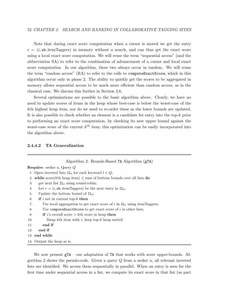
52 CHAPTER 2. SEARCH AND RANKING IN COLLABORATIVE TAGGING SITES
Note that during exact score computation when a cursor is moved we get the entry
e = (i, ub, itemTaggers) in memory without a search, and can thus get the exact score
using a local exact score computation. We will reuse the term “sequential access” (and the
abbreviation SA) to refer to the combination of advancement of a cursor and local exact
score computation. In our algorithm, these two always occur in tandem. We will reuse
the term “random access” (RA) to refer to the calls to computeExactScore, which in this
algorithm occur only in phase 2. The ability to quickly get the scores to be aggregated in
memory allows sequential access to be much more efficient than random access, as in the
classical case. We discuss this further in Section 2.6.
Several optimizations are possible to the basic algorithm above. Clearly, we have no
need to update scores of items in the heap whose best-case is below the worst-case of the
kth highest heap item, nor do we need to re-order these as the lower bounds are updated.
It is also possible to check whether an element is a candidate for entry into the top-k prior
to performing an exact score computation, by checking its new upper bound against the
worst-case score of the current kth item; this optimization can be easily incorporated into
the algorithm above.
2.4.4.2 TA Generalization
Algorithm 2: Bounds-Based TA Algorithm (gTA)
Require: seeker u, Query Q
1: Open inverted lists ILt for each keyword t ∈ Q;
2: while score(kth heap item) ≤ sum of bottom bounds over all lists do
3: get next list ILt using round-robin;
4: Let e = (i, ub, itemTaggers) be the next entry in ILt;
5: Update the bottom bound of ILt;
6: if i not in current top-k then
7: Use local aggregation to get exact score of i in ILt using itemTaggers;
8: Use computeExactScore to get exact score of i in other lists;
9: if i’s overall score > kth score in heap then
10: Swap kth item with i; keep top-k heap sorted;
11: end if
12: end if
13: end while
14: Output the heap as is.
We now present gTA – our adaptation of TA that works with score upper-bounds. Al-
gorithm 2 shows the pseudo-code. Given a query Q from a seeker u, all relevant inverted
lists are identified. We access them sequentially in parallel. When an entry is seen for the
first time under sequential access in a list, we compute its exact score in that list (as part
CHAPTER 2. SEARCH AND RANKING IN COLLABORATIVE TAGGING SITES 53
of SA) and perform exact score computations on the other lists (a set of RAs). Thus, we
always have complete exact scores for the items in the buffer. For each list, we remember
the bottom bound seen. The threshold is the sum of the bottom bounds over all lists. The
algorithm stops whenever the score of the kth item in the heap, which is kept sorted on
score, is no less than the threshold. At this stage, we can output the top-k items together
with their scores and hence rank them.
As with gNRA, there are slight modifications that can save accesses: when we find a new
item i we could iteratively retrieve scores in other lists, curtailing the iteration if we find
that the best-case of i is below the exact score of the kth item in the heap.
To summarize, both variants of Global Upper-Bound (gNRA and gTA) differ from Exact
in that the former needs to compute the exact score of an item for a tag and seeker at
query time. Using a simple variation of the argument in [Fagin et al., 2003c], we can show
that both Global Upper-Bound variants are instance optimal over all algorithms that use
the same upper-bound based storage. In the case of gTA, this means that gTA based on a
round-robin choice of cursors uses no more sequential accesses than any other “reasonable”
algorithm, up to a linear factor. Reasonable here means that the algorithms cannot make
a call to computeExactScore for an item until the item has been reached under sequential
access. This is the analog of the “no wild guesses” restriction of [Fagin et al., 2003c]. Similar
statements can be made for gNRA: Algorithm 1 is optimal, up to a constant factor, in number
of sequential accesses made, over algorithms that perform only sequential accesses. If we
consider the optimization where exact score computations are done only for items that have
a best-case score above the current kth highest-score, we find that it is optimal in terms of
the number of exact score computations.
However, any of these optimality statements only justify the use of these query process-
ing algorithms once a storage structure is fixed; they do not justify the storage structures
themselves. The accuracy of upper-bounds in the inverted list is clearly the key factor in the
efficiency of top-k pruning. The finer the upper-bound, the closer it is to the item’s exact
score and the faster an item can be pruned. Therefore, we need to explore further optimiza-
tions of our inverted list storage strategies. The clustering-based approaches introduced in
the next section work by identifying upper-bound based inverted lists for a (query,seeker)
pair and then applying either gNRA or gTA. They will differ on which lists are identified and
on how the clusters are formed.
2.5 Clustering and Query Processing
As discussed in Section 2.4, the greater the difference between the score upper-bound and
the exact score of an item for a tag, the more processing may be required to return the top k
results for a given (seeker,query) pair. The aim of this section is to describe methods which
reduce the difference between exact scores and upper-bounds by refining upper-bounds. The
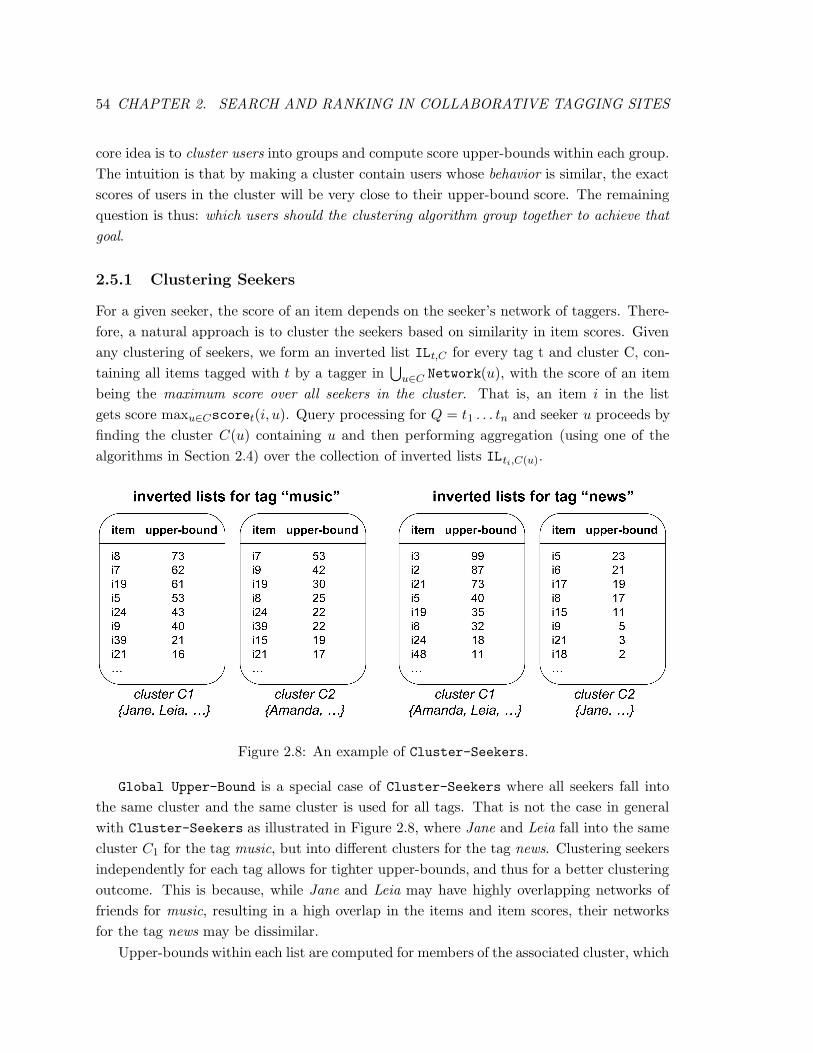
54 CHAPTER 2. SEARCH AND RANKING IN COLLABORATIVE TAGGING SITES
core idea is to cluster users into groups and compute score upper-bounds within each group.
The intuition is that by making a cluster contain users whose behavior is similar, the exact
scores of users in the cluster will be very close to their upper-bound score. The remaining
question is thus: which users should the clustering algorithm group together to achieve that
goal.
2.5.1 Clustering Seekers
For a given seeker, the score of an item depends on the seeker’s network of taggers. There-
fore, a natural approach is to cluster the seekers based on similarity in item scores. Given
any clustering of seekers, we form an inverted list ILt,C for every tag t and cluster C, con-
taining all items tagged with t by a tagger in⋃
u∈C Network(u), with the score of an item
being the maximum score over all seekers in the cluster. That is, an item i in the list
gets score maxu∈Cscoret(i, u). Query processing for Q = t1 . . . tn and seeker u proceeds by
finding the cluster C(u) containing u and then performing aggregation (using one of the
algorithms in Section 2.4) over the collection of inverted lists ILti,C(u).
Figure 2.8: An example of Cluster-Seekers.
Global Upper-Bound is a special case of Cluster-Seekers where all seekers fall into
the same cluster and the same cluster is used for all tags. That is not the case in general
with Cluster-Seekers as illustrated in Figure 2.8, where Jane and Leia fall into the same
cluster C1 for the tag music, but into different clusters for the tag news. Clustering seekers
independently for each tag allows for tighter upper-bounds, and thus for a better clustering
outcome. This is because, while Jane and Leia may have highly overlapping networks of
friends for music, resulting in a high overlap in the items and item scores, their networks
for the tag news may be dissimilar.
Upper-bounds within each list are computed for members of the associated cluster, which
CHAPTER 2. SEARCH AND RANKING IN COLLABORATIVE TAGGING SITES 55
makes the bounds necessarily tighter. For example, item i7 has a tighter upper-bound in
cluster C2 for tag music than in Global Upper-Bound in Figure 2.7. It is necessary to
compute seekers’ clusters on a per-tag basis in order to reflect (i) the overlap in networks
among different seekers and (ii) the overlap in tagging actions of taggers in clusters. Indeed,
if we generated a set of clusters which are agnostic to the tags, we could end up creating a
cluster containing Jane, Leia and Amanda (since they share some taggers in their networks).
The score upper-bounds for such a cluster would be coarser (e.g., i19 would have a score
upper-bound equal to 65 for tag news while it is equal to 30 in C2!).
One can easily show that, for single keyword queries, as we refine the clustering, the up-
per bounds can only get tighter, and hence the processing time of the generalized threshold
algorithms of the previous section can only go down, regardless of the seeker. In partic-
ular, Exact is optimal over all algorithms that use Cluster-Seekers, for any clustering,
assuming single-keyword queries.
For multi-keyword queries, clustering, while resulting in tighter upper-bounds, may not
always improve processing time. Consider a seeker u and a top-1 query Q = t1, t2. Assume
that, for this seeker, the lists of scores for the two keywords are ILt1,u = (x:10, i1:3, i2:2, . . .),
where the . . . is a long tail of scores below 2; ILt2,u = (i′1:20, i′2:19, . . . , i
′1000:19, . . . , x:15).
Suppose a clustering puts this seeker in her own cluster, thus making the bounds exact
for her! Under gNRA, we would have to keep making sequential accesses until we reach the
entry x:15 in the second list. However, it is possible that in Global Upper-Bound (the
coarsest possible clustering), the global inverted lists for the two keywords are: ILt1 =
(x:10, i1:3, i2:2, . . .); ILt2 = (x:22, i′1:20, i′2:19, . . . , i
′1000:19). The entry x might have a much
coarser (i.e., higher) bound in Global Upper-Bound and hence may bubble to the top of
the second list. Now, gNRA, after one round-robin, gets the full exact score of x (still 25 for
u). After this the algorithm will stop, since this score is higher than the sum of all bottom
scores. This example shows that an ideal clustering would take into account both the scores
and the ordering.
How do we cluster seekers? Ideally, we would find clusters that are optimal for the
running time of one of our algorithms in Section 2.4. However, as we show in [Amer-Yahia
et al., 2008a], finding a clustering that would minimize the worst-case running time over all
users is NP-hard. We also show that finding a clustering that minimizes the average-case
running time is NP-hard.
Given these complexity results, we must rely on heuristic methods to find clusters of
seekers. One natural approach is based on overlap of the seekers’ networks. The intuition
is that, given two seekers u and u′, the higher the number of common taggers in their
networks, the higher the chance that the score of an item for those networks be similar.
However, two taggers may have different tagging behavior for different tags. Therefore, we
propose to compute per-tag network overlap between seekers.
Given the set of all seekers in Seekers and a tag t, we can construct a graph where nodes
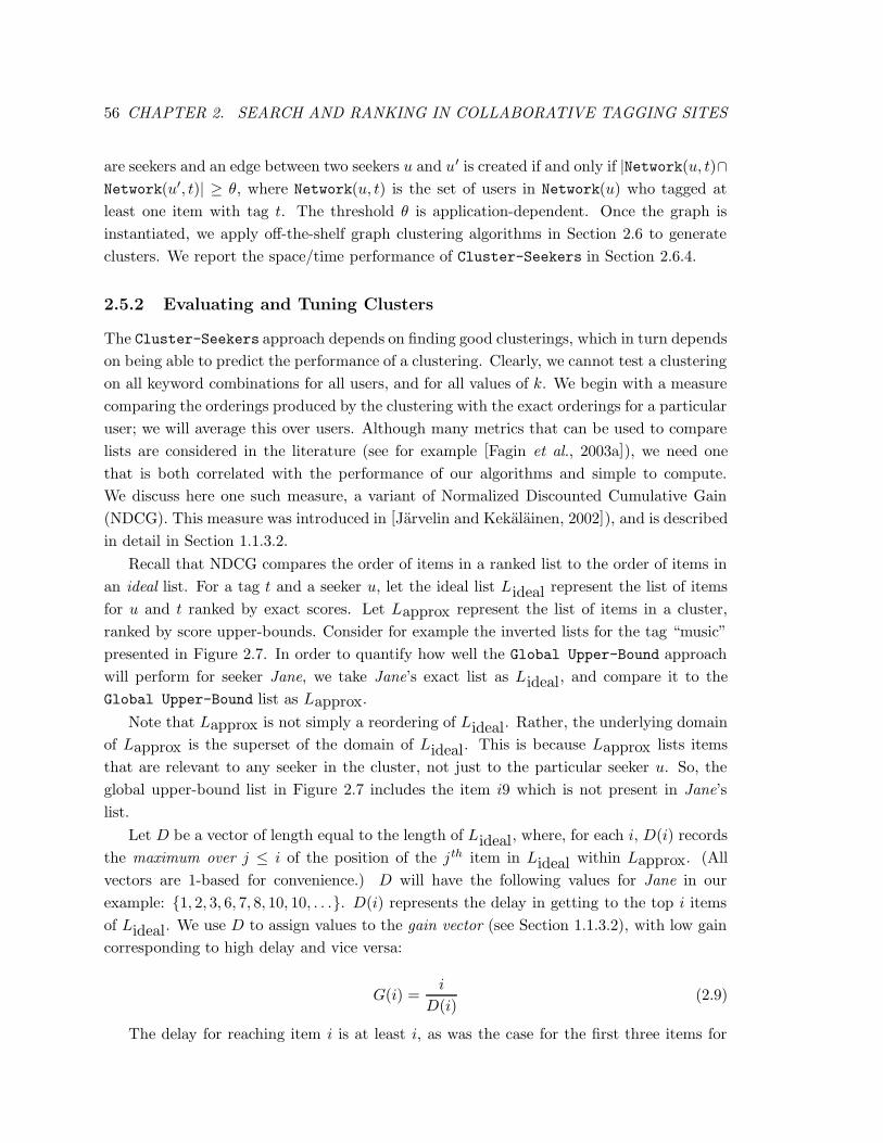
56 CHAPTER 2. SEARCH AND RANKING IN COLLABORATIVE TAGGING SITES
are seekers and an edge between two seekers u and u′ is created if and only if |Network(u, t)∩
Network(u′, t)| ≥ θ, where Network(u, t) is the set of users in Network(u) who tagged at
least one item with tag t. The threshold θ is application-dependent. Once the graph is
instantiated, we apply off-the-shelf graph clustering algorithms in Section 2.6 to generate
clusters. We report the space/time performance of Cluster-Seekers in Section 2.6.4.
2.5.2 Evaluating and Tuning Clusters
The Cluster-Seekers approach depends on finding good clusterings, which in turn depends
on being able to predict the performance of a clustering. Clearly, we cannot test a clustering
on all keyword combinations for all users, and for all values of k. We begin with a measure
comparing the orderings produced by the clustering with the exact orderings for a particular
user; we will average this over users. Although many metrics that can be used to compare
lists are considered in the literature (see for example [Fagin et al., 2003a]), we need one
that is both correlated with the performance of our algorithms and simple to compute.
We discuss here one such measure, a variant of Normalized Discounted Cumulative Gain
(NDCG). This measure was introduced in [Jarvelin and Kekalainen, 2002]), and is described
in detail in Section 1.1.3.2.
Recall that NDCG compares the order of items in a ranked list to the order of items in
an ideal list. For a tag t and a seeker u, let the ideal list Lideal represent the list of items
for u and t ranked by exact scores. Let Lapprox represent the list of items in a cluster,
ranked by score upper-bounds. Consider for example the inverted lists for the tag “music”
presented in Figure 2.7. In order to quantify how well the Global Upper-Bound approach
will perform for seeker Jane, we take Jane’s exact list as Lideal, and compare it to the
Global Upper-Bound list as Lapprox.
Note that Lapprox is not simply a reordering of Lideal. Rather, the underlying domain
of Lapprox is the superset of the domain of Lideal. This is because Lapprox lists items
that are relevant to any seeker in the cluster, not just to the particular seeker u. So, the
global upper-bound list in Figure 2.7 includes the item i9 which is not present in Jane’s
list.
Let D be a vector of length equal to the length of Lideal, where, for each i, D(i) records
the maximum over j ≤ i of the position of the j th item in Lideal within Lapprox. (All
vectors are 1-based for convenience.) D will have the following values for Jane in our
example: {1, 2, 3, 6, 7, 8, 10, 10, . . .}. D(i) represents the delay in getting to the top i items
of Lideal. We use D to assign values to the gain vector (see Section 1.1.3.2), with low gain
corresponding to high delay and vice versa:
G(i) =i
D(i)(2.9)
The delay for reaching item i is at least i, as was the case for the first three items for
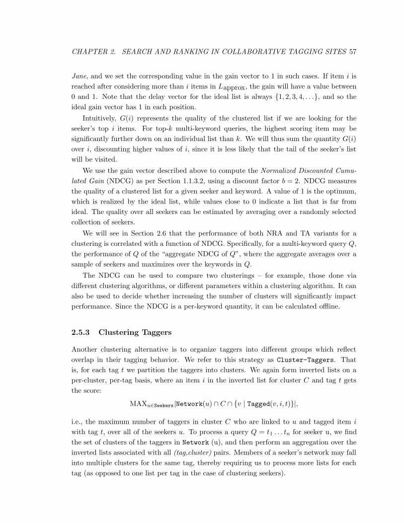
CHAPTER 2. SEARCH AND RANKING IN COLLABORATIVE TAGGING SITES 57
Jane, and we set the corresponding value in the gain vector to 1 in such cases. If item i is
reached after considering more than i items in Lapprox, the gain will have a value between
0 and 1. Note that the delay vector for the ideal list is always {1, 2, 3, 4, . . .}, and so the
ideal gain vector has 1 in each position.
Intuitively, G(i) represents the quality of the clustered list if we are looking for the
seeker’s top i items. For top-k multi-keyword queries, the highest scoring item may be
significantly further down on an individual list than k. We will thus sum the quantity G(i)
over i, discounting higher values of i, since it is less likely that the tail of the seeker’s list
will be visited.
We use the gain vector described above to compute the Normalized Discounted Cumu-
lated Gain (NDCG) as per Section 1.1.3.2, using a discount factor b = 2. NDCG measures
the quality of a clustered list for a given seeker and keyword. A value of 1 is the optimum,
which is realized by the ideal list, while values close to 0 indicate a list that is far from
ideal. The quality over all seekers can be estimated by averaging over a randomly selected
collection of seekers.
We will see in Section 2.6 that the performance of both NRA and TA variants for a
clustering is correlated with a function of NDCG. Specifically, for a multi-keyword query Q,
the performance of Q of the “aggregate NDCG of Q”, where the aggregate averages over a
sample of seekers and maximizes over the keywords in Q.
The NDCG can be used to compare two clusterings – for example, those done via
different clustering algorithms, or different parameters within a clustering algorithm. It can
also be used to decide whether increasing the number of clusters will significantly impact
performance. Since the NDCG is a per-keyword quantity, it can be calculated offline.
2.5.3 Clustering Taggers
Another clustering alternative is to organize taggers into different groups which reflect
overlap in their tagging behavior. We refer to this strategy as Cluster-Taggers. That
is, for each tag t we partition the taggers into clusters. We again form inverted lists on a
per-cluster, per-tag basis, where an item i in the inverted list for cluster C and tag t gets
the score:
MAXu∈Seekers|Network(u) ∩ C ∩ {v | Tagged(v, i, t)}|,
i.e., the maximum number of taggers in cluster C who are linked to u and tagged item i
with tag t, over all of the seekers u. To process a query Q = t1 . . . tn for seeker u, we find
the set of clusters of the taggers in Network (u), and then perform an aggregation over the
inverted lists associated with all (tag,cluster) pairs. Members of a seeker’s network may fall
into multiple clusters for the same tag, thereby requiring us to process more lists for each
tag (as opposed to one list per tag in the case of clustering seekers).
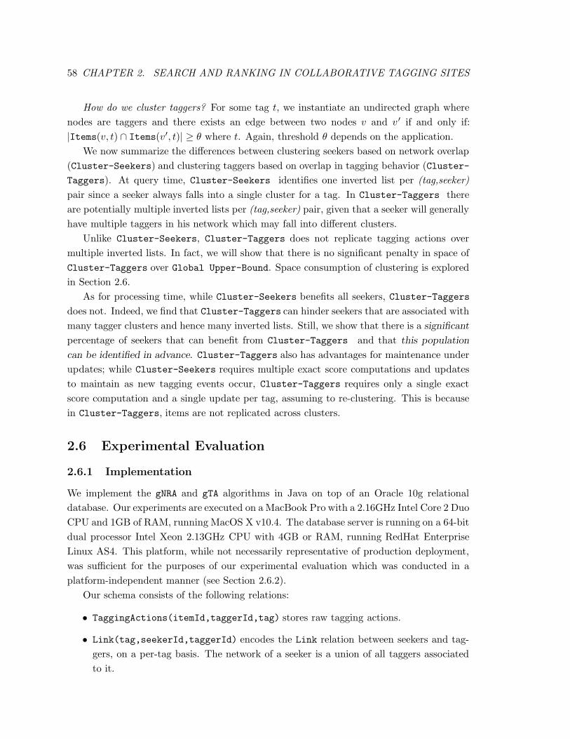
58 CHAPTER 2. SEARCH AND RANKING IN COLLABORATIVE TAGGING SITES
How do we cluster taggers? For some tag t, we instantiate an undirected graph where
nodes are taggers and there exists an edge between two nodes v and v ′ if and only if:
|Items(v, t) ∩ Items(v′, t)| ≥ θ where t. Again, threshold θ depends on the application.
We now summarize the differences between clustering seekers based on network overlap
(Cluster-Seekers) and clustering taggers based on overlap in tagging behavior (Cluster-
Taggers). At query time, Cluster-Seekers identifies one inverted list per (tag,seeker)
pair since a seeker always falls into a single cluster for a tag. In Cluster-Taggers there
are potentially multiple inverted lists per (tag,seeker) pair, given that a seeker will generally
have multiple taggers in his network which may fall into different clusters.
Unlike Cluster-Seekers, Cluster-Taggers does not replicate tagging actions over
multiple inverted lists. In fact, we will show that there is no significant penalty in space of
Cluster-Taggers over Global Upper-Bound. Space consumption of clustering is explored
in Section 2.6.
As for processing time, while Cluster-Seekers benefits all seekers, Cluster-Taggers
does not. Indeed, we find that Cluster-Taggers can hinder seekers that are associated with
many tagger clusters and hence many inverted lists. Still, we show that there is a significant
percentage of seekers that can benefit from Cluster-Taggers and that this population
can be identified in advance. Cluster-Taggers also has advantages for maintenance under
updates; while Cluster-Seekers requires multiple exact score computations and updates
to maintain as new tagging events occur, Cluster-Taggers requires only a single exact
score computation and a single update per tag, assuming to re-clustering. This is because
in Cluster-Taggers, items are not replicated across clusters.
2.6 Experimental Evaluation
2.6.1 Implementation
We implement the gNRA and gTA algorithms in Java on top of an Oracle 10g relational
database. Our experiments are executed on a MacBook Pro with a 2.16GHz Intel Core 2 Duo
CPU and 1GB of RAM, running MacOS X v10.4. The database server is running on a 64-bit
dual processor Intel Xeon 2.13GHz CPU with 4GB or RAM, running RedHat Enterprise
Linux AS4. This platform, while not necessarily representative of production deployment,
was sufficient for the purposes of our experimental evaluation which was conducted in a
platform-independent manner (see Section 2.6.2).
Our schema consists of the following relations:
• TaggingActions(itemId,taggerId,tag) stores raw tagging actions.
• Link(tag,seekerId,taggerId) encodes the Link relation between seekers and tag-
gers, on a per-tag basis. The network of a seeker is a union of all taggers associated
to it.
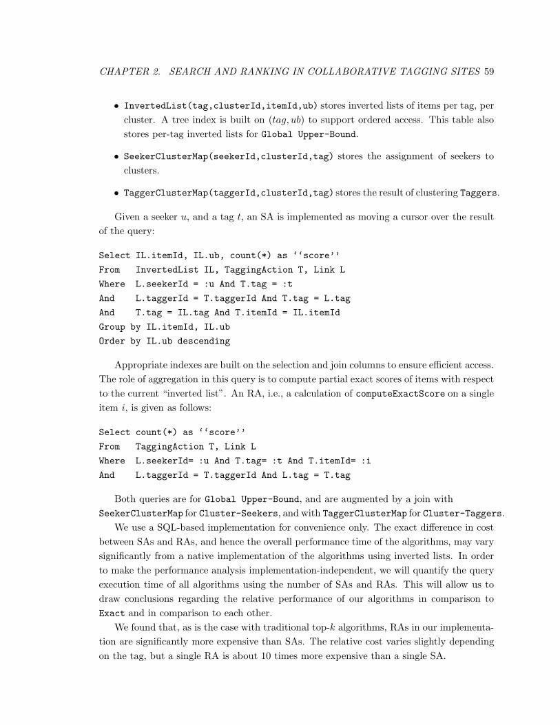
CHAPTER 2. SEARCH AND RANKING IN COLLABORATIVE TAGGING SITES 59
• InvertedList(tag,clusterId,itemId,ub) stores inverted lists of items per tag, per
cluster. A tree index is built on (tag, ub) to support ordered access. This table also
stores per-tag inverted lists for Global Upper-Bound.
• SeekerClusterMap(seekerId,clusterId,tag) stores the assignment of seekers to
clusters.
• TaggerClusterMap(taggerId,clusterId,tag) stores the result of clustering Taggers.
Given a seeker u, and a tag t, an SA is implemented as moving a cursor over the result
of the query:
Select IL.itemId, IL.ub, count(*) as ‘‘score’’
From InvertedList IL, TaggingAction T, Link L
Where L.seekerId = :u And T.tag = :t
And L.taggerId = T.taggerId And T.tag = L.tag
And T.tag = IL.tag And T.itemId = IL.itemId
Group by IL.itemId, IL.ub
Order by IL.ub descending
Appropriate indexes are built on the selection and join columns to ensure efficient access.
The role of aggregation in this query is to compute partial exact scores of items with respect
to the current “inverted list”. An RA, i.e., a calculation of computeExactScore on a single
item i, is given as follows:
Select count(*) as ‘‘score’’
From TaggingAction T, Link L
Where L.seekerId= :u And T.tag= :t And T.itemId= :i
And L.taggerId = T.taggerId And L.tag = T.tag
Both queries are for Global Upper-Bound, and are augmented by a join with
SeekerClusterMap for Cluster-Seekers, and with TaggerClusterMap for Cluster-Taggers.
We use a SQL-based implementation for convenience only. The exact difference in cost
between SAs and RAs, and hence the overall performance time of the algorithms, may vary
significantly from a native implementation of the algorithms using inverted lists. In order
to make the performance analysis implementation-independent, we will quantify the query
execution time of all algorithms using the number of SAs and RAs. This will allow us to
draw conclusions regarding the relative performance of our algorithms in comparison to
Exact and in comparison to each other.
We found that, as is the case with traditional top-k algorithms, RAs in our implementa-
tion are significantly more expensive than SAs. The relative cost varies slightly depending
on the tag, but a single RA is about 10 times more expensive than a single SA.
60 CHAPTER 2. SEARCH AND RANKING IN COLLABORATIVE TAGGING SITES
We use Graclus [Dhillon et al., 2007], an efficient clustering implementation over undi-
rected weighted graphs. Graclus provides two clustering methods. Ratio Association (ASC)
maximizes edge density within each cluster, while Normalized Cut (NCT) minimizes the
sum of weights on edges between clusters [Dhillon et al., 2007]. More formally, given two
sets of nodes Vi and Vj, we denote by links(Vi,Vj) the sum of edge weights between nodes
in Vi and nodes in Vj. We denote by degree(V) the sum of weights on edges incident on
the nodes in V. The objective of ASC is:
maximize
n∑
i=1
|links(Vi,Vi)|
|Vi|
The objective of NCT is:
minimize
n∑
i=1
|links(Vi,V \ Vi)|
degree(Vi)
2.6.2 Data and Evaluation Methods
We use a sample of Delicious for our experimental evaluation. Properties of the dataset
are described in Section 2.1.4, and we recall here that the dataset contains 116,177 distinct
users who tagged 175,691 distinct URLs using 903 distinct tags, for a total of 2,322,458
tagging actions.
We choose 4 tags (software, programming, tutorial, and reference) from the 20 most
popular. Popularity of a tag is measured by the total number of tagging actions involving
it: the most popular tag has been used about 100,000 times, while the 20th most popular
was used about 34,000 times. We evaluate the performance of our methods over 6 queries
of varying lengths, to which we refer by the first letters of each tag. The queries were SP
for software programming, TR for tutorial reference, PR for programming reference, SPT
for software programming tutorial, SPR for software programming reference, and SPTR
for software programming tutorial reference. We chose these four tags because they are
thematically related and may be meaningfully combined in a query.
As we described in Section 2.1.2, Delicious has an explicit notion of friendship. How-
ever, users may have various semantics for it. Since we are interested in networks that
reflect affinities in item preference, in our experiments we use a network derived from the
tagging data via common interest. This choice is supported by our experimental results
in Section 2.2, where we find that a common-interest network reflects the user’s interests
more closely than does the explicit friendship network. In the network that was used for
the purposes of our experimental evaluation, there is a link between a seeker and a tagger
if they tagged at least two items in common with the same tag.
Due to the choice of the network, only seekers who are also taggers are included in
the experimental evaluation. However, as mentioned in Section 2.3.2, the techniques of
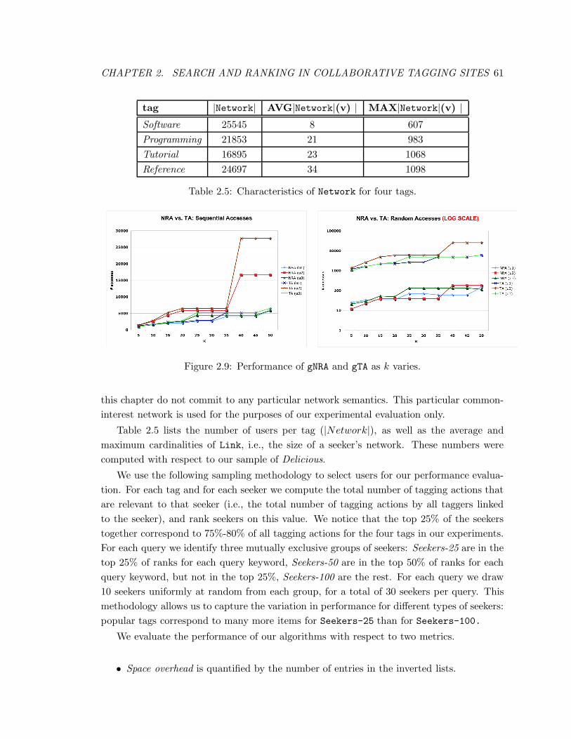
CHAPTER 2. SEARCH AND RANKING IN COLLABORATIVE TAGGING SITES 61
tag |Network| AVG|Network|(v) | MAX|Network|(v) |
Software 25545 8 607
Programming 21853 21 983
Tutorial 16895 23 1068
Reference 24697 34 1098
Table 2.5: Characteristics of Network for four tags.
Figure 2.9: Performance of gNRA and gTA as k varies.
this chapter do not commit to any particular network semantics. This particular common-
interest network is used for the purposes of our experimental evaluation only.
Table 2.5 lists the number of users per tag (|Network|), as well as the average and
maximum cardinalities of Link, i.e., the size of a seeker’s network. These numbers were
computed with respect to our sample of Delicious.
We use the following sampling methodology to select users for our performance evalua-
tion. For each tag and for each seeker we compute the total number of tagging actions that
are relevant to that seeker (i.e., the total number of tagging actions by all taggers linked
to the seeker), and rank seekers on this value. We notice that the top 25% of the seekers
together correspond to 75%-80% of all tagging actions for the four tags in our experiments.
For each query we identify three mutually exclusive groups of seekers: Seekers-25 are in the
top 25% of ranks for each query keyword, Seekers-50 are in the top 50% of ranks for each
query keyword, but not in the top 25%, Seekers-100 are the rest. For each query we draw
10 seekers uniformly at random from each group, for a total of 30 seekers per query. This
methodology allows us to capture the variation in performance for different types of seekers:
popular tags correspond to many more items for Seekers-25 than for Seekers-100.
We evaluate the performance of our algorithms with respect to two metrics.
• Space overhead is quantified by the number of entries in the inverted lists.
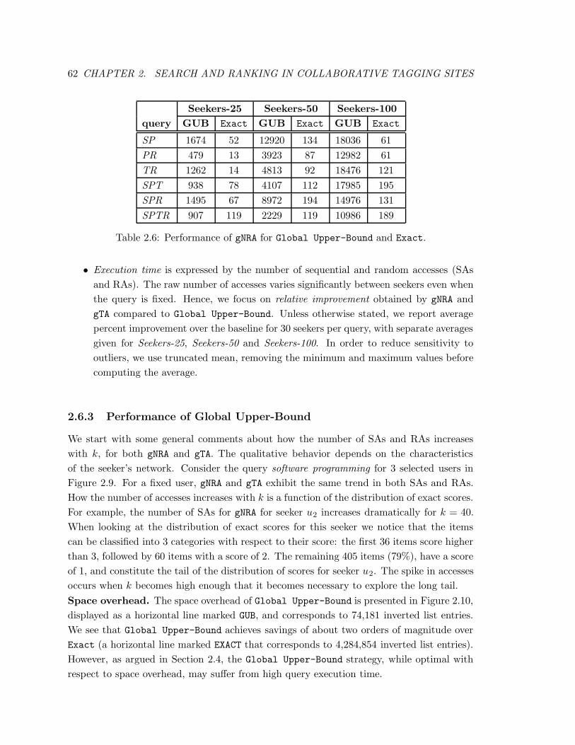
62 CHAPTER 2. SEARCH AND RANKING IN COLLABORATIVE TAGGING SITES
Seekers-25 Seekers-50 Seekers-100
query GUB Exact GUB Exact GUB Exact
SP 1674 52 12920 134 18036 61
PR 479 13 3923 87 12982 61
TR 1262 14 4813 92 18476 121
SPT 938 78 4107 112 17985 195
SPR 1495 67 8972 194 14976 131
SPTR 907 119 2229 119 10986 189
Table 2.6: Performance of gNRA for Global Upper-Bound and Exact.
• Execution time is expressed by the number of sequential and random accesses (SAs
and RAs). The raw number of accesses varies significantly between seekers even when
the query is fixed. Hence, we focus on relative improvement obtained by gNRA and
gTA compared to Global Upper-Bound. Unless otherwise stated, we report average
percent improvement over the baseline for 30 seekers per query, with separate averages
given for Seekers-25, Seekers-50 and Seekers-100. In order to reduce sensitivity to
outliers, we use truncated mean, removing the minimum and maximum values before
computing the average.
2.6.3 Performance of Global Upper-Bound
We start with some general comments about how the number of SAs and RAs increases
with k, for both gNRA and gTA. The qualitative behavior depends on the characteristics
of the seeker’s network. Consider the query software programming for 3 selected users in
Figure 2.9. For a fixed user, gNRA and gTA exhibit the same trend in both SAs and RAs.
How the number of accesses increases with k is a function of the distribution of exact scores.
For example, the number of SAs for gNRA for seeker u2 increases dramatically for k = 40.
When looking at the distribution of exact scores for this seeker we notice that the items
can be classified into 3 categories with respect to their score: the first 36 items score higher
than 3, followed by 60 items with a score of 2. The remaining 405 items (79%), have a score
of 1, and constitute the tail of the distribution of scores for seeker u2. The spike in accesses
occurs when k becomes high enough that it becomes necessary to explore the long tail.
Space overhead. The space overhead of Global Upper-Bound is presented in Figure 2.10,
displayed as a horizontal line marked GUB, and corresponds to 74,181 inverted list entries.
We see that Global Upper-Bound achieves savings of about two orders of magnitude over
Exact (a horizontal line marked EXACT that corresponds to 4,284,854 inverted list entries).
However, as argued in Section 2.4, the Global Upper-Bound strategy, while optimal with
respect to space overhead, may suffer from high query execution time.
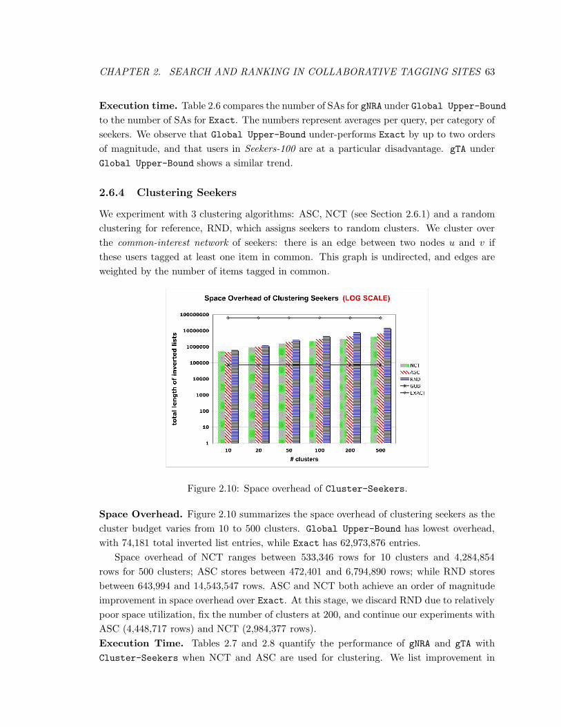
CHAPTER 2. SEARCH AND RANKING IN COLLABORATIVE TAGGING SITES 63
Execution time. Table 2.6 compares the number of SAs for gNRA under Global Upper-Bound
to the number of SAs for Exact. The numbers represent averages per query, per category of
seekers. We observe that Global Upper-Bound under-performs Exact by up to two orders
of magnitude, and that users in Seekers-100 are at a particular disadvantage. gTA under
Global Upper-Bound shows a similar trend.
2.6.4 Clustering Seekers
We experiment with 3 clustering algorithms: ASC, NCT (see Section 2.6.1) and a random
clustering for reference, RND, which assigns seekers to random clusters. We cluster over
the common-interest network of seekers: there is an edge between two nodes u and v if
these users tagged at least one item in common. This graph is undirected, and edges are
weighted by the number of items tagged in common.
Figure 2.10: Space overhead of Cluster-Seekers.
Space Overhead. Figure 2.10 summarizes the space overhead of clustering seekers as the
cluster budget varies from 10 to 500 clusters. Global Upper-Bound has lowest overhead,
with 74,181 total inverted list entries, while Exact has 62,973,876 entries.
Space overhead of NCT ranges between 533,346 rows for 10 clusters and 4,284,854
rows for 500 clusters; ASC stores between 472,401 and 6,794,890 rows; while RND stores
between 643,994 and 14,543,547 rows. ASC and NCT both achieve an order of magnitude
improvement in space overhead over Exact. At this stage, we discard RND due to relatively
poor space utilization, fix the number of clusters at 200, and continue our experiments with
ASC (4,448,717 rows) and NCT (2,984,377 rows).
Execution Time. Tables 2.7 and 2.8 quantify the performance of gNRA and gTA with
Cluster-Seekers when NCT and ASC are used for clustering. We list improvement in
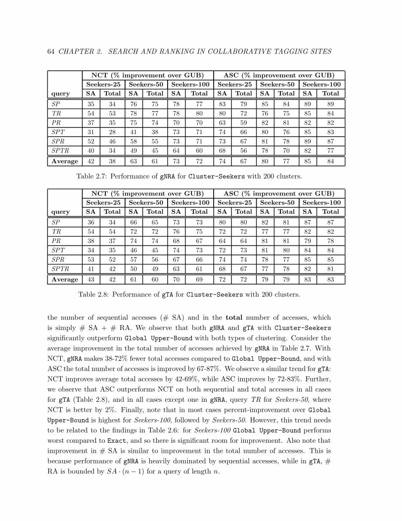
64 CHAPTER 2. SEARCH AND RANKING IN COLLABORATIVE TAGGING SITES
NCT (% improvement over GUB) ASC (% improvement over GUB)
Seekers-25 Seekers-50 Seekers-100 Seekers-25 Seekers-50 Seekers-100
query SA Total SA Total SA Total SA Total SA Total SA Total
SP 35 34 76 75 78 77 83 79 85 84 89 89
TR 54 53 78 77 78 80 80 72 76 75 85 84
PR 37 35 75 74 70 70 63 59 82 81 82 82
SPT 31 28 41 38 73 71 74 66 80 76 85 83
SPR 52 46 58 55 73 71 73 67 81 78 89 87
SPTR 40 34 49 45 64 60 68 56 78 70 82 77
Average 42 38 63 61 73 72 74 67 80 77 85 84
Table 2.7: Performance of gNRA for Cluster-Seekers with 200 clusters.
NCT (% improvement over GUB) ASC (% improvement over GUB)
Seekers-25 Seekers-50 Seekers-100 Seekers-25 Seekers-50 Seekers-100
query SA Total SA Total SA Total SA Total SA Total SA Total
SP 36 34 66 65 73 73 80 80 82 81 87 87
TR 54 54 72 72 76 75 72 72 77 77 82 82
PR 38 37 74 74 68 67 64 64 81 81 79 78
SPT 34 35 46 45 74 73 72 73 81 80 84 84
SPR 53 52 57 56 67 66 74 74 78 77 85 85
SPTR 41 42 50 49 63 61 68 67 77 78 82 81
Average 43 42 61 60 70 69 72 72 79 79 83 83
Table 2.8: Performance of gTA for Cluster-Seekers with 200 clusters.
the number of sequential accesses (# SA) and in the total number of accesses, which
is simply # SA + # RA. We observe that both gNRA and gTA with Cluster-Seekers
significantly outperform Global Upper-Bound with both types of clustering. Consider the
average improvement in the total number of accesses achieved by gNRA in Table 2.7. With
NCT, gNRA makes 38-72% fewer total accesses compared to Global Upper-Bound, and with
ASC the total number of accesses is improved by 67-87%. We observe a similar trend for gTA:
NCT improves average total accesses by 42-69%, while ASC improves by 72-83%. Further,
we observe that ASC outperforms NCT on both sequential and total accesses in all cases
for gTA (Table 2.8), and in all cases except one in gNRA, query TR for Seekers-50, where
NCT is better by 2%. Finally, note that in most cases percent-improvement over Global
Upper-Bound is highest for Seekers-100, followed by Seekers-50. However, this trend needs
to be related to the findings in Table 2.6: for Seekers-100 Global Upper-Bound performs
worst compared to Exact, and so there is significant room for improvement. Also note that
improvement in # SA is similar to improvement in the total number of accesses. This is
because performance of gNRA is heavily dominated by sequential accesses, while in gTA, #
RA is bounded by SA · (n− 1) for a query of length n.
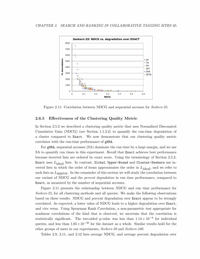
CHAPTER 2. SEARCH AND RANKING IN COLLABORATIVE TAGGING SITES 65
Seekers-25: NDCG vs. degradation over EXACT
0
1000
2000
3000
4000
5000
6000
7000
8000
0 0.1 0.2 0.3 0.4 0.5 0.6
NDCG
% d
eg
rad
ati
on SP
TR
PR
SPT
SPR
SPTR
Figure 2.11: Correlation between NDCG and sequential accesses for Seekers-25.
2.6.5 Effectiveness of the Clustering Quality Metric
In Section 2.5.2 we described a clustering quality metric that uses Normalized Discounted
Cumulative Gain (NDCG) (see Section 1.1.3.2) to quantify the run-time degradation of
a cluster compared to Exact. We now demonstrate that our clustering quality metric
correlates with the run-time performance of gNRA.
For gNRA, sequential accesses (SA) dominate the run time by a large margin, and we use
SA to quantify run times in this experiment. Recall that Exact achieves best performance
because inverted lists are ordered by exact score. Using the terminology of Section 2.5.2,
Exact uses Lideal lists. In contrast, Global Upper-Bound and Cluster-Seekers use in-
verted lists in which the order of items approximates the order in Lideal, and we refer to
such lists as Lapprox. In the remainder of this section we will study the correlation between
our variant of NDCG and the percent degradation in run time performance, compared to
Exact, as measured by the number of sequential accesses.
Figure 2.11 presents the relationship between NDCG and run time performance for
Seekers-25, for all clustering methods and all queries. We make the following observations
based on these results. NDCG and percent degradation over Exact appear to be strongly
correlated. As expected, a lower value of NDCG leads to a higher degradation over Exact,
and vice versa. Using Spearman Rank Correlation, a non-parametric test appropriate for
nonlinear correlations of the kind that is observed, we ascertain that the correlation is
statistically significant. The two-sided p-value was less than 1.14 ∗ 10−6 for individual
queries, and less than 1.65 ∗ 10−39 for the dataset as a whole. Similar results hold for the
other groups of users in our experiments, Seekers-50 and Seekers-100.
Tables 2.9, 2.11, and 2.12 lists average NDCG, and average percent degradation over
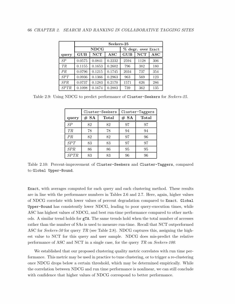
66 CHAPTER 2. SEARCH AND RANKING IN COLLABORATIVE TAGGING SITES
Seekers-25
NDCG % degr. over Exact
query GUB NCT ASC GUB NCT ASC
SP 0.0575 0.0841 0.2232 2594 1128 306
TR 0.1155 0.1653 0.2602 796 382 180
PR 0.0796 0.1215 0.1745 2034 737 354
SPT 0.0936 0.1366 0.2963 963 569 123
SPR 0.0737 0.1283 0.2170 1571 626 286
SPTR 0.1098 0.1674 0.2883 739 362 135
Table 2.9: Using NDCG to predict performance of Cluster-Seekers for Seekers-25.
Cluster-Seekers Cluster-Taggers
query # SA Total # SA Total
SP 82 82 97 97
TR 78 78 94 94
PR 82 82 97 96
SPT 83 83 97 97
SPR 86 86 95 95
SPTR 83 83 96 96
Table 2.10: Percent-improvement of Cluster-Seekers and Cluster-Taggers, compared
to Global Upper-Bound.
Exact, with averages computed for each query and each clustering method. These results
are in line with the performance numbers in Tables 2.6 and 2.7. Here, again, higher values
of NDCG correlate with lower values of percent degradation compared to Exact. Global
Upper-Bound has consistently lower NDCG, leading to poor query-execution times, while
ASC has highest values of NDCG, and best run-time performance compared to other meth-
ods. A similar trend holds for gTA. The same trends hold when the total number of accesses
rather than the number of SAs is used to measure run-time. Recall that NCT outperformed
ASC for Seekers-50 for query TR (see Table 2.8). NDCG captures this, assigning the high-
est value to NCT for this query and user sample. NDCG does mis-predict the relative
performance of ASC and NCT in a single case, for the query TR on Seekers-100.
We established that our proposed clustering quality metric correlates with run time per-
formance. This metric may be used in practice to tune clustering, or to trigger a re-clustering
once NDCG drops below a certain threshold, which may be determined empirically. While
the correlation between NDCG and run time performance is nonlinear, we can still conclude
with confidence that higher values of NDCG correspond to better performance.
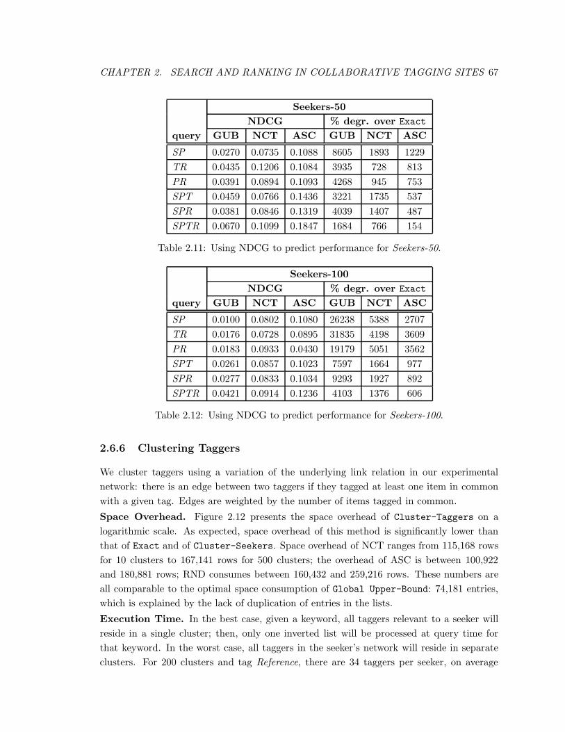
CHAPTER 2. SEARCH AND RANKING IN COLLABORATIVE TAGGING SITES 67
Seekers-50
NDCG % degr. over Exact
query GUB NCT ASC GUB NCT ASC
SP 0.0270 0.0735 0.1088 8605 1893 1229
TR 0.0435 0.1206 0.1084 3935 728 813
PR 0.0391 0.0894 0.1093 4268 945 753
SPT 0.0459 0.0766 0.1436 3221 1735 537
SPR 0.0381 0.0846 0.1319 4039 1407 487
SPTR 0.0670 0.1099 0.1847 1684 766 154
Table 2.11: Using NDCG to predict performance for Seekers-50.
Seekers-100
NDCG % degr. over Exact
query GUB NCT ASC GUB NCT ASC
SP 0.0100 0.0802 0.1080 26238 5388 2707
TR 0.0176 0.0728 0.0895 31835 4198 3609
PR 0.0183 0.0933 0.0430 19179 5051 3562
SPT 0.0261 0.0857 0.1023 7597 1664 977
SPR 0.0277 0.0833 0.1034 9293 1927 892
SPTR 0.0421 0.0914 0.1236 4103 1376 606
Table 2.12: Using NDCG to predict performance for Seekers-100.
2.6.6 Clustering Taggers
We cluster taggers using a variation of the underlying link relation in our experimental
network: there is an edge between two taggers if they tagged at least one item in common
with a given tag. Edges are weighted by the number of items tagged in common.
Space Overhead. Figure 2.12 presents the space overhead of Cluster-Taggers on a
logarithmic scale. As expected, space overhead of this method is significantly lower than
that of Exact and of Cluster-Seekers. Space overhead of NCT ranges from 115,168 rows
for 10 clusters to 167,141 rows for 500 clusters; the overhead of ASC is between 100,922
and 180,881 rows; RND consumes between 160,432 and 259,216 rows. These numbers are
all comparable to the optimal space consumption of Global Upper-Bound: 74,181 entries,
which is explained by the lack of duplication of entries in the lists.
Execution Time. In the best case, given a keyword, all taggers relevant to a seeker will
reside in a single cluster; then, only one inverted list will be processed at query time for
that keyword. In the worst case, all taggers in the seeker’s network will reside in separate
clusters. For 200 clusters and tag Reference, there are 34 taggers per seeker, on average
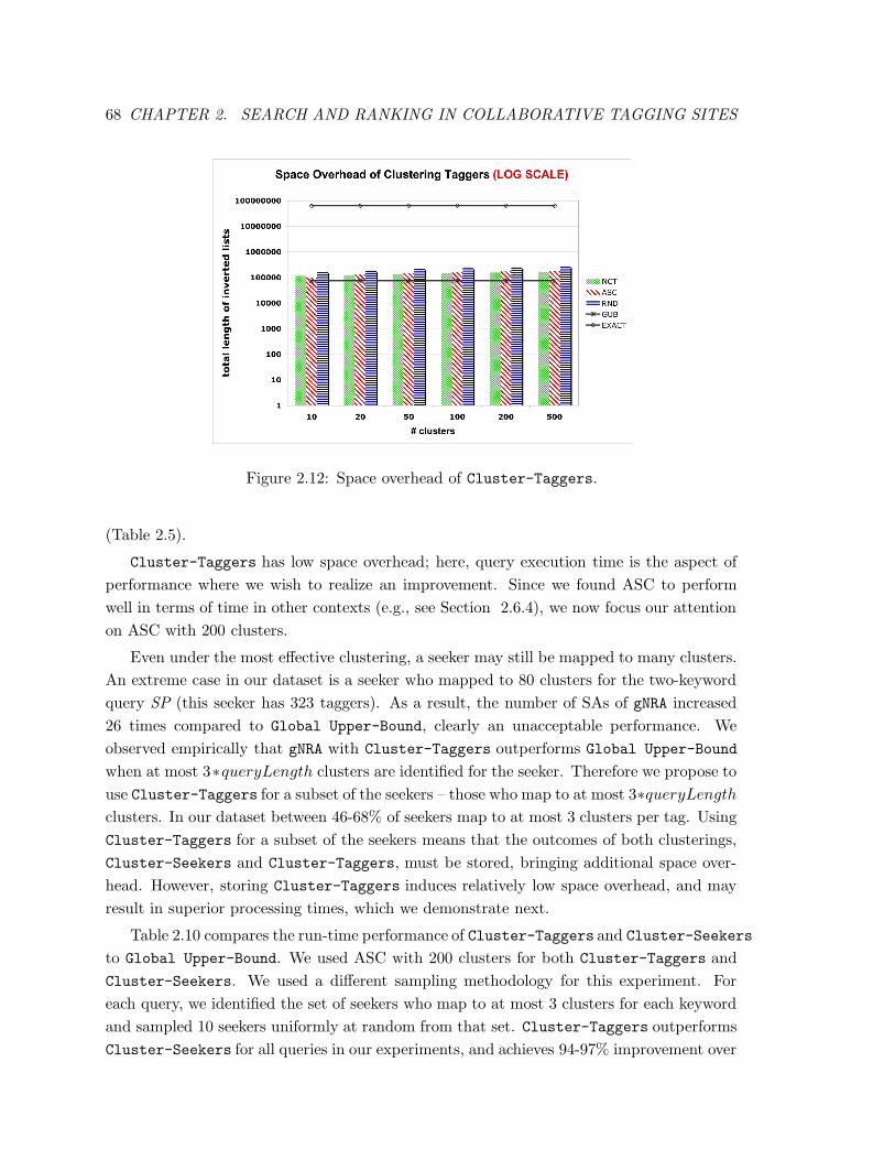
68 CHAPTER 2. SEARCH AND RANKING IN COLLABORATIVE TAGGING SITES
Figure 2.12: Space overhead of Cluster-Taggers.
(Table 2.5).
Cluster-Taggers has low space overhead; here, query execution time is the aspect of
performance where we wish to realize an improvement. Since we found ASC to perform
well in terms of time in other contexts (e.g., see Section 2.6.4), we now focus our attention
on ASC with 200 clusters.
Even under the most effective clustering, a seeker may still be mapped to many clusters.
An extreme case in our dataset is a seeker who mapped to 80 clusters for the two-keyword
query SP (this seeker has 323 taggers). As a result, the number of SAs of gNRA increased
26 times compared to Global Upper-Bound, clearly an unacceptable performance. We
observed empirically that gNRA with Cluster-Taggers outperforms Global Upper-Bound
when at most 3∗queryLength clusters are identified for the seeker. Therefore we propose to
use Cluster-Taggers for a subset of the seekers – those who map to at most 3∗queryLength
clusters. In our dataset between 46-68% of seekers map to at most 3 clusters per tag. Using
Cluster-Taggers for a subset of the seekers means that the outcomes of both clusterings,
Cluster-Seekers and Cluster-Taggers, must be stored, bringing additional space over-
head. However, storing Cluster-Taggers induces relatively low space overhead, and may
result in superior processing times, which we demonstrate next.
Table 2.10 compares the run-time performance of Cluster-Taggers and Cluster-Seekers
to Global Upper-Bound. We used ASC with 200 clusters for both Cluster-Taggers and
Cluster-Seekers. We used a different sampling methodology for this experiment. For
each query, we identified the set of seekers who map to at most 3 clusters for each keyword
and sampled 10 seekers uniformly at random from that set. Cluster-Taggers outperforms
Cluster-Seekers for all queries in our experiments, and achieves 94-97% improvement over
CHAPTER 2. SEARCH AND RANKING IN COLLABORATIVE TAGGING SITES 69
Global Upper-Bound for this class of seekers. This is because tagging actions of a particular
tagger are not replicated across clusters in the Cluster-Taggers clustering scheme. As a re-
sult, per-cluster inverted lists in Cluster-Taggers are typically shorter, and upper-bounds
are much closer to exact scores of the items.
2.7 Related Work
Top-k Processing: Top-k algorithms aim to reduce the amount of processing required
to compute the top-ranked answers, and have been used in the relational [Carey and
Kossmann, 1997], XML [Marian et al., 2005], and other settings. The core ideas of these
algorithms are overviewed in [Fagin et al., 2003c; Fagin, 2002]. A common assumption is
that scores are used to maintain dynamic thresholds during query processing, in order to
efficiently prune low-scoring answers.
Even in work where the underlying query model is distributed [Michel et al., 2005], or
where the aggregation computation is expensive [Hwang and Chang, 2007], this assump-
tion of pre-computation remains in place. In our work, we extend Fagin-style algorithms
to process score upper-bounds – since pre-computed scores for each individual seeker are
too expensive to store (given that they depend on a seeker’s network) – and we explore
clustering as a way to refine upper-bounds and reduce the size of the inverted lists.
Clustering: Graph clustering algorithms are plentiful and generally work on graphs with
(possibly weighted) edges. Most of the work on clustering has focused on minimizing cluster-
ing time and considering additional constraints such as producing same-size clusters. In our
experiments, we use Graclus, an open-source graph clustering software that is based on two
variants of the popular k-means algorithms: normalized cut and ratio association [Dhillon
et al., 2007].
Socially Influenced Search: Although the potential of using social ties to improve
search has been recognized for some time, this is still subject of ongoing work. Current
research has focused on judging the impact of various notions of user affinity and socially-
influenced scoring functions on search quality [Mislove et al., 2006; Zhou et al., 2008;
Li et al., 2008]. In contrast, our work develops indexing and query evaluation methods
which apply to a wide class of scoring functions and networks.
User Experience in Collaborative Tagging Sites: The idea of motivating partici-
pation by displaying the value of contribution is characteristic of collaborative reviewing
sites [Rashid et al., 2006] but has received little attention in the study of collaborative tag-
ging sites. Impact of reviews has been studied extensively in the e-commerce arena, and it
has been shown that reviews impact sales [Chen et al., 2007; Chevalier and Mayzlin, 2006;
70 CHAPTER 2. SEARCH AND RANKING IN COLLABORATIVE TAGGING SITES
Ghose and Ipeirotis, 2006]. Most of the current scientific literature dealing with user-
contributed reviews concerns text analysis to distill reviews [Popescu and Etzioni, 2005],
sentiment detection [Pang and Lee, 2004; Pang and Lee, 2005], and the impact of reviews
on product sales [Bickart and Schindler, 2001; Ghose and Ipeirotis, 2007; Kim et al., 2006;
Lio et al., 2007]. In contrast, very little has been done to extract value in collaborative
tagging systems and provide participation incentives to users.
Deriving Semantics from Social Tagging: Wu et al. [Wu et al., 2006b] present a
probabilistic generative model that uses tagging to obtain the emergent semantics in so-
cial annotations. The authors study the relationship between resources, tags, and users by
means of co-occurence analysis, and map these elements to a multi-dimensional conceptual
space, where each dimension represents a category of knowledge. The authors demonstrate
how these distributions may be learned and subsequently used to derive tag ambiguity in-
formation. They go on to show how their probabilistic model may be used for semantic
search and discovery in social tagging sites like Delicious.
Collaborative Filtering: Collaborative Filtering (CF) is a popular method which is based
on using machine learning to derive and compare user profiles in order to determine overlap
of interest between users. A user profile is built from explicit or implicit data. The system
can explicitly ask users to rate an item on a numerical scale, or to rank a collection of
items from most to least favorite. The system can also record items that a user browsed or
purchased, and analyze item viewing times. CF compares data collected from the user to
similar data collected from others and calculates a list of recommended items for the user.
Several methods have been developed to address data sparsity. Most of them (item-based
and user-based) rely on statistical approximation [Bell et al., 2007; Park and Pennock,
2007].
Our method differs from CF in that we express a user’s interest qualitatively rather
than quantitatively, using tags and derived ties. In [Agichtein et al., 2006], it is shown
that ranking in Web search can be improved by incorporating user behavior. Similarly,
we show that incorporating tagging behavior improves ranking in producing hotlists. This
motivates the need to better understand the principles behind designing a recommender
tagging system, as was briefly discussed in [Golder and Huberman, 2006]. According to
a study of del.icio.us tagging practices described in [Kipp and Campbell, 2006], tagging
exhibits self-organizing patterns. In our work we explore how users can be classified into
groups based on their tagging behavior, and how such groups can be used to improve the
quality of recommended hotlists.

CHAPTER 2. SEARCH AND RANKING IN COLLABORATIVE TAGGING SITES 71
2.8 Conclusion
In this chapter we presented the types of semantic context that exist in collaborative tagging
sites, and showed how such context can be used to improve the quality of search and ranking.
We first explored how a user’s social behavior and tagging can be used to produce high-
quality hotlists. We then presented network-aware search, a first attempt to incorporate
social behavior into searching in collaborative tagging sites.
We defined a model in which item scores are based on popularity among a network
of related users, and formalized top-k processing in this context. We demonstrated how
traditional algorithms can be extended to compute the best answers in a network-aware
manner, and proposed clustering seekers and taggers as a way to balance between processing
time and space consumption.
Incorporating a user’s social context into search and ranking is central to supporting
personalized social consumption of information, and provides a valuable participation in-
centive in collaborative tagging sites and beyond. A user who is able to access relevant
information with ease in a social manner is likely to engage the system more actively, both
by contributing content and creating social ties, and by consuming content provided by
other users. Socially-influenced search uses the semantics of social connections, and has as
one of its goals information discovery and the formation of knowledge. In the following chap-
ter we will consider a different but related aspect of information discovery. There, search
and ranking are likewise aimed at information discovery, and are based on the semantic
knowledge in domain ontologies.

72 CHAPTER 2. SEARCH AND RANKING IN COLLABORATIVE TAGGING SITES
CHAPTER 3. SEMANTIC RANKING FOR LIFE SCIENCES PUBLICATIONS 73
Chapter 3
Semantic Ranking for Life Sciences
Publications
This chapter is based on joint work with Kenneth A. Ross and William Mee and will appear
in [Stoyanovich et al., 2010].
3.1 Introduction
Many scientific domains, most notably the domain of life sciences, are experiencing unprece-
dented growth. The recent complete sequencing of the Human Genome, and the tremendous
advances in experimental technology are rapidly bringing about new scientific knowledge.
The ever-increasing amount of data and semantic knowledge in life sciences requires the
development of new semantically rich data management techniques that facilitate scientific
research and collaboration.
Literature search is a central task in scientific research. In their search users may pursue
different goals. For example, a user may need an overview of a broad area of research
that is outside his main field of expertise, or he may need to find new publications in an
area in which he is an expert. PubMed (www.pubmed.gov) is perhaps the most significant
bibliographic source in the domain of life sciences, with over 18 million articles at the time
of this writing. Indexed articles go back to 1865, and the number of articles grows daily, and
increases steadily from year to year. PubMed articles are manually annotated with terms
from the Medical Subject Headings (MeSH) controlled vocabulary. MeSH organizes term
descriptors into a hierarchical structure, allowing searching at various levels of specificity.
The 2008 version of MeSH contains 24,767 term descriptors that refer to general concepts
like Anatomy and Mental Disorders, as well as to specific concepts like Antiphospholipid
Syndrome and Cholesterol.
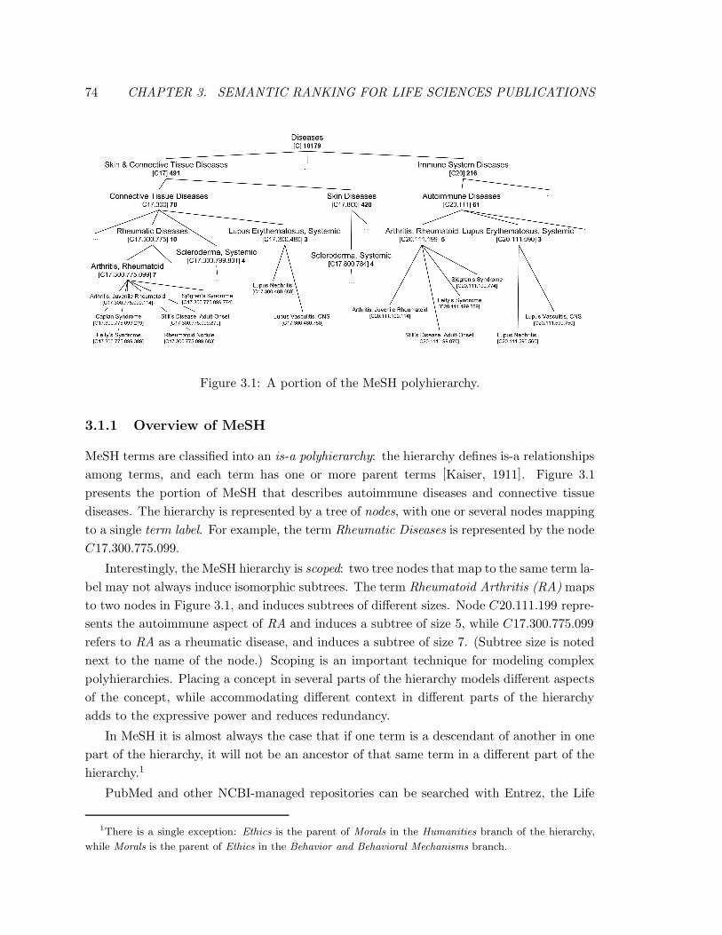
74 CHAPTER 3. SEMANTIC RANKING FOR LIFE SCIENCES PUBLICATIONS
Figure 3.1: A portion of the MeSH polyhierarchy.
3.1.1 Overview of MeSH
MeSH terms are classified into an is-a polyhierarchy: the hierarchy defines is-a relationships
among terms, and each term has one or more parent terms [Kaiser, 1911]. Figure 3.1
presents the portion of MeSH that describes autoimmune diseases and connective tissue
diseases. The hierarchy is represented by a tree of nodes, with one or several nodes mapping
to a single term label. For example, the term Rheumatic Diseases is represented by the node
C17.300.775.099.
Interestingly, the MeSH hierarchy is scoped: two tree nodes that map to the same term la-
bel may not always induce isomorphic subtrees. The term Rheumatoid Arthritis (RA) maps
to two nodes in Figure 3.1, and induces subtrees of different sizes. Node C20.111.199 repre-
sents the autoimmune aspect of RA and induces a subtree of size 5, while C17.300.775.099
refers to RA as a rheumatic disease, and induces a subtree of size 7. (Subtree size is noted
next to the name of the node.) Scoping is an important technique for modeling complex
polyhierarchies. Placing a concept in several parts of the hierarchy models different aspects
of the concept, while accommodating different context in different parts of the hierarchy
adds to the expressive power and reduces redundancy.
In MeSH it is almost always the case that if one term is a descendant of another in one
part of the hierarchy, it will not be an ancestor of that same term in a different part of the
hierarchy.1
PubMed and other NCBI-managed repositories can be searched with Entrez, the Life
1There is a single exception: Ethics is the parent of Morals in the Humanities branch of the hierarchy,
while Morals is the parent of Ethics in the Behavior and Behavioral Mechanisms branch.
CHAPTER 3. SEMANTIC RANKING FOR LIFE SCIENCES PUBLICATIONS 75
Sciences Search Engine2. Entrez implements sophisticated query processing, allowing the
user to specify conjunctive or disjunctive boolean semantics for the search query, and to
relate the search terms to one or several parts of the document: title, MeSH annotations,
text of the document, etc. In order to improve recall, Entrez automatically expands query
terms that are related to MeSH annotations with synonymous or near-synonymous terms.
For example, the simple query mosquito will be transformed by Entrez to “culicidae”[MeSH
Terms] OR “culicidae”[All Fields] OR “mosquito”[All Fields]. Entrez also expands the
query with descendants of any MeSH terms. For example, the query “blood cells”[MeSH
Terms] will match articles that are annotated with “blood cells” or with “erythrocytes”,
“leukocytes”, “hemocytes”, etc.
3.1.2 Challenges of Bibliographic Search
The need to improve recall differentiates bibliographic search from general web search.
In web search it is often assumed that many documents equivalently satisfy the user’s
information need, and so high recall is less important than high precision among the top-
ranked documents. Conversely, in bibliographic search the assumption (or at least the hope)
is that every scientific article contributes something novel to the state of the art, and so
no two documents are interchangeable when it comes to satisfying the user’s information
need. In this scenario the boolean retrieval model, such as that used by Entrez, guarantees
perfect recall and is the right choice.
However, there is an important common characteristic of bibliographic and general
web search: many queries return hundreds, or even thousands, of relevant results. Query
expansion techniques that maximize recall exacerbate this problem by producing yet more
results. For example, the fairly specific query Antiphospholipid Antibodies AND Thrombosis,
which looks for information about a particular clinical manifestation of antiphospholipid
syndrome, returned 2455 matches using the default query translation in January 2009. A
more general query that looks for articles about connective tissue diseases that are also
autoimmune returns close to 120,000 results.
Because so many results are returned per query, the system needs to help the user
explore the result set. Entrez currently allows the results to be sorted by several metadata
fields: publication date, first author, last author, journal, and title. This may help the
user look up an article with which he is already familiar (i.e., knows some of the associated
metadata), but does not support true information discovery.
A useful and well-known way to order results in web information retrieval is by query
relevance. Retrieval models such as the Vector Space Model [Baeza-Yates and Ribeiro-Neto,
1999] have the query relevance metric built in, while the boolean retrieval model does not.
In this chapter we propose to measure the relevance of a document to the query with respect
2www.ncbi.nlm.nih.gov/sites/gquery
76 CHAPTER 3. SEMANTIC RANKING FOR LIFE SCIENCES PUBLICATIONS
to the MeSH vocabulary. We illustrate some semantic considerations and challenges with
an example.
Example 3.1.1 Consider the Entrez query “Connective Tissue Diseases” [MeSH Terms]
AND “Autoimmune Diseases” [MeSH Terms], evaluated against PubMed. Figure 3.1 rep-
resents these query terms in the context of the MeSH hierarchy. The query will match all
documents that are annotated with at least one term from the induced subtrees of the query
terms.
One of the results, a document with pmid = 17825677, is a review article that discusses
the impact of autoimmune disorders on adverse pregnancy outcome. It is annotated with
the query terms “Autoimmune Diseases” and “Connective Tissue Diseases”, and also with
several terms from the induced subtrees of the query terms: “Arthritis, Rheumatoid”, “Lu-
pus Erythematosus, Systemic”, “Scleroderma, Systemic”, and “Sjogren’s Syndrome”. The
article is also annotated with general terms that are not related to the query terms via the
hierarchy: “Pregnancy”, “Pregnancy Complications”, “Female”, and “Humans”.
Another result, an article with pmid = 19107995, describes neuroimaging advances in the
measurement of brain injury in Systemic Lupus. This article matches the query because it is
annotated with “Lupus Erythematosus, Systemic”, which is both a connective tissue disease
and an autoimmune disease. The article is also annotated with broader terms “Brain”,
“Brain Injuries”, “Diagnostic Imaging”, and “Humans”.
Based on this example, we observe that, while both articles are valid matches for the
query, they certainly do not carry equal query relevance. The first article covers the fairly
general query terms, as well as several specific disorders classified below the query terms
in MeSH. In contrast, the second article answers a limited portion of the query, since it
focuses on only one particular disorder. In this work we propose several ways to measure
semantic relevance of a document to a query, and demonstrate how our semantic relevance
can be computed efficiently on the scale of PubMed and MeSH.
An important dimension in data exploration, particularly in a high-paced scientific field,
is time. An article that contributes to the state of the art at the time of publication may
quickly become obsolete as new results are published. Semantic relevance measures of
this chapter can be used to retrieve ranked lists of results, or they can be combined with
data visualization techniques that give an at-a-glance overview of thousands of results. We
develop a two-dimensional skyline visualization that plots relevance against publication
date, and show how such skylines can be computed efficiently on the large scale.
Ranking that takes into account hierarchical structure of the domain has been considered
in the literature [Rada and Bicknell, 1989; Lin, 1998; Ganesan et al., 2003]. Such ranking
typically relates two terms via a common ancestor; see Section 3.6 for a discussion of these
methods. When terms appear in the hierarchy in multiple places, with subtly different
meanings, it is unclear how such distance-based measures should be generalized. Instead,
CHAPTER 3. SEMANTIC RANKING FOR LIFE SCIENCES PUBLICATIONS 77
in this chapter we develop new families of ranking measures that are aimed specifically at
ranking with scoped polyhierarchies like MeSH, where terms may occur in multiple (partially
replicated) parts of the hierarchy. We argue that the semantics of a term is best captured
by its set of descendants across the whole hierarchy, and develop measures of relatedness
that depend on the nature of the overlap between these sets of descendants.
Computing similarity based on sets of descendants is algorithmically more complex than
simpler graph distance measures. We pay particular attention to efficiency, and provide an
extensive experimental evaluation of our methods with the complete PubMed dataset and
the full MeSH polyhierarchy, demonstrating that interactive response times are achievable.
3.1.3 Chapter Outline
The remainder of this chapter is organized as follows. We formalize semantics of query
relevance for scoped polyhierarchies in Section 3.2. We present the data structures and
algorithms that implement the query relevance measures on the large scale in Section 3.3.
Section 3.4 describes an evaluation of efficiency, and Section 3.5 presents a user study. We
present related work in Section 3.6, and conclude in Section 3.7.
3.2 Semantics of Query Relevance
We now formalize the data model, and define the semantics of several similarity measures,
using the polyhierarchy in Figure 3.2 for demonstration. Term labels are denoted by letters
A,B,C, . . ., and nodes are denoted by numerical ids 1, 2, 3, . . .. Term > represents the root
of the hierarchy, and maps to node 0.
3.2.1 Motivation
We wish to assign a score to documents whose MeSH terms overlap with the query terms.
Our notion of “overlap” includes cases where a document term represents a sub-concept of
a query term. If a query is {A,B} in Figure 3.2, and the document contains MeSH terms
C and D, then both C and D contribute to the overlap because they are sub-concepts of A
and B. C is actually a subconcept of both A and B.
Our first similarity measure, which we formalize in Section 3.2.3, simply counts the
number of elements in common between the descendants of the MeSH terms in the query
and those in the document. According to this measure, concepts such as C that appear in
multiple parts of the hierarchy count once. However, we might want to count C more than
once because it contributes to the matching of both query terms.
The alternative of simply counting every occurrence of a term label can be naive. Sup-
pose that the query is {C} and that the document mentions term G but not C or H. One
could argue that double-counting G is inappropriate, since the only reason we have two G
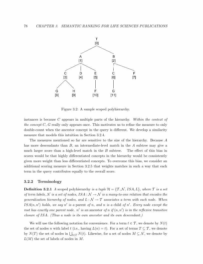
78 CHAPTER 3. SEMANTIC RANKING FOR LIFE SCIENCES PUBLICATIONS
Figure 3.2: A sample scoped polyhierarchy.
instances is because C appears in multiple parts of the hierarchy. Within the context of
the concept C, G really only appears once. This motivates us to refine the measure to only
double-count when the ancestor concept in the query is different. We develop a similarity
measure that models this intuition in Section 3.2.4.
The measures mentioned so far are sensitive to the size of the hierarchy. Because A
has more descendants than B, an intermediate-level match in the A subtree may give a
much larger score than a high-level match in the B subtree. The effect of this bias in
scores would be that highly differentiated concepts in the hierarchy would be consistently
given more weight than less differentiated concepts. To overcome this bias, we consider an
additional scoring measure in Section 3.2.5 that weights matches in such a way that each
term in the query contributes equally to the overall score.
3.2.2 Terminology
Definition 3.2.1 A scoped polyhierarchy is a tuple H = {T ,N , ISA,L}, where T is a set
of term labels, N is a set of nodes, ISA : N → N is a many-to-one relation that encodes the
generalization hierarchy of nodes, and L : N → T associates a term with each node. When
ISA(n, n′) holds, we say n′ is a parent of n, and n is a child of n′. Every node except the
root has exactly one parent node. n′ is an ancestor of n if (n, n′) is in the reflexive transitive
closure of ISA. (Thus a node is its own ancestor and its own descendant.)
We will use the following notation for convenience. For a term t ∈ T , we denote by N(t)
the set of nodes n with label t (i.e., having L(n) = t). For a set of terms T ⊆ T , we denote
by N(T ) the set of nodes in⋃
t∈T N(t). Likewise, for a set of nodes M ⊆ N , we denote by
L(M) the set of labels of nodes in M .
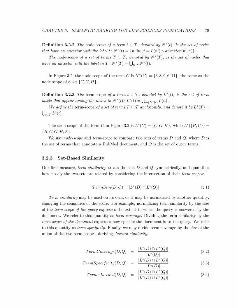
CHAPTER 3. SEMANTIC RANKING FOR LIFE SCIENCES PUBLICATIONS 79
Definition 3.2.2 The node-scope of a term t ∈ T , denoted by N ∗(t), is the set of nodes
that have an ancestor with the label t: N ∗(t) = {n|∃n′, t = L(n′) ∧ ancestor(n′, n)}.
The node-scope of a set of terms T ⊆ T , denoted by N ∗(T ), is the set of nodes that
have an ancestor with the label in T : N ∗(T ) =⋃
t∈T N∗(t).
In Figure 3.2, the node-scope of the term C is N ∗(C) = {3, 8, 9, 6, 11}, the same as the
node scope of a set {C,G,H}.
Definition 3.2.3 The term-scope of a term t ∈ T , denoted by L∗(t), is the set of term
labels that appear among the nodes in N ∗(t): L∗(t) =⋃
n∈N∗(t) L(n).
We define the term-scope of a set of terms T ⊆ T analogously, and denote it by L∗(T ) =⋃
t∈T L∗(t).
The term-scope of the term C in Figure 3.2 is L∗(C) = {C,G,H}, while L∗({B,C}) =
{B,C,G,H, F}.
We use node-scope and term-scope to compare two sets of terms D and Q, where D is
the set of terms that annotate a PubMed document, and Q is the set of query terms.
3.2.3 Set-Based Similarity
Our first measure, term similarity, treats the sets D and Q symmetrically, and quantifies
how closely the two sets are related by considering the intersection of their term-scopes:
TermSim(D,Q) = |L∗(D) ∩ L∗(Q)| (3.1)
Term similarity may be used on its own, or it may be normalized by another quantity,
changing the semantics of the score. For example, normalizing term similarity by the size
of the term-scope of the query expresses the extent to which the query is answered by the
document. We refer to this quantity as term coverage. Dividing the term similarity by the
term-scope of the document expresses how specific the document is to the query. We refer
to this quantity as term specificity. Finally, we may divide term coverage by the size of the
union of the two term scopes, deriving Jaccard similarity.
TermCoverage(D,Q) =|L∗(D) ∩ L∗(Q)|
|L∗(Q)|(3.2)
TermSpecificity(D,Q) =|L∗(D) ∩ L∗(Q)|
|L∗(D)|(3.3)
TermsJaccard(D,Q) =|L∗(D) ∩ L∗(Q)|
|L∗(D) ∪ L∗(Q)|(3.4)
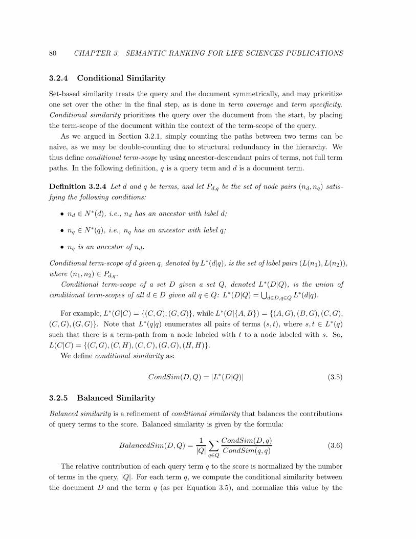
80 CHAPTER 3. SEMANTIC RANKING FOR LIFE SCIENCES PUBLICATIONS
3.2.4 Conditional Similarity
Set-based similarity treats the query and the document symmetrically, and may prioritize
one set over the other in the final step, as is done in term coverage and term specificity.
Conditional similarity prioritizes the query over the document from the start, by placing
the term-scope of the document within the context of the term-scope of the query.
As we argued in Section 3.2.1, simply counting the paths between two terms can be
naive, as we may be double-counting due to structural redundancy in the hierarchy. We
thus define conditional term-scope by using ancestor-descendant pairs of terms, not full term
paths. In the following definition, q is a query term and d is a document term.
Definition 3.2.4 Let d and q be terms, and let Pd,q be the set of node pairs (nd, nq) satis-
fying the following conditions:
• nd ∈ N∗(d), i.e., nd has an ancestor with label d;
• nq ∈ N∗(q), i.e., nq has an ancestor with label q;
• nq is an ancestor of nd.
Conditional term-scope of d given q, denoted by L∗(d|q), is the set of label pairs (L(n1), L(n2)),
where (n1, n2) ∈ Pd,q.
Conditional term-scope of a set D given a set Q, denoted L∗(D|Q), is the union of
conditional term-scopes of all d ∈ D given all q ∈ Q: L∗(D|Q) =⋃
d∈D,q∈Q L∗(d|q).
For example, L∗(G|C) = {(C,G), (G,G)}, while L∗(G|{A,B}) = {(A,G), (B,G), (C,G),
(C,G), (G,G)}. Note that L∗(q|q) enumerates all pairs of terms (s, t), where s, t ∈ L∗(q)
such that there is a term-path from a node labeled with t to a node labeled with s. So,
L(C|C) = {(C,G), (C,H), (C,C), (G,G), (H,H)}.
We define conditional similarity as:
CondSim(D,Q) = |L∗(D|Q)| (3.5)
3.2.5 Balanced Similarity
Balanced similarity is a refinement of conditional similarity that balances the contributions
of query terms to the score. Balanced similarity is given by the formula:
BalancedSim(D,Q) =1
|Q|
∑
q∈Q
CondSim(D, q)
CondSim(q, q)(3.6)
The relative contribution of each query term q to the score is normalized by the number
of terms in the query, |Q|. For each term q, we compute the conditional similarity between
the document D and the term q (as per Equation 3.5), and normalize this value by the
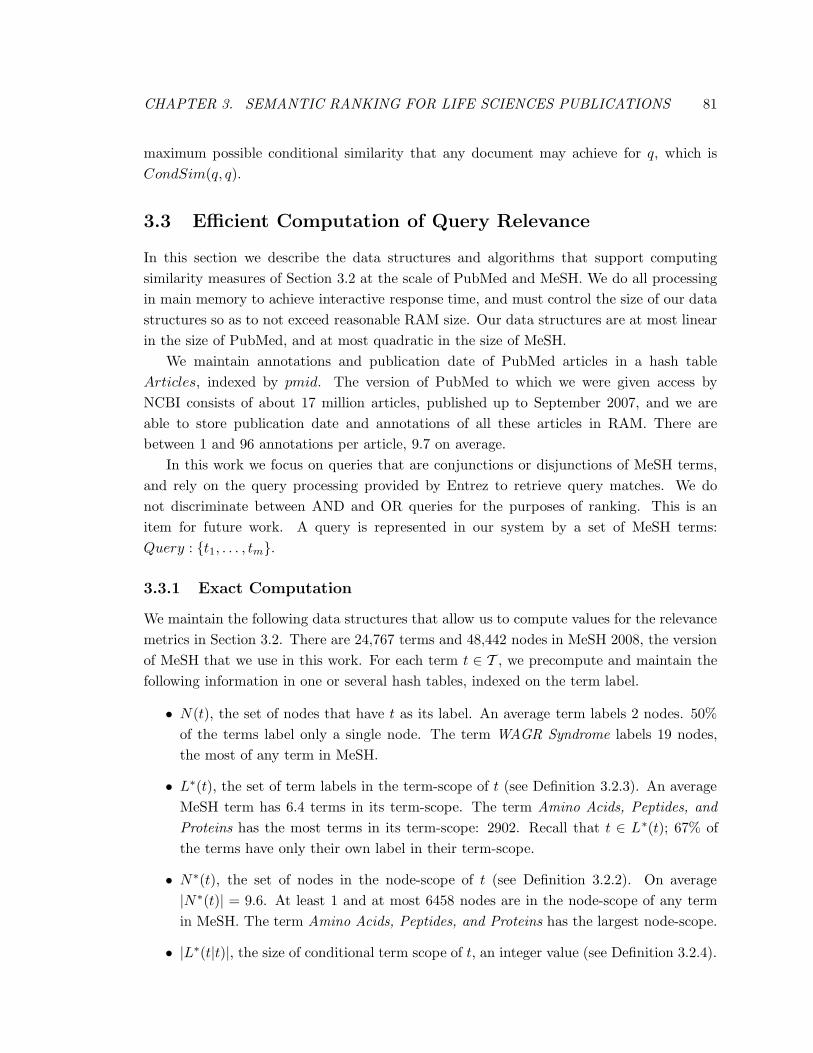
CHAPTER 3. SEMANTIC RANKING FOR LIFE SCIENCES PUBLICATIONS 81
maximum possible conditional similarity that any document may achieve for q, which is
CondSim(q, q).
3.3 Efficient Computation of Query Relevance
In this section we describe the data structures and algorithms that support computing
similarity measures of Section 3.2 at the scale of PubMed and MeSH. We do all processing
in main memory to achieve interactive response time, and must control the size of our data
structures so as to not exceed reasonable RAM size. Our data structures are at most linear
in the size of PubMed, and at most quadratic in the size of MeSH.
We maintain annotations and publication date of PubMed articles in a hash table
Articles, indexed by pmid. The version of PubMed to which we were given access by
NCBI consists of about 17 million articles, published up to September 2007, and we are
able to store publication date and annotations of all these articles in RAM. There are
between 1 and 96 annotations per article, 9.7 on average.
In this work we focus on queries that are conjunctions or disjunctions of MeSH terms,
and rely on the query processing provided by Entrez to retrieve query matches. We do
not discriminate between AND and OR queries for the purposes of ranking. This is an
item for future work. A query is represented in our system by a set of MeSH terms:
Query : {t1, . . . , tm}.
3.3.1 Exact Computation
We maintain the following data structures that allow us to compute values for the relevance
metrics in Section 3.2. There are 24,767 terms and 48,442 nodes in MeSH 2008, the version
of MeSH that we use in this work. For each term t ∈ T , we precompute and maintain the
following information in one or several hash tables, indexed on the term label.
• N(t), the set of nodes that have t as its label. An average term labels 2 nodes. 50%
of the terms label only a single node. The term WAGR Syndrome labels 19 nodes,
the most of any term in MeSH.
• L∗(t), the set of term labels in the term-scope of t (see Definition 3.2.3). An average
MeSH term has 6.4 terms in its term-scope. The term Amino Acids, Peptides, and
Proteins has the most terms in its term-scope: 2902. Recall that t ∈ L∗(t); 67% of
the terms have only their own label in their term-scope.
• N∗(t), the set of nodes in the node-scope of t (see Definition 3.2.2). On average
|N∗(t)| = 9.6. At least 1 and at most 6458 nodes are in the node-scope of any term
in MeSH. The term Amino Acids, Peptides, and Proteins has the largest node-scope.
• |L∗(t|t)|, the size of conditional term scope of t, an integer value (see Definition 3.2.4).
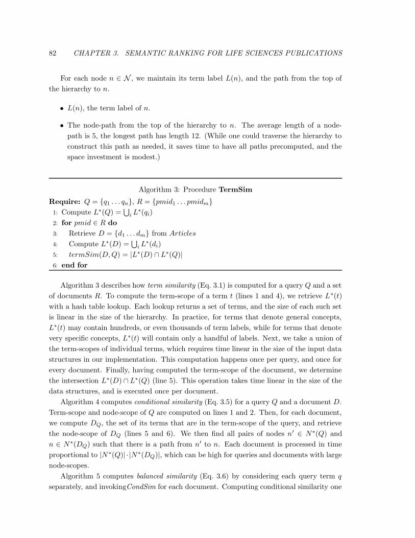
82 CHAPTER 3. SEMANTIC RANKING FOR LIFE SCIENCES PUBLICATIONS
For each node n ∈ N , we maintain its term label L(n), and the path from the top of
the hierarchy to n.
• L(n), the term label of n.
• The node-path from the top of the hierarchy to n. The average length of a node-
path is 5, the longest path has length 12. (While one could traverse the hierarchy to
construct this path as needed, it saves time to have all paths precomputed, and the
space investment is modest.)
Algorithm 3: Procedure TermSim
Require: Q = {q1 . . . qn}, R = {pmid1 . . . pmidm}
1: Compute L∗(Q) =⋃
i L∗(qi)
2: for pmid ∈ R do
3: Retrieve D = {d1 . . . dm} from Articles
4: Compute L∗(D) =⋃
i L∗(di)
5: termSim(D,Q) = |L∗(D) ∩ L∗(Q)|
6: end for
Algorithm 3 describes how term similarity (Eq. 3.1) is computed for a query Q and a set
of documents R. To compute the term-scope of a term t (lines 1 and 4), we retrieve L∗(t)
with a hash table lookup. Each lookup returns a set of terms, and the size of each such set
is linear in the size of the hierarchy. In practice, for terms that denote general concepts,
L∗(t) may contain hundreds, or even thousands of term labels, while for terms that denote
very specific concepts, L∗(t) will contain only a handful of labels. Next, we take a union of
the term-scopes of individual terms, which requires time linear in the size of the input data
structures in our implementation. This computation happens once per query, and once for
every document. Finally, having computed the term-scope of the document, we determine
the intersection L∗(D) ∩ L∗(Q) (line 5). This operation takes time linear in the size of the
data structures, and is executed once per document.
Algorithm 4 computes conditional similarity (Eq. 3.5) for a query Q and a document D.
Term-scope and node-scope of Q are computed on lines 1 and 2. Then, for each document,
we compute DQ, the set of its terms that are in the term-scope of the query, and retrieve
the node-scope of DQ (lines 5 and 6). We then find all pairs of nodes n′ ∈ N∗(Q) and
n ∈ N∗(DQ) such that there is a path from n′ to n. Each document is processed in time
proportional to |N ∗(Q)| · |N ∗(DQ)|, which can be high for queries and documents with large
node-scopes.
Algorithm 5 computes balanced similarity (Eq. 3.6) by considering each query term q
separately, and invokingCondSim for each document. Computing conditional similarity one
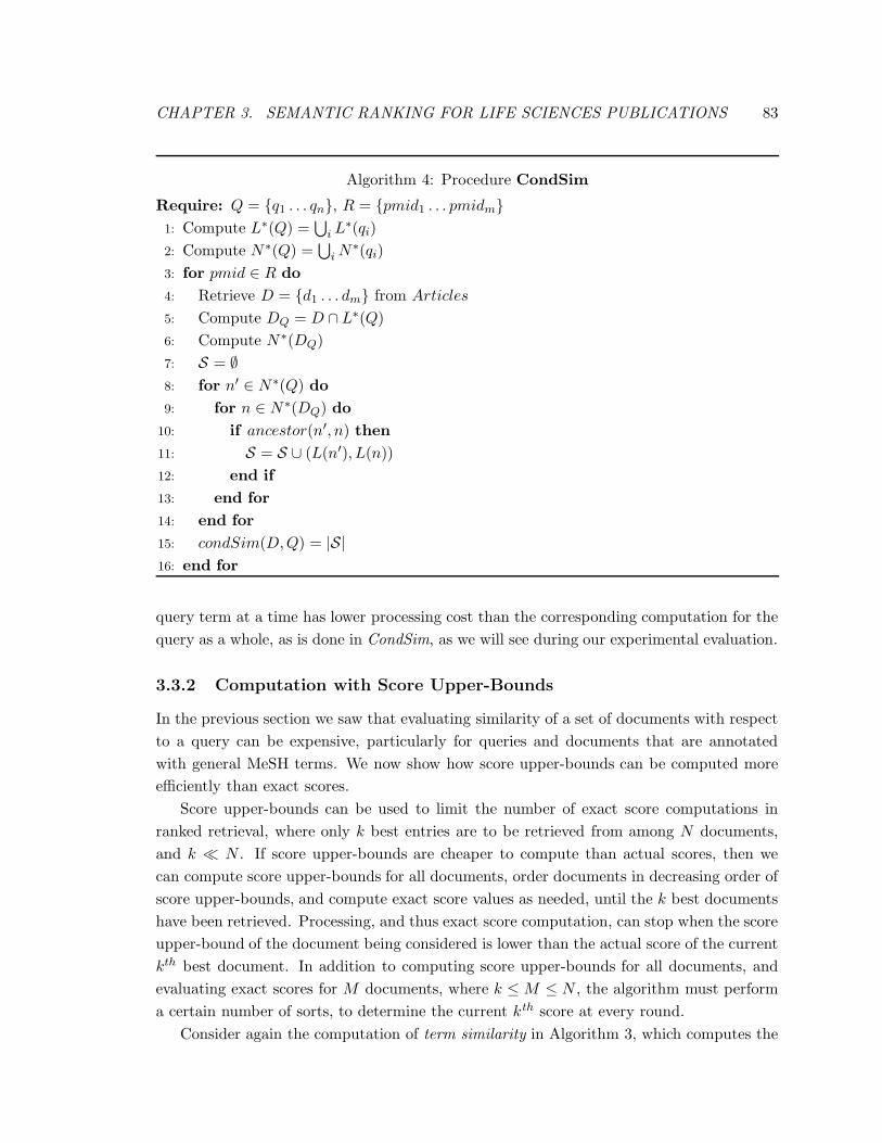
CHAPTER 3. SEMANTIC RANKING FOR LIFE SCIENCES PUBLICATIONS 83
Algorithm 4: Procedure CondSim
Require: Q = {q1 . . . qn}, R = {pmid1 . . . pmidm}
1: Compute L∗(Q) =⋃
i L∗(qi)
2: Compute N ∗(Q) =⋃
i N∗(qi)
3: for pmid ∈ R do
4: Retrieve D = {d1 . . . dm} from Articles
5: Compute DQ = D ∩ L∗(Q)
6: Compute N ∗(DQ)
7: S = ∅
8: for n′ ∈ N∗(Q) do
9: for n ∈ N ∗(DQ) do
10: if ancestor(n′, n) then
11: S = S ∪ (L(n′), L(n))
12: end if
13: end for
14: end for
15: condSim(D,Q) = |S|
16: end for
query term at a time has lower processing cost than the corresponding computation for the
query as a whole, as is done in CondSim, as we will see during our experimental evaluation.
3.3.2 Computation with Score Upper-Bounds
In the previous section we saw that evaluating similarity of a set of documents with respect
to a query can be expensive, particularly for queries and documents that are annotated
with general MeSH terms. We now show how score upper-bounds can be computed more
efficiently than exact scores.
Score upper-bounds can be used to limit the number of exact score computations in
ranked retrieval, where only k best entries are to be retrieved from among N documents,
and k � N . If score upper-bounds are cheaper to compute than actual scores, then we
can compute score upper-bounds for all documents, order documents in decreasing order of
score upper-bounds, and compute exact score values as needed, until the k best documents
have been retrieved. Processing, and thus exact score computation, can stop when the score
upper-bound of the document being considered is lower than the actual score of the current
kth best document. In addition to computing score upper-bounds for all documents, and
evaluating exact scores for M documents, where k ≤M ≤ N , the algorithm must perform
a certain number of sorts, to determine the current kth score at every round.
Consider again the computation of term similarity in Algorithm 3, which computes the
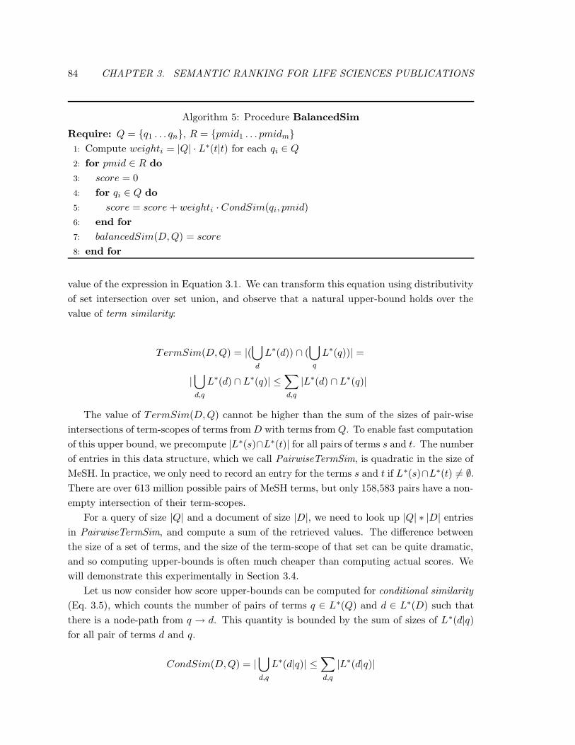
84 CHAPTER 3. SEMANTIC RANKING FOR LIFE SCIENCES PUBLICATIONS
Algorithm 5: Procedure BalancedSim
Require: Q = {q1 . . . qn}, R = {pmid1 . . . pmidm}
1: Compute weighti = |Q| · L∗(t|t) for each qi ∈ Q
2: for pmid ∈ R do
3: score = 0
4: for qi ∈ Q do
5: score = score + weighti · CondSim(qi, pmid)
6: end for
7: balancedSim(D,Q) = score
8: end for
value of the expression in Equation 3.1. We can transform this equation using distributivity
of set intersection over set union, and observe that a natural upper-bound holds over the
value of term similarity:
TermSim(D,Q) = |(⋃
d
L∗(d)) ∩ (⋃
q
L∗(q))| =
|⋃
d,q
L∗(d) ∩ L∗(q)| ≤∑
d,q
|L∗(d) ∩ L∗(q)|
The value of TermSim(D,Q) cannot be higher than the sum of the sizes of pair-wise
intersections of term-scopes of terms from D with terms from Q. To enable fast computation
of this upper bound, we precompute |L∗(s)∩L∗(t)| for all pairs of terms s and t. The number
of entries in this data structure, which we call PairwiseTermSim, is quadratic in the size of
MeSH. In practice, we only need to record an entry for the terms s and t if L∗(s)∩L∗(t) 6= ∅.
There are over 613 million possible pairs of MeSH terms, but only 158,583 pairs have a non-
empty intersection of their term-scopes.
For a query of size |Q| and a document of size |D|, we need to look up |Q| ∗ |D| entries
in PairwiseTermSim, and compute a sum of the retrieved values. The difference between
the size of a set of terms, and the size of the term-scope of that set can be quite dramatic,
and so computing upper-bounds is often much cheaper than computing actual scores. We
will demonstrate this experimentally in Section 3.4.
Let us now consider how score upper-bounds can be computed for conditional similarity
(Eq. 3.5), which counts the number of pairs of terms q ∈ L∗(Q) and d ∈ L∗(D) such that
there is a node-path from q → d. This quantity is bounded by the sum of sizes of L∗(d|q)
for all pair of terms d and q.
CondSim(D,Q) = |⋃
d,q
L∗(d|q)| ≤∑
d,q
|L∗(d|q)|
CHAPTER 3. SEMANTIC RANKING FOR LIFE SCIENCES PUBLICATIONS 85
To facilitate the computation of this upper-bound, we store the value of L∗(s|t) for
all pairs of terms s and t with intersecting term-scopes. We call this data structure
PairwiseCondSim. This data structure has the same number of entries as PairwiseTerm-
Sim.
Finally, for balanced similarity, we observe that:
BalSim(D,Q) =1
|Q|
∑
q
L∗(D|q)|
L∗(q|q)=
1
|Q|
∑
q,d
L∗(d|q)
L∗(q|q)
We re-use the PairwiseCondSim data structure for the computation of score-upper
bounds for balanced similarity. We evaluate the performance improvements achieved by
using score upper-bounds for ranked retrieval in Section 3.4.
3.3.3 Adaptive Skyline Computation with Upper-Bounds
As we argued in the Introduction, it is sometimes important to present more than a handful
of query results. We propose to use a two-dimensional skyline visualization [Borzsonyi et
al., 2001] that is based on the familiar concept of dominance. A point in multi-dimensional
space is said to belong to the skyline if it is not dominated by any other point, i.e., if no other
point is as good or better in all dimensions, and strictly better in at least one dimension.
A skyline contour is defined inductively as follows:
• A point belongs to the first skyline contour if and only if it belongs to the skyline of
the whole data set.
• A point belongs to the kth contour if and only if it belongs to the skyline of the data
set obtained by removing points from the first through k − 1st contours.
Skyline contours are useful for highlighting points that are close to the skyline, and that
might be of interest to the user.
Publication date is a natural attribute in which to consider bibliography matches, and
we use it as the x-axis of our visualization. The y-axis corresponds to one of the similarity
measures described in Section 3.2. Figure 3.3 shows a skyline of results for the query G-
Protein-Coupled receptors, for term specificity with 5 skyline contours. Points of highest
quality are close to the origin on the x-axis and away from the origin on the y-axis. Points
on the first contour are marked in white, points on the second contour are beige, and point
on the last contour are red. When points are selected using the mouse, a window showing
the full citation is displayed.
Our prototype implementation is running outside of the NCBI infrastructure, and we are
using the Entrez query API, eUtils, to evaluate queries, and receive back ids of PubMed
articles that match the query. The eUtils API can be asked to return query results in
order of publication date. NCBI requests that large result sets be retrieved in batches, so
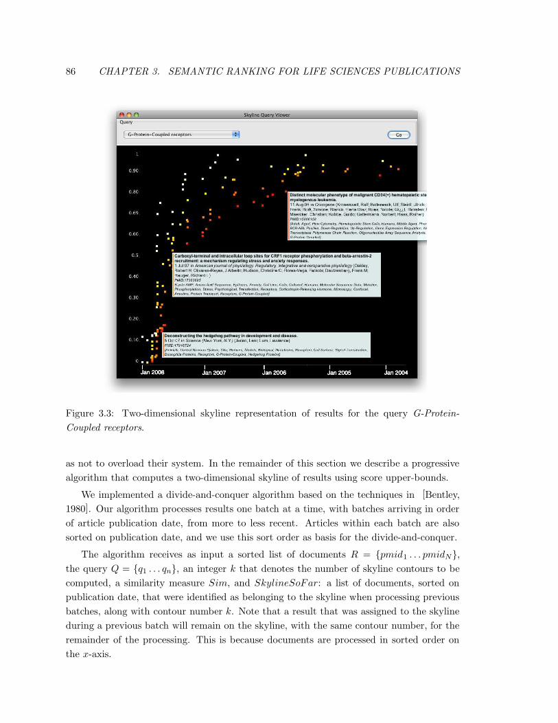
86 CHAPTER 3. SEMANTIC RANKING FOR LIFE SCIENCES PUBLICATIONS
Figure 3.3: Two-dimensional skyline representation of results for the query G-Protein-
Coupled receptors.
as not to overload their system. In the remainder of this section we describe a progressive
algorithm that computes a two-dimensional skyline of results using score upper-bounds.
We implemented a divide-and-conquer algorithm based on the techniques in [Bentley,
1980]. Our algorithm processes results one batch at a time, with batches arriving in order
of article publication date, from more to less recent. Articles within each batch are also
sorted on publication date, and we use this sort order as basis for the divide-and-conquer.
The algorithm receives as input a sorted list of documents R = {pmid1 . . . pmidN},
the query Q = {q1 . . . qn}, an integer k that denotes the number of skyline contours to be
computed, a similarity measure Sim, and SkylineSoFar: a list of documents, sorted on
publication date, that were identified as belonging to the skyline when processing previous
batches, along with contour number k. Note that a result that was assigned to the skyline
during a previous batch will remain on the skyline, with the same contour number, for the
remainder of the processing. This is because documents are processed in sorted order on
the x-axis.
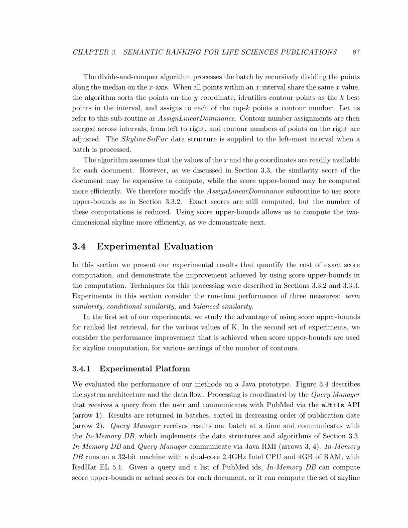
CHAPTER 3. SEMANTIC RANKING FOR LIFE SCIENCES PUBLICATIONS 87
The divide-and-conquer algorithm processes the batch by recursively dividing the points
along the median on the x-axis. When all points within an x-interval share the same x value,
the algorithm sorts the points on the y coordinate, identifies contour points as the k best
points in the interval, and assigns to each of the top-k points a contour number. Let us
refer to this sub-routine as AssignLinearDominance. Contour number assignments are then
merged across intervals, from left to right, and contour numbers of points on the right are
adjusted. The SkylineSoFar data structure is supplied to the left-most interval when a
batch is processed.
The algorithm assumes that the values of the x and the y coordinates are readily available
for each document. However, as we discussed in Section 3.3, the similarity score of the
document may be expensive to compute, while the score upper-bound may be computed
more efficiently. We therefore modify the AssignLinearDominance subroutine to use score
upper-bounds as in Section 3.3.2. Exact scores are still computed, but the number of
these computations is reduced. Using score upper-bounds allows us to compute the two-
dimensional skyline more efficiently, as we demonstrate next.
3.4 Experimental Evaluation
In this section we present our experimental results that quantify the cost of exact score
computation, and demonstrate the improvement achieved by using score upper-bounds in
the computation. Techniques for this processing were described in Sections 3.3.2 and 3.3.3.
Experiments in this section consider the run-time performance of three measures: term
similarity, conditional similarity, and balanced similarity.
In the first set of our experiments, we study the advantage of using score upper-bounds
for ranked list retrieval, for the various values of K. In the second set of experiments, we
consider the performance improvement that is achieved when score upper-bounds are used
for skyline computation, for various settings of the number of contours.
3.4.1 Experimental Platform
We evaluated the performance of our methods on a Java prototype. Figure 3.4 describes
the system architecture and the data flow. Processing is coordinated by the Query Manager
that receives a query from the user and communicates with PubMed via the eUtils API
(arrow 1). Results are returned in batches, sorted in decreasing order of publication date
(arrow 2). Query Manager receives results one batch at a time and communicates with
the In-Memory DB, which implements the data structures and algorithms of Section 3.3.
In-Memory DB and Query Manager communicate via Java RMI (arrows 3, 4). In-Memory
DB runs on a 32-bit machine with a dual-core 2.4GHz Intel CPU and 4GB of RAM, with
RedHat EL 5.1. Given a query and a list of PubMed ids, In-Memory DB can compute
score upper-bounds or actual scores for each document, or it can compute the set of skyline
88 CHAPTER 3. SEMANTIC RANKING FOR LIFE SCIENCES PUBLICATIONS
Figure 3.4: System architecture.
contours. Results are read by Query Manager (arrow 4), which can optionally pass them
to the visualization component.
For the purposes of our evaluation all processing was done by In-Memory DB, to reduce
communication cost. When a system like ours is deployed, some of the processing, e.g. sky-
line computation, can be moved to the client to reduce server load. All performance results
are based on measuring processing times inside In-Memory DB. We report performance in
terms of wall-clock time. All results are averages of three executions.
3.4.2 Workload
Our performance experiments are based on a workload of 150 queries. We were unable
to get a real PubMed query workload from NCBI due to privacy regulations, and so we
generated the workload based on pairwise co-occurrence of terms in annotations of PubMed
articles. The rationale is that, if two or more terms are commonly used to annotate the
same document, then these terms are semantically related and may be used together in a
query. We generated the query workload as follows.
We took the set of all PubMed documents that were published during the month of
January 2007, 124,413 documents in all, and computed pair-wise co-occurrence of terms
in those documents. 20,848 out of a total of 24,767 MeSH terms are used to annotate
documents in this sample. For all pairs of terms t1 and t2, we recorded the number of
documents that are annotated with both t1 and t2, and compared this to the number of
documents annotated with t1 alone, and with t2 alone. We refer to the sizes of these three
document sets as D(t1 ∧ t2), D(t1), and D(t2), respectively.
Over 2.5 million pairs of terms were used together to annotate at least one document
in our set. From among those, we selected pairs that contained terms that were neither too
common not too uncommon. We removed terms that annotate more than 100 documents
and fewer than 3 documents in the sample. Extremely common terms, such as Human
and Female are likely too general to be used in a query. Very uncommon terms may be
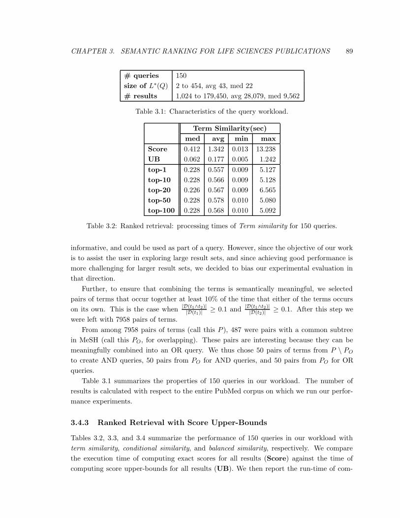
CHAPTER 3. SEMANTIC RANKING FOR LIFE SCIENCES PUBLICATIONS 89
# queries 150
size of L∗(Q) 2 to 454, avg 43, med 22
# results 1,024 to 179,450, avg 28,079, med 9,562
Table 3.1: Characteristics of the query workload.
Term Similarity(sec)
med avg min max
Score 0.412 1.342 0.013 13.238
UB 0.062 0.177 0.005 1.242
top-1 0.228 0.557 0.009 5.127
top-10 0.228 0.566 0.009 5.128
top-20 0.226 0.567 0.009 6.565
top-50 0.228 0.578 0.010 5.080
top-100 0.228 0.568 0.010 5.092
Table 3.2: Ranked retrieval: processing times of Term similarity for 150 queries.
informative, and could be used as part of a query. However, since the objective of our work
is to assist the user in exploring large result sets, and since achieving good performance is
more challenging for larger result sets, we decided to bias our experimental evaluation in
that direction.
Further, to ensure that combining the terms is semantically meaningful, we selected
pairs of terms that occur together at least 10% of the time that either of the terms occurs
on its own. This is the case when |D(t1∧t2)||D(t1)| ≥ 0.1 and |D(t1∧t2)|
|D(t2)| ≥ 0.1. After this step we
were left with 7958 pairs of terms.
From among 7958 pairs of terms (call this P ), 487 were pairs with a common subtree
in MeSH (call this PO, for overlapping). These pairs are interesting because they can be
meaningfully combined into an OR query. We thus chose 50 pairs of terms from P \ PO
to create AND queries, 50 pairs from PO for AND queries, and 50 pairs from PO for OR
queries.
Table 3.1 summarizes the properties of 150 queries in our workload. The number of
results is calculated with respect to the entire PubMed corpus on which we run our perfor-
mance experiments.
3.4.3 Ranked Retrieval with Score Upper-Bounds
Tables 3.2, 3.3, and 3.4 summarize the performance of 150 queries in our workload with
term similarity, conditional similarity, and balanced similarity, respectively. We compare
the execution time of computing exact scores for all results (Score) against the time of
computing score upper-bounds for all results (UB). We then report the run-time of com-
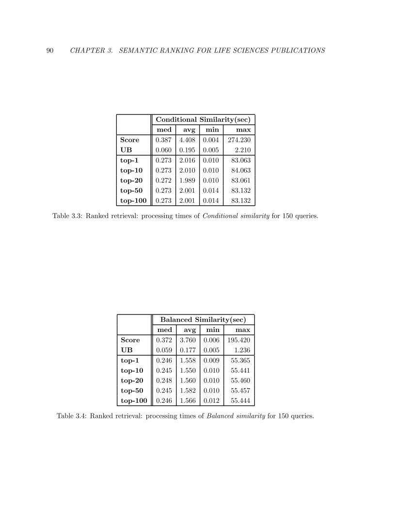
90 CHAPTER 3. SEMANTIC RANKING FOR LIFE SCIENCES PUBLICATIONS
Conditional Similarity(sec)
med avg min max
Score 0.387 4.408 0.004 274.230
UB 0.060 0.195 0.005 2.210
top-1 0.273 2.016 0.010 83.063
top-10 0.273 2.010 0.010 84.063
top-20 0.272 1.989 0.010 83.061
top-50 0.273 2.001 0.014 83.132
top-100 0.273 2.001 0.014 83.132
Table 3.3: Ranked retrieval: processing times of Conditional similarity for 150 queries.
Balanced Similarity(sec)
med avg min max
Score 0.372 3.760 0.006 195.420
UB 0.059 0.177 0.005 1.236
top-1 0.246 1.558 0.009 55.365
top-10 0.245 1.550 0.010 55.441
top-20 0.248 1.560 0.010 55.460
top-50 0.245 1.582 0.010 55.457
top-100 0.246 1.566 0.012 55.444
Table 3.4: Ranked retrieval: processing times of Balanced similarity for 150 queries.
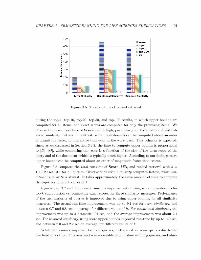
CHAPTER 3. SEMANTIC RANKING FOR LIFE SCIENCES PUBLICATIONS 91
Figure 3.5: Total runtime of ranked retrieval.
puting the top-1, top-10, top-20, top-50, and top-100 results, in which upper bounds are
computed for all items, and exact scores are computed for only the promising items. We
observe that execution time of Score can be high, particularly for the conditional and bal-
anced similarity metrics. In contrast, score upper-bounds can be computed about an order
of magnitude faster, in interactive time even in the worst case. This behavior is expected,
since, as we discussed in Section 3.3.2, the time to compute upper bounds is proportional
to |D| · |Q|, while computing the score is a function of the size of the term-scope of the
query and of the document, which is typically much higher. According to our findings score
upper-bounds can be computed about an order of magnitude faster than scores.
Figure 3.5 compares the total run-time of Score, UB, and ranked retrieval with k =
1, 10, 20, 50, 100, for all queries. Observe that term similarity computes fastest, while con-
ditional similarity is slowest. It takes approximately the same amount of time to compute
the top-k for different values of k.
Figures 3.6, 3.7 and 3.8 present run-time improvement of using score upper-bounds for
top-k computation vs. computing exact scores, for three similarity measures. Performance
of the vast majority of queries is improved due to using upper-bounds, for all similarity
measures. The actual run-time improvement was up to 9.1 sec for term similarity, and
between 0.7 and 0.8 sec on average for different values of k. For conditional similarity, the
improvement was up to a dramatic 191 sec, and the average improvement was about 2.4
sec. For balanced similarity, using score upper-bounds improved run-time by up to 140 sec,
and between 2.0 and 2.2 sec on average, for different values of k.
While performance improved for most queries, it degraded for some queries due to the
overhead of sorting. This overhead was noticeable only in short-running queries, and abso-
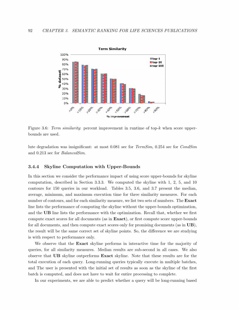
92 CHAPTER 3. SEMANTIC RANKING FOR LIFE SCIENCES PUBLICATIONS
Figure 3.6: Term similarity: percent improvement in runtime of top-k when score upper-
bounds are used.
lute degradation was insignificant: at most 0.081 sec for TermSim, 0.254 sec for CondSim
and 0.213 sec for BalancedSim.
3.4.4 Skyline Computation with Upper-Bounds
In this section we consider the performance impact of using score upper-bounds for skyline
computation, described in Section 3.3.3. We computed the skyline with 1, 2, 5, and 10
contours for 150 queries in our workload. Tables 3.5, 3.6, and 3.7 present the median,
average, minimum, and maximum execution time for three similarity measures. For each
number of contours, and for each similarity measure, we list two sets of numbers. The Exact
line lists the performance of computing the skyline without the upper-bounds optimization,
and the UB line lists the performance with the optimization. Recall that, whether we first
compute exact scores for all documents (as in Exact), or first compute score upper-bounds
for all documents, and then compute exact scores only for promising documents (as in UB),
the result will be the same correct set of skyline points. So, the difference we are studying
is with respect to performance only.
We observe that the Exact skyline performs in interactive time for the majority of
queries, for all similarity measures. Median results are sub-second in all cases. We also
observe that UB skyline outperforms Exact skyline. Note that these results are for the
total execution of each query. Long-running queries typically execute in multiple batches,
and The user is presented with the initial set of results as soon as the skyline of the first
batch is computed, and does not have to wait for entire processing to complete.
In our experiments, we are able to predict whether a query will be long-running based
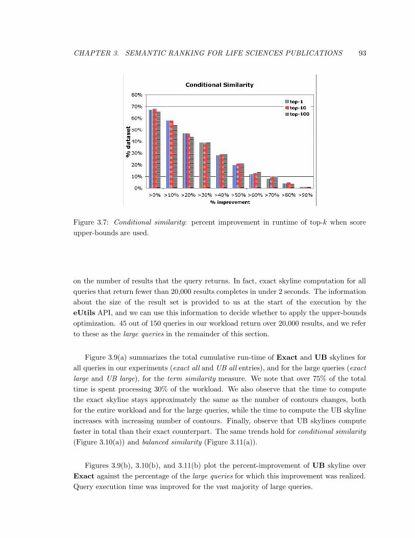
CHAPTER 3. SEMANTIC RANKING FOR LIFE SCIENCES PUBLICATIONS 93
Figure 3.7: Conditional similarity: percent improvement in runtime of top-k when score
upper-bounds are used.
on the number of results that the query returns. In fact, exact skyline computation for all
queries that return fewer than 20,000 results completes in under 2 seconds. The information
about the size of the result set is provided to us at the start of the execution by the
eUtils API, and we can use this information to decide whether to apply the upper-bounds
optimization. 45 out of 150 queries in our workload return over 20,000 results, and we refer
to these as the large queries in the remainder of this section.
Figure 3.9(a) summarizes the total cumulative run-time of Exact and UB skylines for
all queries in our experiments (exact all and UB all entries), and for the large queries (exact
large and UB large), for the term similarity measure. We note that over 75% of the total
time is spent processing 30% of the workload. We also observe that the time to compute
the exact skyline stays approximately the same as the number of contours changes, both
for the entire workload and for the large queries, while the time to compute the UB skyline
increases with increasing number of contours. Finally, observe that UB skylines compute
faster in total than their exact counterpart. The same trends hold for conditional similarity
(Figure 3.10(a)) and balanced similarity (Figure 3.11(a)).
Figures 3.9(b), 3.10(b), and 3.11(b) plot the percent-improvement of UB skyline over
Exact against the percentage of the large queries for which this improvement was realized.
Query execution time was improved for the vast majority of large queries.
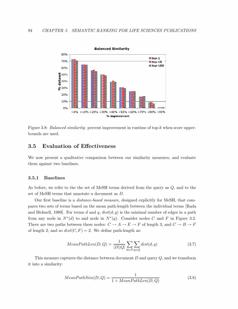
94 CHAPTER 3. SEMANTIC RANKING FOR LIFE SCIENCES PUBLICATIONS
Figure 3.8: Balanced similarity: percent improvement in runtime of top-k when score upper-
bounds are used.
3.5 Evaluation of Effectiveness
We now present a qualitative comparison between our similarity measures, and evaluate
them against two baselines.
3.5.1 Baselines
As before, we refer to the the set of MeSH terms derived from the query as Q, and to the
set of MeSH terms that annotate a document as D.
Our first baseline is a distance-based measure, designed explicitly for MeSH, that com-
pares two sets of terms based on the mean path-length between the individual terms [Rada
and Bicknell, 1989]. For terms d and q, dist(d, q) is the minimal number of edges in a path
from any node in N ∗(d) to and node in N ∗(q). Consider nodes C and F in Figure 3.2.
There are two paths between these nodes: C → A→ E → F of length 3, and C → B → F
of length 2, and so dist(C,F ) = 2. We define path-length as:
MeanPathLen(D,Q) =1
|D||Q|
∑
d∈D
∑
q∈Q
dist(d, q) (3.7)
This measure captures the distance between document D and query Q, and we transform
it into a similarity:
MeanPathSim(D,Q) =1
1 + MeanPathLen(D,Q)(3.8)
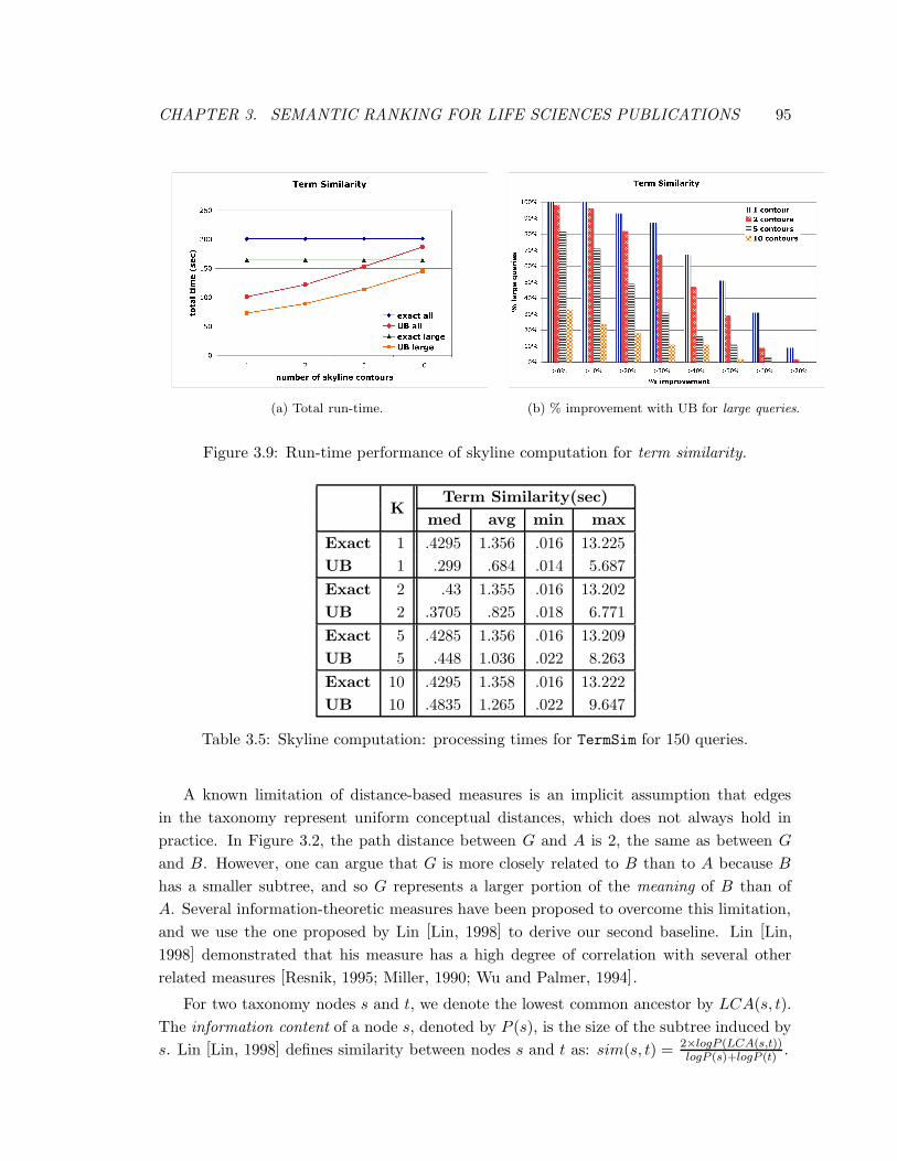
CHAPTER 3. SEMANTIC RANKING FOR LIFE SCIENCES PUBLICATIONS 95
(a) Total run-time. (b) % improvement with UB for large queries.
Figure 3.9: Run-time performance of skyline computation for term similarity.
KTerm Similarity(sec)
med avg min max
Exact 1 .4295 1.356 .016 13.225
UB 1 .299 .684 .014 5.687
Exact 2 .43 1.355 .016 13.202
UB 2 .3705 .825 .018 6.771
Exact 5 .4285 1.356 .016 13.209
UB 5 .448 1.036 .022 8.263
Exact 10 .4295 1.358 .016 13.222
UB 10 .4835 1.265 .022 9.647
Table 3.5: Skyline computation: processing times for TermSim for 150 queries.
A known limitation of distance-based measures is an implicit assumption that edges
in the taxonomy represent uniform conceptual distances, which does not always hold in
practice. In Figure 3.2, the path distance between G and A is 2, the same as between G
and B. However, one can argue that G is more closely related to B than to A because B
has a smaller subtree, and so G represents a larger portion of the meaning of B than of
A. Several information-theoretic measures have been proposed to overcome this limitation,
and we use the one proposed by Lin [Lin, 1998] to derive our second baseline. Lin [Lin,
1998] demonstrated that his measure has a high degree of correlation with several other
related measures [Resnik, 1995; Miller, 1990; Wu and Palmer, 1994].
For two taxonomy nodes s and t, we denote the lowest common ancestor by LCA(s, t).
The information content of a node s, denoted by P (s), is the size of the subtree induced by
s. Lin [Lin, 1998] defines similarity between nodes s and t as: sim(s, t) = 2×logP (LCA(s,t))logP (s)+logP (t) .
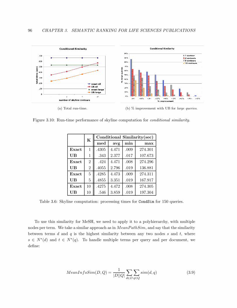
96 CHAPTER 3. SEMANTIC RANKING FOR LIFE SCIENCES PUBLICATIONS
(a) Total run-time. (b) % improvement with UB for large queries.
Figure 3.10: Run-time performance of skyline computation for conditional similarity.
KConditional Similarity(sec)
med avg min max
Exact 1 .4305 4.471 .009 274.301
UB 1 .343 2.377 .017 107.673
Exact 2 .424 4.471 .008 274.296
UB 2 .4055 2.796 .019 136.881
Exact 5 .4285 4.473 .009 274.311
UB 5 .4855 3.351 .019 167.917
Exact 10 .4275 4.472 .008 274.305
UB 10 .546 3.859 .019 197.304
Table 3.6: Skyline computation: processing times for CondSim for 150 queries.
To use this similarity for MeSH, we need to apply it to a polyhierarchy, with multiple
nodes per term. We take a similar approach as in MeanPathSim, and say that the similarity
between terms d and q is the highest similarity between any two nodes s and t, where
s ∈ N∗(d) and t ∈ N ∗(q). To handle multiple terms per query and per document, we
define:
MeanInfoSim(D,Q) =1
|D||Q|
∑
d∈D
∑
q∈Q
sim(d, q) (3.9)
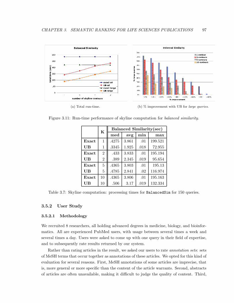
CHAPTER 3. SEMANTIC RANKING FOR LIFE SCIENCES PUBLICATIONS 97
(a) Total run-time. (b) % improvement with UB for large queries.
Figure 3.11: Run-time performance of skyline computation for balanced similarity.
KBalanced Similarity(sec)
med avg min max
Exact 1 .4275 3.861 .01 199.521
UB 1 .3345 1.925 .018 72.955
Exact 2 .433 3.833 .01 195.194
UB 2 .389 2.345 .019 95.654
Exact 5 .4365 3.803 .01 195.13
UB 5 .4785 2.841 .02 116.974
Exact 10 .4365 3.806 .01 195.163
UB 10 .506 3.17 .019 132.334
Table 3.7: Skyline computation: processing times for BalancedSim for 150 queries.
3.5.2 User Study
3.5.2.1 Methodology
We recruited 8 researchers, all holding advanced degrees in medicine, biology, and bioinfor-
matics. All are experienced PubMed users, with usage between several times a week and
several times a day. Users were asked to come up with one query in their field of expertise,
and to subsequently rate results returned by our system.
Rather than rating articles in the result, we asked our users to rate annotation sets: sets
of MeSH terms that occur together as annotations of these articles. We opted for this kind of
evaluation for several reasons. First, MeSH annotations of some articles are imprecise, that
is, more general or more specific than the content of the article warrants. Second, abstracts
of articles are often unavailable, making it difficult to judge the quality of content. Third,
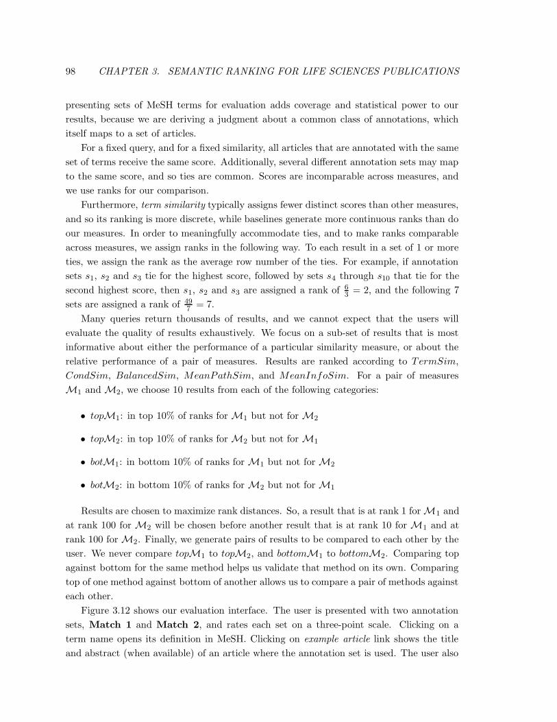
98 CHAPTER 3. SEMANTIC RANKING FOR LIFE SCIENCES PUBLICATIONS
presenting sets of MeSH terms for evaluation adds coverage and statistical power to our
results, because we are deriving a judgment about a common class of annotations, which
itself maps to a set of articles.
For a fixed query, and for a fixed similarity, all articles that are annotated with the same
set of terms receive the same score. Additionally, several different annotation sets may map
to the same score, and so ties are common. Scores are incomparable across measures, and
we use ranks for our comparison.
Furthermore, term similarity typically assigns fewer distinct scores than other measures,
and so its ranking is more discrete, while baselines generate more continuous ranks than do
our measures. In order to meaningfully accommodate ties, and to make ranks comparable
across measures, we assign ranks in the following way. To each result in a set of 1 or more
ties, we assign the rank as the average row number of the ties. For example, if annotation
sets s1, s2 and s3 tie for the highest score, followed by sets s4 through s10 that tie for the
second highest score, then s1, s2 and s3 are assigned a rank of 63 = 2, and the following 7
sets are assigned a rank of 497 = 7.
Many queries return thousands of results, and we cannot expect that the users will
evaluate the quality of results exhaustively. We focus on a sub-set of results that is most
informative about either the performance of a particular similarity measure, or about the
relative performance of a pair of measures. Results are ranked according to TermSim,
CondSim, BalancedSim, MeanPathSim, and MeanInfoSim. For a pair of measures
M1 andM2, we choose 10 results from each of the following categories:
• topM1: in top 10% of ranks forM1 but not for M2
• topM2: in top 10% of ranks forM2 but not for M1
• botM1: in bottom 10% of ranks for M1 but not forM2
• botM2: in bottom 10% of ranks for M2 but not forM1
Results are chosen to maximize rank distances. So, a result that is at rank 1 forM1 and
at rank 100 for M2 will be chosen before another result that is at rank 10 for M1 and at
rank 100 forM2. Finally, we generate pairs of results to be compared to each other by the
user. We never compare topM1 to topM2, and bottomM1 to bottomM2. Comparing top
against bottom for the same method helps us validate that method on its own. Comparing
top of one method against bottom of another allows us to compare a pair of methods against
each other.
Figure 3.12 shows our evaluation interface. The user is presented with two annotation
sets, Match 1 and Match 2, and rates each set on a three-point scale. Clicking on a
term name opens its definition in MeSH. Clicking on example article link shows the title
and abstract (when available) of an article where the annotation set is used. The user also
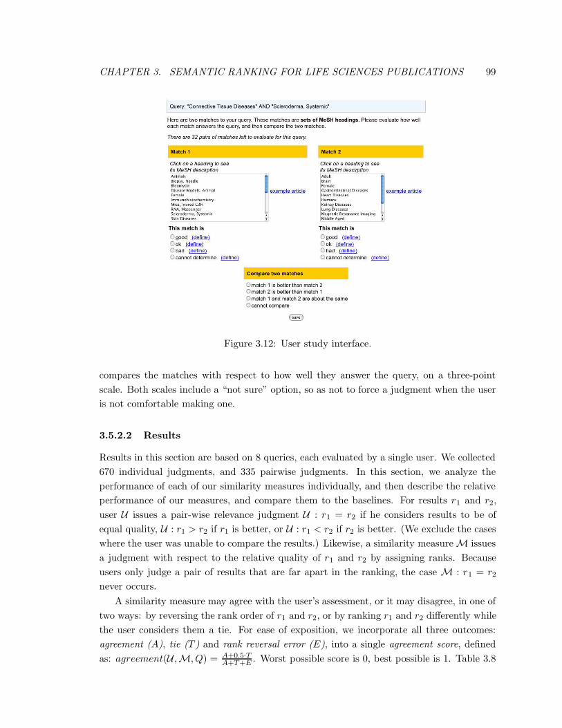
CHAPTER 3. SEMANTIC RANKING FOR LIFE SCIENCES PUBLICATIONS 99
Figure 3.12: User study interface.
compares the matches with respect to how well they answer the query, on a three-point
scale. Both scales include a “not sure” option, so as not to force a judgment when the user
is not comfortable making one.
3.5.2.2 Results
Results in this section are based on 8 queries, each evaluated by a single user. We collected
670 individual judgments, and 335 pairwise judgments. In this section, we analyze the
performance of each of our similarity measures individually, and then describe the relative
performance of our measures, and compare them to the baselines. For results r1 and r2,
user U issues a pair-wise relevance judgment U : r1 = r2 if he considers results to be of
equal quality, U : r1 > r2 if r1 is better, or U : r1 < r2 if r2 is better. (We exclude the cases
where the user was unable to compare the results.) Likewise, a similarity measureM issues
a judgment with respect to the relative quality of r1 and r2 by assigning ranks. Because
users only judge a pair of results that are far apart in the ranking, the case M : r1 = r2
never occurs.
A similarity measure may agree with the user’s assessment, or it may disagree, in one of
two ways: by reversing the rank order of r1 and r2, or by ranking r1 and r2 differently while
the user considers them a tie. For ease of exposition, we incorporate all three outcomes:
agreement (A), tie (T ) and rank reversal error (E), into a single agreement score, defined
as: agreement(U ,M, Q) = A+0.5·TA+T+E
. Worst possible score is 0, best possible is 1. Table 3.8
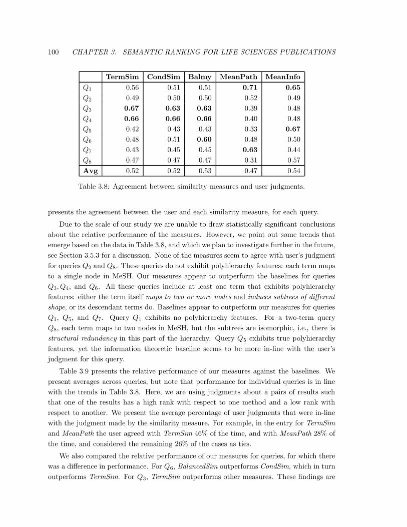
100 CHAPTER 3. SEMANTIC RANKING FOR LIFE SCIENCES PUBLICATIONS
TermSim CondSim Balmy MeanPath MeanInfo
Q1 0.56 0.51 0.51 0.71 0.65
Q2 0.49 0.50 0.50 0.52 0.49
Q3 0.67 0.63 0.63 0.39 0.48
Q4 0.66 0.66 0.66 0.40 0.48
Q5 0.42 0.43 0.43 0.33 0.67
Q6 0.48 0.51 0.60 0.48 0.50
Q7 0.43 0.45 0.45 0.63 0.44
Q8 0.47 0.47 0.47 0.31 0.57
Avg 0.52 0.52 0.53 0.47 0.54
Table 3.8: Agreement between similarity measures and user judgments.
presents the agreement between the user and each similarity measure, for each query.
Due to the scale of our study we are unable to draw statistically significant conclusions
about the relative performance of the measures. However, we point out some trends that
emerge based on the data in Table 3.8, and which we plan to investigate further in the future,
see Section 3.5.3 for a discussion. None of the measures seem to agree with user’s judgment
for queries Q2 and Q8. These queries do not exhibit polyhierarchy features: each term maps
to a single node in MeSH. Our measures appear to outperform the baselines for queries
Q3, Q4, and Q6. All these queries include at least one term that exhibits polyhierarchy
features: either the term itself maps to two or more nodes and induces subtrees of different
shape, or its descendant terms do. Baselines appear to outperform our measures for queries
Q1, Q5, and Q7. Query Q1 exhibits no polyhierarchy features. For a two-term query
Q8, each term maps to two nodes in MeSH, but the subtrees are isomorphic, i.e., there is
structural redundancy in this part of the hierarchy. Query Q5 exhibits true polyhierarchy
features, yet the information theoretic baseline seems to be more in-line with the user’s
judgment for this query.
Table 3.9 presents the relative performance of our measures against the baselines. We
present averages across queries, but note that performance for individual queries is in line
with the trends in Table 3.8. Here, we are using judgments about a pairs of results such
that one of the results has a high rank with respect to one method and a low rank with
respect to another. We present the average percentage of user judgments that were in-line
with the judgment made by the similarity measure. For example, in the entry for TermSim
and MeanPath the user agreed with TermSim 46% of the time, and with MeanPath 28% of
the time, and considered the remaining 26% of the cases as ties.
We also compared the relative performance of our measures for queries, for which there
was a difference in performance. For Q6, BalancedSim outperforms CondSim, which in turn
outperforms TermSim. For Q3, TermSim outperforms other measures. These findings are
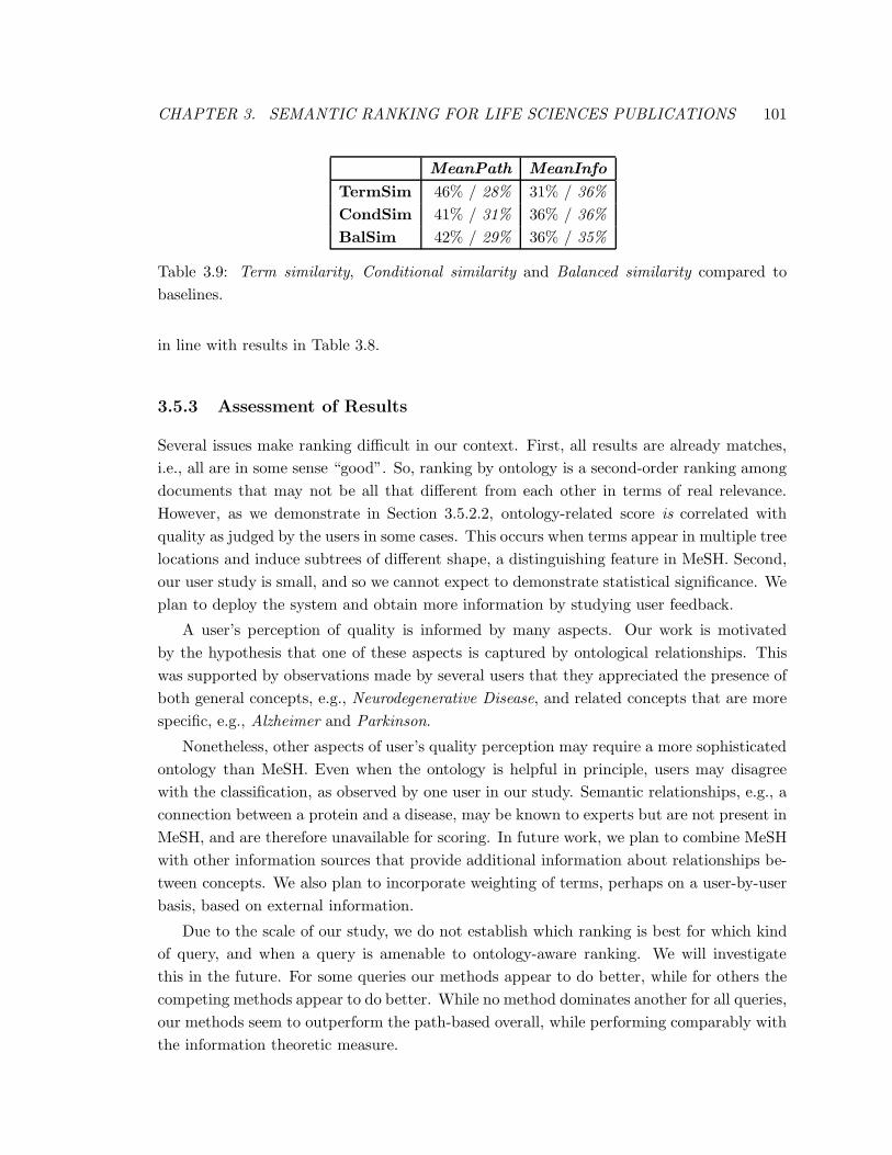
CHAPTER 3. SEMANTIC RANKING FOR LIFE SCIENCES PUBLICATIONS 101
MeanPath MeanInfo
TermSim 46% / 28% 31% / 36%
CondSim 41% / 31% 36% / 36%
BalSim 42% / 29% 36% / 35%
Table 3.9: Term similarity, Conditional similarity and Balanced similarity compared to
baselines.
in line with results in Table 3.8.
3.5.3 Assessment of Results
Several issues make ranking difficult in our context. First, all results are already matches,
i.e., all are in some sense “good”. So, ranking by ontology is a second-order ranking among
documents that may not be all that different from each other in terms of real relevance.
However, as we demonstrate in Section 3.5.2.2, ontology-related score is correlated with
quality as judged by the users in some cases. This occurs when terms appear in multiple tree
locations and induce subtrees of different shape, a distinguishing feature in MeSH. Second,
our user study is small, and so we cannot expect to demonstrate statistical significance. We
plan to deploy the system and obtain more information by studying user feedback.
A user’s perception of quality is informed by many aspects. Our work is motivated
by the hypothesis that one of these aspects is captured by ontological relationships. This
was supported by observations made by several users that they appreciated the presence of
both general concepts, e.g., Neurodegenerative Disease, and related concepts that are more
specific, e.g., Alzheimer and Parkinson.
Nonetheless, other aspects of user’s quality perception may require a more sophisticated
ontology than MeSH. Even when the ontology is helpful in principle, users may disagree
with the classification, as observed by one user in our study. Semantic relationships, e.g., a
connection between a protein and a disease, may be known to experts but are not present in
MeSH, and are therefore unavailable for scoring. In future work, we plan to combine MeSH
with other information sources that provide additional information about relationships be-
tween concepts. We also plan to incorporate weighting of terms, perhaps on a user-by-user
basis, based on external information.
Due to the scale of our study, we do not establish which ranking is best for which kind
of query, and when a query is amenable to ontology-aware ranking. We will investigate
this in the future. For some queries our methods appear to do better, while for others the
competing methods appear to do better. While no method dominates another for all queries,
our methods seem to outperform the path-based overall, while performing comparably with
the information theoretic measure.
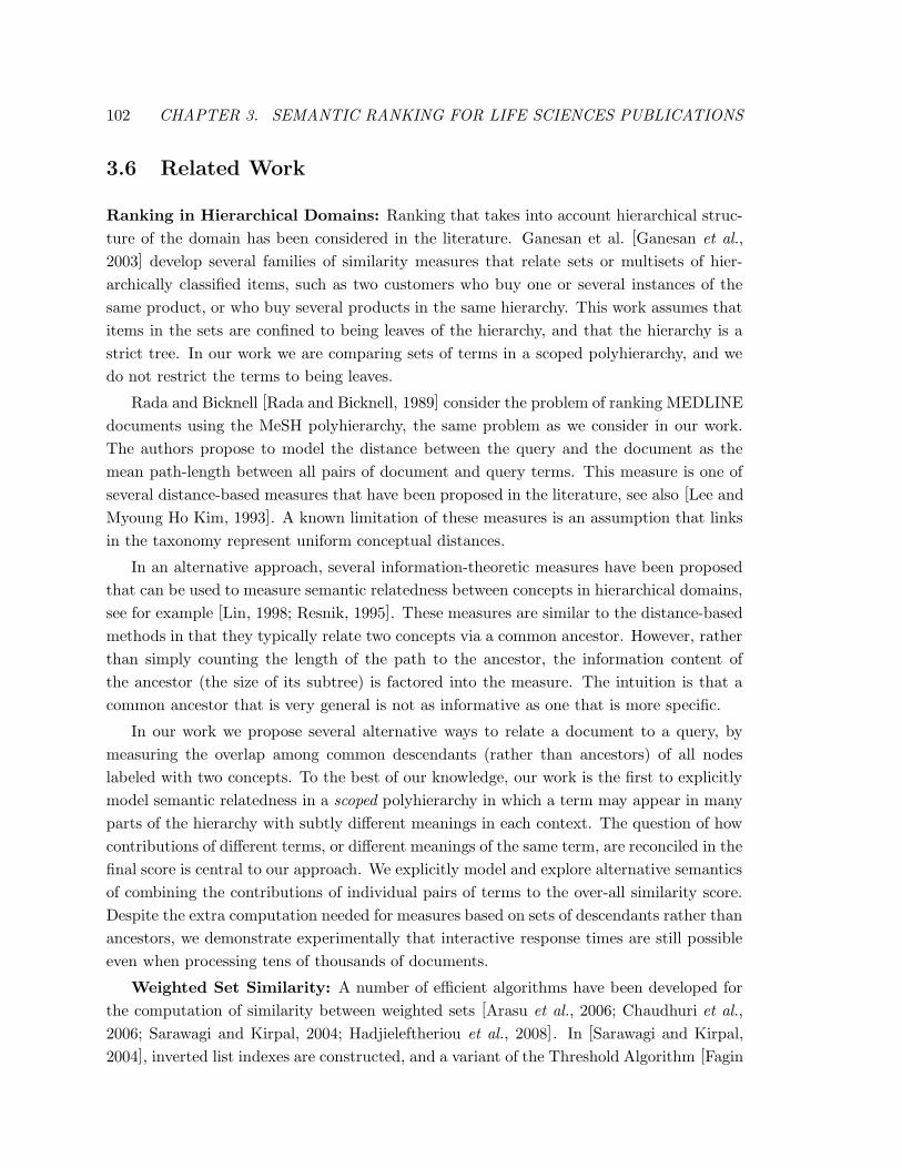
102 CHAPTER 3. SEMANTIC RANKING FOR LIFE SCIENCES PUBLICATIONS
3.6 Related Work
Ranking in Hierarchical Domains: Ranking that takes into account hierarchical struc-
ture of the domain has been considered in the literature. Ganesan et al. [Ganesan et al.,
2003] develop several families of similarity measures that relate sets or multisets of hier-
archically classified items, such as two customers who buy one or several instances of the
same product, or who buy several products in the same hierarchy. This work assumes that
items in the sets are confined to being leaves of the hierarchy, and that the hierarchy is a
strict tree. In our work we are comparing sets of terms in a scoped polyhierarchy, and we
do not restrict the terms to being leaves.
Rada and Bicknell [Rada and Bicknell, 1989] consider the problem of ranking MEDLINE
documents using the MeSH polyhierarchy, the same problem as we consider in our work.
The authors propose to model the distance between the query and the document as the
mean path-length between all pairs of document and query terms. This measure is one of
several distance-based measures that have been proposed in the literature, see also [Lee and
Myoung Ho Kim, 1993]. A known limitation of these measures is an assumption that links
in the taxonomy represent uniform conceptual distances.
In an alternative approach, several information-theoretic measures have been proposed
that can be used to measure semantic relatedness between concepts in hierarchical domains,
see for example [Lin, 1998; Resnik, 1995]. These measures are similar to the distance-based
methods in that they typically relate two concepts via a common ancestor. However, rather
than simply counting the length of the path to the ancestor, the information content of
the ancestor (the size of its subtree) is factored into the measure. The intuition is that a
common ancestor that is very general is not as informative as one that is more specific.
In our work we propose several alternative ways to relate a document to a query, by
measuring the overlap among common descendants (rather than ancestors) of all nodes
labeled with two concepts. To the best of our knowledge, our work is the first to explicitly
model semantic relatedness in a scoped polyhierarchy in which a term may appear in many
parts of the hierarchy with subtly different meanings in each context. The question of how
contributions of different terms, or different meanings of the same term, are reconciled in the
final score is central to our approach. We explicitly model and explore alternative semantics
of combining the contributions of individual pairs of terms to the over-all similarity score.
Despite the extra computation needed for measures based on sets of descendants rather than
ancestors, we demonstrate experimentally that interactive response times are still possible
even when processing tens of thousands of documents.
Weighted Set Similarity: A number of efficient algorithms have been developed for
the computation of similarity between weighted sets [Arasu et al., 2006; Chaudhuri et al.,
2006; Sarawagi and Kirpal, 2004; Hadjieleftheriou et al., 2008]. In [Sarawagi and Kirpal,
2004], inverted list indexes are constructed, and a variant of the Threshold Algorithm [Fagin
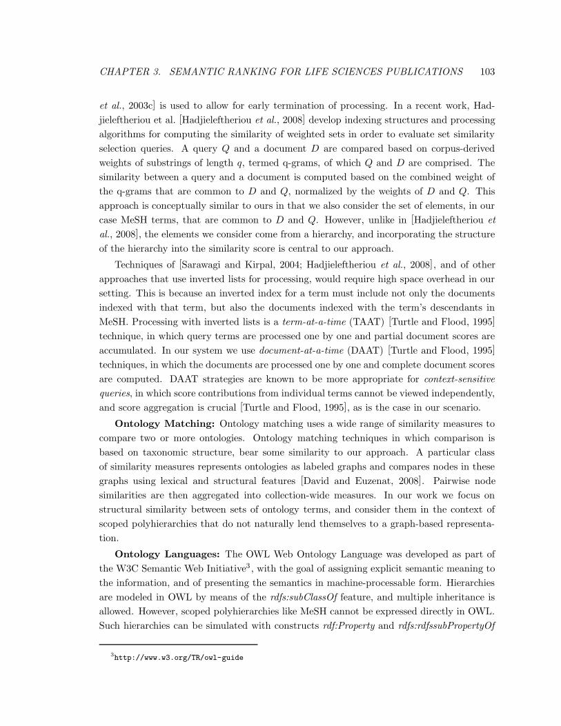
CHAPTER 3. SEMANTIC RANKING FOR LIFE SCIENCES PUBLICATIONS 103
et al., 2003c] is used to allow for early termination of processing. In a recent work, Had-
jieleftheriou et al. [Hadjieleftheriou et al., 2008] develop indexing structures and processing
algorithms for computing the similarity of weighted sets in order to evaluate set similarity
selection queries. A query Q and a document D are compared based on corpus-derived
weights of substrings of length q, termed q-grams, of which Q and D are comprised. The
similarity between a query and a document is computed based on the combined weight of
the q-grams that are common to D and Q, normalized by the weights of D and Q. This
approach is conceptually similar to ours in that we also consider the set of elements, in our
case MeSH terms, that are common to D and Q. However, unlike in [Hadjieleftheriou et
al., 2008], the elements we consider come from a hierarchy, and incorporating the structure
of the hierarchy into the similarity score is central to our approach.
Techniques of [Sarawagi and Kirpal, 2004; Hadjieleftheriou et al., 2008], and of other
approaches that use inverted lists for processing, would require high space overhead in our
setting. This is because an inverted index for a term must include not only the documents
indexed with that term, but also the documents indexed with the term’s descendants in
MeSH. Processing with inverted lists is a term-at-a-time (TAAT) [Turtle and Flood, 1995]
technique, in which query terms are processed one by one and partial document scores are
accumulated. In our system we use document-at-a-time (DAAT) [Turtle and Flood, 1995]
techniques, in which the documents are processed one by one and complete document scores
are computed. DAAT strategies are known to be more appropriate for context-sensitive
queries, in which score contributions from individual terms cannot be viewed independently,
and score aggregation is crucial [Turtle and Flood, 1995], as is the case in our scenario.
Ontology Matching: Ontology matching uses a wide range of similarity measures to
compare two or more ontologies. Ontology matching techniques in which comparison is
based on taxonomic structure, bear some similarity to our approach. A particular class
of similarity measures represents ontologies as labeled graphs and compares nodes in these
graphs using lexical and structural features [David and Euzenat, 2008]. Pairwise node
similarities are then aggregated into collection-wide measures. In our work we focus on
structural similarity between sets of ontology terms, and consider them in the context of
scoped polyhierarchies that do not naturally lend themselves to a graph-based representa-
tion.
Ontology Languages: The OWL Web Ontology Language was developed as part of
the W3C Semantic Web Initiative3 , with the goal of assigning explicit semantic meaning to
the information, and of presenting the semantics in machine-processable form. Hierarchies
are modeled in OWL by means of the rdfs:subClassOf feature, and multiple inheritance is
allowed. However, scoped polyhierarchies like MeSH cannot be expressed directly in OWL.
Such hierarchies can be simulated with constructs rdf:Property and rdfs:rdfssubPropertyOf
3http://www.w3.org/TR/owl-guide
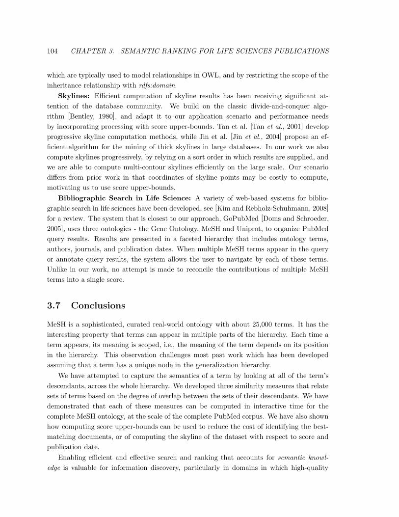
104 CHAPTER 3. SEMANTIC RANKING FOR LIFE SCIENCES PUBLICATIONS
which are typically used to model relationships in OWL, and by restricting the scope of the
inheritance relationship with rdfs:domain.
Skylines: Efficient computation of skyline results has been receiving significant at-
tention of the database community. We build on the classic divide-and-conquer algo-
rithm [Bentley, 1980], and adapt it to our application scenario and performance needs
by incorporating processing with score upper-bounds. Tan et al. [Tan et al., 2001] develop
progressive skyline computation methods, while Jin et al. [Jin et al., 2004] propose an ef-
ficient algorithm for the mining of thick skylines in large databases. In our work we also
compute skylines progressively, by relying on a sort order in which results are supplied, and
we are able to compute multi-contour skylines efficiently on the large scale. Our scenario
differs from prior work in that coordinates of skyline points may be costly to compute,
motivating us to use score upper-bounds.
Bibliographic Search in Life Science: A variety of web-based systems for biblio-
graphic search in life sciences have been developed, see [Kim and Rebholz-Schuhmann, 2008]
for a review. The system that is closest to our approach, GoPubMed [Doms and Schroeder,
2005], uses three ontologies - the Gene Ontology, MeSH and Uniprot, to organize PubMed
query results. Results are presented in a faceted hierarchy that includes ontology terms,
authors, journals, and publication dates. When multiple MeSH terms appear in the query
or annotate query results, the system allows the user to navigate by each of these terms.
Unlike in our work, no attempt is made to reconcile the contributions of multiple MeSH
terms into a single score.
3.7 Conclusions
MeSH is a sophisticated, curated real-world ontology with about 25,000 terms. It has the
interesting property that terms can appear in multiple parts of the hierarchy. Each time a
term appears, its meaning is scoped, i.e., the meaning of the term depends on its position
in the hierarchy. This observation challenges most past work which has been developed
assuming that a term has a unique node in the generalization hierarchy.
We have attempted to capture the semantics of a term by looking at all of the term’s
descendants, across the whole hierarchy. We developed three similarity measures that relate
sets of terms based on the degree of overlap between the sets of their descendants. We have
demonstrated that each of these measures can be computed in interactive time for the
complete MeSH ontology, at the scale of the complete PubMed corpus. We have also shown
how computing score upper-bounds can be used to reduce the cost of identifying the best-
matching documents, or of computing the skyline of the dataset with respect to score and
publication date.
Enabling efficient and effective search and ranking that accounts for semantic knowl-
edge is valuable for information discovery, particularly in domains in which high-quality
CHAPTER 3. SEMANTIC RANKING FOR LIFE SCIENCES PUBLICATIONS 105
ontologies are available. Ontologies represent consensus of the scientific community with
respect to the state of the knowledge in a particular domain. Wide-spread use of ontology-
aware information discovery techniques is valuable not only for the end user, but also for
the evolution of the ontologies: a community of users that sees a benefit in ontology-aware
querying and ranking will keep the ontology up-to-date.
In this chapter we saw how a manually constructed ontology may be used for information
discovery in an annotated document corpus, under the assumption that all documents in
the corpus are of high quality. In the following chapter we will consider how ontologies can
be used for search and ranking over the Wikipedia corpus, where there is a variation in
both quality and relevance.

106 CHAPTER 3. SEMANTIC RANKING FOR LIFE SCIENCES PUBLICATIONS
CHAPTER 4. SEMANTICALLY ENRICHED AUTHORITY PROPAGATION 107
Chapter 4
Semantically Enriched Authority
Propagation
This chapter is based on joint work with Srikanta Bedathur, Klaus Berberich, and Gerhard
Weikum, which appeared in [Stoyanovich et al., 2007].
4.1 Introduction
In Chapter 3 we presented a semantic framework that uses ontology annotations of scientific
publications to rank query results. In the present chapter, we build on the idea of using an
ontology for relevance ranking, and present EntityAuthority: a framework for semantically
enriched authority propagation on graphs that combine documents, entities, and ontological
concepts, in order to improve the ranking of keyword query results.
We apply the techniques of this chapter to Wikipedia, a community-curated encyclope-
dia corpus. Wikipedia may be considered as the middle ground between centrally-curated
digital libraries like PubMed, in which documents are of high quality, and the World Wide
Web, in which there is significant variation in document quality. Like the World Wide Web,
Wikipedia gives rise to a natural link structure, and it is therefore appropriate to apply
link analysis methods in this setting. Like PubMed documents, Wikipedia pages may be
annotated with terms from a ontology, and it is therefore appropriate to use ontology-aware
query processing and raking techniques.
4.1.1 Semantically Enriched Ranking
The classic link analysis methods, such as PageRank [Brin and Page, 1998] and HITS [Klein-
berg, 1999], use the page-level Web graph for authority propagation. These approaches
have been extremely influential. They are, however, fundamentally inappropriate for the
emerging style of semantic Web search that aims to provide users with entities (e.g.,
108 CHAPTER 4. SEMANTICALLY ENRICHED AUTHORITY PROPAGATION
products or scholars) and semantic attributes rather than pages [Cafarella et al., 2007;
Chakrabarti, 2004; Doan et al., 2006a; Chu-Carroll et al., 2006; Hearst, 2006; Madha-
van et al., 2007; Nie et al., 2007]. Recently, techniques have been proposed for analyz-
ing link structure, and for computing rankings of objects in relational databases or in
entity-relationship graphs [Anyanwu et al., 2005; Balmin et al., 2004; Chakrabarti, 2007;
Cheng and Chang, 2007]. However, these methods do not consider Web data or do not
connect the object ranking back to the Web pages where the objects appear. In contrast,
we jointly consider both the page-level and entity-level linkage structures and utilize their
mutual reinforcement for ranking the results of keyword queries against Web data. We
focus on keyword search as this is by far the most common information discovery method
for most users. In our framework we consider two kinds of results: queries can return either
pages or entities.
We utilize information-extraction techniques [Agichtein and Sarawagi, 2006; Cohen et
al., 2003; Cunningham, 2005; Doan et al., 2006b] to identify semantic entities embedded in
the text of Web pages, and to transform the page-level graph into a generalized data graph,
with typed nodes that represent pages or entities, and with typed and weighted edges. We
keep the entity part of this graph as noise-free as possible by mapping entities to nodes
in a richly structured high-quality ontology that describes entities, concepts, and seman-
tic relationships. More specifically, we use the popular open source GATE/ANNIE toolkit
(http://gate.ac.uk/) for named-entity recognition, and various heuristics for entity dis-
ambiguation. According to a recent study that evaluates entity extraction systems [Marrero
et al., 2009], ANNIE supports 12 entity types, and achieves precision and recall in excess
of 70%. While the study finds ANNIE to be inferior to several other systems because it
produces a higher number of false positives, and is sensitive to orthographic features likes
capitalization, this toolkit represented the state of the art at the time when this work was
conducted, and is still among the highest-performing open source systems today.
For the ontology part of our generalized data graph we employ the YAGO knowledge
base, which combines information from the Wikipedia category system and the WordNet
thesaurus into a rigorously structured and highly accurate ontology [Suchanek et al., 2007].
We assume and aim to exploit that there is mutual reinforcement between the authorities
of pages and entities: pages become more valuable if they contain highly authoritative
entities, and entities become more important if they are mentioned by highly authoritative
pages. This resembles the HITS method [Kleinberg, 1999] for Web-graph link analysis and
the ObjectRank method [Balmin et al., 2004], but our approach operates on a generalized
data graph that gives us a much richer substrate for ranking.
Consider for example the query “NBA team”. When issued against a leading search
engine on March 31st, 2007, this query returned links to the official homepage of the Na-
tional Basketball Association, to the NBA-related area of ESPN.com, and to several team
directories. The results were highly relevant but not specific to the user’s information need:
CHAPTER 4. SEMANTICALLY ENRICHED AUTHORITY PROPAGATION 109
it was not apparent from the top-10 results which teams play in the NBA, and there were
no links to any of the teams’ homepages. We observe that super-authorities dominated
the query result, and team homepages did not start appearing until rank 38. (Results
were very similar for the re-phrased query “National Basketball Association team”.) We
consider this and similar queries in our experimental evaluation and demonstrate how our
EntityAuthority ranking methods can benefit such situations.
The results of such queries can be either entities or pages. The former may be preferred
by a skilled user who has the proper context to interpret a concise list of entries such as
“Miami Heat”, “Dallas Mavericks”, and “Chicago Bulls”. The latter is appropriate for a
non-expert user who wants to see an entire textual page, with relevant entities highlighted,
providing him with at-a-glance contextual information. We will show that EntityAuthority
ranking is beneficial for this type of Web-page ranking because it exploits the semantic
connections and mutual authority propagation among pages, entities, and concepts.
4.1.2 Chapter Outline
In the remainder of this chapter we introduce EntityAuthority, and demonstrate its effective-
ness on Wikipedia datasets. Section 4.2 presents the generalized data graph: a semantically-
enriched model of the web graph that maintains information about web pages, and about
the semantic entities that are contained in the pages. In Section 4.3 we describe several
novel authority propagation measures that utilize the structure of the enriched web graph
to a different extent. Section 4.4 details our prototype implementation, and Section 4.5
presents results of our experimental evaluation that demonstrate the effectiveness of our
methods.
4.2 Data Model
In this work, we operate on a directed graph data model that integrates standard Web pages
and their link structure with the entities extracted from these pages and with semantic
relationships among entities. Figure 4.1 illustrates the key components in our data model
using an example based on Web pages related to database research. The data model, which
we call the Generalized Data Graph, or GDG for short, consists of three parts:
• the Enriched Web Graph that is derived using the underlying Web data collection
• the Onto Graph, which represents a richly structured ontological resource
• the Onto Map, a semantic layer that connects the Enriched Web Graph with the Onto
Graph.
We now describe the Generalized Data Graph and its components in greater detail.
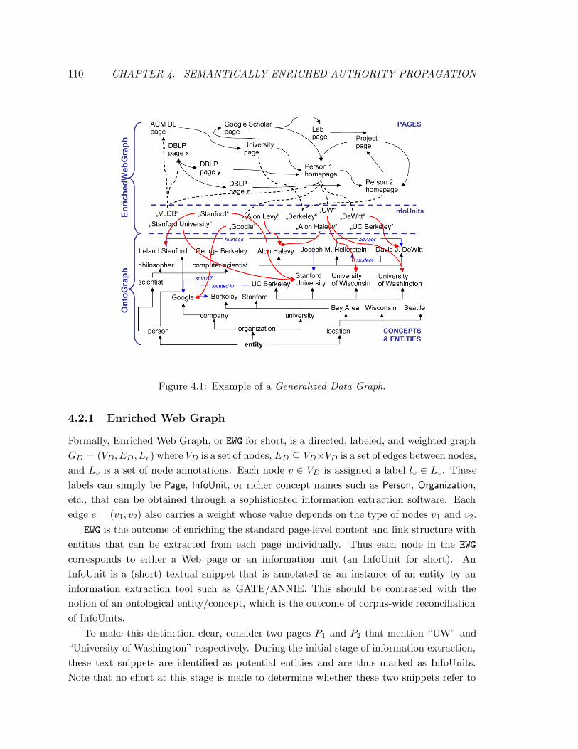
110 CHAPTER 4. SEMANTICALLY ENRICHED AUTHORITY PROPAGATION
Figure 4.1: Example of a Generalized Data Graph.
4.2.1 Enriched Web Graph
Formally, Enriched Web Graph, or EWG for short, is a directed, labeled, and weighted graph
GD = (VD, ED, Lv) where VD is a set of nodes, ED ⊆ VD×VD is a set of edges between nodes,
and Lv is a set of node annotations. Each node v ∈ VD is assigned a label lv ∈ Lv. These
labels can simply be Page, InfoUnit, or richer concept names such as Person, Organization,
etc., that can be obtained through a sophisticated information extraction software. Each
edge e = (v1, v2) also carries a weight whose value depends on the type of nodes v1 and v2.
EWG is the outcome of enriching the standard page-level content and link structure with
entities that can be extracted from each page individually. Thus each node in the EWG
corresponds to either a Web page or an information unit (an InfoUnit for short). An
InfoUnit is a (short) textual snippet that is annotated as an instance of an entity by an
information extraction tool such as GATE/ANNIE. This should be contrasted with the
notion of an ontological entity/concept, which is the outcome of corpus-wide reconciliation
of InfoUnits.
To make this distinction clear, consider two pages P1 and P2 that mention “UW” and
“University of Washington” respectively. During the initial stage of information extraction,
these text snippets are identified as potential entities and are thus marked as InfoUnits.
Note that no effort at this stage is made to determine whether these two snippets refer to
CHAPTER 4. SEMANTICALLY ENRICHED AUTHORITY PROPAGATION 111
the same entity or not.
4.2.2 Onto Graph
We model the underlying ontological resource as a directed, weighted graph GO = (VO, EO, Le)
on a set of nodes VO which correspond to entities/concepts and EO is a multi-set of edges
between these entities. Note that we make no distinction between instances and concepts in
this work. Each edge in EO is annotated with a label from the set of labels, Le that indicates
the relationship between entities connected by the edge. For example, bornIn, locatedIn, and
instanceOf are some of the labels available in YAGO – the precompiled ontology that we
use. Each of these edges is assigned a weight representing the ontology’s confidence in the
relationship.
4.2.3 Onto Map
The next component in our model, Onto Map, forms the layer connecting the InfoUnits
extracted from the corpus with entity and concept nodes in the ontology. Onto Map models
a collection-wide entity reconciliation process that maps InfoUnits onto entities and concepts
of the Onto Graph. This is represented in Figure 4.1 with solid edges from InfoUnits to
Onto Graph layer. In order to support inherent ambiguities in the entity reconciliation
process, our model allows for mapping of a single InfoUnit to more than one concept or
entity. For example, the InfoUnit “UW” is mapped to both “University of Wisconsin” and
“University of Washington”.
4.2.4 Structure of the Generalized Data Graph
The Generalized Data Graph (GDG) that we obtain from extracting entities from pages,
mapping them to the ontology, and connecting entities and concepts by semantic relation-
ships, provides us with a rich cross-reference structure that reflects the authority of both
pages and entities. This graph consists of the following kinds of typed and weighted, di-
rected edges, where all weights are normalized so that the weights of a node’s outgoing
edges sum up to one:
• Hyperlinks between pages normalized by the source page’s out-degree (as in standard
PageRank);
• Edges from a page to each entity or concept that has been extracted from the page,
weighted by the confidence in the extraction and mapping to the corresponding on-
tology node;
• Edges from entities to the concepts to which they belong, weighted with the ontology’s
confidence in the relationship and typed as an isa edge;
112 CHAPTER 4. SEMANTICALLY ENRICHED AUTHORITY PROPAGATION
• Edges from an entity to each of the pages where it appears (i.e., backward pointers
of the information extraction and mapping process), weighted by the extraction and
mapping confidence.
Note that the weights on the edges from entities to pages are not necessarily the same
as those from pages to entities, because of the normalization step: a page may contain only
a few entities, but these entities may appear in many pages.
We do not currently include semantic relationship edges between entities and concepts,
e.g.,bornIn, locatedIn, childOf, etc.
4.2.5 Query Result Graph
In Section 4.3 we will describe how the Generalized Data Graph may be used to compute
authority of various graph nodes. At the high level, authority can reflect either a global
query-independent importance, or it can be made query-dependent. A query-dependent
ranking may be achieved by, for example, first applying a content-only retrieval procedure,
and then ranking over the query-relevant subset of the data.
We now describe a heuristic procedure that constructs a Query Result Graph: a query-
relevant subset of the Generalized Data Graph.
Suppose that we first evaluate a keyword query against both pages and ontology nodes,
and compile a list of qualifying items. We consider an item as qualifying if it contains the
query words or has a compact neighborhood in the data graph that contains them. We will
describe how such a compact neighborhood may be identified in Section 4.4.2.
The resulting items – pages, entities, and concepts, may already carry their initial
relevance scores that reflect frequencies or other kinds of prominence information. We
can now construct a Query Result Graph (QRG for short) from these results, incorporating
relevance scores into node weights.
The QRG consists of all initial results whose relevance score is above some predefined
threshold. This threshold may be set to 0, capturing all qualifying items. Next, for each
item we determine all its predecessors and all its successors in the GDG (these are nodes that
point or are pointed to by the initial results), and we add these nodes to the QRG. We may
then look up all successors of predecessors and all predecessors of successors and add them,
too. How many sets of successors and predecessors will be added can be tuned heuristically.
Having identified a subset of GDG nodes that will be included into the GRG, we now add all
edges from the GDG that connect two QRG nodes. This query-dependent graph construction
is similar to the procedure proposed in the original HITS method [Kleinberg, 1999].
Edge weights can optionally be re-scaled by multiplying the weight of an edge x → y
with the relevance score of the target node y, or with some minimum value µ if y was not
among the initial query results. This is similar to a biased random-walk model in which
a hypothesized Web surfer prefers target nodes whose contents has high relevance scores.
CHAPTER 4. SEMANTICALLY ENRICHED AUTHORITY PROPAGATION 113
Regardless of whether this re-scaling is applied or not, edge weights need to be re-normalized
because not all outgoing edges of a GDG node need be present in the QRG.
4.3 Authority Measures
We now present different models for computing page and entity authority values. The
measures of this section can be applied to the complete Generalized Data Graph, or they
can be applied to the Query Result Graph – a query-specific subset of the GDG.
One immediate candidate for computing a notion of importance on the graph would
be to apply PageRank, or strictly speaking a weighted-edges variant of PageRank [Bharat
and Henzinger, 1998; Borodin et al., 2005] as if all nodes of the graph were pages. But we
will see below that we can apply mathematically related but semantically more meaningful
computations on this richer graph.
The following authority measures can be computed on either the GDG or the QRG. These
measures utilize the rich structure of the graph to a different extent. The first measure
uses only the page nodes of the graphs and then propagates page authority to entities and
concepts; it is thus called Page-Inherited Authority (PIA). The second measure, which is
much more elaborate and one of this chapter’s main contributions, uses the full graph and
is coined Entity-deriVed Authority (EVA).
4.3.1 Page-Inherited Authority
For PIA we consider only the pages in the GDG or the QRG and their incident page-to-page
edges. For each page, we compute either the edge-weighted PageRank or the page authority
according to HITS. Let AP (p) denote the authority of page p, and let P(x) denote the set
of pages that point to ontology node x in the GDG (i.e., the pages from which x has been
extracted). Further, let w(x→ y) denote the weight of the edge from x to y. We define the
page-inherited authority of x as:
AP (x) =∑
p∈P(x)
AP (p)× w(p→ x)
According to PIA, an entity or concept is important if it appears in important pages,
while the importance of a page is pre-determined by a page-links-only authority model.
4.3.2 Entity-Derived Authority
One can argue that importance of a page does not depend solely on the link structure of
the web graph. So, a page may be viewed as important if it mentions important entities
or concepts. This consideration leads to a mutual reinforcement model between pages and
entities. For example, a Web page such as www.cs.stanford.edu is important because
114 CHAPTER 4. SEMANTICALLY ENRICHED AUTHORITY PROPAGATION
it mentions authorities like Jeffrey Ullman and Hector Garcia-Molina, and that these are
in turn authorities because they are referenced by many important Web pages such as
Citeseer-top-authors, DBLP-top-authors, and www.sigmod.acm.org.
To express this intuition we propose an alternative authority propagation model, which
we call Entity deriVed Authority, or EVA. EVA is defined by the following mutually-recursive
equations that define AP – the page-level authority score, and AO – the entity-level author-
ity score:
AP (p) =∑
x∈O(p)
AO(x)× w(x→ p) +∑
q∈P(p)
AP (q)× w(q → p)
AO(x) =∑
p∈P(x)
AP (p)× w(p→ x) +∑
y∈O(x)
AO(y)×w(y → x)
Here, p and q are pages, x and y are entities or concepts, P(z) denotes the set of pages
to which a page, entity, or concept points, and O(z) denotes the set of ontology nodes to
which a page, entity, or concept points.
This model is mathematically related to HITS, where there is mutual reinforcement
between hubs and authorities, but the semantic interpretation of EVA is very different
from HITS. The richer heterogeneous graph structure that we use in EVA also makes the
computation itself more demanding.
The authorities of pages and ontology nodes AP and AO can be iteratively computed by
the Orthogonal Iteration method [Kempe and McSherry, 2004]. In linear algebra notation,
the two equations for AP and AO can be rewritten as follows. Let ~P be a vector of the
pages’ AP values and ~X be a vector of the ontology nodes’ AO values. Suppose there are
m pages and n ontology nodes in the underlying graph. Now let PP be an m×m matrix,
PX an m× n matrix, XP an n×m matrix, and XX and n× n matrix with the following
entries:
PPij = w(i→ j) for pages i, j with i 6= j
= 0 for i = j
PXij = w(i→ j) for page i and ontology node j
XPij = w(i→ j) for ontology node i and page j
XXij = w(i→ j) for ontology nodes i, j with i 6= j
= 0 for i = j
Then the equations for AP and AO given above can be phrased in vector form as:
~P = XP × ~X + PP × ~P (4.1)
CHAPTER 4. SEMANTICALLY ENRICHED AUTHORITY PROPAGATION 115
~X = PX × ~P + XX × ~X (4.2)
The computation is initialized by choosing arbitrary start vectors for P and X that are
not linearly dependent on the eigenvectors of the matrices in Equations 4.1 and 4.2. It is
not difficult to satisfy this start condition; for example, it is satisfied by choosing uniform
start values in all but degenerate situations. Then we evaluate each of the two equations by
substituting the current values of the two vectors in their right-hand side; the new values
for the left-hand side then become the values for the right-hand side of the next iteration.
Iteration repeats until the changes of the two vectors, as reflected either by their L1 norms,
or by the relative ranking of their top-100 elements, drop below some threshold and become
negligible. After each iteration step, the two vectors are re-scaled (i.e., multiplied by a
normalization factor) so that their L1 norms become equal to one. This final step ensures
convergence and result uniqueness for the Orthogonal Iteration method.
4.3.3 Untyped Authority
The PIA model computes a global authority score of an entity based on global authority
of the page(s) from which the entity was extracted. In contrast, EVA models mutual
reinforcement between pages and entities on the graph.
For completeness we also present a third ranking method, which we call Un-Typed Au-
thority, or UTA. UTA serves as the middle-ground between PIA and EVA. Like EVA, UTA
will operate over all nodes and edges of the GDG, or over the query specific QRG. However,
unlike EVA, UTA simply runs an edge-weighted version of a standard ranking algorithm
(e.g. PageRank or HITS) on this graph, ignoring node types.
We will compare the effectiveness of PIA, UTA, and EVA in Section 4.5.
4.4 System Implementation
This section describes the system architecture of our prototype implementation. Our pro-
totype was evaluated on a part of the English-language Wikipedia.
4.4.1 Building the Generalized Data Graph
We use several existing tools to build the Generalized Data Graph, and while information
annotation and extraction is not a major contribution of this work, we gained some insight
into performing these tasks on a fairly large scale. We used the GATE/ANNIE toolkit to
identify entities of types Location, Person and Organization in the corpus, and were able
to automatically extract over 1.2 million annotations as InfoUnits. Entity annotation was
time-consuming, forcing us to limit our experimental evaluation to a relatively small corpus.
116 CHAPTER 4. SEMANTICALLY ENRICHED AUTHORITY PROPAGATION
However, while extraction may be a bottleneck in an academic setting, this process can be
parallelized, and can be done on a large scale if enough hardware is available.
As the next step we group together InfoUnits that refer to the same real-life entity. For
example, we would unify two occurrences of the same string (e.g. “Michael Jordan”) into
a single entity. We also attempt to identify InfoUnits that do not match literally, but are
nonetheless likely to refer to the same real-life entity, e.g. “Michael Jordan” and “Mike
Jordan”. We rely on a combination of heuristics to identify groups of InfoUnits with high
degree of string similarity. We consider strings that are at least 4 characters in length, and
that match according to the SecondString[Cohen et al., 2003] JaroWinkler-TFIDF metric,
with a similarity of at least 0.95 out of 1.0. Additionally, we use the highly-accurate means
relationship in YAGO [Suchanek et al., 2007] to identify pairs of synonymous strings. Using
these simple and efficient heuristics we map 1.2 million InfoUnits to 240 thousand entities.
Finally, we use the same string-based heuristics to map discovered entities to nodes in
YAGO. If an entity maps to one or several nodes in the ontology, we add the appropriate
mapping edges to the GDG (these are the solid arrows from InfoUnits to ontology nodes in
Figure 4.1). If no node in the Onto Graph is identified as a target for mapping, we add
discovered entities to the OntoGraph, placing them directly under Person, Organization or
Location.
During the initial stages of this project, we considered more sophisticated (and less
restrictive) ways of grouping together similar InfoUnits and of mapping such groups to on-
tology nodes. We eventually found that these techniques introduced a considerable amount
of noise, causing topic drift. We conclude that more sophisticated context-aware tools are
required to reliably match strings that do not pass the 0.95 similarity threshold. Using such
tools (once they become available and are efficient enough to operate on the large scale)
would benefit our method.
4.4.2 Query Processing
Our system processes keyword queries, and returns both pages and entities as query results.
In this work we focus primarily on the construction of the data graph and on ranking,
not on query processing, and we use a simple query processing method in our prototype
implementation.
We store the Generalized Data Graph in an Oracle 10g RDBMS, and use Oracle Text
to identify relevant pages and entities at query time. Matches are identified using a tf-
idf-based algorithm that incorporates stemming and word proximity information. Relevant
entries receive a non-zero relevance score from Oracle, and we normalize this score to the
(0, 1] range.
A page is considered relevant to a query if its body contains all words present in the
query. The final score of a page is the product of its authority and relevance scores.
CHAPTER 4. SEMANTICALLY ENRICHED AUTHORITY PROPAGATION 117
We identify entities that are relevant to a query using the OntoGraph built from YAGO.
An entity is considered relevant to a query if at least one of the following conditions is met:
• The entity matches the query by name;
• The entity has strong string similarity with an ontology node that matches the query;
• The thematic neighborhood of the entity matches the query. Thematic neighborhoods
are formed by combining all parents of an entity or concept, i.e. by following is-a and
instance-of ontology edges.
Consider for example the Serbian basketball player Vlade Divac. YAGO assigns Vlade
to several categories, including Serbian basketball players, LA Lakers players, and Olympic
competitors for Yugoslavia. Vlade’s thematic neighborhood includes all these category
names. For this reason the entity Vlade Divac will be returned as a match for queries
like ”Serbian LA Lakers players” and ”Olympic basketball competitors”. Relevant entities
are ranked according to their authority scores; the relevance score of the query with respect
to the thematic neighborhood is discarded.
The identified relevant pages and entities are added to the Query Result Graph. The
graph is then expanded by including predecessors and successors. The entire QRG is used
for ranking, but only the relevant pages and entities are returned as the query result.
4.5 Experimental Evaluation
4.5.1 Experimental Setup
We evaluate the performance of our system on a subset of the English-language Wikipedia;
we focus on two thematic slices: Serbia and basketball. Pages were included into the respec-
tive slice based on whether they contain the words “Serbia” and “basketball”. The slices
are comparable in size, and together include about 7800 Wikipedia articles.
We selected 20 keyword queries, 10 queries per slice, for our experimental evaluation.
Queries ranged between 1 and 6 words in length. Some examples of queries are lake,
politician, physics, living writer prize winner on the Serbia slice, and NBA venue, college
basketball, African American basketball player Olympic competitor on the basketball slice.
Queries were selected so as to have non-trivial recall in the ontology with respect to the
slice: query terms had to match thematic neighborhoods of at least a few ontology nodes
relevant to the slice. We allowed for significant variation in ontology recall: for some queries,
hundreds of ontology nodes matched, while for others there were only a handful of matches.
In the most extreme case, only one ontology node matched the query.
We compare four ranking methods in our experiments: one query-independent and three
that re-rank results at query time. These are query-independent PageRank (PR) for pages,
118 CHAPTER 4. SEMANTICALLY ENRICHED AUTHORITY PROPAGATION
and the corresponding Page-Inherited Authority (PIA) for entities. Query-time re-ranking
methods include Un-Typed Authority with PageRank (UTA-PR) and with HITS (UTA-
HITS), and Entity-Derived Authority (EVA). We consider top-20 pages and top-20 entities
returned by each ranking method in our evaluation.
For a given query, top-ranking results were collected and pooled. The quality of each re-
sult was then evaluated by two of the co-authors of this work. Evaluators had no knowledge
either of the method that retrieved the result, or of the result’s rank. We used a simple
goodness metric, a value between 0 and 2, in our evaluation, and averaged the goodness
scores if there was disagreement. Goodness scores were assigned as follows: 0 for irrelevant,
1 for somewhat relevant or relevant but not very important, and 2 for very relevant. To
judge goodness of an entity, the evaluator was asked to identify a Wikipedia page that was
most relevant to the entity, and use the contents of the page to guide the evaluation. We
also considered using a combination of metrics, such as coverage and specificity, to evaluate
the results. However, these metrics were designed with documents (or parts of documents)
in mind, and it was not clear how to apply them to entities and concepts.
We use four metrics to assess the performance of the ranking methods: discounted
cumulated gain (DCG) [Jarvelin and Kekalainen, 2002], normalized discounted cumulated
gain (NDCG) [Jarvelin and Kekalainen, 2002], precision, and recall. All metrics were applied
at top-20. DCG and NDCG are described in detail in Section 1.1.3.2. Recall that DCG is
a cumulative metric that weighs goodness scores by rank, penalizing entries that appear at
later ranks. NDCG is an average metric that normalizes each entry in the DCG vector by
the corresponding value in the ideal vector. We report DCG in addition to NDCG because
it incorporates recall (a low-recall method may have a perfect NDCG score, but it will not
have a perfect DCG score). As suggested in [Jarvelin and Kekalainen, 2002], we use b = 2
as the discount factor. For recall, we consider an entry to be relevant to a query if at least
one of the two evaluators considered the entry relevant (goodness score ≥ 0.5). Precision
is calculated with respect to the ideal: we pool together the relevant entries retrieved by
all methods, order them by descending goodness scores, and calculate recall at top-20.
Precision of a ranking method is then calculated as recallmethod/recallideal.
4.5.2 Results and Discussion
Results of our experimental evaluation are summarized in Tables 4.1 and 4.2. All methods
that involve query-time re-ranking operate on the Query Result Graph: a query-dependent
subset of the Generalized Data Graph. Each entry represents an average among 20 queries
in our experiments. We view results obtained by query-independent PageRank (PR entry
in Table 4.2) as the base-line for our experiments. Note that NDCG, precision, and recall
are normalized, and that perfect DCG is 15.63 in our setting.
We make the following observations from these results.
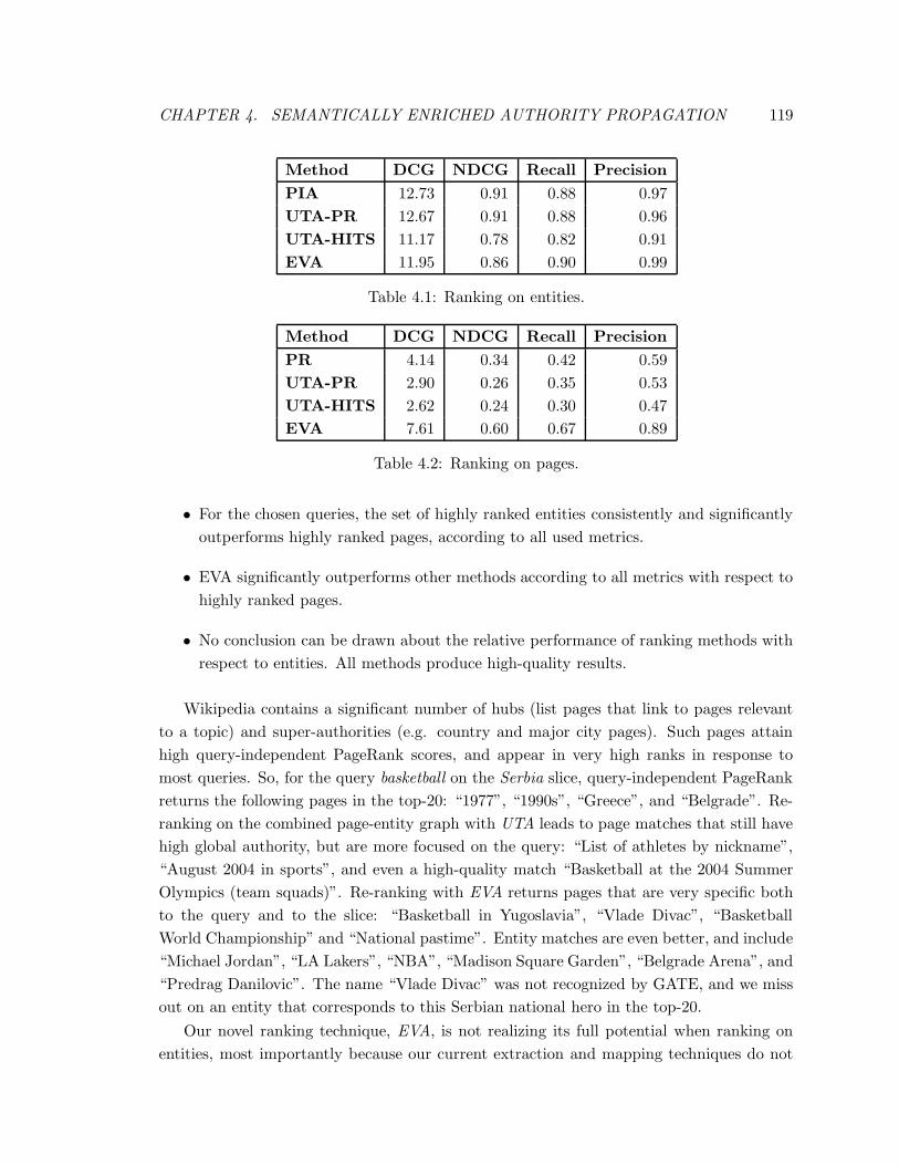
CHAPTER 4. SEMANTICALLY ENRICHED AUTHORITY PROPAGATION 119
Method DCG NDCG Recall Precision
PIA 12.73 0.91 0.88 0.97
UTA-PR 12.67 0.91 0.88 0.96
UTA-HITS 11.17 0.78 0.82 0.91
EVA 11.95 0.86 0.90 0.99
Table 4.1: Ranking on entities.
Method DCG NDCG Recall Precision
PR 4.14 0.34 0.42 0.59
UTA-PR 2.90 0.26 0.35 0.53
UTA-HITS 2.62 0.24 0.30 0.47
EVA 7.61 0.60 0.67 0.89
Table 4.2: Ranking on pages.
• For the chosen queries, the set of highly ranked entities consistently and significantly
outperforms highly ranked pages, according to all used metrics.
• EVA significantly outperforms other methods according to all metrics with respect to
highly ranked pages.
• No conclusion can be drawn about the relative performance of ranking methods with
respect to entities. All methods produce high-quality results.
Wikipedia contains a significant number of hubs (list pages that link to pages relevant
to a topic) and super-authorities (e.g. country and major city pages). Such pages attain
high query-independent PageRank scores, and appear in very high ranks in response to
most queries. So, for the query basketball on the Serbia slice, query-independent PageRank
returns the following pages in the top-20: “1977”, “1990s”, “Greece”, and “Belgrade”. Re-
ranking on the combined page-entity graph with UTA leads to page matches that still have
high global authority, but are more focused on the query: “List of athletes by nickname”,
“August 2004 in sports”, and even a high-quality match “Basketball at the 2004 Summer
Olympics (team squads)”. Re-ranking with EVA returns pages that are very specific both
to the query and to the slice: “Basketball in Yugoslavia”, “Vlade Divac”, “Basketball
World Championship” and “National pastime”. Entity matches are even better, and include
“Michael Jordan”, “LA Lakers”, “NBA”, “Madison Square Garden”, “Belgrade Arena”, and
“Predrag Danilovic”. The name “Vlade Divac” was not recognized by GATE, and we miss
out on an entity that corresponds to this Serbian national hero in the top-20.
Our novel ranking technique, EVA, is not realizing its full potential when ranking on
entities, most importantly because our current extraction and mapping techniques do not
120 CHAPTER 4. SEMANTICALLY ENRICHED AUTHORITY PROPAGATION
allow us to include inter-entity edges into the QRG, limiting the flow of authority, particularly
for entities.
The choice of relatively small thematic slices for our experiments makes the size of the
Generalized Web Graph more manageable, but confines us to working with only a small
subset of the ontology, limiting the recall of entity-based methods in some cases. For
example, the query “orthodox monastery” on the Serbia slice was able to identify a single
entity as a match – the monastery Hilandar. This happened because the ontology contained
a limited amount of information relevant both to the query and to the thematic slice. The
situation was further aggravated by the fact that the GATE/ANNIE Toolkit was not very
successful when mining foreign-language names, and so many InfoUnits that could have
been matched to relevant Onto Graph nodes went unnoticed.
4.6 Related Work
Link Analysis: Link analysis has come a long way since the seminal articles by Klein-
berg [Kleinberg, 1999] and Page et al. [Page et al., 1998] were published. These early
approaches and their extensions, overviews of which are given in [Borodin et al., 2005;
Langville and Meyer, 2004], are based on a simple directed graph model. More sophisti-
cated (e.g., weighted, multi-type, and labeled) graph models were considered in [Bhalo-
tia et al., 2002; Chitrapura and Kashyap, 2004; Geerts et al., 2004; Guo et al., 2003;
Xi et al., 2004]. More recently, the paradigm of link analysis has been carried over to graphs
other than the Web graph, namely, relational databases with records and foreign-key re-
lationships constituting the nodes and edges of the graph, and entity-relationship graphs
that capture, for example, bibliographic data such as DBLP or Citeseer. Such settings have
led to new forms of ObjectRank, PopRank, or EntityRank measures [Anyanwu et al., 2005;
Balmin et al., 2004; Chakrabarti, 2007; Cheng and Chang, 2007; Nie et al., 2005]. Objec-
tRank [Balmin et al., 2004] resembles our approach because it is also inspired by HITS, but
it does not address Web data at all. EntityRank [Cheng and Chang, 2007] addresses the
ranking of entities extracted from Web pages, but its focus is on frequency-based content
strength and it does not consider the graph structure of the Web and its embedded entities.
PopRank [Nie et al., 2005] is closest to our framework; it uses a “random object finder”
model on an object-relationship graph and combines this with a prior popularity derived
from pages’ PageRank values (the latter is similar to our PIA method). Our approach is
more powerful because we treat both pages and entities as first-class citizens in ranking,
and because we also consider ontological relationships and confidence values from extraction
and disambiguation.
Entity Search: Searching the Web at the finer and semantically more expressive
granularity of entities (Web objects) and their relationships, instead of the coarser page
granularity prevalent today, has been pursued in different variants like faceted search,
CHAPTER 4. SEMANTICALLY ENRICHED AUTHORITY PROPAGATION 121
vertical search, object search, and entity-relationship search (e.g., [Chakrabarti, 2004;
Chang, 2006; Doan et al., 2006a; Hearst, 2006; Madhavan et al., 2007; Nie et al., 2005].
The approaches most closely related to our work are the Libra system [Nie et al., 2007;
Nie et al., 2005], the EntitySearch engine [Cheng and Chang, 2007], and the ExDB system
[Cafarella et al., 2007]. All three systems extract entities and relations from Web data
and provide ranked retrieval. Libra uses a variety of techniques for ranking, including the
PopRank model mentioned above and a record-level statistical language model; the Enti-
tySearch engine mostly relies on occurrence-frequency statistics; ExDB factors extraction
confidence values into its ranking but does not consider any link information. None of these
ranking models considers the mutual authority propagation between entities and pages that
we exploit in our Generalized Data Graph.
4.7 Conclusions
In this chapter we developed an entity-aware ranking framework, and presented a novel
ranking algorithm, EntityAuthority, that models the mutual reinforcement between pages
and entities. We demonstrated how an ontology can be used for query processing and
ranking in this setting. We presented a prototype implementation of our system, and
experimentally demonstrated the improvement in query result quality.
EntityAuthority is an example of a search and ranking framework that can be used in
a heterogeneous setting, where relevance and quality of a result is determined based on
ontological relationships, link structure of page graph, etc. Techniques of this chapter may
be combined with the similarity measures of Chapter 3, making the ontology-based portion
of the ranking more sophisticated in presence of a scoped polyhierarchy. For example, an
iterative authority propagation mechanism may be developed for PubMed, in which scores
of documents would be initialized with similarity scores of Chapter 3, and documents and
MeSH terms would then be re-ranked with EntityAuthority. Such re-ranking would operate
over a linked graph of documents, with semantics of the links capturing the semantics of
quality, or authority. For example, links between documents may be established based on
co-authorship, citations, publication venues, or authors’ affiliations.

122 CHAPTER 4. SEMANTICALLY ENRICHED AUTHORITY PROPAGATION
CHAPTER 5. RANK-AWARE CLUSTERING OF STRUCTURED DATASETS 123
Chapter 5
Rank-Aware Clustering of
Structured Datasets
This chapter presents joint work with Sihem Amer-Yahia [Stoyanovich and Amer-Yahia,
2009]. We would like to thank Duncan Watts and Jake Hofman for their help and valuable
discussions.
5.1 Introduction
In Chapter 2 we explored how semantics of social connections may be used for information
discovery. In Chapters 3 and 4 we considered how semantics of an ontology may be used for
search and ranking. In the present chapter we explore how semantic relationships among
item attributes may be used for rank-aware information discovery.
In online applications that involve large structured datasets, such as Yahoo! Personals
and Trulia.com, there are often thousands of high-quality items, in this case, persons and
apartments, that satisfy a user’s information need. Users typically specify a structured
target profile in the form of attribute-value pairs, and this profile is then used by the
system to filter items. On dating sites, a target profile may specify the age, height, income,
education, political affiliation, and religion of a potential match. In real estate applications,
a profile describes a user’s dream home by its location, size, and number of bedrooms.
The number of matches to a specific profile is often very high, making data exploration an
interesting challenge.
Typically users also specify ranking criteria that are used to rank matches. For example,
in Yahoo! Personals, potential matches can be ranked by decreasing income or increasing
age, while in Trulia.com, available houses may be ranked by increasing price or decreasing
size. Ranking helps users navigate the set of results by limiting the number of items that
they see at any one time, and by making sure that the items users see first are of high
quality (according to the ranking criteria). However, ranking also brings the disadvantage
124 CHAPTER 5. RANK-AWARE CLUSTERING OF STRUCTURED DATASETS
of match homogeneity: the user is often required to go through a large number of similar
items before finding the next different item. This is illustrated in the following fictional
example inspired by Yahoo! Personals.
Example 5.1.1 User Mike is looking for a date. Mike specifies that he is interested in
women who are 20 to 30 years old and who have some college education, and requests that
results be sorted on income in descending order. When inspecting the results, Mike notices
that the top ranks are dominated by women in their late-twenties with a Master’s degree. It
takes Mike a while to scroll down to the next set of matches that are different from the top-
ranking ones. In doing so, he skips over some unexpected cases such as younger women with
higher education and income levels, or women with high income who did not graduate from
college. After additional data exploration, Mike realizes that there is a correlation between
age, education (filtering), and income (ranking). Such correlations would have been obvious
if data were presented in labeled groups such as [20-24] year-olds with a bachelor’s
degree, [25-30] year-olds who make more than 75K, etc.
A key point that arises from this example is that a user who is browsing a result set
sequentially, item by item, is only able to infer some trends and correlations in the data after
seeing a significant number of items. Sequential presentation is not very helpful if the user
is trying to understand general properties of a dataset, i.e., explore the data, particularly
if the dataset is large.
The complexity of manual data exploration increases with more sophisticated ranking.
For example, Mike’s profile could provide a custom scoring function that computes a score
which is inversely proportional to the distance from his geographic location to the location
of his match, and directly proportional to the match’s income. Helping the users better
understand the results, which enables easier navigation and profile refinement, is even more
important in this case, given that correlations between item attributes and the ranking
function are less obvious.
5.1.1 Motivating User Study
In order to better understand the challenges of ranked data exploration, we interviewed
six potential users. All users were male, and they were all members of Yahoo! Research.
Users were asked to specify a realistic Yahoo! Personals profile, and to discuss their data
exploration experience with us during the course of the interview. We conducted free-form
interviews and did not use a questionnaire so as not to influence the users’ statements by a
limited menu of options. Users were allowed to select among a pre-specified set of ranking
attributes.
User profiles were evaluated by our prototype implementation, against the Yahoo! Per-
sonals dataset. Profile matches were presented in two ways: ranked list and clustered items.
CHAPTER 5. RANK-AWARE CLUSTERING OF STRUCTURED DATASETS 125
Three users were shown the ranked list first, followed by clustered items; the order was
reversed for the other three users.
As the users were interacting with the ranked list interface, they noted that results are
homogeneous: there was little variation in attribute values among top-ranked items. As a
result, item attributes were ignored by most users, and the decision of whether to further
explore a particular profile was based solely on the photo. All six users explicitly stated
result homogeneity as a concern. The other key observation was that ranking is opaque.
Indeed, item ordering was not considered helpful in data exploration and was not well-
understood by some users. Even for single-attribute ranking, some users wanted to see
items with a variety of values for the ranking attribute. Two users explicitly stated this
limitation.
During their interaction with the clustered items interface users noted that diverse re-
sults were more easily accessible, and that clustered items helped them refine their search
preferences. Three out of six users decided to refine their query moments after seeing clus-
ters of results. Two of the three explicitly commented that the presentation enabled them
to quickly understand the result set and to refine their query more effectively.
5.1.2 Limitations of Clustering Algorithms
Clustering is an effective data exploration method that is applicable to structured, semistruc-
tured, and unstructured data alike. Clustering algorithms assign N items to K � N groups,
where K is either known in advance or discovered by the algorithm. To be useful for data
exploration, the algorithm must produce meaningful descriptions for the clusters. There
are many families of clustering algorithms that can be used for this task. Some algorithms
partition the dataset, while others assign each point to zero, one, or several clusters. Some
algorithms operate over all item attributes, while others attempt dimensionality reduction
techniques. In domains like Yahoo! Personals, where datasets are large and all items are
described by a large number of attributes, it is intuitive to use subspace clustering.
Subspace clustering is an extension of traditional clustering that seeks to find clusters
in different subspaces of a dataset [Parsons et al., 2004]. Clusters of items are high-quality
regions identified in multiple, possibly overlapping, subspaces. Many subspace clustering
algorithms use the density of a region as a quality measure. In the simplest case, density is a
percentage of data points that fall within a particular region, and the algorithm aims to find
all regions that have density higher than a pre-defined threshold. We give an overview of one
of the first subspace clustering algorithms, CLIQUE [Agrawal et al., 1998], in Section 5.3.1,
and we illustrate it here with an example.
Example 5.1.2 Consider a fictional real estate example in Table 5.1: a database of 300
rental apartments, listing the number of bedrooms, number of bathrooms, size in ft2, monthly
rental price, and the number of such apartments currently on the market. Mary is looking
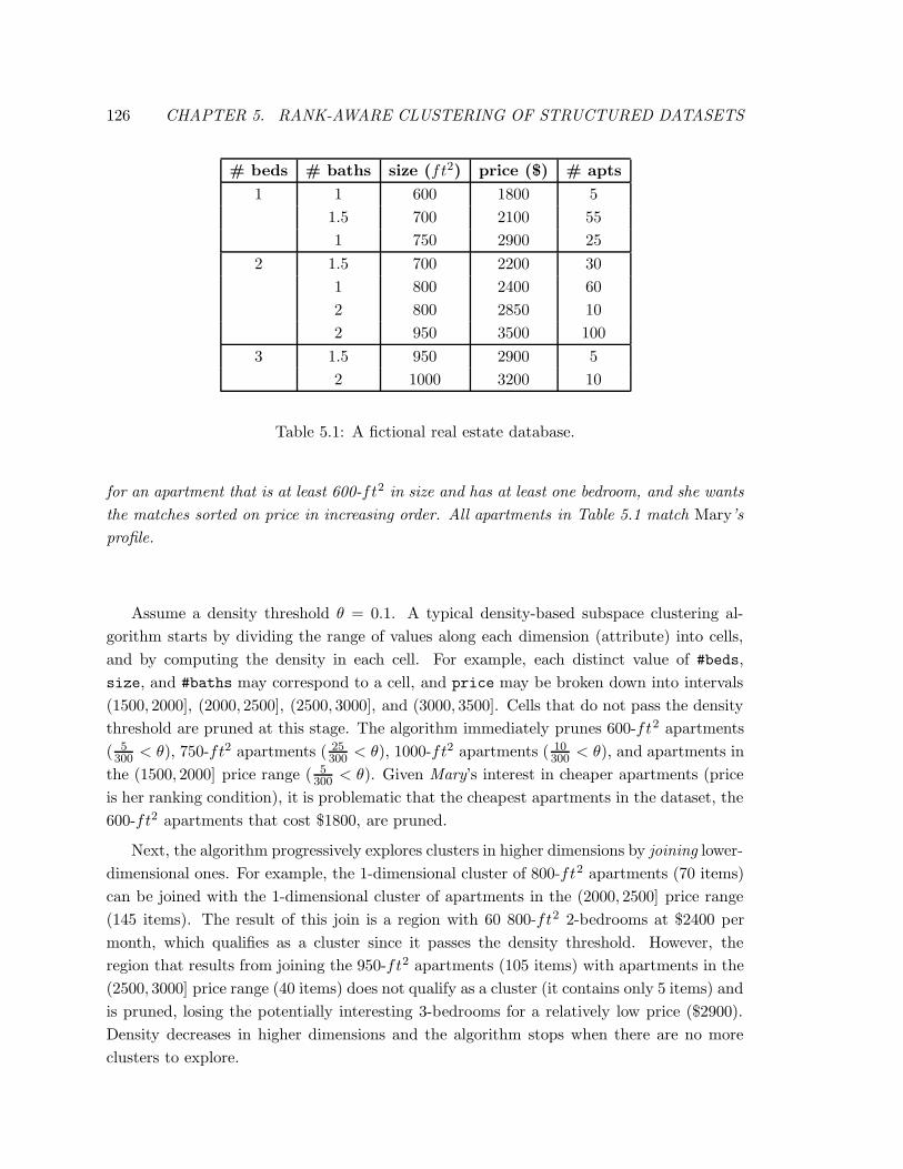
126 CHAPTER 5. RANK-AWARE CLUSTERING OF STRUCTURED DATASETS
# beds # baths size (ft2) price ($) # apts
1 1 600 1800 5
1.5 700 2100 55
1 750 2900 25
2 1.5 700 2200 30
1 800 2400 60
2 800 2850 10
2 950 3500 100
3 1.5 950 2900 5
2 1000 3200 10
Table 5.1: A fictional real estate database.
for an apartment that is at least 600-ft2 in size and has at least one bedroom, and she wants
the matches sorted on price in increasing order. All apartments in Table 5.1 match Mary’s
profile.
Assume a density threshold θ = 0.1. A typical density-based subspace clustering al-
gorithm starts by dividing the range of values along each dimension (attribute) into cells,
and by computing the density in each cell. For example, each distinct value of #beds,
size, and #baths may correspond to a cell, and price may be broken down into intervals
(1500, 2000], (2000, 2500], (2500, 3000], and (3000, 3500]. Cells that do not pass the density
threshold are pruned at this stage. The algorithm immediately prunes 600-ft2 apartments
( 5300 < θ), 750-ft2 apartments ( 25
300 < θ), 1000-ft2 apartments ( 10300 < θ), and apartments in
the (1500, 2000] price range ( 5300 < θ). Given Mary’s interest in cheaper apartments (price
is her ranking condition), it is problematic that the cheapest apartments in the dataset, the
600-ft2 apartments that cost $1800, are pruned.
Next, the algorithm progressively explores clusters in higher dimensions by joining lower-
dimensional ones. For example, the 1-dimensional cluster of 800-ft2 apartments (70 items)
can be joined with the 1-dimensional cluster of apartments in the (2000, 2500] price range
(145 items). The result of this join is a region with 60 800-ft2 2-bedrooms at $2400 per
month, which qualifies as a cluster since it passes the density threshold. However, the
region that results from joining the 950-ft2 apartments (105 items) with apartments in the
(2500, 3000] price range (40 items) does not qualify as a cluster (it contains only 5 items) and
is pruned, losing the potentially interesting 3-bedrooms for a relatively low price ($2900).
Density decreases in higher dimensions and the algorithm stops when there are no more
clusters to explore.
CHAPTER 5. RANK-AWARE CLUSTERING OF STRUCTURED DATASETS 127
5.1.3 Challenges of Rank-Aware Clustering
A lower density threshold would evidently guarantee that some of the regions pruned using
a higher threshold would be preserved. However, if the threshold is set too low, the al-
gorithm would keep merging neighboring cells, ultimately identifying much larger clusters,
and possibly one cluster containing the entire dataset. Moreover, not all regions that pass a
typical clustering quality metric, e.g., density or entropy, are equally interesting to the user.
Indeed, given a scoring function, some items, and hence some clusters, are more desirable
than others (e.g., Mary has little interest in the 2-bedroom apartments that cost $3500, but
would like to see the 1-bedrooms that cost $1800). Even when the density of a region is
high, as is the case with 2-bedroom apartments for $3500, Mary would probably have less
interest in them than in cheaper apartments. Therefore, we propose to explore rank-aware
clustering quality measures which account for item scores and ranks in assessing cluster
quality.
5.1.4 Chapter Outline
In the remainder of this chapter we present BARAC: a Bottom-up Algorithm for Rank-
Aware Clustering of structured datasets. We start by formalizing new clustering quality
measures for rank-aware data exploration in Section 5.2, and develop an adaptation of a
bottom-up APRIORI-style subspace clustering algorithm for this setting in Section 5.3. In
Section 5.4 we present an extensive evaluation of the efficiency of BARAC on datasets from
Yahoo! Personals, and show that our algorithm is efficient and scalable. We experimentally
validate the effectiveness of our approach in Section 5.5, using both qualitative analysis,
and results of a large-scale user study with a subset of Yahoo! Personals users.
5.2 Formalism
In this section we formalize rank-aware data exploration for structured datasets. We start by
introducing the notion of a clustering quality measure, and then give the problem statement.
5.2.1 Regions and Clusters
We are given a dataset D where items are described by attribute-value pairs, including a
special attribute id which uniquely identifies each item. Attributes belong to a set A.
Definition 5.2.1 (Regions) A region G is a set of items labeled with a conjunction of
predicates over attributes in A, which, if evaluated on the dataset D, results in all items in
the region. The dimensionality of a region is simply the number of predicates that describe
that region.
128 CHAPTER 5. RANK-AWARE CLUSTERING OF STRUCTURED DATASETS
A predicate specifies a value, or a range of values, for an attributes. Note that a region
may be described by the predicate P = >, in which case it evaluates to the entire dataset.
The predicates that describe a region are the region description. We will often use region
and region description interchangeably. The following conjunction of predicates specifies a
two-dimensional region:
G : age ∈ [25, 30] ∧ education = Bachelor ′s
Any subset of predicates that define a region G is a sub-region of G (G is a super-region
of its sub-regions.) A cluster is a region that satisfies a clustering quality measure.
Definition 5.2.2 (Clustering Quality Measure) A clustering quality measure Q is a
predicate over the distribution of items in a region G that makes G interesting to a user for
the purpose of data exploration.
In this chapter we consider clustering quality measures that compare some statistic
associated with the region to a threshold θ. Let us now give some examples of measures
that were developed in data mining. Given a region G = P1 ∧ . . . ∧ Pn, we denote by p(Pi)
the proportion of items satisfying Pi with respect to the entire dataset D, i.e. |Pi|/|D|.
A clustering quality measure may be stated with respect to the number of items in the
region, as is the case with the density measure in CLIQUE [Agrawal et al., 1998], e.g., “a
cluster is a region that contains at least θ% of the total number of items”:
QDENSE : p(G) ≥ θ (5.1)
A clustering quality measure may encode attribute correlation,1 i.e., higher-than-expected
density of points, where the fraction of the observed number of items to the expected number
is compared to a threshold θ.
QCORR :p(P1 ∧ . . . ∧ Pn)
p(P1)× . . .× p(Pn)≥ θ (5.2)
A clustering quality measure may specify entropy, with the intuition that regions with
lower entropy have higher density and higher attribute correlation, as was shown in EN-
CLUS [Cheng et al., 1999]:
QENT : H(G) = H(P1, . . . Pn) ≤ θ (5.3)
Given a dataset D, a clustering algorithm returns a set of regions that satisfy a clustering
quality measure.
1Here and in the remainder of this chapter we use “correlation” loosely, in the sense of “departure from
independence” (http://en.wikipedia.org/wiki/Correlation); we do not account for the direction of the
relationship between random variables.
CHAPTER 5. RANK-AWARE CLUSTERING OF STRUCTURED DATASETS 129
5.2.2 Rank-Aware Clusters
In an on-line data exploration scenario, a user specifies a profile composed of filtering and
ranking criteria. We assume that the user’s filtering conditions result in a dataset D (and
can thus take users out of the notation since we are interested in one user at a time).
Ranking is expressed by a scoring function S that assigns a score i.score to each item
i ∈ D. We denote by S(D) the set of all items from D augmented with i.score. Typically,
items are presented to the user as a single ranked list sorted by score.
We first argue that rank-unaware clustering measures (see Section 5.2.1) are inappro-
priate when users are interested in exploring ranked datasets.
Example 5.2.1 Consider user Mary from Example 5.1.2. Mary is interested in seeing
apartments ranked by price in increasing order. Ann, another user who shares Mary’s filter-
ing conditions, may be interested in seeing the same apartments sorted by size in decreasing
order. Which clusters are best for which user depends on the user’s ranking preferences.
One reasonable option is to cluster apartments based on the scoring attribute. In particular,
Ann may appreciate seeing the 950-ft2 apartments which cost $2900 in the same cluster
as the same-size apartments for $3500, while Mary may prefer to see 950-ft2 apartments
grouped together with the same-priced 750-ft2 apartments. A subspace clustering measure
that does not account for item scores would not distinguish between these two users, and
would therefore be inappropriate for rank-aware data exploration.
The score of each item can be treated as an additional attribute and can thus be used
for clustering. Items can be clustered using a quality measure of the kind described in
Section 5.2.1. However, as we argue in the following example, using scores as an additional
clustering dimension still fails to effectively address data exploration for ranked datasets.
Example 5.2.2 Consider again Example 5.1.2, where Mary wants to sort apartments by
price. If item price is used as a clustering dimension, in the same way as other attributes,
then Mary may see a high number of clusters, not all of which are of potential interest to
her: e.g. a cluster of expensive 2-bedroom apartments may appear alongside a cluster of
cheap 2-bedrooms. If many clusters are discovered by the algorithm, the potentially more
interesting ones may go unnoticed. Worse yet, the algorithm may decide to merge together
intervals that are of high interest to Mary with those of low interest, resulting in a potentially
large heterogeneous cluster with homogeneous results dominating the top ranks.
Hence, we explore new clustering quality measures that use item scores and ranks to
assess region quality.
Definition 5.2.3 (Rank-Aware Clustering Quality) A rank-aware clustering quality
measure is a predicate over S(G) for a region G and a scoring function S.
130 CHAPTER 5. RANK-AWARE CLUSTERING OF STRUCTURED DATASETS
Here, S(G) denotes the set of all items from G augmented with i.score. We explore
different types of rank-aware quality measures, building on the assumption that users are
more interested in clusters that contain items with high scores, and that they will only
explore the best items in those clusters. We use S(G, N) to denote N highest scoring
items in S(G). N is a parameter in our formalism that models the user’s attention span –
the number of items the user is likely to explore sequentially [Manber et al., 2000]. This
parameter can be customized per user, or it can be set to reflect the preferences of an
average user.
The first measure, QtopN , states that a multi-dimensional region G is a cluster if it
contains enough items that are in the top-N of each of its one-dimensional sub-regions.
QtopN :|S(G, N) ∩ S(P1, N) ∩ . . . ∩ S(Pm, N)|
|N |≥ θ (5.4)
QtopN aims to discover attribute correlations among the high-scoring items in the dataset.
We illustrate how this measure compares to density using Example 5.1.2. Recall that user
Mary specified price as the ranking condition.
The join of the 700-ft2 cluster with the (2000, 2500] price range cluster preserves the
lower-priced 1-bedrooms, since the top-N items in the join correspond to the high-scoring
items in the (2000, 2500] cluster (one of the sub-regions) and to the high-scoring items
in the 700-ft2 cluster (its other sub-region). On the other hand, the join of 2-bathroom
apartments with 950-ft2 apartments would not contain any of the cheapest 2-bathroom
apartments in its top-N and would thus not qualify as a cluster.
QtopN is a generalization of density from CLIQUE [Agrawal et al., 1998], where N is
substituted by |D|, making the numerator equal to |S(G)|, or simply |G|.
The next measure, QSCORE , states that a region is interesting if it contains high-scoring
items in its top-N . G will have the highest-scoring items in its top-N if the same high-scoring
items are present in the top-N lists of all of its one-dimensional sub-regions P1 . . . Pk. In
the best case, the top-N of the intersection of these regions will coincide with the top-N of
their union, which gives rise to the formula:
QSCORE :Σi∈S(G,N)i.score
Σi∈S(∪kPk,N)i.score≥ θ (5.5)
QSCORE can be used to compare regions with a different number of items in their top-
N lists: a region with few high-scoring items in the top-N may be of equal interest to
the user as one with many lower-scoring items. Suppose that Mary’s scoring function is
SMary : i.score = 3500−i.price3500−1800 . Then, under QSCORE, the region formed by the five 600-ft2
1-bedrooms has a quality score of five and is more interesting than the region formed by
the ten 1000-ft2 3-bedrooms with a score of 1.76.
Finally, we present a measure that models the relationship between item scores and
ranks. The intuition is that a region with exceptionally high-scoring items in high ranks
CHAPTER 5. RANK-AWARE CLUSTERING OF STRUCTURED DATASETS 131
may be just as interesting to the user as a region in which items have intermediate scores.
We define this measure using NDCG (Normalized Discounted Cumulated Gain) [Jarvelin
and Kekalainen, 2002], with S(∪kPk, N) as the ideal vector. NDCG is described in detail
in Section 1.1.3.2.
QSCORE&RANK : AV Gr≤NNDCG(S(G, N),S(∪kPk, N))[r] (5.6)
Consider again Example 5.1.2 and Mary’s scoring function SMary, and let us take N = 5.
Let us compute the NDCG for the 1.5-bathroom apartments with the size of 950-ft2. The
ideal gain vector consists of scores of the 5 best items that either have 1.5 bathrooms or
are 950-ft2 in size, namely, the 1.5-bath 700-ft2 apartments that cost $2100 per month
(i.score = 0.82). With b = 2 we derive: DCGIdeal = [0.82 1.64 1.55 1.64 1.77].
Let us now compute the NDCG for the 950-ft2 1.5-bath apartments. The top-5 list
of this region consists of five 3-bedroom apartments at $2900 (i.score = 0.35). We de-
rive DCG = [0.35 0.7 0.66 0.7 0.75]. We now normalize each position in DCG by the
corresponding position in DCGIdeal, average the values, and arrive at NDCG = 0.43.
5.2.3 Problem Statement
Definition 5.2.4 (Rank-Aware Clustering) Given a dataset D, a scoring function S,
a rank-aware clustering quality measure Q and an integer N , find all clusters in D, i.e.,
regions of any dimensionality that satisfy Q.
5.3 Rank-Aware Subspace Clustering
In this section, we give a brief overview of subspace clustering, formalize properties of our
rank-aware subspace clustering algorithm, and finally present the algorithm.
5.3.1 Overview of Subspace Clusterings
We now give a general description of density-based bottom-up subspace clustering algo-
rithms. The reader is referred to [Parsons et al., 2004; Kriegel et al., 2008] for comprehensive
surveys.
Subspace clustering is a feature selection technique that aims to uncover structure in
high-dimensional datasets [Parsons et al., 2004]. Unlike Principal Component Analysis
(PCA), where the goal is to identify the single best subset of features in which the dataset
is then clustered, subspace clustering looks for multiple, possibly overlapping, subsets of
features that are used to cluster different portions of the dataset.
Subspace clustering algorithms use several related quality measures, also referred to
as clustering objectives, to guide the search. CLIQUE [Agrawal et al., 1998], one of the
first algorithms in this family, relies on a global notion of density, which is simply the

132 CHAPTER 5. RANK-AWARE CLUSTERING OF STRUCTURED DATASETS
percentage of the overall dataset that falls within a particular region. A later algorithm,
ENCLUS [Cheng et al., 1999], uses information entropy as the clustering objective.
CLIQUE operates in three steps to which we refer as BuildGrid, Merge and Join.
1. BuildGrid builds a histogram in each dimension, counting the number of points that
fall within each bucket. For example, if the dimension is age, the outcome of this
phase is a set of non-overlapping age intervals and the number of matches in each
interval.
2. Merge neighboring histogram buckets (within the same dimension) that pass the
density threshold; discard buckets that do not pass the threshold.
3. Join dimensions APRIORI-style. This step computes clusters in higher dimensions by
joining lower-dimensional clusters (e.g., age ∈ [25− 30] with income ∈ [50K − 80K]),
and only keeping higher-dimensional clusters that pass the density threshold. This
step relies on the downward closure property of the clustering quality metric to prune
the search space.
Several extensions of the original algorithm were developed: MAFIA [Nagesh, 1999]
creates an adaptive grid that takes into account the data distribution, CLTree [Liu et
al., 2000] uses a decision-tree approach to identify high-density regions, while Cell-Based
Clustering (CBF) [Chang and Jin, 2002] improves scalability by partitioning the data so as
to produce fewer clusters.
5.3.2 Algorithm Properties
The Merge phase of our algorithm is different from the corresponding phase of density-
based algorithms, and it relies on the notion of interval dominance with respect to a scoring
function.
Definition 5.3.1 (Interval Dominance) Given a scoring function S, an integer N , an
attribute ai, and any two consecutive value intervals I1 and I2 in the set of values from
domain(ai), we say that I1 dominates I2 with respect to S at top-N if and only if S(I1, N) =
S(I1 + I2, N). We denote this as I1 ≺S,N I2.
Here, + is simply the concatenation of two consecutive intervals. The intuition is that
the top-N items from the dominating interval are strictly better, with respect to the scoring
function S, than the items in the the top-N of the dominated interval. For example, if S
ranks items in increasing order of age, then I1 : age ∈ [25, 29] dominates I2 : age ∈ [30, 34].
We refine this definition further. We say that I1 dominates I2 up-to a factor θ ∈ (0.5, 1],
with respect to S at top-N if and only if
|S(I1, N) ∩ S(I1 + I2, N)|
N≥ θ
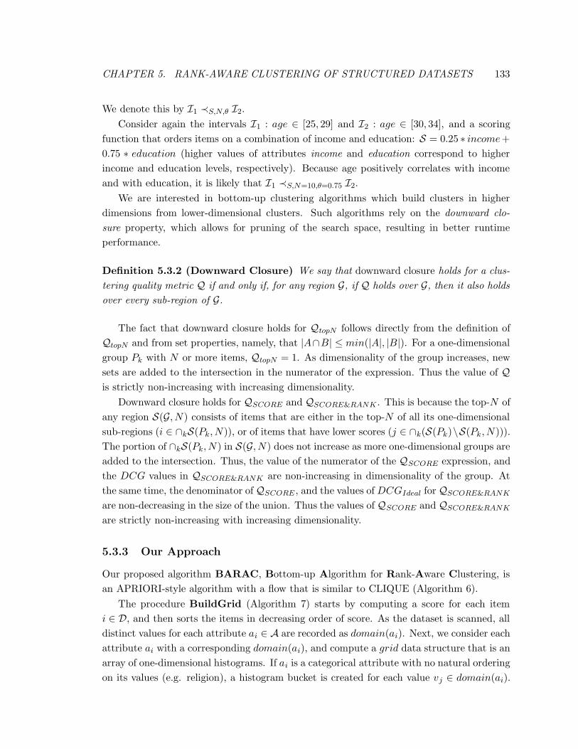
CHAPTER 5. RANK-AWARE CLUSTERING OF STRUCTURED DATASETS 133
We denote this by I1 ≺S,N,θ I2.
Consider again the intervals I1 : age ∈ [25, 29] and I2 : age ∈ [30, 34], and a scoring
function that orders items on a combination of income and education: S = 0.25 ∗ income+
0.75 ∗ education (higher values of attributes income and education correspond to higher
income and education levels, respectively). Because age positively correlates with income
and with education, it is likely that I1 ≺S,N=10,θ=0.75 I2.
We are interested in bottom-up clustering algorithms which build clusters in higher
dimensions from lower-dimensional clusters. Such algorithms rely on the downward clo-
sure property, which allows for pruning of the search space, resulting in better runtime
performance.
Definition 5.3.2 (Downward Closure) We say that downward closure holds for a clus-
tering quality metric Q if and only if, for any region G, if Q holds over G, then it also holds
over every sub-region of G.
The fact that downward closure holds for QtopN follows directly from the definition of
QtopN and from set properties, namely, that |A∩B| ≤ min(|A|, |B|). For a one-dimensional
group Pk with N or more items, QtopN = 1. As dimensionality of the group increases, new
sets are added to the intersection in the numerator of the expression. Thus the value of Q
is strictly non-increasing with increasing dimensionality.
Downward closure holds for QSCORE and QSCORE&RANK . This is because the top-N of
any region S(G, N) consists of items that are either in the top-N of all its one-dimensional
sub-regions (i ∈ ∩kS(Pk, N)), or of items that have lower scores (j ∈ ∩k(S(Pk)\S(Pk, N))).
The portion of ∩kS(Pk, N) in S(G, N) does not increase as more one-dimensional groups are
added to the intersection. Thus, the value of the numerator of the QSCORE expression, and
the DCG values in QSCORE&RANK are non-increasing in dimensionality of the group. At
the same time, the denominator ofQSCORE , and the values of DCGIdeal forQSCORE&RANK
are non-decreasing in the size of the union. Thus the values of QSCORE and QSCORE&RANK
are strictly non-increasing with increasing dimensionality.
5.3.3 Our Approach
Our proposed algorithm BARAC, Bottom-up Algorithm for Rank-Aware Clustering, is
an APRIORI-style algorithm with a flow that is similar to CLIQUE (Algorithm 6).
The procedure BuildGrid (Algorithm 7) starts by computing a score for each item
i ∈ D, and then sorts the items in decreasing order of score. As the dataset is scanned, all
distinct values for each attribute ai ∈ A are recorded as domain(ai). Next, we consider each
attribute ai with a corresponding domain(ai), and compute a grid data structure that is an
array of one-dimensional histograms. If ai is a categorical attribute with no natural ordering
on its values (e.g. religion), a histogram bucket is created for each value vj ∈ domain(ai).
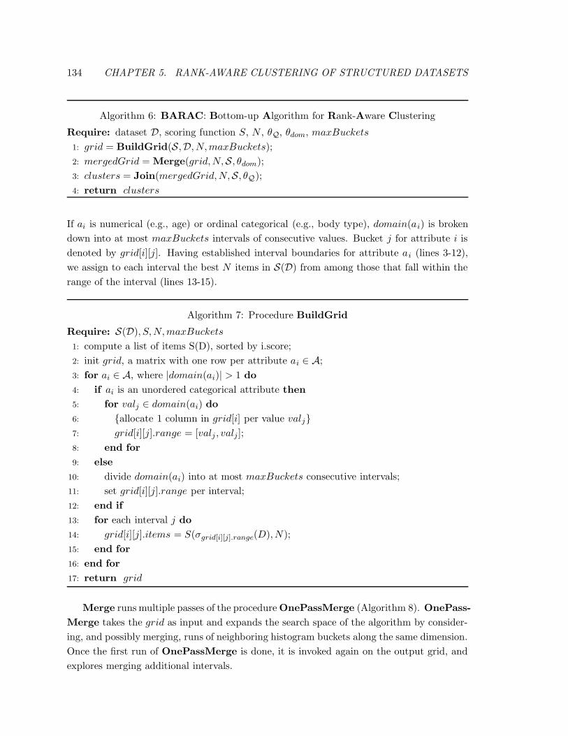
134 CHAPTER 5. RANK-AWARE CLUSTERING OF STRUCTURED DATASETS
Algorithm 6: BARAC: Bottom-up Algorithm for Rank-Aware Clustering
Require: dataset D, scoring function S, N , θQ, θdom, maxBuckets
1: grid = BuildGrid(S,D, N,maxBuckets);
2: mergedGrid = Merge(grid,N,S, θdom);
3: clusters = Join(mergedGrid,N,S, θQ);
4: return clusters
If ai is numerical (e.g., age) or ordinal categorical (e.g., body type), domain(ai) is broken
down into at most maxBuckets intervals of consecutive values. Bucket j for attribute i is
denoted by grid[i][j]. Having established interval boundaries for attribute ai (lines 3-12),
we assign to each interval the best N items in S(D) from among those that fall within the
range of the interval (lines 13-15).
Algorithm 7: Procedure BuildGrid
Require: S(D), S,N,maxBuckets
1: compute a list of items S(D), sorted by i.score;
2: init grid, a matrix with one row per attribute ai ∈ A;
3: for ai ∈ A, where |domain(ai)| > 1 do
4: if ai is an unordered categorical attribute then
5: for valj ∈ domain(ai) do
6: {allocate 1 column in grid[i] per value valj}
7: grid[i][j].range = [valj , valj ];
8: end for
9: else
10: divide domain(ai) into at most maxBuckets consecutive intervals;
11: set grid[i][j].range per interval;
12: end if
13: for each interval j do
14: grid[i][j].items = S(σgrid[i][j].range(D), N);
15: end for
16: end for
17: return grid
Merge runs multiple passes of the procedure OnePassMerge (Algorithm 8). OnePass-
Merge takes the grid as input and expands the search space of the algorithm by consider-
ing, and possibly merging, runs of neighboring histogram buckets along the same dimension.
Once the first run of OnePassMerge is done, it is invoked again on the output grid, and
explores merging additional intervals.
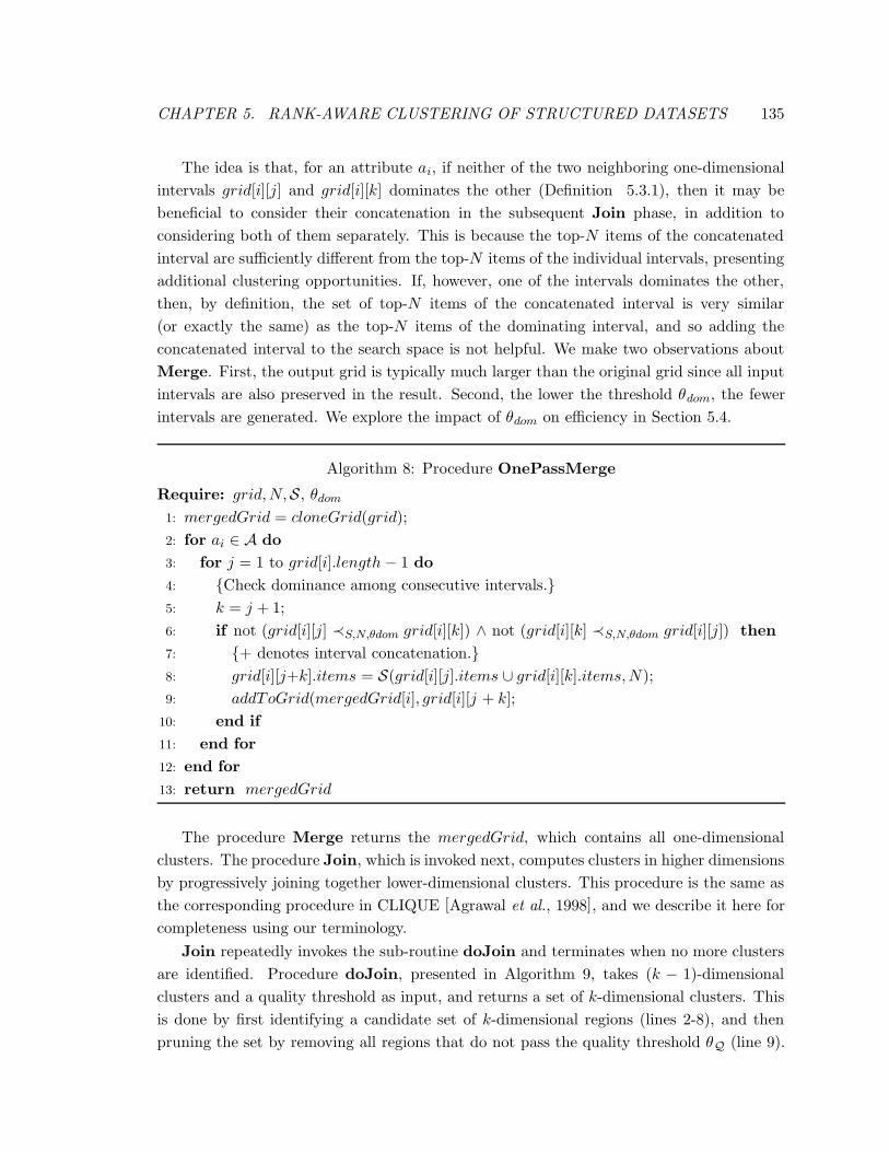
CHAPTER 5. RANK-AWARE CLUSTERING OF STRUCTURED DATASETS 135
The idea is that, for an attribute ai, if neither of the two neighboring one-dimensional
intervals grid[i][j] and grid[i][k] dominates the other (Definition 5.3.1), then it may be
beneficial to consider their concatenation in the subsequent Join phase, in addition to
considering both of them separately. This is because the top-N items of the concatenated
interval are sufficiently different from the top-N items of the individual intervals, presenting
additional clustering opportunities. If, however, one of the intervals dominates the other,
then, by definition, the set of top-N items of the concatenated interval is very similar
(or exactly the same) as the top-N items of the dominating interval, and so adding the
concatenated interval to the search space is not helpful. We make two observations about
Merge. First, the output grid is typically much larger than the original grid since all input
intervals are also preserved in the result. Second, the lower the threshold θdom, the fewer
intervals are generated. We explore the impact of θdom on efficiency in Section 5.4.
Algorithm 8: Procedure OnePassMerge
Require: grid,N,S, θdom
1: mergedGrid = cloneGrid(grid);
2: for ai ∈ A do
3: for j = 1 to grid[i].length − 1 do
4: {Check dominance among consecutive intervals.}
5: k = j + 1;
6: if not (grid[i][j] ≺S,N,θdom grid[i][k]) ∧ not (grid[i][k] ≺S,N,θdom grid[i][j]) then
7: {+ denotes interval concatenation.}
8: grid[i][j+k].items = S(grid[i][j].items ∪ grid[i][k].items,N);
9: addToGrid(mergedGrid[i], grid[i][j + k];
10: end if
11: end for
12: end for
13: return mergedGrid
The procedure Merge returns the mergedGrid, which contains all one-dimensional
clusters. The procedure Join, which is invoked next, computes clusters in higher dimensions
by progressively joining together lower-dimensional clusters. This procedure is the same as
the corresponding procedure in CLIQUE [Agrawal et al., 1998], and we describe it here for
completeness using our terminology.
Join repeatedly invokes the sub-routine doJoin and terminates when no more clusters
are identified. Procedure doJoin, presented in Algorithm 9, takes (k − 1)-dimensional
clusters and a quality threshold as input, and returns a set of k-dimensional clusters. This
is done by first identifying a candidate set of k-dimensional regions (lines 2-8), and then
pruning the set by removing all regions that do not pass the quality threshold θQ (line 9).
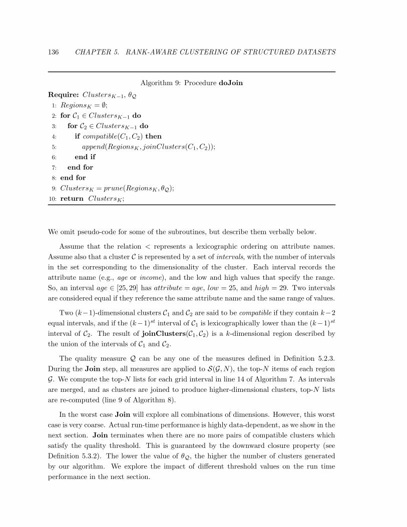
136 CHAPTER 5. RANK-AWARE CLUSTERING OF STRUCTURED DATASETS
Algorithm 9: Procedure doJoin
Require: ClustersK−1, θQ
1: RegionsK = ∅;
2: for C1 ∈ ClustersK−1 do
3: for C2 ∈ ClustersK−1 do
4: if compatible(C1, C2) then
5: append(RegionsK , joinClusters(C1, C2));
6: end if
7: end for
8: end for
9: ClustersK = prune(RegionsK , θQ);
10: return ClustersK;
We omit pseudo-code for some of the subroutines, but describe them verbally below.
Assume that the relation < represents a lexicographic ordering on attribute names.
Assume also that a cluster C is represented by a set of intervals, with the number of intervals
in the set corresponding to the dimensionality of the cluster. Each interval records the
attribute name (e.g., age or income), and the low and high values that specify the range.
So, an interval age ∈ [25, 29] has attribute = age, low = 25, and high = 29. Two intervals
are considered equal if they reference the same attribute name and the same range of values.
Two (k−1)-dimensional clusters C1 and C2 are said to be compatible if they contain k−2
equal intervals, and if the (k−1)st interval of C1 is lexicographically lower than the (k−1)st
interval of C2. The result of joinClusters(C1, C2) is a k-dimensional region described by
the union of the intervals of C1 and C2.
The quality measure Q can be any one of the measures defined in Definition 5.2.3.
During the Join step, all measures are applied to S(G, N), the top-N items of each region
G. We compute the top-N lists for each grid interval in line 14 of Algorithm 7. As intervals
are merged, and as clusters are joined to produce higher-dimensional clusters, top-N lists
are re-computed (line 9 of Algorithm 8).
In the worst case Join will explore all combinations of dimensions. However, this worst
case is very coarse. Actual run-time performance is highly data-dependent, as we show in the
next section. Join terminates when there are no more pairs of compatible clusters which
satisfy the quality threshold. This is guaranteed by the downward closure property (see
Definition 5.3.2). The lower the value of θQ, the higher the number of clusters generated
by our algorithm. We explore the impact of different threshold values on the run time
performance in the next section.
CHAPTER 5. RANK-AWARE CLUSTERING OF STRUCTURED DATASETS 137
5.4 Experimental Evaluation of Performance
We implemented BARAC with our three clustering quality measures (Section 5.2.2.)
Since QSCORE behaved similarly to QtopN , we only report results with the latter and
QSCORE&RANK . Our prototype is implemented in Java and operates on memory-resident
data. All experiments were executed on a 64-bit machine with two Intel Xeon 2.13GHz
processors and 4GB of RAM, running RedHat EL AS 4.
5.4.1 The Yahoo! Personals Dataset
Dataset. We evaluated the performance of BARAC on a dataset from a leading on-
line dating service with millions of registered users. Users of the service create a personal
profile in which they describe themselves using 30 structured attributes, e.g., age, height,
occupation, education, income, etc. Users also commonly store one or several target profiles,
expressed in terms of the same structured attributes. When specifying that profile, users
designate attributes as required and desirable. Required attributes are used as filtering
conditions for exact matching against personal profiles, while desirable attributes are used
for ranking exact matches.
For the purpose of our experiments we focus on computing matches for male users,
as there are at least one order of magnitude more males searching for females. We store
a snapshot of target profiles of male users whom we call seekers, and of personal profiles
of female users. The snapshot is as of a recent month in 2008, and contains all profiles
that were registered with the dating service up to and including that month. We use
19 of the total 30 attributes, because there was no meaningful correlation between the
ignored attributes (e.g. astrological sign) and other attributes, making them less suitable
for clustering. Two of the 19 attributes, has photo and gender, have only two distinct values,
and we use them for filtering, but not for clustering. So, there are 19 filtering attributes
and 17 clustering attributes in our dataset. Therefore, for any given query, the number of
clustering dimensions is at most 17.
User Sampling. We evaluated the performance for 100 target profiles. We chose
a representative sample of profiles that cover a range of filtering and ranking attributes,
as well as different number of matches. The chosen target profiles specify between 3 and
15 filtering attributes (median 5), and between 1 and 6 ranking attributes (median 3).
Because data exploration is most meaningful for large datasets, we selected profiles with at
least 1,000 matches for our evaluation. Our prototype operates on memory-resident data,
and does all processing in memory. Due to a limitation in available RAM, we restrict our
attention to users whose target profiles match up to 500,000 profiles. The chosen target
profiles generated between 1,107 and 489,090 matches (median 102,492). Note that the size
of the result set will often be reduced in practice by applying additional filtering criteria
such as geographic distance between the seeker and the match, the freshness of the profile
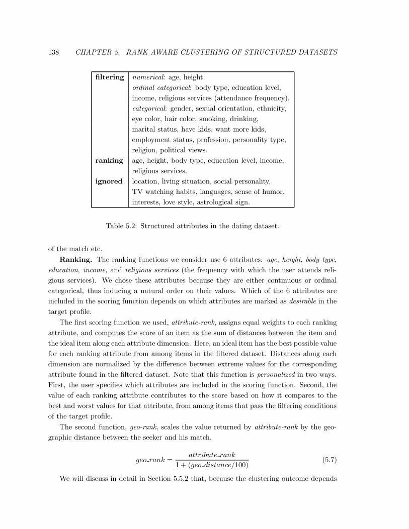
138 CHAPTER 5. RANK-AWARE CLUSTERING OF STRUCTURED DATASETS
filtering numerical: age, height.
ordinal categorical: body type, education level,
income, religious services (attendance frequency).
categorical: gender, sexual orientation, ethnicity,
eye color, hair color, smoking, drinking,
marital status, have kids, want more kids,
employment status, profession, personality type,
religion, political views.
ranking age, height, body type, education level, income,
religious services.
ignored location, living situation, social personality,
TV watching habits, languages, sense of humor,
interests, love style, astrological sign.
Table 5.2: Structured attributes in the dating dataset.
of the match etc.
Ranking. The ranking functions we consider use 6 attributes: age, height, body type,
education, income, and religious services (the frequency with which the user attends reli-
gious services). We chose these attributes because they are either continuous or ordinal
categorical, thus inducing a natural order on their values. Which of the 6 attributes are
included in the scoring function depends on which attributes are marked as desirable in the
target profile.
The first scoring function we used, attribute-rank, assigns equal weights to each ranking
attribute, and computes the score of an item as the sum of distances between the item and
the ideal item along each attribute dimension. Here, an ideal item has the best possible value
for each ranking attribute from among items in the filtered dataset. Distances along each
dimension are normalized by the difference between extreme values for the corresponding
attribute found in the filtered dataset. Note that this function is personalized in two ways.
First, the user specifies which attributes are included in the scoring function. Second, the
value of each ranking attribute contributes to the score based on how it compares to the
best and worst values for that attribute, from among items that pass the filtering conditions
of the target profile.
The second function, geo-rank, scales the value returned by attribute-rank by the geo-
graphic distance between the seeker and his match.
geo rank =attribute rank
1 + (geo distance/100)(5.7)
We will discuss in detail in Section 5.5.2 that, because the clustering outcome depends
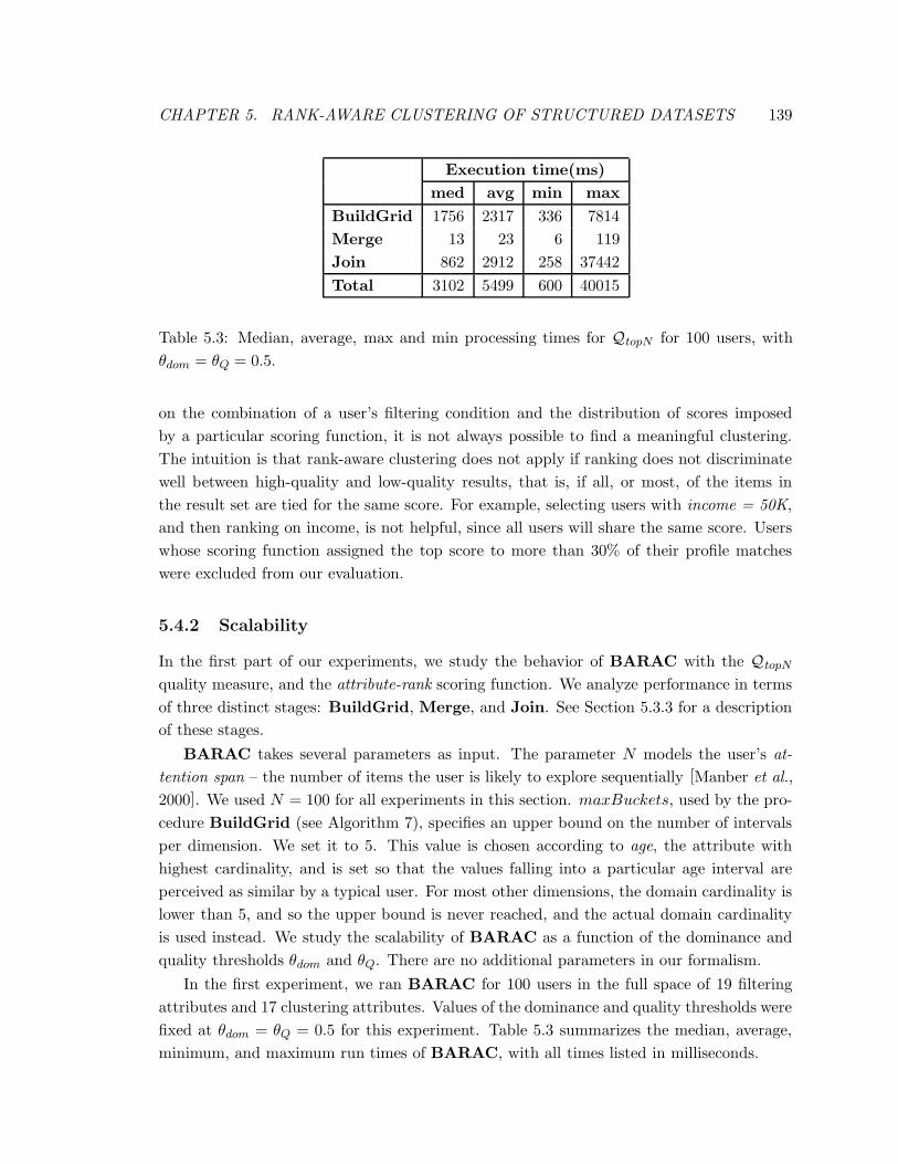
CHAPTER 5. RANK-AWARE CLUSTERING OF STRUCTURED DATASETS 139
Execution time(ms)
med avg min max
BuildGrid 1756 2317 336 7814
Merge 13 23 6 119
Join 862 2912 258 37442
Total 3102 5499 600 40015
Table 5.3: Median, average, max and min processing times for QtopN for 100 users, with
θdom = θQ = 0.5.
on the combination of a user’s filtering condition and the distribution of scores imposed
by a particular scoring function, it is not always possible to find a meaningful clustering.
The intuition is that rank-aware clustering does not apply if ranking does not discriminate
well between high-quality and low-quality results, that is, if all, or most, of the items in
the result set are tied for the same score. For example, selecting users with income = 50K,
and then ranking on income, is not helpful, since all users will share the same score. Users
whose scoring function assigned the top score to more than 30% of their profile matches
were excluded from our evaluation.
5.4.2 Scalability
In the first part of our experiments, we study the behavior of BARAC with the QtopN
quality measure, and the attribute-rank scoring function. We analyze performance in terms
of three distinct stages: BuildGrid, Merge, and Join. See Section 5.3.3 for a description
of these stages.
BARAC takes several parameters as input. The parameter N models the user’s at-
tention span – the number of items the user is likely to explore sequentially [Manber et al.,
2000]. We used N = 100 for all experiments in this section. maxBuckets, used by the pro-
cedure BuildGrid (see Algorithm 7), specifies an upper bound on the number of intervals
per dimension. We set it to 5. This value is chosen according to age, the attribute with
highest cardinality, and is set so that the values falling into a particular age interval are
perceived as similar by a typical user. For most other dimensions, the domain cardinality is
lower than 5, and so the upper bound is never reached, and the actual domain cardinality
is used instead. We study the scalability of BARAC as a function of the dominance and
quality thresholds θdom and θQ. There are no additional parameters in our formalism.
In the first experiment, we ran BARAC for 100 users in the full space of 19 filtering
attributes and 17 clustering attributes. Values of the dominance and quality thresholds were
fixed at θdom = θQ = 0.5 for this experiment. Table 5.3 summarizes the median, average,
minimum, and maximum run times of BARAC, with all times listed in milliseconds.
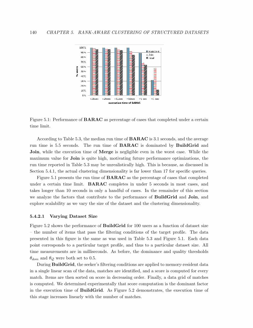
140 CHAPTER 5. RANK-AWARE CLUSTERING OF STRUCTURED DATASETS
Figure 5.1: Performance of BARAC as percentage of cases that completed under a certain
time limit.
According to Table 5.3, the median run time of BARAC is 3.1 seconds, and the average
run time is 5.5 seconds. The run time of BARAC is dominated by BuildGrid and
Join, while the execution time of Merge is negligible even in the worst case. While the
maximum value for Join is quite high, motivating future performance optimizations, the
run time reported in Table 5.3 may be unrealistically high. This is because, as discussed in
Section 5.4.1, the actual clustering dimensionality is far lower than 17 for specific queries.
Figure 5.1 presents the run time of BARAC as the percentage of cases that completed
under a certain time limit. BARAC completes in under 5 seconds in most cases, and
takes longer than 10 seconds in only a handful of cases. In the remainder of this section
we analyze the factors that contribute to the performance of BuildGrid and Join, and
explore scalability as we vary the size of the dataset and the clustering dimensionality.
5.4.2.1 Varying Dataset Size
Figure 5.2 shows the performance of BuildGrid for 100 users as a function of dataset size
– the number of items that pass the filtering conditions of the target profile. The data
presented in this figure is the same as was used in Table 5.3 and Figure 5.1. Each data
point corresponds to a particular target profile, and thus to a particular dataset size. All
time measurements are in milliseconds. As before, the dominance and quality thresholds
θdom and θQ were both set to 0.5.
During BuildGrid, the seeker’s filtering conditions are applied to memory-resident data
in a single linear scan of the data, matches are identified, and a score is computed for every
match. Items are then sorted on score in decreasing order. Finally, a data grid of matches
is computed. We determined experimentally that score computation is the dominant factor
in the execution time of BuildGrid. As Figure 5.2 demonstrates, the execution time of
this stage increases linearly with the number of matches.
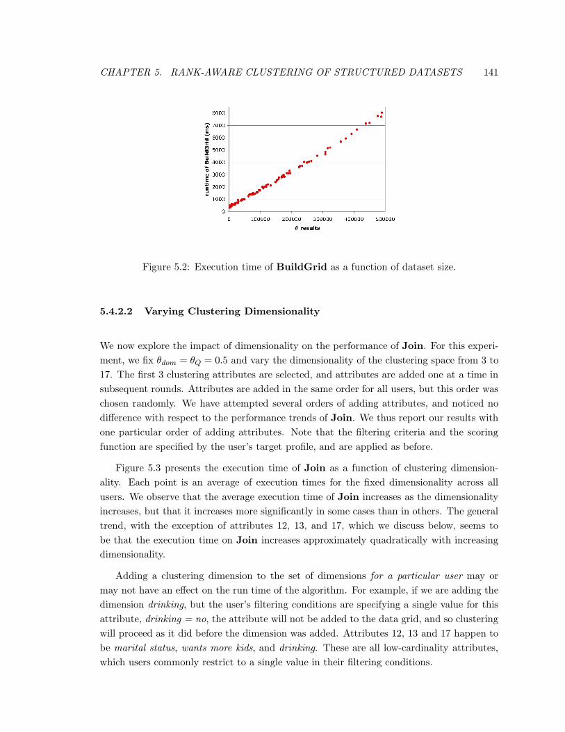
CHAPTER 5. RANK-AWARE CLUSTERING OF STRUCTURED DATASETS 141
Figure 5.2: Execution time of BuildGrid as a function of dataset size.
5.4.2.2 Varying Clustering Dimensionality
We now explore the impact of dimensionality on the performance of Join. For this experi-
ment, we fix θdom = θQ = 0.5 and vary the dimensionality of the clustering space from 3 to
17. The first 3 clustering attributes are selected, and attributes are added one at a time in
subsequent rounds. Attributes are added in the same order for all users, but this order was
chosen randomly. We have attempted several orders of adding attributes, and noticed no
difference with respect to the performance trends of Join. We thus report our results with
one particular order of adding attributes. Note that the filtering criteria and the scoring
function are specified by the user’s target profile, and are applied as before.
Figure 5.3 presents the execution time of Join as a function of clustering dimension-
ality. Each point is an average of execution times for the fixed dimensionality across all
users. We observe that the average execution time of Join increases as the dimensionality
increases, but that it increases more significantly in some cases than in others. The general
trend, with the exception of attributes 12, 13, and 17, which we discuss below, seems to
be that the execution time on Join increases approximately quadratically with increasing
dimensionality.
Adding a clustering dimension to the set of dimensions for a particular user may or
may not have an effect on the run time of the algorithm. For example, if we are adding the
dimension drinking, but the user’s filtering conditions are specifying a single value for this
attribute, drinking = no, the attribute will not be added to the data grid, and so clustering
will proceed as it did before the dimension was added. Attributes 12, 13 and 17 happen to
be marital status, wants more kids, and drinking. These are all low-cardinality attributes,
which users commonly restrict to a single value in their filtering conditions.
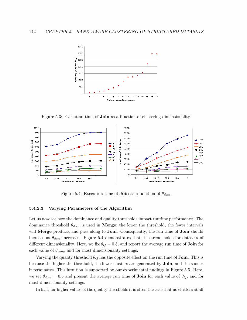
142 CHAPTER 5. RANK-AWARE CLUSTERING OF STRUCTURED DATASETS
Figure 5.3: Execution time of Join as a function of clustering dimensionality.
Figure 5.4: Execution time of Join as a function of θdom.
5.4.2.3 Varying Parameters of the Algorithm
Let us now see how the dominance and quality thresholds impact runtime performance. The
dominance threshold θdom is used in Merge; the lower the threshold, the fewer intervals
will Merge produce, and pass along to Join. Consequently, the run time of Join should
increase as θdom increases. Figure 5.4 demonstrates that this trend holds for datasets of
different dimensionality. Here, we fix θQ = 0.5, and report the average run time of Join for
each value of θdom, and for most dimensionality settings.
Varying the quality threshold θQ has the opposite effect on the run time of Join. This is
because the higher the threshold, the fewer clusters are generated by Join, and the sooner
it terminates. This intuition is supported by our experimental findings in Figure 5.5. Here,
we set θdom = 0.5 and present the average run time of Join for each value of θQ, and for
most dimensionality settings.
In fact, for higher values of the quality thresholds it is often the case that no clusters at all
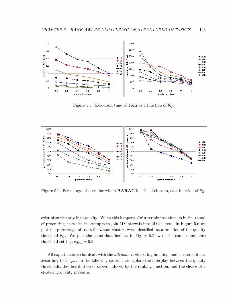
CHAPTER 5. RANK-AWARE CLUSTERING OF STRUCTURED DATASETS 143
Figure 5.5: Execution time of Join as a function of θQ.
Figure 5.6: Percentage of users for whom BARAC identified clusters, as a function of θQ.
exist of sufficiently high quality. When this happens, Join terminates after its initial round
of processing, in which it attempts to join 1D intervals into 2D clusters. In Figure 5.6 we
plot the percentage of users for whom clusters were identified, as a function of the quality
threshold θQ. We plot the same data here as in Figure 5.5, with the same dominance
threshold setting, θdom = 0.5.
All experiments so far dealt with the attribute-rank scoring function, and clustered items
according to QtopN . In the following section, we explore the interplay between the quality
thresholds, the distribution of scores induced by the ranking function, and the choice of a
clustering quality measure.
144 CHAPTER 5. RANK-AWARE CLUSTERING OF STRUCTURED DATASETS
5.5 Effectiveness of Rank-Aware Clustering: A Qualitative
Analysis
5.5.1 Clustering Quality
We now give a qualitative intuition of the kinds of clusters that are discovered by BARAC.
We use the QtopN quality metric, and the attribute-rank ranking function for the purpose of
this evaluation. We focus our attention on the following set of filtering conditions that are
in-line with our motivating example in Section 5.1: age ∈ [25,35], height ∈ [160cm, 175cm],
education ≥ Bachelor’s, ethnicity = Caucasian, body type ∈ {slim, slender, average, athletic,
fit}.
This set of filtering conditions returns over 30,000 matches. We rank the matches on
a combination of income and education, both from higher to lower. There are about 100
top-matches: women with post-graduate education who make more than $150K. About two
thirds of the top matches are over 29 years old, and so younger matches would not be easily
accessible if results were returned as a ranked list.
Let us now cluster the results of BARAC, using the QtopN quality metric. The following
are some of the clusters that are returned and that deal directly with the correlation between
income and age, and income and education:
• age ∈ [25, 27] ∧ income ∈ [$35K, $75K]
• age ∈ [28, 33] ∧ income ∈ [$75K, $150K]
• age ∈ [28, 33] ∧ income ≥ $150K
• age ∈ [31, 35] ∧ income ≥ $75K
• age ∈ [28, 33] ∧ education = post graduate
• age ∈ [31, 35] ∧ education = post graduate
Note that two clusters are returned that contain different sets of matches with age
between 28 and 33. Note also that the younger matches, aged between 25 and 27, are
returned as a cluster with relatively lower income. These matches would not have been
easily accessible in a single ranked list. BARAC also returned several clusters that are
not directly related to the ranking conditions, but for which a correlation was detected
among attributes at top ranks. So, there was a cluster of matches who are politically very
conservative or conservative and who attend religious services more than once a week or
weekly. Another cluster consisted of matches who are politically middle of the road or
liberal and who attend religious services no more often than monthly.
Recall that BARAC does not partition the dataset. That is, an item may be returned as
part of one or several clusters. This is a feature of our approach that bears some similarity to
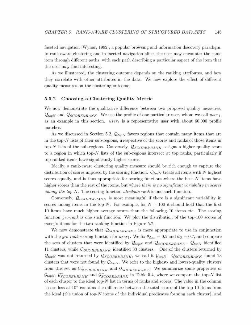
CHAPTER 5. RANK-AWARE CLUSTERING OF STRUCTURED DATASETS 145
faceted navigation [Wynar, 1992], a popular browsing and information discovery paradigm.
In rank-aware clustering and in faceted navigation alike, the user may encounter the same
item through different paths, with each path describing a particular aspect of the item that
the user may find interesting.
As we illustrated, the clustering outcome depends on the ranking attributes, and how
they correlate with other attributes in the data. We now explore the effect of different
quality measures on the clustering outcome.
5.5.2 Choosing a Clustering Quality Metric
We now demonstrate the qualitative difference between two proposed quality measures,
QtopN and QSCORE&RANK . We use the profile of one particular user, whom we call user1,
as an example in this section. user1 is a representative user with about 60,000 profile
matches.
As we discussed in Section 5.2, QtopN favors regions that contain many items that are
in the top-N lists of their sub-regions, irrespective of the scores and ranks of those items in
top-N lists of the sub-regions. Conversely, QSCORE&RANK assigns a higher quality score
to a region in which top-N lists of the sub-regions intersect at top ranks, particularly if
top-ranked items have significantly higher scores.
Ideally, a rank-aware clustering quality measure should be rich enough to capture the
distribution of scores imposed by the scoring function. QtopN treats all items with N highest
scores equally, and is thus appropriate for scoring functions where the best N items have
higher scores than the rest of the items, but where there is no significant variability in scores
among the top-N . The scoring function attribute-rank is one such function.
Conversely, QSCORE&RANK is most meaningful if there is a significant variability in
scores among items in the top-N . For example, for N = 100 it should hold that the first
10 items have much higher average scores than the following 10 items etc. The scoring
function geo-rank is one such function. We plot the distribution of the top-100 scores of
user1’s items for the two ranking function in Figure 5.7.
We now demonstrate that QSCORE&RANK is more appropriate to use in conjunction
with the geo-rank scoring function for user1. We fix θdom = 0.5 and θQ = 0.7, and compare
the sets of clusters that were identified by QtopN and QSCORE&RANK . QtopN identified
11 clusters, while QSCORE&RANK identified 33 clusters. One of the clusters returned by
QtopN was not returned by QSCORE&RANK , we call it GtopN . QSCORE&RANK found 23
clusters that were not found by QtopN . We refer to the highest- and lowest-quality clusters
from this set as G+SCORE&RANK and G−SCORE&RANK . We summarize some properties of
GtopN , G+SCORE&RANK and G−SCORE&RANK in Table 5.4, where we compare the top-N list
of each cluster to the ideal top-N list in terms of ranks and scores. The value in the column
“score loss at 10” contains the difference between the total scores of the top-10 items from
the ideal (the union of top-N items of the individual predicates forming each cluster), and
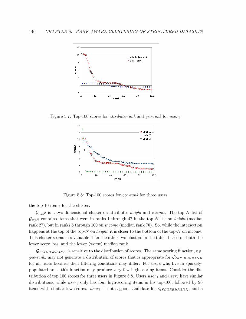
146 CHAPTER 5. RANK-AWARE CLUSTERING OF STRUCTURED DATASETS
Figure 5.7: Top-100 scores for attribute-rank and geo-rank for user1.
Figure 5.8: Top-100 scores for geo-rank for three users.
the top-10 items for the cluster.
GtopN is a two-dimensional cluster on attributes height and income. The top-N list of
GtopN contains items that were in ranks 1 through 47 in the top-N list on height (median
rank 27), but in ranks 8 through 100 on income (median rank 70). So, while the intersection
happens at the top of the top-N on height, it is closer to the bottom of the top-N on income.
This cluster seems less valuable than the other two clusters in the table, based on both the
lower score loss, and the lower (worse) median rank.
QSCORE&RANK is sensitive to the distribution of scores. The same scoring function, e.g.
geo-rank, may not generate a distribution of scores that is appropriate for QSCORE&RANK
for all users because their filtering conditions may differ. For users who live in sparsely-
populated areas this function may produce very few high-scoring items. Consider the dis-
tribution of top 100 scores for three users in Figure 5.8. Users user1 and user2 have similar
distributions, while user3 only has four high-scoring items in his top-100, followed by 96
items with similar low scores. user3 is not a good candidate for QSCORE&RANK , and a
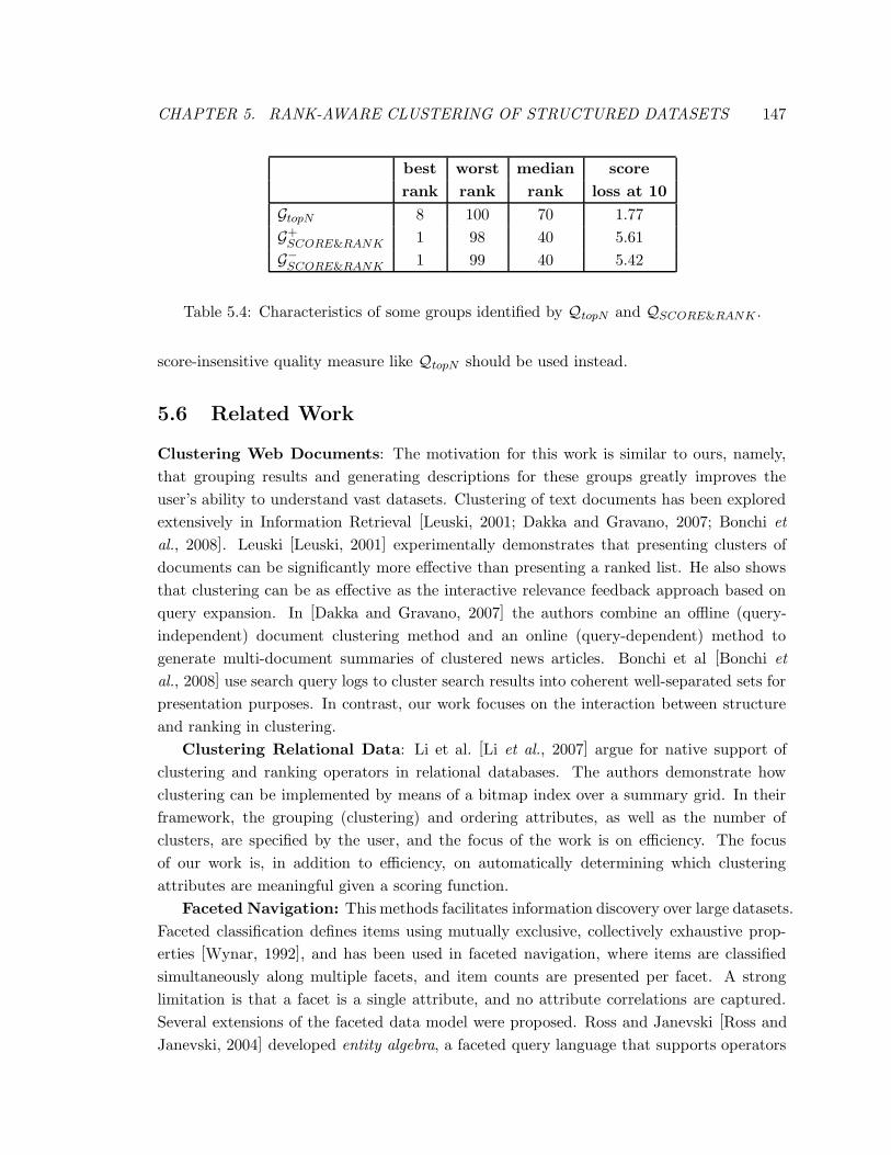
CHAPTER 5. RANK-AWARE CLUSTERING OF STRUCTURED DATASETS 147
best worst median score
rank rank rank loss at 10
GtopN 8 100 70 1.77
G+SCORE&RANK 1 98 40 5.61
G−SCORE&RANK 1 99 40 5.42
Table 5.4: Characteristics of some groups identified by QtopN and QSCORE&RANK .
score-insensitive quality measure like QtopN should be used instead.
5.6 Related Work
Clustering Web Documents: The motivation for this work is similar to ours, namely,
that grouping results and generating descriptions for these groups greatly improves the
user’s ability to understand vast datasets. Clustering of text documents has been explored
extensively in Information Retrieval [Leuski, 2001; Dakka and Gravano, 2007; Bonchi et
al., 2008]. Leuski [Leuski, 2001] experimentally demonstrates that presenting clusters of
documents can be significantly more effective than presenting a ranked list. He also shows
that clustering can be as effective as the interactive relevance feedback approach based on
query expansion. In [Dakka and Gravano, 2007] the authors combine an offline (query-
independent) document clustering method and an online (query-dependent) method to
generate multi-document summaries of clustered news articles. Bonchi et al [Bonchi et
al., 2008] use search query logs to cluster search results into coherent well-separated sets for
presentation purposes. In contrast, our work focuses on the interaction between structure
and ranking in clustering.
Clustering Relational Data: Li et al. [Li et al., 2007] argue for native support of
clustering and ranking operators in relational databases. The authors demonstrate how
clustering can be implemented by means of a bitmap index over a summary grid. In their
framework, the grouping (clustering) and ordering attributes, as well as the number of
clusters, are specified by the user, and the focus of the work is on efficiency. The focus
of our work is, in addition to efficiency, on automatically determining which clustering
attributes are meaningful given a scoring function.
Faceted Navigation: This methods facilitates information discovery over large datasets.
Faceted classification defines items using mutually exclusive, collectively exhaustive prop-
erties [Wynar, 1992], and has been used in faceted navigation, where items are classified
simultaneously along multiple facets, and item counts are presented per facet. A strong
limitation is that a facet is a single attribute, and no attribute correlations are captured.
Several extensions of the faceted data model were proposed. Ross and Janevski [Ross and
Janevski, 2004] developed entity algebra, a faceted query language that supports operators
148 CHAPTER 5. RANK-AWARE CLUSTERING OF STRUCTURED DATASETS
such as selection and semi-join. Ben-Yitzhak et al. [Ben-Yitzhak et al., 2008] extended
faceted navigation to include quantitative summary information other than item counts,
such as average price and rating, and developed methods for efficient computation of such
statistics over correlated facets.
Roy et al. [Roy et al., 2008] proposed techniques that dynamically suggest facets for
database exploration, with the goal of minimizing navigation time. At every step, the
system asks the user a set of questions about his information need, and dynamically fetches
the next most promising set of facets. In [Dash et al., 2008], the authors extend Solr, a
popular search engine, with dynamic faceted search for exploring data with both textual
content and structured attributes. Given a keyword query, the system selects a small set of
interesting attributes, where interestingness measures the difference between expected and
actual attribute values.
Our work is complementary to faceted navigation. While we focus on attribute correla-
tions, our analysis can be used to propose to the user which, among many attributes, may
be more interesting to explore in a particular dataset.
The Many-Answers Problem: In [Chaudhuri et al., 2004] the authors state the
Many-Answers Problem and show how correlations among attribute values in a structured
datasets can be used to automatically derive a suitable ranking function. To this end,
the authors develop a comprehensive probabilistic information retrieval ranking model and
present efficient processing techniques. A related Empty-Answers Problem is discussed
in [Agrawal et al., 2003]. Here, the authors present an adaptation of inverse document
frequency (IDF) that is used for automatic ranking of results. The authors also propose to
incorporate workload information into the ranking.
Rank Aggregation: Fagin et al. [Fagin et al., 2003b] propose rank aggregation, in
which ranked exploration of large high dimensional datasets is viewed as a similarity search
problem. Given a ranking function on d attributes, the algorithm considers d ranked lists,
and aggregates these lists using a variant of the threshold algorithm [Fagin et al., 2003c].
An approximation based on dimensionality reduction is also proposed, in which projections
along random lines in the d-dimensional space are taken, and the computation is carried
out on the projection.
Our work differs from [Fagin et al., 2003b] in that we consider non-ranking attributes
in addition to the ranking attributes. Rather than computing a global aggregate rank or
similarity score, we consider the correlations that hold among attributes of the data in
various projections of the space, and identify items, or groups of items, that are best from
among comparable, given the ranking function.
Skyline Operator: A alternative result presentation method in presence of multi-
dimensional ranking functions is the skyline [Borzsonyi et al., 2001]. A point in multi-
dimensional space is said to belong to the skyline if it is not dominated by any other point,
i.e., if no other point is as good or better in all dimensions, and strictly better in at least
CHAPTER 5. RANK-AWARE CLUSTERING OF STRUCTURED DATASETS 149
one dimension. In Chapter 3 we presented a skyline visualization of ranked results in a
two-dimensional space. Skylines are a valuable data visualization tool, however, the results
of this visualization are difficult to interpret for datasets of high dimensionality. The notion
of dominance may be applicable to other aspects of our work, such as cluster selection, and
we plan to consider this direction in the future.
Integrating Ranking with Clustering: Sun et al. [Sun et al., 2009] recently pre-
sented RankClus, a framework that integrates ranking with clustering in a heterogeneous
information network such as DBLP. RankClus is based on a mixture model that uses mutual
reinforcement between clustering and ranking. Our high-level motivation is also to treat
clustering and ranking as parts of a unified framework. However, our application domain
(structured datasets with user-defined ranking functions) and technical approach are very
different.
5.7 Conclusion
In this chapter we introduced rank-aware clustering, a novel result presentation method
for large structured datasets. We developed rank-aware clustering quality measures, and
proposed BARAC: a Bottom-up Algorithm for Rank-Aware Clustering, an Apriori-style
algorithm geared specifically at such quality measures. We presented an extensive exper-
imental evaluation of scalability, and gave an intuition of the effectiveness of BARAC on
Yahoo! Personals datasets. A large-scale user study is currently underway in scope of the
Yahoo! Research Sandbox project. The goal of the study is to ascertain the effect of our
result presentation method on the user experience. We look forward to reporting these
results in a subsequent study. In the future we will consider performance optimizations,
and will explore the applicability of our methods to other large structured datasets. We
will also explore user interface design issues such as cluster selection.

150 CHAPTER 5. RANK-AWARE CLUSTERING OF STRUCTURED DATASETS
CHAPTER 6. OTHER CONTRIBUTIONS 151
Chapter 6
Other Contributions
This chapter summarizes some work that is not directly related to the main theme of this
thesis, but that was carried out as part of the doctoral research.
6.1 Data Modeling in Complex Domains
6.1.1 Schema Polynomials and Applications
This section is based on joint work with Kenneth A. Ross and appeared in [Ross and
Stoyanovich, 2008].
Conceptual complexity is emerging as a new bottleneck as database developers, appli-
cation developers, and database administrators struggle to design and comprehend large,
complex schemas. Applications in domains as diverse as medicine, archaeology, and astron-
omy often rest on database schemas with hundreds of relations and thousands of columns.
The schema design and maintenance, as well as application development, are all extremely
challenging for schemas of this size.
The conciseness of a schema depends critically on the idioms available to express the
schema. As an analogy, consider the class of boolean expressions with conjunction and
disjunction. It is well known that there are formulas that are compact in one representation
(say disjunctive normal form) but exponentially bigger in another (say conjunctive normal
form), and vice versa.
Three well-known formalisms for writing schemas are the relational, the object-oriented,
and the faceted approaches. Each of these is very good at expressing certain classes of
schema, but poor at expressing certain other classes of schema. Object-oriented schemas
allow the factorization of common attributes into an inheritance hierarchy. Faceted schemas
allow the orthogonal composition of many independent attributes; in an e-commerce appli-
cation, for example, a product may be independently classified by size, by brand, and by
color. Traditionally, one has been limited to just one of these design methodologies when
152 CHAPTER 6. OTHER CONTRIBUTIONS
creating schemas. However, even if part of the schema is compactly represented using that
methodology, other parts may not be.
We define a higher-level conceptual data representation language that allows the schema
to be manipulated in ways that expose the strengths of each of these data modeling ap-
proaches. If a schema has parts that are compact when expressed according to one approach,
then that part of the schema should be expressed using that approach, even if other parts
of the schema use a different approach. We propose a formal language for representing
schemas, and derive a set of properties that allow one to manipulate schema expressions
while preserving the set of representable tuples. We propose that standard design method-
ologies such as entity-relationship modeling [Ramakrishnan and Gehrke, 2003], modeling
in UML [Booch et al., 2005], faceted modeling [Wynar, 1992], and relational normaliza-
tion [Ramakrishnan and Gehrke, 2003], produce outputs in this framework rather than
going directly to a physical relational schema, with the following advantages:
• One can explore a variety of physical representations obtained using different equiva-
lent expressions for a schema.
• One can derive an unambiguous logical representation that allows transformations,
such as attribute factorization and subtraction, that are not straightforward for sets
of physical tables.
• Different users can orient the schema to their own points of view. One user may
impose an inheritance hierarchy (e.g., factoring out the location of manufacture) while
another may impose an alternative hierarchy (e.g., factoring out the product-type).
These conceptual views are compatible, and can be automatically translated into the
chosen physical representation.
• Users can project out parts of the schema that they are not interested in. The remain-
ing portion can be simplified using various equivalences, leading to a description that
is much easier to understand than a schema with hundreds of tables and thousands
of columns.
Our novel schema modeling framework, which we call schema polynomials, reasons over
schema expressions. The basic notion in describing schemas is the attribute: a label, along
with a data type, that represents an aspect of a concept. Examples of attributes are “age”,
“height”, “company-name”, etc. We use attributes to define tuple-descriptors:
Definition 6.1.1 A tuple-descriptor T is defined recursively with the context free grammar:
T ::= 0 | 1 | A | B | C | . . . | TT | T + T | T − T
We will describe the concatenation TT as multiplication. A, B, C, . . . are the attribute
names, 1 is a special symbol denoting an empty product (i.e., the empty set of attributes),
and 0 is a special symbol denoting an empty sum. �
CHAPTER 6. OTHER CONTRIBUTIONS 153
In [Ross and Stoyanovich, 2008] we demonstrate how tuple-descriptors may be used to
concisely represent schemas, and we illustrate this here with an example. Consider the
following schema expression.
ABCD + ABG + ACD + AG + BCH (6.1)
When we write ABCD in Expression 6.1 we mean that tuples with attribute names A,
B, C, and D are valid for this schema. When we write S1 +S2 we mean that a tuple is valid
for either S1 or S2. Our schema could be mapped to a collection of five stored tables ABCD,
ABG, ACD, AG, and BCH. We use bold script to describe physical level structures such
as tables, and math script for conceptual level expressions. We could alternatively factorize
the schema into the representation:
A(B + 1)(CD + G) + BCH (6.2)
This representation has fewer syntactic elements than Expression 6.1. Common occur-
rences of some attributes have been factored out. The B + 1 subexpression allows tuples
having either a valid or a null value for attribute B. Expression 6.2 does not have a direct
relational interpretation, since there is no relational construct to express CD + G. Never-
theless, one can map this expression to a set of tables for storage as follows: Add a new
unique identifier column (say I) to represent the link between the A(B + 1) subexpression
and the (CD + G) subexpression, to yield tables ABI, ICD, IG and BCH, where B can
be null in ABI. This transformation is correct only with constraints on the new attribute
I. The constraint for I in ABI says that the value of I must appear in exactly one of ICD
and IG. There must also be foreign key constraints on I into ABI from both ICD and IG.
An alternative rewriting of Expression 6.2 is:
A(B + 1)[(CD + 1)(G + 1)− CDG− 1] + BCH (6.3)
The subtractions in Expression 6.3 can be interpreted as constraints stating that (a) C,
D, and G cannot all be non-null, and (b) C, D, and G cannot all be null. This expression can
be mapped to a physical schema ABCDG, BCH, where ABCDG has various null/not-
null constraints on B, C, D, and G. If one cared only about attributes A, B, and C in
this schema, one could project out the other attributes to obtain from Expresssion 6.1 the
simpler expression ABC + AB + AC + A + BC, which could again be factorized in various
ways. Yet another factorization of Expression 6.1 is:
C(ABD + AD + BH) + ABG + AG (6.4)
This would be a natural factorization in a hierarchical or object-oriented view in which C
is the primary dimension of classification and is inherited from a higher-level entity. Unlike
traditional object-oriented data modeling that imposes a single hierarchical structure, our
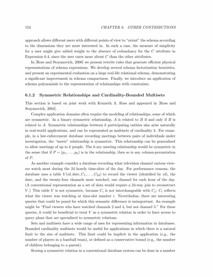
154 CHAPTER 6. OTHER CONTRIBUTIONS
approach allows different users with different points of view to “orient” the schema according
to the dimensions they are most interested in. In such a case, the measure of simplicity
for a user might give added weight to the absence of redundancy for the C attribute in
Expression 6.4, since the user cares more about C than the other attributes.
In [Ross and Stoyanovich, 2008] we present rewrite rules that generate efficient physical
representations of schema expressions. We develop several schema factorization heuristics,
and present an experimental evaluation on a large real-life relational schema, demonstrating
a significant improvement in schema compactness. Finally, we introduce an application of
schema polynomials to the representation of relationships with constraints.
6.1.2 Symmetric Relationships and Cardinality-Bounded Multisets
This section is based on joint work with Kenneth A. Ross and appeared in [Ross and
Stoyanovich, 2004].
Complex application domains often require the modeling of relationships, some of which
are symmetric. In a binary symmetric relationship, A is related to B if and only if B is
related to A. Symmetric relationships between k participating entities also arise naturally
in real-world applications, and can be represented as multisets of cardinality k. For exam-
ple, in a law-enforcement database recording meetings between pairs of individuals under
investigation, the “meets” relationship is symmetric. This relationship can be generalized
to allow meetings of up to k people. The k-ary meeting relationship would be symmetric in
the sense that if P = (p1, . . . , pk) is in the relationship, then so is any column-permutation
of P .
As another example consider a database recording what television channel various view-
ers watch most during the 24 hourly time-slots of the day. For performance reasons, the
database uses a table V (id, date, C1, . . . , C24) to record the viewer (identified by id), the
date, and the twenty-four channels most watched, one channel for each hour of the day.
(A conventional representation as a set of slots would require a 24-way join to reconstruct
V .) This table V is not symmetric, because Ci is not interchangeable with Cj: Ci reflects
what the viewer was watching at time-slot number i. Nevertheless, there are interesting
queries that could be posed for which this semantic difference is unimportant. An example
might be “Find viewers who have watched channels 2 and 4, but not channel 5.” For these
queries, it could be beneficial to treat V as a symmetric relation in order to have access to
query plans that are specialized to symmetric relations.
Sets and multisets have a wide range of uses for representing information in databases.
Bounded cardinality multisets would be useful for applications in which there is a natural
limit to the size of multisets. This limit could be implicit in the application (e.g., the
number of players in a baseball team), or defined as a conservative bound (e.g., the number
of children belonging to a parent).
Storing a symmetric relation in a conventional database system can be done in a number
CHAPTER 6. OTHER CONTRIBUTIONS 155
of possible ways. Storing the full symmetric relation induces some redundancy in the
database: more space is required (up to a factor of k! for k-ary relationships), and integrity
constraints need to be enforced to ensure consistency of updates. Updates need to be aware
of the symmetry of the table, and to add the various column permutations to all insertions
and deletions. Queries need to perform I/O for tuples and their permutations, increasing
the time needed for query processing.
Alternatively, a database schema designer could recognize that the relation was sym-
metric and code database procedures to store only one representative tuple for each group
of permuted tuples. A view can then be defined to present the symmetric closure of the
stored relation for query processing. The update problem remains, because updates through
this view would be ambiguous. Updates to the underlying table would need to be aware of
the symmetry, to avoid storing multiple permutations of a tuple, and to perform a deletion
correctly. For symmetric relations over k columns, just defining the view using standard
SQL requires a query of length proportional to k(k!).
For both of the above proposals, indexed access to an underlying symmetric relationship
would require multiple index lookups, one for each symmetric column.
A third alternative is to model a symmetric relation as a set [Date, 2003] or multiset.
Instead of recording both R(a, b, c, d, e) and R(b, a, c, d, e), one could record R ′(q, c, d, e),
S(a, q), and S(b, q), where q is a new surrogate identifier, and R ′ and S are new tables. The
intuition here is that q represents a multiset, of which a and b are members according to table
S. Distinct members of the multiset can be substituted for the first two arguments of R. To
represent tuples that are their own symmetric complement, such as R(a, a, c, d, e), one inserts
S(a, q) twice. This representation uses slightly more space than the previous proposal, while
not resolving the issue of keeping the representation consistent under updates. Further,
reconstructing the original symmetric relation requires joins.
In [Ross and Stoyanovich, 2004] we argue that none of these solutions is ideal, and that
the database system should be responsible for providing a symmetric table type. We propose
techniques to enable such a table type, and provide:
• An underlying abstract data type to store the kernel of a symmetric relation, i.e.,
a particular non-redundant subset of the relation. We show how updates on this
data type would be handled by the database system. We describe how relational
normalization techniques should take account of symmetric relations during database
design. Both normalization and the proposed representation of symmetric relations
aim to remove redundancy, so combining these two approaches should be beneficial.
• An extension of the relational algebra with a symmetric closure operator γ. We show
how to translate a query over a symmetric relation into a query involving γ applied to
the kernel of the relation. We provide algebraic equivalences that allow the rewriting
of queries so that work can be saved by applying γ as late as possible.
156 CHAPTER 6. OTHER CONTRIBUTIONS
• A method for inferring when a view is guaranteed to be symmetric. By using this
method, the database system has the flexibility to store a materialized view using the
more compact representation.
• A syntactic extension to SQL that allows the succinct expression of queries over sym-
metric relations.
6.1.3 A Faceted Query Engine Applied to Archaeology
This section is based on joint work with Kenneth A. Ross and Angel Janevski, and appeared
in [Ross et al., 2005; Ross et al., 2007].
A number of application domains require the modeling of complex entities within classi-
fication hierarchies. For many of these domains, the hierarchy and the entity structure are
the main sources of complexity, while other features of the domain, such as relationships
between entities, are relatively simple. In such domains it is natural to make the set of
entities the basic conceptual structure.
Faceted classification was introduced by an Indian librarian and classificationist S.R.
Ranganathan, and was first used in his Colon Classification in the early 1930s. Faceted clas-
sification treats entities or groups of entities as collections of clearly defined, mutually exclu-
sive, and collectively exhaustive aspects, properties or characteristics, called facets [Wynar,
1992]. For example, in an archaeology domain, we may classify artifacts along multiple
orthogonal dimensions: by time period, by culture, by material, or by geographic location.
Recent work, see for example flamenco.berkeley.edu and facetmap.com, proposes
search facilities for hierarchical data using faceted hierarchies. Ross and Janevski [Ross
and Janevski, 2004] developed a faceted data model, and proposed a query language, called
Entity Algebra, that is appropriate for faceted domains. The primary goal of their work was
to create a data model and a query language that is understandable to non-technical users,
while still allowing one to compose complex queries from simple pieces.
Building on the work of [Ross and Janevski, 2004] we developed the Faceted Query En-
gine. Our work was part of an inter-disciplinary project that aims to apply computational
tools from Robotics, Virtual Environments, and Databases to modeling, visualizing, and
analyzing historical and archaeological sites (see www.learn.columbia.edu/nsf). We col-
laborated with archaeologists to create a collection of orthogonal hierarchical classifications
of finds from two archaeological excavations: a large-scale dig of ancient artifacts in Mem-
phis, Egypt [Giddy, 1999], and a medium-scale dig of iron-age finds from Thulamela, South
Africa. Our system provides a web-based user interface, and allows one to query thousands
of objects from the two locations with respect to any of the facets, and to perform spa-
tial and temporal analysis of the data. Users of our system can access text, images, and
multimedia data related to the finds.
Figure 6.1 provides a screenshot of our system with data from the Thulamela excavation.
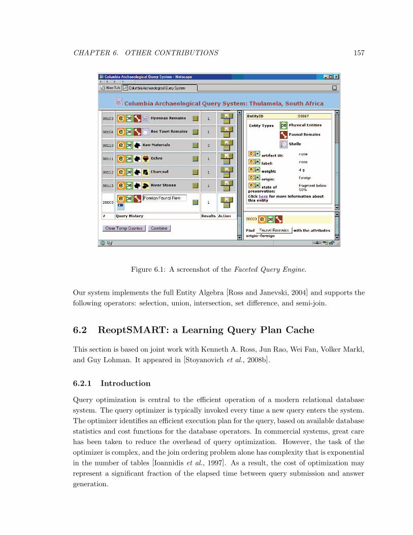
CHAPTER 6. OTHER CONTRIBUTIONS 157
Figure 6.1: A screenshot of the Faceted Query Engine.
Our system implements the full Entity Algebra [Ross and Janevski, 2004] and supports the
following operators: selection, union, intersection, set difference, and semi-join.
6.2 ReoptSMART: a Learning Query Plan Cache
This section is based on joint work with Kenneth A. Ross, Jun Rao, Wei Fan, Volker Markl,
and Guy Lohman. It appeared in [Stoyanovich et al., 2008b].
6.2.1 Introduction
Query optimization is central to the efficient operation of a modern relational database
system. The query optimizer is typically invoked every time a new query enters the system.
The optimizer identifies an efficient execution plan for the query, based on available database
statistics and cost functions for the database operators. In commercial systems, great care
has been taken to reduce the overhead of query optimization. However, the task of the
optimizer is complex, and the join ordering problem alone has complexity that is exponential
in the number of tables [Ioannidis et al., 1997]. As a result, the cost of optimization may
represent a significant fraction of the elapsed time between query submission and answer
generation.
158 CHAPTER 6. OTHER CONTRIBUTIONS
If identical queries are submitted, the database system can cache the optimizer’s plan the
first time, and avoid re-optimization for subsequent query invocations. The query processor
merely has to check for syntactic identity of the query with the cached query. This idea can
be generalized to queries with parameters. Constants in the query are replaced with “bind
variables” to generate a query template, in which the bind variables are parameters. The
query processor can then cache a plan for a query template rather than for a query. As
a result, frequently-submitted queries that differ only in the constants can avoid the cost
of query optimization. Oracle provides such a facility, as do IBM DB2 and Microsoft SQL
Server.
There is a potential problem with this approach. A single plan is chosen for all instances
of a query template. This plan, while optimal in a particular region of the parameter space,
may be sub-optimal in another region. Savings achieved by not invoking the query optimizer
may be nullified by the choice of a sub-optimal execution plan. In fact often the difference
in cost between the optimizer’s plan and the cached plan exceeds the optimization time.
Modern transaction processing systems are often required to handle thousands of trans-
actions per second. Consider for example a web-based OLTP application, such as an on-line
book store described by the TPCW benchmark (www.tpc.org/tpcw). The system executes
canned queries that share a small number of pre-defined templates, such as queries gen-
erated by the same HTML form, but differ in parameter values. An interactive system is
expected to complete query processing and return results to the user in a short amount of
time, often less than a second. A single user’s queries may exhibit locality in the values of
the submitted parameters, in which case a single query execution plan may be good enough.
However, this locality is lost when many users interact with the system at any given time.
Therefore, to ensure that an optimal plan is chosen for every query invocation, every in-
stance of the query must be optimized anew. Many of these queries involve joins of several
database tables and are thus non-trivial to optimize. In this setting, query optimization
may add significant overhead to the overall execution time.
Parametric query optimization (PQO) models the distribution of plans chosen in differ-
ent regions of the parameter space of a query template [Hulgeri and Sudarshan, 2003], or of
a set of templates [Ghosh et al., 2002]. A PQO system is trained off-line using a number of
invocations of the query optimizer on instances of the query template. The result of such
training is a function that, given an instance of the query parameters, identifies a plan that
is likely to be the optimizer’s choice. To be useful, this function must execute quickly, much
faster than the optimizer itself. The function must also have a compact representation, so
that a collection of such functions can be managed in memory by the database system.
In [Stoyanovich et al., 2008b] we present ReoptSMART, a parametric query optimization
framework that uses machine learning techniques to analyze the training set, and to generate
a set of classifiers that map parameter instances to plans.
Compared with earlier geometric approaches [Hulgeri and Sudarshan, 2003], machine
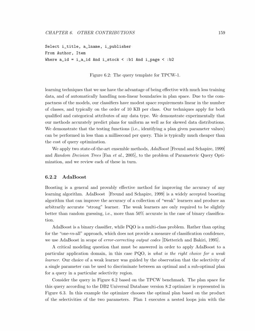
CHAPTER 6. OTHER CONTRIBUTIONS 159
Select i_title, a_lname, i_publisher
From Author, Item
Where a_id = i_a_id And i_stock < :b1 And i_page < :b2
Figure 6.2: The query template for TPCW-1.
learning techniques that we use have the advantage of being effective with much less training
data, and of automatically handling non-linear boundaries in plan space. Due to the com-
pactness of the models, our classifiers have modest space requirements linear in the number
of classes, and typically on the order of 10 KB per class. Our techniques apply for both
qualified and categorical attributes of any data type. We demonstrate experimentally that
our methods accurately predict plans for uniform as well as for skewed data distributions.
We demonstrate that the testing functions (i.e., identifying a plan given parameter values)
can be performed in less than a millisecond per query. This is typically much cheaper than
the cost of query optimization.
We apply two state-of-the-art ensemble methods, AdaBoost [Freund and Schapire, 1999]
and Random Decision Trees [Fan et al., 2005], to the problem of Parameteric Query Opti-
mization, and we review each of these in turn.
6.2.2 AdaBoost
Boosting is a general and provably effective method for improving the accuracy of any
learning algorithm. AdaBoost [Freund and Schapire, 1999] is a widely accepted boosting
algorithm that can improve the accuracy of a collection of “weak” learners and produce an
arbitrarily accurate “strong” learner. The weak learners are only required to be slightly
better than random guessing, i.e., more than 50% accurate in the case of binary classifica-
tion.
AdaBoost is a binary classifier, while PQO is a multi-class problem. Rather than opting
for the “one-vs-all” approach, which does not provide a measure of classification confidence,
we use AdaBoost in scope of error-correcting output codes [Dietterich and Bakiri, 1995].
A critical modeling question that must be answered in order to apply AdaBoost to a
particular application domain, in this case PQO, is what is the right choice for a weak
learner. Our choice of a weak learner was guided by the observation that the selectivity of
a single parameter can be used to discriminate between an optimal and a sub-optimal plan
for a query in a particular selectivity region.
Consider the query in Figure 6.2 based on the TPCW benchmark. The plan space for
this query according to the DB2 Universal Database version 8.2 optimizer is represented in
Figure 6.3. In this example the optimizer chooses the optimal plan based on the product
of the selectivities of the two parameters. Plan 1 executes a nested loops join with the
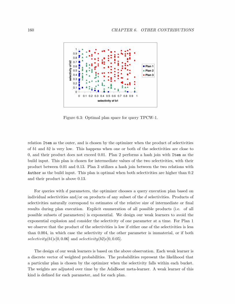
160 CHAPTER 6. OTHER CONTRIBUTIONS
00.10.20.30.40.50.60.70.80.9
1
0 0.1 0.2 0.3 0.4 0.5 0.6 0.7 0.8 0.9 1selectivity of b1
sele
ctiv
ity o
f b2
Plan 1Plan 2Plan 3
Figure 6.3: Optimal plan space for query TPCW-1.
relation Item as the outer, and is chosen by the optimizer when the product of selectivities
of b1 and b2 is very low. This happens when one or both of the selectivities are close to
0, and their product does not exceed 0.01. Plan 2 performs a hash join with Item as the
build input. This plan is chosen for intermediate values of the two selectivities, with their
product between 0.01 and 0.13. Plan 3 utilizes a hash join between the two relations with
Author as the build input. This plan is optimal when both selectivities are higher than 0.2
and their product is above 0.13.
For queries with d parameters, the optimizer chooses a query execution plan based on
individual selectivities and/or on products of any subset of the d selectivities. Products of
selectivities naturally correspond to estimates of the relative size of intermediate or final
results during plan execution. Explicit enumeration of all possible products (i.e. of all
possible subsets of parameters) is exponential. We design our weak learners to avoid the
exponential explosion and consider the selectivity of one parameter at a time. For Plan 1
we observe that the product of the selectivities is low if either one of the selectivities is less
than 0.004, in which case the selectivity of the other parameter is immaterial, or if both
selectivity(b1)ε[0, 0.06] and selectivity(b2)ε[0, 0.05].
The design of our weak learners is based on the above observation. Each weak learner is
a discrete vector of weighted probabilities. The probabilities represent the likelihood that
a particular plan is chosen by the optimizer when the selectivity falls within each bucket.
The weights are adjusted over time by the AdaBoost meta-learner. A weak learner of this
kind is defined for each parameter, and for each plan.
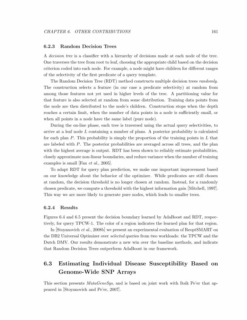
CHAPTER 6. OTHER CONTRIBUTIONS 161
6.2.3 Random Decision Trees
A decision tree is a classifier with a hierarchy of decisions made at each node of the tree.
One traverses the tree from root to leaf, choosing the appropriate child based on the decision
criterion coded into each node. For example, a node might have children for different ranges
of the selectivity of the first predicate of a query template.
The Random Decision Tree (RDT) method constructs multiple decision trees randomly.
The construction selects a feature (in our case a predicate selectivity) at random from
among those features not yet used in higher levels of the tree. A partitioning value for
that feature is also selected at random from some distribution. Training data points from
the node are then distributed to the node’s children. Construction stops when the depth
reaches a certain limit, when the number of data points in a node is sufficiently small, or
when all points in a node have the same label (pure node).
During the on-line phase, each tree is traversed using the actual query selectivities, to
arrive at a leaf node L containing a number of plans. A posterior probability is calculated
for each plan P . This probability is simply the proportion of the training points in L that
are labeled with P . The posterior probabilities are averaged across all trees, and the plan
with the highest average is output. RDT has been shown to reliably estimate probabilities,
closely approximate non-linear boundaries, and reduce variance when the number of training
examples is small [Fan et al., 2005].
To adapt RDT for query plan prediction, we make one important improvement based
on our knowledge about the behavior of the optimizer. While predicates are still chosen
at random, the decision threshold is no longer chosen at random. Instead, for a randomly
chosen predicate, we compute a threshold with the highest information gain [Mitchell, 1997].
This way we are more likely to generate pure nodes, which leads to smaller trees.
6.2.4 Results
Figures 6.4 and 6.5 present the decision boundary learned by AdaBoost and RDT, respec-
tively, for query TPCW-1. The color of a region indicates the learned plan for that region.
In [Stoyanovich et al., 2008b] we present an experimental evaluation of ReoptSMART on
the DB2 Universal Optimizer over selected queries from two workloads: the TPCW and the
Dutch DMV. Our results demonstrate a new win over the baseline methods, and indicate
that Random Decision Trees outperform AdaBoost in our framework.
6.3 Estimating Individual Disease Susceptibility Based on
Genome-Wide SNP Arrays
This section presents MutaGeneSys, and is based on joint work with Itsik Pe’er that ap-
peared in [Stoyanovich and Pe’er, 2007].
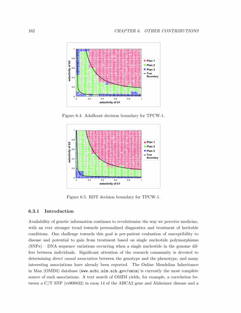
162 CHAPTER 6. OTHER CONTRIBUTIONS
0
0.2
0.4
0.6
0.8
1
0 0.2 0.4 0.6 0.8 1
Plan 1
Plan 2
Plan 3
True
Boundary
selectivity of b1
sele
cti
vit
y o
f b
2
Figure 6.4: AdaBoost decision boundary for TPCW-1.
0
0.2
0.4
0.6
0.8
1
0 0.2 0.4 0.6 0.8 1
Plan 1
Plan 2
Plan 3
True
Boundary
selectivity of b1
sele
cti
vit
y o
f b
2
Figure 6.5: RDT decision boundary for TPCW-1.
6.3.1 Introduction
Availability of genetic information continues to revolutionize the way we perceive medicine,
with an ever stronger trend towards personalized diagnostics and treatment of heritable
conditions. One challenge towards this goal is per-patient evaluation of susceptibility to
disease and potential to gain from treatment based on single nucleotide polymorphisms
(SNPs) – DNA sequence variations occurring when a single nucleotide in the genome dif-
fers between individuals. Significant attention of the research community is devoted to
determining direct causal association between the genotype and the phenotype, and many
interesting associations have already been reported. The Online Mendelian Inheritance
in Man (OMIM) database (www.ncbi.nlm.nih.gov/omim) is currently the most complete
source of such associations. A text search of OMIM yields, for example, a correlation be-
tween a C/T SNP (rs908832) in exon 14 of the ABCA2 gene and Alzheimer disease and a
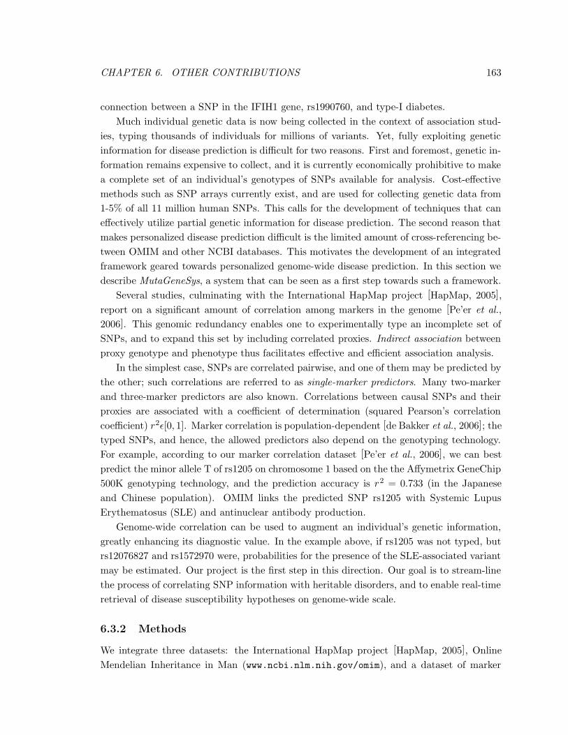
CHAPTER 6. OTHER CONTRIBUTIONS 163
connection between a SNP in the IFIH1 gene, rs1990760, and type-I diabetes.
Much individual genetic data is now being collected in the context of association stud-
ies, typing thousands of individuals for millions of variants. Yet, fully exploiting genetic
information for disease prediction is difficult for two reasons. First and foremost, genetic in-
formation remains expensive to collect, and it is currently economically prohibitive to make
a complete set of an individual’s genotypes of SNPs available for analysis. Cost-effective
methods such as SNP arrays currently exist, and are used for collecting genetic data from
1-5% of all 11 million human SNPs. This calls for the development of techniques that can
effectively utilize partial genetic information for disease prediction. The second reason that
makes personalized disease prediction difficult is the limited amount of cross-referencing be-
tween OMIM and other NCBI databases. This motivates the development of an integrated
framework geared towards personalized genome-wide disease prediction. In this section we
describe MutaGeneSys, a system that can be seen as a first step towards such a framework.
Several studies, culminating with the International HapMap project [HapMap, 2005],
report on a significant amount of correlation among markers in the genome [Pe’er et al.,
2006]. This genomic redundancy enables one to experimentally type an incomplete set of
SNPs, and to expand this set by including correlated proxies. Indirect association between
proxy genotype and phenotype thus facilitates effective and efficient association analysis.
In the simplest case, SNPs are correlated pairwise, and one of them may be predicted by
the other; such correlations are referred to as single-marker predictors. Many two-marker
and three-marker predictors are also known. Correlations between causal SNPs and their
proxies are associated with a coefficient of determination (squared Pearson’s correlation
coefficient) r2ε[0, 1]. Marker correlation is population-dependent [de Bakker et al., 2006]; the
typed SNPs, and hence, the allowed predictors also depend on the genotyping technology.
For example, according to our marker correlation dataset [Pe’er et al., 2006], we can best
predict the minor allele T of rs1205 on chromosome 1 based on the the Affymetrix GeneChip
500K genotyping technology, and the prediction accuracy is r2 = 0.733 (in the Japanese
and Chinese population). OMIM links the predicted SNP rs1205 with Systemic Lupus
Erythematosus (SLE) and antinuclear antibody production.
Genome-wide correlation can be used to augment an individual’s genetic information,
greatly enhancing its diagnostic value. In the example above, if rs1205 was not typed, but
rs12076827 and rs1572970 were, probabilities for the presence of the SLE-associated variant
may be estimated. Our project is the first step in this direction. Our goal is to stream-line
the process of correlating SNP information with heritable disorders, and to enable real-time
retrieval of disease susceptibility hypotheses on genome-wide scale.
6.3.2 Methods
We integrate three datasets: the International HapMap project [HapMap, 2005], Online
Mendelian Inheritance in Man (www.ncbi.nlm.nih.gov/omim), and a dataset of marker
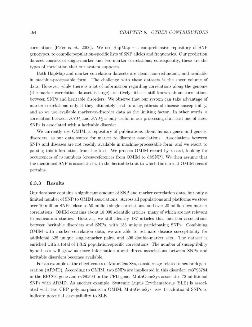
164 CHAPTER 6. OTHER CONTRIBUTIONS
correlations [Pe’er et al., 2006]. We use HapMap – a comprehensive repository of SNP
genotypes, to compile population-specific lists of SNP alleles and frequencies. Our prediction
dataset consists of single-marker and two-marker correlations; consequently, these are the
types of correlation that our system supports.
Both HapMap and marker correlation datasets are clean, non-redundant, and available
in machine-processable form. The challenge with these datasets is the sheer volume of
data. However, while there is a lot of information regarding correlations along the genome
(the marker correlation dataset is large), relatively little is still known about correlations
between SNPs and heritable disorders. We observe that our system can take advantage of
marker correlations only if they ultimately lead to a hypothesis of disease susceptibility,
and so we use available marker-to-disorder data as the limiting factor. In other words, a
correlation between SNP1 and SNP2 is only useful in our processing if at least one of these
SNPs is associated with a heritable disorder.
We currently use OMIM, a repository of publications about human genes and genetic
disorders, as our data source for marker to disorder associations. Associations between
SNPs and diseases are not readily available in machine-processable form, and we resort to
parsing this information from the text. We process OMIM record by record, looking for
occurrences of rs numbers (cross-references from OMIM to dbSNP). We then assume that
the mentioned SNP is associated with the heritable trait to which the current OMIM record
pertains.
6.3.3 Results
Our database contains a significant amount of SNP and marker correlation data, but only a
limited number of SNP to OMIM associations. Across all populations and platforms we store
over 10 million SNPs, close to 50 million single correlations, and over 20 million two-marker
correlations. OMIM contains about 18,000 scientific articles, many of which are not relevant
to association studies. However, we still identify 187 articles that mention associations
between heritable disorders and SNPs, with 133 unique participating SNPs. Combining
OMIM with marker correlation data, we are able to estimate disease susceptibility for
additional 328 unique single-marker pairs, and 396 double-marker sets. The dataset is
enriched with a total of 1,312 population-specific correlations. The number of susceptibility
hypotheses will grow as more information about direct associations between SNPs and
heritable disorders becomes available.
For an example of the effectiveness of MutaGeneSys, consider age-related macular degen-
eration (ARMD). According to OMIM, two SNPs are implicated in this disorder: rs3793784
in the ERCC6 gene and rs380390 in the CFH gene. MutaGeneSys associates 72 additional
SNPs with ARMD. As another example, Systemic Lupus Erythematosus (SLE) is associ-
ated with two CRP polymorphisms in OMIM; MutaGeneSys uses 15 additional SNPs to
indicate potential susceptibility to SLE.
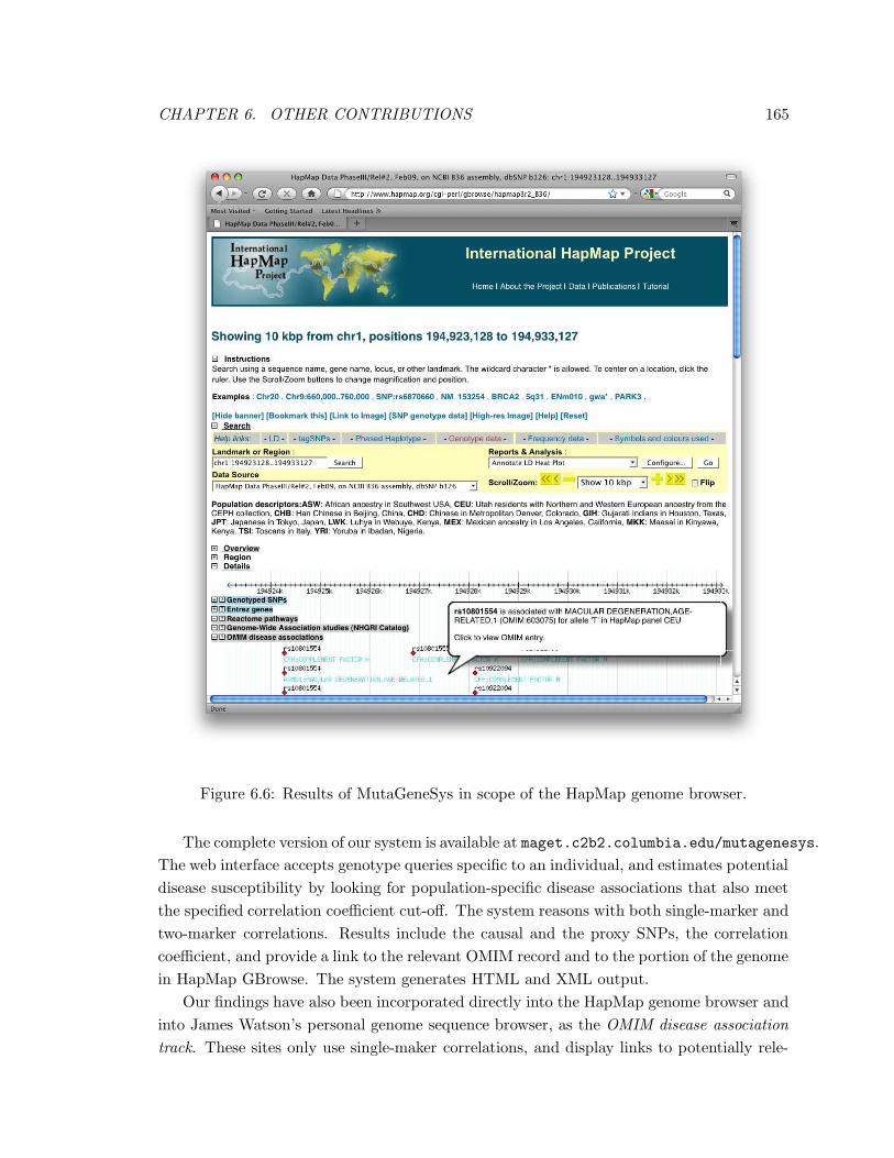
CHAPTER 6. OTHER CONTRIBUTIONS 165
Figure 6.6: Results of MutaGeneSys in scope of the HapMap genome browser.
The complete version of our system is available at maget.c2b2.columbia.edu/mutagenesys.
The web interface accepts genotype queries specific to an individual, and estimates potential
disease susceptibility by looking for population-specific disease associations that also meet
the specified correlation coefficient cut-off. The system reasons with both single-marker and
two-marker correlations. Results include the causal and the proxy SNPs, the correlation
coefficient, and provide a link to the relevant OMIM record and to the portion of the genome
in HapMap GBrowse. The system generates HTML and XML output.
Our findings have also been incorporated directly into the HapMap genome browser and
into James Watson’s personal genome sequence browser, as the OMIM disease association
track. These sites only use single-maker correlations, and display links to potentially rele-
166 CHAPTER 6. OTHER CONTRIBUTIONS
vant OMIM records irrespective of the population and of the coefficient of determination.
Figure 6.6 presents a view of our findings for a particular region on Chromosome 1, as part
of the HapMap genome browser.
6.3.4 Discussion
MutaGeneSys cannot yet be considered a source of diagnostic predictions, because of a num-
ber of uncertainties involved in going from a specific marker to disease. Given the available
data, we made our best effort to control for population and correlation-specific effects:
marker associations are computed separately for different populations, and susceptibility
results include correlation parameters. For lack of information, we make two assumptions
about OMIM markers: that they are causal, and that they correspond to the minor allele.
(We incorporate allele frequencies from HapMap to determine which allele to consider as
minor in a particular population.) Another source of uncertainty is that specific markers
may have different levels of penetrance, and therefore have different value as diagnostic
predictors. Because of these factors we are currently only able to estimate, not diagnose,
individual disease susceptibility.
CHAPTER 7. CONCLUSION 167
Chapter 7
Conclusion
In this thesis we proposed novel search and ranking techniques that improve the user expe-
rience and facilitate information discovery in several semantically rich application domains.
We showed how the social context in social tagging sites can be used for user-centric in-
formation discovery. We proposed novel ontology-aware search and ranking techniques,
and applied them to scientific literature search and to ranking in Wikipedia. We addressed
data exploration in ranked structured datasets, and proposed a rank-aware clustering algo-
rithm that uses semantic relationships among attributes of high-quality items to facilitate
information discovery.
7.1 Summary of Contributions
We now elaborate on our technical contributions and outline some promising future direc-
tions.
In Chapter 2 we described the goals and challenges of context-aware ranking on the
Social Web. We showed how a user’s social behavior in a collaborative tagging site can
be used to improve the quality of content recommendation. We presented network-aware
search, a novel search paradigm where the score of an item is computed based on a user’s
social network. We showed how the standard top-K processing algorithms can be used for
network-aware search, and presented performance optimizations that explore the trade-off
between query processing time and space overhead. We provided an extensive experimental
evaluation of our techniques on a dataset from Delicious, a leading social tagging site.
Our techniques improve the current state of the art in search and ranking on the So-
cial Web, but also reach beyond social tagging sites, and towards incorporating the social
dimension into general Web search.
In Chapter 3 we tackled the challenge of enhancing relevance ranking in scientific lit-
erature search. We describe PubMed, the largest bibliographic source in the domain of
life sciences, and consider how a large high-quality ontology of Medical Subject Headings
168 CHAPTER 7. CONCLUSION
(MeSH) can be used to relate a user’s query to the annotations of a document. We ob-
served that the MeSH hierarchy is scoped, i.e., terms may appear in multiple places in the
hierarchy, and the meaning of a term depends on its position. This observation challenges
most past work which has been developed assuming that a term has a unique node in the
generalization hierarchy.
We developed several relevance measures appropriate for ranking in the domain at hand,
and proposed efficient evaluation algorithms for computing relevance on the scale of PubMed
and MeSH. We have demonstrated that our measures can be computed in interactive time
using score upper-bounds. We presented a two-dimensional Skyline visualization of query
results that facilitates data exploration, and demonstrated that it, too, can be computed
efficiently on the scale of PubMed and MeSH.
We also presented results of a preliminary user study that evaluates the effectiveness
of our techniques. The small scale of our study and the complexity of evaluation do not
allow us to draw statistically significant conclusions about the relative performance of our
methods and baselines. In the future we plan to make our software available to the scientific
community. This will increase the practical impact of our research and will allow us to gather
more information about the effectiveness of our methods.
In Chapter 4 we developed an entity-aware ranking framework, and presented a novel
ranking algorithm, EntityAuthority, that models the mutual reinforcement between pages
and entities. We demonstrated how an ontology can be used for query processing in this set-
ting. We presented a prototype implementation of our system, and experimentally demon-
strated the improvement in query result quality.
In Chapter 5 we introduced rank-aware clustering, a novel result presentation method
for large structured datasets. We developed rank-aware clustering quality measures, and
proposed a Bottom-up Algorithm for Rank-Aware Clustering (BARAC), an Apriori-style
algorithm geared specifically at such quality measures. We presented an extensive exper-
imental evaluation of scalability, and gave an intuition of the effectiveness of BARAC on
Yahoo! Personals datasets.
A large-scale user study is currently underway in scope of the Yahoo! Research Sandbox
project. The goal of the study is to ascertain the effect of our result presentation method
on the user experience. In the future we will consider performance optimizations, and will
explore the applicability of our methods to other large structured datasets. We will also
explore user interface design issues such as cluster selection.
7.2 Future Research Directions
7.2.1 Combining Different Types of Semantic Context
Using semantic context for search and ranking has potential for high impact, both in terms
of scientific advances in Data Management and by enabling end-users. An important ques-
CHAPTER 7. CONCLUSION 169
tion that I will address in the future is how to combine various types of context into a
single model, achieving higher expressive power, and ultimately supporting a better user
experience.
The techniques described in this thesis can be extended and applied to the domain of life
sciences, with the goal of facilitating customized content recommendation and scientific col-
laboration. In a hypothetical system called PubMed Social, a scientist’s profile may include
ontology terms that describe his research interests. The scientist may establish a network
of collaborators, and may choose to customize his search and information discovery experi-
ence by incorporating his semantic (ontology-based) or social (network-based) context. In
addition to consuming available content, the scientist may use the system to disseminate
his findings. He will do so by annotating results, and by sharing them with other members
of his network. Depending on the stage of the project, the scientist may choose to share
results with a small group of collaborators, or with the scientific community at large.
In certain situations, the quality of ranking in search and in content recommendation
may be improved by incorporating the user’s mental context, or intent, into the model.
This is based on the observation that the information need may be different for the same
user in different situations: I may ask my mother’s advise on cooking, and my academic
adviser’s opinion on research. Likewise, a user of PubMed Social who participates in inter-
disciplinary research, or who is active in multiple research areas, may need help from the
system when choosing and aggregating information from multiple sources. To this end, I
will explore how structured contextual information about the user, about a particular task,
and about the nature of the user’s relationship with the content, can be used to better
organize information feeds.
The paradigm of an information feed, or channel, has emerged as the de-facto stan-
dard for information aggregation and sharing in syndicated and collaborative environments.
Some examples include the use of RSS for blog aggregation, Facebook’s news feed function-
ality, and status updates on Twitter. Feeds are typically used to aggregate and serve recent
information, and are well-suited for accessing information in order of publication time, from
more to less recent. However, important information that was published outside the most
recent visible time window may be missed. Further, while organizing information solely
by time is appropriate for time-centered tasks in information discovery, such as follow-
ing breaking news, upcoming events, and status updates, it is less appropriate for more
semantically-centered tasks. In my future work I plan to build on and extend the ideas of
this thesis to combine the time dimension with context-aware semantic relevance.
Using context, and particularly intent, in data management applications, brings about
new challenges with respect to privacy. I will consider the privacy implications of explicitly
modeling intent, and will explore the privacy vs. expressiveness trade-offs in this setting.
170 CHAPTER 7. CONCLUSION
7.2.2 Semantics of Provenance
An important type of context that arises in biological data management is the provenance of
schema and data. In addition to recording the history of data and operations that led to the
creation of a particular data product, provenance often contains semantic annotations that
are either automatically derived or assigned by a user. Beyond data provenance, we may
think about schema provenance, i.e. a record of schema creation and evolution. Both data
and schema provenance can give important insights into the phenomenon being modeled,
and hence can be used to improve queries on data and schema as well as the ranking of
results.
A particular kind of schema that is widely used in scientific applications is a workflow
schema. A workflow is a procedural schema that describes both the data that it admits and
the order of operations over that data. Scientific workflows are complex, and it is therefore
essential to enable sharing and re-use of existing workflows in collaborative environments. I
plan to build on the insights of Chapters 3 and 4 and explore how semantic annotations that
are part of data and schema provenance can be used to improve the quality of similarity
search in this domain. A PubMed Social user may, for instance, have a file that contains
a set of typed single nucleotide polymorphisms (SNPs), which he needs to transform into
hypotheses of susceptibility to a particular family of genetic disorders. A novice user may
not know which processing modules to invoke, and in which order, and how to format the
input data. The user may have an easier time searching for an existing workflow that was
designed for similar types of input and output data, and had similar goals. Whether an
existing workflow is a likely match can be determined based on the semantic annotations
of the match, and on other provenance information, such as its source and recency of use.
Provenance information can also be used to compare workflows, and to summarize a
single workflow, or a workflow repository, using a hierarchical view. In Section 6.1.1 we
show how complex relational, object-oriented and faceted schemas can be summarized in
multiple alternative ways, making the schemas more concise and easier to understand, while
also reflecting the user’s perspective regarding which elements of the schema are central,
and which are subsidiary. In the future I plan to explore an application of this work to the
summarization of workflows.

BIBLIOGRAPHY 171
Bibliography
[Agichtein and Sarawagi, 2006] Eugene Agichtein and Sunita Sarawagi. Scalable informa-
tion extraction and integration. In KDD, 2006. Tutorial.
[Agichtein et al., 2006] Eugene Agichtein, Eric Brill, and Susan Dumais. Improving Web
search ranking by incorporating user behavior information. In SIGIR, 2006.
[Agrawal et al., 1998] Rakesh Agrawal, Johannes Gehrke, Dimitrios Gunopulos, and Prab-
hakar Raghavan. Automatic subspace clustering of high dimensional data for data mining
applications. In SIGMOD, 1998.
[Agrawal et al., 2003] Sanjay Agrawal, Surajit Chaudhuri, Gautam Das, and Aristides Gio-
nis. Automated ranking of database query results. In CIDR, 2003.
[Amer-Yahia et al., 2008a] Sihem Amer-Yahia, Michael Benedikt, Laks V.S. Lakshmanan,
and Julia Stoyanovich. Efficient network-aware search in collaborative tagging sites.
PVLDB, 1(1), 2008.
[Amer-Yahia et al., 2008b] Sihem Amer-Yahia, Alban Galland, Julia Stoyanovich, and
Cong Yu. From del.icio.us to x.qui.site: recommendations in social tagging sites. In
SIGMOD, 2008.
[Anyanwu et al., 2005] Kemafor Anyanwu, Angela Maduko, and Amit P. Sheth. SemRank:
ranking complex relationship search results on the Semantic Web. In WWW, 2005.
[Arasu et al., 2006] Arvind Arasu, Venkatesh Ganti, and Raghav Kaushik. Efficient exact
set-similarity joins. In VLDB, 2006.
[Azuaje and Dopazo, 2005] Francisco Azuaje and Joaquin Dopazo, editors. Data Analysis
and Visualization in Genomics and Proteomics. Wiley, 2005.
[Baeza-Yates and Ribeiro-Neto, 1999] Ricardo A. Baeza-Yates and Berthier A. Ribeiro-
Neto. Modern Information Retrieval. Addison-Wesley, 1999.
[Balmin et al., 2004] Andrey Balmin, Vagelis Hristidis, and Yannis Papakonstantinou. Ob-
jectRank: authority-based keyword search in databases. In VLDB, 2004.
172 BIBLIOGRAPHY
[Bell et al., 2007] Robert Bell, Yehuda Koren, and Chris Volinsky. Modeling relationships
at multiple scales to improve accuracy of large recommender systems. In KDD, 2007.
[Ben-Yitzhak et al., 2008] Ori Ben-Yitzhak, Nadav Golbandi, Nadav Har’El, Ronny Lem-
pel, Andreas Neumann, Shila Ofek-Koifman, Dafna Sheinwald, Eugene J. Shekita, Ben-
jamin Sznajder, and Sivan Yogev. Beyond basic faceted search. In WSDM, 2008.
[Bentley, 1980] Jon Louis Bentley. Multidimensional divide-and-conquer. Communications
of the ACM, 23(4), 1980.
[Berkhin, 2002] Pavel Berkhin. Survey of clustering data mining techniques. Technical
report, Accrue Software, San Jose, CA, 2002.
[Bhalotia et al., 2002] Gaurav Bhalotia, Arvind Hulgeri, Charuta Nakhe, Soumen
Chakrabarti, and S. Sudarshan. Keyword searching and browsing in databases using
BANKS. In ICDE, 2002.
[Bharat and Henzinger, 1998] Krishna Bharat and Monika Rauch Henzinger. Improved
algorithms for topic distillation in a hyperlinked environment. In SIGIR, 1998.
[Bickart and Schindler, 2001] Barbara Bickart and Robert M. Schindler. Internet forums
as influential sources of consumer information. Journal of Interactive Marketing, 15(3),
2001.
[Bonchi et al., 2008] Francesco Bonchi, Carlos Castillo, Debora Donato, and Aristides Gio-
nis. Topical query decomposition. In CIKM, 2008.
[Booch et al., 2005] Grady Booch, James Rumbaugh, and Ivar Jacobson. The unified mod-
eling language user guide. Addison-Wesley, 2nd edition, 2005.
[Borodin et al., 2005] Allan Borodin, Gareth O. Roberts, Jeffrey S. Rosenthal, and Panayi-
otis Tsaparas. Link analysis ranking: algorithms, theory, and experiments. ACM TOIT,
5(1):231–297, 2005.
[Borzsonyi et al., 2001] Stephan Borzsonyi, Donald Kossman, and Kondrad Stocker. The
skyline operator. In ICDE, 2001.
[Brin and Page, 1998] Sergey Brin and Lawrence Page. The anatomy of a large-scale hy-
pertextual Web search engine. Computer Networks, 30, 1998.
[Cafarella et al., 2007] Michael J. Cafarella, Christopher Re, Dan Suciu, and Oren Etzioni.
Structured querying of Web text data: a technical challenge. In CIDR, 2007.
[Canny, 2002] John F. Canny. Collaborative filtering with privacy. In IEEE Symposium on
Security and Privacy, 2002.
BIBLIOGRAPHY 173
[Carey and Kossmann, 1997] Michael J. Carey and Donald Kossmann. On saying “enough
already!” in SQL. In SIGMOD, 1997.
[Chakrabarti, 2004] Soumen Chakrabarti. Breaking through the syntax barrier: searching
with entities and relations. In ECML, 2004.
[Chakrabarti, 2007] Soumen Chakrabarti. Dynamic personalized PageRank in entity-
relation graphs. In WWW, 2007.
[Chang and Jin, 2002] Jae-Woo Chang and Du-Seok Jin. A new cell-based clustering
method for large, high-dimensional data in data mining applications. In SAC, 2002.
[Chang et al., 2006] Fay Chang, Jeffrey Dean, Sanjay Ghemawat, Wilson C. Hsieh, Debo-
rah A. Wallach, Mike Burrows, Tushar Chandra, Andrew Fikes, and Robert E. Gruber.
BigTable: a distributed storage system for structured data. In OSDI, 2006.
[Chang, 2006] Kevin Chen-Chuan Chang. Large-scale Deep Web integration: exploring
and querying structured data on the Deep Web. In SIGMOD, 2006. Tutorial.
[Chaudhuri et al., 2004] Surajit Chaudhuri, Gautam Das, Vagelis Hristidis, and Gerhard
Weikum. Probabilistic ranking of database query results. In VLDB, 2004.
[Chaudhuri et al., 2006] Surajit Chaudhuri, Venkatesh Ganti, and Raghav Kaushik. A
primitive operator for similarity joins in data cleaning. In ICDE, 2006.
[Chen et al., 2007] Pei-Yu Chen, Samita Dhanasobhon, and Michael Smith. All reviews are
not created equal: the disaggregate impact of reviews and reviewers at Amazon.com. In
ICIS, 2007.
[Cheng and Chang, 2007] Tao Cheng and Kevin Chen-Chuan Chang. Entity search engine:
towards agile best-effort information integration over the Web. In CIDR, 2007.
[Cheng et al., 1999] Chun Hung Cheng, Ada Wai-Chee Fu, and Yi Zhang. Entropy-based
subspace clustering for mining numerical data. In KDD, 1999.
[Chevalier and Mayzlin, 2006] Judith A. Chevalier and Dina Mayzlin. The effect of word
of mouth on sales: online book reviews. Journal of Marketing Research, August 2006.
[Chitrapura and Kashyap, 2004] Krishna Prasad Chitrapura and Srinivas R. Kashyap.
Node ranking in labeled directed graphs. In CIKM, 2004.
[Chu-Carroll et al., 2006] Jennifer Chu-Carroll, John M. Prager, Krzysztof Czuba, David A.
Ferrucci, and Pablo Ariel Duboue. Semantic search via XML fragments: a high-precision
approach to IR. In SIGIR, 2006.
174 BIBLIOGRAPHY
[Chung et al., 2002] Christina Yip Chung, Raymond Lieu, Jinhui Liu, Alpha Luk, Jian-
chang Mao, and Prabhakar Raghavan. Thematic mapping – from unstructured docu-
ments to taxonomies. In CIKM, 2002.
[Cohen and McCallum, 2003] William Cohen and Andrew McCallum. Information extrac-
tion from the World Wide Web. In KDD, 2003.
[Cohen et al., 2003] William W. Cohen, Pradeep Ravikumar, and Stephen E. Fienberg. A
comparison of string distance metrics for name-matching tasks. In IIWeb, 2003.
[Croft and Lafferty, 2003] W. Bruce Croft and John Lafferty, editors. Language Model-
ing for Information Retrieval, volume 13 of The Information Retrieval Series. Kulwer
Academic Publishers, 2003.
[Cunningham, 2005] Hamish Cunningham. An introduction to information extraction. In
Encyclopedia of Language and Linguistics. Elsevier, 2005.
[Dakka and Gravano, 2007] Wisam Dakka and Luis Gravano. Efficient summarization-
aware search for online news articles. In JCDL, 2007.
[Dash et al., 2008] Debabrata Dash, Jun Rao, Nimrod Megiddo, Anastasia Ailamaki, and
Guy M. Lohman. Dynamic faceted search for discovery-driven analysis. In CIKM, 2008.
[Date, 2003] Chris J. Date. On various types of relations. Database Debunkings, April 20,
2003. Available at http://www.dbdebunk.com/.
[David and Euzenat, 2008] Jerome David and Jerome Euzenat. Comparison between on-
tology distances (preliminary results). In International Semantic Web Conference, 2008.
[Davulcu et al., 2004] Hasan Davulcu, Srinivas Vadrevu, and Saravanakumar Nagarajan.
OntoMiner: bootstrapping ontologies from overlapping domain specific Web sites. In
WWW, 2004.
[de Bakker et al., 2006] Paul de Bakker, Noel Burtt, Robert Graham, Candace Guiducci,
Roman Yelensky, Jared A Drake, Todd Bersaglieri, Kathryn Penney, Johannah But-
ler, Stanton Young, Robert Onofrio, Helen Lyon, Daniel Stram, Christopher Haiman,
Matthew Freedman, Xiaofeng Zhu, Richard Cooper, Leif Groop, Laurence Kolonel, Brian
Henderson, Mark Daly, Joel Hirschhorn, and David Altshuler. Transferability of tag SNPs
in genetic association studies in multiple populations. Nature Genetics, 38, 2006.
[Dean and Ghemawat, 2006] Jeffrey Dean and Sanjay Ghemawat. MapReduce: simplified
data processing on large clusters. In OSDI, 2006.
[Dhillon et al., 2007] Inderjit Dhillon, Yuqiang Guan, and Brian Kulis. Weighted graph
cuts without eigenvectors: a multilevel approach. PAMI, 29(11), 2007.
BIBLIOGRAPHY 175
[Dietterich and Bakiri, 1995] Thomas G. Dietterich and Ghulum Bakiri. Solving multiclass
learning problems via error-correcting output codes. JAIR, 2, 1995.
[Doan et al., 2006a] AnHai Doan, Raghu Ramakrishnan, Fei Chen, Pedro DeRose, Yoonky-
ong Lee, Robert McCann, Mayssam Sayyadian, and Warren Shen. Community informa-
tion management. IEEE DEBU, 29(1), 2006.
[Doan et al., 2006b] AnHai Doan, Raghu Ramakrishnan, and Shivakumar Vaithyanathan.
Managing information extraction: state of the art and research directions. In SIGMOD,
2006.
[Doms and Schroeder, 2005] Andreas Doms and Michael Schroeder. GoPubMed: exploring
PubMed with the GeneOntology. Nucleic Acid Research, 33, 2005.
[Ess, 2009] Charles Ess. Floridi’s philosophy of information and information ethics: current
perspectives, future directions. The Information Society, 25(3), 2009.
[Fagin et al., 2003a] Ronald Fagin, Ravi Kumar, and D. Sivakumar. Comparing top-k lists.
SIAMDM, 17(1), 2003.
[Fagin et al., 2003b] Ronald Fagin, Ravi Kumar, and D. Sivakumar. Efficient similarity
search and classification via rank aggregation. In SIGMOD, 2003.
[Fagin et al., 2003c] Ronald Fagin, Amnon Lotem, and Moni Naor. Optimal aggregation
algorithms for middleware. JCSS, 66(4), 2003.
[Fagin, 2002] Ronald Fagin. Combining fuzzy information: an overview. SIGMOD Record,
32(2), 2002.
[Fan et al., 2005] Wei Fan, Ed Greengrass, Joe McCloskey, Philip Yu, and Kevin Drummey.
Effective estimation of posterior probabilities: explaining the accuracy of randomized
decision tree approaches. In ICDM, 2005.
[Floridi, 2009a] Luciano Floridi. The information society and its philosophy: introduction
to the special issue on ”the philosophy of information, its nature, and future develop-
ments”. Information Society, 25(3), 2009.
[Floridi, 2009b] Luciano Floridi. Web 2.0 vs. the Semantic Web: a philosophical assessment.
Episteme, 6, 2009.
[Freund and Schapire, 1999] Yoav Freund and Robert E. Schapire. A short introduction to
boosting. Journal of the Japanese Society for Artificial Intelligence, 14(5), 1999.
[Fuhr and Rolleke, 1997] Norbert Fuhr and Thomas Rolleke. A probabilistic relational al-
gebra for the integration of information retrieval and database systems. ACM TOIS,
15(1), 1997.
176 BIBLIOGRAPHY
[Ganesan et al., 2003] Prasanna Ganesan, Hector Garcia-Molina, and Jennifer Widom. Ex-
ploring hierarchical domain structure to compute similarity. ACM TOIS, 21(1), 2003.
[Geerts et al., 2004] Floris Geerts, Heikki Mannila, and Evimaria Terzi. Relational link-
based ranking. In VLDB, 2004.
[Ghemawat et al., 2003] Sanjay Ghemawat, Howard Gobioff, and Shun-Tak Leung. The
Google File System. In ACM SOSP, 2003.
[Ghose and Ipeirotis, 2006] Anindya Ghose and Panagiotis G. Ipeirotis. Designing ranking
systems for consumer reviews: the impact of review subjectivity on product sales and
review quality. In WITS, 2006.
[Ghose and Ipeirotis, 2007] Anindya Ghose and Panagiotis G. Ipeirotis. Designing ranking
systems for consumer reviews: the economic impact of customer sentiment in electronic
markets. In ICDSS, 2007.
[Ghosh et al., 2002] Antara Ghosh, Jignashu Parikh, Vibhuti S. Sengar, and Jayant R.
Haritsa. Plan selection based on query clustering. In VLDB, 2002.
[Giddy, 1999] Lisa Giddy. The Survey of Memphis II. Kom Rabi’a: the New Kingdom and
Post-New Kingdom Objects. The Egypt Exploration Society, 1999.
[Golder and Huberman, 2006] Scott A. Golder and Bernardo A. Huberman. The structure
of collaborative tagging systems. Information Dynamics Lab, HP Labs, 2006. Available
from http://arxiv.org/pdf/cs/0508082.
[Goldman, 2001] Alvin Goldman. Social epistemology. Stanford Encyclopedia of Philosophy,
2001.
[Guo et al., 2003] Lin Guo, Feng Shao, Chavdar Botev, and Jayavel Shanmugasundaram.
XRANK: ranked keyword search over XML documents. In SIGMOD, 2003.
[Hadjieleftheriou et al., 2008] Marios Hadjieleftheriou, Amit Chandel, Nick Koudas, and
Divesh Srivastava. Fast indexes and algorithms for set similarity selection queries. In
ICDE, 2008.
[Hansson and Grune-Yanoff, 2006] Sven Ove Hansson and Till Grune-Yanoff. Preferences.
Stanford Encyclopedia of Philosophy, 2006.
[HapMap, 2005] International HapMap consortium. A haplotype map of the human
genome. Nature, 437, 2005.
[Hearst, 2006] Marti Hearst. Design recommendations for hierarchical faceted search. In
SIGIR Workshop on Faceted Search, 2006.
BIBLIOGRAPHY 177
[Heymann et al., 2008] Paul Heymann, Georgia Koutrika, and Hector Garcia-Molina. Can
social bookmarking improve web search? In WSDM, 2008.
[Hulgeri and Sudarshan, 2003] Arvind Hulgeri and S. Sudarshan. AniPQO: almost non-
intrusive parametric query optimization for nonlinear cost functions. In VLDB, 2003.
[Hwang and Chang, 2007] Seung-Won Hwang and Kevin Chen-Chuan Chang. Probe min-
imization by schedule optimization: supporting top-k queries with expensive predicates.
IEEE TKDE, 19(5), 2007.
[Ilyas et al., 2002] Ihab F. Ilyas, Walid G. Aref, and Ahmed K. Elmagarmid. Joining ranked
inputs in practice. In VLDB, 2002.
[Ilyas, 2009] Ihab F. Ilyas. Guest editorial: special issue on ranking in databases. Distributed
and Parallel Databases, 26(1), 2009.
[Ioannidis et al., 1997] Yannis Ioannidis, Raymond Ng, Kyuseok Shim, and Timos Sellis.
Parametric query optimization. VLDB Journal, 6(2), 1997.
[Jain et al., 1999] Anil K. Jain, M. Narasimha Murty, and Patrick J. Flynn. Data clustering:
a review. ACM Computing Surveys, 31(3), 1999.
[Jarvelin and Kekalainen, 2002] Kalervo Jarvelin and Jaana Kekalainen. Cumulated gain-
based evaluation of IR techniques. ACM TOIS, 20(4), 2002.
[Jin et al., 2004] Wen Jin, Jianwei Han, and Martin Ester. Mining thick skylines over large
databases. In PKDD, 2004.
[Kaiser, 1911] Julius Kaiser. Systematic indexing. London, Pitman, 1911.
[Kashyap et al., 2005] Vipul Kashyap, Cartic Ramakrishnan, Christopher Thomas, and
A. Sheth. TaxaMiner: an experimental framework for automated taxonomy bootstrap-
ping. International Journal of Web and Grid Services, 1(2), 2005.
[Kempe and McSherry, 2004] David Kempe and Frank McSherry. A decentralized algo-
rithm for spectral analysis. In STOC, pages 561–568, 2004.
[Kim and Rebholz-Schuhmann, 2008] Jung-Jae Kim and Dietrich Rebholz-Schuhmann.
Categorization of services for seeking information in biomedical literature: a typology
for improvement of practice. Briefings in Bioinformatics, 9(6), 2008.
[Kim et al., 2006] Soo-Min Kim, Patrick Pantel, Timothy Chklovski, and Marco Pennac-
chiotti. Automatically assessing review helpfulness. In EMNLP, 2006.
178 BIBLIOGRAPHY
[Kipp and Campbell, 2006] Margaret E.I. Kipp and D. Grant Campbell. Patterns and in-
consistencies in collaborative tagging systems: an examination of tagging practices. Fac-
ulty of Information and Media Studies University of Western Ontario, 2006. Available
from http://dlist.sir.arizona.edu/1704/01/KippCampbellASIST.pdf.
[Kleinberg, 1999] Jon M. Kleinberg. Authoritative sources in a hyperlinked environment.
Journal of the ACM, 46(5):604–632, 1999.
[Kriegel et al., 2008] Hans-Peter Kriegel, Peer Kroger, and Arthur Zimek. Detecting clus-
ters in moderate-to-high dimensional data: subspace clustering, pattern-based clustering,
and correlation clustering. PVLDB, 1(2), 2008. Tutorial.
[Langville and Meyer, 2004] Amy N. Langville and Carl Meyer. Deeper inside PageRank.
Internet Mathematics, 1(3):335–380, 2004.
[Lee and Myoung Ho Kim, 1993] Joon Ho Lee and Yoon Joon Lee Myoung Ho Kim. Infor-
mation retrieval based on a conceptual distance in is-a hierarchy. Journal of Documen-
tation, 49, 1993.
[Leuski, 2001] Anton Leuski. Evaluating document clustering for interactive information
retrieval. In CIKM, 2001.
[Li et al., 2007] Chengkai Li, Min Wang, Lipyeow Lim, Haixun Wang, and Kevin Chen-
Chuan Chang. Supporting ranking and clustering as generalized order-by and group-by.
In SIGMOD, 2007.
[Li et al., 2008] Xin Li, Lei Guo, and Yihong Eric Zhao. Tag-based social interest discovery.
In WWW, 2008.
[Lin, 1998] Dekang Lin. An information-theoretic definition of similarity. In ICML, 1998.
[Lio et al., 2007] Jingjing Lio, Yunbo Cao, Chin Y. Lin, Yalou Huang, and Ming Zhou.
Low-quality product review detection in opinion summarization. In EMNLP-CoNLL,
2007.
[Liu et al., 2000] Bing Liu, Yiyuan Xia, and Philip S. Yu. Clustering through decision tree
construction. In CIKM, 2000.
[Madhavan et al., 2007] Jayant Madhavan, Shirley Cohen, Xin Luna Dong, Alon Y. Halevy,
Shawn R. Jeffery, David Ko, and Cong Yu. Web-scale data integration: you can afford
to pay as you go. In CIDR, 2007.
[Manber et al., 2000] Udi Manber, Ash Patel, and John Robinson. The buisiness of per-
sonalization: experience with personalization of Yahoo! Communications of the ACM,
43(8), 2000.
BIBLIOGRAPHY 179
[Manning et al., 2008] Christopher D. Manning, Prabhakar Raghavan, and Hinrich
Schutze. Introduction to Information Retrieval. Cambridge University Press, 2008.
[Marian et al., 2005] Amelie Marian, Sihem Amer-Yahia, Nick Koudas, and Divesh Srivas-
tava. Adaptive processing of top-k queries in XML. In ICDE, 2005.
[Marrero et al., 2009] Monica Marrero, Sonia Sanchez-Cuadrado, Jorge Morato, and
George Andreadakis. Evaluation of named entity extraction systems. Research in Com-
puting Science, Special Issue on Advances in Computational Linguistics, 41, 2009.
[Michel et al., 2005] Sebastian Michel, Peter Triantafillou, and Gerhard Weikum. KLEE: a
framework for distributed top-k query algorithms. In VLDB, 2005.
[Miller, 1990] George A Miller. WordNet: an on-line lexical database. International Journal
of Lexicography, 3, 1990.
[Mislove et al., 2006] Alan Mislove, Krishna P. Gummadi, and Peter Druschel. Exploiting
social networks for Internet search. In HotNets, 2006.
[Mitchell, 1997] Tom M. Mitchell. Machine Learning. McGraw Hill, 1997.
[Nagesh, 1999] Harsha S. Nagesh. High performance subspace clustering for massive data
sets. In Master’s thesis. 1999.
[Nie et al., 2005] Zaiqing Nie, Yuanzhi Zhang, Ji-Rong Wen, and Wei-Ying Ma. Object-
level ranking: bringing order to Web objects. In WWW, 2005.
[Nie et al., 2007] Zaiqing Nie, Yunxiao Ma, Shuming Shi, Ji-Rong Wen, and Wei-Ying Ma.
Web object retrieval. In WWW, 2007.
[Page et al., 1998] Lawrence Page, Sergey Brin, Rajeev Motwani, and Terry Winograd. The
PageRank citation ranking: bringing order to the Web. Technical report, Stanford Digital
Library Technologies Project, 1998.
[Pang and Lee, 2004] Bo Pang and Lillian Lee. A sentimental education: sentiment analysis
using subjectivity summarization based on minimum cuts. In ACL, 2004.
[Pang and Lee, 2005] Bo Pang and Lillian Lee. Seeing stars: exploiting class relationships
for sentiment categorization with respect to rating scales. In ACL, 2005.
[Park and Pennock, 2007] Seung-Taek Park and David M. Pennock. Applying collaborative
filtering techniques to movie search for better ranking and browsing. In KDD, 2007.
[Parsons et al., 2004] Lance Parsons, Ehtesham Haque, and Huan Liu. Subspace clustering
for high dimensional data: a review. SIGKDD Explorations, 6(1), 2004.
180 BIBLIOGRAPHY
[Pe’er et al., 2006] Itsik Pe’er, Paul de Bakker, Julian Maller, Roman Yelensky, David Alt-
shuler, and Mark Daly. Evaluating and improving power in whole genome association
studies using fixed marker sets. Nature Genetics, 38(6), 2006.
[Pink, 2005] Daniel H. Pink. Folksonomy. The New York Times, December 2005.
[Polat and Du, 2003] Huseyin Polat and Wenliang Du. Privacy-preserving collaborative
filtering using randomized perturbation techniques. In ICDM, 2003.
[Popescu and Etzioni, 2005] Ana-Maria Popescu and Oren Etzioni. Extracting product
features and opinions from reviews. In HLT, 2005.
[Rada and Bicknell, 1989] Roy Rada and Ellen Bicknell. Ranking documents with a the-
saurus. JASIS, 40(5), 1989.
[Ramakrishnan and Gehrke, 2003] Raghu Ramakrishnan and Johannes Gehrke. Database
Management Systems. McGraw-Hill, 3rd edition, 2003.
[Rashid et al., 2006] Al M. Rashid, Kimberly Ling, Regina D. Tassone, Paul Resnick,
Robert Kraut, and John Riedl. Motivating participation by displaying the value of con-
tribution. In CHI, 2006.
[Resnik, 1995] Philip Resnik. Using information content to evaluate semantic similarity in
a taxonomy. In IJCAI, 1995.
[Richmond, 2009] Riva Richmond. Does social networking breed social division? The New
York Times, July 2009.
[Ross and Janevski, 2004] Kenneth A. Ross and Angel Janevski. Querying faceted
databases. In SWDB, 2004.
[Ross and Stoyanovich, 2004] Kenneth A. Ross and Julia Stoyanovich. Symmetric relation-
ships and cardinality-bounded multisets. In VLDB, 2004.
[Ross and Stoyanovich, 2008] Kenneth A. Ross and Julia Stoyanovich. Schema polynomials
and applications. In EDBT, 2008.
[Ross et al., 2005] Kenneth A. Ross, Angel Janevski, and Julia Stoyanovich. A faceted
query engine applied to archaeology. In VLDB, 2005.
[Ross et al., 2007] Kenneth A. Ross, Angel Janevski, and Julia Stoyanovich. A faceted
query engine applied to archaeology. Internet Archaeology, 21, 2007.
[Roy et al., 2008] Senjuti Basu Roy, Haidong Wang, Gautam Das, Ullas Nambiar, and
Mukesh K. Mohania. Minimum effort driven dynamic faceted search in structured
databases. In CIKM, 2008.
BIBLIOGRAPHY 181
[Salton et al., 1975] Gerard Salton, A. Wong, and C. S. Yang. A vector space model for
automatic indexing. Communications of the ACM, 18(11), 1975.
[Sarawagi and Kirpal, 2004] Sunita Sarawagi and Alok Kirpal. Efficient set joins on simi-
larity predicates. In SIGMOD, 2004.
[Schaeffer, 2007] Satu Elisa Schaeffer. Graph clustering. Computer Science Review, 1(1),
2007.
[Stoyanovich and Amer-Yahia, 2009] Julia Stoyanovich and Sihem Amer-Yahia. Rank-
aware clustering of structured datasets. In CIKM, 2009.
[Stoyanovich and Pe’er, 2007] Julia Stoyanovich and Itsik Pe’er. MutaGeneSys: making
diagnostic predictions based on genome-wide genotype data in association studies. Bioin-
formatics, 24(3), 2007.
[Stoyanovich et al., 2007] Julia Stoyanovich, Srikanta J. Bedathur, Klaus Berberich, and
Gerhard Weikum. EntityAuthority: semantically enriched graph-based authority propa-
gation. In WebDB, 2007.
[Stoyanovich et al., 2008a] Julia Stoyanovich, Sihem Amer-Yahia, Cameron Marlow, and
Cong Yu. Leveraging tagging to model user interests in del.icio.us. In AAAI Social
Information Processing, 2008.
[Stoyanovich et al., 2008b] Julia Stoyanovich, Kenneth A. Ross, Jun Rao, Wei Fan, Volker
Markl, and Guy Lohman. ReoptSMART: a learning query plan cache. Technical report,
Columbia University Department of Computer Science, 2008.
[Stoyanovich et al., 2010] Julia Stoyanovich, William Mee, and Kenneth A. Ross. Semantic
ranking and result visualization for life sciences publications. In ICDE, 2010.
[Suchanek et al., 2007] Fabian M. Suchanek, Gjergji Kasneci, and Gerhard Weikum.
YAGO: a core of semantic knowledge - unifying WordNet and Wikipedia. In WWW,
Banff, Canada, 2007. IW3C2.
[Sun et al., 2009] Yizhou Sun, Jiawei Han, Peixiang Zhao, Zhijun Yin, Hong Cheng, and
Tianyi Wu. RankClus: integrating clustering with ranking for heterogeneous information
network analysis. In EDBT, 2009.
[Tan et al., 2001] Kian-Lee Tan, Pin-Kwang Eng, and Beng Chin Ooi. Efficient progressive
skyline computation. In VLDB, 2001.
[Turtle and Flood, 1995] Howard R. Turtle and James Flood. Query evaluation: strategies
and optimizations. Information Processing and Management, 31(6), 1995.
182 BIBLIOGRAPHY
[Vaidya et al., 2006] Jaideep Vaidya, Chris Clifton, and Michael Zhu. Privacy Preserving
Data Mining. Springer, 2006.
[Wu and Palmer, 1994] Zhibiao Wu and Martha Stone Palmer. Verb semantics and lexical
selection. In ACL, 1994.
[Wu et al., 2006a] Eugene Wu, Yanlei Diao, and Shariq Rizvi. High-performance complex
event processing over streams. In SIGMOD, 2006.
[Wu et al., 2006b] Xian Wu, Lei Zhang, and Yong Yu. Exploring social annotations for the
Semantic Web. In WWW, 2006.
[Wynar, 1992] B. Wynar. Introduction to Cataloging and Classification. Libraries Unlim-
ited, 8 edition, 1992.
[Xi et al., 2004] Wensi Xi, Benyu Zhang, Zheng Chen, Yizhou Lu, Shuicheng Yan, Wei-Ying
Ma, and Edward A. Fox. Link fusion: a unified link analysis framework for multi-type
interrelated data objects. In WWW, pages 319–327, 2004.
[Zhou et al., 2008] Ding Zhou, Jiang Bian, Shuyi Zheng, Hongyuan Zha, and C. Lee Giles.
Exploring social annotations for information retrieval. In WWW, 2008.
[Zobel et al., 1998] Justin Zobel, Alistair Moffat, and Kotagiri Ramamohanarao. Inverted
files versus signature files for text indexing. ACM TODS, 23(4), 1998.