Embed Size (px)
Citation preview

Searching Forever After∗
Yair Antler†and Benjamin Bachi‡
October 21, 2019
Abstract
We study a model of two-sided search in which agents’ reasoning
is coarse. In equilibrium, the most desirable agents behave as if they
were fully rational, while, for all other agents, coarse reasoning results
in overoptimism with regard to their prospects in the market. Conse-
quently, they search longer than optimal. Moreover, agents with in-
termediate match values may search indefinitely while all other agents
eventually marry. We show that the share of eternal singles converges
monotonically to 1 as search frictions vanish. Thus, improvements in
the search technology may backfire and even lead to market failure.
1 Introduction
Modern search environments present exciting new opportunities for individuals
who are looking for a partner or a job. For instance, social networks such as
LinkedIn enable employers to recruit new workers faster than ever before.
Mobile applications such as Tinder and Bumble, and online dating sites such
as OkCupid and Plenty of Fish allow individuals to find a partner in the swipe
of a finger.
∗We thank Ariel Rubinstein and Rani Spiegler for helpful comments and suggestions.†Coller School of Management, Tel Aviv University. E-mail: [email protected].‡Department of Economics, University of Haifa. E-mail: [email protected]
1

Changes in search technologies have reduced search costs and thickened
traditional markets. While the new possibilities may seem exciting at first
glance, some individuals can be overwhelmed by the much larger set of op-
tions. The effort and patience modern search requires can leave participants
frustrated, confused, and exhausted. In particular, according to a survey by
Pew Research Center (2016), “One-third of people who have used online dating
have never actually gone on a date with someone they met on these sites.”1
How can improvements in search technologies harm individuals who are
looking for a partner or a job? Are decision-making biases exacerbated when
markets become thicker and search frictions vanish? To address these and
other questions, we study a model of two-sided matching with frictions and
non-transferable utility. This type of model has proved useful in understanding
decentralized matching markets such as the labor market and the marriage
market.2 In the model, there are two sets of heterogeneous agents, which we
refer to as men and women. These agents are ranked according to a trait,
which we refer to as value. In each period, a share µ of the agents are drawn
and paired with agents of the opposite sex. Each agent then decides whether
to accept the match or not. If both agents accept, they marry and leave
the market while if at least one of them rejects, they separate and continue
searching. We assume that the agents discount the future at a rate δ and
interpret increases in µ and δ as improvements in the search technology as
they allow agents to meet more people at a faster rate.
The traditional matching with frictions literature assumes that agents are
fully rational and correctly predict who will find them acceptable at each
moment in time. Under this assumption, large increases in µ or δ enhance
the agents’ welfare. However, in light of the overwhelmingly large array of
options that are ubiquitous in modern matching markets, it makes sense to
think that participants in these markets use simplified models of the world to
evaluate their prospects.3 Moreover, the full rationality assumption can be a
1Another example is a survey conducted by Hinge (2016), according to which “81% ofits users stated that they have never found a long-term relationship on any swiping app.”
2See Chade, Eeckhout, and Smith, (2017) for a comprehensive review.3Enke and Zimmermann (2017) provide evidence that individuals neglect correlation
2

bit extreme in the contexts of courtship and even job search, where there is
countless evidence of biases and, in particular, overoptimism.
We use the framework of analogy-based expectation equilibrium (Jehiel,
2005) to replace the full rationality assumption with a milder one: players
form correct beliefs over the average probability with which others find them
acceptable. However, they do not take into account the correlation between the
likelihood that a person will agree to marry them and the value obtained from
this marriage. Thus, in equilibrium, players’ beliefs are statistically correct but
coarse. These coarse beliefs can be seen as stemming from using a simplified
model of other players’ behavior or, alternatively, as a limit result of learning
from partial feedback.4
We extend Jehiel’s framework by allowing agents to weigh different histories
not only by the frequencies with which they are reached, but also by the
probabilities with which the outcomes in these histories are observed.5 This
extension is consistent with interpreting the beliefs as stemming from partial
feedback. Specifically, our agents assign lower weights to situations in which
they reject a match and higher weights to situations in which they accept one.
This captures the idea that, after expressing an interest, people often know
whether or not the interest is mutual, but knowing whether a disinterest is
mutual or not is less common. This applies to dating as well as to hiring
situations. For example, an employer is more likely to know whether a job
candidate wants the job if he makes the latter an offer.
We characterize the equilibria of the game and show that, except for a group
of agents at the top of the distribution of values who behave as if they were
fully rational, all other agents are overoptimistic with regard to the prospect
of remaining single and continue to search. The agents’ overoptimism follows
from two reasons: overestimating the value they obtain in a future marriage
(despite knowing the information-generating process) when problems become more complex.Francesconi and Lenton (2011) find evidence consistent with choice overload in speed dating.
4One plausible interpretation is that agents ignore the fact that highly valued people arealso very selective in order to avoid having to recognize that some individuals are out oftheir league (see Benabou, 2015, for a comprehensive review of motivated beliefs).
5When all histories are equally likely to be observed, our model is equivalent to Jehiel(2005) and our results remain valid.
3

and underestimating the time it will take them to get married.6
What are the implications of this overoptimism? Agents who overvalue the
prospect of remaining single search longer than optimal. In fact, we show that,
in symmetric equilibria, agents with intermediate match values may search
indefinitely and remain single forever. By contrast, agents with lower (respec-
tively, higher) match values eventually marry and leave the market. Thus, the
extent to which overoptimism harms the agents depends on their match values
nonmonotonically.7
We find that search frictions mitigate the negative effect that overopti-
mism has on the agents. In particular, the share of agents who search indefi-
nitely weakly increases when search frictions become less intense and converges
monotonically to 1 when agents become infinitely patient. Intuitively, when
an agent believes that all other agents are equally “achievable,” the greater the
number of agents with high match values (s)he expects to meet in the future,
the more selective (s)he becomes. Eventually, the agent will reject all agents of
her/his caliber as the agent wrongly expects to marry agents with high match
values in the future with sufficiently high probability. Thus, improvements in
the search technology can make the agents too selective to marry.
Related Literature
This paper is related to the matching with frictions literature (see MacNamara
and Collins, 1990; Burdett and Coles, 1997; Eeckhout, 1999; Bloch and Ryder,
2000; Shimer and Smith, 2000; Chade, 2001; Adachi, 2003; Chade, 2006;
Smith, 2006). This literature focuses on the properties of the induced matching
under various assumptions on the search frictions, payoff from marriage, search
costs, and the ability to transfer utility. One of the most famous results in
this strand of the literature is the “block segregation result,” which holds in
6Agents at the bottom of the value distribution exhibit only one of these biases.7There is quite a lot of evidence of overoptimism in the context of two-sided search.
For example, Bruch and Newman (2018) show that individuals pursue potential partnerswho are, on average, 25% more desirable than themselves. In a broader context, “Dozensof studies show that people generally overrate the chance of good events, underrate thechance of bad events and are generally overconfident about their relative skill or prospects.”(Camerer, 1997).
4
our setting when agents’ are sufficiently impatient. For other parameters, we
obtain block segregation at the top of the value distribution, but there are
equilibria with no block segregation in other parts of the distribution.
We relax the full rationality assumption by introducing a modified version
of analogy-based expectation equilibrium (Jehiel, 2005). A related concept,
“cursed equilibrium,” was developed by Eyster and Rabin (2005) for games
of incomplete information. As agents in our model, cursed agents fail to un-
derstand the extent to which other players’ actions depend on their type. In
a related paper, Piccione and Rubinstein (2003) study intertemporal pricing,
where consumers think in terms of a coarse representation of the equilibrium
price distribution.
Our paper is also related to equilibrium models in which agents neglect
selection. Esponda (2008) proposes such a model and shows that agents who do
not account for selection can exacerbate adverse selection problems. In Jehiel
(2018), agents ignore the lack of feedback on non-implemented projects. This
selection neglect leads to overoptimism, as agents form expectations based only
on feedback from implemented projects, which, in expectation, are superior to
non-implemented ones.
In all of the above behavioral models, agents can be viewed as if they
were using a simplified representation of the world to form expectations. For
a comprehensive review of equilibrium models in which individuals interpret
data by means of a misspecified causal model see Spiegler (2019).
In our model, coarse reasoning is manifested in overoptimism, which leads
to over-search. Gamp and Krahmer (2019a) analyze a consumer search model
in which a share of the consumers do not understand the correlation between
a product’s quality and its price. The naive consumers search longer than it is
optimal to find a high-quality product at a low price (even if it does not exist),
which can solve the Diamond paradox. Gamp and Krahmer (2019b) analyze
a consumer search model in which firms choose whether to offer deceptive or
candid products and some of the consumers have a coarse understanding of
the market, in the sense that they cannot distinguish between deceptive and
candid products nor can they infer quality from prices. In their model, the
5

naive consumers buy from the first firm they encounter.
While there are quite a few models that relax the full rationality assump-
tion in the context of consumer search, to the best of our knowledge there are
a limited number of papers that relax this assumption in the context of match-
ing with and without frictions. Two exceptions are Eliaz and Spiegler (2013),
who analyze a search and matching model where agents exhibit “morale haz-
ard,” and Antler (2015), who studies a centralized matching problem in which
agents’ preferences are sensitive to the institutional setting.
The rest of the paper proceeds as follows. We present the baseline model
and two benchmark results in Section 2. Section 3 introduces the behavioral
model and its analysis. Section 4 presents two extensions of the model and
Section 5 concludes.
2 The Baseline Model
There is a set of men M and a set of women W, each containing a unit mass
of agents whose values are distributed on the interval [v, v], v > 0 according to
an atomless continuous distribution8 F . We denote the corresponding density
by f and often refer to a man of value v as man v and to a woman of value v
as woman v.
In each period, a measure µ > 0 of men and a measure µ of women
are drawn uniformly at random. These men and women are then randomly
matched with each other. When a pair of agents are matched, they immedi-
ately observe each other’s value and choose whether to accept or reject the
match. If both agents accept, then they marry, exit the market, and are re-
placed by two agents with identical characteristics. If at least one of the two
agents rejects the match, then they separate and return to the market. When
agent v marries agent v′, the latter obtains a payoff of v and the former obtains
a payoff of v′. All agents discount the future at a rate δ < 1 and obtain no
utility when single. Agents maximize their expected discounted payoff given
8In Section 3.4, we discuss the relaxation of the symmetry assumption and its implicationsfor our results.
6

their beliefs on the other agents’ behavior.
We restrict attention to stationary cutoff strategies. A stationary strategy
for agent v, σv(·) : [v, v] → {Y,N}, maps the values of agents on the other
side of the market to a decision whether to accept or reject a match. For each
agent v and profile σ, let Av(σ) be the set of agents who accept a match with
v, let Av(σ) be the set of agents whom v accepts matches with, and let Rv(σ)
be the set of agents whom v rejects. We say that agent v uses a cutoff strategy
if there exists av such that Av(σ) = {v′|v′ ≥ av}. When there is no risk of
confusion, we omit the dependence on σ from Av, Rv, and Av and identify a
strategy σv with its corresponding cutoff av.
2.1 Benchmark Results: Full Rationality
In this section, we provide a “rational expectations” benchmark for the analy-
sis. The results in this section follow directly from the analysis in the matching
with frictions literature and therefore we omit their formal proofs.
Proposition 1 is a classic block segregation result (see, e.g., MacNamara
and Collins, 1990; Coles and Burdett, 1997; Eeckhout, 1999; Bloch and Ryder,
2000; Chade, 2001; Smith, 2006).
Proposition 1 There exist numbers v = v0 > v1 > v2 > ... > vN = v such
that, in the unique equilibrium, every agent v ∈ [vj+1, vj) uses the cutoff vj+1.
Proposition 1 establishes that, in equilibrium, the sets of agents are partitioned
into classes, where agents are said to belong to the same class if they use the
same cutoff strategy. This implies that all agents are accepted by members
of their class and rejected by all members of higher classes. Thus, all agents
marry within their class and no agent remains single forever.
The intuition for the segregation result is as follows. Due to the search
frictions, no agent has a reservation value greater than δv. Thus, there exists a
threshold v1 ≤ δv such that if v ≥ v1, then all agents find agent v acceptable.
Hence, all agents whose value is greater than v1 have the same reservation
value, v1. These agents form the top class and reject matches with agents
7

whose value is lower than v1. Thus, the latter agents’ reservation values must
be lower than δv1, which implies a cutoff v2 ≤ δv1 such that agents whose value
is lower than v1 find agents whose value is above v2 acceptable. Agents whose
value is between v1 and v2 form the second class as all of these agents have the
same reservation value, v2. It is possible to complete the class construction
inductively until the entire population of agents is accounted for.
Denote the expected discounted payoff that agent v obtains in equilibrium
by Uv. We interpret increases in µ and δ as improvements in the search tech-
nology and study their effects on the agents’ welfare. The next result shows
that sufficiently large increases in µ and δ increase the agents’ welfare.
Proposition 2 For every v ∈ [v, v] it holds that Uv ≤ v. Moreover, Uv con-
verges to v as δ and µ converge to 1.
The proposition shows that when search frictions vanish, the induced match-
ing converges to the unique stable matching (see Bloch and Ryder, 2000;
Adachi, 2003). This implies that every agent marries another agent with the
same value. Thus, an agent v whose reservation value is lower than v benefits
from a sufficiently large increase in µ and δ. In equilibrium, every agent’s value
is strictly greater than her/his reservation value, except for agents at the lower
bound of a class. Thus, under the rational expectations model, an arbitrarily
large share of the participants are better off when search frictions vanish.
3 Coarse Reasoning in the Matching Market
In this section, we depart from the rational expectations model by assuming
that agents use a simplified model of the world to assess the likelihood of being
accepted as a partner. First, we introduce the behavioral model and establish
the foundation for the analysis. Second, we examine which agents marry in
equilibrium and how the primitives of the model affect the share of agents who
remain single. Finally, we characterize the symmetric equilibria of the game
and show existence by construction.
8

3.1 The Behavioral Model
We start by relaxing the assumption that agents have a perfect understanding
of other agents’ strategies. Our agents have a coarse, yet correct, perception
of the other agents’ behavior. They understand the frequencies with which the
other agents are willing to marry them. However, they neglect the correlation
between the other agents’ behavior and the other agents’ value.
Our behavioral model is adapted from Jehiel (2005), who suggests an el-
egant framework that incorporates partial sophistication into extensive-form
games. In this framework, different contingencies are bundled into analogy
classes and the agents are required to hold correct beliefs about the other
agents’ average behavior in every analogy class. These coarse beliefs can stem
from partial feedback about the other agents’ behavior in similar games that
were played in the past. One motivation for the agents’ coarse beliefs is that
obtaining feedback about the aggregate behavior can be easier than gathering
information about the time and context in which each match was accepted or
rejected.
We modify Jehiel’s framework by allowing the agents to weigh different
contingencies not only by the frequencies with which they are reached, but
also by the probabilities with which the outcomes in these contingencies are
observed by the agents. This generalization is consistent with the interpreta-
tion of the agents’ coarse beliefs as stemming from feedback on the behavior in
similar games that were played in the past.9 In our model, the probability of
observing the outcome of a particular contingency is endogenous. Specifically,
we assume that an agent v who accepts a match with an agent w observes w’s
decision (as they marry if w accepts the match) while when v rejects a match
with w, agent v observes w’s decision only with probability α ∈ (0, 1].
When α = 1, agent v’s belief matches the rate at which other agents accept
agent v and our model is equivalent to Jehiel (2005). When α < 1, agents put
smaller weights on situations in which they reject other agents. This captures
courting and hiring situations in which mutual interest is easier to observe than
9Alternatively, the agents may weigh contingencies differently because they think thatsome contingencies are more relevant than others.
9

mutual disinterest. As we will show later, the model’s results and intuitions
hold regardless of whether α = 1 or α ∈ (0, 1). Varying the value of α allows
us to study how the feedback structure in different markets affects the agents’
marriage decisions.
Formally, each agent v believes that every other agent accepts a match
with v with probability βv. In equilibrium, the probabilities β = (βv)v∈M∪W
are consistent with the actual play in the game and reflect the true probability
with which other agents are willing to accept a match with agent v.
Definition 1 Agent v’s belief βv is said to be consistent with a profile σ if
βv =
∫Av(σ)∩Av(σ)
f(x)dx+ α∫Rv(σ)∩Av(σ)
f(x)dx∫Av(σ)
f(x)dx+ α∫Rv(σ)
f(x)dx.(1)
Definition 2 A pair (σ, β) forms an equilibrium if each belief βv is consistent
with σ and each strategy σv is optimal given βv.
Throughout the analysis, we focus on symmetric equilibria, namely, equi-
libria in which women and men with the same value use a symmetric strategy.
The symmetry in the equilibrium behavior greatly simplifies the notation and
makes the exposition clearer. The key results and intuitions remain valid when
the equilibrium behavior is asymmetric (or when the distributions of men’s and
women’s values are asymmetric). We discuss and explain the minor differences
at the end of this section, after presenting our results.
An agent v who uses a cutoff av and believes that (s)he will be accepted with
probability βv expects to marry in each period with probability µβv(1−F (av)).
Due to selection neglect, the agent conditions the expected value of a marriage
only on her/his own cutoff, thus believing it to be∫Av
f(x)xdx
1−F (av). Therefore, the
agent’s (perceived) expected payoff at the beginning of each period is
Uv = µβv(1− F (av))E[v′|v′ ≥ v] + δ(1− µβv(1− F (av))Uv.
10

Rearranging the above equation yields
Uv =µβv(1− F (av))E[v′|v′ ≥ v]
1− δ(1− µβv(1− F (av)).(2)
An agent v accept a match with agent w if and only if w ≥ δUv, implying
that av = δUv. The following lemma uses this equality to establish that, in
equilibrium, agents who are more valued have higher reservation values.
Lemma 1 In equilibrium, av is weakly increasing in v.
Proof. Let v < v?. The use of cutoff strategies implies that agent v’s opportu-
nity set is a subset of v?’s, that is, Av ⊆ Av? . If agent v? uses agent v’s optimal
cutoff, then βv? ≥ βv, implying that Uv? ≥ Uv. Therefore, this inequality holds
if v? chooses her/his cutoff optimally. Thus, Uv ≤ Uv? , implying that av? ≥ av.
The monotonicity of the agents’ cutoffs implies that for every agent v, there
exists an opportunity value, av, such that cl(Av) = {w|w ≤ av}. The use of
cutoff strategies implies that av is weakly increasing in v as well. Next, we use
this concept to understand which agents actually marry in equilibrium.
3.2 Who Marries in Equilibrium?
Under the standard rational expectations model, if both sides of the market
are symmetric, then all agents marry with strictly positive probability.10 In
our model, the agents’ coarse reasoning makes some of them too selective to
marry agents of their own caliber. Thus, it can be that on both sides of the
market there are agents who do not marry at all. The next lemma provides a
condition that will be useful in understanding who these eternal singles are.
Definition 3 Let s(v) be the discounted payoff of an agent whose opportunity
10Even if the market is asymmetric, all agents on at least one side of the market marrywith strictly positive probability.
11
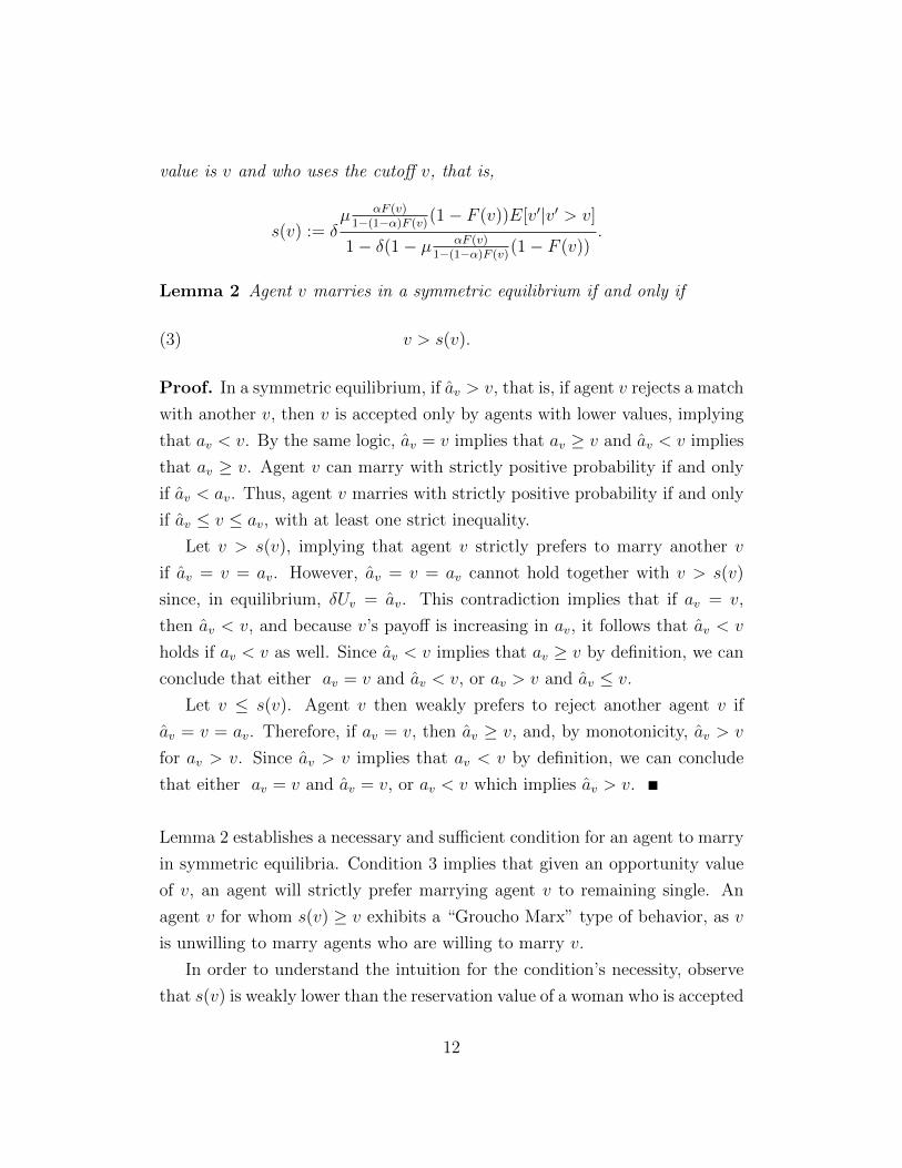
value is v and who uses the cutoff v, that is,
s(v) := δµ αF (v)
1−(1−α)F (v)(1− F (v))E[v′|v′ > v]
1− δ(1− µ αF (v)1−(1−α)F (v)
(1− F (v)).
Lemma 2 Agent v marries in a symmetric equilibrium if and only if
v > s(v).(3)
Proof. In a symmetric equilibrium, if av > v, that is, if agent v rejects a match
with another v, then v is accepted only by agents with lower values, implying
that av < v. By the same logic, av = v implies that av ≥ v and av < v implies
that av ≥ v. Agent v can marry with strictly positive probability if and only
if av < av. Thus, agent v marries with strictly positive probability if and only
if av ≤ v ≤ av, with at least one strict inequality.
Let v > s(v), implying that agent v strictly prefers to marry another v
if av = v = av. However, av = v = av cannot hold together with v > s(v)
since, in equilibrium, δUv = av. This contradiction implies that if av = v,
then av < v, and because v’s payoff is increasing in av, it follows that av < v
holds if av < v as well. Since av < v implies that av ≥ v by definition, we can
conclude that either av = v and av < v, or av > v and av ≤ v.
Let v ≤ s(v). Agent v then weakly prefers to reject another agent v if
av = v = av. Therefore, if av = v, then av ≥ v, and, by monotonicity, av > v
for av > v. Since av > v implies that av < v by definition, we can conclude
that either av = v and av = v, or av < v which implies av > v.
Lemma 2 establishes a necessary and sufficient condition for an agent to marry
in symmetric equilibria. Condition 3 implies that given an opportunity value
of v, an agent will strictly prefer marrying agent v to remaining single. An
agent v for whom s(v) ≥ v exhibits a “Groucho Marx” type of behavior, as v
is unwilling to marry agents who are willing to marry v.
In order to understand the intuition for the condition’s necessity, observe
that s(v) is weakly lower than the reservation value of a woman who is accepted
12

by men whose value is lower than v and rejected by men whose value is greater
than v. By the monotonicity of the reservation values, whenever man v is
willing to marry woman w, her reservation value is weakly greater than s(v).
Hence, when s(v) > v, woman w prefers remaining single to marrying v and
so v cannot marry in equilibrium.11
To see why Condition 3 is also sufficient, note that in a symmetric equilib-
rium, v will not marry only if all agents whose value is greater than v reject
v (i.e., av ≤ v). Agent v’s reservation value increases in av and so, if v > s(v)
and av ≤ v, then agent v accepts agents whose value is lower than v. As the
agents’ reservation values are monotone in their values, all agents whose value
is lower than v accept v and so v marries in a symmetric equilibrium.
Condition 3 allows us to understand who will marry in equilibrium. As
s(v) is continuous and s(v) = s(v) = 0, agents with extreme match values
always marry in equilibrium while agents with intermediate match values may
search indefinitely. We now use Condition 3 to study the effect of the matching
frictions, µ and δ, and the feedback parameter α on the share of eternal singles
in a symmetric equilibrium.
Proposition 3 The share of agents who never marry in a symmetric equilib-
rium weakly increases in δ, µ, and α. Moreover, for any α and µ, this share
converges to 1 as δ converges to 1.
Proof. We can write Condition (3) as
1− δδ
v > µαF (v)(1− F (v))
1− (1− α)F (v)E[v′ − v|v′ > v].(4)
Note that an agent for whom (4) does not hold cannot marry in equilibrium.
The LHS of (4) is decreasing in δ and so every agent who cannot marry in
equilibrium under δ cannot do so under any δ′ > δ. Moreover, at the δ = 1
limit, the LHS of (4) goes to 0 such that (4) cannot hold for v ∈ (v, v). Clearly,
the RHS of (4) is increasing in µ and α, which completes the proof.
11When s(v) > v, agent v cannot marry regardless of whether the equilibrium is symmetricor not.
13

Proposition 3 establishes that the share of eternal singles increases when search
frictions vanish and as agents’ obtain better feedback on matches they reject.
What makes the agents so selective when the search frictions vanish? To
understand the intuition, consider an agent v who marries in equilibrium.
Agent v is accepted by (at least) all agents with a value lower than v. No
matter what cutoff strategy v uses, v believes that (s)he will be accepted by
every agent with a probability weakly higher than αF (v). As search frictions
vanish, v expects to encounter more and more agents with high match values
and, therefore, v will never accept an agent of her/his own caliber.
In order to understand the effect of the feedback parameter α, note that
an agent v who marries in equilibrium is accepted by every agent whom v
rejects. The higher α is, the higher agent v’s perceived probability βv is, as v
obtains more “positive feedback” from matches v rejects. When v’s perceived
probability increases, v becomes more selective to the extent that, for large
values of βv, agent v is too selective to marry.
3.3 Overoptimism and Oversearch
In the previous section, we established that some agents in our model may
search indefinitely and never leave the market. This suggests that, in general,
agents may be too selective and search longer than optimal. We now show
that this is indeed the case. While agents who are accepted by everyone are
correct in their predictions and behave as if they were fully rational, all other
agents overvalue their prospects in the market and continue their search longer
than optimal.
Proposition 4 There exists a value v1 < v such that every agent v ≥ v1
behaves as if (s)he were fully rational and every agent v < v1 searches longer
than optimal. Moreover, [v1, v] is the top class in Proposition 1.
Proof. First, consider the agents’ perceived probability of marriage in each
period. Agent v expects to accept a match with probability 1− F (av) and to
14

be accepted in each period with probability
βv =
F (av)−F (av)+αF (av)
1−F (av)+αF (av), if av ≥ av
αF (av)1−F (av)+αF (av)
, if av < av.
The correct probability with which agent v is accepted, conditional on v
accepting, is
max{F (av)− F (av), 0}1− F (av)
,(5)
which is lower than βv unless av = v or av = v.
Second, consider the agents’ expected value from marriage. Agent v marries
an agent whose expected value is E[v′|av ≤ v′ < av] but believes that (s)he
will marry an agent whose expected value is E[v′|av ≤ v′ ≤ v]. The latter
value is higher, unless av = v.
Therefore, unless av = v, in which case the agent is correct and behaves
optimally, agent v’s perceived expected payoff, Uv, is higher than the actual
one. Hence, the agent’s cutoff value, av, is too high as well, since av = δUv.
This means that the agent searches longer than optimal, given av.
Lastly, note that due to search frictions, there must be agents who are
accepted by all other agents. By the monotonicity of av, there exists a value
v1 such that av = v for v ≥ v1 and av < v for v < v1.
Agents who are accepted by all other agents behave as if they were fully
rational. They correctly predict the time it will take them to marry and
their partner’s expected value. The reason that these agents are unaffected
by selection neglect is that for these agents, there is no selection, namely, all
other agents are equally (non)selective with regard to these agents.
All other agents are affected by their neglect of the fact that agents who are
more valued are also more selective. There are two reasons why this neglect
can make agents search longer than optimal: overestimation of the expected
value of their potential partner in a future marriage and underestimation of
the time it will take them to get married.
15

Agents overestimate the expected value of their potential partner because
they believe that all agents are equally achievable and, therefore, they believe
that they are equally likely to marry any agent whom they accept. However,
since agents who are more valued are also more selective, agents either re-
main single forever or marry an agent whose expected value is lower than the
expected value of the matches they accept.
Agents underestimate the time it takes them to get married since they
overestimate the rate of a mutual match acceptance. Recall that our agents
average over all possible partners when they form expectations (on the rate
at which others find them acceptable). They mistakenly include potential
partners that they themselves reject but are accepted by, which raises the
acceptance rate. Our agents also mistakenly include agents they accept but
are rejected by, which lowers the acceptance rate. It turns out that the more
dominant mistake is the first. Hence, our agents include too many observations
in which they are accepted, which induces overestimation of the probability of
marriage in each period.12
3.4 Characterization and Existence
In this section, we focus on the structure and existence of the equilibria of
the model. We construct a symmetric equilibrium in which there is block
segregation. The construction shows that, in general, there are an infinite
number of such equilibria but, by Condition 3, the set of agents who marry
in equilibrium is unique. We conclude this section by relaxing the symmetry
assumption and illustrating the structure and properties of such equilibria.
In constructing the symmetric equilibria, we use the fact that Condition 3
allows us to partition [v, v] into maximal intervals in which either all agents
marry (marriage intervals) or none do (singles intervals). We treat each interval
separately and partition them into a potentially infinite number of classes, in
which all agents share the same reservation and opportunity values.
As in the rational case, a top class exists and it is possible to construct
12When av = v, agent v correctly predicts the time it will take her/him to marry as thereis no selection along this dimension.
16

a sequence of classes that starts from it. However, unlike in the rational
case (unless δ is sufficiently small), the sequence will not cover [v, v] and will
converge to the highest value v? such that s(v?) = v? instead. That is, the
classes cover only the top marriage interval.
The main challenge in the proof is that, unlike in the top marriage interval
(and unlike in the rational case), in any other interval there is no upper class
from which we can start the construction. Nevertheless, we show that it is
possible to define an arbitrary initial class in the interior of each of these
intervals and construct two unique sequences of classes on each of the initial
class’ sides. The sequences cover the interval and converge to its end points.
Such freedom in defining the initial class implies that there are an infinite
number of equilibria once the partition includes more than one interval. There
is no such freedom in the top marriage interval (or in the rational expectations
model) due to the uniqueness of the upper class.
Formally, by Condition 3, we know that one can partition [v, v] into maxi-
mal intervals in which agents either eventually marry or remain single forever.
We say that L is a marriage interval, if L is a maximal interval such that
s(l) < l for all l ∈ L. An interval L is said to be a singles interval if either
s(l) > l for all l ∈ L, or s(l) = l for all l ∈ L. In the latter case, L is often a
singleton. Denote [l, l] := cl(L).
We say that C = [c, c] is a class if either C = cl({v|av = c}) = cl({v|av =
c}) or C = cl({v|av = c}) = cl({v|av = c}). Thus, in each class, the agents
share identical cutoff rules and opportunity values. We refer to classes con-
tained in marriage intervals as marriage classes and to classes contained in
singles intervals as singles classes.
The following lemma is key in establishing that, in equilibrium, if an in-
terval L contains one class, then L is covered by classes.
Lemma 3 In equilibrium, if an interval L contains a class C, then (i) L
contains a unique class C ′ such that c = c′, unless c = v, and (ii) L contains
a unique class C ′′ such that c′′ = c, unless c = v.
Proof. Assume that C is a marriage class and c 6= v. By the definition of a
17

class, for any agent v > c, av ≥ c. Since C is in a marriage interval, limv→c+
av = c.
There exists a unique value ac > c such that limv→c+
av = ac for which limv→c+
av = c
is optimal. By the definition of ac and monotonicity, av = c for any v ∈ (c, ac).
This implies that av = ac for all such v. Therefore, C ′ = [c, ac] is a class.
Assume that C is a singles class and c 6= v. For any v > c, av ≥ c. Since
C is in a singles interval, limv→c+
av = c. There exists a unique value ac > c
such that limv→c+
av = ac is optimal given limv→c+
av = c. By the definition of ac,
av = c for any v ∈ (c, ac). This implies that av = ac for all such v. Therefore,
C ′ = [c, ac] is a class.
The proofs for the existence of C ′′ follow the same logic and are omitted
for brevity.
By Lemma 3, if an interval L contains a finite number of classes, then
L = [v, v]. Moreover, an infinite sequence of classes must converge to some v
satisfying s(v) = v. Thus, if cl(L) = [l, l] then either l = v or s(l) = l, and
either l = v or s(l) = l. The next corollary follows immediately.
Corollary 1 If an interval L contains one class, then L is covered by classes.
In equilibrium, there must be two sets of agents, one on each side of the
market, who are accepted by all the other agents. The set of agents who are
accepted by all the other agents on one side of the market must have a common
cutoff strategy, i.e., a joint av, which, in turn, defines the set of agents who are
accepted by all the other agents on the other side of the market. These two sets
of agents are uniquely determined by the distribution F . Thus, Proposition 4
and Corollary 1 imply the following Corollary.
Corollary 2 In equilibrium, the highest marriage interval is covered by classes
in a unique manner.
If δ is sufficiently low such that s(v) > v for all v, implying that all
agents marry in equilibrium, then Corollary 2 establishes that the equilibrium
is unique. Otherwise, the equilibrium is uniquely defined over the highest
marriage interval.
18

In the following proposition, we show, by construction, that an equilibrium
exists. This is established by defining an arbitrary class in each interval (except
the highest) and then covering each interval with additional classes.13 This
construction highlights the fact that the equilibrium is not unique whenever
there is more than one interval. Nonetheless, the set of agents who remain
single in equilibrium is unique.
Proposition 5 A symmetric equilibrium exists.
Proof. For any point v for which s(v) = v, set av. The following construction
will ensure that av = v as well. By definition, av = v is optimal given av = v.
In the remainder of the proof, singles intervals are assumed to contain only
agents with s(v) > v.
Let L be a maximal interval that does not contain v or v, and let a ∈ int(L)
and ε ∈ R. Define v = a+ε. Consider v’s discounted payoff, δUv, as a function
of ε, assuming that av = v and av = a. If L is a marriage interval, then for
ε = 0, δUv < v. For ε = l − a, δUv > l = v ( l’s payoff when al = al = l is l).
If L is a singles interval, then for ε = 0, δUv > v. For ε = l − a, δUv < l = v
( l’s payoff given al = al = l is l). In either case, the payoff is continuous in ε
and, therefore, for some ε, δUv = v. Note that v ∈ L.
Consider now the dual exercise: let L be a maximal interval that does not
contain v or v, and let w ∈ L. If L is a marriage interval, consider a ∈ [w, l]
and find a v as in the previous paragraph. For a = w, v < w. For a = l,
v = l > w. If L is a singles interval, consider a ∈ [l, w] and find a v as in the
previous paragraph. For a = w, v > w. For a = l, v = l < w. In either case,
by continuity, there exists an a such that v = w. Note that a ∈ L.
Thus, given any v ∈ L we can find an interval [v, a] ∈ L, such that v is
the optimal cutoff given a, and an interval [a, v] ∈ L, such that a is optimal
given v. Arguments for the existence of an interval of the first type for L not
containing v and an interval of the second type for L not containing v are
similar and omitted for brevity.
13It is also possible to construct equilibria with no classes, except in the highest interval.
19

Let L be a maximal interval that does not contain v or v, and let c0 ∈int(L). For k = 1, 2, ..., let ck be the value for which δUv = ck−1 if av = ck−1
and av = ck. For l = 1, 2, ..., let cl be the value for which δUv = c−l if av = l−l
and av = c1−l. Note that both series {ck}k∈N and {cl}l∈N are bounded by
L and monotonic, and hence converging. At the limit, v, it must hold that
v = av = av. Thus, v ∈ {l, l}. For k ∈ Z, define Ck = [ck, ck+1). Note that the
sets {Ck}k∈Z are disjoint and cover int(L). Set av = ck for any v ∈ [ck, ck+1),
al = l, and al = l
Let L be a maximal interval containing v. Set c0 = v. For any l = 1, 2, ...,
let cl be the value for which δUv = cl−1 if av = c−l and av = c1−l. In the case of
c−l ≤ v, set c−l = v and stop the process. Define C l = [cl, cl+1) for l = 1, 2, ...
. As in the previous case, the sets {C−l}l∈N are disjoint and cover int(L). Set
av = c−l for any v ∈ [c−l, c1−l) and av = c−1.
Let L be a maximal interval containing v but not v. Set c0 = v. For any
k = 1, 2, ..., let ck be the value for which δUv = ck−1 if av = ck−1 and av = ck.
Define Ck−1 = [ck−1, ck] for any k = 1, 2... . Set av = c−1 for any v ∈ [ck−1, ck)
and av = c0.
By construction, for any v in any interval L, if av = ck for some k, then
av = ck+1. Furthermore, this av is optimal given av. Thus, an equilibrium
exists.
To conclude, the following proposition summarizes our results:
Proposition 6 Fix µ and α. There exists δ such that:
1. If δ ≥ δ, then (i) there exist an infinite number of symmetric equilibria,
and (ii) there is a set of agents with intermediate match values who do
not marry in any equilibrium.
2. If δ < δ, then (i) there exists a unique equilibrium and (ii) all agents
marry in equilibrium.
For every δ, there exists a top class, C0, that is identical to C0 in the benchmark
case of Proposition 1.
20

Comment: Symmetry in the model
Throughout the analysis, we imposed symmetry along two dimensions: we
focused on symmetric equilibria and assumed that the men’s and women’s
values are drawn from identical distributions. These assumptions allowed us
to convey the main messages while keeping the exposition simple. However,
our key insights are not sensitive to these assumptions. Since the implications
of both types of asymmetry are similar, we focus our discussion on the case
where the distributions of values are symmetric but the equilibrium is not.
The condition s(v) ≤ v remains necessary for marriage as, if s(v) > v and
man (woman) v accepts a match with woman (man) w, then all men (women)
whose value is lower than v accept w and so w rejects the match with v.
Moreover, as Proposition 3 shows, s(v) increases in δ, µ, and α. Thus, the key
insights of the paper remain valid.
The main change when we relax the symmetry assumption is that Condi-
tion 3 is no longer sufficient for marriage. As an illustration, let F be such
that s(v) = v for some v and denote that lowest such v by v?. Construct a
symmetric equilibrium as in Proposition 5 and make the following two mod-
ifications: set av = v? for all women with v ∈ [v, v?] and av = v for all men
with v ∈ [v, v?]. Note that (1) av = v? for all women with v ∈ [v, v?], which
implies that av = v? is optimal for these women and (2) av = v for all men
with v ∈ [v, v?], which implies that av = v is optimal for these men. For all
other agents, the opportunity and reservation values remain as in Proposition
5 and so the profile we described is an equilibrium in which low-valued agents
never marry (unlike in a symmetric equilibrium, in which low-valued agents
do marry).
The equilibrium we constructed highlights a general property: in a sym-
metric equilibrium, agents are partitioned into marriage and singles intervals,
based on whether s(v) ≥ v or s(v) < v in each interval. In an asymmetric
equilibrium, it is possible to turn every marriage interval into a singles inter-
val, except for the top marriage interval. Agents in that interval behave as in
a symmetric equilibrium (as Corollary 2 still applies and these agents’ behav-
ior is pinned down by the top class). Thus, the set of agents who marry in a
21

symmetric equilibrium is a superset of the agents who marry in an asymmetric
equilibrium.
4 Extensions
In this section, we modify the baseline model along two dimensions and ex-
amine the implications for our results. First, we consider a model in which
one side of the market consists of fully rational agents while agents on the
other side of the market are boundedly rational. We show that the existence
of the fully rational agents can lead to unraveling. We then focus on a case
where agents obtain no feedback from matches they reject and show that, as in
the previous sections, agents overestimate the value of their potential partner.
However, they do not underestimate the time it will take them to marry. As
a result, agents search longer than optimal but eventually all of them marry.
4.1 One-Sided Full Rationality
Consider a case in which agents on one side of the market are fully rational,
while on the other side of the market the agents’ reasoning is coarse. This
setting corresponds to hiring situations, where workers might be partially so-
phisticated while firms invest more resources in gathering information and
analyzing the market.
A natural question is whether the existence of the fully rational agents on
one side of the market alleviates the problem of oversearch or not. The next
result shows that not only is the answer to this question negative, but, in
fact, the share of eternal singles is greater when one side of the market is fully
rational.
Proposition 7 Suppose that every v ∈ W is fully rational and assume that
s(v?) > v? for some v? < v. In equilibrium, all women whose value is lower
than v? never marry.
Proof. Observe that Lemma 1 still applies (to both sides of the market).
Consider woman v?. If she accepts a man v, then every woman whose value
22

is lower than v? accepts man v and so δUv ≥ s(v?) > v?. Thus, man v rejects
woman v?. It follows that woman v? cannot marry in equilibrium. Hence,
no man ever accepts woman v?, as otherwise she could deviate to accept that
man. By monotonicity, no man ever accepts a woman w < v?.
Proposition 7 shows that even rational agents who are fully aware of the bound-
edly rational agents’ overselectiveness may find themselves forever single. In
fact, compared to the case where W contains boundedly rational agents, fewer
women marry when all women are fully rational (as, when women are only par-
tially sophisticated, women at the bottom of the value distribution do marry).
The intuition for Proposition 7 is as follows. Fully rational agents react
to the overselectiveness of agents on the other side of the market by lowering
their own standards. If agents of their own caliber reject them, they turn
to lower-valued agents (unlike boundedly rational agents who do not expect
difficulty in matching with agents of their own caliber). The fully rational
agents’ lower standards raise the standards of lower-valued boundedly rational
agents, thereby exacerbating the problem: the low-valued boundedly rational
agents become even more overoptimistic as they are accepted by higher-valued
rational agents and refuse to marry these agents as well. This process leads to
unraveling as, eventually, higher-valued women will accept all men while even
the lowest-valued man will be unwilling to marry them.
4.2 No Feedback from Rejected Matches (α = 0)
Our agents estimate the acceptance likelihood of a potential match by observ-
ing, and averaging over, agents they both reject and accept. In this section, we
consider the extreme case in which agents do not observe whether agents they
reject accept them or not. In other words, agents form their expectation solely
by observing the acceptance rate of agents they accept themselves. Formally,
in this section we assume that α = 0. Thus,
βv =
∫Av(σ)∩Av(σ)
f(x)dx∫Av(σ)
f(x)dx=max{F (av)− F (av), 0}
1− F (av).(6)
23

Note that βv is the correct average probability that agents whom v finds
acceptable accept v in return. Thus, there is no selection neglect along the
probability dimension.
At this point, a conceptual issue may arise: how should an agent form a
belief about the behavior of agents they reject and never observe? We follow
the leading example in Esponda (2008) and assume that agents extrapolate
from the data they do observe in equilibrium and believe that the agents they
reject find them acceptable with probability14 βv.
An agent who marries in equilibrium, has a perceived expected payoff of
Uv =µ[F (av)− F (av)]E[v′|v′ ≥ v]
1− δ(1− µ[F (av)− F (av)]).(7)
When α = 0, agents may still overestimate the value of a potential marriage
as they think that other agents are equally achievable. The selection neglect
along the value dimension makes them overselective and leads them to search
longer than optimal.
An agent who does not marry in equilibrium obtains a correct perceived
payoff of 0. The next result shows that this cannot happen in equilibrium: even
though most agents suffer from selection neglect, overvalue the prospect of
remaining single, and search longer than optimal, all agents eventually marry
and there is block segregation.
Proposition 8 Fix α = 0. There exists a unique equilibrium in which all
agents marry and the block segregation result holds. In this equilibrium, there
is a value v1 < v such that every agent v ≥ v1 behaves as if (s)he were fully
rational and every agent v < v1 searches longer than optimal.
The proof of Proposition 8 is by construction and follows the same logic
as in previous proofs: there exists a unique upper class (identical for any α).
Additional classes are then constructed in a unique manner. As the proof
follows directly from Corollary 2, it is omitted.
14Our subsequent results do not rely on this assumption.
24

The key difference between the case of α = 0 and that of α > 0 is the lack
of eternal singles in the former case. When there is no selection neglect along
the probability dimension, if there were an “eternal single” v, then v would
conclude that (s)he will marry with probability 0. Thus, v would adjust av to
v and accept matches with all agents, which would lead v to marry.
5 Concluding Remarks
We studied a model of two-sided search with nontransferable utility and agents
who use a coarse model of the world to assess their prospects. We found that
the most desirable agents behave as if they were fully rational while all the
other agents overvalue the option of remaining single. This problem is most
severe for agents with intermediate match values, who, if the search frictions
are not too intense, search indefinitely.
Throughout the analysis we assumed that agents who marry obtain the
value of their spouse or, in Burdett and Coles’ (1997) words, “Looking in the
mirror to admire one’s own pizzazz does not increase utility.” While this is
natural in some contexts, there is some complementarity between partners in
other contexts. The main results and intuitions of the paper hold in some set-
tings in which partners complement each other (e.g., when the payoff function
is multiplicatively separable, as analyzed in Eeckhout, 1999). In fact, as long
as agents who are more valued are also more selective (which is necessary in
any form of assortative mating) our qualitative results hold.15
A key insight of this paper is that when agents are not fully rational, tech-
nological advancement that thickens markets and allows agents to search faster
can make them worse off. The improvements in the search technology exac-
erbate the agents’ biases and increase their overselectiveness. This insight is
particularly important in designing modern search environments where agents
may be overwhelmed by the wide variety of possibilities, which can lead them
to use simplified models of the world.
15To see this, note that the structure of Condition 3, which is the cornerstone of ouranalysis, depends only on the monotonicity of the agents’ reservation values.
25

References
[1] Adachi, H. (2003): “A Search Model of Two-Sided Matching under Non-
transferable Utility,” Journal of Economic Theory, 113, 182–198.
[2] Antler, Y. (2015): “Two-Sided Matching with Endogenous Preferences,”
American Economic Journal: Microeconomics, 7, 241–258.
[3] Benabou, R. (2015): “The Economics of Motivated Beliefs,” Revue
d’Economie Politique, 125, 665–685.
[4] Bloch, F. and Ryder, H. (2000): “Two-Sided Search, Marriages, and
Matchmakers,” International Economic Review, 41, 93–116.
[5] Bruch, E. and Newman, M. (2018): “Aspirational Pursuit of Mates in
Online Dating Markets,” Science Advances, 4, eaap9815.
[6] Burdett, K. and Coles, M. (1997): “Marriage and Class,” Quarterly Jour-
nal of Economics, 112, 141–168.
[7] Chade, H. (2001): “Two-Sided Search and Perfect Segregation with Fixed
Search Costs,” Mathematical Social Sciences, 42, 31–51.
[8] Chade, H. (2006): “Matching with Noise and the Acceptance Curse,”
Journal of Economic Theory, 129, 81–113.
[9] Chade, H., Eeckhout, J., and Smith, L. (2017): “Sorting through Search
and Matching Models in Economics,” Journal of Economic Literature, 55,
493–544.
[10] Eeckhout, J. (1999): “Bilateral Search and Vertical Heterogeneity,” In-
ternational Economic Review, 40, 869–887.
[11] Eliaz, K. and Spiegler, R. (2013): “Reference Dependence and Labor
Market Fluctuations,” NBER Macroeconomics Annual, 28, 159–200.
[12] Enke, B. and Zimmermann, F. (2017): “Neglect in Belief Formation,”
Review of Economic Studies, 86, 313–332.
26
[13] Eyster, E. and Rabin, M. (2005): “Cursed Equilibrium,” Econometrica,
73, 1623–1672.
[14] Francesconi, M. and Lenton, A. (2012): “Too Much of a Good Thing?
Variety Is Confusing in Mate Choice,” Biology Letters, 7, 528–31.
[15] Gamp, T. and Krahmer, D. (2019a): “Cursed Beliefs in Search Markets,”
Mimeo.
[16] Gamp, T. and Krahmer, D. (2019b): “Deception and Competition in
Search Markets,” Mimeo.
[17] Hinge (2016): ”The Dating Apocalypse,” retrieved from
https://thedatingapocalypse.com/stats/.
[18] Jehiel, P. (2005): “Analogy-Based Expectation Equilibrium,” Journal of
Economic Theory, 123, 81–104.
[19] Jehiel, P. (2018): “Investment Strategy and Selection Bias: An Equilib-
rium Perspective on Overoptimism,” American Economic Review, 108,
1582–1597.
[20] MacNamara, J. and Collins, E. (1990): “The Job Search Problem as an
Employer-Candidate Game,” Journal of Applied Probability, 28, 815–827.
[21] Pew Research Center (2016): “5 Facts about Online Dating,” retrieved
from https://www.pewresearch.org/fact-tank/2016/02/29/5-facts-about-
online-dating/.
[22] Piccione, M. and Rubinstein, A. (2003): “Modeling the Economic Interac-
tion of Agents with Diverse Abilities to Recognize Equilibrium Patterns,”
Journal of the European Economic Association, 1, 212–223.
[23] Spiegler, R. (2019): Behavioral Implications of Causal Misperceptions,
Mimeo.
[24] Shimer, R. and Smith, L. (2000): “Assortative Matching and Search,”
Econometrica, 68, 343–369.
27

[25] Smith, L. (2006): “The Marriage Model with Search Frictions,” Journal
of Political Economy, 114, 1124–1146.
28