Embed Size (px)
Citation preview
20 February 2014
Literature Thesis
Sedimentation Velocity Analytical Ultracentrifugation
(SV-AUC) for characterizing protein aggregates and
contaminants in therapeutic proteins
The elaboration of mathematical relations behind SV-AUC theory
AUTHOR(S) : Lam, S.
SUPERVISORS : dr. W. Th.Kok (Universiteit van Amsterdam)

Literature thesis S. Lam
2

Literature thesis S. Lam
3
MSc Chemistry
Analytical Sciences
Literature Thesis
Sedimentation Velocity Analytical Ultracentrifugation
(SV-AUC) for characterizing protein aggregates and
contaminants in therapeutic proteins
The elaboration of mathematical relations behind SV-AUC theory
by
S. Lam
February 2014
Supervisor:
dr. W.Th. Kok

Literature thesis S. Lam
4

Literature thesis S. Lam
5
Table of context
Table of context 5
Abstract 6
1. Introduction 7
2. Protein aggregates and contaminants 9
3. Sedimentation Velocity Analytical UltraCentrifuge (SV-AUC) 11
3.1 Sedimentation velocity versus sedimentation equilibrium 11
3.2 Principle of the AUC 12
3.3 Principle of sedimentation boundary modeling (Lamm equation) 16
3.4 Sedimentation coefficient 18
3.5 Apparent sedimentation coefficient 18
4. Instrumentation 20
4.1 Analytical ultracentrifuge 20
4.2 XLA 23
4.3 XLI 24
4.4 Ordering 24
4.5 Application of the AUC 25
5. Analyses and approach 26
5.1 Apparent sedimentation coefficient distribution g*(s) analysis 26
5.2 Sedimentation coefficient distribution c(s) analysis 27
5.3 Therapeutic product related impurities (contaminations) 28
5.4 Approach and interpretation of the applications 28
6. Applications 31
6.1 Comparison between c(s) and g(s*) analyses 31
6.2 c(s) distribution with low aggregation levels 32
6.3 Therapeutic monoclonal antibodies homogeneity 33
6.4 Fluorescence detection 35
7. Conclusion 36
8. Discussion 36
References 37
Literature thesis S. Lam
6
Abstract
Sedimentation velocity analytical ultracentrifugation (SV-AUC) is one of the classical
techniques for the study of protein aggregates and contaminations in therapeutic drugs (i.e.
monoclonal antibodies). Monitoring the sedimentation of proteins in the centrifugal field
allows the characterization of the sedimentation behavior of the particles in the solution,
without any interaction with matrix or surface. The sedimentation behavior and the rate of
sedimentation are described by the sedimentation velocity (SV) analysis.
The current thesis focuses mainly on the determination of the homogeneity and the
detection of small levels of soluble species (e.g. dimer, trimer, and so on). However, the
overload of new advancements, complex computational theories and large data sets make it
difficult for the protein scientists to gain sufficient expertise to apply AUC to their research
problems. Therefore, this thesis will initially explain the basic principle of SV-AUC, followed
by the modeling of the sedimentation boundaries obtained with this technique.
The two modeling analyses c(s) and g(s*) supported by the computational programs SEDFIT
and DCDT+, respectively, provide (apparent) sedimentation coefficient distributions. These
distributions are similar to chromatograms and are therefore easily to be interpreted.
However, c(s) and g(s*) analyses are slightly different, because c(s) includes diffusion while
g(s*) does not. After comparison, c(s) analysis was selected to continue with other
measurements, because it has a more improved resolution and sensitivity compared to g(s*)
analysis.
SV-AUC using c(s) analysis enables to determine the homogeneity of different types of
therapeutic proteins. It is also possible to detect small aggregates at low concentration levels.
A breakthrough for this SV-AUC will be the incorporation of the fluorescence detection into
account next to the currently used absorbance and interference detection, because the
sensitivity of fluorescence detection is much higher. This makes detecting low concentrated
aggregates and contaminants in strongly diluted samples possible.

Literature thesis S. Lam
7
1. Introduction
In pharmaceutical chemistry studies, proteins (e.g. monoclonal antibodies[ 1 ]) are an
important division of therapeutic drugs[2]. In order to obtain therapeutic drugs, complex
reaction mechanisms are generally carried out between proteins from a particular biological
mixture. However, the same proteins can appear in different forms (e.g. misfolded,
denaturated and degraded) because the weak interactions and disulfide bonds that hold the
sensitive protein molecules together can be easily disrupted by stresses during purification,
storage or processing. The stresses[3] can be caused by several factors such as: hydrophobic
surfaces, elevated temperature, a change in pH, high shear, (hydrophobic) surface
adsorption, and the removal of water and high protein concentrations.
In general, a structural alteration in protein's structures often leads to protein
aggregation[1],[2],[4]. Protein aggregation is related to protein physical degradation and a
decrease of immunogenicity[2],[5],[6]. Therefore protein aggregates can have a negative
influence on the therapeutic drugs and also activate adverse resistant reactions to the drug.
Due to the complexity of protein's characteristics (i.e. various reactive chemical groups and
weak three-dimensional structures), it is however, practically impossible to develop a
therapeutic drug consisting of solely a pure native form of the protein.
In clinical research, maintaining the appropriate efficacy and safety of the therapeutic drug
ensures the quality of the therapeutic product. Because there are no clear guidelines or
agreed-upon approach in pharmacopoeia to ensure the quality[4] of the product. It is
imperative to have a control of the amount of protein aggregates, contamination and
homogeneity of the therapeutic protein. Consequently, characterization and identification
of protein aggregates and contaminants of the product is essential to eventually understand
the degradation pathways affecting proteins and the goal of an extensive repertoire of
analytical methods. Once the degradation pathways are discovered, the quality of the
therapeutic drug can be improved. Furthermore, therapeutic products are often
contaminated with host-cell-protein or non-protein particles besides the protein aggregates,
such as silica particles and leachates. These contaminations can lead to an expansion of
protein aggregates, which results in a serious damage to the product.
Moreover, protein aggregation has become a significant problem in the biopharmaceutical
industry due to its medical association with over 40 human diseases[7] (e.g. Alzheimer’s,
Parkinson's, Huntington's, prion and type II diabetes). Since protein aggregation has so
much impact on the characteristic of (therapeutic) protein drugs, it is necessary to measure
the amount of protein aggregation and comprehend the nature of protein structures to
understand the protein aggregation conditions.
Literature thesis S. Lam
8
It should be noted that protein aggregates can be divided into different categories according
to solubility, reversibility, size and type of bonding[8]. The details of protein aggregates will
be discussed later in this thesis.
In this literature thesis, the selected analytical technique to characterize, identify and
quantify protein aggregates and contaminants is sedimentation-velocity analytical
ultracentrifugation (SV-AUC[9],[10],[11]). AUC actually has two modes (the sedimentation
velocity and sedimentation equilibrium modes[ 12 ],[ 13 ],[ 14 ]), but in this paper only
sedimentation velocity (SV)[15] measurements will be discussed. SV is more commonly used,
because it is a more time-saving and wider applicable method compared to the
sedimentation equilibrium mode. SV-AUC is selected to determine protein aggregation and
contaminants in therapeutic products because 1) SV-AUC has a typically measuring size
range[16] of 1.0 nm - 110 nm for protein aggregates, monomers and oligomers and 2) sample
destruction is not necessary due to its matrix- and column-free approach. The principle,
applicability and performance of SV will be discussed in chapters 2 and 3.
The SV-AUC is able to provide extension information on protein aggregates and
contaminants when supported by complex computational and internet resources. The
corresponding software programs SEDFIT[17] and DCDT+[22] are used to model sedimentation
data. Boundary modeling of the data based on non-linear least-squares regression includes
the mathematical relations of Lamm's equation[18],[19],[20] (transport-differentiation) and
Stafford[21] (time-derivative[22],[23]) method. Additionally, the two size distribution analyses
that will be discussed and partly compared in this paper are: 1) continuous sedimentation
coefficient distribution c(s) Lamm equation model (using SEDFIT program) and 2) apparent
sedimentation coefficient distribution[20] g*(s) (using DCDT + program).
The complex computational theories make it extremely difficult for protein (bio)scientists to
gain sufficient expertise to apply this modern technique to their research problem and to
manage the interpretation of the measured results. Therefore, this thesis will first explore
the (underlying) mathematical theory behind the SV-AUC to gain more knowledge of the
application of this analytical technique.
The major aim of this paper is to gain a greater understanding of the difficult mathematical
relation and principle of SV-AUC for the characterization of protein aggregates and
contaminations in therapeutic drugs. The methodology of SV-AUC is certainly not trivial,
because this can provide sufficient information to assist protein scientists to link with
different type of research with respect to therapeutic drugs, proteins, protein complexes
and protein aggregates.
Literature thesis S. Lam
9
2. Protein aggregates and contaminants
When a protein binds to other copies of the same molecule they can oligomerize[24]. This
chemical process occurs between a few monomers and forms dimers, trimers or tetramers.
As the composition has exceeded four monomers, oligomer becomes polymer.
The advantageous feature to explore protein oligomerization is that due to these subunits
interactions the activity of the protein becomes concentration dependent and is therefore
beneficial for functional control. Proteins are not only occupied with self-associated
interactions[24], but also hetero-associated interactions[25],[26]. The latter occurs when the
protein interacts with other molecules. If protein interacts with other protein it forms a
protein complex[27] and is considered as a protein interacting system. The interactions
between two different proteins play an important role in various diseases.
Therapeutic drugs composed of protein mixtures are considered as an increasingly medically
important class because they are associated with over 40 human diseases (e.g. Alzheimer,
Parkinson etc.). Due to the sensitive bindings of proteins, they can be easily influenced by
stress factors. The stress factors (i.e. hydrophobic surfaces, elevated temperature, a change
in pH, high shear, surface adsorption, the removal of water and high protein concentrations)
interfere the protein structures and result unfolding or misfolding of the protein. This
occurrence of protein physical degradation regularly appears in therapeutic proteins.
Structurally changing of proteins forms cause a strong tendency of the protein to aggregate
during storage, processing and manufacturing. Protein aggregation has become a major
concern in pharmaceutical industry over the last decades, mainly due to unclear guidelines
or agree-upon approach in pharmacopoeia. Therefore it is crucial to characterize, quantify
and identify protein aggregates in therapeutic drugs.
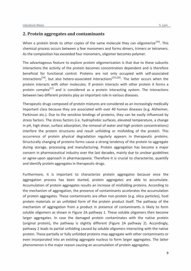
Furthermore, it is important to characterize protein aggregates because once the
aggregation process has been started, protein aggregates are able to accumulate.
Accumulation of protein aggregates results an increase of misfolding proteins. According to
the mechanism of aggregation, the presence of contaminants accelerates the accumulation
of protein aggregates. These contaminants are often non-protein (e.g. silica particles), host
protein materials or an unfolded form of the protein product itself. The pathway of the
mechanism of aggregation from a product in presence of contaminants is likely to form
soluble oligomers as shown in Figure 2A pathway 1. These soluble oligomers then become
larger aggregates. In case the damaged protein contaminates with the native protein
(original protein), the pathway is slightly different (Figure 2A pathway 2). Accordingly,
pathway 2 leads to partial unfolding caused by soluble oligomers interacting with the native
protein. These partially or fully unfolded proteins may aggregate with other contaminants or
even incorporated into an existing aggregate nucleus to form larger aggregates. The latter
phenomenon is the major reason causing an accumulation of protein aggregates.

Literature thesis S. Lam
10
Chemical modification (e.g. oxidation and deamidation) and stress (e.g. elevated
temperature and shear) are mostly the causes of damaged proteins. Minimizing protein
aggregation from these two mechanisms requires homogeneity in the therapeutic product,
therefore the determination of homogeneity is essential.
Figure 2. The pathway of the mechanism of aggregation from a product in presence of contaminants[2]
A third pathway occurs according to the mechanism of protein aggregation for self-
associating systems, which are dependent on low pH, temperature and solvent composition.
The native antibody is taken as an example for the illustration of the self-associating system
(Figure 2 B). This system refers to the formation of aggregates (oligomers) by native
antibodies. Acid stability takes a major role in aggregation of therapeutic monoclonal
antibodies, because both low-pH elution from a protein-A affinity column and viral
inactivation are involved during the purification process. These processes result in partially
unfolded monomers. The unfolded monomers associate with damaged monomers at low pH
and form protein aggregates.
The content of reversible aggregates changes with the total protein according to the law of
mass action. In principle, reversible aggregates will dissociate completely when the
therapeutic protein will be highly diluted in contrast to irreversible aggregates. These
irreversible oligomers are a concern to the therapeutic protein because they do not
dissociate at high dilution. Moreover, reversible aggregates can easily become irreversible
and thus the self-associating proteins aggregation is another pathway for accumulation. To
prevent the cause of this type of aggregates accumulation by self-associating proteins,
reversible aggregates have to be minimized. Therefore, quantitative determination of
content and characteristics of protein aggregate are required.
Literature thesis S. Lam
11
3. Sedimentation Velocity Analytical UltraCentrifuge (SV-AUC) 3.1 Sedimentation velocity versus sedimentation equilibrium
To explain the basic principle of analytical ultracentrifuge (AUC[28],[29]) it should be noted that
this technique can be divided into two modes of operation: sedimentation equilibrium (SE)
and sedimentation velocity (SV). The former is used to obtain thermodynamic properties and
the latter to obtain hydrodynamic properties. Thermodynamic properties[30] are interesting
for characterization of reversible associations and hydrodynamic properties[35] are more for
general determinations. This thesis only focuses on SV, because this is a faster, more general
and wider applicable method than SE. It is worth noting that it is still often recommended to
carry out sedimentation equilibrium mode to complement SV. Furthermore, SV and SE are
based on the same principle.
The selection of which method (sedimentation velocity or sedimentation equilibrium) is
strongly dependent on the type of interaction (static or dynamic). Static interactions are very
slowly reversible or irreversible, whereas dynamic interactions are rapidly reversible on the
time scale of the experiment. Slowly reversible associations cannot physically separate
different states of association during the whole measurement and are commonly studied by
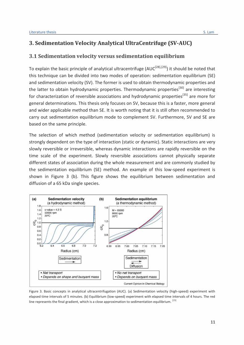
the sedimentation equilibrium (SE) method. An example of this low-speed experiment is
shown in Figure 3 (b). This figure shows the equilibrium between sedimentation and
diffusion of a 65 kDa single species.
Figure 3. Basic concepts in analytical ultracentrifugation (AUC). (a) Sedimentation velocity (high-speed) experiment with
elapsed time intervals of 5 minutes. (b) Equilibrium (low-speed) experiment with elapsed time intervals of 4 hours. The red
line represents the final gradient, which is a close approximation to sedimentation equilibrium. [15]
Literature thesis S. Lam
12
In contrast to dynamic interactions, static associations make it possible to physically
separate and characterize different states of association (e.g. individual oligomers). Static
associations are mostly studied by the sedimentation velocity (SV) method. This method is
shown in Figure 3 (a). Furthermore, the principle of the AUC technique is valid for both SV
and SE methods and will be explained in the next chapter.
3.2 Principle of the AUC
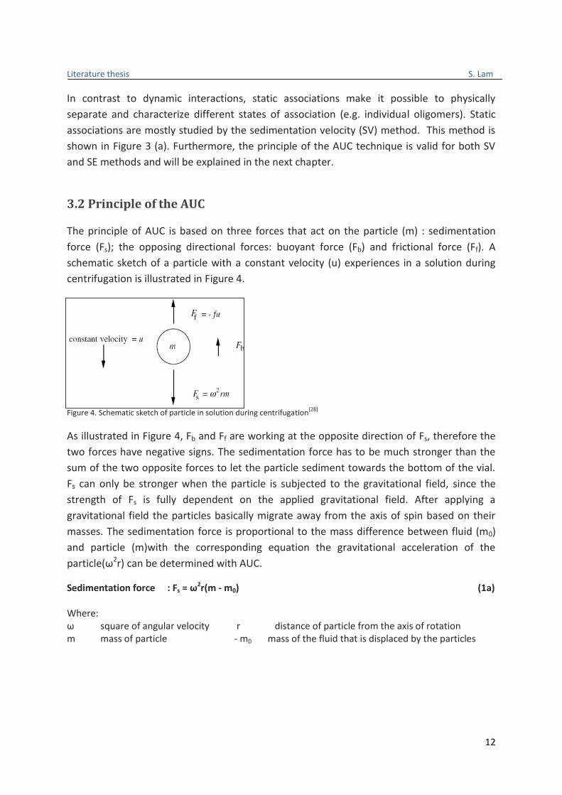
The principle of AUC is based on three forces that act on the particle (m) : sedimentation
force (Fs); the opposing directional forces: buoyant force (Fb) and frictional force (Ff). A
schematic sketch of a particle with a constant velocity (u) experiences in a solution during
centrifugation is illustrated in Figure 4.
Figure 4. Schematic sketch of particle in solution during centrifugation[28]
As illustrated in Figure 4, Fb and Ff are working at the opposite direction of Fs, therefore the
two forces have negative signs. The sedimentation force has to be much stronger than the
sum of the two opposite forces to let the particle sediment towards the bottom of the vial.
Fs can only be stronger when the particle is subjected to the gravitational field, since the
strength of Fs is fully dependent on the applied gravitational field. After applying a
gravitational field the particles basically migrate away from the axis of spin based on their
masses. The sedimentation force is proportional to the mass difference between fluid (m0)
and particle (m)with the corresponding equation the gravitational acceleration of the
particle(ω2r) can be determined with AUC.
Sedimentation force : Fs = ω2r(m - m0) (1a) Where: ω square of angular velocity r distance of particle from the axis of rotation m mass of particle - m0 mass of the fluid that is displaced by the particles
Literature thesis S. Lam
13
The frictional force exists because there is more than one particle in a solution. Basically
when many particles are continuously moving in the solution, the particles are moving along
each other. Thus, it does not matter which direction a specific particle is moving there is
always frictional force between the particles. The corresponding equation for this force:
Frictional force : Ff = -f .u (1b) Where: f frictional coefficient u velocity of the particle
Particles with different sizes sediment with different velocities. The large particles sediment
faster toward the bottom than smaller particles. Additionally, there is a flux diffusion force
or diffusion flux (Jr) that opposes the sedimentation force. Fick's laws of diffusion describe
the movement of the number of molecules from high concentration crossing an area per
time to low concentration regions. The diffusion flux Jr is used to quantify how fast the
diffusion process occurs. The description of diffusion process is described by equation 2a.
Diffusion flux :
(2a)
Where: C Concentration of protein r radius -D diffusion coefficient
The negative sign of the diffusion coefficient (-D) is to cancel the negative concentration
difference, dC (Clow-Chigh), because diffusion occurs from high concentration to low
concentration.
The principle of diffusion flux (force) according to Fick's first law of diffusion is illustrated in
Figure 5A, where the concentration (C) of the particles (y-axis) is plotted against the radius
direction, r-direction (x-axis). The start position (r1, blue dotted line) divides the molecules
into two different (low and high) concentration levels (two solid horizontal lines). Different
end positions are denoted as ri (i = 1, 2,...,n). As two radius positions are selected the radius
and concentration differences, dr (rn -r1) and dC (Cn - C1), respectively are measured. This
resulted the calculation for the gradient dC/dr, which is equal to the slope of a particular
(red) point on the concentration profile.

Literature thesis S. Lam
14
Figure 5 A Principle of diffusion flux (Fick's first law) Figure 5 B Diffusing atoms towards r-direction
[31] Diffusion is a mass transfer process from high concentration to low concentration over a
certain direction with different positions (r1, r2, r3...rn). This direction indicates the
movement of particles toward a specific position in the vial and is expressed in radius (r) or r-
direction (Figure 5B).
By combining equation 2a with the illustration in Figure 5A, we observe proportionality
between the diffusion fluxes along direction r with the concentration gradient dC/dr. The
principle of AUC is supported by the sedimentation and diffusion terms. Thus, to describe a
better association between diffusion flux and sedimenting particles, the sedimentation term
( has to be added to the flux equation[32] (equation 2a). The extended diffusion
flux equation including sedimentation term is shown as follows:
Flux :
(2b)
Where: C Concentration of protein r radius -D diffusion coefficient sω2r velocity or u
Jr : diffusion flux
Literature thesis S. Lam
15
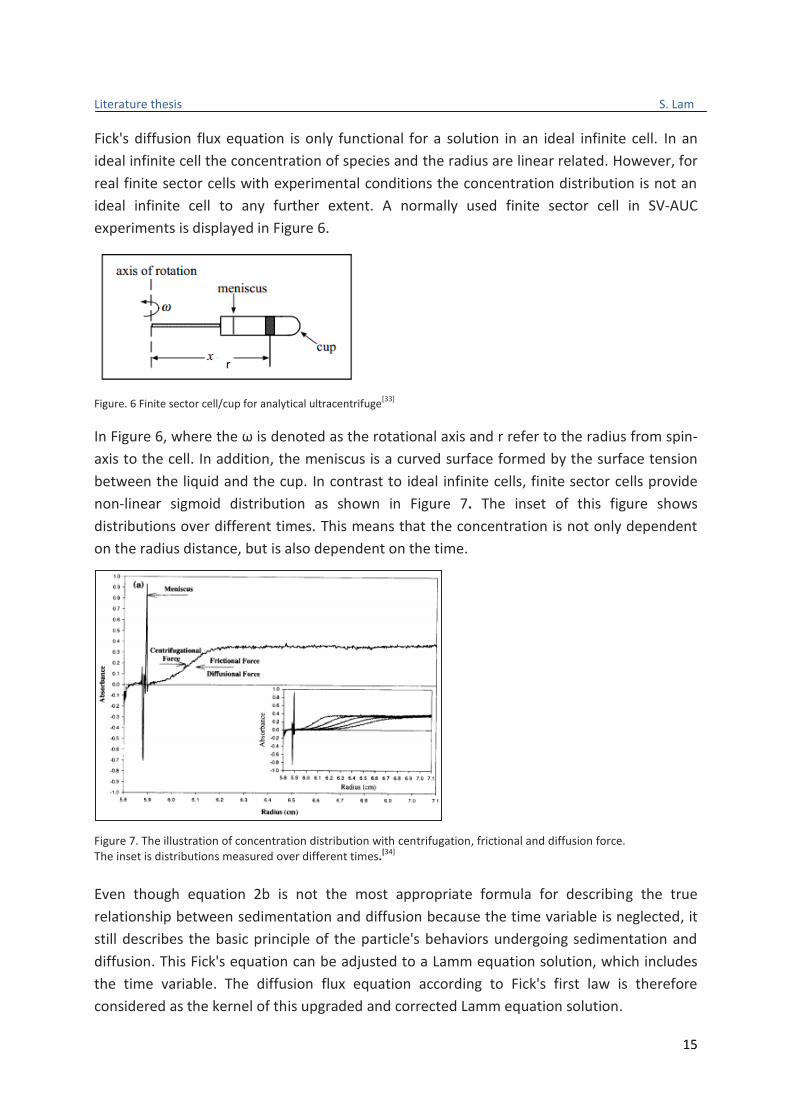
Fick's diffusion flux equation is only functional for a solution in an ideal infinite cell. In an
ideal infinite cell the concentration of species and the radius are linear related. However, for
real finite sector cells with experimental conditions the concentration distribution is not an
ideal infinite cell to any further extent. A normally used finite sector cell in SV-AUC
experiments is displayed in Figure 6.
Figure. 6 Finite sector cell/cup for analytical ultracentrifuge
[33]
In Figure 6, where the ω is denoted as the rotational axis and r refer to the radius from spin-
axis to the cell. In addition, the meniscus is a curved surface formed by the surface tension
between the liquid and the cup. In contrast to ideal infinite cells, finite sector cells provide
non-linear sigmoid distribution as shown in Figure 7. The inset of this figure shows
distributions over different times. This means that the concentration is not only dependent
on the radius distance, but is also dependent on the time.
Figure 7. The illustration of concentration distribution with centrifugation, frictional and diffusion force. The inset is distributions measured over different times.[34]
Even though equation 2b is not the most appropriate formula for describing the true
relationship between sedimentation and diffusion because the time variable is neglected, it
still describes the basic principle of the particle's behaviors undergoing sedimentation and
diffusion. This Fick's equation can be adjusted to a Lamm equation solution, which includes
the time variable. The diffusion flux equation according to Fick's first law is therefore
considered as the kernel of this upgraded and corrected Lamm equation solution.
r
Literature thesis S. Lam
16
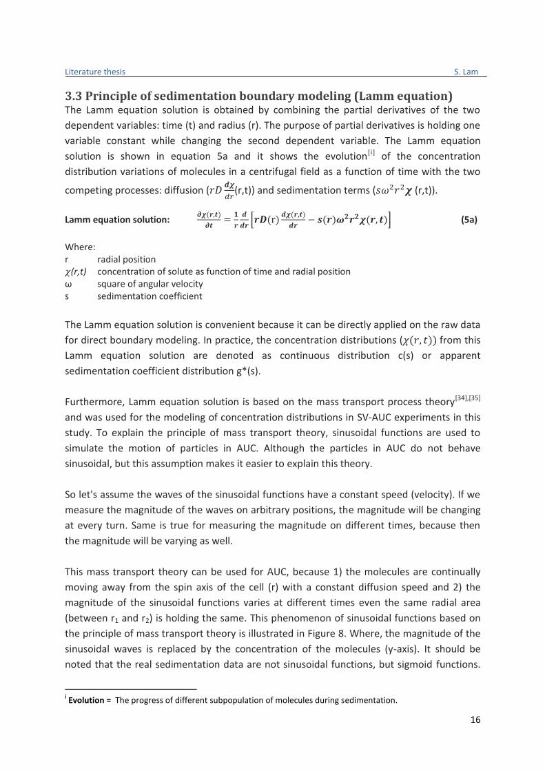
3.3 Principle of sedimentation boundary modeling (Lamm equation) The Lamm equation solution is obtained by combining the partial derivatives of the two
dependent variables: time (t) and radius (r). The purpose of partial derivatives is holding one
variable constant while changing the second dependent variable. The Lamm equation
solution is shown in equation 5a and it shows the evolution[i] of the concentration
distribution variations of molecules in a centrifugal field as a function of time with the two
competing processes: diffusion (
(r,t)) and sedimentation terms ( (r,t)).
Lamm equation solution:
(5a)
Where: r radial position (r,t) concentration of solute as function of time and radial position ω square of angular velocity s sedimentation coefficient
The Lamm equation solution is convenient because it can be directly applied on the raw data
for direct boundary modeling. In practice, the concentration distributions ( from this
Lamm equation solution are denoted as continuous distribution c(s) or apparent
sedimentation coefficient distribution g*(s).
Furthermore, Lamm equation solution is based on the mass transport process theory[34],[35]
and was used for the modeling of concentration distributions in SV-AUC experiments in this
study. To explain the principle of mass transport theory, sinusoidal functions are used to
simulate the motion of particles in AUC. Although the particles in AUC do not behave
sinusoidal, but this assumption makes it easier to explain this theory.
So let's assume the waves of the sinusoidal functions have a constant speed (velocity). If we
measure the magnitude of the waves on arbitrary positions, the magnitude will be changing
at every turn. Same is true for measuring the magnitude on different times, because then
the magnitude will be varying as well.
This mass transport theory can be used for AUC, because 1) the molecules are continually
moving away from the spin axis of the cell (r) with a constant diffusion speed and 2) the
magnitude of the sinusoidal functions varies at different times even the same radial area
(between r1 and r2) is holding the same. This phenomenon of sinusoidal functions based on
the principle of mass transport theory is illustrated in Figure 8. Where, the magnitude of the
sinusoidal waves is replaced by the concentration of the molecules (y-axis). It should be
noted that the real sedimentation data are not sinusoidal functions, but sigmoid functions.
i Evolution = The progress of different subpopulation of molecules during sedimentation.
Literature thesis S. Lam
17
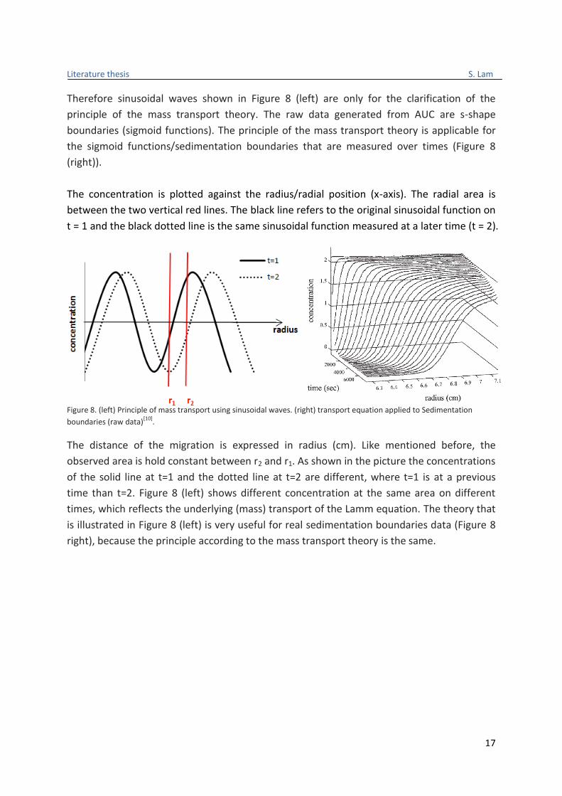
Therefore sinusoidal waves shown in Figure 8 (left) are only for the clarification of the
principle of the mass transport theory. The raw data generated from AUC are s-shape
boundaries (sigmoid functions). The principle of the mass transport theory is applicable for
the sigmoid functions/sedimentation boundaries that are measured over times (Figure 8
(right)).
The concentration is plotted against the radius/radial position (x-axis). The radial area is
between the two vertical red lines. The black line refers to the original sinusoidal function on
t = 1 and the black dotted line is the same sinusoidal function measured at a later time (t = 2).
Figure 8. (left) Principle of mass transport using sinusoidal waves. (right) transport equation applied to Sedimentation
boundaries (raw data)[10]
.
The distance of the migration is expressed in radius (cm). Like mentioned before, the
observed area is hold constant between r2 and r1. As shown in the picture the concentrations
of the solid line at t=1 and the dotted line at t=2 are different, where t=1 is at a previous
time than t=2. Figure 8 (left) shows different concentration at the same area on different
times, which reflects the underlying (mass) transport of the Lamm equation. The theory that
is illustrated in Figure 8 (left) is very useful for real sedimentation boundaries data (Figure 8
right), because the principle according to the mass transport theory is the same.
Literature thesis S. Lam
18
3.4 Sedimentation coefficient The motion of the sedimentation boundary as a function of time is typically used to
determine the sedimentation coefficient (s)[36],[37], diffusion coefficient (-D) and homogeneity.
Diffusion coefficient was already explained in the previous section, but the sedimentation
coefficient is a new introduced parameter derived from the Lamm equation solution. This
parameter is important because it characterizes the protein's or protein aggregate's
behaviors undergoing the sedimentation process using boundary sedimentation velocity.
The equation of sedimentation coefficient according to Svedberg theory is given as follow:
Sedimentation coefficient :
(6a)
Where: a centrifugal acceleration u velocity ω square of angular velocity or angular momentum
Sedimentation coefficient is expressed in Svedberg unit (S)[17],[38] or 10-13sec and is the
velocity of the particle per unit gravitational acceleration. To keep it simple and not going
into details of physics is actually an intuition of centrifugal acceleration from AUC. It is
important to know that the velocity of a molecule in a centrifugal field depends on the
physical properties of the molecule. Molecules with different properties will have a different
velocity in a centrifugal field. Sedimentation coefficient does not solely depend on the
acceleration but more on the properties of the particles and the medium that the particles
are suspended in. The physical properties that the sedimentation coefficient is associated
with are: molecular weights (only significant for single molecules), shapes, sizes and
densities.
3.5 Apparent sedimentation coefficient Sedimentation coefficients (s) can also be determined for each individual radial point instead
of a specific boundary area (between r1 and r2). This is called an apparent sedimentation
coefficient (s*)[17],[39] and is dependent on the position, time and rotor speed. This parameter
is determined by the differential apparent sedimentation coefficient distribution g*(s)
method. This method will be discussed in chapter 5.1.
For the calculation of the apparent sedimentation coefficient, the boundary has to be
equally divided into boundary parts. Subsequently, the boundary parts will be cumulative
ranked in an ascending order. For cumulative ranking the maximum is set on 1 (or 100%
percentile) and the minimum is set on 0. Accordingly, the cumulative distribution ranges
from 0 to 1 or (0% - 100%). The plateau concentration is the maximum concentration that
has reached the saturation absorbance level. The corresponding radius of this maximum is
the plateau radius (rp). The minimum of this distribution is the radius at meniscus (rm).The
calculation of the apparent sedimentation coefficient is shown in equation 6b.

Literature thesis S. Lam
19
Apparent sedimentation coefficient
(6b)
Where: ω square of angular velocity or angular momentum t time ri/rp boundary fraction rp radius at plateau ri radius that is taking from the cumulative distribution
As shown in equation 6b, a boundary fraction is calculated by ri/rp (i = 0.1, 0.2,...,1). The
illustration of this theory for estimating the apparent sedimentation coefficient g*(s) is
shown in Figure 9.
Figure 9. Cumulative distribution of sedimentation boundary to determine the apparent sedimentation coefficient (s*). This
graph with boundary fraction as the y-axis is plotted against radius (x-axis)40
.
A shown in Figure 9, the boundary fraction can be selected by choosing any individual radius
point ( ) and divide it by rp to calculate the apparent sedimentation coefficient s*. For
example, if the selected radius is at the plateau concentration (rp), the calculated boundary
fraction is then rp/rp (r11/r11) which results 1 as shown in Figure 9. If the selected
concentration is at the meniscus (rm/rp, r1/r11) it is 0. The mobility of a particle at a specific
time corresponds to a sedimentation coefficient. Since the relation can be written as: ln(ri/rp)
= s*ωt, this relation can be better illustrated with Figure 10. The apparent sedimentation
coefficient s* is the slope of the sedimentation boundaries that are measured over time.
Figure 10. The illustration of calculating the apparent
sedimentation coefficient s*.[36]
slope = s*
Literature thesis S. Lam
20
4. Instrumentation
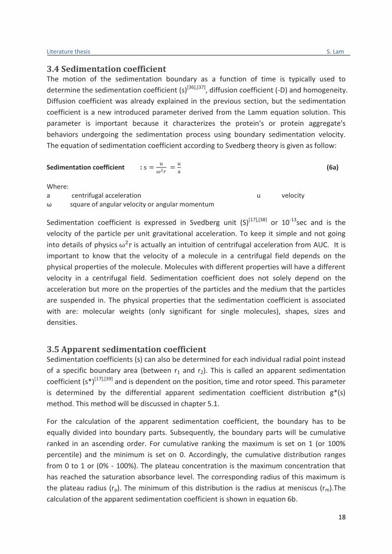
4.1 Analytical ultracentrifuge The AUC[41] is able to rotate at speeds up to 60,000 rpm, which creates a centrifugation force
of up to 250,000 g. This strong g-force is required to sediment small particles (i.e. proteins,
protein aggregates and contaminants). There are two types of analytical ultracentrifugation
that is introduced by Beckman Coulters Optima Instruments, the XLA and XLI. The difference
between the two AUC are the optics. XLA has UV and visible absorption optics and XLI has
integrated absorbance and interference optics. The detection optics XLA or XLI are normally
installed at the same AUC centrifuge. Accordingly, the selection in mode has to be initially
selected for XLA or XLI. The AUC from Optima with XL-A and XL-I optics is shown in Figure 11.
Figure 11. The Optima™ XL-A and the Optima XL-I analytical ultracentrifuges
[42].
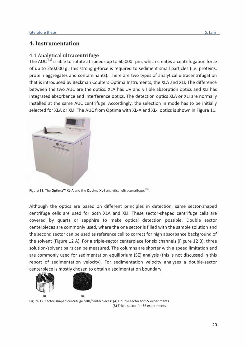
Although the optics are based on different principles in detection, same sector-shaped
centrifuge cells are used for both XLA and XLI. These sector-shaped centrifuge cells are
covered by quartz or sapphire to make optical detection possible. Double sector
centerpieces are commonly used, where the one sector is filled with the sample solution and
the second sector can be used as reference cell to correct for high absorbance background of
the solvent (Figure 12 A). For a triple-sector centerpiece for six channels (Figure 12 B), three
solution/solvent pairs can be measured. The columns are shorter with a speed limitation and
are commonly used for sedimentation equilibrium (SE) analysis (this is not discussed in this
report of sedimentation velocity). For sedimentation velocity analyses a double-sector
centerpiece is mostly chosen to obtain a sedimentation boundary.
Figure 12. sector-shaped centrifuge cells/centerpieces: (A) Double sector for SV experiments (B) Triple sector for SE experiments
Literature thesis S. Lam
21
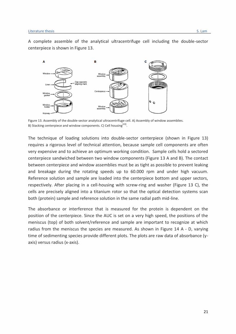
A complete assemble of the analytical ultracentrifuge cell including the double-sector
centerpiece is shown in Figure 13.
Figure 13. Assembly of the double-sector analytical ultracentrifuge cell. A) Assembly of window assemblies.
B) Stacking centerpiece and window components. C) Cell housing[43]
.
The technique of loading solutions into double-sector centerpiece (shown in Figure 13)
requires a rigorous level of technical attention, because sample cell components are often
very expensive and to achieve an optimum working condition. Sample cells hold a sectored
centerpiece sandwiched between two window components (Figure 13 A and B). The contact
between centerpiece and window assemblies must be as tight as possible to prevent leaking
and breakage during the rotating speeds up to 60.000 rpm and under high vacuum.
Reference solution and sample are loaded into the centerpiece bottom and upper sectors,
respectively. After placing in a cell-housing with screw-ring and washer (Figure 13 C), the
cells are precisely aligned into a titanium rotor so that the optical detection systems scan
both (protein) sample and reference solution in the same radial path mid-line.
The absorbance or interference that is measured for the protein is dependent on the
position of the centerpiece. Since the AUC is set on a very high speed, the positions of the
meniscus (top) of both solvent/reference and sample are important to recognize at which
radius from the meniscus the species are measured. As shown in Figure 14 A - D, varying
time of sedimenting species provide different plots. The plots are raw data of absorbance (y-
axis) versus radius (x-axis).

Literature thesis S. Lam
22
Figure 14. (A-D) Sedimentation plots of different times of sedimenting species.[46]
XLA[44] has UV and visible absorption optics and XLI[45] has integrated absorbance and
(Schlieren or Rayleigh) interference optics (Figure 15). Schlieren optics[34] measures the
refractive index gradient and is normally used for molecules that do not have (sufficient)
chromophores to use photoelectric absorbance. The refractive index gradient is directly
proportional to the concentration gradient; therefore the Schlieren readout can be used to
determine the concentration of protein solutions. Rayleigh interference optic is more
sensitive than Schlieren optic, so for modern AUC the Rayleigh optics are used. Rayleigh
optic has a higher refractive index, due to their light source (i.e. monochromatic light, laser).
A major advantage of refractive index optics is that they are not interfered by high
absorbance background of the solvent.
Figure 15. Comparison of the data obtained from the (a) schlieren, (b) XLI interference, (c) XLA absorbance optical
systems[34]
Literature thesis S. Lam
23
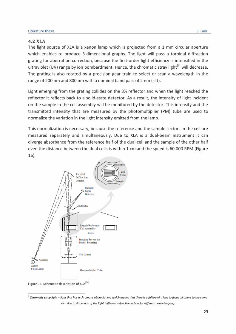
4.2 XLA The light source of XLA is a xenon lamp which is projected from a 1 mm circular aperture
which enables to produce 3-dimensional graphs. The light will pass a toroidal diffraction
grating for aberration correction, because the first-order light efficiency is intensified in the
ultraviolet (UV) range by ion bombardment. Hence, the chromatic stray light[ii] will decrease.
The grating is also rotated by a precision gear train to select or scan a wavelength in the
range of 200 nm and 800 nm with a nominal band pass of 2 nm (slit).
Light emerging from the grating collides on the 8% reflector and when the light reached the
reflector it reflects back to a solid-state detector. As a result, the intensity of light incident
on the sample in the cell assembly will be monitored by the detector. This intensity and the
transmitted intensity that are measured by the photomultiplier (PM) tube are used to
normalize the variation in the light intensity emitted from the lamp.
This normalization is necessary, because the reference and the sample sectors in the cell are
measured separately and simultaneously. Due to XLA is a dual-beam instrument it can
diverge absorbance from the reference half of the dual cell and the sample of the other half
even the distance between the dual cells is within 1 cm and the speed is 60.000 RPM (Figure
16).
Figure 16. Schematic description of XLA[34]
ii Chromatic stray light = light that has a chromatic abbreviation, which means that there is a failure of a lens to focus all colors to the same
point due to dispersion of the light (different refractive indices for different wavelengths).
Literature thesis S. Lam
24
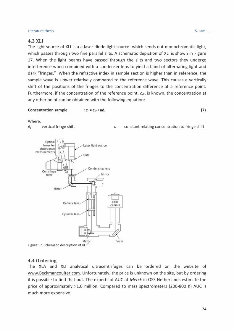
4.3 XLI The light source of XLI is a a laser diode light source which sends out monochromatic light,
which passes through two fine parallel slits. A schematic depiction of XLI is shown in Figure
17. When the light beams have passed through the slits and two sectors they undergo
interference when combined with a condenser lens to yield a band of alternating light and
dark “fringes.” When the refractive index in sample section is higher than in reference, the
sample wave is slower relatively compared to the reference wave. This causes a vertically
shift of the positions of the fringes to the concentration difference at a reference point.
Furthermore, if the concentration of the reference point, crF, is known, the concentration at
any other point can be obtained with the following equation:
Concentration sample : cr = crF +aΔj (7)
Where: Δj vertical fringe shift a constant relating concentration to fringe shift
Figure 17. Schematic description of XLI[34]
4.4 Ordering The XLA and XLI analytical ultracentrifuges can be ordered on the website of
www.Beckmancoulter.com. Unfortunately, the price is unknown on the site, but by ordering
it is possible to find that out. The experts of AUC at Merck in OSS Netherlands estimate the
price of approximately >1.0 million. Compared to mass spectrometers (200-800 K) AUC is
much more expensive.
Literature thesis S. Lam
25
4.5 Application of the AUC A frequently used experiment for analytical ultracentrifuge (AUC) is the sedimentation
velocity (SV) experiment. This method is carried out at very high speeds (40.000 - 60.000
rpm) and the measurement takes 1 - 3 hours, depending on what kind of experiment is in
progress. The high centrifugal force rapidly causes the migration of the proteins towards the
bottom of the sector and forms a sedimentation boundary. The concentration distribution
across the cell at various times and radius during the experiment is measured while the
sample is rotating. It measures the sedimentation rate at which the molecules migrate in
response to the centrifugation force in AUC. This sedimentation rate provides information
about:
sedimentation coefficient s-value
boundary shape of the proteins
Isotherm of the weight-average s-value
differential distribution coefficient of the molecules
Sedimentation velocity is particularly valuable for:
Detection of aggregate(s) in protein samples and also quantify the concentration of
the aggregate(s)
Verify the homogeneity of a sample
Establish the native state of a protein, monomer, dimers and so on.
Measure the size distribution in samples, small/large molecules only or mixture of
small and large molecules.
Study the formation of complexes between proteins (antigen-antibody complex or
receptor-ligand complex)

Literature thesis S. Lam
26
5. Analyses and approach
5.1 Apparent sedimentation coefficient distribution g*(s) analysis The apparent sedimentation coefficients can be estimated from sedimentation boundaries.
This can also be done for sedimentation boundaries over different measured times. The
envision of the DCDT+ approach is shown in Figure 18.
Figure 18. An envision of the chronological steps (1-4) to obtain g(s*) distribution that is derived by time derivative dcdt method.
[36]
Consequently, a collection of many s* is obtained and resulted s* distributions (step 2). By
performing the Lamm equation solution on the s* distributions, the normalized dc/dt
distribution was calculated (step 3). After simulating the dc/dt distribution, the apparent
sedimentation coefficient distributions g*(s) were obtained (step 4). Similar to a
chromatogram, the area under each peak gives the total concentration of species.
Apparent sedimentation coefficient distribution g(s*) considers the migration of boundary
and reflects the boundary shape. Even though this analysis is based on the Lamm equation
solution, this equation has to be adjusted. This is because the Lamm equation assumes
dealing with diffusing species, whereas g*(s) is assuming to have non-diffusing species. The
adjusted and converted equation derives the modeling of g*(s) distributions (shown in
Figure 19).
Lamm-equation Differential distribution of non-diffusing species
Figure 19. The conversion of a differential distribution of non-diffusing species for modeling g*(s) from Lamm-equation
modeling.
Conversion

Literature thesis S. Lam
27
Where, r is radius; t is time; s is sedimentation coefficient; D is diffusion coefficient; and is
residual. Figure 18 shows the direct boundary model where the solution of single species of
the Lamm-equation is replaced by the theoretical sedimentation profiles of
non-diffusing species . The measured sedimentation profile, absorbance or
interference profiles are given as c(r,t). The measured profiles are modeled as an integral
over the differential concentration distribution c(s) for Lamm equation and sedimentation
coefficient distribution g*(s) for the converted equation. The converted apparent
distribution is assumed to have no diffusion (D (s) = 0).
A major drawback of g*(s) analysis is the low resolution and sensitivity of the sedimentation
coefficient distributions for mixtures of species with different sizes; This is typically caused
by neglecting the diffusion process. To solve this drawback, a differential sedimentation
coefficient analysis was taken into account for this study. In contrast to g*(s), this c(s)
analysis includes diffusion. In this paper, these two analyses will be compared with each
other for the determination of protein aggregates and contaminants. The principle of the c(s)
analysis will be explained in the following paragraph.
5.2 Sedimentation coefficient distribution c(s) analysis The c(s) distribution is used to calculate a sedimentation distribution of species taking into
account their diffusion and is based on the Lamm equation solution (equation 5a). This
method is computationally the most complex approach, yet it has the potential for
improving resolution and sensitivity in respect to g*(s). For simple and fast measurements,
g*(s) is still the recommended analysis for modeling the data.
Because the use of numerical solutions of the Lamm equation, it has no constraints in the
data set that can be considered for analysis. Additionally, this is the most general
sedimentation approach with respect to size range for the distribution. However, there are
some key assumptions made in this technique in the form of statistical and experimental
prior knowledge, which must be properly adjusted to avoid wrong interpretation of results:
(1) The strategy uses hydrodynamic prior knowledge (weight-average frictional ratio) to
estimate the extent of diffusion for each species and 2) validation of prior assumptions is
necessary.
An example of the differential sedimentation distribution c(s) that is plotted against the
sedimentation coefficient which was determined by the mathematical data analysis program
SEDFIT is shown in Figure 18 B. Because this program makes use of the Lamm equation
solution, the distribution of sedimentation coefficient vs. c(s) (Figure 20 B) links with the
direct sedimentation boundaries modeling results (Figure 20 A). This modeling is done by
statistical criteria involving the (non-linear) least squares method.

Literature thesis S. Lam
28
Figure 20 A. direct sedimentation boundaries modelling
[9] Figure 20 B. c(s) versus sedimentation coefficient (s) [9]
Figure 20 B shows profiles similar to a chromatograms and the relative (loading)
concentration can be assessed by the area under the curve with different s-values. The c(s)
analysis is a frequently selected analysis for the determination of protein aggregates in
therapeutic drugs. In this paper, this analysis will be partly compared to the g*(s) analysis,
which provides apparent sedimentation coefficient distributions. The g*(s) analysis also
provides profiles that are similar to chromatograms, yet this analysis differ from c(s) analysis
because g*(s) analysis is based on a different principle.
5.3 Therapeutic product related impurities (contaminations) Proteins are macromolecules that are composed of amino acids. In this report it will mainly
discuss about protein aggregates and contaminating species. The contaminants are normally
present in the protein mixtures in small size and amount. Small species have sizes below
50kD and large proteins (aggregates) have sizes above 50kD. Generally, the SV-AUC method
can achieve several distributions (in this study, i.e.: c(s) and g(s*)) to characterize different
protein mixtures. The characterization of these protein mixture in this literature thesis
focuses on reactions containing contaminations, with emphasis on specific factors such as: 1)
homogeneity of the product and 2) detecting small soluble oligomers (e.g. dimers, trimers,
etc.), while comparing c(s) and g(s*) analyses.
5.4 Approach and interpretation of the applications Heterogeneous interactions are defined as interactions in which two (or more) reactants (A
and/or B) from mixtures containing two species (like protein A and B), reversibly form a
complex with a specific stoichiometry. Examples of such interactions would follow
association schemes like A + B ⇔ AB; A + 2B ⇔ AB 2 ; AB + B ⇔ AB 2 ; etc. Self-association
reversible system or multiple reactions are slightly different than heterogeneous interactions
and can be written as: (A + A + B ⇔ A2), where the concentration from one component
affects the concentration of the other component.

Literature thesis S. Lam
29
The homogeneity of (protein) products can be determined by SV-AUC. The c(s) distribution
from a certain protein product, shown in Figure 21 will be expected.
Figure 21. Full c(s) distributions of the protein that contains 4.7 % dimer, 1.8% trimer, 1.1% tetramer and 0.7% low mass contaminant, where the percentage is based on the total protein. Inset: Enlarged c(s) distributions to show the low mass contaminant at 2S
[46].
Figure 21 shows a heterogeneous system, because we observe the amount of species
sedimenting at different rates, which are expressed in sedimentation coefficients (S).
In contrast to normal reversible systems, self-association proteins are more complex. This
system occurs when the protein has an intramolecular binding with itself and this dimer,
trimer, tetramer, etc. (Figure 22). Figure 22. Ultracentrifugation c(s) distribution analyses of full-length Factor H and three fragments. (A-C) The monomer is denoted by 1, the dimer by 2, and so on, where the c(s) is the y-axis and sedimentation coefficient is the x-axis. It can be noticed that SCR-1/5 forms only monomer (a), SCR-6/8 forms monomer and a small amount of dimer (b), and SCR-16/20 forms almost equal amounts of monomer and dimer (c). (D) shows the full-length Factor H, boundary scans measured at 5.92 mg/mL and 0.17 mg/mL are shown in red and the boundary fits are shown in black. (F) The five c(s) analyses for Factor H between 0.17 mg/mL (bottom) and 5.92 mg/mL (top) revealed the monomer and a series of oligomers labeled from 2 to 7.
[47]
Literature thesis S. Lam
30
This type of system makes it looks like the monomer has a higher concentration and is
typically an occurrence of self-associating systems. Because when macromolecules associate
with itself, the molecular weight increases. Consequently, the sedimentation coefficient will
increase with increasing concentration.
In Figure 22 D the perturbations show the existence of more rapidly sedimenting species.
Figure 22 F shows that above a certain concentration of Factor H (about 10 % - 15 %), Factor
H will be dimeric if no other factors influence the equilibrium and this results the appearance
of peak number 2 at every measurement that is shown in Figure 22 F, while other oligomers
(numbers 3 - 7 ) vanish at some measurement series and present in other series.
Literature thesis S. Lam
31
6. Applications
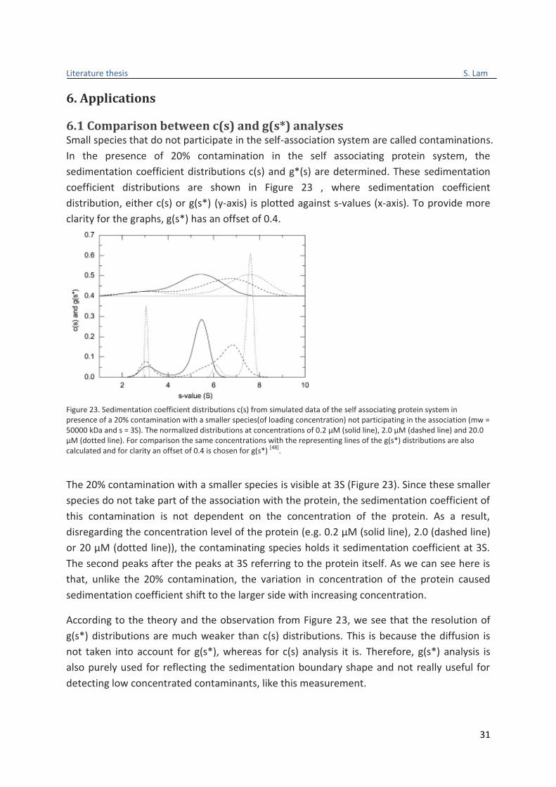
6.1 Comparison between c(s) and g(s*) analyses Small species that do not participate in the self-association system are called contaminations.
In the presence of 20% contamination in the self associating protein system, the
sedimentation coefficient distributions c(s) and g*(s) are determined. These sedimentation
coefficient distributions are shown in Figure 23 , where sedimentation coefficient
distribution, either c(s) or g(s*) (y-axis) is plotted against s-values (x-axis). To provide more
clarity for the graphs, g(s*) has an offset of 0.4.
Figure 23. Sedimentation coefficient distributions c(s) from simulated data of the self associating protein system in presence of a 20% contamination with a smaller species(of loading concentration) not participating in the association (mw = 50000 kDa and s = 3S). The normalized distributions at concentrations of 0.2 µM (solid line), 2.0 µM (dashed line) and 20.0 µM (dotted line). For comparison the same concentrations with the representing lines of the g(s*) distributions are also calculated and for clarity an offset of 0.4 is chosen for g(s*)
[48].
The 20% contamination with a smaller species is visible at 3S (Figure 23). Since these smaller
species do not take part of the association with the protein, the sedimentation coefficient of
this contamination is not dependent on the concentration of the protein. As a result,
disregarding the concentration level of the protein (e.g. 0.2 µM (solid line), 2.0 (dashed line)
or 20 µM (dotted line)), the contaminating species holds it sedimentation coefficient at 3S.
The second peaks after the peaks at 3S referring to the protein itself. As we can see here is
that, unlike the 20% contamination, the variation in concentration of the protein caused
sedimentation coefficient shift to the larger side with increasing concentration.
According to the theory and the observation from Figure 23, we see that the resolution of
g(s*) distributions are much weaker than c(s) distributions. This is because the diffusion is
not taken into account for g(s*), whereas for c(s) analysis it is. Therefore, g(s*) analysis is
also purely used for reflecting the sedimentation boundary shape and not really useful for
detecting low concentrated contaminants, like this measurement.
Literature thesis S. Lam
32
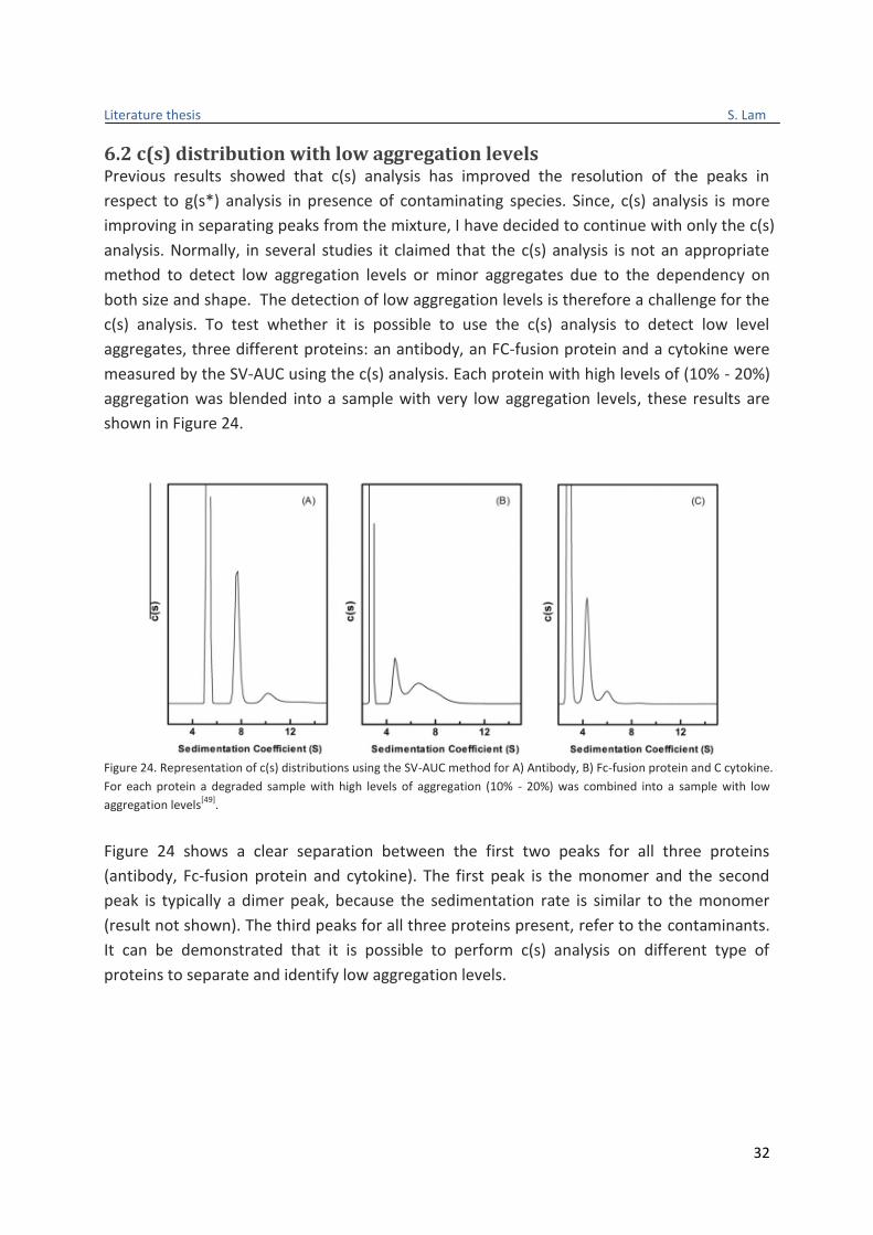
6.2 c(s) distribution with low aggregation levels Previous results showed that c(s) analysis has improved the resolution of the peaks in
respect to g(s*) analysis in presence of contaminating species. Since, c(s) analysis is more
improving in separating peaks from the mixture, I have decided to continue with only the c(s)
analysis. Normally, in several studies it claimed that the c(s) analysis is not an appropriate
method to detect low aggregation levels or minor aggregates due to the dependency on
both size and shape. The detection of low aggregation levels is therefore a challenge for the
c(s) analysis. To test whether it is possible to use the c(s) analysis to detect low level
aggregates, three different proteins: an antibody, an FC-fusion protein and a cytokine were
measured by the SV-AUC using the c(s) analysis. Each protein with high levels of (10% - 20%)
aggregation was blended into a sample with very low aggregation levels, these results are
shown in Figure 24.
Figure 24. Representation of c(s) distributions using the SV-AUC method for A) Antibody, B) Fc-fusion protein and C cytokine.
For each protein a degraded sample with high levels of aggregation (10% - 20%) was combined into a sample with low
aggregation levels[49]
.
Figure 24 shows a clear separation between the first two peaks for all three proteins
(antibody, Fc-fusion protein and cytokine). The first peak is the monomer and the second
peak is typically a dimer peak, because the sedimentation rate is similar to the monomer
(result not shown). The third peaks for all three proteins present, refer to the contaminants.
It can be demonstrated that it is possible to perform c(s) analysis on different type of
proteins to separate and identify low aggregation levels.

Literature thesis S. Lam
33
6.3 Therapeutic monoclonal antibodies homogeneity Protein aggregation is a major problem for therapeutic proteins like monoclonal antibodies
(MAb), because it can affect the stability of these products. Therefore the homogeneity of
these proteins were tested by using SV-AUC (c(s) analysis). Two types of MAb: MAb-a and
MAb-b were measured at standard conditions of 20C and after heating. Heating is one of the
methods to deliver stress to the antibodies. The results for antibody MAb-a and MAb-B are
shown in Figure 25 and Figure 26, respectively.
Figure 25. Left: SV-AUC analysis of approximately 0.5 mg/ml monoclonal antibody MAb-a, at 50.000 rpm, and 20C in 50 mM Tris-HCl, 0.1 M NaCl, pH 7.5. Right: SV-AUC analysis of the same antibody from the left after heating. A) Raw sedimentation boundaries and B) sedimentation coefficient distributions c(s) derived from A)
[5].
As shown in Figure 25, the higher the molecular weight of antibodies means that the moving
boundaries for antibodies are less broadened by diffusion and the separation is more
improving. This is an important reason why it is necessary to mathematically resolve so
many components and detect peaks present at levels of only a few tenths of a percent (low
levels aggregates).
This MAb-A antibody starts off with a higher aggregate content of 5.7% (sum of aggregates %
at 9.57 S, 12.1 S and 16.0 S). After heating, the MAb-a sample becomes quite heterogeneous
(materials are sedimenting at different sedimentation coefficients).

Literature thesis S. Lam
34
Figure 26. Left: SV-AUC analysis of approximately 0.5 mg/ml monoclonal antibody MAb-b, at 50.000 rpm, and 20C in 50 mM Tris-HCl, 0.1 M NaCl, pH 7.5. Right: SV-AUC analysis of the same antibody from the left after heating. A) Raw sedimentation boundaries and B) sedimentation coefficient distributions c(s) derived from A)
[5].
Figure 26 on the left shows that the monomer of antibody MAb-b has a sedimentation
coefficient of 6.63 S and accounts for 95.7% of the total sedimenting solutes. The species at
9.13 S and at 11.6 S, which accounts for 3.1% and 1.1% off the total, are probably a dimer
and trimer (results not shown). In this experiment the parameters such as shape, size and
sedimentation rate were unfortunately not taken into account, therefore the dimer and
trimer can only be empirically assumed that they present.
After the sample was subjected to heat stress (Figure 26 right), it shows a decrease to only
56.2 % of the monomer. Additionally, at least eight peaks of aggregates are detected. The
most prominent aggregate peaks at 9.90, 12.7, 15.1, 17.3, and 20.2 S fall very close to the
positions expected (relative to monomer) for dimer, trimer, tetramer, pentamer, and
hexamer based on model hydrodynamic calculations (results not shown).
Interestingly the distributions of aggregates formed by the two antibodies MAb-a and MAb-b
are different even though heat stress produced about 50% total aggregate for both.
Additionally the results of both antibodies showed that after heating they both are having a
heterogeneous system.

Literature thesis S. Lam
35
6.4 Fluorescence detection The more recent additional detection with fluorescence extends the flexibility of analytical
ultracentrifugation with respect to the existing absorbance and interference detectors
dramatically. It is claimed that fluorescence detection gives a strong improvement of the
applicability of AUC compared to the two former detection modes[59].
Earlier in this report absorbance and interference detections are discussed, because these
detections are commonly used. Fluorescence detection complements these two detections,
because it allows AUC analysis for strongly diluted solutions. An example of the titration of
Alexa-488 labeled, goat anti-mouse lgG into a fixed concentration of mouse lgG in 100 mM
KCl 20 mM Tris pH 8, 0.1 mg/ml ovalbumin is shown in Figure 27. The sedimentation
coefficient distributions c(s) of the presence (dotted lines) and absence (solid line) of a fixed
concentration mouse lgG to different concentrations of Alexa-488 labeled lgG.
Figure 27. Titration of Alexa-488 labeled goat anti-mouse lgG into a fixed concentration of mouse lgG in 100 mM KCl 20 mM
Tris pH 8, 0.1 mg/ml ovalbumin. For each concentration of Alexa-488 labeled lgG in presence (dotted line) or absence (solid
line) of a fixed concentration mouse lgG, a c(s) distribution has been determined. The data have been normalized on every
c(s) distribution[48]
.
The labeled Alexa-488 lgG without mouse lgG (dotted lines) are fixed on the peak position of
6.8 S, which is consistent of being a monomer. The complex formations of labeled Alexa-488
lgG and mouse lgG (solid lines) shift to higher s-values. Interestingly, when labeled Alexa-488
lgG is in a high concentration with mouse lgG (red line, 70 nM), the peak of the complex
formation has shifted (back) to a lower s-value. This indicates that the antibody is in excess
in the solution. The shifts in s-values indicate that low-concentration sample compounds in
complex mixtures can be determined due to the high sensitivity and selectivity of
fluorescence detection.

Literature thesis S. Lam
36
7. Conclusion
Protein aggregation is often a major problem for therapeutic proteins. Contaminants (such
as: non-protein, host cell protein materials or damaged form of the protein product itself)
often lead to accumulation of protein aggregates. The formation of protein aggregates can
cause serious damage to the therapeutic product; therefore experiments are carried out to
determine the homogeneity of the product and to detect small soluble oligomers. The
experiments were performed by the sedimentation velocity ultracentrifugation (SV-AUC).
The selected sedimentation distribution analyses for modeling the raw sedimentation
moving boundaries data are: c(s) and g(s*). These two analyses were supported by the data
analysis programs: SEDFITfor c(s) and DCDT+ for g(s*). The former analysis includes diffusion,
whereas the latter analysis does not. By comparing c(s) and g(s*) analyses (Applications from
6.1) I observed that the resolution and sensitivity of c(s) is more improving due to direct
fitting of sedimentation profiles with Lamm equation modeling, which includes diffusion
process. Thus after comparison I have decided to continue with solely the c(s) analysis for
the next experiments.
From the results obtained with SV-AUC and c(s) modeling I can conclude that:
1) It is possible to detect low levels aggregates (small soluble oligomers) in different type of
therapeutic proteins.
2) Homogeneity or heterogeneity of therapeutic antibodies can be properly characterized.
Overall, it can be concluded that the SV-AUC is a very useful technique in characterizing and
detecting protein aggregates in the size range of SV-AUC 1.0 nm - 110 nm (typically
measuring range for protein aggregates, monomers and oligomers) and compared to other
techniques this is a non-destructive method because it has a matrix- and column-free
approach.
8. Discussion
Fluorescence detection has a higher selectivity than absorbance and interference and is
therefore able to detect low concentration (highly diluted) species in complex protein
mixtures by observing the shifts in s-values.
Literature thesis S. Lam
37
References 1 Rosenberg AS. Effects of protein aggregates: an immunologic perspective. The AAPS journal 2006;8(3):501-07.
2 Arakawa T, Philo JS, Ejima D, Tsumoto K, Arisaka F. Aggregation analysis of therapeutic proteins, part 1.
Bioprocess International 2006;4(10):32-42. 3 Byeong S, Herhenson S. Practical approaches to protein formulation development. Practical approaches to
protein formulation development. in "Rationale Design of stable protein formulations-theory and practice" (J.F. Carpenter and M.C. Manning eds.) Kluwer Academic/Plenum publishers, New York, pp. 1-25 4 Arakawa T, Philo JS, Ejima D, Tsumoto K, Arisaka F. Aggregation analysis of therapeutic proteins, part 2
Analytical ultracentrifugation and dynamic light scattering. Bioprocess International 2007;4(10):36-47. 5 Guidance for Industry Immunogenicity Assessment for Therapeutic Protein Products, U.S. Department of
Health and Human Services Food and Drug Administration. Center for Drug Evaluation and Research (CDER). Center for Biologics Evaluation and Research (CBER) 2013 6 Schellekens H. Factors influencing the immunogenicity of therapeutic proteins.
Nephrology Dialysis Transplantation 2005;20(suppl 6):vi3-vi9. 7 Fang Y, Gao S, Tai D, Middaugh C R, Fang J. Identification of properties important to protein aggregation using
feature selection. BMC Bioinformatics 2013, 14:314 8 McPherson G. Beyond the speed of light (scattering), Bioprocess international april 2012
9 Krayukhina E, Uchiyama S, Nojima K, Okada Y, Hamaguchi I, Fukui K. Aggregation analysis of pharmaceutical
human immunoglobulin preparations using size-exclusion chromatography and analytical ultracentrifugation sedimentation velocity. Journal of Bioscience and Bioengineering Volume 115, Issue 1, January 2013, Pages 104–110 10
Lebowitz J, Lewis M.S, Schuck P. Modern analytical ultracentrifugation in protein science: A tutorial review. Protein sci. 2002 September, 11(9); 2067 - 2079. 11
Mittal V, Lechner M.D. Size and density dependent sedimentation analysis of advanced nanoparticle systems. Journal of Colloid and Interface Science Volume 346, Issue 2, 15 June 2010, Pages 378–383 12
Schuck P. On the analysis of protein self-association by sedimentation velocity analytical ultracentrifugation. Anal Biochem. 2003;320:104–124. 13
Laue TM. Sedimentation equilibrium as a thermodynamic tool. Methods Enzymol. 1995;259:427–452. 14
Van Holde K.E., Baldwin R. L., J. Phys. Chem. 62 (1958) 734 15
Howlett G.J, Minton A.P, Rivas G. Analytical ultracentrifugation for the study of protein association and assembly. Volume 10, Issue 5, October 2006, pages 430-436. 16
Zolls S, Tantipolphan R, Wiggenhorn M, Winter G, Jiskoot W, Friess W, Hawe A.Particles in therapeutic protein formulations, Part 1: Overview of analytical methods. Journal of pharmaceutical sciences, 2011
18
Dam J, Velikovsky C.A, Mariuzza R.A, Urbanke C, Schuck P. Sedimentation Velocity Analysis of Heterogeneous Protein-Protein Interactions: Lamm Equation Modeling and Sedimentation Coefficient Distributions c(s). Biophysical Journal Volume 89 July 2005 619–634
Literature thesis S. Lam
38
19
Zhao H, Balbo A, Brown P.H, Schuck P. The boundary structure in the analysis of reversibly interacting systems by sedimentation velocity, Methods 54 (2011) 16–30 20
Schuck P. Size-Distribution Analysis of Macromolecules by Sedimentation Velocity Ultracentrifugation and Lamm Equation Modeling. Biophysical Journal Volume 78 March 2000 1606–1619 21
Walter F, Stafford III. Boundary analysis in sedimentation transport experiments: A procedure for obtaining sedimentation coefficient distributions using the time derivative of the concentration profile. Analytical biochemistry 203, 295-301 (1992). 22
Stafford W. F., ‘Method for obtaining sedimentation coefficient distributions’ in Harding S. E., Rowe A. J.,Horton J. C., Analytical ultracentrifugation in biochemistry and polymer science. The royal society of chemistry, Cambridge (1992) 359.
23 Stafford W. F., Boundary analysis in sedimentation transport experiments: a procedure for obtaining
sedimentation coefficient distributions using the time derivative of the concentration profile. Anal Biochem.
1992, 203 (2); 295 - 301
24
Schuck P. Sedimentation Analysis of Noninteracting and Self-Associating Solutes Using Numerical Solutions to the Lamm Equation. Biophysical Journal Volume 75 September 1998 1503–1512 25
Schuck P. On the analysis of protein self-association by sedimentation velocity analytical ultracentrifugation. Analytical Biochemistry 320 (2003) 104–124 26
Schuck P. Diffusion-deconvoluted sedimentation coefficient distributions for the analysis of interacting and non-interacting protein mixtures. Chapter for “Modern Analytical Ultracentrifugation: Techniques and Methods ” (D.J. Scott, S.E.Harding, A.J. Rowe, Editors) The Royal Society of Chemistry, Cambridge (in press) 27
Balbo A, Minor K.H, Velikovsky C.A, Mariuzza R.A, Peterson C.B, Schuck P. Studying multiprotein complexes by multisignal sedimentation velocity analytical ultracentrifugation. University of California, Berkeley, CA, November 11, 2004 28
Ralston G; Introduction to Analytical Ultracentrifugation, Beckman Coulter Inc. Fullerton, US. 29
Lloyd P.H. Optical Methods In Ultracentrifugation, Electrophoresis, and Diffusion; Clarendon Press, Oxford 1974 30
Mücke N et al.: Molecular and Biophysical Characterization of Assembly-Starter Units of Human Vimentin. J Mol Biol. 2004 Jun 25;340(1):97-114. 31
Lecture: Introduction to material science for engineers chapter 5. University of Tennessee 32
Serdyuk I.N, Zaccai N.R, Zaccai J. Methods in Molecular Biophysics: Structure, Dynamics, Function. Cambridge University press. May 14, 2007. Edition 1. 33
Roberts R. lecture 6. http://www.its.caltech.edu/~ch24/lecture6.pdf 34
Moore J.D. Introduction to partial differential equations, May 21, 2003 35
Lenstra A. Lecture Math for HLO bachelor, 2013 36
http://www.analyticalultracentrifugation.com/sedfit_help_analytical_zone_centrifugation.htm
Literature thesis S. Lam
39
37
http://www.ap-lab.com/sedimentation_velocity.htm 38
Schuck P. Determination of the sedimentation coefficient distribution by least-squares boundary modeling. Biopolymers. 2000 Oct 15;54(5):328-41. 39
van Holde, K. E. and W. O. Weischet. Boundary Analysis of Sedimentation Velocity Experiments with Monodisperse and Paucidisperse Solutes. Biopolymers, 17 (1978); 1387-1403 40
Demeler, B. and K. E. van Holde. Sedimentation velocity analysis of highly heterogeneous systems. Anal. Biochem. 2004, Vol 335 (2); 279-288 42
https://www.beckmancoulter.com 43
Cole J.L, Hansen J.C. Analytical Ultracentrifugation as a Contemporary Biomolecular Research Tool. J Biomol Tech. 1999 December; 10(4): 163–176. 44
Demeler B, Saber H. Determination of Molecular Parameters by Fitting Sedimentation Data to Finite-Element Solutions of the Lamm Equation. Biophysical Journal Volume 74 January 1998; 444–454 45
MacGregor I.K, Anderson A.L, Laue T.M. Fluorescence detection for the XLI analytical ultracentrifuge. Biophysical Chemistry 108 (2004) 165–185 46
http://www.ap-lab.com/sedimentation_velocity.htm 47
Perkins S.J, Nan R, Li K, Khan S, Miller A. Complement Factor H–ligand interactions: Self-association, multivalency and dissociation constants. Immunobiology 217 (2012) 281–297 48
Laue T. Analytical ultracentrifugation: a powerful ‘new’ technology in drug discovery. Drug Discovery Today: Technologies, Vol 1, No.3, 2004; 309-315. 49
Gabrielson J.P Arthur K.K. Measuring low levels of protein aggregation by sedimentation velocity. Methods 54 (2011); 83–91