Embed Size (px)
Citation preview
This is a preprint of an article accepted for publication in Journal of Cold Regions
Science and Technology on 17 December 2012. The published article is available online at
http://www.sciencedirect.com/science/article/pii/S0165232X12002480
To be cited as: Goulmot D., Bouaanani N. 2013. Seismic analysis of rectangular water-containing structures
with floating ice blocks. Journal of Cold Regions Science andTechnology, 90-91: 22–32.
Seismic Analysis of Rectangular Water-ContainingStructures with Floating Ice Blocks
Damien Goulmot1 and Najib Bouaanani2
ABSTRACT
This paper presents a new formulation to investigate the effects of floating ice blocks on seismically-excited
rectangular water-containing structures. The proposed method is based on a sub-structuring approach, where the
flexible containing structure and ice-added mass are modeled using finite elements, while hydrodynamic effects
are modeled analytically through interaction forces at thewater-structure and water-ice interfaces, thus eliminat-
ing the need for reservoir finite element discretization. Inaddition to accounting for the influence of floating ice
blocks and container walls’ flexibility, the developed frequency- and time-domain techniques also include the ef-
fects of container geometrical or material asymmetry as well as the coupling between convective and impulsive
components of hydrodynamic pressure. The proposed formulation is illustrated through a numerical example il-
lustrating the dynamic response of symmetric and asymmetric water-containing structures covered with floating
ice blocks. Obtained time- and frequency-domain responsesare successfully validated against advanced finite
element analyses including fluid-structure interaction capabilities. For the water-containing structures studied,
the results show that the presence of floating ice blocks affects the frequency content and amplitudes of the
dynamic responses corresponding to convective and impulsive modes.
Key words: Dynamic response; Water-containing structure; Ice effects; Floating ice blocks; Sloshing ice;
Hydrodynamic pressure.
1 Graduate Research Assistant, Department of Civil, Geological and Mining Engineering,École Polytechnique de Montréal, Montréal, QC H3C 3A7, Canada.2 Professor, Department of Civil, Geological and Mining Engineering,École Polytechnique de Montréal, Montréal, QC H3C 3A7, CanadaCorresponding author. E-mail: [email protected]
1 Introduction
The dynamic behavior of water-containing structures has been widely studied in the last five decades
to predict their response to seismic excitations and prevent heavy damage as observed during the 1960
Chilean Earthquakes (Steinbrugge and Flores, 1963), the 1964 Alaska Earthquake (Hanson, 1973), and
more recently the 1994 Northridge Earthquake (Hall, 1995),the 1999 Turkey Earthquake (Steinberg
and Cruz, 2004) and the 2003 Tokachi-oki Earthquake (Koketsu et al., 2005).
In earlier analytical work, the containing structure was assumed rigid and the studies mainly focused on
the dynamic behavior of the contained liquid (Jacobsen, 1949; Werner and Sundquit, 1949; Jacobsen
and Ayre, 1951; Housner, 1957; Housner, 1963). Significant observed post-earthquake damage showed
that the rigid assumption may lead to the underestimation ofthe seismic response of such structures,
and clearly indicated the necessity of including the flexibility and vibrating response of the containing
structure as well as its coupled interaction with the contained liquid.
The work of Chopra (1967, 1968, 1970), Veletsos (1974), Haroun (1980) and many others subse-
quently (Veletsos and Yang, 1976; Veletsos and Yang, 1977; Haroun and Housner, 1981a; Haroun and
Housner, 1981b; Haroun, 1983; Balendra et al., 1982), confirmed that structural flexibility affects con-
siderably the coupled dynamic response of water-containing structures. Another phenomenon which
attracted the attention of many researchers is the effect ofsurface gravity waves and corresponding
sloshing at the surface of the contained liquid during earthquake excitation. Indeed, it has been evi-
denced that liquid sloshing was generally a source of most damage observed in the upper part of liquid
containing structures (Krausmann et al., 2011). In numerical analyses, dynamic fluid pressures are gen-
erally decomposed into (i) a convective component generated by the sloshing of a portion of the fluid
near the surface, and (ii) an impulsive component generatedby a portion of the fluid accelerating with
the containing structure. It has been shown that the coupling between liquid sloshing modes and con-
tainer vibration modes is generally weak (Veletsos, 1974; Haroun, 1980; Haroun and Housner, 1982).
Convective and impulsive pressures can then be first determined separately and their effects combined
later to obtain the total dynamic response (Kana, 1979; Malhotra et al., 2000). Several researchers pro-
posed refined analytical and numerical methods to assess sloshing effects in seismically-excited tanks,
such as Veletsos and Tang (1976), Gupta and Hutchinson (1990), Fisher and Rammerstorfer (1999),
and Ghaemmaghami and Kianoush (2010).
In cold climates, water-containing structures such as dams, tanks or navigation locks are generally
covered with1 to 2m-thick ice sheets for significant periods of time during theyear. Increasing
exploration of natural ressources in northern regions has motivated a variety of research programs
which mainly focused on the dynamic response of ice-surrounded offshore platforms to drifting ice
action as well as to seismic excitation (Cammaert and Muggeridge, 1988; Croteau, 1983; Miura et
al., 1988; Sun, 1993; Kiyokawa and Inada, 1989). Forced vibration tests were carried out on a large
gravity dam in Quebec under both summer and severe winter conditions including the presence of an
ice cover (Paultre et al., 2002). The experimental results and subsequent numerical studies have shown
2
that the ice cover affects the dynamic response of gravity dams as well as hydrodynamic pressure dis-
tribution in the reservoir (Bouaanani et al., 2002). In all previous studies, the ice-covered water domain
was assumed infinite, or delimited at a given truncating distance from the structure by a transmitting
boundary condition to account for energy radiation at infinity (Bouaanani and Paultre, 2005). How-
ever, the dynamic or seismic response of ice-covered water reservoirs of limited extent such as water
storages, channels and navigation locks received almost noattention in the literature.
In this paper, we investigate the effect of floating ice blocks on the dynamic characteristics and seismic
response of rectangular water-containing structures suchas the one illustrated in Fig. 1. The dynamic
analysis of such systems, commonly encountered in cold regions, requires the modeling of simulta-
neous dynamic interactions between floating ice blocks, water and the containing structure. The ana-
lytical method developed in this work will address the dynamic and seismic behavior of such systems
using a sub-structuring technique where structural and hydrodynamic responses are coupled through
interface forces. Finite element modeling is then restricted to the containing structure, while hydro-
dynamic effects are accounted for analytically, thus eliminating the need for reservoir finite element
discretization. In addition to accounting for the influenceof floating ice blocks and container walls’
flexibility, the developed frequency- and time-domain techniques will also include the effects of pos-
sible geometrical or material asymmetry of the containing structure as well as the coupling between
convective and impulsive components of hydrodynamic pressure.
2 Mathematical formulation
2.1 General assumptions and governing equations
We consider a rectangular water-containing structure as the one depicted in Fig. 1. We assume that:
(i) the longitudinal dimensions of the structure are sufficiently large so that it can be modeled as a
two-dimensional plane-strain elasticity problem, (ii) the constitutive material of the containing struc-
ture has a linear elastic behavior, (iii) the lateral walls of the containing structure are flexible and have
vertical faces at the interfaces with the reservoir, (iv) water is compressible, inviscid, with its motions
irrotational and limited to small amplitudes, (v) water surface is covered by floating ice blocks, vi-
brating vertically without friction, and (iv) the containing-structure can be geometrically or materially
asymmetrical.
The reservoir has a lengthLr=2br and heightHr as indicated in Fig. 1. We adopt a Cartesian coordinate
system with origin at the reservoir bottom, a horizontal axisx and a vertical axisy coincident with the
axis of symmetry of the reservoir. As mentioned previously,we will apply a sub-structuring approach
as illustrated in Fig. 2, where the flexible containing structure and ice-added mass are modeled using
finite elements, while water effects are modeled analytically through interaction forces at the water-
structure and water-ice interfaces.
3
The hydrodynamic pressurep(x, y, t) within the reservoir is governed by the classical wave equation
∇2p =1
C2r
∂2p
∂t2(1)
where∇2 is the Laplace differential operator,t the time variable,ρr the mass density of water andCr
the compression wave velocity. We consider harmonic groundaccelerationsug(t) = ag eiωt whereω
denotes the exciting frequency. Hydrodynamic pressure in the reservoir can then be expressed in fre-
quency domain asp(x, y, t)= p(x, y, ω) eiωt, wherep(x, y, ω) is a complex-valued frequency response
function (FRF). Eq. (1) becomes then the classical Helmholtz equation
∇2p +ω2
C2r
p = 0 (2)
Using a modal superposition analysis, the FRFs for structural displacements and accelerations can be
expressed as
u(x, y, ω) =ms∑
j=1
ψ(x)j (x, y)Zj(ω) ; v(x, y, ω) =
ms∑
j=1
ψ(y)j (x, y)Zj(ω) (3)
¯u(x, y, ω) = −ω2ms∑
j=1
ψ(x)j (x, y)Zj(ω) ; ¯v(x, y, ω) = −ω2
ms∑
j=1
ψ(y)j (x, y)Zj(ω) (4)
whereu and v denote the horizontal and vertical displacements, respectively, ¯u and ¯v the horizontal
and vertical accelerations, respectively,ψ(x)j andψ(y)
j thex- andy-components of thej th structural
mode shape, respectively,Zj the generalized coordinate, andms the number of structural mode shapes
included in the analysis. The FRFp for hydrodynamic pressure can be written as (Fenves and Chopra,
1984; Bouaanani and Lu, 2009)
p(x, y, ω) = p0(x, y, ω)− ω2ms∑
j=1
Zj(ω) pj(x, y, ω) (5)
where p0 is the FRF for hydrodynamic pressure due to rigid body motionof the containing struc-
ture subjected to ground acceleration¯ug, and wherepj is the FRF for hydrodynamic pressure due
to horizontal ground accelerationsψ(x)j (−br, y) andψ(x)
j (br, y) of the lateral walls of the containing
structure vibrating along structural modej. Hydrodynamic pressure FRFp can be decomposed into
an impulsive componentpI and a convective componentpC, yielding
p(x, y, ω) = pI(x, y, ω) + pC(x, y, ω)
= pI,0(x, y, ω) + pC,0(x, y, ω)
− ω2ms∑
j=1
[pI,j(x, y, ω) + pC,j(x, y, ω)
]Zj(ω)
(6)
The boundary conditions to be satisfied by FRFspI,0, pC,0, pI,j andpC,j are as follows
4
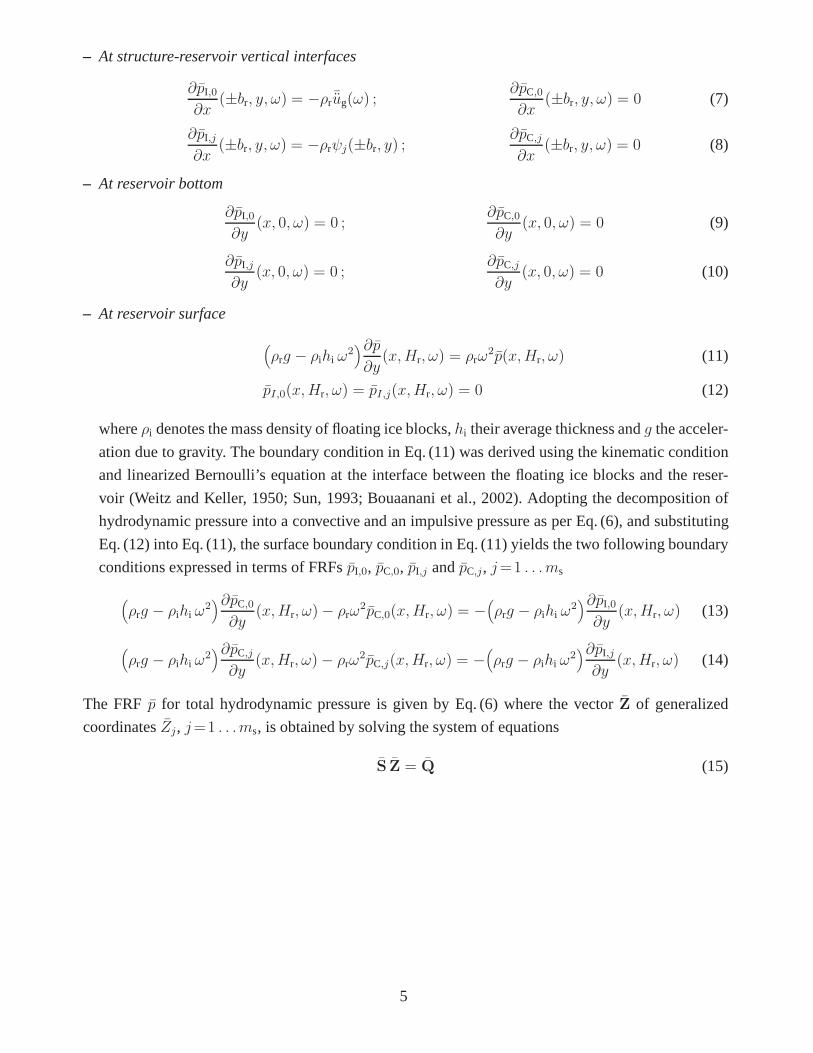
– At structure-reservoir vertical interfaces
∂pI,0
∂x(±br, y, ω) = −ρr
¯ug(ω) ;∂pC,0
∂x(±br, y, ω) = 0 (7)
∂pI,j
∂x(±br, y, ω) = −ρrψj(±br, y) ;
∂pC,j
∂x(±br, y, ω) = 0 (8)
– At reservoir bottom
∂pI,0
∂y(x, 0, ω) = 0 ;
∂pC,0
∂y(x, 0, ω) = 0 (9)
∂pI,j
∂y(x, 0, ω) = 0 ;
∂pC,j
∂y(x, 0, ω) = 0 (10)
– At reservoir surface
(ρrg − ρihi ω
2)∂p∂y
(x,Hr, ω) = ρrω2p(x,Hr, ω) (11)
pI,0(x,Hr, ω) = pI,j(x,Hr, ω) = 0 (12)
whereρi denotes the mass density of floating ice blocks,hi their average thickness andg the acceler-
ation due to gravity. The boundary condition in Eq. (11) was derived using the kinematic condition
and linearized Bernoulli’s equation at the interface between the floating ice blocks and the reser-
voir (Weitz and Keller, 1950; Sun, 1993; Bouaanani et al., 2002). Adopting the decomposition of
hydrodynamic pressure into a convective and an impulsive pressure as per Eq. (6), and substituting
Eq. (12) into Eq. (11), the surface boundary condition in Eq.(11) yields the two following boundary
conditions expressed in terms of FRFspI,0, pC,0, pI,j andpC,j, j=1 . . .ms
(ρrg − ρihi ω
2)∂pC,0
∂y(x,Hr, ω)− ρrω
2pC,0(x,Hr, ω) = −(ρrg − ρihi ω
2)∂pI,0
∂y(x,Hr, ω) (13)
(ρrg − ρihi ω
2)∂pC,j
∂y(x,Hr, ω)− ρrω
2pC,j(x,Hr, ω) = −(ρrg − ρihi ω
2)∂pI,j
∂y(x,Hr, ω) (14)
The FRFp for total hydrodynamic pressure is given by Eq. (6) where thevector Z of generalized
coordinatesZj, j=1 . . .ms, is obtained by solving the system of equations
S Z = Q (15)
5
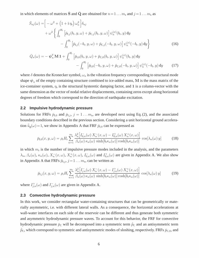
in which elements of matricesS andQ are obtained forn=1 . . .ms andj=1 . . .ms as
Snj(ω) =[− ω2 +
(1 + i ηs
)ω2n
]δnj
+ ω2
{∫ Hr
0
[pI,j(br, y, ω) + pC,j(br, y, ω)
]ψ(x)n (br, y) dy
−∫ Hr
0
[pI,j(−br, y, ω) + pC,j(−br, y, ω)
]ψ(x)n (−br, y) dy
}(16)
Qn(ω) =−ψTn M1+
∫ Hr
0
[pI,0(br, y, ω) + pC,0(br, y, ω)
]ψ(x)n (br, y) dy
−∫ Hr
0
[pI,0(−br, y, ω) + pC,0(−br, y, ω)
]ψ(x)n (−br, y) dy (17)
whereδ denotes the Kronecker symbol,ωn is the vibration frequency corresponding to structural mode
shapeψn of the empty containing structure combined to ice-added mass,M is the mass matrix of the
ice-container system,ηs is the structural hysteretic damping factor, and1 is a column-vector with the
same dimension as the vector of nodal relative displacements, containing zeros except along horizontal
degrees of freedom which correspond to the direction of earthquake excitation.
2.2 Impulsive hydrodynamic pressure
Solutions for FRFspI,0 and pI,j, j = 1 . . .ms, are developed next using Eq. (2), and the associated
boundary conditions described in the previous section. Considering a unit horizontal ground accelera-
tion ¯ug(ω)=1, we show in Appendix A that FRFpI,0 can be expressed as
pI,0(x, y, ω) = ρrHr
mr∑
n=1
λ2n[I−0,n(ω)X
−
n (x, ω)− I+0,n(ω)X+n (x, ω)
]
βn(ω) κn(ω) sinh[brκn(ω)] cosh[brκn(ω)]cos[λn(ω) y] (18)
in whichmr is the number of impulsive pressure modes included in the analysis, and the parameters
λn, βn(ω), κn(ω), X−
n (x, ω), X+n (x, ω), I
−
0,n(ω) andI+0,n(ω) are given in Appendix A. We also show
in Appendix A that FRFspI,j, j=1 . . .ms, can be written as
pI,j(x, y, ω) = ρrHr
mr∑
n=1
λ2n[I−j n(ω)X
−
n (x, ω)− I+j n(ω)X+n (x, ω)
]
βn(ω) κn(ω) sinh[brκn(ω)] cosh[brκn(ω)]cos[λn(ω) y] (19)
whereI+j,n(ω) andI−j,n(ω) are given in Appendix A.
2.3 Convective hydrodynamic pressure
In this work, we consider rectangular water-containing structures that can be geometrically or mate-
rially asymmetric, i.e. with different lateral walls. As a consequence, the horizontal accelerations at
wall-water interfaces on each side of the reservoir can be different and thus generate both symmetric
and asymmetric hydrodynamic pressure waves. To account forthis behavior, the FRF for convective
hydrodynamic pressurepC will be decomposed into a symmetric termpC and an antisymmetric term˜pC, which correspond to symmetric and antisymmetric modes of sloshing, respectively. FRFspC,0, and
6
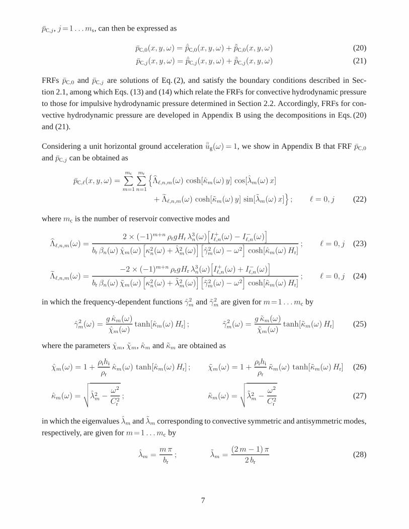
pC,j, j=1 . . .ms, can then be expressed as
pC,0(x, y, ω) = ˆpC,0(x, y, ω) + ˜pC,0(x, y, ω) (20)
pC,j(x, y, ω) = ˆpC,j(x, y, ω) + ˜pC,j(x, y, ω) (21)
FRFs pC,0 and pC,j are solutions of Eq. (2), and satisfy the boundary conditions described in Sec-
tion 2.1, among which Eqs. (13) and (14) which relate the FRFsfor convective hydrodynamic pressure
to those for impulsive hydrodynamic pressure determined inSection 2.2. Accordingly, FRFs for con-
vective hydrodynamic pressure are developed in Appendix B using the decompositions in Eqs. (20)
and (21).
Considering a unit horizontal ground acceleration¯ug(ω) = 1, we show in Appendix B that FRFpC,0
andpC,j can be obtained as
pC,ℓ(x, y, ω) =mc∑
m=1
mr∑
n=1
{Λℓ,n,m(ω) cosh[κm(ω) y] cos[λm(ω) x]
+ Λℓ,n,m(ω) cosh[κm(ω) y] sin[λm(ω) x]}; ℓ = 0, j (22)
wheremc is the number of reservoir convective modes and
Λℓ,n,m(ω) =2× (−1)m+n ρrgHr λ
3n(ω)
[I+ℓ,n(ω)− I−ℓ,n(ω)
]
br βn(ω) χm(ω)[κ2n(ω) + λ2m(ω)
] [γ2m(ω)− ω2
]cosh[κm(ω)Hr]
; ℓ = 0, j (23)
Λℓ,n,m(ω) =−2 × (−1)m+n ρrgHr λ
3n(ω)
[I+ℓ,n(ω) + I−ℓ,n(ω)
]
br βn(ω) χm(ω)[κ2n(ω) + λ2m(ω)
] [γ2m(ω)− ω2
]cosh[κm(ω)Hr]
; ℓ = 0, j (24)
in which the frequency-dependent functionsγ2m andγ2m are given form=1 . . .mc by
γ2m(ω) =g κm(ω)
χm(ω)tanh[κm(ω)Hr] ; γ2m(ω) =
g κm(ω)
χm(ω)tanh[κm(ω)Hr] (25)
where the parametersχm, χm, κm andκm are obtained as
χm(ω) = 1 +ρihi
ρrκm(ω) tanh[κm(ω)Hr] ; χm(ω) = 1 +
ρihi
ρrκm(ω) tanh[κm(ω)Hr] (26)
κm(ω) =
√√√√λ2m −ω2
C2r
; κm(ω) =
√√√√λ2m −ω2
C2r
(27)
in which the eigenvaluesλm andλm corresponding to convective symmetric and antisymmetric modes,
respectively, are given form=1 . . .mc by
λm =mπ
br; λm =
(2m− 1) π
2 br(28)
7
The natural convective symmetric and antisymmetric frequencies correspond to the frequenciesωm
andωm, respectively, that satisfy the equations
γ2m(ωm)− ω2m = 0 ; γ2m(ωm)− ω2
m = 0 (29)
form=1 . . .mc. If water is assumed incompressible, then the parametersκm andκm become frequency-
independent, and Eq. (27) simplifies to
κm = λm ; κm = λm (30)
The natural convective symmetric and antisymmetric frequenciesωm and ωm, respectively, become
also frequency-independent, and can be obtained form=1 . . .mc as
ωm =
√g κmχm
tanh(κmHr); ωm =
√g κmχm
tanh(κmHr) (31)
2.4 Time responses for a seismic loading
The generalized coordinate vectorZ is computed after substituting the impulsive and convective FRFs
into Eq. (15), then the total pressure in the frequency-domain is computed according to Eq. (6). The
time-history displacements and accelerations of a point ofthe lateral walls subjected to a ground
accelerationug(t) can be obtained as
u(x, y, t) =Ns∑
j=1
ψ(x)j (x, y)Zj(t) ; u(x, y, t) =
ms∑
j=1
ψ(x)j (x, y) Zj(t) (32)
v(x, y, t) =Ns∑
j=1
ψ(y)j (x, y)Zj(t) ; v(x, y, t) =
ms∑
j=1
ψ(y)j (x, y) Zj(t) (33)
where the time-domain generalized coordinatesZj are given by the Fourier integrals
Zj(t) =1
2π
∫∞
−∞
Zj(ω) ¯ug(ω) eiωt dω ; Zj(t) = −1
2π
∫∞
−∞
ω2Zj(ω) ¯ug(ω) eiωt dω (34)
in which ¯ug(ω) is the Fourier transform of the ground accelerationug(t)
¯ug(ω) =∫ ta
0ug(t) e−iωt dt (35)
with ta denoting the time duration of the applied accelerogram.
The time-history response for total hydrodynamic pressurep and vertical displacementζ at reservoir
surface under the effect of ground accelerationug(t) can also be obtained as
p(x, y, t) = p0(x, y, t) +ms∑
j=1
pj(x, y, t) Zj(t) (36)
8
ζ(x, t) =1
ρrgp(x,Hr, t) (37)
Based on the above relations, other quantities of interest such as shear forces or overturning moments,
can also be determined.
In the coupled systems studied, two types of damping should be accounted for to model the dissipation
of energy in the solid containing structure and in the contained fluid. A viscous damping has to be
applied to represent energy dissipation in the vibrating structure and associated impulsive modes.
A damping for convective modes is introduced to mainly account for energy dissipation within the
contained fluid, and is generally assumed to be less than0.5% for light viscosity liquids without
dissipative devices. Various design codes like the Eurocode 8 (2003) or the ACI 350.3 (2006) specify
0.5% damping for convective modes and5% damping for impulsive modes. These conservative values
are based on several studies such as (Scarsi, 1971; Martel etal., 1998; Ghaemmaghami and Kianoush,
2010). They are used in the numerical models presented next.
In the analytical formulation, damping for impulsive modesis represented by a hysteretic damping
factorηs included in Eq. (16). Damping for convective modes is accounted for through a viscous damp-
ing ξc introduced into Eqs. (38) and (39) to yield
Λℓ,n,m(ω) =2× (−1)m+n ρrgHr λ
3n(ω)
[I+ℓ,n(ω)− I−ℓ,n(ω)
]
br βn(ω) χm(ω)[κ2n(ω) + λ2m(ω)
] [γ2m(ω) + 2 i ξcω γm(ω)− ω2
]cosh[κm(ω)Hr]
(38)
Λℓ,n,m(ω) =−2 × (−1)m+n ρrgHr λ
3n(ω)
[I+ℓ,n(ω) + I−ℓ,n(ω)
]
br βn(ω) χm(ω)[κ2n(ω) + λ2m(ω)
] [γ2m(ω) + 2 i ξcω γm(ω)− ω2
]cosh[κm(ω)Hr]
(39)
for ℓ = 0, j.
The proposed method is validated in the next section througha numerical example illustrating the
dynamic response symmetric and asymmetric water-containing structures covered with floating ice
blocks.
3 Illustrative numerical example
3.1 Properties of the studied system and numerical modeling
We consider the geometrically asymmetric wall-water system illustrated in Fig. 3. It consists of two
lateral walls impounding a reservoir of heightHr=20m and a lengthLr=20m, covered with floating
ice blocks. The following properties are adopted for the constitutive material of the walls: modulus
of elasticityEs = 25GPa, Poisson’s ratioνs = 0.2, and mass densityρs = 2400 kg/m3. The water is
assumed compressible, with a velocity of pressure wavesCr = 1440m/s, and a mass densityρr =
1000 kg/m3. An ice mass densityρi = 917 kg/m3 is adopted (USACE, 2002). Although the thickness
9
of the ice blocks may vary from one point to another, an average uniform thicknesshi = 1.0m is
considered for this numerical example.
The application of the proposed method first requires the determination of the mode shapesψj ,
j=1 . . .ms, of the lateral walls without water, i.e. dry structure. Forthis purpose, both walls are dis-
cretized into 4-node plane-strain solid finite elements using the software ADINA (2010) as illustrated
in Fig. 4 (a). Fig. 5 shows the obtained first four mode shapes,i.e.ms=4, given by ADINA (2010) as
well as the corresponding frequencies and horizontal effective modal masses expressed in percentage
of total mass of the walls. Convergence studies showed thatmc = 30 convective modes are required.
A viscous damping ratioξc = 0.5% and a hysteretic damping factorηs=0.1 are applied to damp-out
convective and impulsive modes, respectively.
To validate the proposed formulation, we build a coupled fluid-structure finite element model where
both the walls and the reservoir are modeled using 4-node plane strain and 4-node potential-based
finite elements programmed in ADINA (2010), respectively. Fig. 4 (b) illustrates the finite element
mesh used. In this case, a potential-based formulation of the fluid domain is adopted (Everstine,
1981; Bouaanani and Lu, 2009). Dynamic interaction betweenthe walls and the reservoir is achieved
through fluid-structure interface elements. Beam elementswith negligible stiffness are introduced at
the reservoir surface to account for fluid-structure interaction between the reservoir and the floating
ice blocks. Two modal viscous damping values are assumed to damp-out convective and impulsive
modes, respectively: (i) a0.5% modal damping ratio is applied to the first 30 modes with low frequen-
cies corresponding to convective modes only, and (ii) a5% modal damping ratio is applied to the rest
of the modes up to the210 th.
The frequency- and time-domain dynamic responses of the wall-water system are investigated next
using the previously described analytical and finite element models shown in Figs. 4 (a) and (b).
3.2 Frequency-domain response
Fig. 6 presents the FRFs for nondimensionalized hydrodynamic pressures|p/(ρrgHr)| obtained at
points A and A’, nondimensionalized horizontal relative displacements|u/ust| at points C and C’,
whereust is the lateral static displacement under the effect of hydrostatic pressure, and nondimension-
alized vertical displacementζ/Hr at points B and B’ at reservoir surface. The results are determined
at points A, B and C located on the left wall, and points A’, B’ and C’ belonging to the right wall as
indicated in Fig. 4. The vertical positions of the points areyA = yA’ =1m, yB = yB’ =20m, yC=24m
andyC’ = 28m. The FRFs in Fig. 6 clearly show that the proposed formulation yields excellent re-
sults when compared to those obtained through finite elementmodeling whether with or without the
presence of floating ice blocks. Each frequency curve exhibits: (i) a lower frequency range part, i.e.
f60.5Hz, corresponding to convective modes, and (ii) a higher frequency range part, i.e.f>1.5Hz,
corresponding to impulsive modes. The FRFs of hydrodynamicpressures at reservoir’s bottom and the
10
lateral displacements at the top of the walls show that the presence of floating ice blocks affects dy-
namic responses corresponding to convective modes and to a much larger extent those corresponding
to the impulsive ones. As can be seen, the main effect is a decrease of resonant frequencies, a behav-
ior that can be related to the added mass from floating ice blocks. We also observe that the FRFs of
vertical displacements at reservoir surface are the most affected by the presence of ice blocks, which
mainly leads to the appearance of impulsive modes with resonant frequencies larger than1.5Hz.
The techniques described previously are applied next to determine convective and impulsive hydro-
dynamic pressure profiles corresponding to frequencies0.9 ω1, 1.1 ω1, 0.9 ω1 and1.1 ω1, whereω1
andω1 denote the natural frequencies corresponding to the first antisymmetric convective mode and
first impulsive mode, respectively. The resulting hydrodynamic profiles illustrated in Fig. 7 confirm
that the proposed formulation is in excellent agreement with the advanced finite element solution. The
profiles also reveal that the presence of ice blocks: (i) slightly decreases the amplitude of convective
hydrodynamic pressure along the height of the reservoir, and (ii) increases the amplitude of impulsive
hydrodynamic pressure, with maximum amplification observed at reservoir surface.
3.3 Time-domain response
In this section, we investigate the performance of the proposed method in assessing the seismic re-
sponse of the previously described wall-water system. The horizontal acceleration component of Impe-
rial Valley earthquake (1940) at El Centro is selected to conduct the analyses using the proposed and fi-
nite element techniques described above. Fig. 8 illustrates the first20 s of the input ground acceleration.
The obtained time-histories of nondimensionalized horizontal relative displacements|u/ust| at points
C and C’, the nondimensionalized shear forcesV/Fstat at sections A and A’, whereFstat= ρrgH2r /2
denotes the hydrostatic force, and the vertical displacementsζ at points B and B’ at reservoir surface
are shown in Figs. 9 and 10 for the reservoir with free surfaceand ice-covered, respectively. These
figures show that the time-history results given by the developed formulation and the finite element
solution are practically coincident.
We observe that the amplitudes of all the quantities studiedincrease with the presence of floating ice
blocks. This effect is maximum for the vertical displacements ζ at reservoir surface, with displace-
ments approximately 5 times larger with an ice-covered reservoir than with a free surface case. We
also note that the frequency content of the response curves is affected by the presence of ice blocks.
This is more pronounced in the response curves of reservoir surface vertical displacements as we com-
pare Figs. 9 (e) and (f) to Figs. 10 (e) and (f). Low convectivefrequencies dominate indeed the free
surface reservoir dynamic response as anticipated from theFRF of reservoir surface vertical displace-
ment shown in Fig. 6 (e), which explains the predominant longperiod oscillations in the time-domaine
response of free surface vertical displacements in Figs. 9 (e) and (f). We also note the obvious oppo-
sition of phase of vertical displacements at points B and B’,which originates from predominant first
antisymmetric sloshing mode. On the other hand, Fig. 6 (f) shows that the FRF of vertical displacement
11
of ice-covered reservoir surface also contains low frequency convective modes, but more importantly
impulsive modes with resonant frequencies larger than1.5Hz, similarly to the FRFs of hydrodynamic
pressure or lateral displacements in Figs. 6 (a) to (d). These impulsive modes are predominant in the
time-domain response of ice-covered reservoir surface vertical displacements shown in Figs. 9 (e) and
(f), which explains the approximate resemblance of their time-history signature to that of lateral dis-
placements and base shears in Figs. 9 (a) to (d), also dominated by impulsive modes. We see from the
latter figures that maximum displacements at top of container lateral walls are amplified by about1.5
times due to the presence of floating ice blocks, while the shear force at the base of the walls is not
significantly affected.
Finally, the proposed formulation is used to illustrate theeffect of asymmetry of the previous ice-
covered water-containing structure on its dynamic response. For this purpose, we consider a symmet-
ric rectangular water-containing structure made by replacing the right wall of the asymmetric structure
in Fig. 3 by its3m-thick and24m-high rectangular left wall. The dimensions of the reservoir are the
same as the asymmetric wall-water system. The symmetric water-containing structure is subjected
to the same earthquake as previously. The time-histories ofnondimensionalized horizontal displace-
ments|u/ust| at point C, as well as vertical displacementsζ at points B and B’ at reservoir surface
obtained using the developed method are illustrated in Fig.11 for the symmetric and asymmetric
water-containing structures. The results in Figs. 11 (a) and (b) show that asymmetry has a minor effect
of the structural response of the walls either with or without ice blocks. The vertical displacements of
reservoir surface at point B are also practically insensitive to asymmetry with or without ice blocks as
observed in Figs. 11 (c) and (d). Figs. 11 (e) and (f) reveal however that the vertical displacements of
reservoir surface at point B’ are affected by asymmetry under free surface conditions, and to a much
larger extent when the reservoir is covered by ice blocks. This result emphasizes that, for the particular
water-containing structures studied, the presence of ice blocks increases the impact of asymmetry on
hydrodynamic response indicators such as displacement fluctuations at reservoir surface.
4 Conclusions
This paper presented a new formulation to investigate the effects of floating ice blocks on seismically-
excited rectangular water-containing structures. The proposed method is based on a sub-structuring
approach, where the flexible containing structure and ice-added mass are modeled using finite ele-
ments, while hydrodynamic effects are modeled analytically through interaction forces at the water-
structure and water-ice interfaces, thus eliminating the need for reservoir finite element discretization.
In addition to accounting for the influence of floating ice blocks and container walls’ flexibility, the
developed frequency- and time-domain techniques also include the effects of container asymmetry as
well as the coupling between convective and impulsive components of hydrodynamic pressure. The
application of the proposed formulation is illustrated through a numerical example illustrating the dy-
namic response of an asymmetric water-containing structure covered with floating ice blocks, as well
as that of an equivalent symmetric structure containing a reservoir with the same dimensions. The ob-
12
tained time- and frequency-domain responses showed that the proposed formulation yields excellent
results when compared to those from coupled fluid-structurefinite element modeling either with or
without the presence of floating ice blocks. For the water-containing structures studied, we observed
that the presence of floating ice blocks mainly affects dynamic responses corresponding to convective
and impulsive modes as follows: (i) a slight decrease of convective frequencies and a more important
decrease of impulsive ones, mainly due to the added mass fromthe floating ice blocks; (ii) a slight de-
crease of the amplitude of convective hydrodynamic pressure along the height of the reservoir; (iii) an
increase of the amplitude of impulsive hydrodynamic pressure, with maximum amplification observed
at reservoir surface; (iv) an increase of the amplitudes of displacements, shear forces and, in particular,
vertical sloshing displacements at reservoir surface.
List of symbols
Abbreviations
FRF frequency response function
Symbols
An,0,An,j, A′
n,0 andA′
n,j coefficients used for mathematical derivations in AppendixA
Bm,0,Bm,j ,B′
m,0 andB′
m,j coefficients used for mathematical derivations in AppendixB
ag amplitude of harmonic ground acceleration
¯ug Fourier transform of ground accelerationug
br half-length of the reservoir
Cr compression wave velocity within the reservoir
ℓ index referring to rigid body motion effects whenℓ=0 and to lateral vibrations
along structural modej whenℓ=j
Es modulus of elasticity of the containing structure
Fstat hydrostatic force
g acceleration due to gravity
hi average thickness of the floating ice blocks
Hr height of the reservoir
13
I−0,n andI+0,n parameters given by Eq. (A11) forn=1 . . . mr
I−j,n andI+j,n parameters given by Eqs. (A12) and (A13) forj=1 . . . ms andn=1 . . . mr
Lr length of the reservoir
M mass matrice of the ice-container system
mc number of reservoir convective modes
mr number of impulsive pressure reservoir modes included in the analysis
ms number of structural mode shapes included in the analysis
p andb hydrodynamic pressure and corresponding FRF, respectively
p0 FRF for hydrodynamic pressure due to rigid body motion of thecontaining
structure subjected to ground acceleration¯ug
pj FRF for hydrodynamic pressure due to horizontal ground accelerations
ψ(x)j (−br, y) andψ(x)
j (br, y) of the lateral walls vibrating along structural mode
j
pI andpC impulsive and convective components of hydrodynamic pressure FRFb
pI,0 andpC,0 impulsive and convective components of hydrodynamic pressure FRFb0
pI,j andpC,j impulsive and convective components of hydrodynamic pressure FRFbj
ˆpC and ˜pC symmetric and antisymmetric components of convective hydrodynamic pres-
sure FRFpC, respectively
ˆpC,0 and ˜pC,0 symmetric and antisymmetric components of convective hydrodynamic pres-
sure FRFpC,0, respectively
ˆpC,j and ˜pC,j symmetric and antisymmetric components of convective hydrodynamic pres-
sure FRFpC,j , respectively
Q andQn vector in Eq. (15) and its elements given by Eq. (17) forn=1 . . . ms, respec-
tively
S andSnj matrix in Eq. (15) and its elements given by Eq. (16) forn = 1 . . . ms and
j=1 . . . ms, respectively
t time variable
ta time duration of the applied accelerogram
14
x andy horizontal and vertical axes of Cartesian coordinate system, respectively
X−
n andX+n parameters given by Eq. (A14) forn=1 . . . mr
u andv time-history response of horizontal and vertical structural displacements, re-
spectively
ust lateral static displacement under the effect of hydrostatic pressure
u andv FRFs of horizontal and vertical structural displacements,respectively
ug time-history of ground acceleration
¯u and ¯v FRFs of horizontal and the vertical structural accelerations, respectively
V shear force
Z andZj vector of generalized coordinates andj th generalized coordinate, respectively
1 column-vector with the same dimension as the vector of nodalrelative dis-
placements, containing zeros except along horizontal degrees of freedom
which correspond to the direction of earthquake excitation
βn parameter given by Eq. (A10) forn=1 . . . mr
γm andγm parameters given by Eq. (25) form=1 . . . mc
δ Kronecker symbol
ζ vertical displacement at reservoir surface
ηs structural hysteretic damping factor
κn parameter given by Eq. (A3) forn=1 . . . mr
κm andκm parameters given by Eq. (27) form=1 . . . mc
λn eigenvalue given by Eq. (A3) forn=1 . . . mr
λm andλm eigenvalues given by Eq. (28) form=1 . . . mc
Λℓ,n,m andΛℓ,n,m parameters given by Eqs. (38) and (39), respectively, forℓ=0, j, m=1 . . . mc
andn=1 . . . mr
∇2 Laplace differential operator
νs Poisson’s ratio of the containing structure
15
ξc viscous damping associated with convective modes
ρi mass density of floating ice blocks
ρr mass density of water
ρs mass density of the containing structure
ψn n th mode shape of the empty containing structure combined to ice-added mass
χm andχm parameters given by Eq. (26) form=1 . . . mc
ψ(x)j andψ(y)
j x- andy-components of thej th structural mode shape, respectively
ω exciting frequency
ωn vibration frequency corresponding to structural mode shapeψn of the empty
containing structure combined to ice-added mass
ωm m th impulsive frequency
ωm andωm m th convective symmetric and antisymmetric frequencies, respectively
16

Acknowledgements
The authors would like to acknowledge the financial support of the Natural Sciences and Engineering
Research Council of Canada (NSERC) and the Quebec Research Funds for Natural Sciences and
Engineering (FRQNT).
17
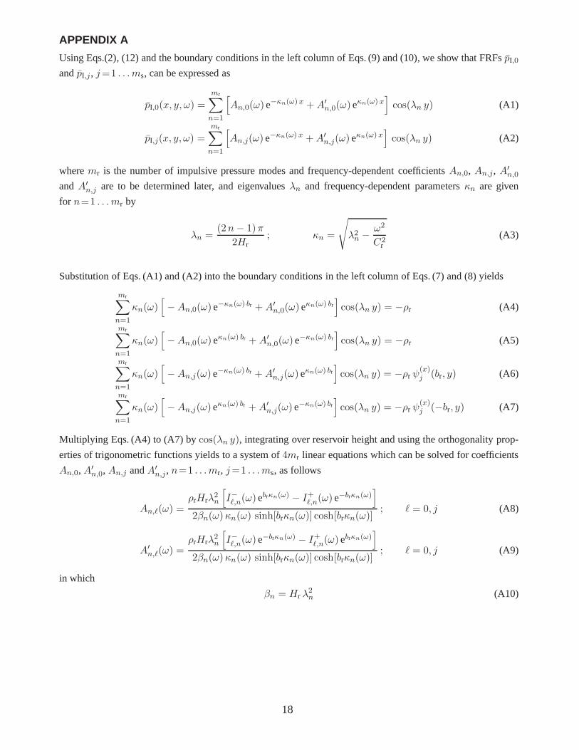
APPENDIX A
Using Eqs.(2), (12) and the boundary conditions in the left column of Eqs. (9) and (10), we show that FRFspI,0
andpI,j, j=1 . . . ms, can be expressed as
pI,0(x, y, ω) =
mr∑
n=1
[An,0(ω)e−κn(ω) x +A′
n,0(ω)eκn(ω) x]cos(λn y) (A1)
pI,j(x, y, ω) =mr∑
n=1
[An,j(ω)e−κn(ω) x +A′
n,j(ω)eκn(ω) x]cos(λn y) (A2)
wheremr is the number of impulsive pressure modes and frequency-dependent coefficientsAn,0, An,j, A′
n,0
andA′
n,j are to be determined later, and eigenvaluesλn and frequency-dependent parametersκn are given
for n=1 . . . mr by
λn =(2n− 1)π
2Hr; κn =
√λ2n −
ω2
C2r
(A3)
Substitution of Eqs. (A1) and (A2) into the boundary conditions in the left column of Eqs. (7) and (8) yields
mr∑
n=1
κn(ω)[−An,0(ω)e−κn(ω) br +A′
n,0(ω)eκn(ω) br
]cos(λn y) = −ρr (A4)
mr∑
n=1
κn(ω)[−An,0(ω)eκn(ω) br +A′
n,0(ω)e−κn(ω) br
]cos(λn y) = −ρr (A5)
mr∑
n=1
κn(ω)[−An,j(ω)e−κn(ω) br +A′
n,j(ω)eκn(ω) br
]cos(λn y) = −ρr ψ
(x)j (br, y) (A6)
mr∑
n=1
κn(ω)[−An,j(ω)eκn(ω) br +A′
n,j(ω)e−κn(ω) br
]cos(λn y) = −ρr ψ
(x)j (−br, y) (A7)
Multiplying Eqs. (A4) to (A7) bycos(λn y), integrating over reservoir height and using the orthogonality prop-
erties of trigonometric functions yields to a system of4mr linear equations which can be solved for coefficients
An,0,A′
n,0, An,j andA′
n,j, n=1 . . . mr, j=1 . . . ms, as follows
An,ℓ(ω) =ρrHrλ
2n
[I−ℓ,n(ω)ebrκn(ω) − I+ℓ,n(ω)e−brκn(ω)
]
2βn(ω)κn(ω) sinh[brκn(ω)] cosh[brκn(ω)]; ℓ = 0, j (A8)
A′
n,ℓ(ω) =ρrHrλ
2n
[I−ℓ,n(ω)e−brκn(ω) − I+ℓ,n(ω)ebrκn(ω)
]
2βn(ω)κn(ω) sinh[brκn(ω)] cosh[brκn(ω)]; ℓ = 0, j (A9)
in which
βn = Hr λ2n (A10)
18
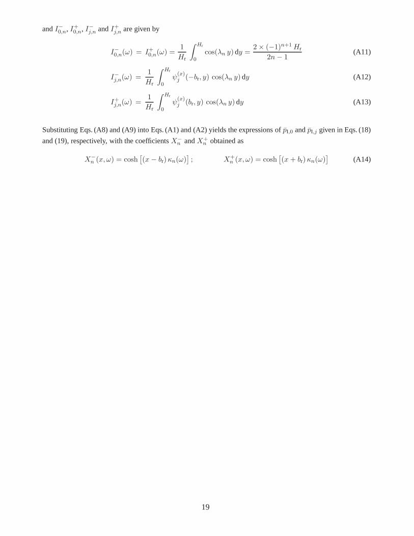
andI−0,n, I+0,n, I−j,n andI+j,n are given by
I−0,n(ω) = I+0,n(ω) =1
Hr
∫ Hr
0cos(λn y)dy =
2× (−1)n+1Hr
2n− 1(A11)
I−j,n(ω) =1
Hr
∫ Hr
0ψ(x)j (−br, y) cos(λn y)dy (A12)
I+j,n(ω) =1
Hr
∫ Hr
0ψ(x)j (br, y) cos(λn y)dy (A13)
Substituting Eqs. (A8) and (A9) into Eqs. (A1) and (A2) yields the expressions ofpI,0 andpI,j given in Eqs. (18)
and (19), respectively, with the coefficientsX−
n andX+n obtained as
X−
n (x, ω) = cosh[(x− br)κn(ω)
]; X+
n (x, ω) = cosh[(x+ br)κn(ω)
](A14)
19
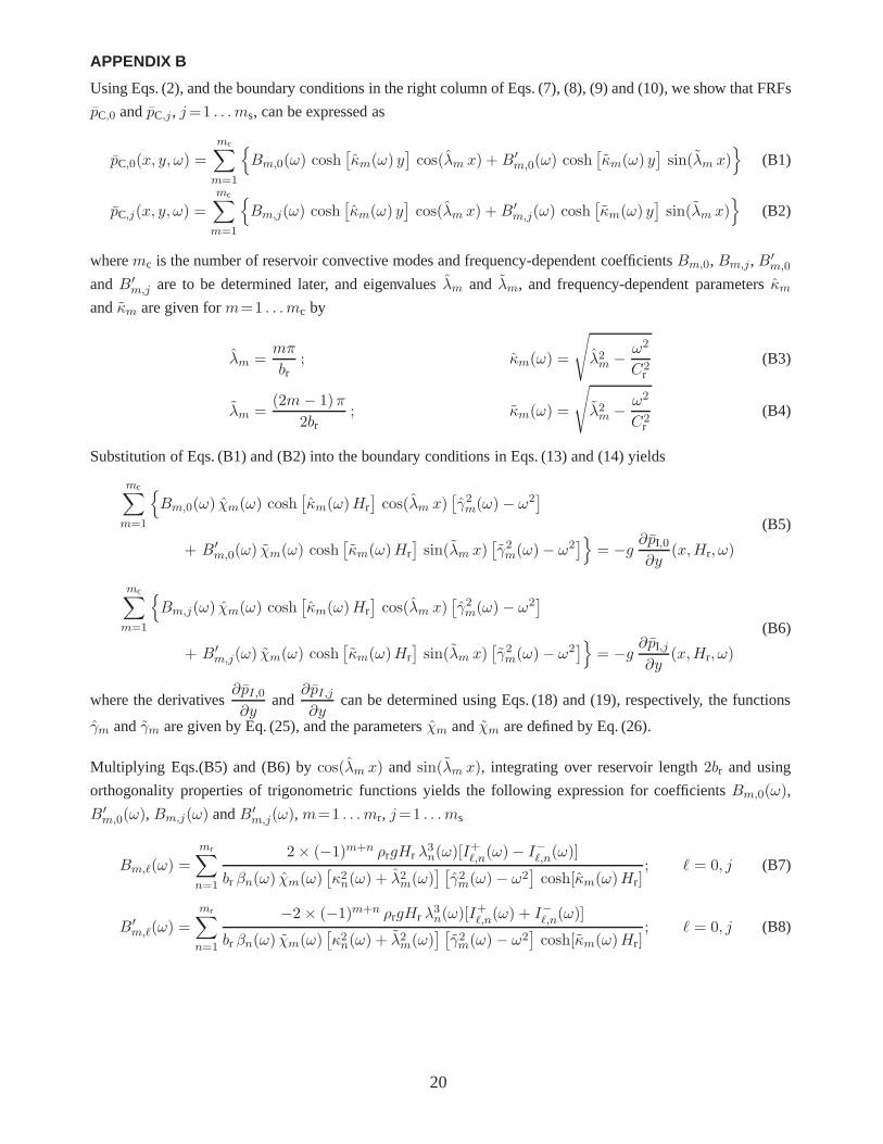
APPENDIX B
Using Eqs. (2), and the boundary conditions in the right column of Eqs. (7), (8), (9) and (10), we show that FRFs
pC,0 andpC,j, j=1 . . . ms, can be expressed as
pC,0(x, y, ω) =
mc∑
m=1
{Bm,0(ω) cosh
[κm(ω) y
]cos(λm x) +B′
m,0(ω) cosh[κm(ω) y
]sin(λm x)
}(B1)
pC,j(x, y, ω) =
mc∑
m=1
{Bm,j(ω) cosh
[κm(ω) y
]cos(λm x) +B′
m,j(ω) cosh[κm(ω) y
]sin(λm x)
}(B2)
wheremc is the number of reservoir convective modes and frequency-dependent coefficientsBm,0,Bm,j,B′
m,0
andB′
m,j are to be determined later, and eigenvaluesλm and λm, and frequency-dependent parametersκm
andκm are given form=1 . . . mc by
λm =mπ
br; κm(ω) =
√λ2m −
ω2
C2r
(B3)
λm =(2m− 1)π
2br; κm(ω) =
√λ2m −
ω2
C2r
(B4)
Substitution of Eqs. (B1) and (B2) into the boundary conditions in Eqs. (13) and (14) yields
mc∑
m=1
{Bm,0(ω) χm(ω) cosh
[κm(ω)Hr
]cos(λm x)
[γ2m(ω)− ω2
]
+ B′
m,0(ω) χm(ω) cosh[κm(ω)Hr
]sin(λm x)
[γ2m(ω)− ω2
]}= −g
∂pI,0
∂y(x,Hr, ω)
(B5)
mc∑
m=1
{Bm,j(ω) χm(ω) cosh
[κm(ω)Hr
]cos(λm x)
[γ2m(ω)− ω2
]
+ B′
m,j(ω) χm(ω) cosh[κm(ω)Hr
]sin(λm x)
[γ2m(ω)− ω2
]}= −g
∂pI,j
∂y(x,Hr, ω)
(B6)
where the derivatives∂pI,0
∂yand
∂pI,j
∂ycan be determined using Eqs. (18) and (19), respectively, the functions
γm andγm are given by Eq. (25), and the parametersχm andχm are defined by Eq. (26).
Multiplying Eqs.(B5) and (B6) bycos(λm x) and sin(λm x), integrating over reservoir length2br and using
orthogonality properties of trigonometric functions yields the following expression for coefficientsBm,0(ω),
B′
m,0(ω), Bm,j(ω) andB′
m,j(ω),m=1 . . . mr, j=1 . . . ms
Bm,ℓ(ω) =
mr∑
n=1
2× (−1)m+n ρrgHr λ3n(ω)[I
+ℓ,n(ω)− I−ℓ,n(ω)]
br βn(ω) χm(ω)[κ2n(ω) + λ2m(ω)
] [γ2m(ω)− ω2
]cosh[κm(ω)Hr]
; ℓ = 0, j (B7)
B′
m,ℓ(ω) =
mr∑
n=1
−2× (−1)m+n ρrgHr λ3n(ω)[I
+ℓ,n(ω) + I−ℓ,n(ω)]
br βn(ω) χm(ω)[κ2n(ω) + λ2m(ω)
] [γ2m(ω)− ω2
]cosh[κm(ω)Hr]
; ℓ = 0, j (B8)
20
References
ACI committee 350. 2006. Seismic design of liquid-containing concrete structures and commentary (ACI 350.3-06).
ADINA Theory and Modeling Guide., 2010. Report ARD 06-7. ADINA R & D, Inc.
Balendra, T., Ang, K.K., Paramasivam, P. Lee, S.V., 1982. Seismic design of flexible cylindrical liquid storagetanks. Earthquake Engineering and Structural Dynamics 10(3), 477–496.
Bouaanani, N., Paultre, P., Proulx, J., 2002. Two-dimensional modelling of ice cover effects for the dynamicanalysis of concrete gravity dams. Earthquake Engineeringand Structural Dynamics 31, 2083–2102.
Bouaanani, N., Paultre, P., 2005. A new boundary condition for energy radiation in covered reservoirs usingBEM. Engineering Analysis with Boundary Elements 29, 903—911.
Bouaanani, N., Lu, F.Y., 2009. Assessment of potential-based fluid finite elements for seismic analysis of dam-reservoir systems. Journal of Computers and Structures 87,206–224.
Croteau, P., 1983. Dynamic interactions between floating ice and offshore structures. University of California,Berkeley, Calif. Report No. UCB/EERC-83/06.
Chopra, A.K., 1967. Reservoir-dam interaction during earthquake. Bull. Seismological Soc. of America 57,675–687.
Chopra, A.K., 1968. Earthquake behavior of reservoir-dam systems. Journal of the Eng. Mech. Div., ASCE 94,1475–1500.
Chopra, A.K., 1970. Earthquake response of concrete gravity dams. Journal of the Eng. Mech. Div., ASCE 96,443–454.
Cammaert, A.B., Muggeridge, D.B., 1988. Ice interaction with offshore structures. Van Nostrand Reinhold, NewYork.
Everstine, G.C., 1981. A symmetric potential formulation for fluid-structure interaction. Journal of Sound andVibration 79(1), 157–160.
Fenves, G., Chopra, A.K., 1984. Earthquake analysis and response of concrete gravity dams. Earthquakeengineering research center.
Fisher, F.D., Rammerstorfer, F.G., 1999. A refined analysisof sloshing effects in seismically excited tanks.International Journal of Pressure Vessels and Piping 76, 693–709.
Ghaemmaghami, A.R., Kianoush, M.R., 2010. Effect of wall flexibility on dynamic response of concreterectangular liquid storage tanks under horizontal and vertical ground motions 136(4), 441–451.
J. Struct. Eng., 136(4), 441–451.
Gupta, R.K., Hutchinson, G.L., 1990. Effects of wall flexibility on the dynamic response of liquid storage tanks.Engineering Structures 13, 253–267.
Haroun, M.A., Housner, G.W., 1982. Complications in free vibration analysis of tanks. Proc., ASCE EngineeringMechanics Division 108(5), 801–818.
21
Haroun, M.A., 1980. Dynamic analyses of liquid storage tanks. EERL80-04, Earthquake Engineering ResearchLaboratory, California Institute of Technology.
Hall, J.F. (ed)., 1995. Northridge Earthquake of January 17, 1994: Reconnaissance Report. Earthquake Spectra,Supplement C to Volume 11, Earthquake Engineering ResearchInstitute, Oakland, CA.
Hanson, R.D., 1973. Behavior of storage tanks, the great Alaska earthquake of 1964. Proc., National Academyof Science, Washington, D.C., 331–339.
Haroun, M.A., 1983. Vibration studies and tests of liquid storage tanks. Earthquake Engineering and StructuralDynamics 11(2), 179–206.
Housner, G.W., 1957. Dynamic pressures on accelerated fluidcontainers. Bulletin of the Seismological Societyof America 47, 15–35.
Housner, G.W., 1963. The dynamic behavior of water tanks. Bulletin of the seismological society of america53(2), 381–387.
Haroun, M.A., Housner, G.W., 1981a. Seismic design of liquid storage tanks. Journal of Techniqcal Council ofASCE 107, 191–207.
Haroun, M.A., Housner, G.W., 1981b. Earthquake response ofdeformable liquid storage tanks. Journal ofApplied Mechanics 48(2), 411–418.
Jacobsen, L.S., 1949. Impulsive hydrodynamics of fluid inside a cylindrical tank and of fluid surrounding acylindrical pier. Bulletin of the Seismological Society ofAmerica 39(3), 189–204.
Jacobsen, L.S., Ayre, R.S., 1951. Hydrodynamic experiments with rigid cylindrical tnaks subjected to transientmotions. Bulletin of the Seismological Society of America 41, 313–346.
Kana, D.D., 1979. Seismic response of flexible cylindrical liquid storage tanks. Nuclear Engineering and Design52(1), 185–199.
Kiyokawa, T., Inada, H., 1989. Hydrodynamic forces acting on axisymmetric bodies immersed in ice coveredsea during earthquakes. Proceedings of 8th International Conference on Offshore Mechanics and ArcticEngineering, The Hague, The Netherlands, 19-23 March 1989.American Society of Mechanical Engineers,New York, 153–159.
Koketsu, K., Hayatama, K., Furumura, T., Ikegami, Y., Akiyama, S., 2005. Damaging long-period groundmotions from the 2003 Mw 8.3 Tokachi-Oki, Japan earthquake.Seismological Research Letters 76(1),58–64.
Krausmann, E., Renni, E., Campedel, M. and Cozzani, V., 2011. Indistrial accidents triggered by earthquakes,floods and lightening: lessons learned from a database analysis. Natural Hazards 59, 285–300.
Malhotra, P.K., Norwood, M.A., Wieland, M., 2000. Simple procedure for seismic analysis of liquid-storagetanks. IABSE Structural Engineering International 3, 197–201.
Martel, C., Nicolas, J.A., Vega, J.M., 1998. Surface-wave damping in a brinmful circular cylinder, J. Fluid Mech.360, 213–228.
22
Miura, F., Nozawa, I., Sakaki, N., Hirano, K., 1988. Dynamicstability of an offshore structure surroundedby thick ice during strong earthquake motions. Proceedingsof the 9th World Conference on EarthquakeEngineering, Tokyo-Kyoto, Japan, August 1988. Japan Association for earthquake Disaster Prevention,Yokyo, Japan. 465–470.
Paultre, P., Proulx, J., and Carbonneau, C. 2002. An experimental evaluation of ice cover effects on the dynamicbehaviour of a concrete gravity dam. Earthquake Engineering and Structural Dynamics 31, 2067—2082.
Scarsi, G., 1971. Natural frequencies of viscous liquids inrectangular tanks, Meccanica 6(4), 223–234.
Steinberg, L.J., Cruz, A.M., 2004. When natural and technological disasters collide: Lessons from the Turkeyearthquake of August 17, 1999. Natural Hazards Review 5(3),121–130.
Steinbrugge, K. V., Flores, R., 1963. The Chilean earthquakes of May, 1960: A structural engineering viewpoint.Bulletin of the Seismological Society of America 53(2), 225–307.
Sun, K., 1993. Effects of ice layer on hydrodynamic pressureof structures. ASCE Journal of Cold RegionsEngineers 7(3), 63–76.
US Army Corsp of Engineers, 2002. Ice Engineering - EngineerManual 1110-2-1612. US Army Corps ofEngineers, Washington DC. 30 October 2002
Veletsos, A.S., Tang, Y., 1990. Soil-structure interaction effects for laterally excited liquid-storage tanks.Earthquake Engrg. Struct. Dyn. 19, 473–496.
Veletsos, A.S., 1974. Seismic effects in flexible liquid storage tanks. Proc. of Fifth World Conf. on EarthquakeEng., 630–639.
Veletsos, A.S., Yang, J.Y., 1976. Dynamics of fixed-base liquid storage tanks. US-Japan Seminar for EarthquakeEngineering Research, Tokyo, Japan, 317–341.
Veletsos, A.S., Yang, J.Y., 1977. Earthquake response of liquid storage tanks. Proc. Second EMD SpecialtyConference, ASCE, Raleigh, NC, 1–24.
Weitz, M., Keller, J., 1950. Reflection of water waves from foating ice in water of finite depth. Communicationson Pure and Applied Mathematics 3:305-–318.
Werner, P.W., Sundquit, K.J., 1949. On hydrodynamic earthquake effects. Transactions of AmericanGeophysical Union 30(5), 636–657.
Westergaard, H.M.,1933. Water pressures on dams during earthquakes. Transactions, ASCE 98, 418–472.
23
List of figures
Fig. 1: General geometry of the studied ice-water-structure systems.
Fig. 2: Sub-structuring approach: (a) Containing structure and ice-added mass; (b) reservoir model.
Fig. 3: Geometry of the wall-water system studied in the numerical example.
Fig. 4: Numerical models: (a) Analytical model of the fluid domain and finite element model of thedry containing structure; (b) Coupled fluid-structure interaction finite element model.
Fig. 5: First four mode shapes and corresponding frequencies and effective modal masses of the emptywall-water-ice system: (a) Walls without ice-added mass effects; (b) Walls with ice-added masseffect.
Fig. 6: Frequency response of nondimensionalized hydrodynamic pressures and displacements of theasymmetric wall-water system: (a) Hydrodynamic pressureswithout ice cover; (b) Hydrody-namic pressures with ice cover; (c) Horizontal displacements without ice cover; (d) Horizontaldisplacements with ice cover; (e) Vertical displacement ofreservoir free surface; (f) Verticaldisplacement of ice-covered reservoir surface.
Fig. 7: Nondimensionalized hydrodynamic pressure profileson the walls of the of the asymmetricwall-water system: (a) Convective hydrodynamic pressureswithout ice cover; (b) Impulsivehydrodynamic pressures without ice cover; (c) Convective hydrodynamic pressures with icecover; (d) Impulsive hydrodynamic pressures with ice cover.
Fig. 8: Horizontal acceleration component of Imperial Valley earthquake (1940) at El Centro.
Fig. 9: Time-history response of the asymmetric wall-watersystem without ice: (a) Nondimension-alized displacement at point C; (b) Nondimensionalized displacement at point C’; (c) Nondi-mensionalized shear force at section A; (d) Nondimensionalized shear force at section A’; (e)Nondimensionalized vertical displacement of water at point B; (f) Nondimensionalized verti-cal displacement of water at point B’.
Fig. 10: Time-history response of the asymmetric wall-water system with ice: (a) Nondimensionalizeddisplacement at point C; (b) Nondimensionalized displacement at point C’; (c) Nondimen-sionalized shear force at section A; (d) Nondimensionalized shear force at section A’; (e)Nondimensionalized vertical displacement of water at point B; (f) Nondimensionalized ver-tical displacement of water at point B’.
Fig. 11: Time-history responses of the symmetric and asymmetric wall-water systems: (a) Nondimen-sionalized displacement at point C without ice; (b) Nondimensionalized displacement at pointC with ice; (c) Nondimensionalized vertical displacement of water at point B without ice; (d)Nondimensionalized vertical displacement of water at point B with ice; (e) Nondimensional-ized vertical displacement of water at point B’ without ice;(f) Nondimensionalized verticaldisplacement of water at point B’ with ice.
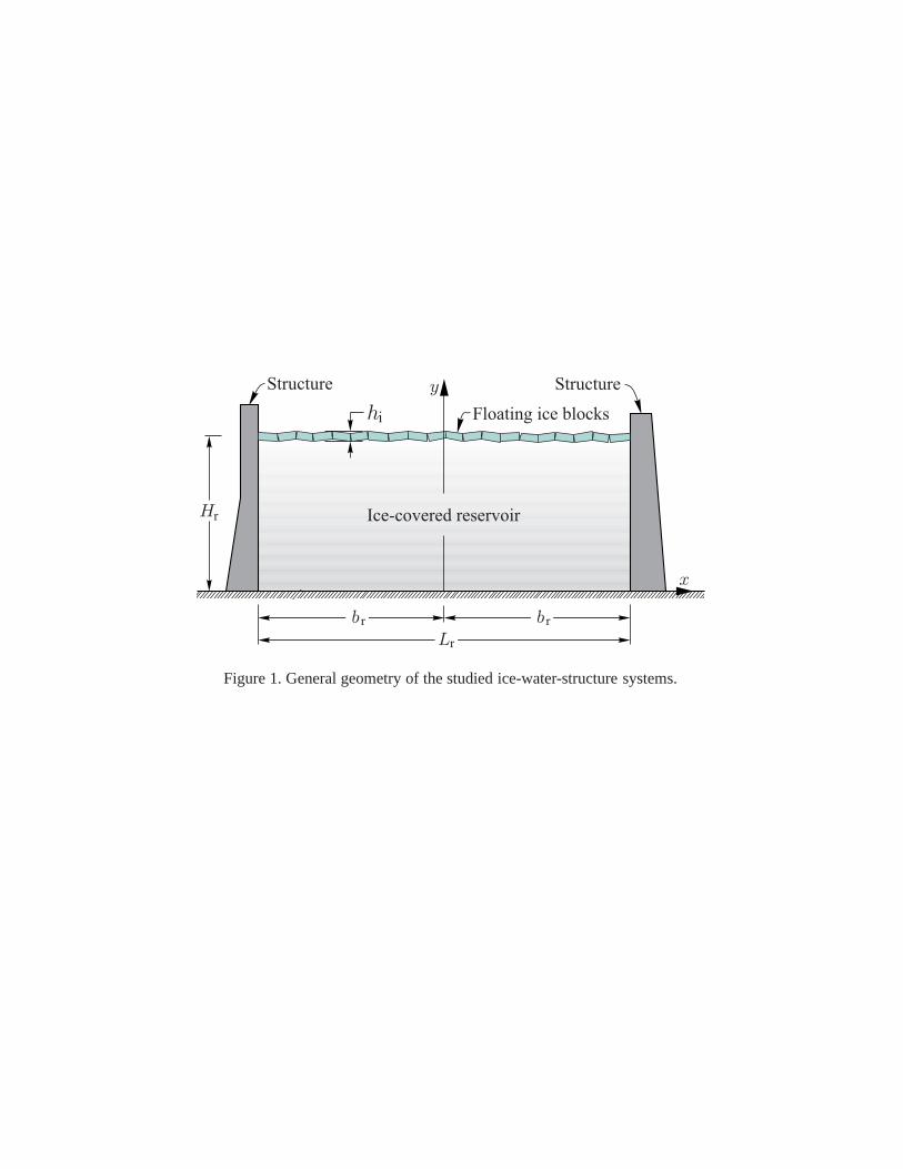
Figure 1. General geometry of the studied ice-water-structure systems.
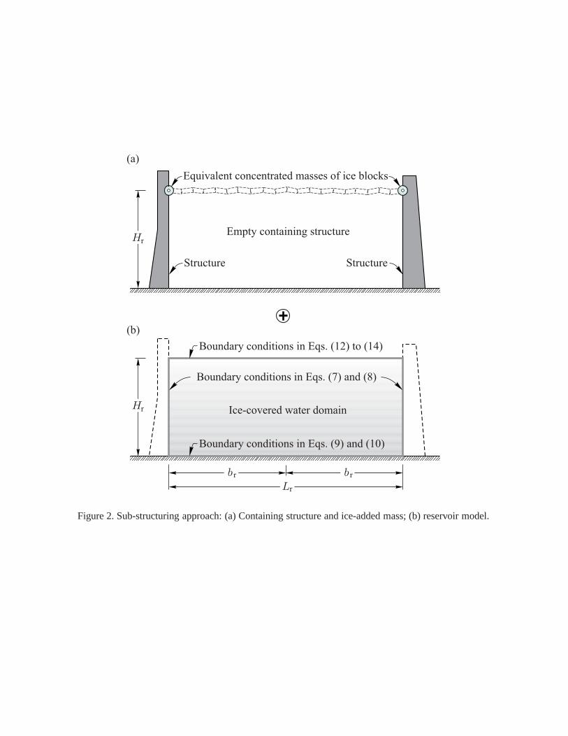
Figure 2. Sub-structuring approach: (a) Containing structure and ice-added mass; (b) reservoir model.
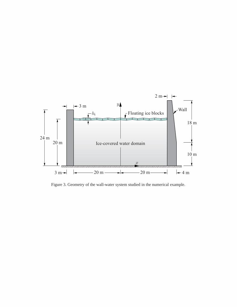
Figure 3. Geometry of the wall-water system studied in the numerical example.
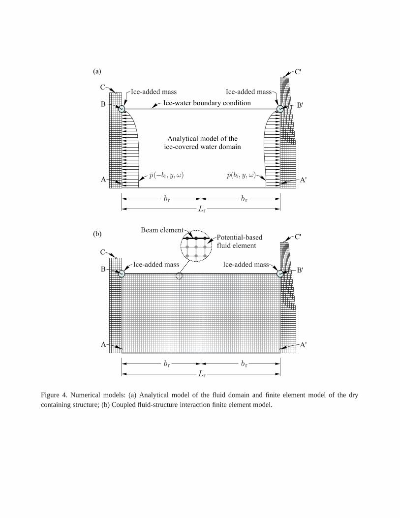
Figure 4. Numerical models: (a) Analytical model of the fluiddomain and finite element model of the drycontaining structure; (b) Coupled fluid-structure interaction finite element model.
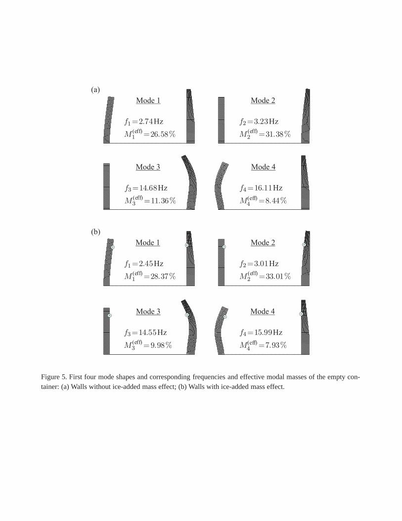
Figure 5. First four mode shapes and corresponding frequencies and effective modal masses of the empty con-tainer: (a) Walls without ice-added mass effect; (b) Walls with ice-added mass effect.
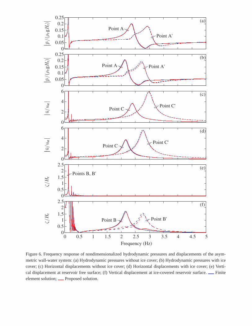
Figure 6. Frequency response of nondimensionalized hydrodynamic pressures and displacements of the asym-metric wall-water system: (a) Hydrodynamic pressures without ice cover; (b) Hydrodynamic pressures with icecover; (c) Horizontal displacements without ice cover; (d)Horizontal displacements with ice cover; (e) Verti-cal displacement at reservoir free surface; (f) Vertical displacement at ice-covered reservoir surface.Finiteelement solution; Proposed solution.
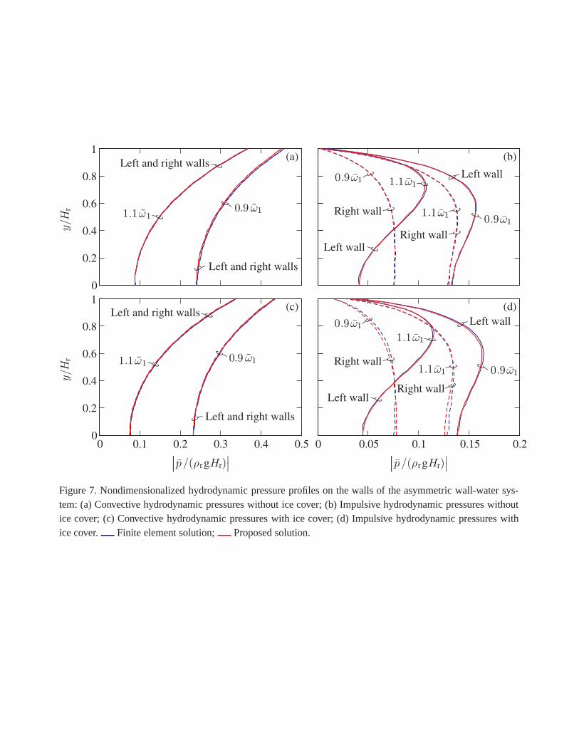
Figure 7. Nondimensionalized hydrodynamic pressure profiles on the walls of the asymmetric wall-water sys-tem: (a) Convective hydrodynamic pressures without ice cover; (b) Impulsive hydrodynamic pressures withoutice cover; (c) Convective hydrodynamic pressures with ice cover; (d) Impulsive hydrodynamic pressures withice cover. Finite element solution; Proposed solution.
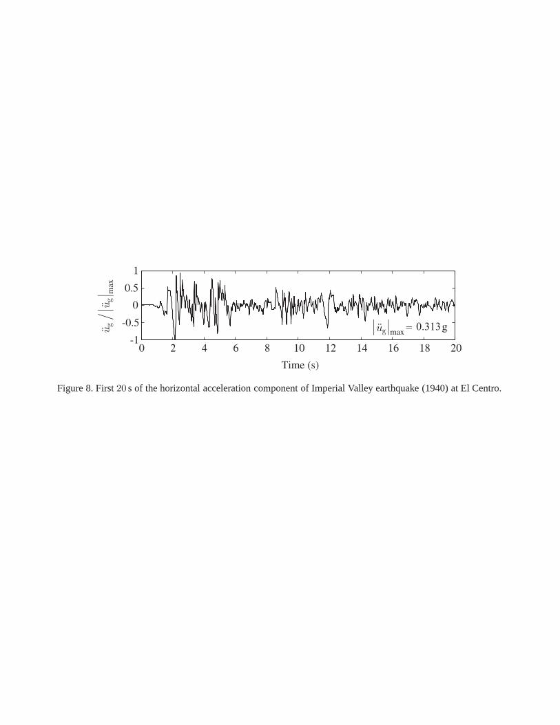
Figure 8. First20 s of the horizontal acceleration component of Imperial Valley earthquake (1940) at El Centro.
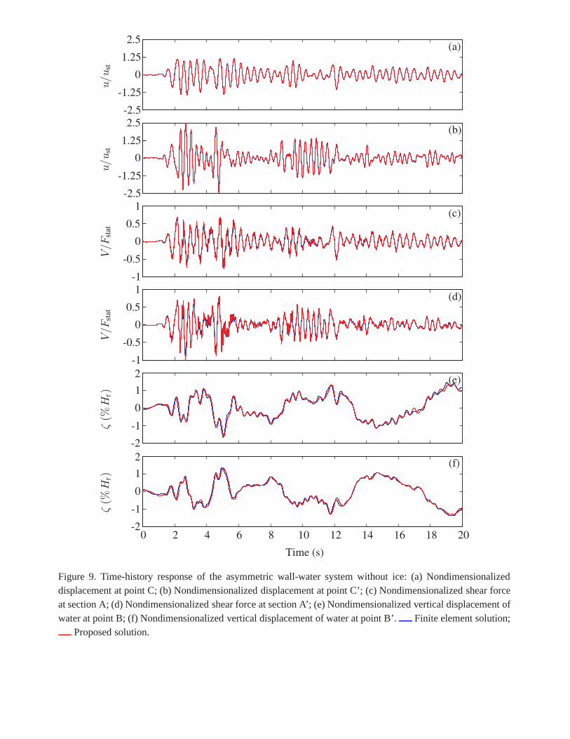
Figure 9. Time-history response of the asymmetric wall-water system without ice: (a) Nondimensionalizeddisplacement at point C; (b) Nondimensionalized displacement at point C’; (c) Nondimensionalized shear forceat section A; (d) Nondimensionalized shear force at sectionA’; (e) Nondimensionalized vertical displacement ofwater at point B; (f) Nondimensionalized vertical displacement of water at point B’. Finite element solution;
Proposed solution.
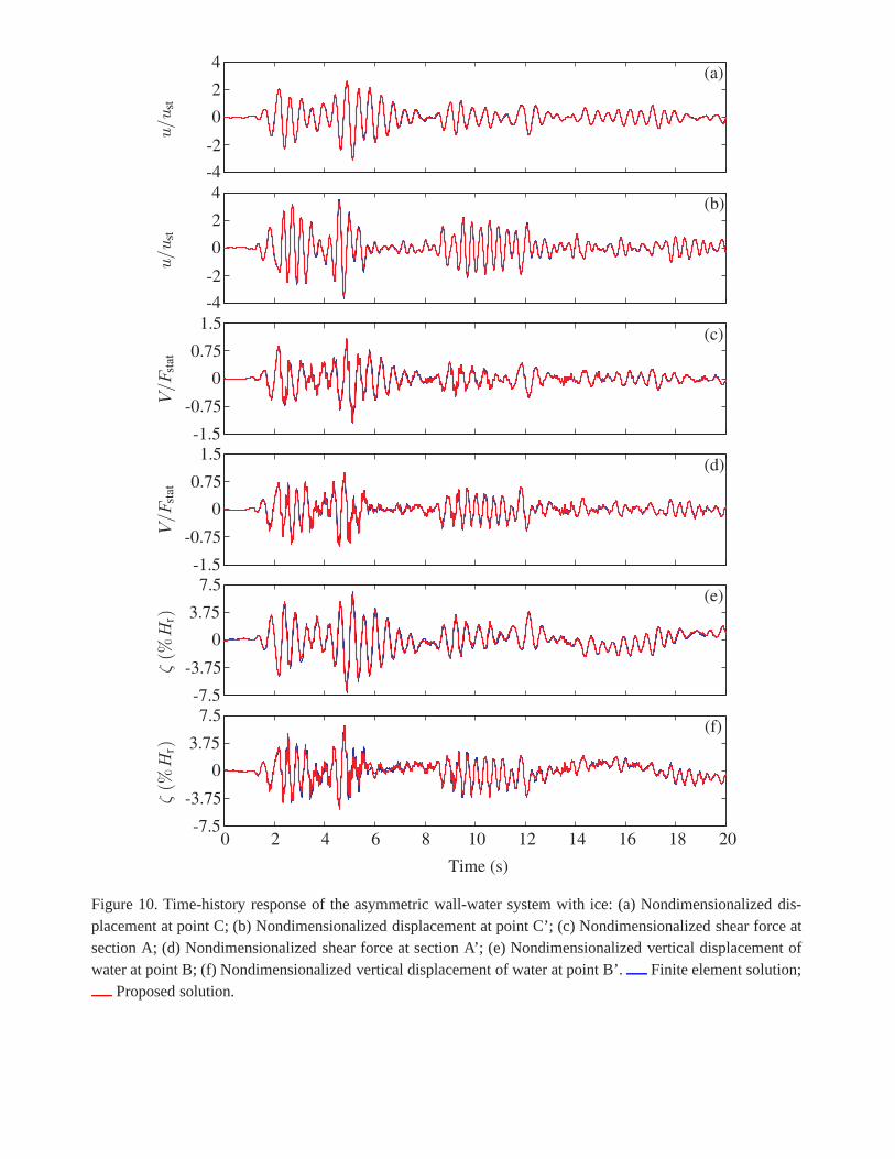
Figure 10. Time-history response of the asymmetric wall-water system with ice: (a) Nondimensionalized dis-placement at point C; (b) Nondimensionalized displacementat point C’; (c) Nondimensionalized shear force atsection A; (d) Nondimensionalized shear force at section A’; (e) Nondimensionalized vertical displacement ofwater at point B; (f) Nondimensionalized vertical displacement of water at point B’. Finite element solution;
Proposed solution.
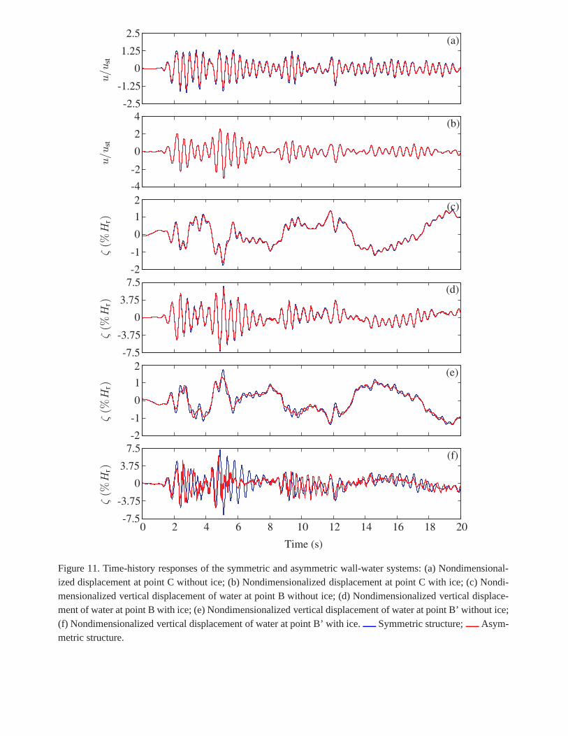
Figure 11. Time-history responses of the symmetric and asymmetric wall-water systems: (a) Nondimensional-ized displacement at point C without ice; (b) Nondimensionalized displacement at point C with ice; (c) Nondi-mensionalized vertical displacement of water at point B without ice; (d) Nondimensionalized vertical displace-ment of water at point B with ice; (e) Nondimensionalized vertical displacement of water at point B’ without ice;(f) Nondimensionalized vertical displacement of water at point B’ with ice. Symmetric structure; Asym-metric structure.


![ACI-350[1].3-06 Seismic Design of Liquid-Containing](https://img.pdfslide.net/doc/110x75/55cf9793550346d033925fad/aci-35013-06-seismic-design-of-liquid-containing.jpg)