SEISMIC ATTRIBUTE ANALYSIS USING HIGHER ORDER …

SEISMIC ATTRIBUTE ANALYSIS USING HIGHER ORDER STATISTICS

A Thesis

by

JANELLE GREENIDGE

Submitted to the Office of Graduate Studies of Texas A&M University

in partial fulfillment of the requirements for the degree of

MASTER OF SCIENCE

August 2008

Major Subject: Geophysics

SEISMIC ATTRIBUTE ANALYSIS USING HIGHER ORDER STATISTICS

A Thesis

by

JANELLE GREENIDGE

Submitted to the Office of Graduate Studies of Texas A&M University

in partial fulfillment of the requirements for the degree of

MASTER OF SCIENCE

Approved by:

Chair of Committee, Luc T. Ikelle Committee Members, John R. Hopper Daulat D. Mamora Head of Department, Andreas K. Kronenberg

August 2008

Major Subject: Geophysics

iii

ABSTRACT

Seismic Attribute Analysis Using Higher Order Statistics. (August 2008)

Janelle Greenidge, B.S., University of the West Indies

Chair of Advisory Committee: Dr. Luc T. Ikelle

Seismic data processing depends on mathematical and statistical tools such as

convolution, crosscorrelation and stack that employ second-order statistics (SOS).

Seismic signals are non-Gaussian and therefore contain information beyond SOS. One of

the modern challenges of seismic data processing is reformulating algorithms e.g.

migration, to utilize the extra higher order statistics (HOS) information in seismic data.

The migration algorithm has two key components: the moveout correction, which

corresponds to the crosscorrelation of the migration operator with the data at zero lag

and the stack of the moveout-corrected data. This study reformulated the standard

migration algorithm to handle the HOS information by improving the stack component,

having assumed that the moveout correction is accurate. The reformulated migration

algorithm outputs not only the standard form of stack, but also the variance, skewness

and kurtosis of moveout-corrected data.

The mean (stack) of the moveout-corrected data in this new concept is equivalent

to the migration currently performed in industry. The variance of moveout-corrected

data is one of the new outputs obtained from the reformulation. Though it characterizes

SOS information, it is not one of the outputs of standard migration. In cases where the

seismic amplitude variation with offset (AVO) response is linear, a single algorithm that

iv

outputs mean (stack) and variance combines both the standard AVO analysis and

migration, thereby significantly improving the cost of seismic data processing.

Furthermore, this single algorithm improves the resolution of seismic imaging, since it

does not require an explicit knowledge of reflection angles to retrieve AVO information.

In the reformulation, HOS information is captured by the skewness and kurtosis

of moveout-corrected data. These two outputs characterize nonlinear AVO response and

non-Gaussian noise (symmetric and nonsymmetric) that may be contained in the data.

Skewness characterizes nonsymmetric, non-Gaussian noise, whereas kurtosis

characterizes symmetric, non-Gaussian noise. These outputs also characterize any errors

associated with moveout corrections.

While classical seismic data processing provides a single output, HOS-related

processing outputs three extra parameters i.e. the variance, skewness, and kurtosis.

These parameters can better characterize geological formations and improve the

accuracy of the seismic data processing performed before the application of the

reformulated migration algorithm.

v

DEDICATION

To my beloved mom and dad, for your love, wisdom and support

vi

ACKNOWLEDGEMENTS

I would like to take this opportunity to give my sincere thanks to my academic

advisor and the Chair of my Graduate Committee, Dr. Luc Ikelle, for his teaching and

support throughout my research. His availability and timely guidance were fundamental

to the completion of my program. I am extremely grateful to my other Graduate

Committee members, Dr. John Hopper and Dr. Daulat Mamora, for their advice,

insightful comments and willingness to share their valuable time during my research

period.

My appreciation also goes out to the sponsors of the CASP project, whose

resources have made this and other research possible, and to fellow CASP members for

their assistance, suggestions and technical support.

Thanks also to the Government of Trinidad and Tobago for rewarding me a

scholarship to pursue this degree. Their funding and support during my time at Texas

A&M were greatly appreciated.

I wish to extend my gratitude to my family and friends for their unconditional

love, patience and support throughout my graduate studies at Texas A&M. Their

devotion has been very instrumental in my ability to complete this thesis successfully.

Most importantly, I give my thanks to God, with whom all things are possible.

vii

TABLE OF CONTENTS

Page

ABSTRACT……………………………………………………………………… iii

DEDICATION…………………………………………………………………… v

ACKNOWLEDGEMENTS……………………………………………………… vi

TABLE OF CONTENTS………………………………………………………… vii

LIST OF TABLES……………………………………………………………….. ix

LIST OF FIGURES…………………………………………………………….… x

CHAPTER

I INTRODUCTION…………………………………………………… 1

II SOME BACKGROUND OF STATISTICAL AVERAGES OF

NON-GAUSSIAN RANDOM VARIABLES……..………………... 13

Introduction………………………………………………………. 13 Moments and Cumulants…………………………………………. 14 Non-Gaussian Probability Distribution…………………………... 16

III HOS AND AVO SEISMIC DATA…………………………………. 19

Introduction………………………………………………………. 19 Examples of the Effect of Noise on CMP AVA Seismic Data…… 21 Analysis of Results……………………………………………….. 21

IV ANALYSIS OF HOS MIGRATION THROUGH

ONE-DIMENSIONAL GEOLOGICAL MODELS………………… 34

Formulation of the HOS Migration Algorithm…………………… 34 Description of Model……………………………………………... 35

Examples of HOS Migration……………………………………... 38 Analysis of Results……………………………………………….. 38

V SUMMARY AND CONCLUSIONS……………………………….. 44

viii

Page

REFERENCES……………………………………………………………………. 46

APPENDIX A…………………………………………………………………….. 47

VITA…………………………………………………………………………… .… 52

ix

LIST OF TABLES

TABLE Page

2.1 First four orders of cumulants…………………………………………… 15

2.2 Relation between the first five orders of moments and cumulants……… 16

2.3 First four moments and cumulants of the Gaussian, Laplace, Uniform

and Rayleigh distributions………………………………………………. 18

3.1 Statistical averages of AVO seismic data for different types and

variances of additive noise presented in Figures 3.2 to 3.9…..……….… 30

4.1 Output parameters of HOS migration…………………………………… 35

4.2 Parameters defining the geological model used for analysis of the new

HOS migration algorithm……………………………………………….. 37

x

LIST OF FIGURES FIGURE Page

1.1 Three key steps in seismic imaging……………………………………… 1

1.2 An illustration of the ray paths of seismic events in marine data…..….… 2

1.3 Typical ray path of primaries in the context of migration techniques as

used in this thesis…………………………………………………………. 4

1.4 An example of the process of migration……………….………………… 7

1.5 An example of the process of migration……………….………………… 8

1.6 An example of the process of migration using an incorrect moveout

velocity………………………………………………….……………..… 10

2.1 An illustration of a CMP gather before and after NMO correction……… 13

3.1 Typical ray paths of seismic energy in a model comprising two

homogeneous half-spaces………………………………………………... 19

3.2 Effect of Gaussian noise on linear AVA seismic data for different

variances of the noise…………………………………………………….. 22

3.3 Effect of Gaussian noise on nonlinear AVA seismic data for different


3.4 Effect of Laplacian noise on linear AVA seismic data for different


3.5 Effect of Laplacian noise on nonlinear AVA seismic data for different


xi

FIGURE Page

3.6 Effect of Rayleigh noise on linear AVA seismic data for different


3.7 Effect of Rayleigh noise on nonlinear AVA seismic data for different


3.8 Effect of Uniform noise on linear AVA seismic data for different


3.9 Effect of Uniform noise on nonlinear AVA seismic data for different


4.1 AVO Classification based upon reflection coefficient and offset

(Barton and Crider, 1999)………………………………………………... 36

4.2 AVO moveout-corrected seismic data of geological model……………... 38

4.3 AVO moveout-corrected seismic data used for example 1 and the

corresponding statistical averages………………………….…………….. 40





1

CHAPTER I

INTRODUCTION

The three key steps involved in seismic imaging are multiple-attenuation,

velocity-analysis, and migration with or without AVO (amplitude variations with

offsets), depending on exploration and production objectives. The three steps are

performed in the order assigned in Figure 1.1, i.e., demultiple and deghosting followed

by velocity estimation followed by migration with or without AVO-A. Let us start by

reviewing these three steps.

FIGURE 1.1 Three key steps in seismic imaging. The first steps are demultiple and deghosting and

velocity estimation. When followed by migration we obtain the structural image of the subsurface; the

interpretation in this case is characterized as structural. When followed by migration with AVO-A we

obtain more than the structure of the subsurface. We can also obtain the physical properties of the rock

formation; the interpretation in this case is characterized as quantitative.

_______________ This thesis follows the style and format of Geophysics.

Demultiple and Deghosting

Velocity Estimation

Migration AVO-A + Migration

Stru

ctur

al I

nter

pret

atio

n

Quantitative Interpretation

2

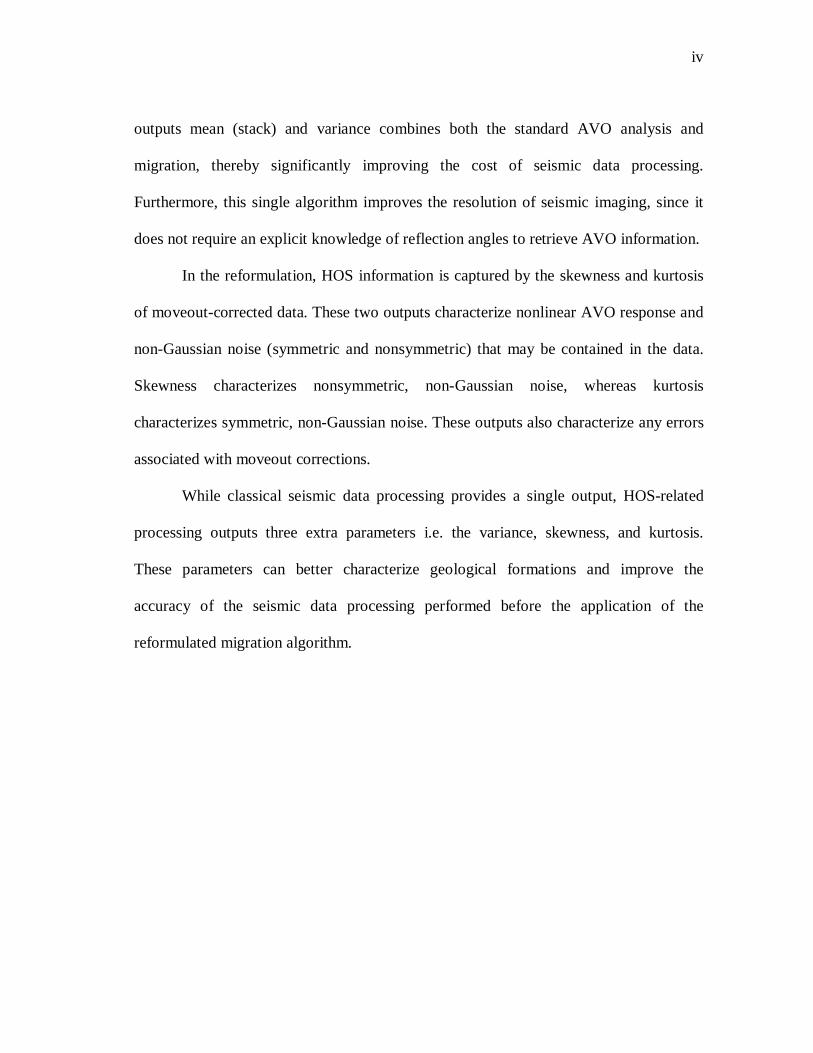
FIGURE 1.2 An illustration of the ray paths of seismic events in marine data.

1st order free-surface 2nd order free-surface

sea floor

source

receiver

free surface

source

receiver

free surface

sea

PRIMARIES

free surface

sea floor

sourc

receiver INTERNAL MULTIPLES

FREE-SURFACE MULTIPLES

3

Seismic data, especially those related to marine acquisition geometries, on which

the examples of this thesis are based, contain free-surface multiples, internal multiples

and primaries. Figure 1.2 illustrates typical ray paths describing the seismic events in

marine data. Note that the common seismic conventions have been used by not taking

into account Snell’s laws when drawing the ray paths. However, all computations follow

Snell’s laws.

The goal of the demultiple and deghosting step in seismic imaging is to produce

data that are void of multiples and ghosts. In the last two decades, significant efforts

have been made to address the multiple-attenuation problem. For example, Watts (2005)

and Singh (2005) have presented very efficient algorithms for removing free-surface

multiples and demonstrated the feasibility of the technologies in very complex

geologies. In this thesis, data containing only primaries will be considered. In other

words, it has assumed that multiples have been removed from the data.

We will now consider velocity estimation and the migration of seismic data with

only primaries. The velocity estimation and migration steps in seismic imaging are

intertwined. Although the velocity model must be estimated before performing migration

as described in Figure 1.2, the migration algorithm needs to be formulated first because

velocity-estimation is based on the same algorithm as migration.

Let us denote xs, the source position, xr, the receiver position and x, the image

point, as depicted in Figure 1.3.

4

interface

FIGURE 1.3 Typical ray path of primaries in the context of migration techniques as used in this thesis.

A field of primaries can be described in the frequency-space (F-X) domain, as

follows:

P(xs, xr, ω) = ∫ ω) ,( xx ,G s M(x) G(x, xr, ω) dx, (1.1)

where P(xs, xr, ω) is the field of primaries, G (xs, x, ω) is the Green’s function which

describes wave propagation from source to image point, G (x, xr, ω) is the Green’s

function which describes wave propagation from image point to receiver, and M(x)

characterizes the physical properties of the subsurface. It must be emphasized here that

the model used in equation (1.1) to describe our data is only valid for primaries, and

hence the assumption that multiples (free-surface multiples and internal multiples) have

been attenuated is needed.

Equation (1.1) can also be written as follows:

P(xs, xr, ω) =∫ ω) , , ,L( rs xxx M(x) dx, (1.2)

xs xr

x

source

receiver

image point

5

where L(xs, x, xr, ω) = G(xs, x, ω) G(x, xr, ω). The operator L is generally known as the

migration operator. One can seek to solve for M(x) through a classical inverse-problem

technique such as the least-square-optimization technique. However, if we assume that

the data have been corrected for geometrical spreading, the inverse solutions of equation

(1.2) can be expressed as follows (Ikelle and Amusden, 2005):

M(x) ≈ ∫∫∫ dωdd rs xx L*(xs, x, xr, ω) P(xs, xr, ω), (1.3)

where L* is the complex conjugate of L. The approximate solution M(x) is known as

migration. Notice that the solution in equation (1.3) can be rewritten as follows:

M(x) = ∫∫ rs dd xx M'(xs, x, xr), (1.4)

where M'(xs, x, xr) = ∫dω L*(xs, x, xr, ω) P(xs, xr, ω). This formula depicts the two

critical steps involved in migration. The first step involves the computation of M'(xs, x,

xr), which corresponds to the moveout correction of data. Notice that this computation is

equivalent to taking the crosscorrelation of the migration operator L and the data at zero

lag. Therefore the operator L must be very similar to the data to produce effective

moveout-corrected data. The second step, which corresponds to reconstructing M(x), is

equivalent to summing M' over the source and receiver positions. This is known as stack.

To develop more insight into the migration formula (1.4), let us look at the

particular case of a 1D model of the earth. In this case, the data P(xs, xr, ω) depends only

on offset, i.e.

P(xs, xr, ω) = P(xs-xr, 0, ω) = P1D(xs-xr, ω) = P1D(xh, ω) (1.5)

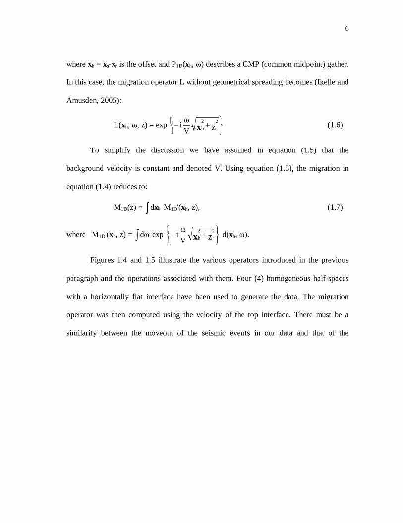
6

where xh = xs-xr is the offset and P1D(xh, ω) describes a CMP (common midpoint) gather.

In this case, the migration operator L without geometrical spreading becomes (Ikelle and

Amusden, 2005):

L(xh, ω, z) = exp

+− z22

hV

ωi x (1.6)

To simplify the discussion we have assumed in equation (1.5) that the

background velocity is constant and denoted V. Using equation (1.5), the migration in

equation (1.4) reduces to:

M1D(z) = ∫ hdx M1D'(xh, z), (1.7)

where M1D'(xh, z) = ∫dω exp

+− z22

hV

ωi x d(xh, ω).

Figures 1.4 and 1.5 illustrate the various operators introduced in the previous

paragraph and the operations associated with them. Four (4) homogeneous half-spaces

with a horizontally flat interface have been used to generate the data. The migration

operator was then computed using the velocity of the top interface. There must be a

similarity between the moveout of the seismic events in our data and that of the

7

FIGURE 1.4 An example of the process of migration. (a) CMP gather, P1D. (b) Moveout-corrected gather, M1D', produced using the

appropriate moveout velocity. (c) Stack of moveout-corrected data, M1D.

Example 1

Time (s) Time (s) Time (s)

Offset (km) Offset (km)

0

2

1

0 2 4 -2 -4 x 10-5

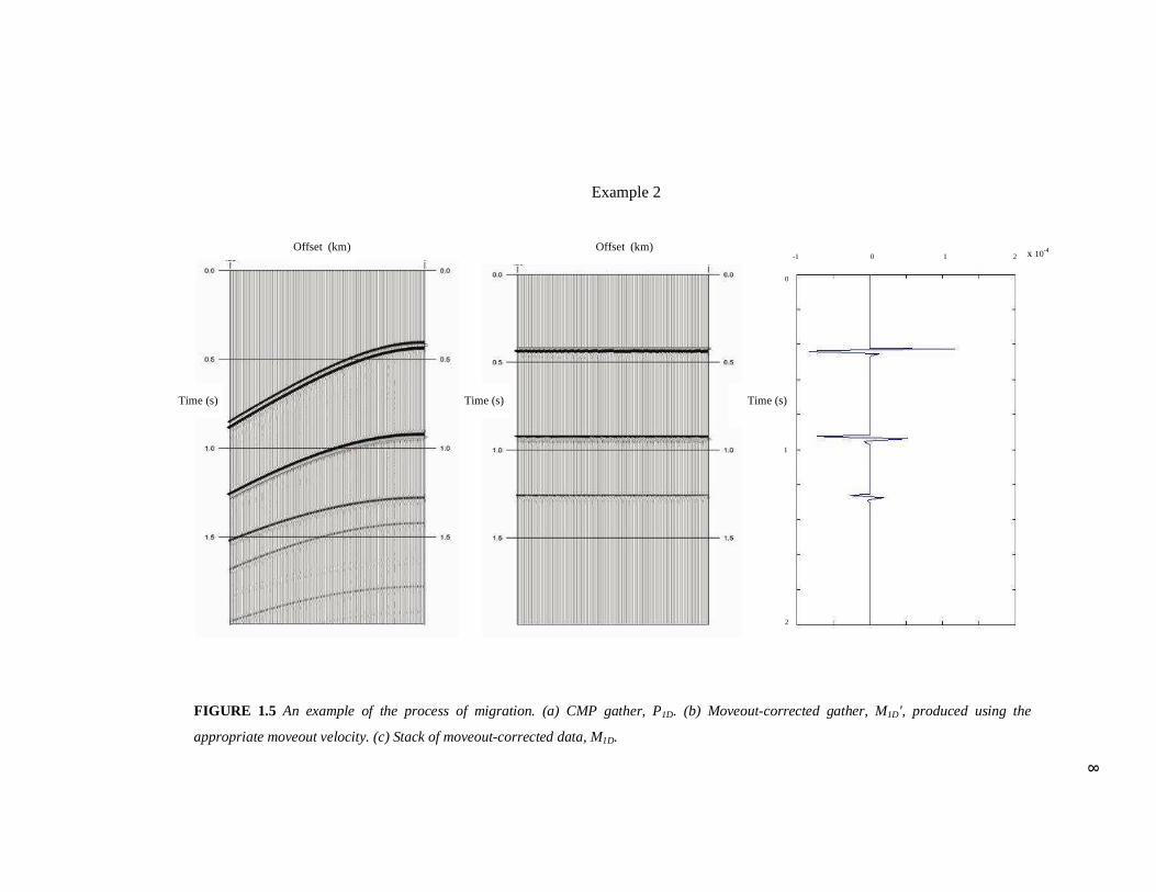
8

FIGURE 1.5 An example of the process of migration. (a) CMP gather, P1D. (b) Moveout-corrected gather, M1D', produced using the

appropriate moveout velocity. (c) Stack of moveout-corrected data, M1D.

Example 2

Time (s) Time (s) Time (s)


0

1

2

0 1 2 -1 x 10-4

9

migration operator. The moveout-corrected data, M1D'(xh, z), which corresponds to the

crosscorrelation of L(xh, ω, x) and P1D(xh, ω) at zero lag, is obviously flat as can be seen

in Figures 1.4 and 1.5. Normally, the AVO analysis, which will be discussed later, is

taking place on the moveout-corrected data, M1D'(xh, z) in Figures 1.4 (c) and 1.5 (c),

with each offset converted into reflection angle. The migration is then performed to

obtain M1D(z) which allows us to locate the reflector.

Now that we have introduced the migration techniques, let us describe the second

step of the processing chain, as depicted in Figure 1.1, i.e. velocity-analysis. As can be

seen from the examples in Figures 1.4 and 1.5, the moveout-corrected data is very

sensitive to the shape of the migration operator, which in turn is very sensitive to the

velocity model. In Figure 1.6 the moveout-corrected migration operator is different from

that of the moveout-corrected data. Therefore, M1D'(xh, z) in this case is no longer flat.

So the basic idea of velocity-analysis consists of computing M1D'(xh, z) for various

velocity models and selecting the one for which the moveout-corrected data are flat. In

this thesis, we will assume that the velocity-analysis has been performed and therefore

we assume that we have a correct velocity model.

Assuming that we now have a correct velocity model, M'(xs, x, xr) can now be

constructed, and from M'(xs, x, xr) migrated sections M(x) can be produced, as described

in equation (1.3). However, such an image will provide the locations of key reflectors in

the subsurface without providing any information about the change of properties that

cause the reflections. An alternative approach is to use the moveout-corrected data,

10

FIGURE 1.6 An example of process of migration using an incorrect moveout velocity. (a) CMP gather, P1D. (b) Moveout-corrected gather, M1D',

produced using an inappropriate moveout velocity. (c) Stack of moveout- corrected data, M1D.

Time (s) Time (s)

Time (s)

0

1

2


x 10-5 -1 0 1 2

11

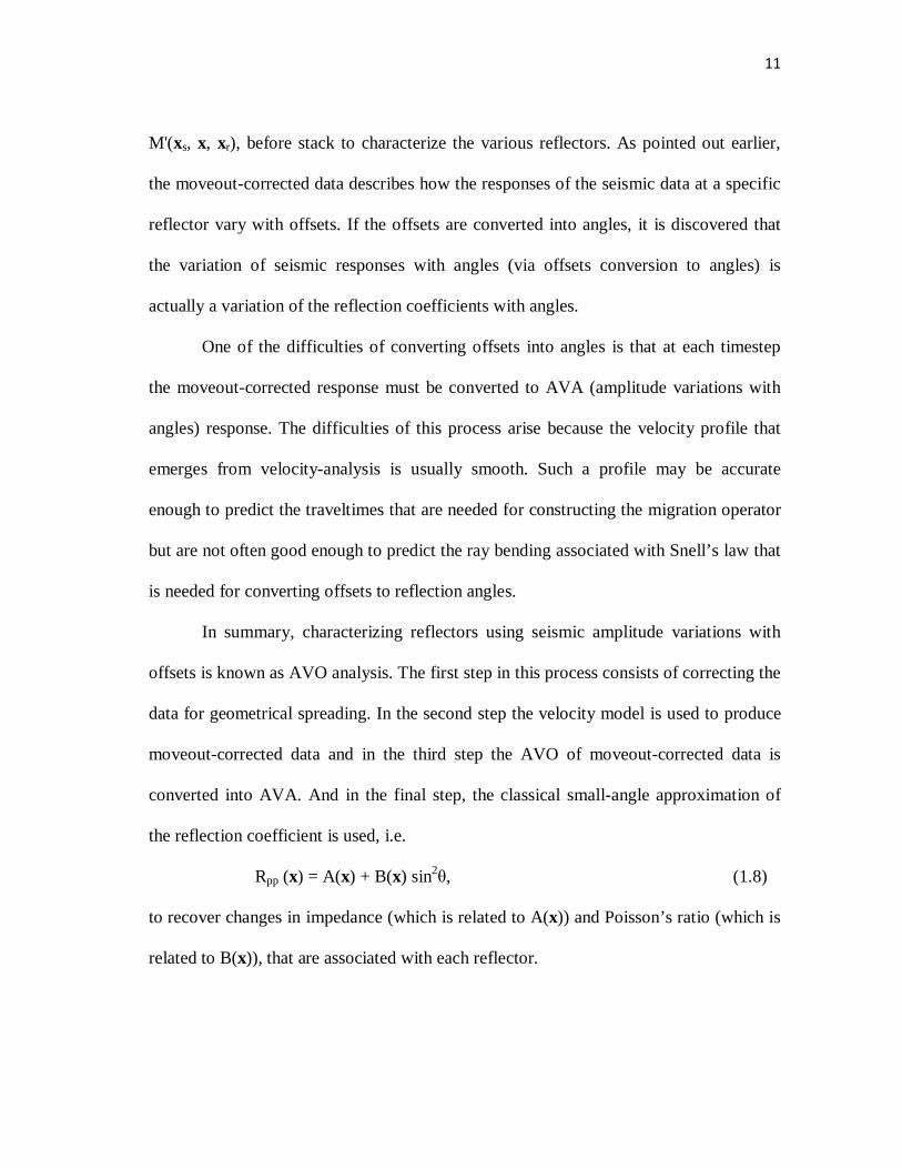
M'(xs, x, xr), before stack to characterize the various reflectors. As pointed out earlier,

the moveout-corrected data describes how the responses of the seismic data at a specific

reflector vary with offsets. If the offsets are converted into angles, it is discovered that

the variation of seismic responses with angles (via offsets conversion to angles) is

actually a variation of the reflection coefficients with angles.

One of the difficulties of converting offsets into angles is that at each timestep

the moveout-corrected response must be converted to AVA (amplitude variations with

angles) response. The difficulties of this process arise because the velocity profile that

emerges from velocity-analysis is usually smooth. Such a profile may be accurate

enough to predict the traveltimes that are needed for constructing the migration operator

but are not often good enough to predict the ray bending associated with Snell’s law that

is needed for converting offsets to reflection angles.

In summary, characterizing reflectors using seismic amplitude variations with

offsets is known as AVO analysis. The first step in this process consists of correcting the

data for geometrical spreading. In the second step the velocity model is used to produce

moveout-corrected data and in the third step the AVO of moveout-corrected data is

converted into AVA. And in the final step, the classical small-angle approximation of

the reflection coefficient is used, i.e.

Rpp (x) = A(x) + B(x) sin2θ, (1.8)

to recover changes in impedance (which is related to A(x)) and Poisson’s ratio (which is

related to B(x)), that are associated with each reflector.

12

The stack of moveout-corrected data, i.e., M'(xs, x, xr) in equation (1.4) and

M1D'(xh, z) in equation (1.7), is actually equivalent to taking the mean of these data at

each timestep. In this thesis, we propose to compute the variance of the same moveout-

corrected data at each timestep. It turns out that outputting both the mean and variance is

equivalent to recovering the AVO parameters, A(x) and B(x), without the complex step

of converting AVO to AVA. Moreover, the computation of mean and variance can be

done in parallel, hence eliminating most of the operations described above. As such, the

cost of seismic processing will be significantly reduced, as well as its accuracy, because

errors associated with converting offsets to angles will be avoided.

Because seismic events are non-Gaussian, as will be seen in Chapter II, we can

also output other cumulants such as skewness and kurtosis. In Chapter II, these

cumulants will be described, in addition to recalling the notion of non-Gaussianity and

the statistical concepts associated with it. We will demonstrate that outputting these

additional cumulants will allow us to characterize rock formations beyond the small-

angle approximation. In other words, we are also able to include nonlinear AVO. In

Chapter III, preliminary results will be provided that confirm the potential usefulness of

these new parameters for characterizing interfaces by discussing one dimensional (1-D)

examples.

13

CHAPTER II

SOME BACKGROUND OF STATISTICAL AVERAGES OF NON-GAUSSIAN

RANDOM VARIABLES

Introduction

Let us consider migrated data without stack. Each image/reflection point is

illuminated several times as illustrated in Fig 2.1 for 1D medium, as adapted from Ikelle

and Amundsen (2005).

FIGURE 2.1 An illustration of a CMP gather before and after NMO correction. The angle θ is the

incident angle.

The image point being imaged consists of N traces that correspond to N source-receiver

pairs or offsets. These traces are known as a common midpoint (CMP) gather. If an

NMO or traveltime correction is performed then for all offsets the traveltime from

Receiver position before NMO correction

Receiver position after NMO correction

Source position before NMO correction Source position after NMO correction

14

source to image point will be identical to the traveltime from image point to receiver.

Each offset can now be considered as descriptive of a random event and the set of events

as a random variable. Therefore, for each timestep, we can compute the statistical

averages.

The classical approach consists of summing the data to produce an image of that

point. However, since it is well recognized that the various illuminations contain more

information than the classical stack, geophysicists have developed several tools of

attribute analysis in order to extract this information. In this thesis, I propose an

alternative way of capturing this information. This new statistically based approach

consists of treating migrated data without stack as random variables. Hence, the

migrated data can be characterized at a given image point by either the statistical

moments or cumulants. In Chapters III and IV we will show the applications of this

concept.

This chapter focuses on a review of statistical averages, including the averages

associated with non-Gaussian random variables, and also on other basic statistical

notions that will be needed later on in this analysis.

Moments and Cumulants

Let us denote M (X, θ) as a random variable at point X. This random variable

varies with θ, the reflection angle. The statistical moments of this random variable can

be defined as follows:

mn (X, θ) = E[Mn] = dxxpxn )(∫∞

∞− (2.1)

15

where E is the mathematical expectation. For the particular case of the discrete random

variable, this can now be defined as:

mn (X, θ) = dxxpx kn )(∫

∞

∞− (2.2)

When n=1 we have the 1st order moment known as the mean, when n=2 we have

the 2nd order moment, etc. The migration defined so far in industry corresponds to the 1st

order moment (mean) only, and ignores the higher order statistics of the seismic data.

Therefore, if we stop here we would lose all the information about the other moments,

especially those related to non-Gaussianity.

An alternative way to describe non-Gaussian random variables is to introduce the

cumulant. The first four orders are defined in the Table 2.1 below.

TABLE 2.1 First four orders of cumulants.

n Order

Cumulants

(cn) Statistical Name

1 1st c1 Mean

2 2nd c2 Variance

3 3rd c3 Skewness

4 4th c4 Kurtosis

Using X as a random variable, the relation between cumulants and moments has

been described in Table 2.2 below, as adapted from Ikelle and Amundsen (2005). The

quantity c1 (or m1) is the mean, c2 (or µ2) is the variance, c3 is the skewness and c4 is the

kurtosis.

16

TABLE 2.2 Relation between the first five moments and cumulants.

n Moments

(mn) Central Moments

(µµµµn) Cumulants

(cn)

Cumulants(cn) for zero mean

random variable

0 mo = 1 µ0 = 1 c0 = 0 c0 = 0

1 m1 = E(x) µ1 = 0 c1 = m1 c1 = 0

2 m2 = E(x2) µ2 = m2 – m12 c2 = m2 – m1

2 c2 = m2

3 m3 = E(x3) µ3 = m3 – 3 m2m1 + 2 m13 c3 = m3 – 3 m2m1 + 2 m1

3 c3 = m3

4 m4 = E(x4) µ4 = m4 – 4 m3m1 + 6 m2 m12 – 3m1

4 c4 = m4 – 4 m3m1 – 3 m22 + 12 m2 m1

2 – 6m14 c4 = m4 – 3 m2

2

For more information on random variables, moments and cumulants see Appendix A.

Non-Gaussian Probability Distributions

The first 2 orders of moments and cumulants (i.e. the mean and variance) are

characterized as Gaussian or second order statistics (SOS), and moments and cumulants

greater than the second order (e.g. skewness and kurtosis) are characterized as higher

order statistics (HOS). When the HOS cumulants are zero they are also characterized as

Gaussian, however once the cumulants of order greater than two have non-null values

they are characterized as non-Gaussian.

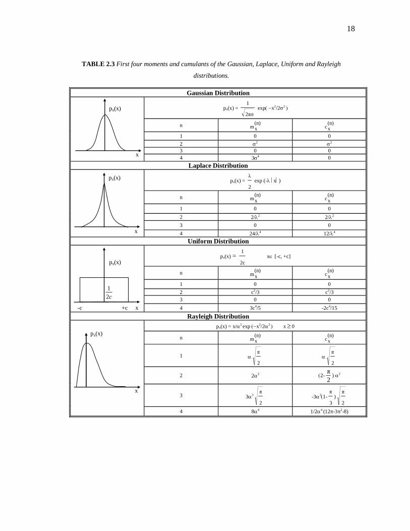
Table 2.3 provides detailed descriptions about the moments and cumulants for

different probability density functions. It effectively confirms that for non-Gaussian

random variables, the higher order cumulants are non-zero. Notice also that for

symmetric distributions the odd cumulants, e.g. the 3rd order cumulant (skewness), are

zero. This can clearly be observed with the Laplace and Uniform distributions, chosen

because they describe the extreme cases; the Uniform distribution with negative kurtosis

(sub Gaussian) and the Laplace distribution with positive kurtosis (super Gaussian).

17

In Table 2.3, the Rayleigh distribution shows an example of non-Gaussian, non-

symmetric random variables. We can see that when the random variable is non-Gaussian

and non-symmetric that we have extra information through both the skewness and

kurtosis.

To date, the extra information that can be captured in the HOS has not yet been

exploited in seismic data processing. Practical seismic data processing is actually limited

to the mean, since the variance is not really used. Techniques based on SOS recover only

limited information about non-Gaussian signals, and as such information related to

deviations from Gaussianity is not extracted. Better results can be realized using HOS

over SOS, since HOS allows for the processing of seismic signals that are non-Gaussian.

Studying the higher order statistics will allow information extra to that used in traditional

seismic imaging to be utilized. This will enable better estimates of parameters in noisy

situations or shed light on non-linearities that may be inherent in the seismic data.

One of challenges that will be addressed in the next chapter is not only recovery

of the seismic attributes: the mean, variance, skewness and kurtosis for each image

point, but also connecting this new information to specific geologies. For example, in

areas where the reflection coefficient can be described by R = A + B x, the skewness and

kurtosis are expected to be zero. Here A will basically characterize the mean and B can

characterize the variance. In other words, the statistical averages can be used to recover

A or B at small angles. As more realistic cases are considered, HOS can then be utilized

to characterize the other parameters.

18

TABLE 2.3 First four moments and cumulants of the Gaussian, Laplace, Uniform and Rayleigh

distributions.

px(x)

x

px(x)

x

px(x)

-c

px(x)

x

+c x

Gaussian Distribution

px(x) = σ2π

1 exp( −x2/2σ2 )

n (n)xm

(n)xc

1 0 0

2 σ2 σ2 3 0 0 4 3σ4 0

Laplace Distribution

px(x) = 2

λ

exp (-λ x)

n (n)xm

(n)xc

1 0 0

2 2/λ2 2/λ2

3 0 0

4 24/λ4 12/λ4

Uniform Distribution

px(x) = 2c

1 x∈ [-c, +c]

n (n)xm (n)

xc 1 0 0

2 c2/3 c2/3 3 0 0

4 3c4/5 -2c4/15

Rayleigh Distribution px(x) = x/α2 exp (−x2/2α2 ) x≥ 0

n (n)xm (n)

xc

1 α2

π

α2

π

2 2α2 (2-2π

) α2

3 3α3

2

π

-3α3(1-3

π

)2

π

4 8α4 1/2α4 (12π-3π2-8)

c2

1

19

CHAPTER III

HOS AND AVO SEISMIC DATA

Introduction

Energy is partitioned into reflected and transmitted energy at an interface that

separates two different layers, as illustrated in Figure 3.1. The reflection and

transmission is dependent on the angle of incidence, θ of the incoming wave, as well as

the physical properties of the two layers. The seismic amplitudes of the reflected and

transmitted energy depend on the contrast in the physical properties across the boundary,

i.e. the amplitudes carry information about the contrast of elastic parameters of two (2)

rock formations. The Zoeppritz equations, which define the reflection and transmission

coefficients, are used to relate the reflected and transmitted energy to the physical

properties of the two layers. In this thesis, we will only refer to the reflection coefficient.

FIGURE 3.1 Typical ray paths of seismic energy in a model comprising two homogeneous half-spaces.

Transmitted wave

Incident wave

V1, ρ1

Reflected wave

V2, ρ2

θi θr

θt

θi = angle of incidence

θt = angle of transmission

θr = angle of reflection

V1 = velocity of wave in upper medium

V2 = velocity of wave in lower medium

ρ1 = density of upper medium

ρ2 = density of lower medium

20

The linearized expressions of the Zoeppritz equations are derived using the

small-angle approximation. For the reflection coefficient the linear approximation can be

given by:

R = A + B x (3.1)

where x = sin2θ

At larger angles, the reflection coefficient can be given by:

R = A + B x + C x2 (3.2)

This is a second order approximation in x. Numerically it has been shown that the linear

approximation works best for angles of θ < 35° and the second order approximation

works best for angles of θ < 60°, after which the expressions become unstable.

These approximations produce small inaccuracies and are incorporated in the

seismic data as noise. In practice, the noise associated with the seismic data acquisition

geometries is also integrated into the data. For this reason, the reflection coefficient

given in equation (3.2) above can now be described by:

R = A + B x + C x2 + η = Ro + η (3.3)

where Ro = A + B x + C x2

In this thesis we will describe Ro and η as two (2) random variables.

21

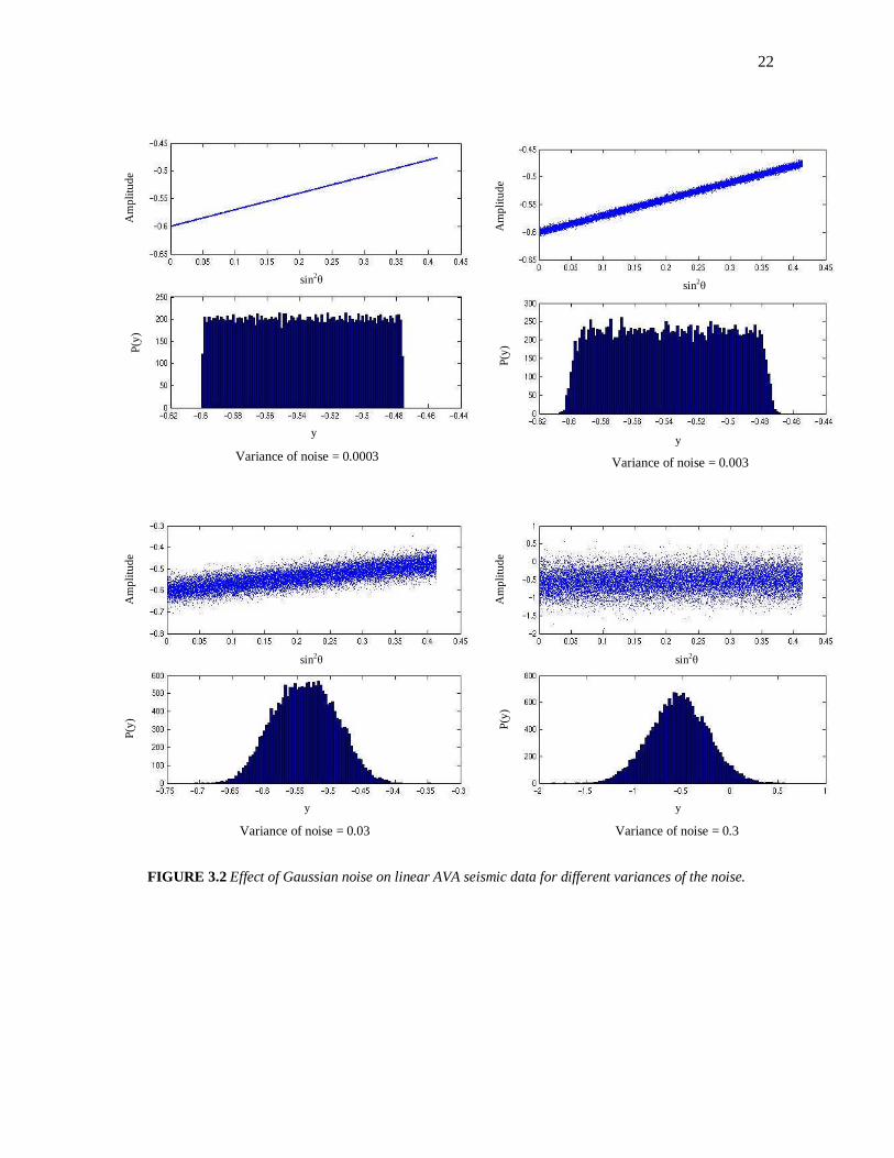
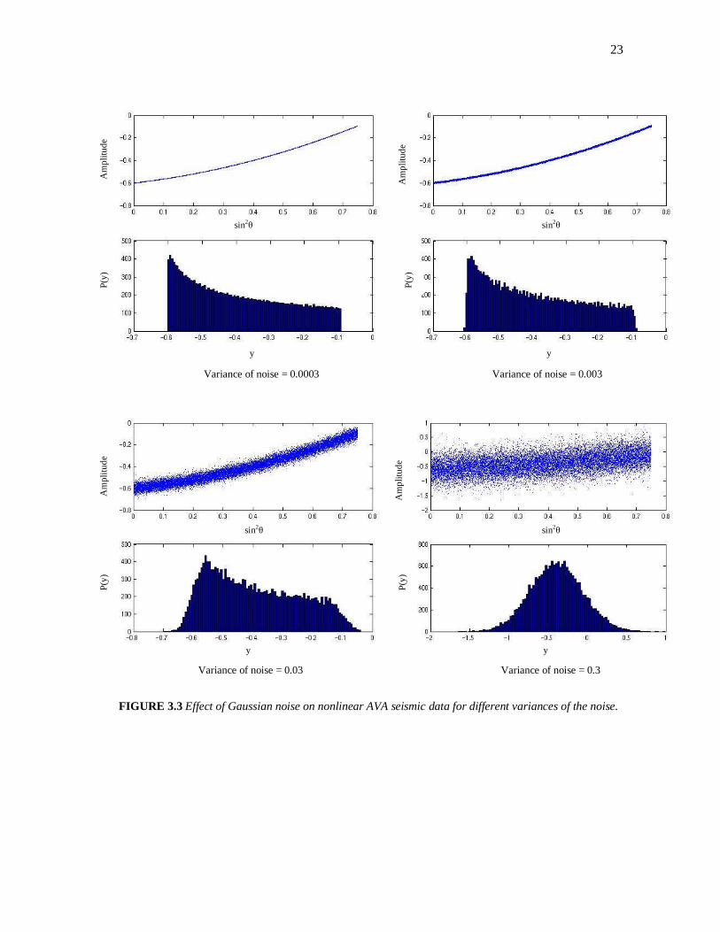
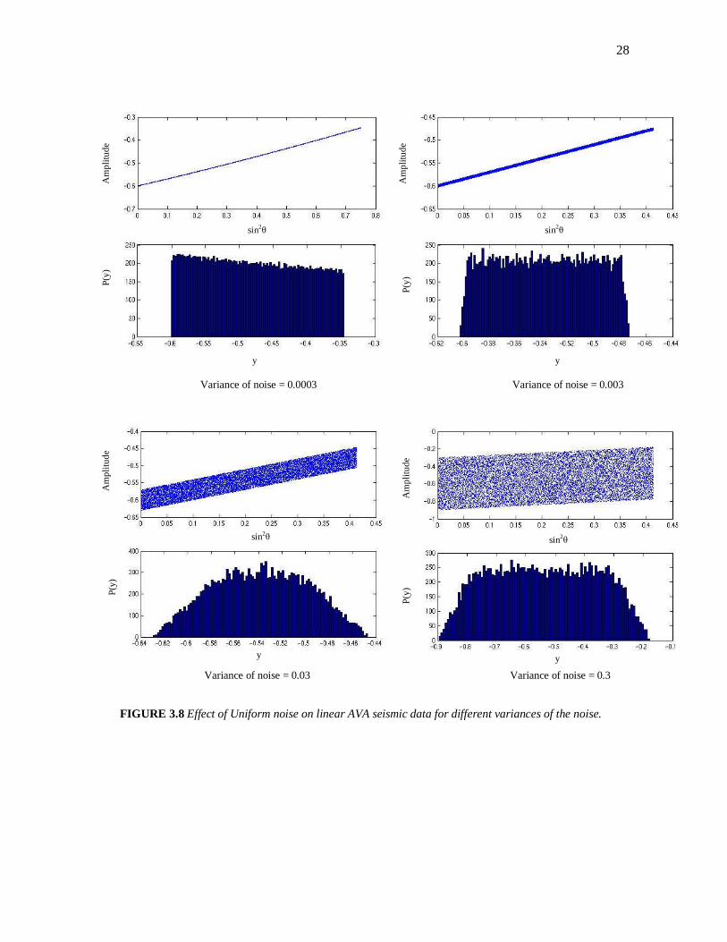
Examples of the Effect of Noise on CMP AVA Seismic Data

Consider several examples of CMP AVA data in Figures 3.2 to 3.9. These

examples show the effect of adding different types and variances of noise to linear and

nonlinear AVA. Each figure contains four (4) diagrams of the AVA data and their

associated histograms, as the variance of the noise added is increased. We have also

computed the corresponding statistical averages for these examples as illustrated in

Table 3.1.

Analysis of Results

From the histograms, we can observe that as the order of the noise is increased,

the data tends more and more toward the type of noise that is added. It is also clear that

seismic data does not tend to the Gaussian distribution. Therefore, we can characterize

seismic data at a given image point as non-Gaussian random variables. The experiment

was repeated several times giving the same conclusion that the seismic data behaved

more like a non-Gaussian distribution.

So one might ask the following question: In what cases can seismic data be

described by a Gaussian random variable? One possible case is that the seismic response

is invariant with the reflection angle. This is however non physical, since we can see

from the Zoeppritz equations that it is impossible to have constant reflection coefficient

with angle. Alternatively, we can get a Gaussian distribution if the reflection coefficients

22

FIGURE 3.2 Effect of Gaussian noise on linear AVA seismic data for different variances of the noise.

Variance of noise = 0.0003 Variance of noise = 0.003


sin2θ sin2

θ

sin2θ sin2

θ

Am

plit

ud

e

Am

plit

ud

e

Am

plit

ud

e

Am

plit

ud

e

P(y

) P

(y)

P(y

) P

(y)

y y

y y

23

FIGURE 3.3 Effect of Gaussian noise on nonlinear AVA seismic data for different variances of the noise.



sin2θ sin2

θ

sin2θ sin2

θ

Am

plit

ud

e

Am

plit

ud

e

Am

plit

ud

e

Am

plit

ud

e

P(y

) P

(y)

P(y

) P

(y)

y

y y

y

24

FIGURE 3.4 Effect of Laplacian noise on linear AVA seismic data for different variances of the noise.



sin2θ sin2

θ

sin2θ sin2

θ

Am

plit

ud

e

Am

plit

ud

e

Am

plit

ud

e

Am

plit

ud

e

P(y

) P

(y)

P(y

) P

(y)

y y

y y

25

FIGURE 3.5 Effect of Laplacian noise on nonlinear AVA seismic data for different variances of the noise.



sin2θ sin2

θ

sin2θ sin2

θ

Am

plit

ud

e

Am

plit

ud

e

Am

plit

ud

e

Am

plit

ud

e

P(y

) P

(y)

P(y

) P

(y)

y y

y y

26

FIGURE 3.6 Effect of Rayleigh noise on linear AVA seismic data for different variances of the noise.



sin2θ sin2

θ

sin2θ sin2

θ

Am

plit

ud

e

Am

plit

ud

e

Am

plit

ud

e

Am

plit

ud

e

P(y

) P

(y)

P(y

) P

(y)

y

y y

y

27

FIGURE 3.7 Effect Rayleigh noise on nonlinear AVA seismic data for different variances of the noise.



sin2θ

sin2θ sin2

θ

sin2θ

Am

plit

ud

e

Am

plit

ud

e

Am

plit

ud

e

Am

plit

ud

e

P(y

) P

(y)

P(y

) P

(y)

y

y y

y

28

FIGURE 3.8 Effect of Uniform noise on linear AVA seismic data for different variances of the noise.



sin2θ sin2

θ

sin2θ sin2

θ

Am

plit

ud

e

Am

plit

ud

e

Am

plit

ud

e

Am

plit

ud

e

P(y

) P

(y)

P(y

) P

(y)

y y

y y

29

FIGURE 3.9 Effect of Uniform noise on nonlinear AVA seismic data for different variances of the noise.



sin2θ sin2

θ

sin2θ sin2

θ

Am

plit

ud

e

Am

plit

ud

e

Am

plit

ud

e

Am

plit

ud

e

P(y

) P

(y)

P(y

) P

(y)

y

y

y

y

30

TABLE 3.1 Statistical averages of AVO seismic data for different types and variances of additive noise

presented in Figures 3.2 to 3.9.

Gaussian (Linear) Variance of Noise Mean Variance Skewness Kurtosis

0.0003 -0.538025 0.0012805 0.000172566 -0.0429237 0.003 -0.538022 0.00128765 0.000619463 -0.0424862 0.03 -0.538384 0.00218992 0.00316914 -0.0191433 0.3 -0.538449 0.0901212 0.0134413 0.00424079

Gaussian (Non-linear) Variance of Noise Mean Variance Skewness Kurtosis

0.0003 -0.393761 0.0217956 0.375146 -0.160141 0.003 -0.393801 0.0218062 0.375577 -0.159903 0.03 -0.393533 0.0226981 0.347874 -0.153352 0.3 -0.391978 0.111797 0.0458331 -0.00273106

LaPlacian (Linear) Variance of Noise Mean Variance Skewness Kurtosis

0.0003 -0.538027 0.00128005 1.90102e-05 -0.0429171 0.003 -0.538029 0.00129885 -0.00229077 -0.0420918 0.03 -0.537569 0.00311477 -0.012903 0.0590645 0.3 -0.536581 0.178466 0.0516943 1.27223

LaPlacian (Non-linear) Variance of Noise Mean Variance Skewness Kurtosis

0.0003 -0.393773 0.0217951 0.37518 -0.160133 0.003 -0.393801 0.0218226 0.374189 -0.160052 0.03 -0.393542 0.0235839 0.328764 -0.140445 0.3 -0.394912 0.201337 0.090346 1.09169

Rayleigh (Linear) Variance of Noise Mean Variance Skewness Kurtosis

0.0003 -0.537653 0.0012804 -3.13495e-05 -0.0429372 0.003 -0.534257 0.00128375 0.000470458 -0.0427205 0.03 -0.50051 0.00164901 0.0507358 -0.0277204 0.3 -0.160657 0.0404481 0.588773 0.0420479

Rayleigh (Non-linear) Variance of Noise Mean Variance Skewness Kurtosis

0.0003 -0.393385 0.0217955 0.375145 -0.160138 0.003 -0.389972 0.021791 0.374719 -0.160138 0.03 -0.35611 0.0222127 0.368259 -0.156131 0.3 -0.0173828 0.0605068 0.399546 -0.00997649

Uniform (Linear) Variance of Noise Mean Variance Skewness Kurtosis

0.0003 -0.538026 0.00128048 4.09828e-05 -0.042938 0.003 -0.538055 0.00128321 -0.000890827 -0.0427528 0.03 -0.538072 0.0015817 -0.00317656 -0.0329229 0.3 -0.538883 0.0311004 0.00700946 -0.193539

Uniform (Non-linear) Variance of Noise Mean Variance Skewness Kurtosis

0.0003 -0.393764 0.0217959 0.375178 -0.160142 0.003 -0.393768 0.0217955 0.375155 -0.160066 0.03 -0.393782 0.0220683 0.367511 -0.156631 0.3 -0.393237 0.0508386 0.106608 -0.128628

31

vary in the form, R = A + B sin2θ, where θ are uniformly distributed. Because seismic

data are sampled in offset, this scenario is also unrealistic. Thus, the random variables of

interest in this analysis are non-Gaussian most of the time.

Let us focus consider the histograms and statistics obtained for each example. In

all cases we can see that for very little variance of additive noise, the data is non-

Gaussian. The data is Uniform in the linear AVA case. As the variance of the noise is

increased to the point where there is too much noise, the data tend to the distribution of

the noise added.

For the case of the additive Gaussian noise with the linear AVA data, we see that

as the variance of the noise increases, the data tend toward a Gaussian distribution and

with the nonlinear AVA, the data tend toward a nonsymmetric non-Gaussian

distribution, i.e.

Linear AVO + Gaussian noise Gaussian data

Nonlinear AVO + Gaussian noise nonsymmetric, non-Gaussian data

There is a significant increase in the variance, skewness and kurtosis in the nonlinear

AVA case when compared to the linear AVA case. Again showing that despite the noise

being Gaussian, the data have been rendered non-Gaussian because of the nonlinear

AVA effect.

Consider the case of non-Gaussian noise with symmetric distributions, i.e.

Laplacian and Uniform noise. For additive Laplacian noise with the linear AVA data, we

see that as the variance of the noise increases, the data tend toward a symmetric, super

32

non-Gaussian distribution and with the nonlinear AVA, the data tend toward a

nonsymmetric non-Gaussian distribution, i.e.

Linear AVO + Laplacian noise symmetric, super non-Gaussian data

Nonlinear AVO + Laplacian noise nonsymmetric, non-Gaussian data

For additive Uniform noise with the linear AVA data, we see that as the variance of the

noise increases, the data tend toward a symmetric, sub non-Gaussian distribution and

with the nonlinear AVA, the data tend toward a nonsymmetric non-Gaussian

distribution, i.e.

Linear AVO + Uniform noise symmetric, sub non-Gaussian data

Nonlinear AVO + Uniform noise nonsymmetric, non-Gaussian data

For both types of additive noise, for the linear AVA case, the skewness is almost null for

all variances of noise, whereas in the nonlinear case the skewness is large and generally

constant for all variances of noise. The kurtosis in the linear AVA case though smaller is

significant and increases slightly, just as in the nonlinear case. For the Laplacian additive

noise, the kurtosis tends more to a positive value (super Gaussian), whereas for the

Uniform additive noise it tends to a more negative value (sub Gaussian). Hence, in order

to distinguish between Gaussian noise and non-Gaussian noise with symmetric

distributions, the kurtosis must be examined.

For the case of the non-Gaussian noise with nonsymmetric distributions, i.e.

Rayleigh noise, we see that with the both the linear and nonlinear AVA data, as the

variance of the noise increases, the data tend toward a nonsymmetric non-Gaussian

distribution.

33

Linear AVO + Rayleigh noise nonsymmetric, non-Gaussian data

Nonlinear AVO + Rayleigh noise nonsymmetric, non-Gaussian data

There is a significant increase in the skewness as the variance of the noise increases.

Similar to the Laplacian and Uniform noise, the kurtosis in the linear AVA case though

smaller is significant and increases slightly, just as in the nonlinear case.

Summarizing, we can say that the skewness can be used to characterize

nonsymmetric, non-Gaussian noise and the kurtosis can be used to characterize

symmetric, non-Gaussian noise in the data. Non-Gaussian data result from either the

presence of non-linear AVA effects or non-Gaussian noise. Also, since seismic data are

generally considered to be statistically symmetric, any significant value of skewness

may indicate bad processing and in this case it could be that the moveout correction was

not performed correctly.

34

CHAPTER IV

ANALYSIS OF HOS MIGRATION THROUGH ONE-DIMENSIONAL

GEOLOGICAL MODELS

The standard migration algorithm used in conventional seismic migration

consists of two major processes, moveout correction and then the stack of the moveout-

corrected data; as described earlier in Chapter I. Our formulation of this HOS migration

algorithm is based on adapting only the stack component of the standard algorithm.

Assuming that the moveout correction has been performed accurately, the stack

component is improved such that more information present in the seismic data can be

output from the new algorithm.

Formulation of the HOS Migration Algorithm

The formulation of the HOS migration algorithm is based on treating the

moveout-corrected data as a random variable, as discussed before. This moveout-

corrected data is defined by:

M'(xs, x, xr) = ∫dω L*(xs, x, xr, ω) P(xs, xr, ω) (4.1)

Traditional migration then sums this data over the receivers and sources to produce the

stack.

M(x) = ʃ dxs ʃ dxr M'(xs, x, xr) (4.2)

where P(xs, xr, ω) is the seismic data in the F-X domain and L(xs, x, xr, ω) is the

migration operator, as introduced in the previous chapter.

35

Instead of outputting only the stack, from the moveout-corrected data we can

output the parameters m1(x) to m4(x) as defined below:

m1(x) = ʃ dxs ʃ dxr M'(xs, x, xr), (4.3)

m2(x) = ʃ dxs ʃ dxr (M'(xs, x, xr))2, (4.4)



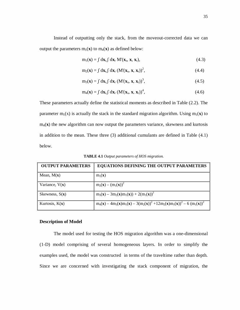
These parameters actually define the statistical moments as described in Table (2.2). The

parameter m1(x) is actually the stack in the standard migration algorithm. Using m1(x) to

m4(x) the new algorithm can now output the parameters variance, skewness and kurtosis

in addition to the mean. These three (3) additional cumulants are defined in Table (4.1)

below.

TABLE 4.1 Output parameters of HOS migration.

OUTPUT PARAMETERS EQUATIONS DEFINING THE OUTPUT PARAMETERS

Mean, M(x) m1(x)

Variance, V(x) m2(x) – (m1(x))2

Skewness, S(x) m3(x) – 3m2(x)m1(x)) + 2(m1(x))3

Kurtosis, K(x) m4(x) – 4m3(x)m1(x) – 3(m2(x))2 +12m2(x)m1(x))2 – 6 (m1(x))2

Description of Model

The model used for testing the HOS migration algorithm was a one-dimensional

(1-D) model comprising of several homogeneous layers. In order to simplify the

examples used, the model was constructed in terms of the traveltime rather than depth.

Since we are concerned with investigating the stack component of migration, the

36

moveout-corrected data was simulated by convolving AVO CMP seismic data with the

source signature. This is described in equations (4.7) and (4.8) below.

U(x,t) = R(x,t) = A(t) + B(t) x + C(t) x2 + η(x,t) (4.7)

D(x,t) = U(x,t) * S(t) (4.8)

where U(x,t) = AVO CMP seismic data

η(x,t) = additive noise

S(t) = source signature

D(x,t) = moveout-corrected data

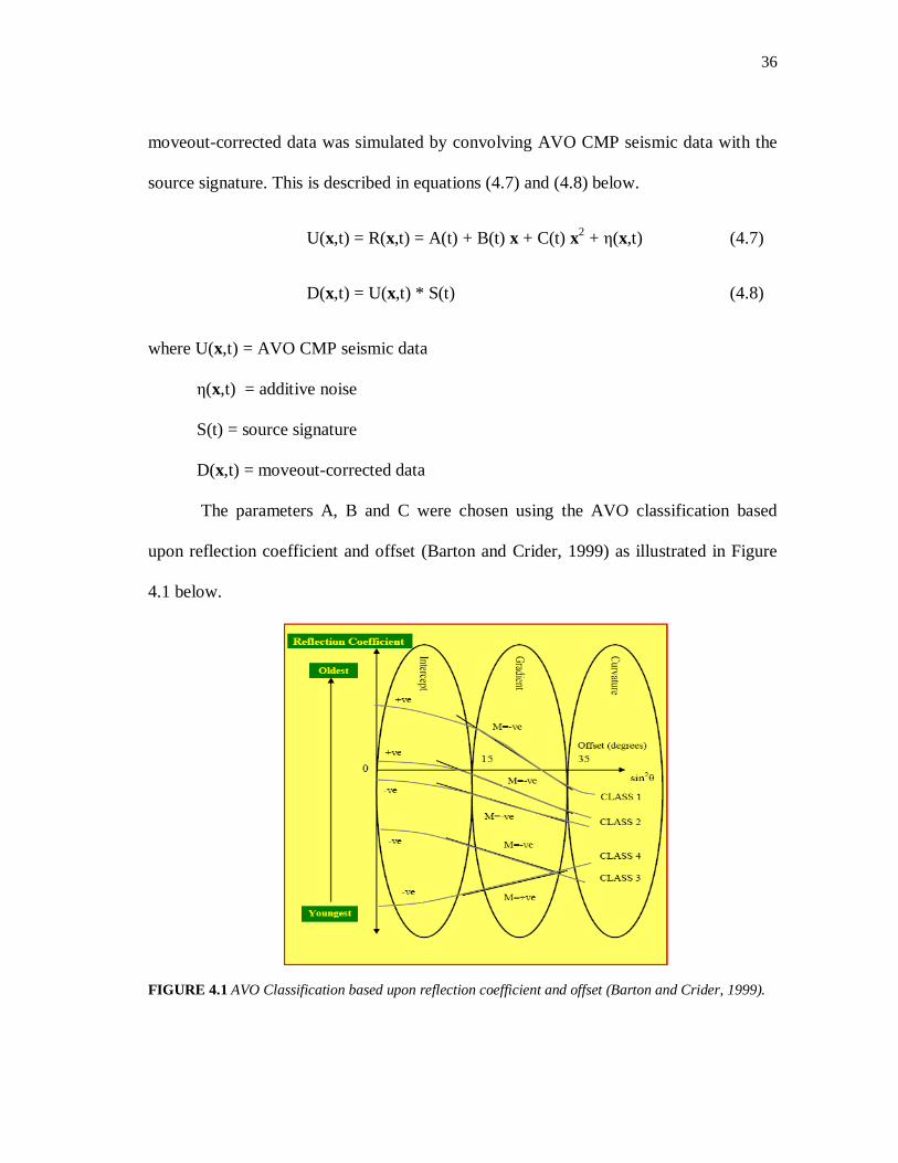
The parameters A, B and C were chosen using the AVO classification based

upon reflection coefficient and offset (Barton and Crider, 1999) as illustrated in Figure

4.1 below.

FIGURE 4.1 AVO Classification based upon reflection coefficient and offset (Barton and Crider, 1999).

37

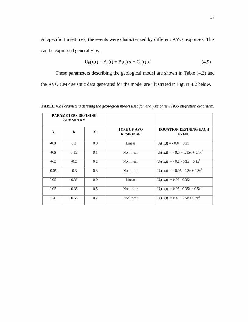
At specific traveltimes, the events were characterized by different AVO responses. This

can be expressed generally by:

Uk(x,t) = Ak(t) + Bk(t) x + Ck(t) x2 (4.9)

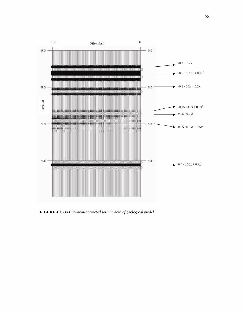
These parameters describing the geological model are shown in Table (4.2) and

the AVO CMP seismic data generated for the model are illustrated in Figure 4.2 below.

TABLE 4.2 Parameters defining the geological model used for analysis of new HOS migration algorithm.

PARAMETERS DEFINING GEOMETRY

A B C TYPE OF AVO

RESPONSE EQUATION DEFINING EACH

EVENT

-0.8 0.2 0.0 Linear U1( x,t) = - 0.8 + 0.2x

-0.6 0.15 0.1 Nonlinear U2( x,t) = - 0.6 + 0.15x + 0.1x2

-0.2 -0.2 0.2 Nonlinear U3( x,t) = - 0.2 - 0.2x + 0.2x2

-0.05 -0.3 0.3 Nonlinear U4( x,t) = - 0.05 - 0.3x + 0.3x2

0.05 -0.35 0.0 Linear U5( x,t) = 0.05 - 0.35x

0.05 -0.35 0.5 Nonlinear U6( x,t) = 0.05 - 0.35x + 0.5x2

0.4 -0.55 0.7 Nonlinear U7( x,t) = 0.4 - 0.55x + 0.7x2

38

FIGURE 4.2 AVO moveout-corrected seismic data of geological model.

Offset (km) 0.25 0 T

ime

(s)

-0.8 + 0.2x

-0.6 + 0.15x + 0.1x2

0.05 - 0.35x + 0.5x2

0.4 - 0.55x + 0.7x2

0.05 - 0.35x

-0.2 - 0.2x + 0.2x2

-0.05 - 0.3x + 0.3x2

39

Examples of HOS Migration

For the purposes of this investigation three examples are consided using the

geological model described above. In the first example, no noise is added to the events.

In the second example, Gaussian noise is added to each event. And in the final example,

different types of noise are added to the events. For each case the statistics, i.e. the mean,

variance, skewness and kurtosis are computed following the equations defined in Table

4.1. This is illustrated in Figures 4.3 to 4.5 respectively.

Analysis of Results

In the first example (Figure 4.3), no significant noise is added in this case. All

layers are well resolved by the mean as one might expect. The variance is quite small in

this case. Therefore the plot associated with it may not be that important. However, we

can notice that the portion of the data with significant interference produces a large

variance. This result is consistent with the fact that the amplitude may vary over a large

range in this area. The skewness is zero for the events with linear AVO response. This is

so because the data is uniform and therefore symmetric as observed in the previous

chapter. Notice that kurtosis is essentially negative in this example, which is consistent

with the fact that data without noise tends more to sub-Gaussian.

Now, in the second example (Figure 4.4), we have added Gaussian noise to the

data. Basically, the results are essentially unchanged except for the last event which has

a large AVO curvature and is therefore non-Gaussian. This combination with Gaussian

noise produces a slightly positive kurtosis.

40

EXAMPLE 1: NO NOISE ADDED

FIGURE 4.3 AVO moveout-corrected seismic data used for example 1 and the corresponding statistical

averages.

MEAN, M(x) VARIANCE, V(x)

SKEWNESS, S(x) KURTOSIS, K(x)

Offset (km)

Tim

e (

s)

0 0.25

Tim

e (

s)

Tim

e (

s)

AVO MOVEOUT-CORRECTED SEISMIC DATA OF GEOLOGICAL MODEL FOR EXAMPLE 1

Tim

e (

s)

Tim

e (s

)

0

0 0

0

1

2

0.5

0

1 - 0.5

1

2

0 0.02 0.060.04 0.08

2

1 1

2

0

0.02-0.02 -0.04

0

0.02

-0.02

-0.04 -0.08

41

EXAMPLE 2: GAUSSIAN NOISE ADDED


averages.



Offset (km) 0 0.25


Tim

e (

s)

0

0 0 0.04 -0.04 -0.08

0 0

0 0

1 1

1 1

2 2

2 2

0.5 -0.5 1 0 0.1 0.05

0.02 -0.02 -0.04

Tim

e (s

)

Tim

e (s

)

Tim

e (s

)

Tim

e (s

)

42

EXAMPLE 3: DIFFERENT TYPES OF NOISE ADDED


averages.



Offset (km) 0 0.25


Tim

e (

s)

Laplacian

Laplacian

Gaussian

Gaussian

Uniform

Uniform

Uniform

0.5 1 -0.5 0

0 0

0

1 1

1 1

0

2

2 2

2

0.1 0.2 0.3 0

0.04 0.08 -0.04 0.1 0.2 -0.1 0

Tim

e (s

) T

ime

(s)

Tim

e (s

) T

ime

(s)

43

In the final example (Figure 4.5), we have added different types of noise. The

noise component varies with time and includes both Gaussian and non-Gaussian noise,

with the non-Gaussian noise being either Uniform or Laplacian. For the first two events

in the data, the noise is Laplacian and we can see that the kurtosis has captured well this

information with the positive kurtosis (super Gaussian). The middle events with Uniform

noise can clearly captured with the negative kurtosis (sub Gaussian). For the last event,

we have Gaussian noise and nonlinear AVO behavior. In this case it is still not clear how

to define the result which can be sub Gaussian or super Gaussian.

44

CHAPTER V

SUMMARY AND CONCLUSIONS

The main motivation for the use of HOS in seismic imaging is the fact that many

signals in real life cannot be accurately modeled using the traditional 2nd order measures.

How accurately seismic imaging can be done depends on both the quality of the sensing

equipment and also very much on the effectiveness of the mathematical algorithms that

are used. Hence it is important when seismic imaging algorithms are improved.

If seismic modeling and imaging are to be improved, then more of the information

available in the data must be extracted and used. The examples presented confirm that

extra information carried by HOS can be obtained using my algorithm over conventional

imaging algorithms.

The mean attribute produces the same results as the present imaging technique

known as stack, whereas variance, skewness and kurtosis allow us to detect and

characterize linear and non-linear AVO behavior and the non-Gaussianity of the data.

Using skewness and kurtosis allows for the identification of the transition from

Gaussianity to non-Gaussianity, which coincides with the onset of the seismic event

despite noise presence. Skewness and kurtosis establish an effective statistical test in

identifying signals with asymmetrical distributions and nonlinear AVO behavior. The

simplicity of the method makes it an attractive candidate for huge seismic data

assessment in a real time context.

Another important conclusion is that there is a significant improvement in the

computation time, accuracy and the cost of seismic data processing, because the single

45

algorithm allows for the output of three parameters, the variance, skewness and kurtosis,

simultaneously and because we are avoiding errors associated with converting offsets to

angles when analyzing the AVO behavior. Furthermore, we will also be improving the

resolution of the seismic data since knowledge of the reflection angles is not necessary to

retrieve AVO information.

Hence it is recommended that HOS be employed as a tool in the assessment of

seismic data during the processing stage in seismic imaging.

46

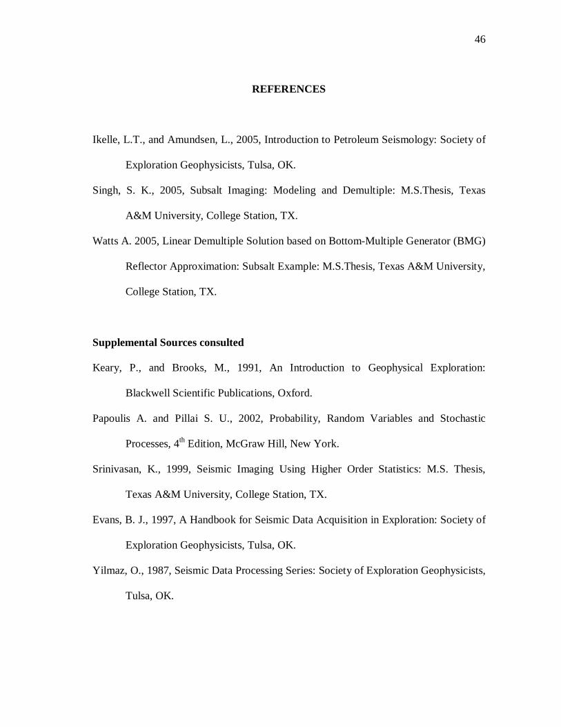
REFERENCES

Ikelle, L.T., and Amundsen, L., 2005, Introduction to Petroleum Seismology: Society of

Exploration Geophysicists, Tulsa, OK.

Singh, S. K., 2005, Subsalt Imaging: Modeling and Demultiple: M.S.Thesis, Texas

A&M University, College Station, TX.

Watts A. 2005, Linear Demultiple Solution based on Bottom-Multiple Generator (BMG)

Reflector Approximation: Subsalt Example: M.S.Thesis, Texas A&M University,

College Station, TX.

Supplemental Sources consulted

Keary, P., and Brooks, M., 1991, An Introduction to Geophysical Exploration:

Blackwell Scientific Publications, Oxford.

Papoulis A. and Pillai S. U., 2002, Probability, Random Variables and Stochastic

Processes, 4th Edition, McGraw Hill, New York.

Srinivasan, K., 1999, Seismic Imaging Using Higher Order Statistics: M.S. Thesis,

Texas A&M University, College Station, TX.

Evans, B. J., 1997, A Handbook for Seismic Data Acquisition in Exploration: Society of

Exploration Geophysicists, Tulsa, OK.

Yilmaz, O., 1987, Seismic Data Processing Series: Society of Exploration Geophysicists,

Tulsa, OK.

47

APPENDIX A

RANDOM VARIABLES, MOMENTS AND CUMULANTS

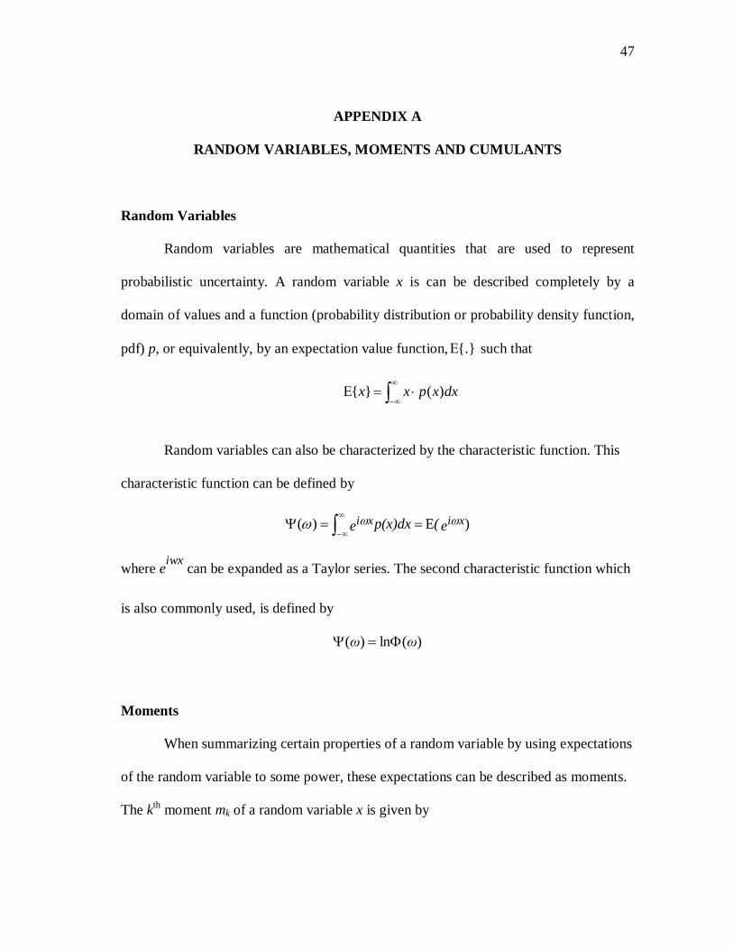
Random Variables

Random variables are mathematical quantities that are used to represent

probabilistic uncertainty. A random variable x is can be described completely by a

domain of values and a function (probability distribution or probability density function,

pdf) p, or equivalently, by an expectation value function, {.}Ε such that

Random variables can also be characterized by the characteristic function. This

characteristic function can be defined by

)E)( e( p(x)dxe xixi ωωω ==Ψ ∫∞

∞−

where eiwx

can be expanded as a Taylor series. The second characteristic function which

is also commonly used, is defined by

)(ln)( ωω Φ=Ψ

Moments

When summarizing certain properties of a random variable by using expectations

of the random variable to some power, these expectations can be described as moments.

The kth moment mk of a random variable x is given by

∫∞

∞−⋅=Ε dxxpxx )(}{

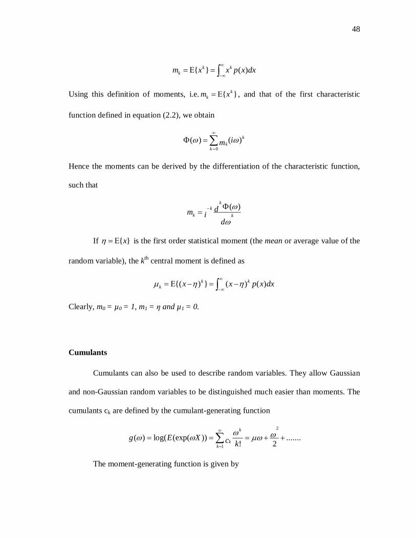
48

dxxpxxm kkk )(}{ ∫

∞

∞−=Ε=

Using this definition of moments, i.e. }{ kk xm Ε= , and that of the first characteristic

function defined in equation (2.2), we obtain

k

kk

im )()(0

ωω ∑∞

=

=Φ

Hence the moments can be derived by the differentiation of the characteristic function,

such that

ω

ω

d

dim k

kk

k

)(Φ=

−

If }{ xΕ=η is the first order statistical moment (the mean or average value of the

random variable), the kth central moment is defined as

∫∞

∞−−=−Ε= dxxpxx kk

k )()(}){( ηηµ

Clearly, m0 = µ0 = 1, m1 = η and µ1 = 0.

Cumulants

Cumulants can also be used to describe random variables. They allow Gaussian

and non-Gaussian random variables to be distinguished much easier than moments. The

cumulants ck are defined by the cumulant-generating function

.......2!

))(exp(log()(2

1

++=== ∑∞

=

ωµωω

ωωkcXEg

k

kk

The moment-generating function is given by

49

))(exp(!

exp!

111

ωωωg

kc

kck

k

kk

kk

=

=+ ∑∑

∞

=

∞

=

The cumulant-generating function is the logarithm of the moment generating function.

The cumulants are given by derivatives (at zero) of g(ω)

ck = g(k)(0)

e.g. c1 = µ = g'(0), c2 = σ2 = g''(0)

The cumulants of a distribution are closely related to distribution's moments. The

first cumulant is the expected value; the second and third cumulants are respectively the

second and third central moments (the second central moment is the variance); but the

higher cumulants are neither moments nor central moments, but rather more complicated

polynomial functions of the moments. Working with cumulants can have an advantage

over using moments because for independent variables X and Y,

))(log())(log())(log()).(log())(log()( )( wYwXwYwXYXw

YXeeeeeg Ε+Ε=ΕΕ=Ε= +

+ω

i.e. )()()( ωωω ggg YXYX

+=+

so that each cumulant of a sum is the sum of the corresponding cumulants of the

addends. More generally, we can rewrite equation (x) as:

ck(X + Y) = ck(X) + ck(Y)

This property of cumulants is known as additivity.

A more formal definition of the cumulants can be given in terms the second

characteristic function of a probability distribution, as defined above. Similar to

moments,

50

k

kk

ic )()(0

ωω ∑∞

=

=Ψ

The cumulants ck can therefore be defined by the relation,

ω

ω

d

dic k

kk

k

)(lnΦ=

−

Variance, Skewness, Kurtosis

The variance or dispersion of a distribution indicates the spread of the

distribution with respect to the mean value. It can be defined as follows:

∫∞

∞−−=−Ε= dxxpxx )()(}){( 222 ηησ

A lower value of variance indicates that the distribution is concentrated close to the

mean value, and a higher value indicates that the distribution is spread out over a wider

range of possible values.

The skewness of a distribution indicates the asymmetry of the distribution around

its mean, characterizing the shape of the distribution. It is given by

∫∞

∞−−=−Ε= dxxpxx )()(

1}){(

1 33

331 η

ση

σγ

The distribution, i.e. dataset, is symmetric if it looks the same to the left and right of the

peak point. The skewness for a normal distribution is zero and any symmetric data

should also have skewness near zero. A positive value of skewness indicates that the

distribution is skewed towards values greater than the mean (i.e., skewed towards the

51

right side) and a negative value indicates that the distribution is skewed towards the left

side.

The kurtosis of a distribution indicates the flatness of the distribution with

respect to the normal distribution. It is given by

∫∞

∞−−=−Ε= dxxpxx )()(

1}){(

1 44

442 η

ση

σγ

Positive kurtosis indicates a peaked distribution, whereas negative kurtosis indicates a

flat distribution. Distributions with positive kurtosis are sometimes termed super

Gaussian and distributions with negative kurtosis are sometimes termed sub Gaussian.

Kurtosis can be considered a measure of the non-Gaussianity of the random variable, x.

For a Gaussian random variable, kurtosis is zero, for a uniform distribution it is negative

and for a Laplace distribution it is positive.

52

VITA Name: Janelle Greenidge

Address: #4 Eighth Street West

Cassleton Avenue, Trincity

Trinidad, W.I.

Email: [email protected]

Education: M.S., May 2008

Texas A&M University

Department of Geology and Geophysics

Thesis: Seismic Attribute Analysis Using Higher Order Statistics

Major: Geophysics

B.S., August 2000

University of the West Indies

Department of Physics

Research Project: Electroencephalography for Left Handed Persons

Major: Physics

Postgraduate Diploma, October 2004

University of the West Indies

Department of Chemical Engineering

Petroleum Engineering Unit

Major: Petroleum Engineering

Documents

SEISMIC ATTRIBUTE ANALYSIS USING HIGHER ORDER …