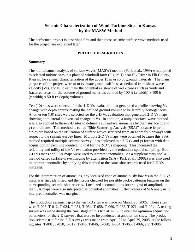
Seismic Characterization of Wind Turbine Sites in Kansas by the MASW Method

Choon B. Park and Richard D. Miller

Kansas Geological Survey University of Kansas

1930 Constant Avenue Lawrence, Kansas 66047-3726

Final Report to Rick Palm and Chris Kopchynski Barr Engineering Company 4700 West 77th Street Minneapolis, MN 55435-4803

Open File Report 2005-23 July 5, 2005

Contents at a Glance

Page PROJECT DESCRIPTION ------------------------------------------------------------------- 2-6

Summary General Acquisition Parameters 1-D Vs Profiling at Ten Selected Sites 2-D Surveys at Ten Selected Sites for Vs, SSA, and SIA Analyses Data Processing for 2-D Analyses and Voids Interpretations

DESCRIPTION OF METHODS USED --------------------------------------------------- 6-10 General Procedure with MASW Method for 1-D Vs Profile Key Acquisition Parameters for 1-D Vs Profile 2-D Shear-Wave Velocity (Vs) Mapping Side Scattering Analysis (SSA) Surface-Wave Imaging by Attenuation (SIA)

ACKNOWLEDGMENTS -----------------------------------------------------------------------10 REFERENCES -------------------------------------------------------------------------------- 10-11 TABLES ---------------------------------------------------------------------------------------- 12-14

Table 1: Shear-wave velocity (Vs) values obtained from MASW analysis at each site Table 2: Average Vs at ten 1-D sites, Elk County, Kansas Table 3: Average Vs at ten 2-D sites, Elk County, Kansas Table 4: Summary table of potential voids Table 5: Optimum acquisition parameters—Rules of thumb

FIGURES -------------------------------------------------------------------------------------- 15-30 APPENDICES

APPENDIX I: Maps from 2-D Shear-Wave Velocity (Vs) Analysis APPENDIX II: Side Scattering Analysis (SSA) APPENDIX III: Surface-Wave Imaging by Attenuation (SIA) APPENDIX IV: Bedrock (Vs > 500 m/sec) Topography

1

Seismic Characterization of Wind Turbine Sites in Kansas by the MASW Method

The performed project is described first and then those seismic surface-wave methods used for the project are explained later.

PROJECT DESCRIPTION Summary The multichannel analysis of surface waves (MASW) method (Park et al., 1999) was applied to selected turbine sites in a planned windmill farm (Figure 1) near Elk River in Elk County, Kansas, for seismic characterization of the upper 15 m or so of ground materials. The main purposes of the project were a) to evaluate ground stiffness as deduced from shear-wave velocity (Vs), and b) to estimate the potential existence of weak zones such as voids and fractured areas for the volume of ground materials defined by 100 ft (x-width) x 100 ft (y-width) x 50 ft (z-depth) volumes. Ten (10) sites were selected for the 1-D Vs evaluation that generated a profile showing Vs change with depth approximating the defined ground volume to be laterally homogeneous. Another ten (10) sites were selected for the 2-D Vs evaluation that generated 2-D Vs maps showing both lateral and vertical change in Vs. In addition, a unique surface-wave method was also applied to these 2-D sites to delineate subsurface anomalies by their surface (x and y) coordinates. This method is called “Side Scattering Analysis (SSA)” because its prin-ciples are based on the utilization of surface waves scattered from an anomaly sideways with respect to the seismic-survey lines. Multiple 2-D Vs maps were obtained because this SSA method required multiple seismic-survey lines deployed in a 2-D (x and y) format with data acquisition of each line identical to that for the 2-D Vs mapping. This increased the reliability and utility of the Vs evaluation provided by the redundant spatial sampling. Both 2-D Vs maps and SSA maps were used to interpret anomalies. As a supplementary tool a method called surface-wave imaging by attenuation (SIA) (Park et al., 1998a) was also used to interpret anomalies by applying this method to the same shot records used for 2-D Vs mapping. For the interpretation of anomalies, any localized zone of anomalously low Vs in the 2-D Vs maps was first identified and then cross checked for possible back-scattering features on the corresponding seismic-shot records. Localized accumulations (or troughs) of amplitude in the SSA maps were also interpreted as potential anomalies. Effectiveness of SIA analysis to interpret anomalies was marginal. The production seismic trip to the ten 1-D sites was made on March 28, 2005. These sites were T-003, T-012, T-024, T-031, T-054, T-058, T-060, T-065, T-071, and T-094. A testing survey was made during the final stage of this trip at T-065 to evaluate optimum acquisition parameters for the 2-D surveys that were to be conducted at another ten sites. The produc-tion seismic trip for the 2-D surveys was made from April 27 to April 29, 2005, at the follow-ing sites: T-001, T-010, T-017, T-040, T-046, T-060, T-064, T-065, T-066, and T-086.

2

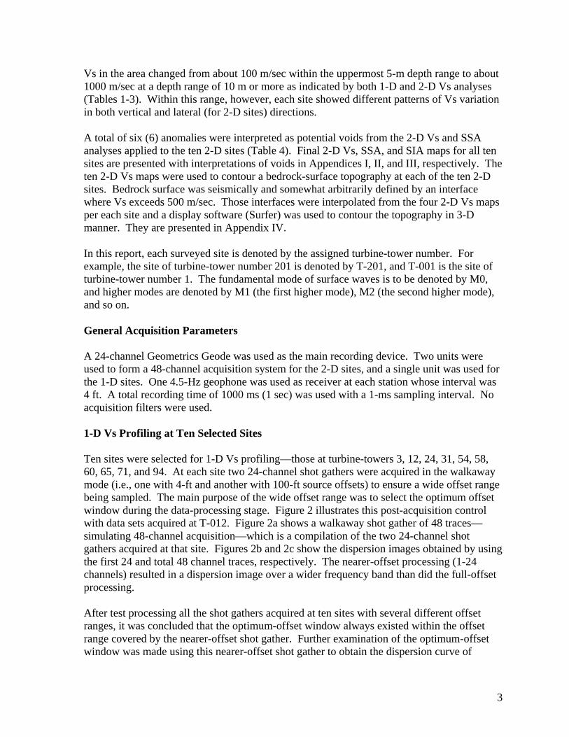
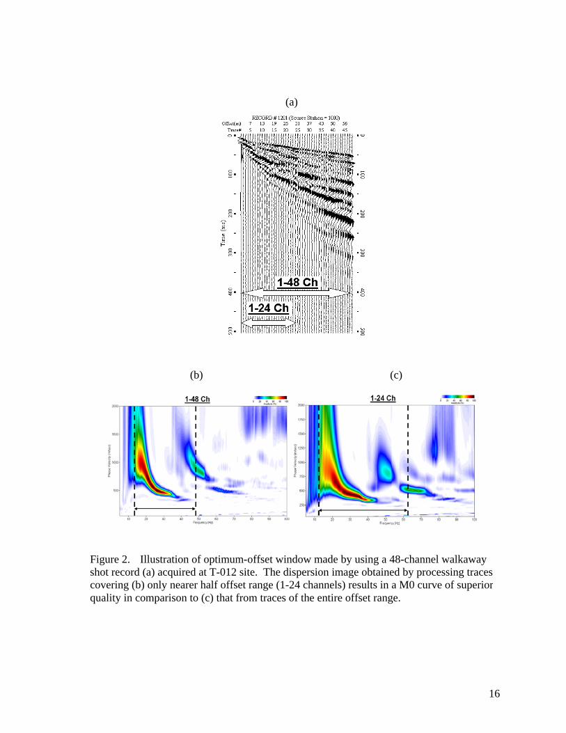
Vs in the area changed from about 100 m/sec within the uppermost 5-m depth range to about 1000 m/sec at a depth range of 10 m or more as indicated by both 1-D and 2-D Vs analyses (Tables 1-3). Within this range, however, each site showed different patterns of Vs variation in both vertical and lateral (for 2-D sites) directions. A total of six (6) anomalies were interpreted as potential voids from the 2-D Vs and SSA analyses applied to the ten 2-D sites (Table 4). Final 2-D Vs, SSA, and SIA maps for all ten sites are presented with interpretations of voids in Appendices I, II, and III, respectively. The ten 2-D Vs maps were used to contour a bedrock-surface topography at each of the ten 2-D sites. Bedrock surface was seismically and somewhat arbitrarily defined by an interface where Vs exceeds 500 m/sec. Those interfaces were interpolated from the four 2-D Vs maps per each site and a display software (Surfer) was used to contour the topography in 3-D manner. They are presented in Appendix IV. In this report, each surveyed site is denoted by the assigned turbine-tower number. For example, the site of turbine-tower number 201 is denoted by T-201, and T-001 is the site of turbine-tower number 1. The fundamental mode of surface waves is to be denoted by M0, and higher modes are denoted by M1 (the first higher mode), M2 (the second higher mode), and so on. General Acquisition Parameters A 24-channel Geometrics Geode was used as the main recording device. Two units were used to form a 48-channel acquisition system for the 2-D sites, and a single unit was used for the 1-D sites. One 4.5-Hz geophone was used as receiver at each station whose interval was 4 ft. A total recording time of 1000 ms (1 sec) was used with a 1-ms sampling interval. No acquisition filters were used. 1-D Vs Profiling at Ten Selected Sites Ten sites were selected for 1-D Vs profiling—those at turbine-towers 3, 12, 24, 31, 54, 58, 60, 65, 71, and 94. At each site two 24-channel shot gathers were acquired in the walkaway mode (i.e., one with 4-ft and another with 100-ft source offsets) to ensure a wide offset range being sampled. The main purpose of the wide offset range was to select the optimum offset window during the data-processing stage. Figure 2 illustrates this post-acquisition control with data sets acquired at T-012. Figure 2a shows a walkaway shot gather of 48 traces—simulating 48-channel acquisition—which is a compilation of the two 24-channel shot gathers acquired at that site. Figures 2b and 2c show the dispersion images obtained by using the first 24 and total 48 channel traces, respectively. The nearer-offset processing (1-24 channels) resulted in a dispersion image over a wider frequency band than did the full-offset processing. After test processing all the shot gathers acquired at ten sites with several different offset ranges, it was concluded that the optimum-offset window always existed within the offset range covered by the nearer-offset shot gather. Further examination of the optimum-offset window was made using this nearer-offset shot gather to obtain the dispersion curve of

3

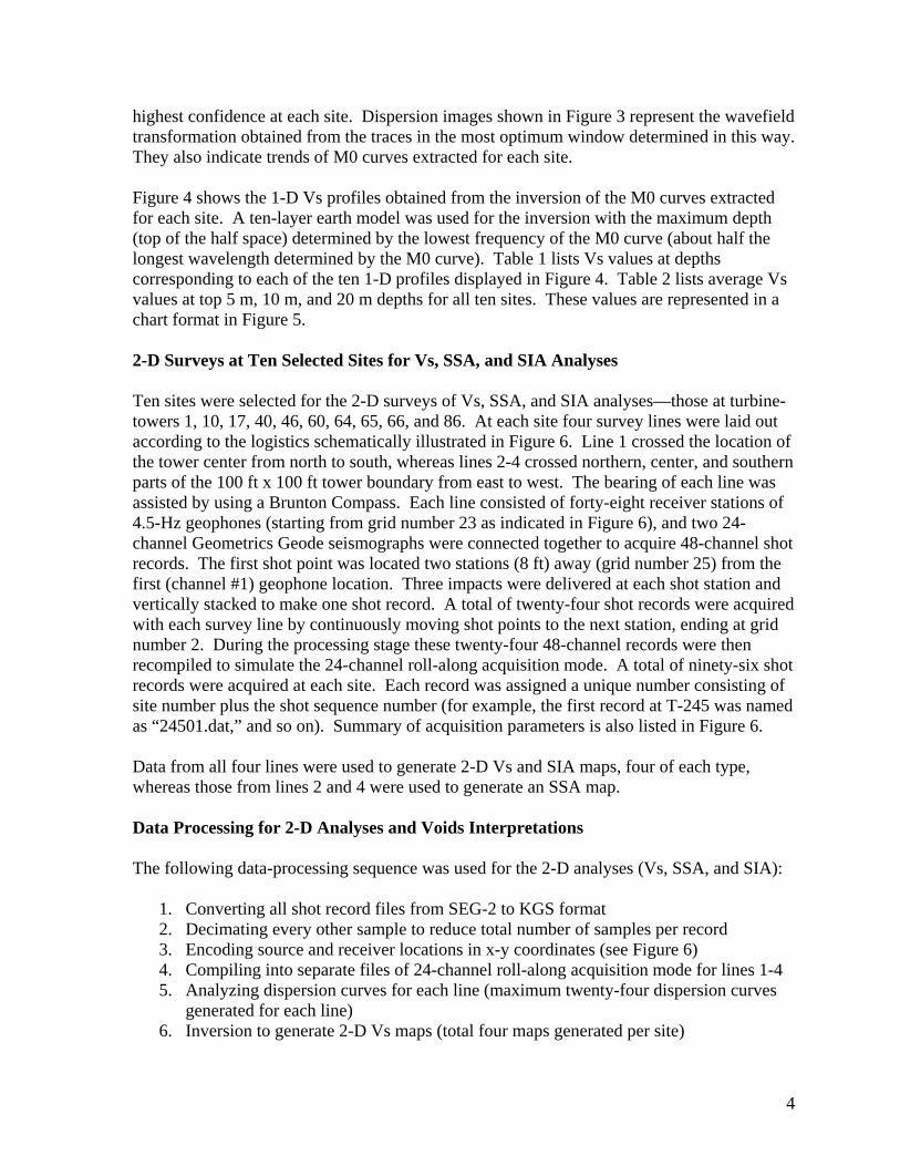
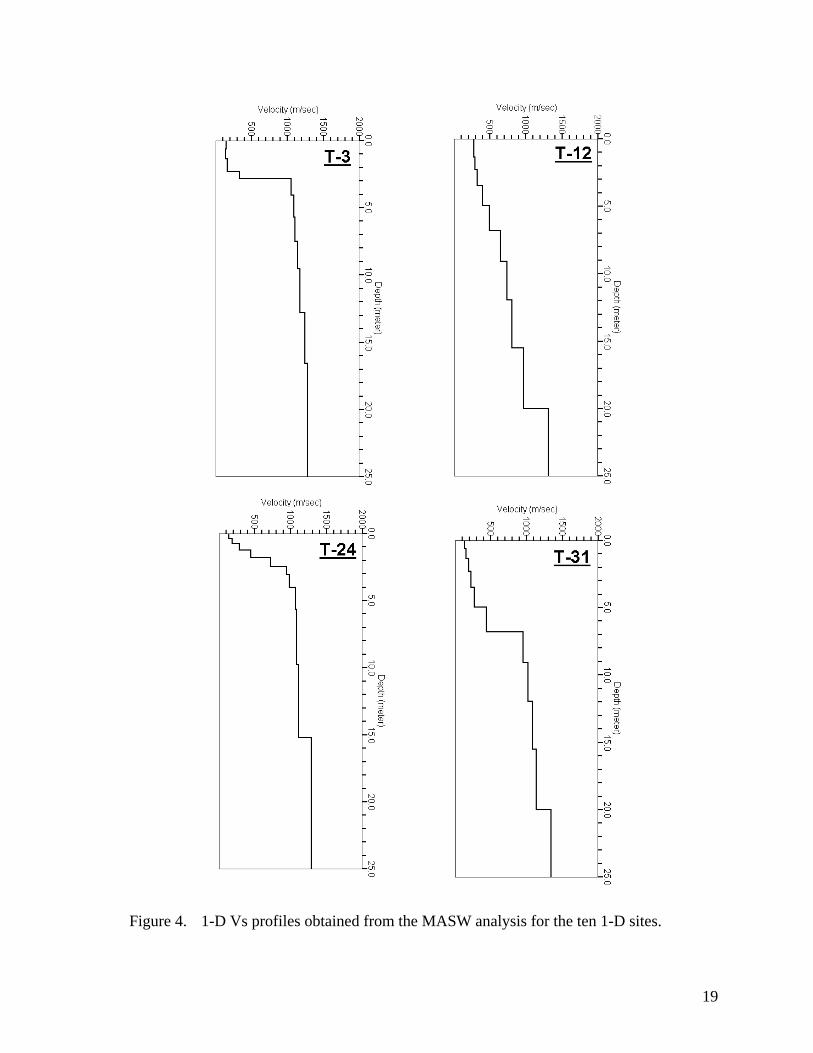
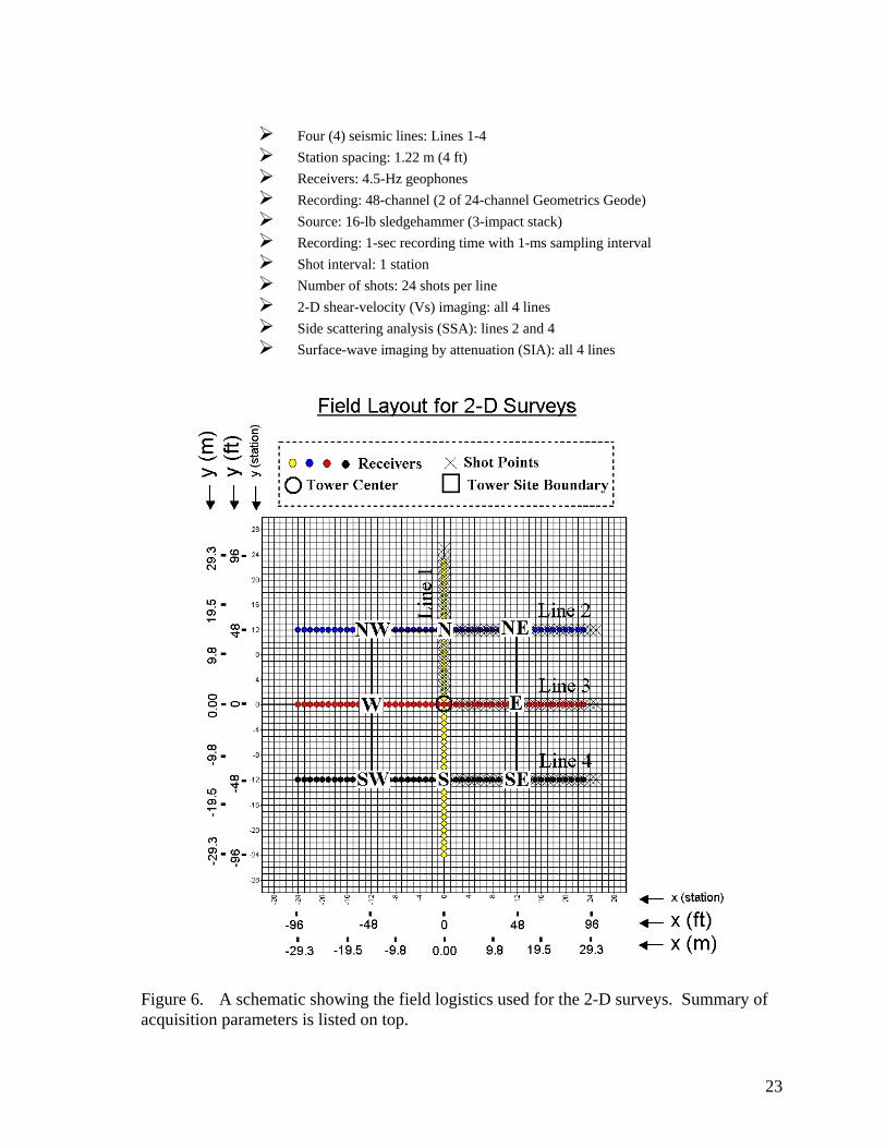
highest confidence at each site. Dispersion images shown in Figure 3 represent the wavefield transformation obtained from the traces in the most optimum window determined in this way. They also indicate trends of M0 curves extracted for each site. Figure 4 shows the 1-D Vs profiles obtained from the inversion of the M0 curves extracted for each site. A ten-layer earth model was used for the inversion with the maximum depth (top of the half space) determined by the lowest frequency of the M0 curve (about half the longest wavelength determined by the M0 curve). Table 1 lists Vs values at depths corresponding to each of the ten 1-D profiles displayed in Figure 4. Table 2 lists average Vs values at top 5 m, 10 m, and 20 m depths for all ten sites. These values are represented in a chart format in Figure 5. 2-D Surveys at Ten Selected Sites for Vs, SSA, and SIA Analyses Ten sites were selected for the 2-D surveys of Vs, SSA, and SIA analyses—those at turbine-towers 1, 10, 17, 40, 46, 60, 64, 65, 66, and 86. At each site four survey lines were laid out according to the logistics schematically illustrated in Figure 6. Line 1 crossed the location of the tower center from north to south, whereas lines 2-4 crossed northern, center, and southern parts of the 100 ft x 100 ft tower boundary from east to west. The bearing of each line was assisted by using a Brunton Compass. Each line consisted of forty-eight receiver stations of 4.5-Hz geophones (starting from grid number 23 as indicated in Figure 6), and two 24-channel Geometrics Geode seismographs were connected together to acquire 48-channel shot records. The first shot point was located two stations (8 ft) away (grid number 25) from the first (channel #1) geophone location. Three impacts were delivered at each shot station and vertically stacked to make one shot record. A total of twenty-four shot records were acquired with each survey line by continuously moving shot points to the next station, ending at grid number 2. During the processing stage these twenty-four 48-channel records were then recompiled to simulate the 24-channel roll-along acquisition mode. A total of ninety-six shot records were acquired at each site. Each record was assigned a unique number consisting of site number plus the shot sequence number (for example, the first record at T-245 was named as “24501.dat,” and so on). Summary of acquisition parameters is also listed in Figure 6. Data from all four lines were used to generate 2-D Vs and SIA maps, four of each type, whereas those from lines 2 and 4 were used to generate an SSA map. Data Processing for 2-D Analyses and Voids Interpretations The following data-processing sequence was used for the 2-D analyses (Vs, SSA, and SIA):

1. Converting all shot record files from SEG-2 to KGS format 2. Decimating every other sample to reduce total number of samples per record 3. Encoding source and receiver locations in x-y coordinates (see Figure 6) 4. Compiling into separate files of 24-channel roll-along acquisition mode for lines 1-4 5. Analyzing dispersion curves for each line (maximum twenty-four dispersion curves

generated for each line) 6. Inversion to generate 2-D Vs maps (total four maps generated per site)

4

7. Selecting a reference dispersion curve for SSA processing (usually the curve obtained from the record whose receiver spread was centered at the tower center in line 1)

8. Generating one SSA map 9. Generating four (lines 1-4) SIA maps using the same reference dispersion curve used

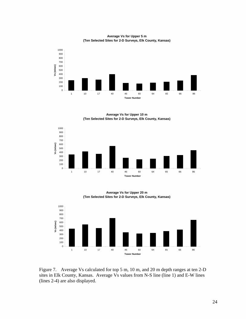
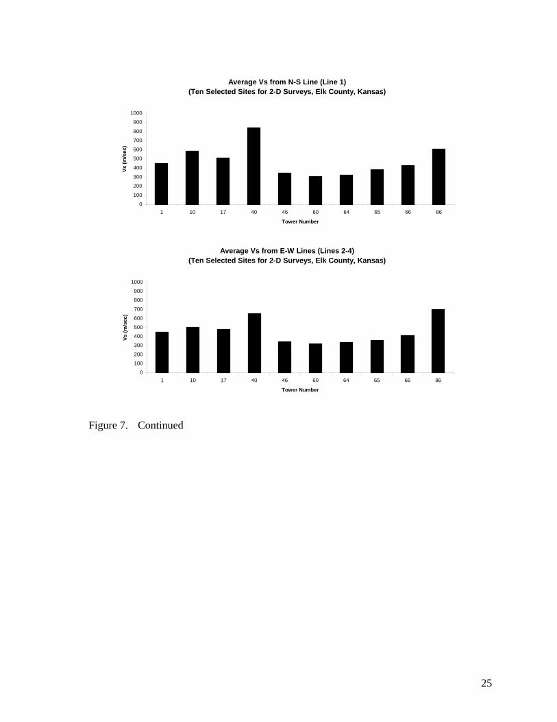
for SSA analysis. Dispersion curves were first automatically extracted by using an algorithm that follows the energy trends and then manually edited by discarding those outliers not fitting into a reasonable trend and also by adding those points that could not be automatically picked due to weak energy. Most of the extracted curves were in the frequency range of 10-60 Hz with the phase velocities in 100 m/sec – 1000 m/sec. Inversion of the extracted dispersion curves was performed using the algorithm by Xia et al. (1999). A ten-varying-thickness layer model was created at the beginning of the inversion with the maximum depth (Zmax) (top of the half space) being about 50% of the longest wavelength. Zmax was usually in the range of 20-30 m. Initial Vs model was created with an aid of phase velocity versus wavelength relationship depicted by the dispersion curve. Poisson’s ratio of 0.3 and density of 2.0 gr/cc were assigned for all ten layers during the inversion process. The iterative inversion was forced to stop after the fifth iteration of updating the Vs model. This relatively small number of iterations was chosen to minimize the effect of computational artifacts. Side Scattering Analysis (SSA) was applied to records of lines 2 and 4 by using a reference dispersion curve for a square (20 m x 20 m) surface (x and y) area (Figure 6) with a grid interval of 0.2 m. The reference dispersion curve was chosen among those obtained near the tower center that had an M0 curve best defined for wavelengths shorter than 20 m so that the depth of sensitivity was focused into 0-10 m. Surface-wave Imaging by Attenuation (SIA) analysis was applied to records of all four lines (lines 1-4) by using another reference curve chosen among those near the tower center that had the greatest range of wavelengths so that the sensitivity depth could be maximized. One 2-D map was obtained from records of one seismic line, totaling four maps per site. To interpret anomalies, first any localized zone of anomalously low velocities in the 2-D Vs maps was identified, then cross checked for possible back-scattering features on the corresponding seismic-shot records. Localized accumulations (or troughs) of amplitude in the SSA maps were also interpreted as potential anomalies. Effectiveness of the SIA analysis to interpret anomalies was marginal. A summary of interpreted anomalies (voids) is listed in Table 4. Final 2-D Vs, SSA, and SIA maps for all ten sites are presented with interpretations of voids in Appendices I, II, and III, respectively. Vs values obtained from all four lines at each site were averaged for top 5 m, 10 m, and 20 m depth ranges. These values are listed in Table 3 and represented in a chart format in Figure 7. Also, average Vs values from N-S line (line 1) and E-W lines (lines 2-4) were separately obtained for a possible study of seismic anisotropy in association with any regional lineation features in the area. 2-D Vs maps were used to contour a bedrock-surface topography at each of the ten 2-D sites. Bedrock surface was seismically and somewhat arbitrarily defined by an interface where Vs exceeds 500 m/sec. Those interfaces were interpolated from the four 2-D Vs maps per each

5

site and a display software (Surfer) was used to contour the topography in 3-D manner. They are presented in Appendix IV. Because the data points for the displays were sampled not from a regularly designed grid system, any localized undulations should be interpreted with caution and only the regional trend of the bedrock surface may contain the greatest reliability.

DESCRIPTION OF METHODS USED A detailed description of the theory of the multichannel analysis of surface waves (MASW) method and typical field application can be found in Park et al. (1999), Xia et al. (1999), and Miller et al. (1999). General Procedure with MASW Method for 1-D Vs Profile A multiple number of receivers (usually 24 or more) are deployed with even spacing along a linear survey line with receivers connected to a multichannel recording device (seismograph) (Figure 8). Each channel is dedicated to recording vibrations from one receiver. One multichannel record (commonly called a shot gather) consists of a multiple number of time series (called traces) from all the receivers in an ordered manner. Data processing consists of three steps (Figure 9): 1) preliminary detection of surface waves, 2) constructing the dispersion image panel and extracting the signal dispersion curve, and 3) back-calculating Vs variation with depth. All these steps can be fully automated. The pre-liminary detection of surface waves examines recorded seismic waves in the most probable range of frequencies and phase velocities. Construction of the image panel is accomplished through a 2-D (time and space) wavefield transformation method that employs several pattern-recognition approaches (Park et al., 1998b). This transformation eliminates all the ambient cultural noise as well as source-generated noise such as scattered waves from buried objects (building foundations, culverts, boulders, etc.). The image panel shows the relation-ship between phase velocity and frequency for those waves propagated horizontally and directly from the impact point to the receiver line. These waves include fundamental and higher modes of surface waves as well as direct (compressional) body waves (Figure 9b). The necessary dispersion curve, such as that of fundamental-mode Rayleigh waves, is then extracted from the energy accumulation pattern in this image panel (Figure 9b). The extracted dispersion curve is finally used as a reference to back-calculate the Vs variation with depth below the surveyed area. This back-calculation is called inversion and the process can be automated with reasonable constraints (Xia et al., 1999). Key Acquisition Parameters for 1-D Vs Profile Unlike other seismic methods (e.g., reflection or refraction), acquisition parameters for MASW surveys have quite a wide range of tolerance. This is because the multichannel pro-cessing schemes employed in the wavefield transformation method (Park et al., 1998b) have the capability to automatically account for such otherwise adverse effects as near-field, far-field, and spatial aliasing effects (Park et al., 1999). Nevertheless, two types of parameters are considered to be most important: the source offset (x1) and the receiver spacing (dx)

6

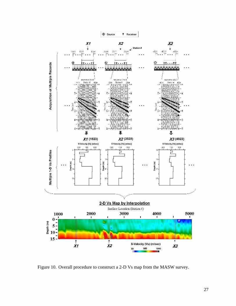
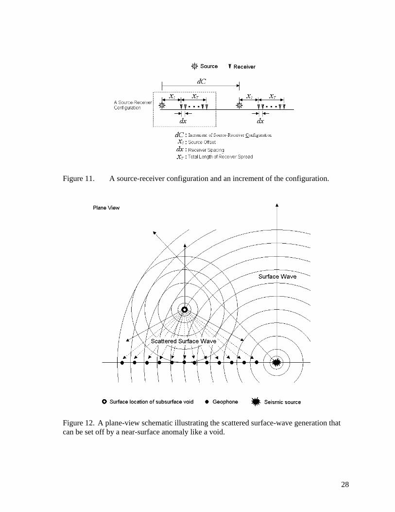
(Figure 8). The source offset (x1) needs to change in proportion to the maximum investiga-tion depth (zmax). A conservative rule of thumb would be x1 = γzmax with γ=0.5. However, very often γ can be as small as 0.1 (Park et al., 1999). The receiver spacing (dx) may need to be slightly dependent on the average stiffness of near-surface materials. A rule of thumb is dx ≈ 1.0 m in most surveys over soil sites. Table 5 summarizes optimum ranges of all the acquisition parameters (Park et al., 2002). 2-D Shear-Velocity (Vs) Mapping A 2-D Vs map is constructed from the acquisition of multiple records (Figure 10) with a fixed source-receiver configuration and a fixed increment (dC) of the configuration (Figure 11). A source-receiver configuration indicates a setup of given source offset (x1), receiver spacing (dx), and total number of channels (N) used during a survey. The increment dC depends on the degree of horizontal variation in Vs along the entire survey line (Park, 2005). A small increment would be necessary if a high degree of horizontal variation is expected. In most cases where total receiver spread length (xT) is set in such a way that horizontal variation within xT can be ignored, an increment of half the spread would be sufficient: dC ≈ 0.5 xT. Therefore, determination of optimum xT has to be made before optimum dC is determined. In theory, a shorter xT would ensure a higher accuracy in handling the horizontal variation. However, it would also impede the accurate assessment of dispersion curves (Park et al., 2001). Therefore, there is a trade-off. In most soil-site applications, xT in the range of 10-30 m is most optimal and this gives an optimal dC in the range of 5-15 m.

Once multiple records (> 5) are acquired by regularly moving the source-receiver configura-tion, one 1-D Vs profile is obtained from each record through the surface-wave processing outlined previously. Each Vs profile also has the appropriate horizontal coordinate (i.e., station number) to represent the vertical Vs variation. Naturally, the midpoint of the receiver spread is used for this purpose. Multiple 1-D Vs profiles obtained are then used for a 2-D (x and z) interpolation to create the final 2-D map (Figure 10). Side Scattering Analysis (SSA) Surface waves are known to be sensitive to the presence of near-surface anomalies such as near-vertical fractures and voids. A significant amount of surface-wave energy impinging against them is transformed into scattered surface waves due to anomalies acting as new sources of surface waves (Figure 12). Therefore, MASW data collected for normal 2-D Vs mapping can also be used to detect possible anomalies existing subsurface off the survey line by using a processing scheme similar to the conventional reflection processing. This process is called a side-scattering analysis (SSA) of surface waves. A brief explanation of the processing scheme follows. When a void exists below a certain surface location (xv, yv), then a scattered surface-wave component of f-Hz traveling with a phase velocity of Cf generated by impact of a source located at (xs, ys) will reach a receiver point (xr, yr) at time δt(f) (Figure 13):

7

( )

( ) ( ) ( ) ( )222

221

21

and with

)(

vrvrvsvs

f

yyxxLyyxxL

CLLft

−+−=−+−=

+=δ

(1)

Based on this travel-time relationship, to evaluate the relative probability of a surface point being the source of such scattering, a plane (x-y) grid is first established within which the detection of subsurface anomalies is sought (Figure 13). Then, each point (xv, yv) in the grid is assumed to be the source of scattering. The corresponding scattered wavefields are then collapsed to their origin in time by applying an appropriate phase shift and then all those collapsed waves are summed (stacked) together to yield an indicator : ),( vv yxSSA

∑ ∑ −= traces sfrequencie

,)(2 )( ),( jfReyxSSA Norm

srftfj

vvδπ , (2)

where indicates the normalized Fourier transformation of seismic trace recorded by the receiver at (x

)(, jfR Normsr )(trs

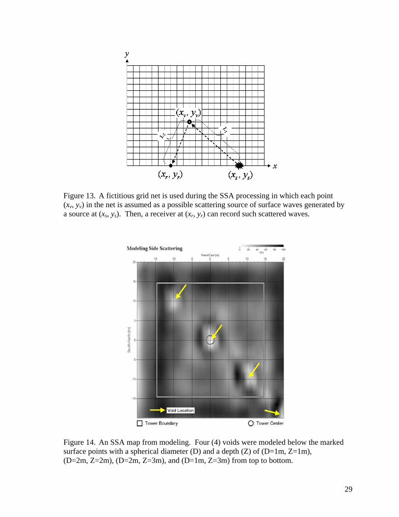
r, yr) when seismic source was located at (xs, ys). SSA is proportional to the intensity of scattering, therefore qualitatively the existence probability of an anomaly. Therefore, when these values of SSAs calculated at all the grid points are dis-played through a simple 2-D format, actual points of scattering will show peaks or troughs depending on whether there is a 180° phase shift at the time of scattering or not (Figure 14). In the modeling illustration in Figure 14, the 180° phase shift was assumed. Phase velocities (Cf’s) of a dispersion curve representative of the area are used in the calculation of δt(f). The depth range sensitive to this analysis is assumed to be half the range of wavelengths defined by the representative dispersion curve. For example, if the reference curve has phase velocities changing from 1000 m/sec at the lowest frequency of 20 Hz to 100 m/sec at the highest frequency of 100 Hz, then corresponding wavelengths change from 50 m to 1 m and the sensitive depth range of the SSA analysis becomes 25 m – 0.5 m. Sensitive depth range of SSA method is expected to be about the half the wavelengths used during the processing and the sensitive dimension (in diameter) of anomaly is expected to be about 10 % of its depth of existence. For example, if the reference curve had wavelengths in 4-20 m, then depth (z) of 2-10 m is sensitive for those anomalies larger than 0.2 m existing at z = 2 m, 0.5 m existing at z = 5 m, and so on. More details of this processing scheme will be available in near-future publications. Surface-Wave Imaging by Attenuation (SIA) A near-surface anomaly is defined here as that part of near-surface materials that have elastic properties significantly different from the surrounding study area. The transition from normal zone to anomaly zone may be either abrupt or gradual. During a surface wave survey, a near-surface anomaly will leave a signature of its presence on multichannel records in several forms. The most common signature is different phase

8

velocities for those frequencies propagating through or near the anomaly. Another form would be different attenuation characteristics. Besides different phase velocities and attenuation characteristics, an anomaly may reveal its presence through the generation of higher modes and reflected and diffracted surface waves. Generation of the higher modes becomes significant, especially in the case of velocity inver-sion and when energy of the higher modes tends to increase for high frequencies (Tokimatsu et al., 1992). Reflected and diffracted ground roll will be generated if the transition from normal zone to anomaly zone is abrupt. All these types of anomaly signatures may appear on a multichannel record when either the source or receivers are located at or near the surface location of the anomaly. Theoretically, surface waves cannot penetrate a void filled with air or fluid because of the lack of shear modulus inside the void. However, the bulk of mass experiencing the retrograde elliptical motion of surface waves increases as penetration depth increases. Therefore, surface waves with penetration depths greater than or comparable to the depth of the void will experience certain changes in either attenuation or phase velocity, or both. Based on the outlined principles, the data processing scheme for SIA analysis is briefly explained below. Dynamic linear move out (DLMO) correction is applied to each shot gather to correct for the offset effect, therefore, to flatten the linearly sloping events of surface waves (Park et al., 1996). The correction is a dynamic operation because the amount of correction changes with time as well as offset. DLMO can be accomplished in the frequency domain as follows:

(3) ),,(),( xfWj

exfW f

DLMO

Φ=

where = Fourier transform applied to time axis of a shot gather, , = Fourier transform of DLMO-corrected shot gather, , x = distance from source, =

),( xfW ),( xtw

),( xfWDLMO

),( xtwDLMO

fΦ fCfxπ2 , and

= phase velocity for frequency f.

fC

The velocity function C used in DLMO correction is calculated from a shot gather obtained at a reference location. The reference location is a presumably normal zone within the survey line. All traces in a DLMO-corrected shot gather are then stacked together to produce one stacked trace per shot.

f

After stacking, this procedure achieves the following: • Those frequencies that have phase velocity equivalent to that at the reference location

will have large stacked amplitudes through constructive interference. • For those shot gathers obtained at or near the surface location of an anomaly, DLMO

correction will result in stacked traces of weak amplitudes through destructive interfer-

9

ence for those frequencies that have penetration depths comparable to the depth of the anomaly.

• All the higher modes will be attenuated through destructive interference because of their different phase velocities.

• All nonplanar, reflected, and diffracted ground rolls (and possibly any body-wave events) will be attenuated through destructive interference because of their nonlinear occurrence on a multichannel record.

• Random noise will be attenuated. When stacked traces are displayed, all the normal zones will show large amplitudes and the anomalous zones will be denoted by attenuated amplitudes (Figure 15). The degree of attenu-ation will be proportional to the degree of being anomalous with respect to the reference location. Although a systematic study has not been performed yet, the sensitivity of the SIA method is expected to be much lower than that of the SSA method. More detailed description of SIA analysis can be found in Park et al. (1998a).

ACKNOWLEDGMENTS We would like to thank Tom Kjos from Mortenson Construction Company for his assistance with site locations during the field operations. Our sincere appreciation goes to many people involved in the preparation and the operation of field surveys; among them are David Thiel, Andrew Newell, and Nicolette Proudfoot. Also, David Laflen, Brett Bennett, and Mary Brohammer at the Kansas Geological Survey played critical roles in the background making necessary arrangements.

REFERENCES Miller, R.D., Xia, J., Park, C.B., and Ivanov, J., 1999, Multichannel analysis of surfaces

waves to map bedrock: The Leading Edge, v. 18, no. 12. Park, C.B., 2005, MASW⎯Horizontal resolution in 2-D shear-wave velocity (Vs) mapping:

Kansas Geological Survey, Open-file Report 2005-4. Park, C.B., Miller, R.D., and Miura, H., 2002, Optimum field parameters of an MASW

survey [Exp. Abs.]: SEG-J, Tokyo, May 22-23, 2002. Park, C.B., Miller, R.D., and Xia, J., 2001, Offset and resolution of dispersion curve in

multichannel analysis of surface waves (MASW): Proceedings of the SAGEEP 2001, Denver, Colorado, SSM-4.

Park, C.B., Miller, R.D., and Xia, J., 1999, Multi-channel analysis of surface waves

(MASW): Geophysics, v. 64, no. 3, p. 800-808. Park, C.B., Miller, R.D., and Xia, J., 1998a, Ground roll as a tool to image near-surface

anomaly [Exp. Abs.]: Soc. Explor. Geophys., p. 874-877.

10

Park, C.B., Miller, R.D., and Xia, J., 1998b, Imaging dispersion curves of surface waves on

multi-channel record [Exp. Abs.]: Soc. Explor. Geophys., p. 1377-1380. Park, C.B., Miller, R.D., and Xia, J., 1996, Multi-channel analysis of surface waves using

Vibroseis (MASWV) [Exp. Abs.]: Soc. Explor. Geophys., p. 68-71. Tokimatsu, K., Tamura, S., and Kojima, H., 1992, Effects of multiple modes on Rayleigh

wave dispersion characteristics: Journal of Geotechnical Engineering, American Society of Civil Engineering, v. 118, no. 10, p. 1529-1543.

Xia, J., Miller, R.D., and Park, C.B., 1999, Estimation of near-surface shear-wave velocity by

inversion of Rayleigh waves: Geophysics, v. 64, no. 3, p. 691-700.

11

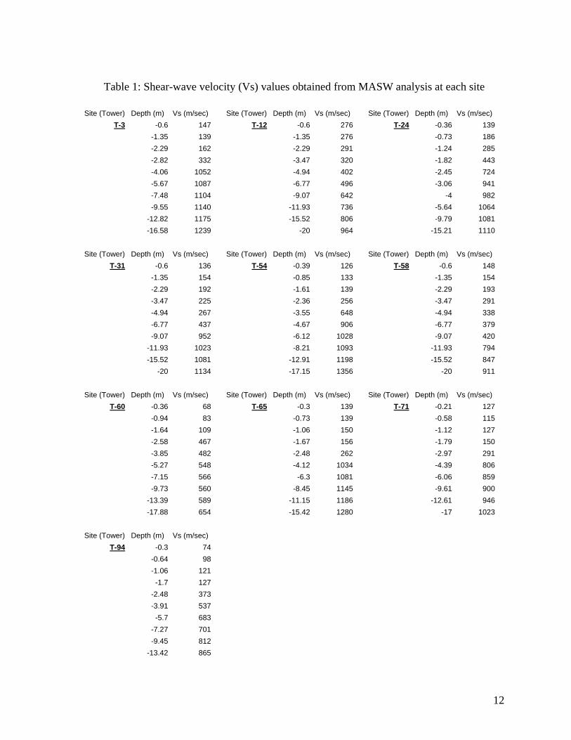
Table 1: Shear-wave velocity (Vs) values obtained from MASW analysis at each site

Site (Tower) Depth (m) Vs (m/sec) Site (Tower) Depth (m) Vs (m/sec) Site (Tower) Depth (m) Vs (m/sec)

T-3 -0.6 147 T-12 -0.6 276 T-24 -0.36 139 -1.35 139 -1.35 276 -0.73 186 -2.29 162 -2.29 291 -1.24 285 -2.82 332 -3.47 320 -1.82 443 -4.06 1052 -4.94 402 -2.45 724 -5.67 1087 -6.77 496 -3.06 941 -7.48 1104 -9.07 642 -4 982 -9.55 1140 -11.93 736 -5.64 1064 -12.82 1175 -15.52 806 -9.79 1081 -16.58 1239 -20 964 -15.21 1110

Site (Tower) Depth (m) Vs (m/sec) Site (Tower) Depth (m) Vs (m/sec) Site (Tower) Depth (m) Vs (m/sec)T-31 -0.6 136 T-54 -0.39 126 T-58 -0.6 148

-1.35 154 -0.85 133 -1.35 154 -2.29 192 -1.61 139 -2.29 193 -3.47 225 -2.36 256 -3.47 291 -4.94 267 -3.55 648 -4.94 338 -6.77 437 -4.67 906 -6.77 379 -9.07 952 -6.12 1028 -9.07 420 -11.93 1023 -8.21 1093 -11.93 794 -15.52 1081 -12.91 1198 -15.52 847 -20 1134 -17.15 1356 -20 911

Site (Tower) Depth (m) Vs (m/sec) Site (Tower) Depth (m) Vs (m/sec) Site (Tower) Depth (m) Vs (m/sec)T-60 -0.36 68 T-65 -0.3 139 T-71 -0.21 127

-0.94 83 -0.73 139 -0.58 115 -1.64 109 -1.06 150 -1.12 127 -2.58 467 -1.67 156 -1.79 150 -3.85 482 -2.48 262 -2.97 291 -5.27 548 -4.12 1034 -4.39 806 -7.15 566 -6.3 1081 -6.06 859 -9.73 560 -8.45 1145 -9.61 900 -13.39 589 -11.15 1186 -12.61 946 -17.88 654 -15.42 1280 -17 1023

Site (Tower) Depth (m) Vs (m/sec)

T-94 -0.3 74 -0.64 98 -1.06 121 -1.7 127 -2.48 373 -3.91 537 -5.7 683 -7.27 701 -9.45 812 -13.42 865

12

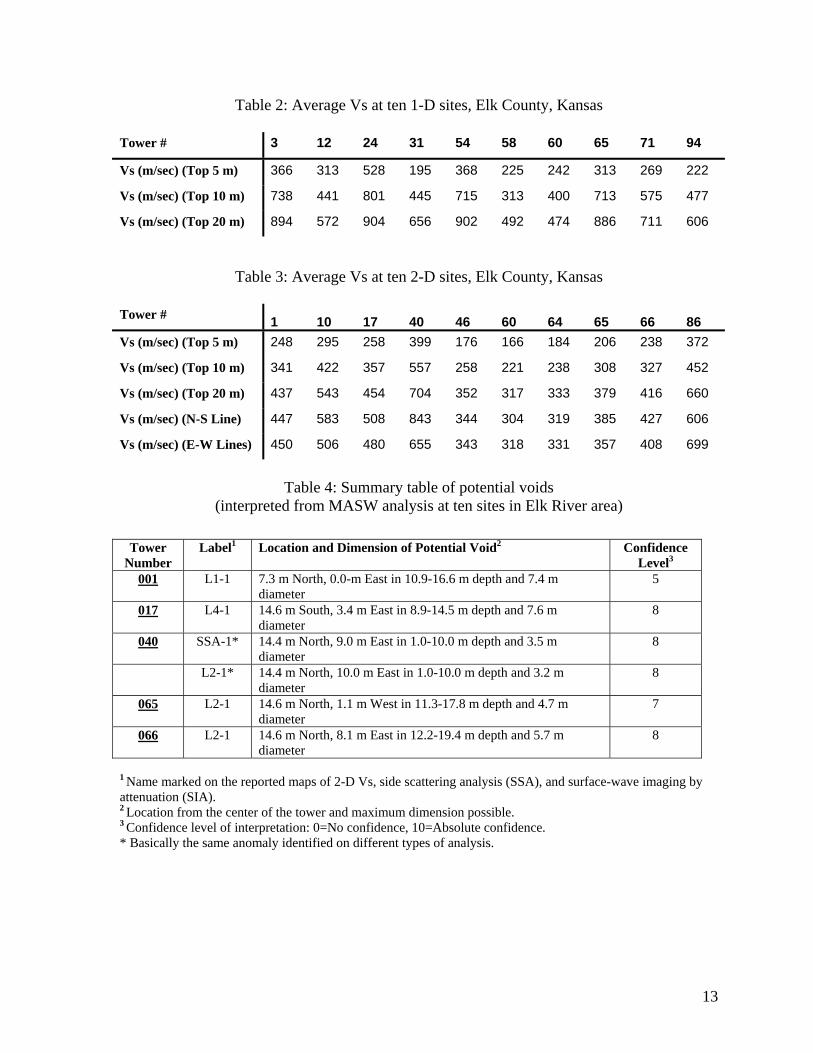
Table 2: Average Vs at ten 1-D sites, Elk County, Kansas Tower # 3 12 24 31 54 58 60 65 71 94

Vs (m/sec) (Top 5 m) 366 313 528 195 368 225 242 313 269 222

Vs (m/sec) (Top 10 m) 738 441 801 445 715 313 400 713 575 477

Vs (m/sec) (Top 20 m) 894 572 904 656 902 492 474 886 711 606

Table 3: Average Vs at ten 2-D sites, Elk County, Kansas Tower # 1 10 17 40 46 60 64 65 66 86 Vs (m/sec) (Top 5 m) 248 295 258 399 176 166 184 206 238 372

Vs (m/sec) (Top 10 m) 341 422 357 557 258 221 238 308 327 452

Vs (m/sec) (Top 20 m) 437 543 454 704 352 317 333 379 416 660

Vs (m/sec) (N-S Line) 447 583 508 843 344 304 319 385 427 606

Vs (m/sec) (E-W Lines) 450 506 480 655 343 318 331 357 408 699

Table 4: Summary table of potential voids

(interpreted from MASW analysis at ten sites in Elk River area)

Tower

Number Label1 Location and Dimension of Potential Void2 Confidence

Level3

001 L1-1 7.3 m North, 0.0-m East in 10.9-16.6 m depth and 7.4 m diameter

5

017 L4-1 14.6 m South, 3.4 m East in 8.9-14.5 m depth and 7.6 m diameter

8

040 SSA-1* 14.4 m North, 9.0 m East in 1.0-10.0 m depth and 3.5 m diameter

8

L2-1* 14.4 m North, 10.0 m East in 1.0-10.0 m depth and 3.2 m diameter

8

065 L2-1 14.6 m North, 1.1 m West in 11.3-17.8 m depth and 4.7 m diameter

7

066 L2-1 14.6 m North, 8.1 m East in 12.2-19.4 m depth and 5.7 m diameter

8

1 Name marked on the reported maps of 2-D Vs, side scattering analysis (SSA), and surface-wave imaging by attenuation (SIA). 2 Location from the center of the tower and maximum dimension possible. 3 Confidence level of interpretation: 0=No confidence, 10=Absolute confidence. * Basically the same anomaly identified on different types of analysis.

13

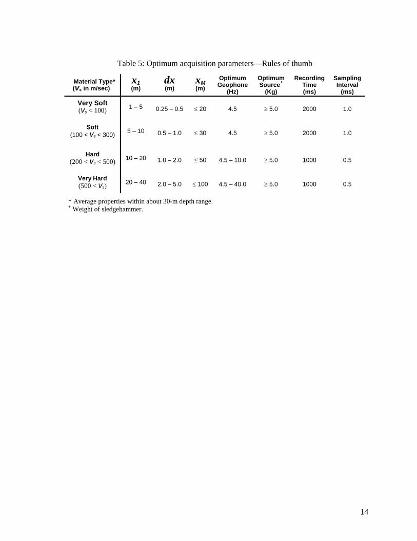
Table 5: Optimum acquisition parameters—Rules of thumb

Material Type* (vs in m/sec)

x1 (m)

dx (m)

xM (m)

Optimum Geophone

(Hz)

Optimum Source+

(Kg)

Recording Time (ms)

Sampling Interval

(ms)

Very Soft (vs < 100) 1 – 5 0.25 – 0.5 ≤ 20 4.5 ≥ 5.0 2000 1.0

Soft (100 < vs < 300) 5 – 10 0.5 – 1.0 ≤ 30 4.5 ≥ 5.0 2000 1.0

Hard (200 < vs < 500) 10 – 20 1.0 – 2.0 ≤ 50 4.5 – 10.0 ≥ 5.0 1000 0.5

Very Hard (500 < vs) 20 – 40 2.0 – 5.0 ≤ 100 4.5 – 40.0 ≥ 5.0 1000 0.5

* Average properties within about 30-m depth range. + Weight of sledgehammer.

14

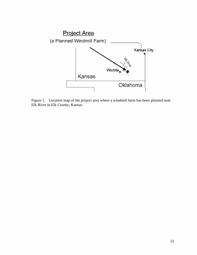
Figure 1. Location map of the project area where a windmill farm has been planned near Elk River in Elk County, Kansas.

15

16

(a)

(b) (c)

Figure 2. Illustration of optimum-offset window made by using a 48-channel walkaway shot record (a) acquired at T-012 site. The dispersion image obtained by processing traces covering (b) only nearer half offset range (1-24 channels) results in a M0 curve of superiorquality in comparison to (c) that from traces of the entire offset range.

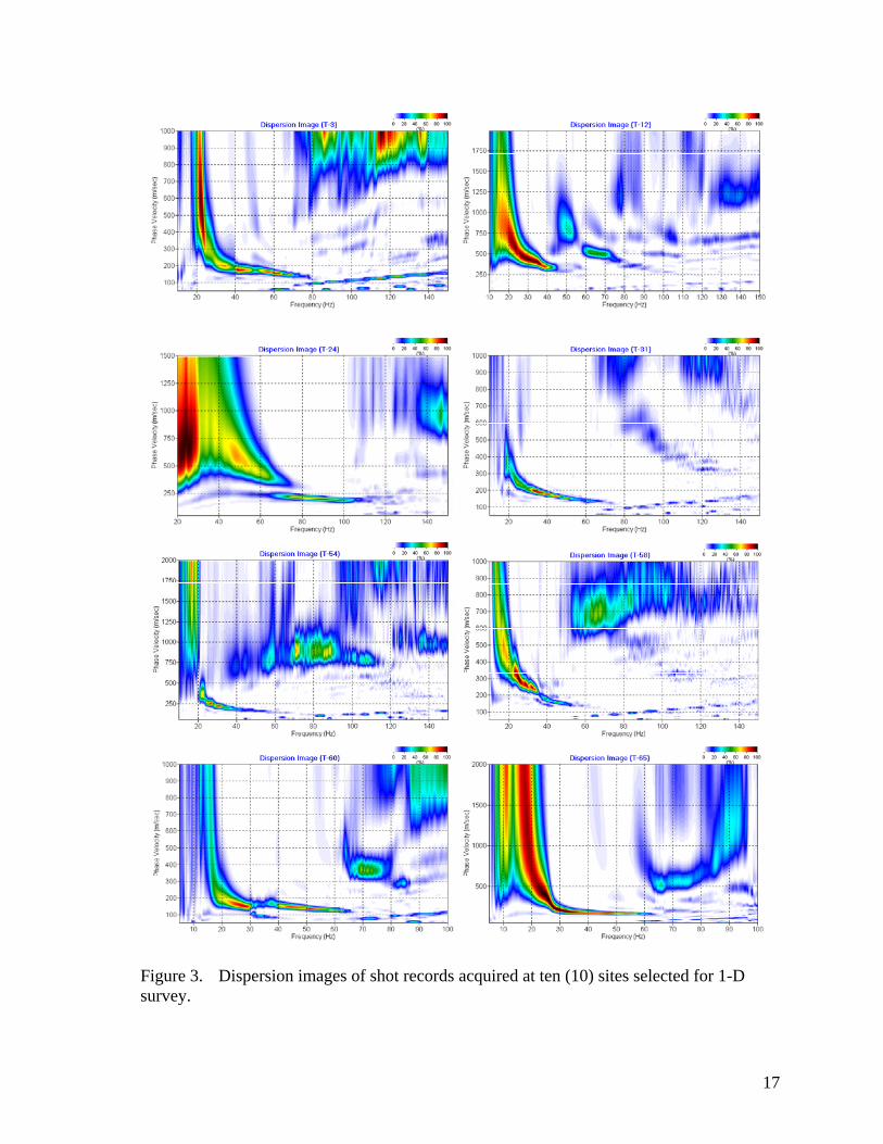
Figure 3. Dispersion images of shot records acquired at ten (10) sites selected for 1-D survey.

17

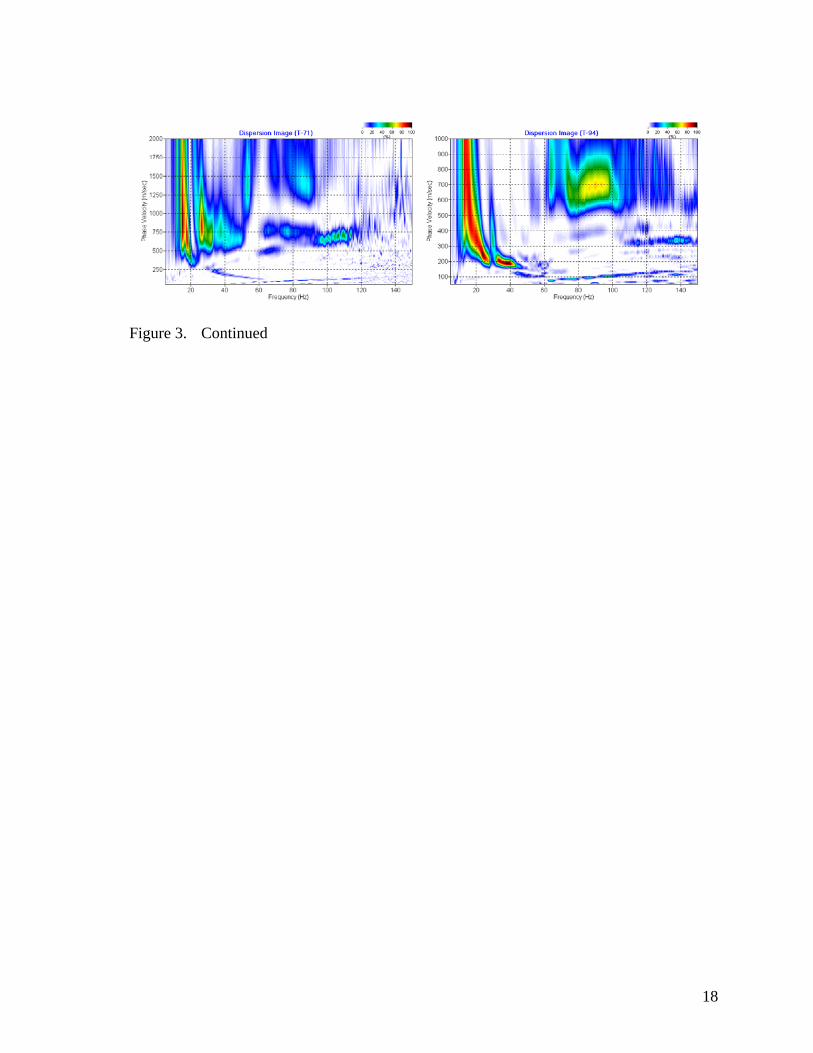
Figure 3. Continued

18

19

Figure 4. 1-D Vs profiles obtained from the MASW analysis for the ten 1-D sites.

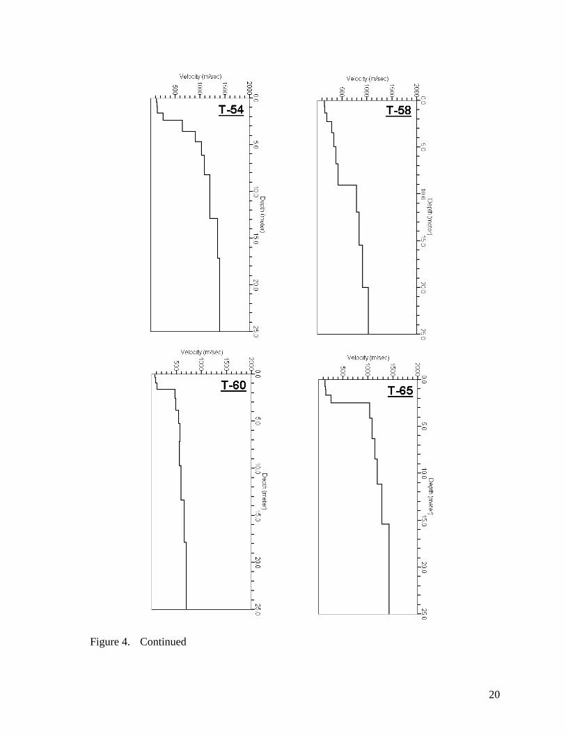
Figure 4. Continued

20

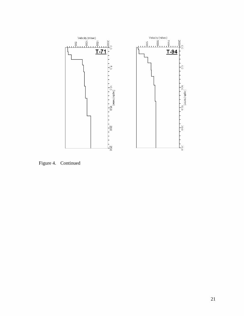
Figure 4. 1-D Vs profiles at ten (10) Elk River sites (continued)

Figure 4. Continued

21

22

Average Vs for Upper 5 m(Ten Selected Sites for 1-D Surveys, Elk County, Kansas)

0100200300400500600700800900

1000

3 12 24 31 54 58 60 65 71 94

Tower Number

Vs (m

/sec

)

Average Vs for Upper 10 m

(Ten Selected Sites for 1-D Surveys, Elk County, Kansas)

0100200300400500600700800900

1000

3 12 24 31 54 58 60 65 71 94

Tower Number

Vs (m

/sec

)

Average Vs for Upper 20 m

(Ten Selected Sites for 1-D Surveys, Elk County, Kansas)

0100200300400500600700800900

1000

3 12 24 31 54 58 60 65 71 94

Tower Number

Vs (m

/sec

)

Figure 5. Average Vs calculated for top 5 m (top), 10 m (middle), and 20 m (bottom) depth ranges at ten 1-D sites in Elk County, Kansas.

23

Four (4) seismic lines: Lines 1-4 Station spacing: 1.22 m (4 ft) Receivers: 4.5-Hz geophones Recording: 48-channel (2 of 24-channel Geometrics Geode) Source: 16-lb sledgehammer (3-impact stack) Recording: 1-sec recording time with 1-ms sampling interval Shot interval: 1 station Number of shots: 24 shots per line 2-D shear-velocity (Vs) imaging: all 4 lines Side scattering analysis (SSA): lines 2 and 4 Surface-wave imaging by attenuation (SIA): all 4 lines

Figure 6. A schematic showing the field logistics used for the 2-D surveys. Summary of acquisition parameters is listed on top.

24

Average Vs for Upper 5 m(Ten Selected Sites for 2-D Surveys, Elk County, Kansas)

0

100

200

300

400

500

600

700

800

900

1000

1 10 17 40 46 60 64 65 66 86

Tower Number

Vs (m

/sec

)

Average Vs for Upper 10 m(Ten Selected Sites for 2-D Surveys, Elk County, Kansas)

0

100

200

300

400

500

600

700

800

900

1000

1 10 17 40 46 60 64 65 66 86

Tower Number

Vs (m

/sec

)

Average Vs for Upper 20 m(Ten Selected Sites for 2-D Surveys, Elk County, Kansas)

0

100

200

300

400

500

600

700

800

900

1000

1 10 17 40 46 60 64 65 66 86

Tower Number

Vs (m

/sec

)

Figure 7. Average Vs calculated for top 5 m, 10 m, and 20 m depth ranges at ten 2-D sites in Elk County, Kansas. Average Vs values from N-S line (line 1) and E-W lines (lines 2-4) are also displayed.

25

Average Vs from N-S Line (Line 1)(Ten Selected Sites for 2-D Surveys, Elk County, Kansas)

0

100

200

300

400

500

600

700

800

900

1000

1 10 17 40 46 60 64 65 66 86

Tower Number

Vs (m

/sec

)

Average Vs from E-W Lines (Lines 2-4)

(Ten Selected Sites for 2-D Surveys, Elk County, Kansas)

0

100

200

300

400

500

600

700

800

900

1000

1 10 17 40 46 60 64 65 66 86

Tower Number

Vs (m

/sec

)

Figure 7. Continued

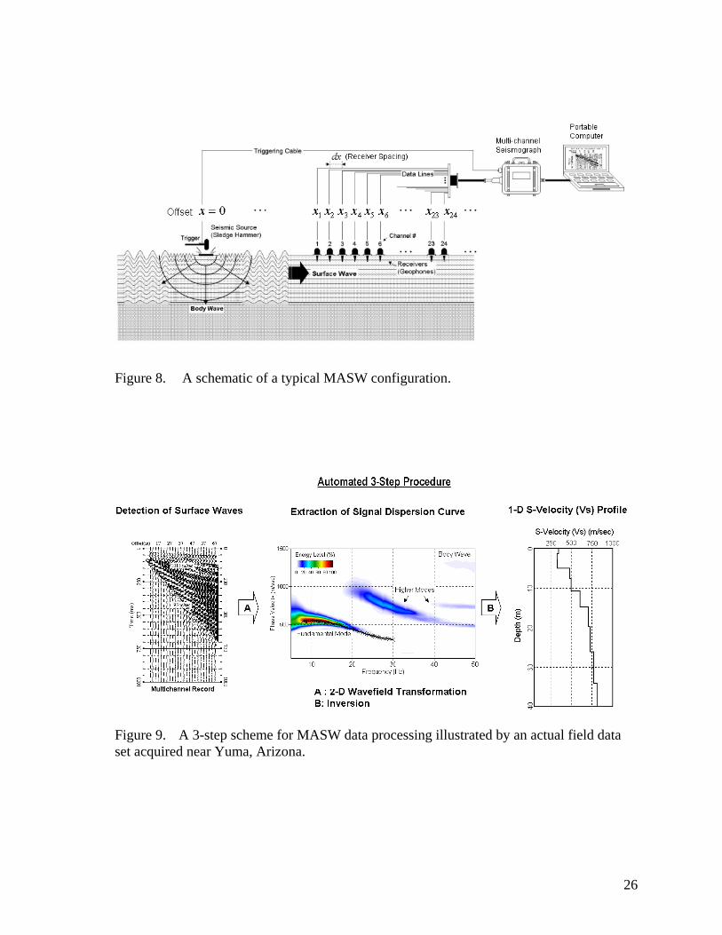
Figure 8. A schematic of a typical MASW configuration.

Figure 9. A 3-step scheme for MASW data processing illustrated by an actual field data set acquired near Yuma, Arizona.

26

27

Figure 10. Overall procedure to construct a 2-D Vs map from the MASW survey.

28

Figure 12. A plane-view schematic illustrating the scattered surface-wave generation that can be set off by a near-surface anomaly like a void.

Figure 11. A source-receiver configuration and an increment of the configuration.

29

Figure 14. An SSA map from modeling. Four (4) voids were modeled below the marked surface points with a spherical diameter (D) and a depth (Z) of (D=1m, Z=1m), (D=2m, Z=2m), (D=2m, Z=3m), and (D=1m, Z=3m) from top to bottom.

Figure 13. A fictitious grid net is used during the SSA processing in which each point (xv, yv) in the net is assumed as a possible scattering source of surface waves generated by a source at (xs, ys). Then, a receiver at (xr, yr) can record such scattered waves.

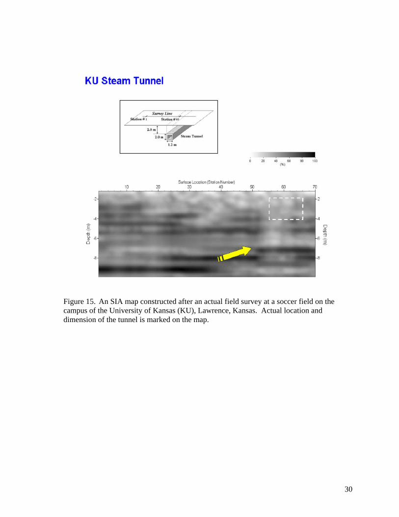
Figure 15. An SIA map constructed after an actual field survey at a soccer field on the campus of the University of Kansas (KU), Lawrence, Kansas. Actual location and dimension of the tunnel is marked on the map.

30