U. S. DEPARTMENT OF THE INTERIOR U. S. GEOLOGICAL SURVEY

Seismic Processing for Gas Hydrate Research Drill Site in the Mackenzie Delta, Canada

By

Myung W. Lee 1 and Warren F. Agena1

Open-File Report 98-593

This report is preliminary and has not been reviewed for conformity which U.S. Geological Survey editorial stands and stratigraphic nomenclature. Any use of trade, product, or firm names is for descriptive purposes only and does not imply endorsement by the U.S. Government.

*U.S. Geological Survey, Box 25046, Ms 939, Denver Federal Center, Denver, Colorado 80225

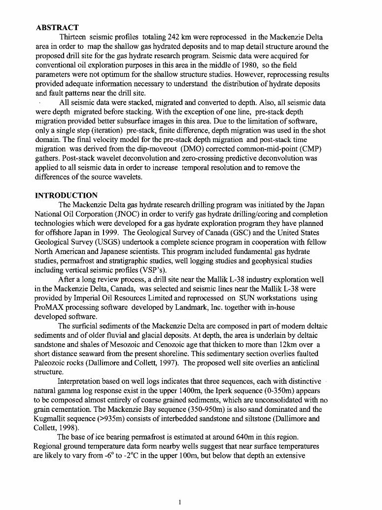
ABSTRACTThirteen seismic profiles totaling 242 km were reprocessed in the Mackenzie Delta

area in order to map the shallow gas hydrated deposits and to map detail structure around the proposed drill site for the gas hydrate research program. Seismic data were acquired for conventional oil exploration purposes in this area in the middle of 1980, so the field parameters were not optimum for the shallow structure studies. However, reprocessing results provided adequate information necessary to understand the distribution of hydrate deposits and fault patterns near the drill site.

All seismic data were stacked, migrated and converted to depth. Also, all seismic data were depth migrated before stacking. With the exception of one line, pre-stack depth migration provided better subsurface images in this area. Due to the limitation of software, only a single step (iteration) pre-stack, finite difference, depth migration was used in the shot domain. The final velocity model for the pre-stack depth migration and post-stack time migration was derived from the dip-moveout (DMO) corrected common-mid-point (CMP) gathers. Post-stack wavelet deconvolution and zero-crossing predictive deconvolution was applied to all seismic data in order to increase temporal resolution and to remove the differences of the source wavelets.

INTRODUCTIONThe Mackenzie Delta gas hydrate research drilling program was initiated by the Japan

National Oil Corporation (JNOC) in order to verify gas hydrate drilling/coring and completion technologies which were developed for a gas hydrate exploration program they have planned for offshore Japan in 1999. The Geological Survey of Canada (GSC) and the United States Geological Survey (USGS) undertook a complete science program in cooperation with fellow North American and Japanese scientists. This program included fundamental gas hydrate studies, permafrost and stratigraphic studies, well logging studies and geophysical studies including vertical seismic profiles (VSP's).

After a long review process, a drill site near the Mallik L-38 industry exploration well in the Mackenzie Delta, Canada, was selected and seismic lines near the Mallik L-38 were provided by Imperial Oil Resources Limited and reprocessed on SUN workstations using ProMAX processing software developed by Landmark, Inc. together with in-house developed software.

The surficial sediments of the Mackenzie Delta are composed in part of modern deltaic sediments and of older fluvial and glacial deposits. At depth, the area is underlain by deltaic sandstone and shales of Mesozoic and Cenozoic age that thicken to more than 12km over a short distance seaward from the present shoreline. This sedimentary section overlies faulted Paleozoic rocks (Dallimore and Collett, 1997). The proposed well site overlies an anticlinal structure.

Interpretation based on well logs indicates that three sequences, each with distinctive natural gamma log response exist in the upper 1400m, the Iperk sequence (0-350m) appears to be composed almost entirely of coarse grained sediments, which are unconsolidated with no grain cementation. The Mackenzie Bay sequence (350-950m) is also sand dominated and the Kugmallit sequence (>935m) consists of interbedded sandstone and siltstone (Dallimore and Collett, 1998).

The base of ice bearing permafrost is estimated at around 640m in this region. Regional ground temperature data form nearby wells suggest that near surface temperatures are likely to vary from -6° to -2°C in the upper 100m, but below that depth an extensive

isotherm section (close to -1°C) may occur. Ice bonding is expected to be quite variable throughout the sequence with possible taliks or non-ice bonding sections (Collett personal communication, 1998).

The wireline logs and mud gas log responses at Mallik L-38 indicate that there are 10 separate hydrated layers ranging in thickness from 3.4 m to 25.4 m and the total cumulative thickness of the hydrated layers are 111.4 m (Collett and Dalimore, 1997). The shallowest hydrate layer occurs at 819 m (Mackenzie Bay sequence) and the deepest hydrate layer occurs at 1091 m (Kugmallitt sequence). The existence of free gas under the hydrated layer was interpreted by Bily and Dick (1974) based on a spontaneous-potential well log response and a rapid pressure response during a production test. But Collett and Dallimore (1997) were not able to confirm the occurrence of free gas because of insufficient data.

The primary purpose of reprocessing was to image the continuity of the hydrate deposits near the proposed well site and to map the structural details around the drill site, particularly the fault patterns, so that the seismic profiles could be used to assist in spudding and drilling the gas hydrate research well. This report discusses the details of the processing steps.

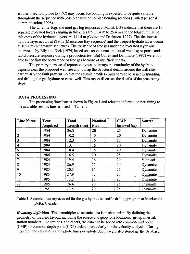
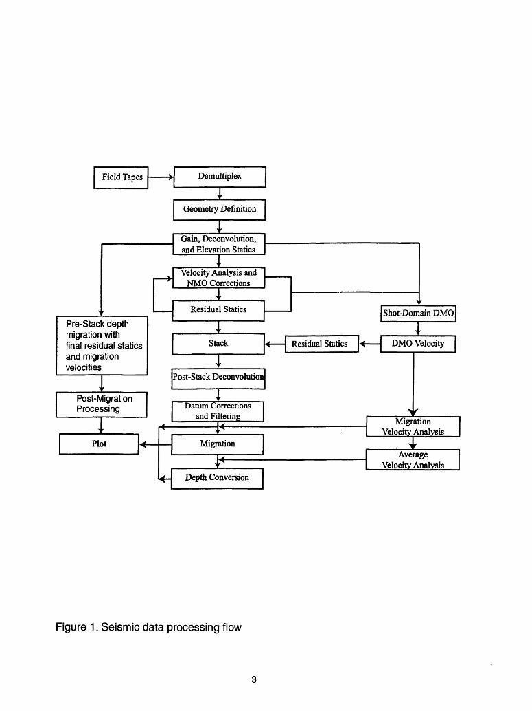
DATA PROCESSINGThe processing flowchart is shown in Figure 1 and relevant information pertaining to

the available seismic lines is listed in Table 1.

Line Name

12345678910111213

Year Acquired1984198419841984198419841984198419851985198519851985

Total Length (km)26.810.212.313.118.416.519.426.920.527.913.224.413.5

Nominal Fold20151515152016151532152020

CMPinterval (m)25201720202520202520252525

Source

DynamiteDynamiteDynamiteDynamiteDynamiteDynamiteVibroseisDynamiteDynamiteDynamiteDynamiteDynamiteDynamite

Table 1. Seismic lines reprocessed for the gas hydrate scientific drilling program at Mackenzie Delta, Canada.

Geometry definition- The demultiplexed seismic data is in shot order. By defining the geometry of the field layout, including the source and geophone locations, group interval, station numbers, live stations and others, the data can be sorted into common mid point (CMP) or common depth point (CDP) order, particularly for the velocity analysis. During this step, the elevations and uphole times or uphole depths were also stored in the database.

Field Tapes + Demultiplex

Pre-Stack depth migration with final residual statics and migration velocities

Post-Migration Processing

Geometry Definition

Gain, Deconvolution, and Elevation Statics

Velocity Analysis and NMO Corrections

Residual Statics Shot-Domain DMO

Stack 4 Residual Statics DMO Velocity

T|Post-Stack Deconvolutionl

Datum Corrections and Filtering

Plot Migration

Migration Velocity Analysis

Depth Conversion

Average Velocity Analysis^

Figure 1. Seismic data processing flow

The data were acquired using a split spread geometry with 120 receiver channels except for line 7, which used 96 receiver channels. The geophone group intervals varied between 34 to 50 m (Table 1) with a nominal interval of 50 m.

Gain, deconvolution and elevation statics. - Because our primary concerns in the reprocessing were to map continuity of hydrated layers and structural mapping, preserving relative amplitudes was not considered important. Therefore using an AGC with a 300 ms window is acceptable for the gain function.

In order to increase the temporal resolution, a spectral whitening method (Lee, 1986) was applied instead of conventional spiking deconvolution. Tests indicated that the spectral whitening technique preserved the continuity of shallow reflections better than the spiking deconvolution technique. As mentioned previously, one of the main concerns was to map the continuity of shallow hydrate layers, so we opted to use spectral whitening method for all the seismic lines for this reprocessing.

Elevations in this area are relatively flat, so choosing a floating or a flat datum for the processing was immaterial. For convenience, we used a floating datum by smoothing the actual elevations over 200 CMP's. Using this floating datum or normal moveout (NMO) datum, elevation statics were computed and applied to individual traces. This floating datum was corrected to a final flat datum (sea level) prior to migration.

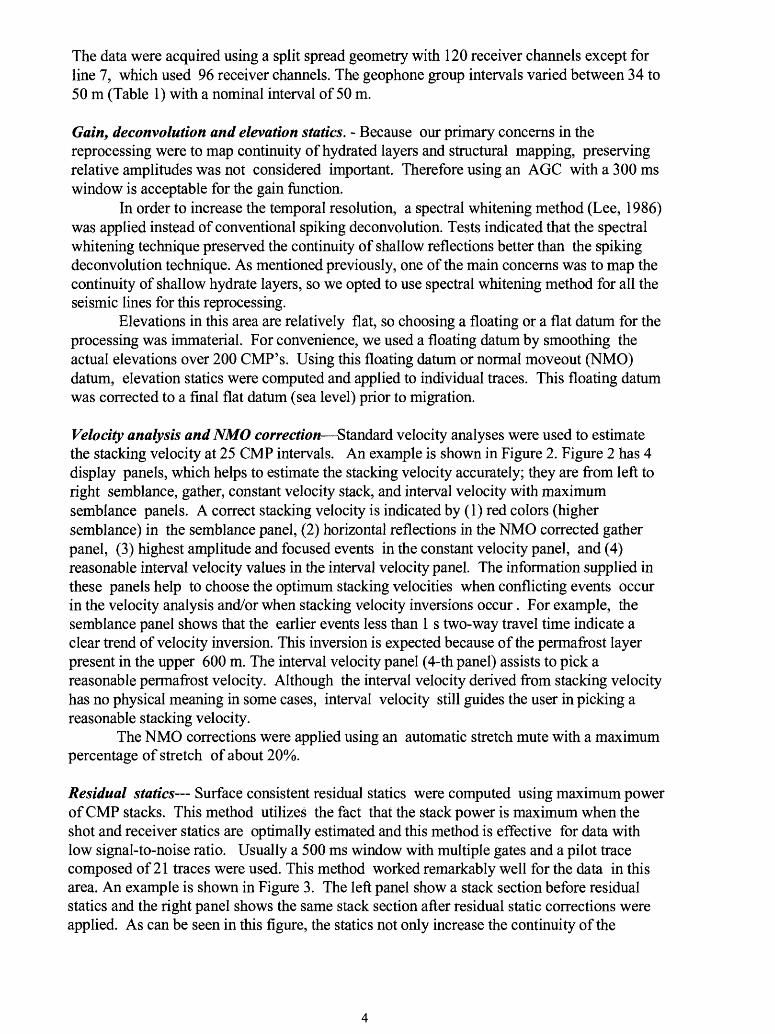
Velocity analysis and NMO correction Standard velocity analyses were used to estimate the stacking velocity at 25 CMP intervals. An example is shown in Figure 2. Figure 2 has 4 display panels, which helps to estimate the stacking velocity accurately; they are from left to right semblance, gather, constant velocity stack, and interval velocity with maximum semblance panels. A correct stacking velocity is indicated by (1) red colors (higher semblance) in the semblance panel, (2) horizontal reflections in the NMO corrected gather panel, (3) highest amplitude and focused events in the constant velocity panel, and (4) reasonable interval velocity values in the interval velocity panel. The information supplied in these panels help to choose the optimum stacking velocities when conflicting events occur in the velocity analysis and/or when stacking velocity inversions occur. For example, the semblance panel shows that the earlier events less than 1 s two-way travel time indicate a clear trend of velocity inversion. This inversion is expected because of the permafrost layer present in the upper 600 m. The interval velocity panel (4-th panel) assists to pick a reasonable permafrost velocity. Although the interval velocity derived from stacking velocity has no physical meaning in some cases, interval velocity still guides the user in picking a reasonable stacking velocity.

The NMO corrections were applied using an automatic stretch mute with a maximum percentage of stretch of about 20%.

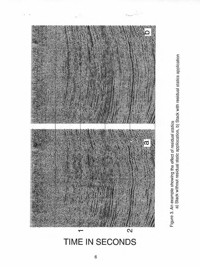
Residual statics Surface consistent residual statics were computed using maximum power of CMP stacks. This method utilizes the fact that the stack power is maximum when the shot and receiver statics are optimally estimated and this method is effective for data with low signal-to-noise ratio. Usually a 500 ms window with multiple gates and a pilot trace composed of 21 traces were used. This method worked remarkably well for the data in this area. An example is shown in Figure 3. The left panel show a stack section before residual statics and the right panel shows the same stack section after residual static corrections were applied. As can be seen in this figure, the statics not only increase the continuity of the

Figu

re 2

. An

exam

ple

of v

eloc

ity a

naly

sis.

Fro

m le

ft to

rig

ht,

sem

blan

ce v

eloc

ity p

anel

, CM

P g

athe

rpa

nel,

cons

tant

vel

ocity

sta

ck p

anel

, in

terv

al v

eloc

ity (b

lack

line

), an

d se

mbl

ance

(co

lor)

pane

l.

c g " * <OJ .0"a. o.coCOo

" * <CO 4 I CO

"co

'coo

.oCO

co COO x-v

CO *-; 3 CO

II0) Q.

*- o o *=

CD CO

C 0)"^ -O 13 c oCO ^o-|Q. >

E ^^ ^>S ^s0) CO

CO

13 O)

TIME IN SECONDS

reflections, but also increase temporal resolution because the reflected events after static corrections are better focused in the CMP domain.

Velocity analysis and residual static computations are iterative processes. Until a satisfactory stack section is obtained or there are no further significant changes in the stacking velocity, the process iterates as shown in Figure 1. Usually a minimum of 2 iterations were adequate, but sometimes 3 iterations of static and velocity analysis were

required.

Stack The CMP gathers were stacked with the optimum velocities and statics . We tested a variety of stack methods using a median (instead of summing the samples, takes the median of the samples at each trace time), mean (sums the sample values and divides by a square root of the number of samples), and weighted mean (before summing, the samples are multiplied by weights; e.g., weights proportional to the offsets to reduce the multiple energy). Because the mean method usually worked effectively, all data were stacked using mean method.

Shot-domain DMO The stacking velocity or NMO velocity depends on the dip of the reflector. It is well known that the conventional stacking method cannot stack both a flat and dipping layer occurring simultaneously because of the dip dependence of the stacking velocity. The dip moveout (DMO) process is a method to improve the stack quality by compensating for the dip effect in the NMO equation.

The arrival time for a single reflector is given by the following equation (Levin, 1971).

T2 (x) = r2 (0) + jt 2 cos2 (0)/F 2 - r2 (0) + * 2 /Vn2mo Equation (1).

where T is the two-way travel time from a source to a receiver, x is an offset distance, 0 is a dip angle of a reflector, V is the medium velocity, and Vnmo is a normal moveout velocity or stacking velocity. In a multi-layered case, the right side of Equation (1) is approximately correct and the normal moveout velocity Vnmo becomes the root mean square velocity (Vrms). Because the stacking velocity (or Vnmo) analysis approximates the right side of Equation (1) with hyperbolas, Vnmo contains the dip effect.

To see the effect of dip and interval velocity on the moveout time, Equation (1) is changed into the following formula (Yilmaz, 1987).

T2 (x) = T2 (0) + x2 IV 2 - x 2 sin2 (6) IV2 Equation (2).

In this equation, the first part of moveout (the second term, x 2 1V 2 ) is called zero-dip normal moveout and the second part (the third term) is associated with dip moveout (DMO). DMO processing is a scheme to compensate for the dip dependence of the NMO equation and makes the NMO equation independent of the dip angle. As indicated in the flow chart, the velocity and the statics for the regular stack process were the inputs to the DMO processing. DMO velocities were estimated using the same method as mentioned above.

One advantage of DMO processing is the improvement of velocity analysis, because it provides velocities which are more appropriate for use in migration (Deregowski and Rocca, 1981). Therefore all of the data have been processed using DMO in the shot-domain in order to derive a migration velocity model, which is used for the post-stack migration, post- stack depth conversion and pre-stack depth migration.

00

m m

o

O z D

Figu

re 4

. An

exam

ple

show

ing

the

effe

ct o

f pos

t-sta

ck w

avel

et d

econ

volu

tion.

a)

stac

k w

ith p

ost-s

tack

sec

ond-

zero

cr

ossi

ng d

econ

volu

tion.

b)

Sta

ck w

ith p

ost-s

tack

sec

ond-

zero

cro

ssin

g de

conv

olut

ion

and

mat

ched

filte

ring,

c)

Sta

ck w

ith p

ost-s

tack

sec

on-z

ero

cros

sing

and

wav

elet

dec

onvo

lutio

n .

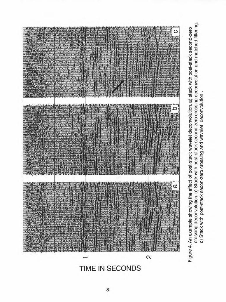
Post-stack deconvolution--- Because of the different sources used (dynamite and Vibroseis) and the reverberatory energy present in the stacked section, a post-stack deconvolution was applied to all stacked data in order to correct for the differences in source type and increase temporal resolution. A 1000 ms AGC was applied before the post-stack deconvolution, which included a second-zero crossing and wavelet deconvolution. Second-zero crossing deconvolution is a type of predictive deconvolution where the prediction distance is the second-zero crossing of the auto-correlation of the trace. A single window with 140 ms operator length was used.

In wavelet processing, a variable norm deconvolution method by Gray (1979) was applied in the reprocessing. About 100 random windows (window length is about 18 ms) were selected between about 200 and 1000 ms in the stacked data and wavelets were estimated using different norms, window lengths, and design area. The deconvolved outputs were compared visually and optimum parameters were chosen. A single deconvolution operator was derived from the optimum parameters and applied to the whole line.

Figure 4 shows an example of this post-stack process. Figure 4a shows the final stacked section with the application of the post-stack second-zero crossing deconvolution, Figure 4b shows the result after the application of a matched filtering as well as the post-stack second- zero crossing deconvolution, and Figure 4c shows the result after the application of the post- stack second-zero crossing and wavelet deconvloution. A matched filtering is crosscorrelating seismic section with the estimated wavelet (Claerbout, 1992). If the extracted wavelet is close to the actual wavelet present in the seismic section, the output after the matched filtering increases the signal-to-noise ratio of the section. This happens because the matched filtering enhances the spectral component of the wavelet and reduces the spectral component of uncorrelated random noise. In comparing Figures 4a and 4b, it is clear that reflected events in the upper 500 ms are imaged better in Figure 4b. Thus it is concluded that the estimated wavelet is close to the actual wavelet present in the seismic data in this case. Figure 4c indicates that the wavelet deconvolution improves temporal resolution as well as correcting the phase of wavelet, which is clearly demonstrated in the area indicated by the arrow.

Determining the validity of the wavelet deconvolution (or equivalently wavelet estimation) is difficult without sonic logs or other independent measurement of wavelets, and there is a subjective component in estimating the wavelet. However, the result of the matched filtering provides an additional constraint in choosing the optimum wavelet

Datum Correction and Filtering Prior to migration, all stacked data were corrected to a final flat datum (sea level) by using simple static shifts. A band pass filter with 8-10-68-92 Hz pass band was also applied.

Migration - The stacked data were migrated using Stolt's wave-number frequency domain migration method using migration velocity models derived from the DMO stacking velocities, which will be described later in the section entitled " Derivation of Velocities".

Depth Conversion The migrated data were depth-converted using average velocities (See Derivation of Velocities). Usually for depth conversion, well data or vertical seismic profile (VSP) data are used to constrain the average velocity. Because the sonic data at Mallik L- 38 are severely degraded (clipped in the hydrated interval), the average velocities are derived solely from the DMO velocities.

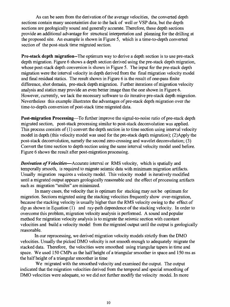
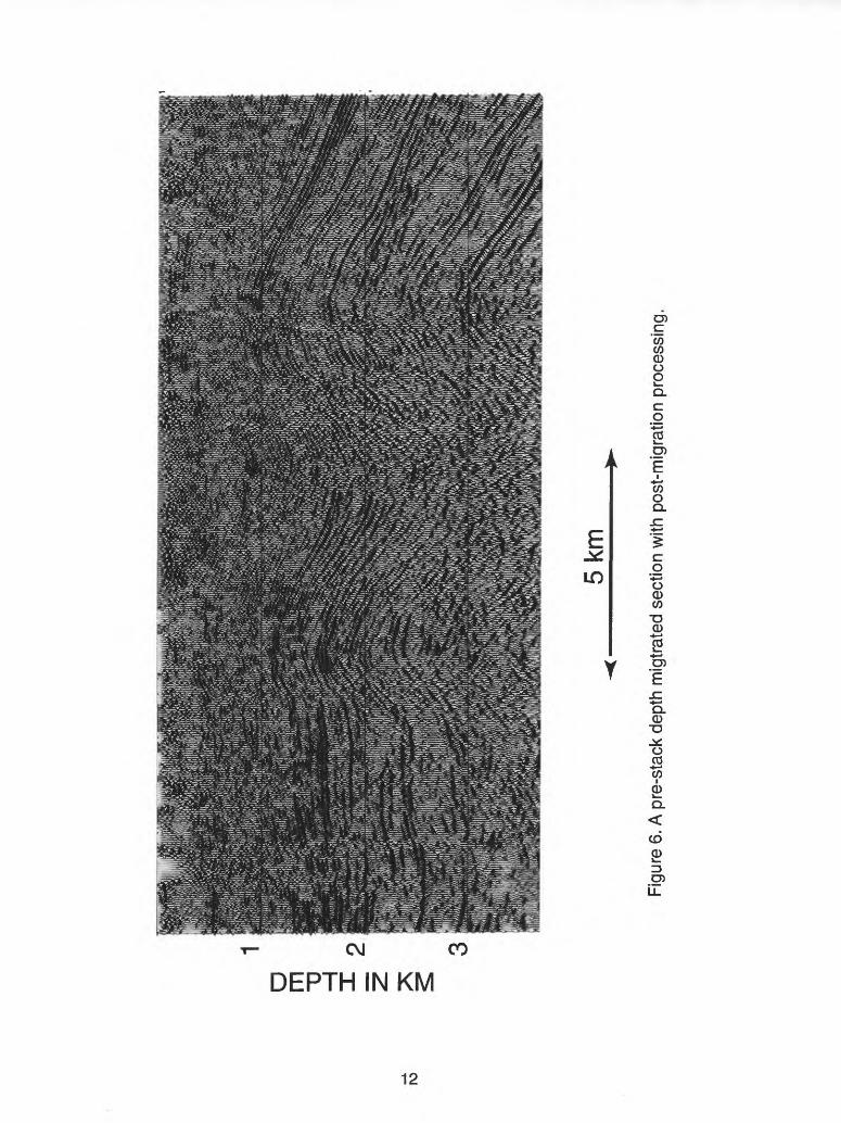
As can be seen from the derivation of the average velocities, the converted depth sections contain many uncertainties due to the lack of well or VSP data, but the depth sections are geologically sound and generally accurate. Therefore, these depth sections provide an additional advantage for structural interpretation and planning for the drilling at the proposed site. An example is shown in Figure 5, which is a time-to-depth converted section of the post-stack time migrated section.

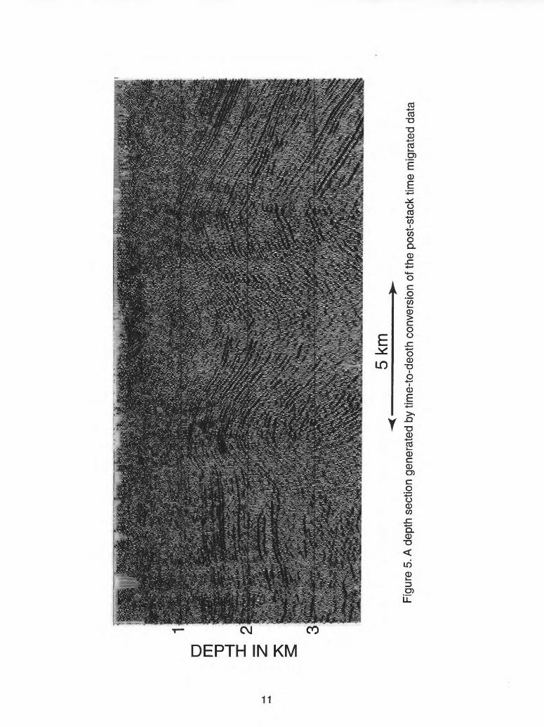
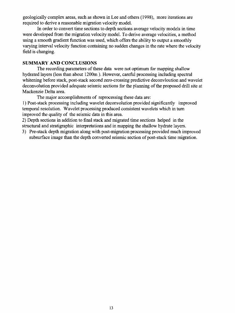
Pre-stack depth migration The optimum way to derive a depth section is to use pre-stack depth migration. Figure 6 shows a depth section derived using the pre-stack depth migration, whose post-stack depth conversion is shown in Figure 5. The input for the pre-stack depth migration were the interval velocity in depth derived from the final migration velocity model and final residual statics. The result shown in Figure 6 is the result of one-pass finite difference, shot domain, pre-stack depth migration. Further iterations of migration velocity analysis and statics may provide an even better image than the one shown in Figure 6. However, currently, we lack the necessary software to do iterative pre-stack depth migration. Nevertheless this example illustrates the advantages of pre-stack depth migration over the time-to-depth conversion of post-stack time migrated data.

Post-migration Processing To further improve the signal-to-noise ratio of pre-stack depth migrated section, post-stack processing similar to post-stack deconvolution was applied. This process consists of (1) convert the depth section in to time section using interval velocity model in depth (this velocity model was used for the pre-stack depth migration); (2)Apply the post-stack deconvolution, namely the second zero-crossing and wavelet deconvolution; (3) Convert the time section to depth section using the same interval velocity model used before. Figure 6 shows the result after post-migration processing.

Derivation of Velocities Accurate interval or RMS velocity, which is spatially and temporally smooth, is required to migrate seismic data with minimum migration artifacts. Usually migration requires a velocity model. This velocity model is iteratively modified until a migrated output appears geologically reasonable and the effect of processing artifacts such as migration "smiles" are minimized.

In many cases, the velocity that is optimum for stacking may not be optimum for migration. Sections migrated using the stacking velocities frequently show over-migration, because the stacking velocity is usually higher than the RMS velocity owing to the effect of dip as shown in Equation (1) and ray-path dependence of the stacking velocity. In order to overcome this problem, migration velocity analysis is performed. A sound and popular method for migration velocity analysis is to migrate the seismic section with constant velocities and build a velocity model from the migrated output until the output is geologically reasonable.

In our reprocessing, we derived migration velocity models strictly from the DMO velocities. Usually the picked DMO velocity is not smooth enough to adequately migrate the stacked data. Therefore, the velocities were smoothed using triangular tapers in time and space. We used 150 CMPs as the half height of a triangular smoother in space and 150 ms as the half height of a triangular smoother in time

We migrated with the smoothed velocity and examined the output. The output indicated that the migration velocities derived from the temporal and special smoothing of DMO velocities were adequate, so we did not further modify the velocity model. In more

10

o

m

TJ

5 km

Figu

re 5

. A d

epth

sec

tion

gene

rate

d by

tim

e-to

-deo

th c

onve

rsio

n of

the

post

-sta

ck ti

me

mig

rate

d da

ta

D m "D

5 km

Figu

re 6

. A p

re-s

tack

dep

th m

igtra

ted

sect

ion

with

pos

t-mig

ratio

n pr

oces

sing

.

geologically complex areas, such as shown in Lee and others (1998), more iterations are required to derive a reasonable migration velocity model.

In order to convert time sections to depth sections average velocity models in time were developed from the migration velocity model. To derive average velocities, a method using a smooth gradient function was used, which offers the ability to output a smoothly varying interval velocity function containing no sudden changes in the rate where the velocity field is changing.

SUMMARY AND CONCLUSIONSThe recording parameters of these data were not optimum for mapping shallow

hydrated layers (less than about 1200m). However, careful processing including spectral whitening before stack, post-stack second zero-crossing predictive deconvloution and wavelet deconvolution provided adequate seismic sections for the planning of the proposed drill site at Mackenzie Delta area.

The major accomplishments of reprocessing these data are:1) Post-stack processing including wavelet deconvolution provided significantly improved temporal resolution. Wavelet processing produced consistent wavelets which in turn improved the quality of the seismic data in this area.2) Depth sections in addition to final stack and migrated time sections helped in the structural and stratigraphic interpretations and in mapping the shallow hydrate layers.3) Pre-stack depth migration along with post-migration processing provided much improved

subsurface image than the depth converted seismic section of post-stack time migration.

13

REFERENCES

Bily, C. and Dick, J.W.L., 1974, Natural occurring gas hydrates in the Mackenzie Delta, Northwest Territories: Bulletin of Canadian Petroleum Geology, v. 22, no. 3, p. 340-352.

Claerbout, J.F., 1992, Earth sounding analysis: Blackwell Scientific Publications, Boston, 304 p.

Collett, T.S. and Dallimore, S.R., 1997, Quantitative assessment of gas hydrates in the Mallik L-38 well, Mackenzie Delta, N.W.T: Proceedings of the 7th International Conference on Permafrost, 8 p.

Dallimore, S.R. and Collett, T.S., 1997, Gas hydrate associated with deep permafrost in the Mackenzie Delta, N.W.T., Canada: Regional overview: Proceedings of the 7th International Conference on Permafrost, 10 p.

Deregowski, S. and Rocca, F., 1981, Geometrical optics and wave theory for constant-offset sections in layered media, Geophysical Prospecting, v. 29, p. 374-387.

Gray, W.C., 1979, Variable norm deconvolution: Palo Alto, CA, Stanford University Ph.D. Thesis, p. 101.

Lee, M.W., 1986, Spectral whitening in the frequency domain: U.S. Geological Survey Open File Report 86-553, 15 p.

Lee, M.W., Agena, W.F., Grow, J.A., and Miller, J.J., 1998, Seismic Processing and Velocity Analysis in The Oil and Gas Resource Potential of the 1002 Area, Arctic National Wildlife Refuge, Alaska, by ANWR Assessment Team, U. S. Geological Survey Open File Report 98-34, 29 p.

Levin, F.K, 1971, Apparent velocity from dipping interface reflections: Geophysics, v. 36, p. 510-516.

Yilmaz, Ozdogan, 1987, Seismic data processing: Society of Exploration of geophysics- Investigations in Geophysics, V.2,, 526 p.

14