SEISMIC RISK OF INDUSTRIAL PLANTS: ASSESSMENT …users.ntua.gr/divamva/docs/StuMS/Danesi_MSThesis2015.pdf · The dissertation entitled “Seismic Risk of Industrial Plants: Assessment

SEISMIC RISK OF INDUSTRIAL PLANTS:

ASSESSMENT OF A PETROCHEMICAL

PIPERACK USING INCREMENTAL

DYNAMIC ANALYSIS

A Dissertation Submitted in Partial Fulfilment of the Requirements

for the Master Degree in

Earthquake Engineering

By

Rodolfo José Danesi

Supervisors: Prof. Paolo Bazzurro & Prof. Dimitrios Vamvatsikos

February, 2015

Istituto Universitario di Studi Superiori di Pavia

Università degli Studi di Pavia

The dissertation entitled “Seismic Risk of Industrial Plants: Assessment of a Petrochemical Piperack using Incremental Dynamic Analysis”, by Rodolfo José Danesi, has been approved in partial fulfilment of the requirements for the Master Degree in Earthquake Engineering.

Prof. Dr. Paolo Bazzurro …… … ………

Prof. Dr. Dimitrios Vamvatsikos ………… … ……

Abstract

ABSTRACT Past earthquakes have demonstrated that industrial facilities such as petrochemical refineries can become largely damaged from the effects of strong ground motions. While much information on seismic assessment is related to conventional buildings, a lack of information is apparent with respect to most industrial infrastructure. As a matter of fact, most of the structures found in such facilities are complex by the nature of the operating process. This study evaluates the seismic performance of a modern piperack, which is representative of a typical typology present in refineries. A numerical 3D model built in the OpenSees platform is used to examine the response of the steel structure and the piping system attached to the mechanical equipment. The analysis method selected is incremental dynamic analysis (IDA), which involves multiple nonlinear time history analysis under a suite of ground motion records. The resultant set of IDA curves are in turn used to generate analytical fragility functions for the piping system in order to quantify the seismic risk of product leakage. It is envisioned that such tools can constitute a valid element for risk reduction decision making. Keywords: industrial facilities; piperack; piping system; incremental dynamic analysis; fragility functions; leakage

i

Acknowledgements

ACKNOWLEDGEMENTS Following a chronological order, I would first like to thank my referees, Prof. Francisco Crisafully, Prof. Bibiana Luccioni and Prof. Enrique Galindez, who played an important role by writing the letters of reference for my scholarship application. Thanks to the MEEES programme for awarding me the scholarship and giving me the financial support to improve my education in Europe. Destiny did not allow me to do this Master course in 2008 and I am now happy to have been able to complete it. Special thanks to my supervisors, Prof. Paolo Bazzurro and Prof. Dimitrios Vamvatsikos. Paolo thank you very much because, although being part time at the University and loaded with tons of work, you not only accepted my supervisor request but also contacted Dimitrios to help in the cause. Thanks Dimitrios for your time and guidance, for all your quick and helpful replies flavoured with your particular sense of humour. And, in name of the community, thanks for sharing you magic through your papers and Matlab-OpenSees routines. Last but not least, I would like to thank to all the persons who kindly helped me and had to tolerate me in my non happy, stressed days: family, Gringa, friends and classmates.

ii

Index

TABLE OF CONTENTS

Page

ABSTRACT ............................................................................................................................................ i

ACKNOWLEDGEMENTS .................................................................................................................... ii

TABLE OF CONTENTS ...................................................................................................................... iii

LIST OF FIGURES ................................................................................................................................ v

LIST OF TABLES ................................................................................................................................ vii

1 INTRODUCTION ............................................................................................................................. 1

1.1 Motivation .................................................................................................................................. 1

1.2 Objectives .................................................................................................................................. 2

1.3 Outline of the Thesis .................................................................................................................. 2

2 DAMAGE FROM PAST EARTHQUAKES IN MAJOR INDUSTRIAL FACILITIES ................. 3

2.1 Introduction ................................................................................................................................ 3

2.2 Earthquakes reported and performance of components ............................................................. 3

2.3 Damage summary ...................................................................................................................... 7

3 DESCRIPTION OF THE CASE STUDY ......................................................................................... 8

3.1 Description of the analytical model ......................................................................................... 10

3.1.1 Materials ........................................................................................................................ 11

3.1.2 Modelling of the steel structure ..................................................................................... 12

3.1.3 Modelling of the air coolers equipment ......................................................................... 13

3.1.4 Modelling of the piping system ..................................................................................... 14

3.1.5 Modelling of masses ...................................................................................................... 17

3.2 Modal analysis: Eigenvalues .................................................................................................... 17

4 ASSESSMENT OF THE CASE STUDY USING INCREMENTAL DYNAMIC ANALYSIS .... 20

4.1 Introduction .............................................................................................................................. 20

iii

Index

4.2 Incremental Dynamic Analysis (IDA) ..................................................................................... 20

4.2.1 Description of the method .............................................................................................. 20

4.2.2 Definition of the main variables: IM and EDP(s) .......................................................... 21

4.2.3 Suite of ground motions: ATC-63 ................................................................................. 22

4.2.4 Performing IDA ............................................................................................................. 22

4.2.5 Postprocessing IDA ....................................................................................................... 23

4.2.6 SPO vs IDA.................................................................................................................... 24

4.3 Seismic vulnerability of the AC piping system ....................................................................... 29

4.3.1 Definition of Damage State (DS) ................................................................................... 29

4.3.2 Rotational capacity of fittings at first leakage (EDPcap) ................................................. 30

4.3.3 Piping fittings monitored for fragility functions ............................................................ 30

4.3.4 Estimation of fragility functions using fitting IDA curves ............................................ 31

4.3.5 Visualizing the piping DS on piperack IDA curves ....................................................... 34

5 CONCLUSIONS ............................................................................................................................. 35

5.1 Summary .................................................................................................................................. 35

5.2 Future work .............................................................................................................................. 36

REFERENCES ..................................................................................................................................... 37

iv

Index

LIST OF FIGURES

Page

Figure 2.1. Damage observed in pipes ..................................................................................................... 5

Figure 2.2. Shear failure of anchor bolt [Roche et al., 1995] (left and middle); ..................................... 6

Figure 2.3. Damage to AC support structure [Stepp et al., 1990] ........................................................... 6

Figure 3.1. Key plan Alkylation Unit ...................................................................................................... 8

Figure 3.2. Main Piperack south view ..................................................................................................... 8

Figure 3.3. Typical transverse moment frame ......................................................................................... 9

Figure 3.4. Longitudinal braced frame .................................................................................................. 10

Figure 3.5. Roof plan view .................................................................................................................... 10

Figure 3.6. Perspective view of Piperack model .................................................................................... 11

Figure 3.7. Modelling of braces ............................................................................................................. 13

Figure 3.8. Air coolers operating system ............................................................................................... 13

Figure 3.9. Air coolers model ................................................................................................................ 14

Figure 3.10. 3D view of inlet and outlet header piping ......................................................................... 15

Figure 3.11. Modelling of fittings .......................................................................................................... 15

Figure 3.12. Flexibility Factor: ASME B31.3 Table D300 (left) & Air Coolers piping fittings (right) 16

Figure 3.13. Header support structure.................................................................................................... 17

Figure 3.14. Modal shape in transverse direction T1=0.881sec ............................................................ 18

Figure 3.15. Modal shape in longitudinal direction T7=0.468sec ......................................................... 19

Figure 4.1. Twenty-two IDA curves for the maximum interstory drift in the transverse direction

(Moment Frames) .......................................................................................................................... 25

Figure 4.2. The corresponding 16, 50 and 84% fractile IDA curves of Figure 4.1 ............................... 25

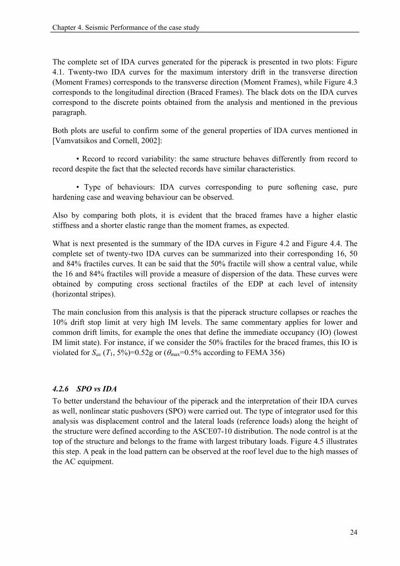
Figure 4.3. Twenty-two IDA curves for the maximum interstory drift in the longitudinal direction

(Braced Frames) ............................................................................................................................ 26

Figure 4.4. The corresponding 16, 50 and 84% fractile IDA curves of Figure 4.3 ............................... 26

Figure 4.5. SPO load pattern for both directions ................................................................................... 27

v

Index

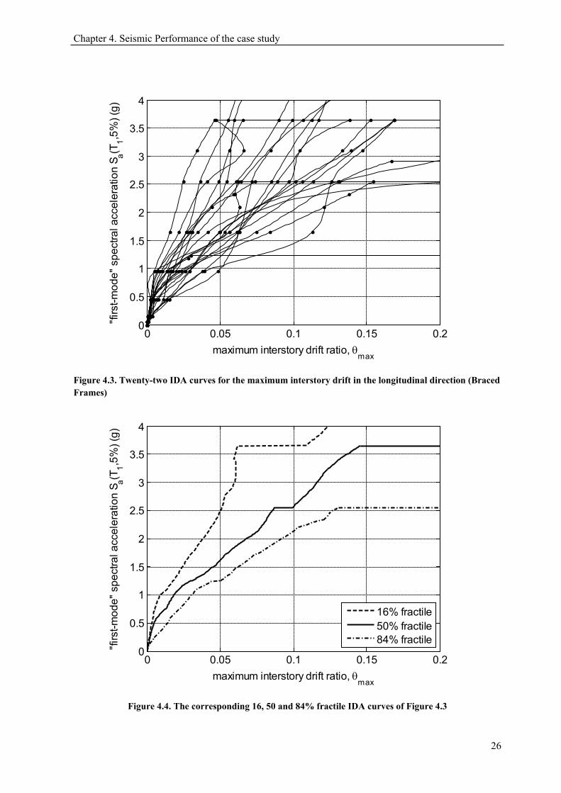
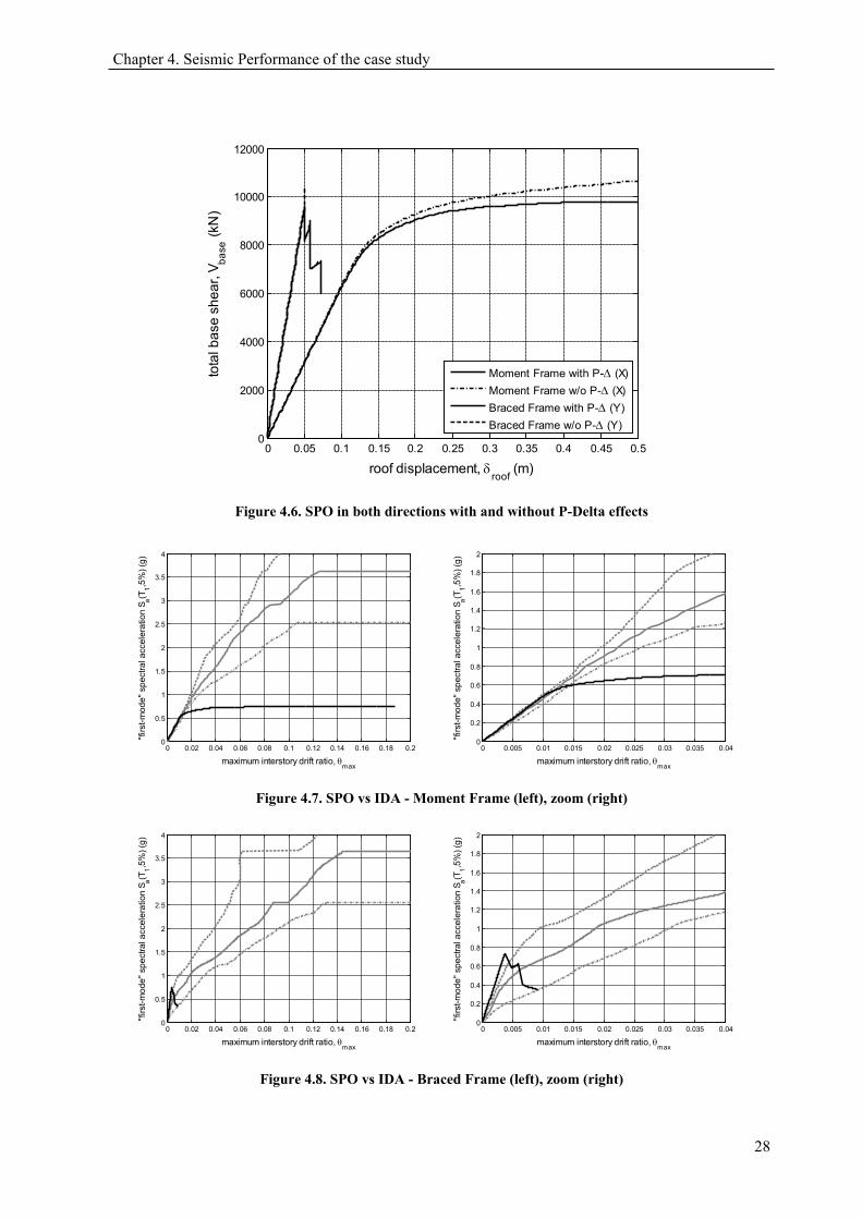
Figure 4.6. SPO in both directions with and without P-Delta effects .................................................... 28

Figure 4.7. SPO vs IDA - Moment Frame (left), zoom (right) .............................................................. 28

Figure 4.8. SPO vs IDA - Braced Frame (left), zoom (right) ................................................................ 28

Figure 4.9. Piping system monitored for fragility functions .................................................................. 30

Figure 4.10. Examples of IDA curves obtained for piping fittings: 4”(top); 6”(middle); 8”(bottom) ... 31

Figure 4.11. Fragility functions for 4" pipe fitting ................................................................................ 33

Figure 4.12. Fragility function 6" pipe fitting ........................................................................................ 33

Figure 4.13. Fragility function 8" pipe fitting ........................................................................................ 33

Figure 4.14. Fragility function regardless pipe diameter ....................................................................... 34

Figure 4.15. Leakage point on piperack IDA curves: Moment frame (left) ; Braced frame (right) ...... 34

vi

Index

LIST OF TABLES

Page

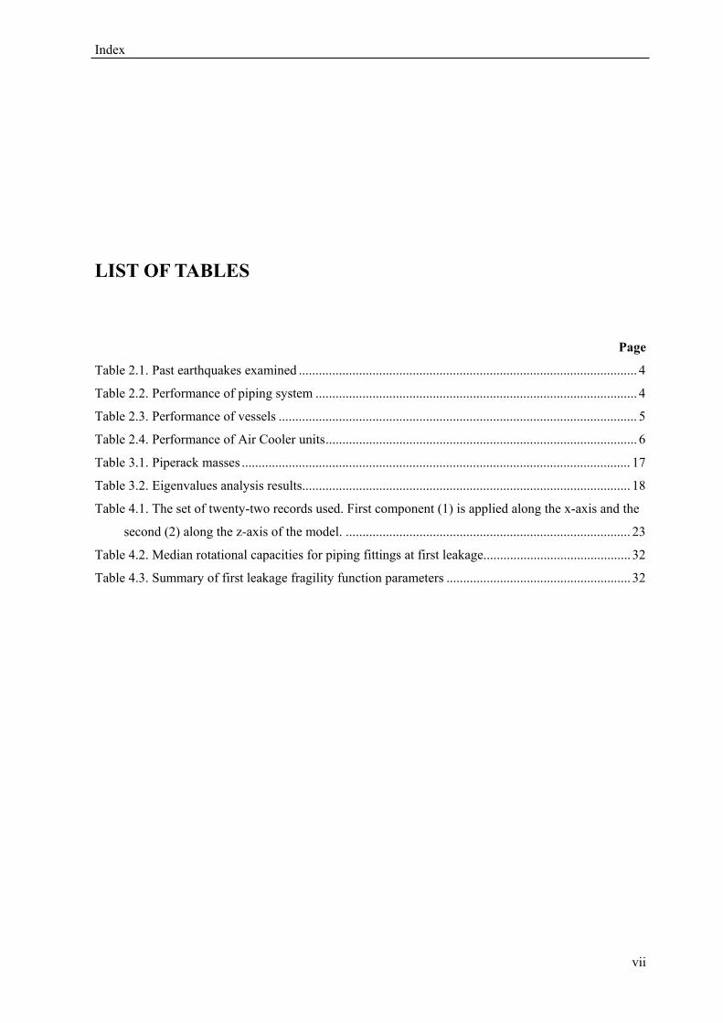
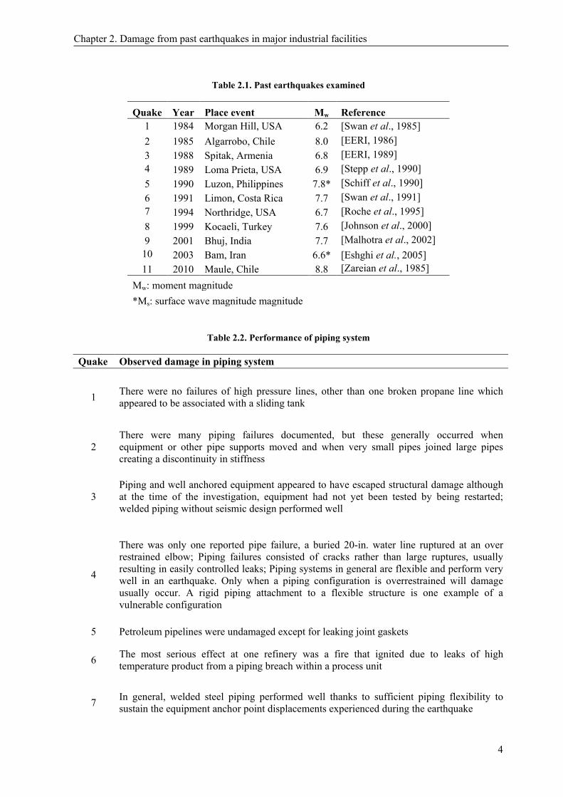
Table 2.1. Past earthquakes examined ..................................................................................................... 4

Table 2.2. Performance of piping system ................................................................................................ 4

Table 2.3. Performance of vessels ........................................................................................................... 5

Table 2.4. Performance of Air Cooler units ............................................................................................. 6

Table 3.1. Piperack masses .................................................................................................................... 17

Table 3.2. Eigenvalues analysis results.................................................................................................. 18

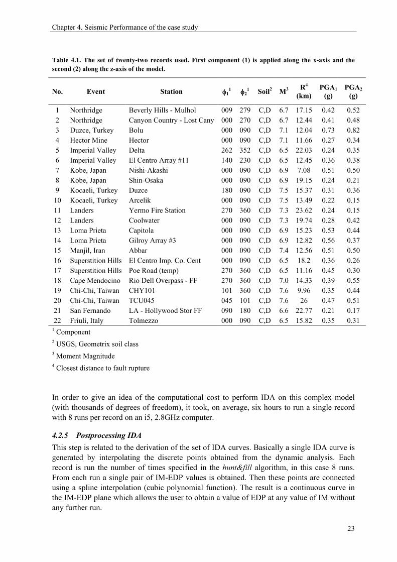
Table 4.1. The set of twenty-two records used. First component (1) is applied along the x-axis and the

second (2) along the z-axis of the model. ..................................................................................... 23

Table 4.2. Median rotational capacities for piping fittings at first leakage............................................ 32

Table 4.3. Summary of first leakage fragility function parameters ....................................................... 32

vii

Chapter 1. Introduction

1 INTRODUCTION

1.1 Motivation The motivation or what where the facts that motivated the election of the Thesis study can be explained by detailing issues around its title: “Seismic risk of industrial plants: assessment of a petrochemical piperack using incremental dynamic analysis”.

First and more general, why industrial plants?

While much of the literature regarding seismic assessment has been developed mainly for residential and office buildings, little information can be found in respect to the type of structures commonly present in industrial facilities with the exception of storage tanks. Industrials facilities such as petrochemical and petroleum plants are by nature a sum of complex structures. The chemical process needed to obtain a specific product or the optimization of an actual one requires the presence of unique pieces of equipment that in turn may need to be supported. As a consequence, either because of geometry or distribution of masses (due to equipment, pipes, platforms, etc.) the resultant structures fall into the category of irregular, or perhaps, special structures, clearly different from the conventional well addressed office buildings. Furthermore, experience from past earthquakes has shown that industrial facilities can be largely damaged although being engineered in compliance with modern codes. The 1988 Armenia and the 1999 Turkey earthquakes are relevant examples [EERI, 1989; Johnson et al., 2000]. Direct and indirect losses together can reach into the order of billions of dollars. These elements (lack of information, special structures, and high risk) are ingredients that motivated the selection of industrial plants. At the same time they are also valid to justify the methodology chosen.

Second, why case study and why a piperack?

Each plant or facility is a unique case since the conditions are always different either due to the owners’ business and strategic interests or because of the site characteristics (earthquake ground motions, type of soil). This uniqueness can be extrapolated to each structure. Nevertheless it is still possible to group and classify the structures into typologies. In this sense, it is believed that piperacks constitute a representative component. Not only because of the kilometres present in a facility, connecting different units and transporting process fluids, but also because they may support key equipment to the operational condition of the plant, such as air coolers equipment.

1

Chapter 1. Introduction

Last, why IDA?

At present, incremental dynamic analysis (IDA) represents the state of the art in analysis methods for seismic assessment. It has been recognized and adopted by several guidelines (e.g. FEMA P-58) and by the research community in numerous studies. One of the advantages of applying IDA is that allows the evaluation of specific objectives (damage states) in agreement with the performance criteria established by the owner. This can be applied either at structural elements (e.g. lateral resisting frames) or nonstructural components (e.g. piping system).

1.2 Objectives The study is limited to the seismic assessment of a typical petrochemical structure. The case study corresponds to a real case, the Main Piperack of a refinery in the Caribbean. The evaluation is focused on capturing the dynamic behaviour of the structure through the application of IDA. Taking advantage of its application, numerical fragility functions will be generated to evaluate the vulnerability of its main nonstructural component, the piping system attached to the air coolers units. The procedure will help to demonstrate the applicability of IDA for industrial structures. It is worth to mention that the procedure can be extended to any damage state of interest in order to evaluate the performance of any component.

1.3 Outline of the Thesis The Thesis consists of four chapters, outlined as follows:

Chapter 2 presents a review of past earthquakes, revising of the typical damage in specific industrial components in order to identify probable failure modes and define associated damage states.

Chapter 3 describes the case study selected to perform the corresponding seismic assessment. Particular details concerning the generation of the numerical model are given here.

Chapter 4 is the key chapter of the Thesis as it presents the results of the assessment through the IDA analysis.

Chapter 5 summarizes the work done in this Thesis and gives suggestions for improvement of the research.

2

Chapter 2. Damage from past earthquakes in major industrial facilities

2 DAMAGE FROM PAST EARTHQUAKES IN MAJOR

INDUSTRIAL FACILITIES

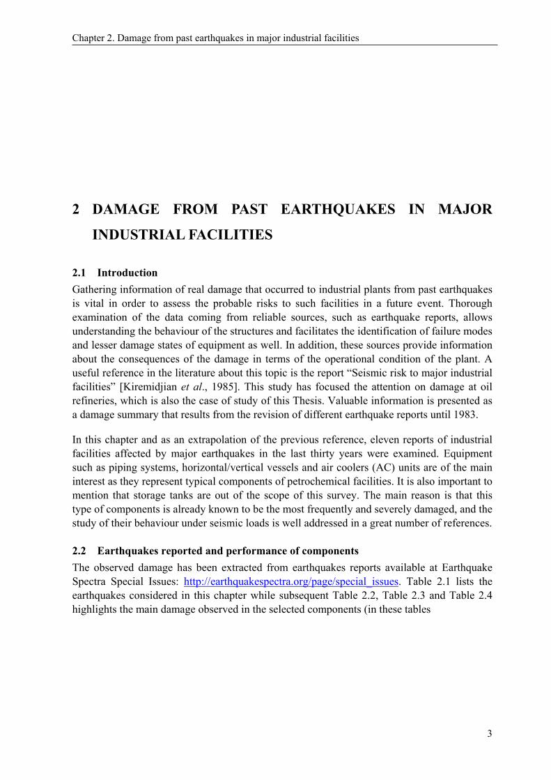
2.1 Introduction Gathering information of real damage that occurred to industrial plants from past earthquakes is vital in order to assess the probable risks to such facilities in a future event. Thorough examination of the data coming from reliable sources, such as earthquake reports, allows understanding the behaviour of the structures and facilitates the identification of failure modes and lesser damage states of equipment as well. In addition, these sources provide information about the consequences of the damage in terms of the operational condition of the plant. A useful reference in the literature about this topic is the report “Seismic risk to major industrial facilities” [Kiremidjian et al., 1985]. This study has focused the attention on damage at oil refineries, which is also the case of study of this Thesis. Valuable information is presented as a damage summary that results from the revision of different earthquake reports until 1983.

In this chapter and as an extrapolation of the previous reference, eleven reports of industrial facilities affected by major earthquakes in the last thirty years were examined. Equipment such as piping systems, horizontal/vertical vessels and air coolers (AC) units are of the main interest as they represent typical components of petrochemical facilities. It is also important to mention that storage tanks are out of the scope of this survey. The main reason is that this type of components is already known to be the most frequently and severely damaged, and the study of their behaviour under seismic loads is well addressed in a great number of references.

2.2 Earthquakes reported and performance of components The observed damage has been extracted from earthquakes reports available at Earthquake Spectra Special Issues: http://earthquakespectra.org/page/special_issues. Table 2.1 lists the earthquakes considered in this chapter while subsequent Table 2.2, Table 2.3 and Table 2.4 highlights the main damage observed in the selected components (in these tables

3

http://earthquakespectra.org/page/special_issues


Table 2.1. Past earthquakes examined

Quake Year Place event Mw Reference 1 1984 Morgan Hill, USA 6.2 [Swan et al., 1985] 2 1985 Algarrobo, Chile 8.0 [EERI, 1986] 3 1988 Spitak, Armenia 6.8 [EERI, 1989] 4 1989 Loma Prieta, USA 6.9 [Stepp et al., 1990] 5 1990 Luzon, Philippines 7.8* [Schiff et al., 1990] 6 1991 Limon, Costa Rica 7.7 [Swan et al., 1991] 7 1994 Northridge, USA 6.7 [Roche et al., 1995] 8 1999 Kocaeli, Turkey 7.6 [Johnson et al., 2000] 9 2001 Bhuj, India 7.7 [Malhotra et al., 2002]

10 2003 Bam, Iran 6.6* [Eshghi et al., 2005] 11 2010 Maule, Chile 8.8 [Zareian et al., 1985]

Mw: moment magnitude *Ms: surface wave magnitude magnitude

Table 2.2. Performance of piping system

Quake Observed damage in piping system

1 There were no failures of high pressure lines, other than one broken propane line which appeared to be associated with a sliding tank

2 There were many piping failures documented, but these generally occurred when equipment or other pipe supports moved and when very small pipes joined large pipes creating a discontinuity in stiffness

3 Piping and well anchored equipment appeared to have escaped structural damage although at the time of the investigation, equipment had not yet been tested by being restarted; welded piping without seismic design performed well

4

There was only one reported pipe failure, a buried 20-in. water line ruptured at an over restrained elbow; Piping failures consisted of cracks rather than large ruptures, usually resulting in easily controlled leaks; Piping systems in general are flexible and perform very well in an earthquake. Only when a piping configuration is overrestrained will damage usually occur. A rigid piping attachment to a flexible structure is one example of a vulnerable configuration

5 Petroleum pipelines were undamaged except for leaking joint gaskets

6 The most serious effect at one refinery was a fire that ignited due to leaks of high temperature product from a piping breach within a process unit

7 In general, welded steel piping performed well thanks to sufficient piping flexibility to sustain the equipment anchor point displacements experienced during the earthquake

4


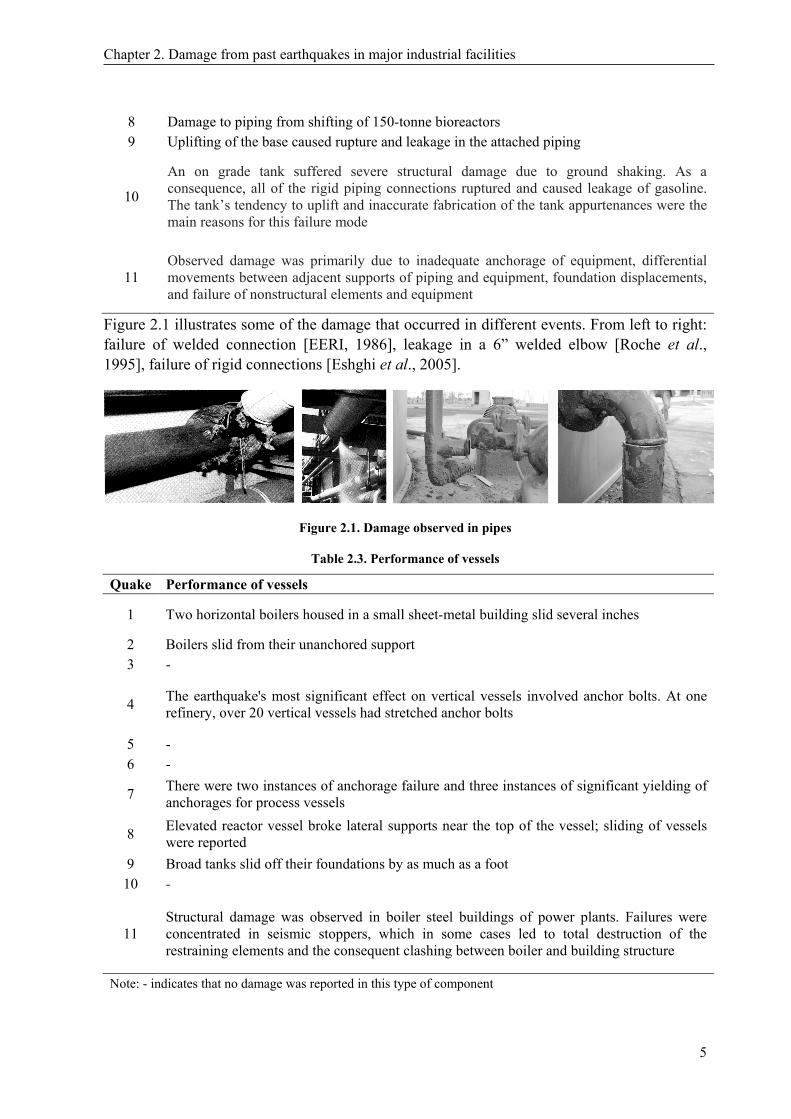
8 Damage to piping from shifting of 150-tonne bioreactors 9 Uplifting of the base caused rupture and leakage in the attached piping

10

An on grade tank suffered severe structural damage due to ground shaking. As a consequence, all of the rigid piping connections ruptured and caused leakage of gasoline. The tank’s tendency to uplift and inaccurate fabrication of the tank appurtenances were the main reasons for this failure mode

11 Observed damage was primarily due to inadequate anchorage of equipment, differential movements between adjacent supports of piping and equipment, foundation displacements, and failure of nonstructural elements and equipment

Figure 2.1 illustrates some of the damage that occurred in different events. From left to right: failure of welded connection [EERI, 1986], leakage in a 6” welded elbow [Roche et al., 1995], failure of rigid connections [Eshghi et al., 2005].

Figure 2.1. Damage observed in pipes

Table 2.3. Performance of vessels

Quake Performance of vessels

1 Two horizontal boilers housed in a small sheet-metal building slid several inches

2 Boilers slid from their unanchored support 3 -

4 The earthquake's most significant effect on vertical vessels involved anchor bolts. At one refinery, over 20 vertical vessels had stretched anchor bolts

5 - 6 -

7 There were two instances of anchorage failure and three instances of significant yielding of anchorages for process vessels

8 Elevated reactor vessel broke lateral supports near the top of the vessel; sliding of vessels were reported

9 Broad tanks slid off their foundations by as much as a foot 10 -

11 Structural damage was observed in boiler steel buildings of power plants. Failures were concentrated in seismic stoppers, which in some cases led to total destruction of the restraining elements and the consequent clashing between boiler and building structure

Note: - indicates that no damage was reported in this type of component

5


Figure 2.2. Shear failure of anchor bolt [Roche et al., 1995] (left and middle);

Sliding of horizontal vessels [Johnson et al., 2000] (right)

Table 2.4. Performance of Air Cooler units

Quake Performance of AC untis (fin fans) 1 - 2 - 3 -

4

(I) The flanges of the supports connecting the fan structure to the battered legs buckled. The braces, which were constructed of light T sections, also buckled, as well as being torn at the supports. The structure lost its capacity to resist seismic forces during this earthquake;(II) All precast beams with fan supports close to their midspan failed in bearing at their seat on the columns. Apparently, the precast beams did not have sufficient bearing capacity

5 - 6 - 7 - 8 - 9 -

10 - 11 -

Note: - indicates that no damage was reported in this type of component

Figure 2.3. Damage to AC support structure [Stepp et al., 1990]

6


2.3 Damage summary Although the performance of a specific plant, structure or component, is case dependent since the number of factors influencing the response is considerable, the repetition of some failure modes makes possible the following summary:

Piping system: The main cause of piping failure is the failure of the connection due to differential movements between anchor points. These might be caused due to:

• Excessive displacements of the structures

• Inadequate anchorage of equipment (e.g., one end is attached to an unanchored equipment that slides or suffers displacements)

• Settlement of the foundation

Vessels: The failure of vessels is rarer than failure of piping. Failure modes have been attributed to:

• Unanchored equipment

• Yielding of anchor bolts

• Failure in shear of anchor bolts with consequent move up of vessel

Air coolers units: Air coolers have failed due to:

• Under sizing of structural support

• Buckling of vertical bracing

• Poor detailing of connections

7

Chapter 3. Description of the case study

3 DESCRIPTION OF THE CASE STUDY

The case study building corresponds to the Main Piperack of the Alkylation Unit of a refinery in the Caribbean. A plan view of the Alkylation unit and the location of the Piperack within it, can be observed in Figure 3.1 and Figure 3.2.

Figure 3.1. Key plan Alkylation Unit

Figure 3.2. Main Piperack south view

8


This structure consists of twenty two transverse steel frames spaced 6.0m each other and connected by longitudinal beams and braces. At frame number twelve, there is an expansion joint that splits the Main Piperack in two smaller and independent piperacks called West and East respectively. For matters of simplicity, in this study the analysis was focused on the West Piperack, hereinafter referred to as the Piperack.

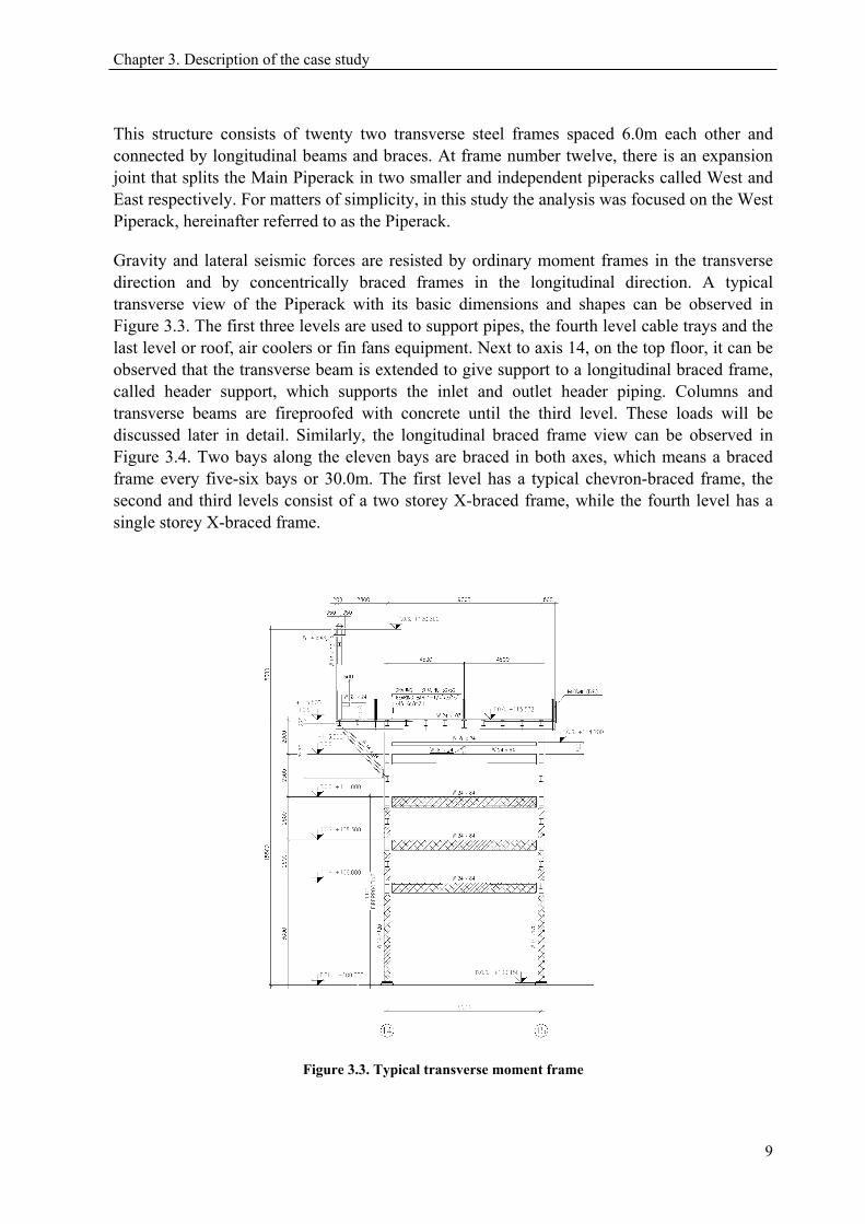
Gravity and lateral seismic forces are resisted by ordinary moment frames in the transverse direction and by concentrically braced frames in the longitudinal direction. A typical transverse view of the Piperack with its basic dimensions and shapes can be observed in Figure 3.3. The first three levels are used to support pipes, the fourth level cable trays and the last level or roof, air coolers or fin fans equipment. Next to axis 14, on the top floor, it can be observed that the transverse beam is extended to give support to a longitudinal braced frame, called header support, which supports the inlet and outlet header piping. Columns and transverse beams are fireproofed with concrete until the third level. These loads will be discussed later in detail. Similarly, the longitudinal braced frame view can be observed in Figure 3.4. Two bays along the eleven bays are braced in both axes, which means a braced frame every five-six bays or 30.0m. The first level has a typical chevron-braced frame, the second and third levels consist of a two storey X-braced frame, while the fourth level has a single storey X-braced frame.

Figure 3.3. Typical transverse moment frame

9


Figure 3.4. Longitudinal braced frame

The roof or top level, where the air coolers are supported, has a steel platform with a floor grating system supported on secondary beams with a complete horizontal bracing system, constituting a rigid diaphragm to avoid relative displacements between transverse frames. Figure 3.5 displays a view in plant of this level.

Figure 3.5. Roof plan view

The steel structure has been designed according to AISC 360-05 specifications (LRFD design method) and UBC-97 seismic code. Columns, beams and braces of the lateral resisting systems are all US W-shapes, ASTM A-36 steel.

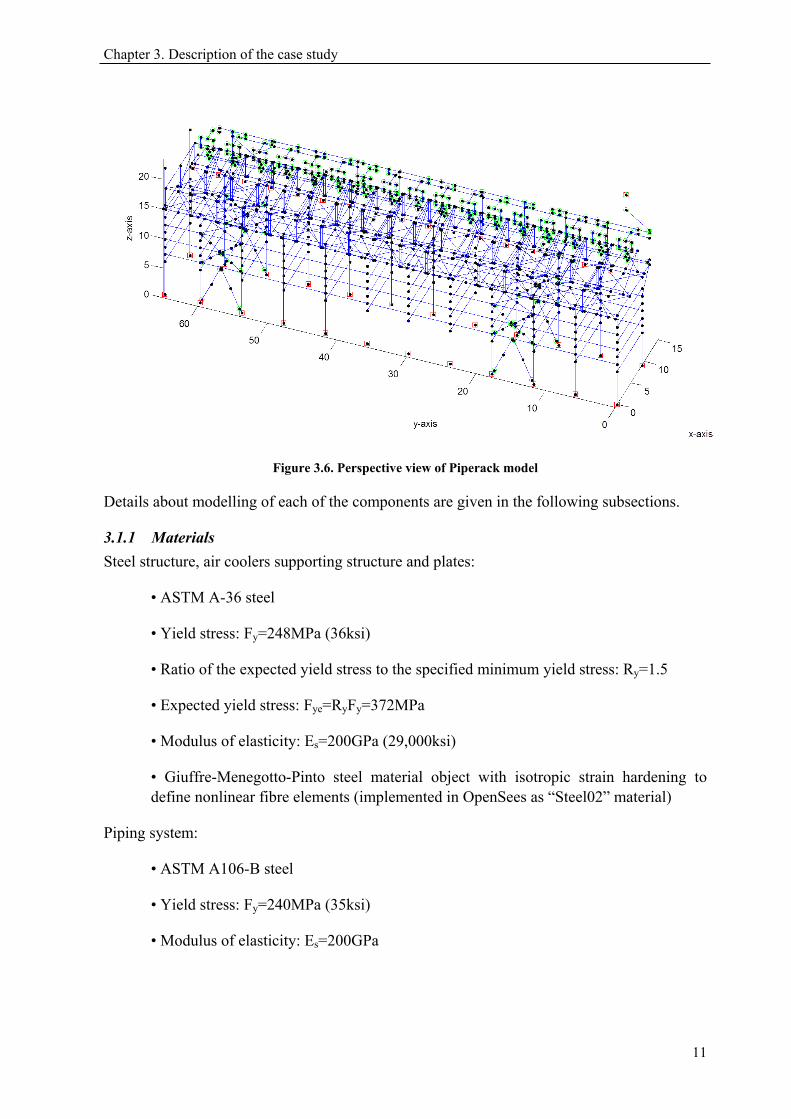
3.1 Description of the analytical model A numerical 3D model was built in the OpenSees structural analysis software platform [McKenna, 1997] in order to simulate the seismic performance. Figure 3.6 shows a perspective view of the model.

10


Figure 3.6. Perspective view of Piperack model

Details about modelling of each of the components are given in the following subsections.

3.1.1 Materials Steel structure, air coolers supporting structure and plates:

• ASTM A-36 steel

• Yield stress: Fy=248MPa (36ksi)

• Ratio of the expected yield stress to the specified minimum yield stress: Ry=1.5

• Expected yield stress: Fye=RyFy=372MPa

• Modulus of elasticity: Es=200GPa (29,000ksi)

• Giuffre-Menegotto-Pinto steel material object with isotropic strain hardening to define nonlinear fibre elements (implemented in OpenSees as “Steel02” material)

Piping system:

• ASTM A106-B steel

• Yield stress: Fy=240MPa (35ksi)

• Modulus of elasticity: Es=200GPa

11


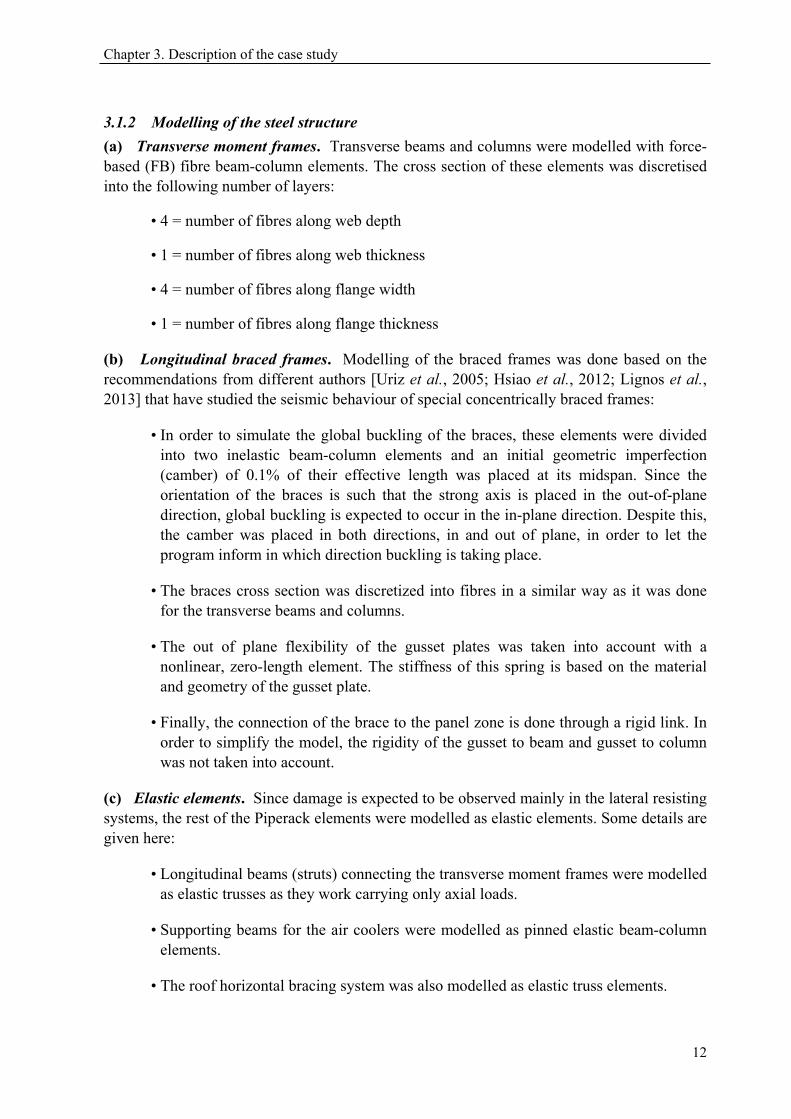
3.1.2 Modelling of the steel structure (a) Transverse moment frames. Transverse beams and columns were modelled with force-based (FB) fibre beam-column elements. The cross section of these elements was discretised into the following number of layers:

• 4 = number of fibres along web depth

• 1 = number of fibres along web thickness

• 4 = number of fibres along flange width

• 1 = number of fibres along flange thickness

(b) Longitudinal braced frames. Modelling of the braced frames was done based on the recommendations from different authors [Uriz et al., 2005; Hsiao et al., 2012; Lignos et al., 2013] that have studied the seismic behaviour of special concentrically braced frames:

• In order to simulate the global buckling of the braces, these elements were divided into two inelastic beam-column elements and an initial geometric imperfection (camber) of 0.1% of their effective length was placed at its midspan. Since the orientation of the braces is such that the strong axis is placed in the out-of-plane direction, global buckling is expected to occur in the in-plane direction. Despite this, the camber was placed in both directions, in and out of plane, in order to let the program inform in which direction buckling is taking place.

• The braces cross section was discretized into fibres in a similar way as it was done for the transverse beams and columns.

• The out of plane flexibility of the gusset plates was taken into account with a nonlinear, zero-length element. The stiffness of this spring is based on the material and geometry of the gusset plate.

• Finally, the connection of the brace to the panel zone is done through a rigid link. In order to simplify the model, the rigidity of the gusset to beam and gusset to column was not taken into account.

(c) Elastic elements. Since damage is expected to be observed mainly in the lateral resisting systems, the rest of the Piperack elements were modelled as elastic elements. Some details are given here:

• Longitudinal beams (struts) connecting the transverse moment frames were modelled as elastic trusses as they work carrying only axial loads.

• Supporting beams for the air coolers were modelled as pinned elastic beam-column elements.

• The roof horizontal bracing system was also modelled as elastic truss elements.

12


Figure 3.7. Modelling of braces

3.1.3 Modelling of the air coolers equipment (a) Description of the equipment operating system. Process air-cooled heat exchangers are designed to condense and cool fluids with high pressure (< 400 bar) in petrochemical and gas plants. Heat exchange surface is made of round finned tubes, fed by inlet and outlet header boxes. Finned tube bundles are installed flat on a structure, they are blown by fans and drivers that are electrically driven. [GEA Heat Exchangers website, http://www.btt-nantes.com/opencms/opencms/btt/en/index.html, 2015].

Figure 3.8. Air coolers operating system

(b) Description of the analytical model. Air coolers equipment has been modelled on top of the Piperack as a one story elastic frame structure, braced in both directions. The geometry and dimensions of the air cooler equipment shown in Figure 3.9 have been obtained from the

13


engineering drawings of the manufacturer [GEA, 2008]. A total of seventeen units of air coolers equipment are supported by the Piperack.

Figure 3.9. Air coolers model

The frame beams representing the rigid box, where the fans, finned tubes and motors are allocated, were modelled as beam-columns elements with high stiffness. The equipment rests on six supporting legs, three displayed in the transverse direction of the piperack and two in the longitudinal direction. They are W6x15 shape columns and were modelled as truss elements. The height of these columns is set equal to the height of the center of mass of the equipment. The columns are directly anchored to longitudinal supporting beams. The lateral braces were modelled as truss elements as usual. All the nodes from the “roof” (or box) were slaved to a master node located at the center of the mass, in order to assure the same translational displacements. The mass of the air cooler was placed in this master node. Gravity loads were applied in correspondence with each column top node and in accordance to their tributary area.

3.1.4 Modelling of the piping system Because of its importance to the plant operating conditions, the piping system under study corresponds to the pipes that connect different pieces of equipment (vessels and exchangers), outside the Piperack, to the air coolers. The remaining piping system that travels along the Piperack in its first three levels is considered only as weight. Figure 3.10 shows a 3D view of the pipe lines considered in the present work.

Details concerning important aspects in the modelling of this particular piping system are given below.

(a) Model for pipes and fittings. Elastic beam elements with hollow sections were used to model straight pipes. Pipe diameters cover a range from 4” to 20”. Pipe wall thickness is specified by its schedule. In this project, all pipes have schedule standard, commonly designated as Sch. Std., which means Sch. 40 for all pipes except for the 20” pipe, which corresponds Sch. 20. The value of the thickness in inches (or mm) can be obtained from ANSI B36.10M tables (e.g. for a 4” Sch. Std., wall thickness is equal to 0.237” or 6.42mm). Pipes material is ASTM A106-B steel. With respect to the fittings or connections, such as welded elbows and tee connections, in order to facilitate the estimation of the rotations at these joints, especially for the tee fittings, the model illustrated in Figure 3.11 was adopted (beam stiffness coefficients figure taken from [Chopra, 1995]).

14


Figure 3.10. 3D view of inlet and outlet header piping

Figure 3.11. Modelling of fittings

15


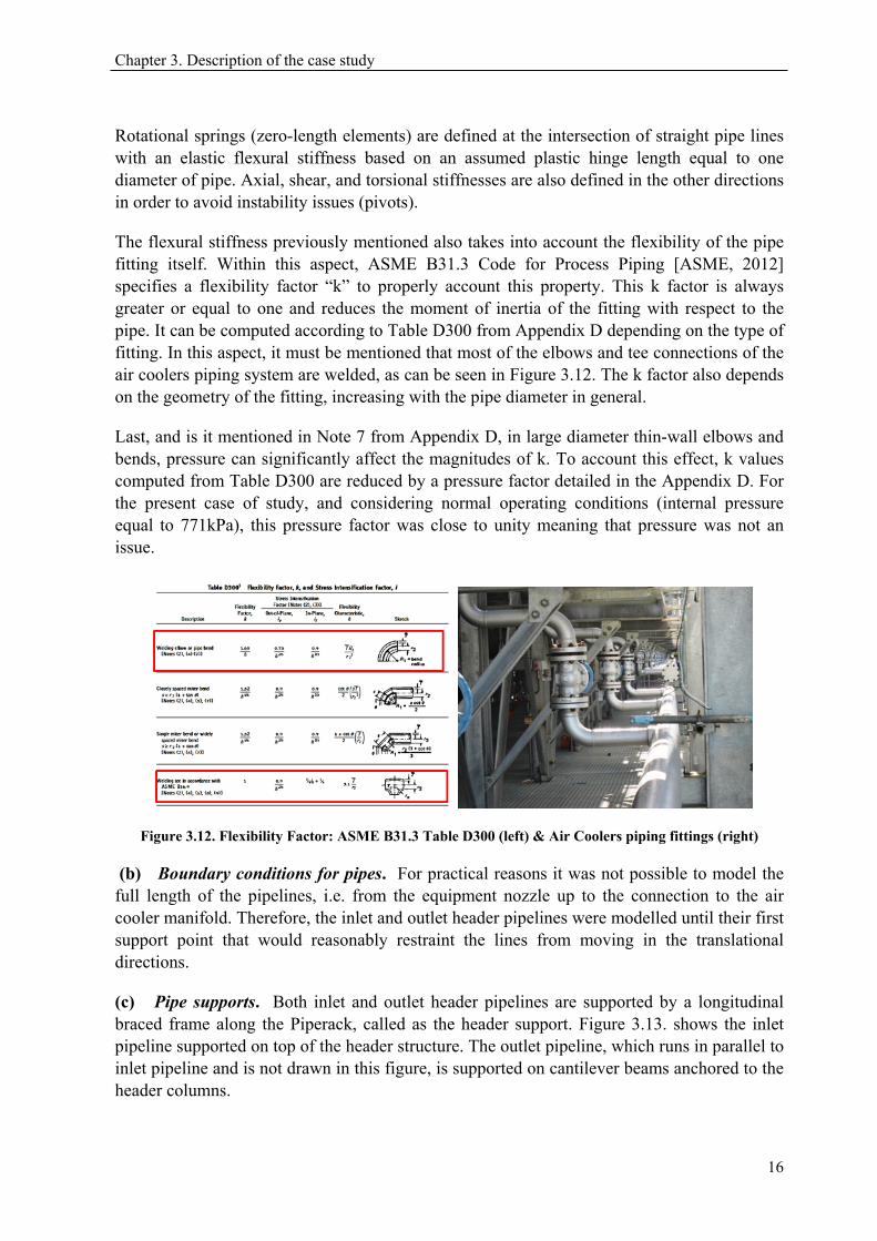
Rotational springs (zero-length elements) are defined at the intersection of straight pipe lines with an elastic flexural stiffness based on an assumed plastic hinge length equal to one diameter of pipe. Axial, shear, and torsional stiffnesses are also defined in the other directions in order to avoid instability issues (pivots).

The flexural stiffness previously mentioned also takes into account the flexibility of the pipe fitting itself. Within this aspect, ASME B31.3 Code for Process Piping [ASME, 2012] specifies a flexibility factor “k” to properly account this property. This k factor is always greater or equal to one and reduces the moment of inertia of the fitting with respect to the pipe. It can be computed according to Table D300 from Appendix D depending on the type of fitting. In this aspect, it must be mentioned that most of the elbows and tee connections of the air coolers piping system are welded, as can be seen in Figure 3.12. The k factor also depends on the geometry of the fitting, increasing with the pipe diameter in general.

Last, and is it mentioned in Note 7 from Appendix D, in large diameter thin-wall elbows and bends, pressure can significantly affect the magnitudes of k. To account this effect, k values computed from Table D300 are reduced by a pressure factor detailed in the Appendix D. For the present case of study, and considering normal operating conditions (internal pressure equal to 771kPa), this pressure factor was close to unity meaning that pressure was not an issue.

Figure 3.12. Flexibility Factor: ASME B31.3 Table D300 (left) & Air Coolers piping fittings (right)

(b) Boundary conditions for pipes. For practical reasons it was not possible to model the full length of the pipelines, i.e. from the equipment nozzle up to the connection to the air cooler manifold. Therefore, the inlet and outlet header pipelines were modelled until their first support point that would reasonably restraint the lines from moving in the translational directions.

(c) Pipe supports. Both inlet and outlet header pipelines are supported by a longitudinal braced frame along the Piperack, called as the header support. Figure 3.13. shows the inlet pipeline supported on top of the header structure. The outlet pipeline, which runs in parallel to inlet pipeline and is not drawn in this figure, is supported on cantilever beams anchored to the header columns.

16


Figure 3.13. Header support structure

Regarding piping supports where longitudinal displacements are allowed, friction between the steel pipe and the steel support has been modelled through zero-length elements with an elasto-plastic material (“ElasticPP” material) to resemble the Coulomb friction model. In this case, and following a similar design criterion, the yield strength was computed taking into account the static friction factor (µ = 0.3).

3.1.5 Modelling of masses Masses supported by the Piperack structure were lumped at frame nodes only with translational components. Table 3.1 summarises the values computed at each level.

Air cooler mass was lumped at the equipment center of mass in correspondence with the master node as previously mentioned. Each equipment weight is equal to 247.3kN. Regarding the inlet/outlet header piping although they are mainly distributed masses along the length of the pipes, to simplify the analysis, they were lumped at its model nodes. It must be mentioned that the piping operating fluid is steam (gas), hence the weight is all attributed to pipe selfweight, fittings and valves.

Table 3.1. Piperack masses

Level Elevation Steel Str. FireProof. Piping Grating AC Total Mass Ratio [ - ] [m] [ton] [ton] [ton] [ton] [ton] [ton] [-] 1 5.55 47.2 118.5 49.5 0.0 0.0 215.2 0.16 2 8.05 38.9 100.7 71.6 0.0 0.0 211.1 0.16 3 10.55 38.9 67.9 31.8 0.0 0.0 138.6 0.10 4 13.05 28.2 0.0 128.8 0.0 0.0 157.0 0.12 5 15.05 110.2 0.0 27.2 38.1 428.6 604.1 0.46

Total Total 263.3 287.1 309.0 38.1 428.6 1326.1 1.00

3.2 Modal analysis: Eigenvalues The results of the modal analysis are presented below. The first fifteen periods with their corresponding effective masses are listed in Table 3.2. The dominant modes are T1=0.881sec and T7=0.468sec corresponding to the transverse (moment frames) and longitudinal (braced frames) direction. The rest of the periods are associated with local modes of excitation of the piping system. The modal shapes of the structure in both directions are illustrated in Figure 3.14 and Figure 3.15.

17


Table 3.2. Eigenvalues analysis results

Number Period Effective Mass [ - ] [sec] x y T1 0.881 0.902 0.006 T2 0.848 0.000 0.021 T3 0.812 0.003 0.004 T4 0.787 0.006 0.017 T5 0.734 0.003 0.023 T6 0.704 0.001 0.000 T7 0.468 0.003 0.856 T8 0.466 0.002 0.036 T9 0.353 0.001 0.000

T10 0.340 0.006 0.001 T11 0.334 0.055 0.000 T12 0.305 0.002 0.000 T13 0.284 0.000 0.000 T14 0.269 0.000 0.000 T15 0.261 0.000 0.001

Figure 3.14. Modal shape in transverse direction T1=0.881sec

0 5 1015

010

2030

4050

60

0

5

10

15

20

EigenVector 1

18


Figure 3.15. Modal shape in longitudinal direction T7=0.468sec

05

1015

010

2030

4050

60

0

5

10

15

20

EigenVector 7

19

Chapter 4. Seismic Performance of the case study

4 ASSESSMENT OF THE CASE STUDY USING

INCREMENTAL DYNAMIC ANALYSIS

4.1 Introduction In this chapter, the seismic performance of the Main Piperack (descripted in the previous chapter) is assessed applying incremental dynamic analysis (IDA). Our goal is to evaluate the behaviour of the steel structure under a suite of ground motions records, focusing the attention on the response of the piping system attached to the Air Coolers equipment.

First, a brief description of the method is presented, summarizing the main steps to be followed for the analysis of this practical case. Then certain details concerning the application of the method are given. The results of the nonlinear analysis are presented as a set of IDA curves and its statistical summary into three fractiles. In order to validate them and gain understanding, static pushover analysis (SPO) was carried out and its results were then plotted in the same IDA fractiles chart for comparison and discussion. Last, and in order to put on evidence the seismic vulnerability, numerical fragility functions were built for the piping system taking advantage of the IDA.

4.2 Incremental Dynamic Analysis (IDA) The following paragraphs intend to be a summary of the aforementioned method and have been written considering the main concepts from its original publications [Vamvatsikos and Cornell, 2002; Vamvatsikos and Cornell, 2004]. In addition, the analysis and subsequent postprocessing routines have been carried out applying the related software tools from: http://users.ntua.gr/divamva/software.html

4.2.1 Description of the method It can be said that the original concept of IDA, scaling an acceleration time-history, was re-developed and put it into a solid and unified method in response to the Performance-Based Earthquake Engineering (PBEE). This framework, which appeared in the late nineties, was intrinsically requiring a strong analysis method that could be able to estimate demands and responses at any level of seismic intensity, in order to satisfy different and specific performance objectives.

IDA is a parametric analysis method and involves performing multiple nonlinear dynamic analyses of a structural model under a suite of ground motion records, each scaled to several

20

http://users.ntua.gr/divamva/software.html


levels of seismic intensity [Vamvatsikos and Cornell, 2002]. The scaling levels are appropriately selected to force the structure go through the entire range of behaviour, from elastic to inelastic and finally to global dynamic instability, where the structure essentially experiences collapse. Appropriate postprocessing can present the results in terms of IDA curves, one for each ground motion record, of the seismic intensity, typically represented by a scalar Intensity Measure (IM), versus the structural response, as measured by an Engineering Demand Parameter (EDP). It is important to mention that although IDA can be argued to fail in the ability to use different records at each level of intensity, thus potentially resulting to large scaling factors [Luco and Bazzurro, 2007], it still remains a viable alternative when wanting to assess the vulnerability of a structure with as little connection to a specific site as possible.

IDA process can be summarized into the following steps [Vamvatsikos and Cornell, 2004]:

• Definition of the IM and the EDP(s)

• Selection of the records

• Dynamic analysis of the structural model

• Postprocessing of results

• Definition of limit states and estimation of its capacities

4.2.2 Definition of the main variables: IM and EDP(s) IM: the 5% damped spectral acceleration of the structure’s first-mode period (transverse direction of the structure), was selected to characterize the intensity of the ground motion, and was used for scaling of the records.

• IM = Sax (T1, 5%),

EDP: the selection of the EDP depends on the damage state of interest and it is obviously case dependent. Therefore two EDPs were defined, one to monitor the performance of the steel structure itself, and a second one to estimate the damage in the piping system. Therefore:

• Steel structure EDP = peak interstorey drift ratio, θmax

• Piping system EDPi = peak rotation at fitting "i", θmax, fitt i

With respect to the first one, it can be mentioned that this is a common EDP for steel buildings since it is well related to the damage that occurs in structural typologies, such as moment frames and braced frames.

The selection of the second EDP has to do with the fact that experience has shown that most failures of piping systems of this type, occur within the joint connections. Furthermore the rotations can be perfectly tracked thanks to the definition of rotational springs at each piping joint facilitating the postprocessing.

21


4.2.3 Suite of ground motions: ATC-63 When performing IDA on a 3D structural model, two components of ground motions are needed. Also, the nonlinear analysis requires equally scaling both components of each record. For this study the selected suite corresponds to the “Set One: Basic far-field ground motion set selected without considering Epsilon (reduced)” from [Haselton et al., 2007]. It consists of 22 records with two horizontal components extracted from the original set of 39 records. Details are given in Table 4.1. The same set was used in the Applied Technology Council Project 63, which was focused on developing a procedure to validate seismic provisions for structural design.

The set consists of selected strong ground motions that may cause the structural collapse of modern buildings. Some of the selection criteria are the following:

• Magnitude > 6.5

• Distance from source to site > 10 km

• Peak ground acceleration > 0.2g and peak ground velocity > 15 cm/sec

• Soil shear wave velocity, in upper 30m of soil, greater than 180 m/sec (NEHRP soil types: A–D; note that all selected records happened to be on C/D sites)

4.2.4 Performing IDA After defining the main elements for performing IDA (IM, EDPs, ground motions), the next step is to run the nonlinear dynamic analysis. A key aspect when running multiple records is to minimize the number of runs for each record without compromising the accuracy and resolution of the final IDA curve. In other words, it is vital the use of an appropriate algorithm that will make this step a more efficient one.

The present work has applied the hunt&fill tracing algorithm [Vamvatsikos and Cornell, 2001] which aims with the above mentioned issues at reducing the computational efforts. Further details on how it works can be found in this last reference. The following parameters have been specified to define the hunt&fill algorithm:

• Initial step = 0.1g

• Step increment = 0.2g

• Allowed number of runs per record = 8

An additional condition has been specified to trace the IDA curve: the algorithm will not increase the intensity level if a maximum interstory drift of 10% limit is exceeded (in the transverse direction, x). This requirement has to do with the fact that there is no practical interest to go beyond such high EDP level.

22


Table 4.1. The set of twenty-two records used. First component (1) is applied along the x-axis and the second (2) along the z-axis of the model.

No. Event Station φ11 φ2

1 Soil2 M3 R4 (km)

PGA1 (g)

PGA2 (g)

1 Northridge Beverly Hills - Mulhol 009 279 C,D 6.7 17.15 0.42 0.52 2 Northridge Canyon Country - Lost Cany 000 270 C,D 6.7 12.44 0.41 0.48 3 Duzce, Turkey Bolu 000 090 C,D 7.1 12.04 0.73 0.82 4 Hector Mine Hector 000 090 C,D 7.1 11.66 0.27 0.34 5 Imperial Valley Delta 262 352 C,D 6.5 22.03 0.24 0.35 6 Imperial Valley El Centro Array #11 140 230 C,D 6.5 12.45 0.36 0.38 7 Kobe, Japan Nishi-Akashi 000 090 C,D 6.9 7.08 0.51 0.50 8 Kobe, Japan Shin-Osaka 000 090 C,D 6.9 19.15 0.24 0.21 9 Kocaeli, Turkey Duzce 180 090 C,D 7.5 15.37 0.31 0.36

10 Kocaeli, Turkey Arcelik 000 090 C,D 7.5 13.49 0.22 0.15 11 Landers Yermo Fire Station 270 360 C,D 7.3 23.62 0.24 0.15 12 Landers Coolwater 000 090 C,D 7.3 19.74 0.28 0.42 13 Loma Prieta Capitola 000 090 C,D 6.9 15.23 0.53 0.44 14 Loma Prieta Gilroy Array #3 000 090 C,D 6.9 12.82 0.56 0.37 15 Manjil, Iran Abbar 000 090 C,D 7.4 12.56 0.51 0.50 16 Superstition Hills El Centro Imp. Co. Cent 000 090 C,D 6.5 18.2 0.36 0.26 17 Superstition Hills Poe Road (temp) 270 360 C,D 6.5 11.16 0.45 0.30 18 Cape Mendocino Rio Dell Overpass - FF 270 360 C,D 7.0 14.33 0.39 0.55 19 Chi-Chi, Taiwan CHY101 101 360 C,D 7.6 9.96 0.35 0.44 20 Chi-Chi, Taiwan TCU045 045 101 C,D 7.6 26 0.47 0.51 21 San Fernando LA - Hollywood Stor FF 090 180 C,D 6.6 22.77 0.21 0.17 22 Friuli, Italy Tolmezzo 000 090 C,D 6.5 15.82 0.35 0.31

1 Component 2 USGS, Geometrix soil class

3 Moment Magnitude 4 Closest distance to fault rupture

In order to give an idea of the computational cost to perform IDA on this complex model (with thousands of degrees of freedom), it took, on average, six hours to run a single record with 8 runs per record on an i5, 2.8GHz computer.

4.2.5 Postprocessing IDA This step is related to the derivation of the set of IDA curves. Basically a single IDA curve is generated by interpolating the discrete points obtained from the dynamic analysis. Each record is run the number of times specified in the hunt&fill algorithm, in this case 8 runs. From each run a single pair of IM-EDP values is obtained. Then these points are connected using a spline interpolation (cubic polynomial function). The result is a continuous curve in the IM-EDP plane which allows the user to obtain a value of EDP at any value of IM without any further run.

23


The complete set of IDA curves generated for the piperack is presented in two plots: Figure 4.1. Twenty-two IDA curves for the maximum interstory drift in the transverse direction (Moment Frames) corresponds to the transverse direction (Moment Frames), while Figure 4.3 corresponds to the longitudinal direction (Braced Frames). The black dots on the IDA curves correspond to the discrete points obtained from the analysis and mentioned in the previous paragraph.

Both plots are useful to confirm some of the general properties of IDA curves mentioned in [Vamvatsikos and Cornell, 2002]:

• Record to record variability: the same structure behaves differently from record to record despite the fact that the selected records have similar characteristics.

• Type of behaviours: IDA curves corresponding to pure softening case, pure hardening case and weaving behaviour can be observed.

Also by comparing both plots, it is evident that the braced frames have a higher elastic stiffness and a shorter elastic range than the moment frames, as expected.

What is next presented is the summary of the IDA curves in Figure 4.2 and Figure 4.4. The complete set of twenty-two IDA curves can be summarized into their corresponding 16, 50 and 84% fractiles curves. It can be said that the 50% fractile will show a central value, while the 16 and 84% fractiles will provide a measure of dispersion of the data. These curves were obtained by computing cross sectional fractiles of the EDP at each level of intensity (horizontal stripes).

The main conclusion from this analysis is that the piperack structure collapses or reaches the 10% drift stop limit at very high IM levels. The same commentary applies for lower and common drift limits, for example the ones that define the immediate occupancy (IO) (lowest IM limit state). For instance, if we consider the 50% fractiles for the braced frames, this IO is violated for Sax (T1, 5%)=0.52g or (θmax=0.5% according to FEMA 356)

4.2.6 SPO vs IDA To better understand the behaviour of the piperack and the interpretation of their IDA curves as well, nonlinear static pushovers (SPO) were carried out. The type of integrator used for this analysis was displacement control and the lateral loads (reference loads) along the height of the structure were defined according to the ASCE07-10 distribution. The node control is at the top of the structure and belongs to the frame with largest tributary loads. Figure 4.5 illustrates this step. A peak in the load pattern can be observed at the roof level due to the high masses of the AC equipment.

24


Figure 4.1. Twenty-two IDA curves for the maximum interstory drift in the transverse direction (Moment Frames)

Figure 4.2. The corresponding 16, 50 and 84% fractile IDA curves of Figure 4.1

0 0.05 0.1 0.15 0.20

0.5

1

1.5

2

2.5

3

3.5

4

"fi

rst-m

ode"

spe

ctra

l acc

eler

atio

n S a(T

1,5%

) (g)

maximum interstory drift ratio, θ max

0 0.05 0.1 0.15 0.20

0.5

1

1.5

2

2.5

3

3.5

4

"firs

t-mod

e" s

pect

ral a

ccel

erat

ion

S a(T1,5

%) (

g)


16% fractile50% fractile84% fractile

25


Figure 4.3. Twenty-two IDA curves for the maximum interstory drift in the longitudinal direction (Braced Frames)

Figure 4.4. The corresponding 16, 50 and 84% fractile IDA curves of Figure 4.3

0 0.05 0.1 0.15 0.20

0.5

1

1.5

2

2.5

3

3.5

4

"fi

rst-m

ode"

spe

ctra

l acc

eler

atio

n S a(T

1,5%

) (g)


0 0.05 0.1 0.15 0.20

0.5

1

1.5

2

2.5

3

3.5

4

"firs

t-mod

e" s

pect

ral a

ccel

erat

ion

S a(T1,5

%) (

g)


16% fractile50% fractile84% fractile

26


The results from the analysis are pictured in Figure 4.6. In order to visualize the effects of P-Delta, two type of analysis were considered: one accounting for these geometric nonlinear effects and the other one neglecting them. This can be issued in OpenSees by appropriate setting of the geometric transformation command.

By observing the curves corresponding to the moment frames, results clearly show that the P-Delta effects reduce the post-yield stiffness, from positive to practically zero in the X-direction. Large inelastic deformation is observed and target displacements can be easily reached (e.g., in this direction the structure was pushed up to an 8% drift ratio).

On the contrary, brittle behaviour corresponding to the braced frames is observed. The pushover curve starts with an elastic stiffness higher than the one corresponding to the moment frame, but soon after it reaches its peak in strength, it abruptly drops indicating the first buckling of the braces. Then it continues to gain strength at a lower slope than the initial one, until a second drop is observed, indicative of a second buckled brace. A third example of this behaviour is also seen.

Figure 4.5. SPO load pattern for both directions

27


Figure 4.6. SPO in both directions with and without P-Delta effects

Figure 4.7. SPO vs IDA - Moment Frame (left), zoom (right)

Figure 4.8. SPO vs IDA - Braced Frame (left), zoom (right)

0 0.05 0.1 0.15 0.2 0.25 0.3 0.35 0.4 0.45 0.50

2000

4000

6000

8000

10000

12000

roof displacement, δ roof (m)

tota

l bas

e sh

ear,

V base

(kN

)

Moment Frame with P-∆ (X)Moment Frame w/o P-∆ (X)Braced Frame with P-∆ (Y)Braced Frame w/o P-∆ (Y)

0 0.02 0.04 0.06 0.08 0.1 0.12 0.14 0.16 0.18 0.20

0.5

1

1.5

2

2.5

3

3.5

4


"firs

t-mod

e" s

pect

ral a

ccel

erat

ion

S a(T1,5

%) (

g)

0 0.005 0.01 0.015 0.02 0.025 0.03 0.035 0.040

0.2

0.4

0.6

0.8

1

1.2

1.4

1.6

1.8

2


"firs

t-mod

e" s

pect

ral a

ccel

erat

ion

S a(T1,5

%) (

g)

0 0.02 0.04 0.06 0.08 0.1 0.12 0.14 0.16 0.18 0.20

0.5

1

1.5

2

2.5

3

3.5

4


"firs

t-mod

e" s

pect

ral a

ccel

erat

ion

S a(T1,5

%) (

g)

0 0.005 0.01 0.015 0.02 0.025 0.03 0.035 0.040

0.2

0.4

0.6

0.8

1

1.2

1.4

1.6

1.8

2


"firs

t-mod

e" s

pect

ral a

ccel

erat

ion

S a(T1,5

%) (

g)

28


It is interesting to put the SPO curves into the IDA chart or IM-EDP plane. This step requires expressing the base shear computed in the SPO process into spectral acceleration terms. Although it may not be completely accurate, but acceptable for the qualitative purposes, this was done dividing the base shear by the total weight of the structure in order to have it expressed in terms of gravity acceleration (g). The results shown in Figure 4.7 and Figure 4.8 demonstrate the expected good agreement between the SPO curve and the 50% fractiles IDA for the elastic branch.

4.3 Seismic vulnerability of the AC piping system The seismic vulnerability of a structural or nonstructural component can be graphically represented through the generation of numerical fragility functions (or curves). Therefore their importance in a seismic assessment procedure. A component fragility function for a given damage state provides the probability that the component will be in that damage state (DS) or worse after experiencing any given value of an IM. This definition implies first defining an EDP that is appropriate for monitoring the performance with respect to the DS. This was already specified in section 4.2.2, where peak rotations at each fitting were stated to be the EDP for the piping system. Then it is necessary to define an EDPcap threshold value (or capacity) that marks the onset of the DS itself. Details regarding the DS and the EDPcap are given in following sections. The above mentioned can be expressed by the following:

Fragility = 𝑃𝐷𝑆(𝑥) = 𝑃( 𝑉𝑖𝑜𝑙𝑎𝑡𝑖𝑛𝑔 𝐷𝑆 | 𝐼𝑀 = 𝑥) (4.1)

Fragility = 𝑃𝐷𝑆(𝑥) = 𝑃�𝐸𝐷𝑃(𝑥) ≥ 𝐸𝐷𝑃𝑐𝑎𝑝 � 𝐼𝑀 = 𝑥) (4.2)

A lognormal cumulative distribution function (CDF) is often assumed in this type of applications to define a fragility function. A CDF is characterized by two parameters, the median of the fragility function θ (the IM level with 50% probability of equalling or exceeding the DS) and β, the standard deviation of ln IM (sometimes referred to as the dispersion of IM):

𝐹𝑟𝑎𝑔𝑖𝑙𝑖𝑡𝑦 = 𝑃𝐷𝑆(𝑥) = Φ�ln (𝑥/𝜃)

𝛽� (4.3)

4.3.1 Definition of Damage State (DS) A damage state describes the level of damage experienced by a component or system to a certain IM. In this study the following single DS was considered:

• DSi = first leakage of piping fitting (corresponding to diameter “i”)

Experimental test done in pipe joints suggests that first leakage either occurs simultaneously or before yielding/failure of the pipe. Once a pipe has leaked, it must be replaced automatically, lowering the functionality of AC equipment. Therefore it is believed that the selected DS is representative of the seismic performance of the piping system and by extrapolation, the AC equipment.

29


4.3.2 Rotational capacity of fittings at first leakage (EDPcap) To completely define the previous DS is vital to set appropriate values of EDP at which the DS occurs in a particular fitting. Unfortunately, in comparison to structural components and systems, there is relatively limited information on the seismic performance of piping fittings. Although numerous piping codes and guidelines can be found on the literature, they basically present limiting values expressed in terms of stress-strain which are not useful for this approach.

With the above in mind, the capacities for each pipe diameter were computed taking into account the experimental research work carried at the University of Buffalo [Tian et al., 2014]. In this study experimental fragility data was developed for sprinkler piping joints of different materials and connection types up to 6” diameter. Furthermore, this study provides the following expression to extrapolate the results for larger diameters not tested:

𝜃𝑙𝑒𝑎𝑘 =2�̅�𝐷0

(4.4)

where θ leak is the median rotational capacity at first leakage; D0 (in.) is the outside pipe diameter; 𝑠� is the average axial slip (analogous to strain in bending assuming plane sections remain plane) and is a constant value of 0.019in. for threaded pipe joints. It is important to highlight that rotational capacities for welded joints adopted/computed from this reference should give considerably conservative results since a few experimental tests done for welded joints indicated a much stiffer behaviour than the threaded ones.

4.3.3 Piping fittings monitored for fragility functions Although recorders of rotations were placed in every single fitting of the entire piping system (i.e. the complete piping system can be monitored), the fragility functions were computed based on the rotations of three pipe diameters: 4”, 6” and 8”. This decision was taken based on the fact that using Equation (4.4) to extrapolate for larger diameters (e.g. 16” or 20”) could not be accurate. Figure 4.9 highlights the “reduced” piping system (nevertheless, 83% of the modelled piping system) and its corresponding sections.

Figure 4.9. Piping system monitored for fragility functions

30


4.3.4 Estimation of fragility functions using fitting IDA curves IDA curves for each fitting of the piping system were obtained in the same way IDA curves were built for the piperack structure (moment and braced frames). As an example, Figure 4.10 illustrates twenty-two IDA curves obtained for six pipe fittings. Given the large number of fittings monitored (510 fittings), it is not feasible to plot them all.

Figure 4.10. Examples of IDA curves obtained for piping fittings: 4”(top); 6”(middle); 8”(bottom)

With these fittings IDA curves it is possible to generate fragility functions by taking stripes of EDP given a certain IM level. Those values of EDP, each one corresponding to one record, are used to compute the probability of reaching or exceeding the EDPcap defined by the CDF of the piping component (see values in Table 4.2). As each record in the stripe is an independent, equiprobable sample, the probability is obtained simply by counting the fraction

0 0.5 1 1.5 2 2.5 3 3.5

x 10-3

0

0.5

1

1.5

2

2.5

3

3.5

4

"firs

t-mod

e" s

pect

ral a

ccel

erat

ion

S a(T1,5

%) (

g)

maximum rotation at fitting, θ max fitt

0 0.5 1 1.5 2 2.5 3 3.5

x 10-3

0

0.5

1

1.5

2

2.5

3

3.5

4

"firs

t-mod

e" s

pect

ral a

ccel

erat

ion

S a(T1,5

%) (

g)maximum rotation at fitting, θ

max fitt

0 0.5 1 1.5 2 2.5 3 3.5

x 10-3

0

0.5

1

1.5

2

2.5

3

3.5

4

"firs

t-mod

e" s

pect

ral a

ccel

erat

ion

S a(T1,5

%) (

g)


0 0.5 1 1.5 2 2.5 3 3.5

x 10-3

0

0.5

1

1.5

2

2.5

3

3.5

4

"firs

t-mod

e" s

pect

ral a

ccel

erat

ion

S a(T1,5

%) (

g)


0 0.5 1 1.5 2 2.5 3 3.5

x 10-3

0

0.5

1

1.5

2

2.5

3

3.5

4

"firs

t-mod

e" s

pect

ral a

ccel

erat

ion

S a(T1,5

%) (

g)

maximum rotation at fitting 4, θ max fitt 4

0 0.5 1 1.5 2 2.5 3 3.5

x 10-3

0

0.5

1

1.5

2

2.5

3

3.5

4

"firs

t-mod

e" s

pect

ral a

ccel

erat

ion

S a(T1,5

%) (

g)

maximum rotation at fitting 2, θ max fitt 2

31


of records that cause the exceedance of the EDP capacity value. This step is repeated for the whole range of IM of interest. By connecting these points, pairs of probability of exceedance (PoE) and IM values, a numerical “empirical” CDF is obtained for the DS considered. The term empirical refers to the fact that the fragility uses only the data coming from analysis, without any fitting of a parametric distribution.

Table 4.2. Median rotational capacities for piping fittings at first leakage

Pipe diameter Experiment Eq. (4.4) Interp.

[in] θleak βθ leak θleak βθ leak

4" 0.010 0.216 - - 6" 0.006 0.204 - - 8" - - 0.004 0.192

Interp.: linear interpolation between two tested diameters

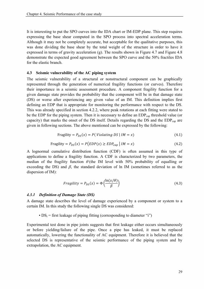
Naturally, this stepped empirical CDF can be fitted to obtain a smoothed curve. Under the assumption that it follows a lognormal distribution, two common methods were used to obtain their parameters, i.e. the median IM (in terms of spectral acceleration) and its dispersion.The first method is the moment matching lognormal fit: basically will use PoE=50% to get the median and PoE=16, 84% to define the dispersion (the distance between the 16% and 84% values is twice the std-log of data, or the dispersion, for a lognormal distribution).The second method applied is the maximum likelihood lognormal fit, which keeps the same concept doing the fit with an improved algorithm of the previous by selecting the parameters that maximizes the likelihood function (http://en.wikipedia.org/wiki/Maximum_likelihood). The fragility functions corresponding to the empirical CDF and the two fits, for each DS (diameter dependent), are graphically presented in Figure 4.11, Figure 4.12 and Figure 4.13. In addition, the final parameters obtained from the fitting process can be found in Table 4.3.

Finally, a simplistic and rapid way to combine the three different fragility functions into a resultant one to be used for assessing the the first “absolute” leakage (regardless the pipe diameter), is to take the maximum PoE from the three curves for each level of IM. Although the results could be judged to be unconservative since the appropriate (and laborious) way would imply to consider conditional probabilities for each level of IM and record, they might be useful to provide first cut estimate to be later improved.

Table 4.3. Summary of first leakage fragility function parameters

Pipe diameter Moment-fit MLE-fit [in] Ŝa leak (g) βŜa leak Ŝa leak (g) βŜa leak

4" 2.868 0.686 2.153 0.734 6" 3.573 0.362 3.122 0.353 8" 2.507 0.442 2.342 0.452

Combination 2.507 0.675 2.011 0.693 Ŝa leak (g): median “first mode” spectral acceleration at first leakage

βŜa leak: logarithmic standard deviation (dispersion)

32

http://en.wikipedia.org/wiki/Maximum_likelihood


Figure 4.11. Fragility functions for 4" pipe fitting

Figure 4.12. Fragility function 6" pipe fitting

Figure 4.13. Fragility function 8" pipe fitting

0 0.5 1 1.5 2 2.5 3 3.5 40

0.1

0.2

0.3

0.4

0.5

0.6

0.7

0.8

0.9

1

"first-mode" spectral acceleration Sa(T1,5%) (g)

Pro

babi

lity

of e

xcee

danc

e, P

DS

Actual data (Empirical CDF)Lognormal moments-fitLognormal MLE-fit

0 0.5 1 1.5 2 2.5 3 3.5 40

0.1

0.2

0.3

0.4

0.5

0.6

0.7

0.8

0.9

1


Pro

babi

lity

of e

xcee

danc

e, P

DS


0 0.5 1 1.5 2 2.5 3 3.5 40

0.1

0.2

0.3

0.4

0.5

0.6

0.7

0.8

0.9

1


Pro

babi

lity

of e

xcee

danc

e, P

DS


33


Figure 4.14. Fragility function regardless pipe diameter

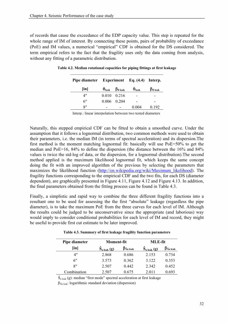
4.3.5 Visualizing the piping DS on piperack IDA curves An interesting way to graphically link the performance of the steel structure and the piping system, is to plot a point on each of the piperack IDA curves, this is one point for each record, indicating the occurrence of the first fitting leakage regardless of its diameter (first “absolute” leakage). See Figure 4.15 below.

Again this can be done by looking individually, for each diameter and record, at the corresponding spectral acceleration at which first leakage occurs. Then by comparing the values for the three diameters, the minimum will be the one of interest. Finally with this minimum spectral acceleration the corresponding interstorey drift is obtained to define the pair of values needed to plot the point on its corresponding IDA curve.

Figure 4.15. Leakage point on piperack IDA curves: Moment frame (left) ; Braced frame (right)

0 0.5 1 1.5 2 2.5 3 3.5 40

0.1

0.2

0.3

0.4

0.5

0.6

0.7

0.8

0.9

1


Pro

babi

lity

of e

xcee

danc

e, P

DS


0 0.05 0.1 0.15 0.20

0.5

1

1.5

2

2.5

3

3.5

4

"firs

t-mod

e" s

pect

ral a

ccel

erat

ion

S a(T1,5

%) (

g)


0 0.05 0.1 0.15 0.20

0.5

1

1.5

2

2.5

3

3.5

4

"firs

t-mod

e" s

pect

ral a

ccel

erat

ion

S a(T1,5

%) (

g)


34

Chapter 5. Conclusions

5 CONCLUSIONS

5.1 Summary This study has carried out a specific seismic assessment of a piperack structure that is representative of those found in many industrial plants. The case study corresponded to a modern facility in a highly seismic area as it is the Caribbean. This structure supports nonstructural components considered vital for the operability of the plant. Therefore, it is of paramount importance to evaluate its seismic performance.

An initial and necessary revision of past earthquakes was done in Chapter 2. As it was expected this examination showed important evidence of damage, which in turn contributed to define the damage state to monitor.

In order to assess the performance of the piperack a numerical model was built as described in Chapter 3. This step demanded an important effort in time due to the complex geometry of the structure plus the large number of nonstructural elements to model. Simplified models would be needed here to accelerate this step and to allow evaluating larger number of components

Once the numerical modelled was completed, a rigorous methodology was needed to assess the response of the piperack. IDA was selected given its capability to capture the full range of structural behaviour under seismic loads. The possibility of using the software tools developed by the original authors was of great help and made the analysis and postprocessing very efficient.

Chapter 4 contains the final output. A full set of IDA curves obtained for the steel structure illustrates the peculiar behaviour that this structure follows in the inelastic range. In summary, the collapse appears to happen only at very high ground motion intensities. IDA curves were then compared to SPO curves to validate the agreement in the elastic range. Finally the convolution of IDA curves obtained for the fittings of the AC piping system with the fragility functions of these components, permitted the generation of new fragility functions in terms of spectral acceleration. These curves demonstrated that the damage state of first leakage will have a low probability of occurrence for this piperack. This result may be a consequence of the small relative displacements between structure and AC and to the fact that pipe guidelines used for the design are well known to be quite conservative.

35

Chapter 5. Conclusions

5.2 Future work The following are suggestions for future (or continuation of this) work come from limitations by time-frame of the Thesis:

• Evaluation of other typologies present in industrial plants (e.g. reactors or vessels supporting structure), ranked according to their potential risks and importance to the operability of the plant.

• Generation of simplified yet sufficiently accurate models that allow running more analyses and evaluating different components.

• Consideration of a secondary IM, i.e. using a geometric mean of Sa at different periods to account for spectral shape and/or the two orthogonal directions.

• Evaluation of additional limit states of engineering and stakeholder significance, e.g., percentage of pipes leaking, movement of heavy equipment (air coolers), etc.

• Computation of mean annual frequencies of violating the limit states (convolution with probabilistic seismic hazard analysis (PSHA) for the specific site)

It is worth mentioning that this work would have benefitted from further experimental data for piping fittings of diameters comparable to those considered in this study.

36

References

REFERENCES

American Lifelines Alliance, 2002, Seismic Design and Retrofit of Piping Systems.

ASME B31.3, 2012, Code for Process Piping, American Society of Mechanical Engineers, New York, NY (Revision of ASME B31.3-2010).

Bursi, O. S., Reza, M. S., Abbiati, G., Paolacci, F. [2015] “Performance-based earthquake evaluation of a full-scale petrochemical piping system,” Journal of Loss Prevention in the Process Industries, Vol. 33, pp. 10-22.

Chopra, A. K. [1995] “Dynamics of Structures Theory and Applications to Earthquake Engineering”, Prentice Hall, Upper Saddle River, NJ

EERI [1986], “The Chile Earthquake of March 3, 1985—Industrial Facilities”, Earthquake Spectra, Vol. 2, No. 2, pp. 373-409.

EERI [1989], “Performance of industrial facilities”, Earthquake Spectra, Vol. 5, No. S1, pp. 101-113.

Haselton, C.B. and G.G. Deierlein [2007] “Assessing Seismic Collapse Safety of Modern Reinforced Concrete Frame Buildings”, Blume Earthquake Engineering Research Center

Hsiao, P. C., Lehman, D. E., Roeder, C. W. [2012], “A Model to Simulate Special Concentrically Braced Frames Beyond Fracture”, Earthquake Engineering & Structural Dynamics, EESD, doi: 10.1002/eqe.2202.

Kiremidjian, A. S., Ortiz, K., Nielsen, R., and Safavi, B. [1985]. “Seismic Risk to Major Industrial Facilities”, Report to the National Science Foundation, Grant No. CEE-8116997 and CEE-8400479.

Johnson, G. S., Aschheim, M., Sezen, H. [2000], “Industrial Facilities”, Earthquake Spectra, Vol. 16, No. S1, pp. 311-350.

Malhotra, P. K., Rajaram, S.K., Namjoshi, R., Srinivasan, S., Rao, D.S., Gupta, A., Ballantyne, D. [2002], “Industrial Facilities”, Earthquake Spectra, Vol. 18, No. S1, pp. 257-264.

McKenna, F. [1997]. “Object oriented finite element programming frameworks for analysis, algorithms and parallel computing.” Ph.D. thesis, University of California, Berkeley, CA.

Lignos, D. G., Karamanci, E. [2013], “Predictive equations for modeling cyclic buckling and fracture of steel braces”, Proceedings of 10th International Conference on Urban Earthquake Engineering, Tokyo, Japan.

37

References

Luco, N., Bazzurro, P. [2007], “Does Amplitude Scaling of Ground Motion Records Result in Biased Nonlinear Structural Drift Responses?”, Earthquake Engineering & Structural Dynamics, EESD, Vol. 36, Issue 13, pp 1813–1835.

Paolacci, F., Reza, M. S., Bursi, O. [2011] “Seismic analysis and component design of refinery piping systems” Proceedings of 3rd International Conference on Computational Methods in Structural Dynamics and Earthquake Engineering, Corfu, Greece.

Roche, T., Merz, K., Burger, P., Doran, G., McCabe, E., Nitta, S., Ostrom, D., Rothemich, V., Watts, D., White, W. [1995], “Industry”, Earthquake Spectra, Vol. 11, No. S2, pp. 245-285.

Soroushian S., Maragakis M., Zaghi A.E., Echevarria A., Tian Y., Filiatrault A. [2013], “Numerical seismic fragility of fire sprinkler piping systems with threaded joints”, Proceedings of 10th International Conference on Urban Earthquake Engineering, Tokyo, Japan.

Schiff, A.J. [1991], “Petroleum and gas facilities”, Earthquake Spectra, Vol. 7, No. S2, pp. 49-58.

Stepp, J. C., Swan, S., Wesselink, L., Haupt, R.W., Larder, R.R., Bachman, R.E., Malik, L., Eli, M., Porush, A. [1991], “Industrial facilities”, Earthquake Spectra, Vol. 6, No. S1, pp. 189-238.

Swan, S.W., Miller, D.D., Yanev, P.I. [1985], “The Morgan Hill Earthquake of April 24, 1984—Effects on Industrial Facilities, Buildings, and Other Facilities”, Earthquake Spectra, Vol. 1, No. 3, pp. 457-568.

Swan, S.W., O. Hamburger, R. [1991], “Industrial facilities”, Earthquake Spectra, Vol. 7, No. S2, pp. 49-58.

Task Committee on Seismic Evaluation and Design of Petrochemical Facilities of ASCE [2011], Guidelines for Seismic Evaluation and Design of Petrochemical Facilities: Second Edition, ASCE

Tian, Y., Filiatrault, A., Mosqueda, G., [2014]. “Experimental seismic fragility of pressurized fire suppression sprinkler piping joints”, Earthquake Spectra, Vol. 30, No. 4, pp. 1733-1748.

Uriz, P., Filippou, F.C., Mahin, S.A. [2008] “Model for Cyclic Inelastic Buckling of Steel Braces”,. Journal of Structural Engineering, 134(4):619–628.

Uriz, P., Filippou, F.C., Mahin, S.A. [2008] “Model for Cyclic Inelastic Buckling of Steel Braces”,. Journal of Structural Engineering, 134(4):619–628.

Vamvatsikos D., Cornell C.A. ,[2001] “Tracing and post-processing of IDA curves: Theory and software implementation”. Report No. RMS-44, RMS Program, Stanford University, Stanford.

Vamvatsikos D., Cornell C.A. [2002], “Incremental dynamic analysis”, Earthquake Engineering and Structural Dynamics, 31, 491-514.

Vamvatsikos D., Cornell C.A. [2004], “Applied incremental dynamic analysis”, Earthquake Spectra, 20, 523-553.

Vamvatsikos D., Sigalas I. [2005], “Seismic performance evaluation of a horizontally curved highway bridge using incremental dynamic analysis in 3D”, Proceedings of the 4th European Workshop on the seismic behaviour of irregular and complex structures, Thessaloniki, Greece.

Zareian, F., Sampere, C., Sandoval, V., McCormick, D.L., Moehle, J., Leon, R. [2012], “Reconnaissance of the Chilean Wine Industry Affected by the 2010 Chile Offshore Maule Earthquake”, Earthquake Spectra, Vol. 28, No. S1, pp. S503-S512.

38

Documents

SEISMIC RISK OF INDUSTRIAL PLANTS: ASSESSMENT …users.ntua.gr/divamva/docs/StuMS/Danesi_MSThesis2015.pdf · The dissertation entitled “Seismic Risk of Industrial Plants: Assessment