Embed Size (px)
Citation preview

B A H R A M H O U C H M A N D Z A D E H
S E L E C T E D L E C T U R E SI N P H Y S I C S .

Université Grenoble-AlpesPhysics Department
No rights reserved. Every part of this manuscript may be repro-duced, modified or transmitted without the author’s acknowl-egdment.The author will greatly appreciate the readers feedbacks/ criticisms/error corrections.
web : http://wwwliphy.ujfgrenoble.fr/pagesperso/bahram/M1_Nano/M1_nano.htmlB : bahram.houchmandzadeh à univ-grenoble-alpes.frFirst version : August 28th, 2016Present version : November 20, 2018

Contents
I Mathematics 7
1 Analysis. 91.1 The concept of function. 11
1.2 Exercises: functions. 18
1.3 Weighting functions. 21
1.4 Exercises: Weighting functions. 26
1.5 The concept of differentiation. 27
1.6 Exercises: differentiation. 35
1.7 The concept of integration. 37
1.8 Exercises: integrations. 45
1.9 Application of infinitesimal calculus. 48
1.10 Approximating functions : Taylor expansion. 50
1.11 Exercises : Taylor expansion. 52
1.12 Appendix. 53
2 Differential equations. 572.1 A tale of treasure Island. 58
2.2 Linear first order equation. 59
2.3 Exercises: First Order equations. 67
2.4 Linear second order differential equation. 70
2.5 Solving a system of ODEs. 73
2.6 Numerical solution of ODE. 74
2.7 Exercises. 74
CONTENTS 4
3 Complex numbers. 753.1 Numbers and algebra. 753.2 Complex numbers. 763.3 Usual Operations. 763.4 Application to forced harmonic oscillator. 773.5 Exercises. 78
4 The Fourier Series. 814.1 Definition. 824.2 The idea of basis in the function space. 824.3 Examples of Fourier series. 854.4 Sine and Cosine series. 854.5 Complex Fourier series. 864.6 The vibrating string. 874.7 Some other Orthogonal bases. 884.8 The Fourier Transform. 88
5 Linear Algebra. 915.1 Why linear algebra is such a fundamental topic. 925.2 Linear systems. 925.3 Vectors. 935.4 Linear Application. 965.5 Solving a linear system. 965.6 Numerical methods. 975.7 Eigenbasis and matrix diagonalization. 975.8 Tensors. 97
II Physics 99
6 Mechanics. 1016.1 Fundamental concepts. 1026.2 The fundamental law of mechanics. 1056.3 Exercises: Movement. 1156.4 Kinetic energy, work, power. 118

5 CONTENTS
6.5 Potential and total energy. 119
6.6 Exercises : Energy 122
6.7 Equilibrium. 125
6.8 Exercises: Equilibrium. 129
6.9 The Lagrangian formulation. 131
6.10 Exercises: Lagrangian. 137
6.11 Advanced topics: Relativity. 138
6.12 Application: the principle of an atomic force microscope. 139
7 Electrical circuits. 1417.1 Introduction and definitions. 143
7.2 The Ohm’s law. 149
7.3 Energy and power. 156
7.4 The AC revisited. 157
7.5 Generalizing circuits. 164
7.6 Exercises. 166
8 Thermodynamics. 1678.1 The concept of energy. 169
8.2 Temperature. 170
8.3 Energy transfer. 171
8.4 Extensive and intensive parameters. 172
8.5 Heat capacity. 173
8.6 Work. 174
8.7 Equilibrium, reversible and irreversible changes. 176
8.8 Entropy. 177
8.9 Application to Perfect gases. 178
8.10 The thermal machine: Carnot cycle. 185
8.11 The thermodynamic potential F and the minimum principle. 189
8.12 Change of variables and generalized potentials. 193
8.13 The Maxwell relations. 198
8.14 Statistical Physics. 201

CONTENTS 6
9 Optics. 2079.1 Introduction. 2089.2 Ray optics. 2089.3 Image Formation. 2099.4 Exercises. 2179.5 Beyond geometrical optics : wave optics and interference. 2199.6 Basics of spectroscopy. 219
10 Quantum Mechanics. 22110.1 A philosophical tale about elephants. 22210.2 The vibrating string. 222

Part I
Mathematics


Chapter 1
Analysis.
Contents
1.1 The concept of function. 11
1.1.1 Function as an idealization of measurements. 11
1.1.2 Graphical representation of functions. 12
1.1.3 Algebraic functions. 12
1.1.4 The inverse function. 13
1.1.5 Exponential and logarithm. 14
1.1.6 Trigonometric functions. 16
1.1.7 Multivalued functions. 17
1.1.8 Change of variable. 17
1.2 Exercises: functions. 18
1.3 Weighting functions. 21
1.3.1 Weighting powers. 22
1.3.2 Weighting the inverse function. 23
1.3.3 Weighting specific functions close to zero. 24
1.3.4 Weighting specific functions close to arbitrary point. 25
1.4 Exercises: Weighting functions. 26
1.5 The concept of differentiation. 27
1.5.1 Definition. 27
1.5.2 Notations and function approximations. 28
1.5.3 Derivative of addition and product. 29
1.5.4 Derivative of combined functions. 30
1.5.5 Derivative of the inverse function. 31
1.5.6 Partial derivative. 32
1.5.7 Derivative of implicit functions. 33
1.5.8 Local extrema of a function. 33
1.5.9 Drawing curves. 34
1.6 Exercises: differentiation. 35

CHAPTER 1. ANALYSIS. 10
1.7 The concept of integration. 37
1.7.1 Integral definition. 37
1.7.2 Properties of the integral. 38
1.7.3 Geometric interpretation of integration. 39
1.7.4 Functions defined by an integral. 39
1.7.5 Fundamental theorem of analysis. 39
1.7.6 Change of variable. 41
1.7.7 Integration by part. 43
1.8 Exercises: integrations. 45
1.9 Application of infinitesimal calculus. 48
1.9.1 49
1.10 Approximating functions : Taylor expansion. 50
1.10.1 Revisiting the differential. 50
1.10.2 Taylor approximation. 50
1.11 Exercises : Taylor expansion. 52
1.12 Appendix. 53
1.12.1 manipulating the symbol∑. 53
1.12.2 The Euler number e. 54

11 1.1. THE CONCEPT OF FUNCTION.
1.1 The concept of function.
1.1.1 Function as an idealization of measurements.
“Mensuro ergo sum”1 wasn’t said by a famous philosopher, even 1 I measure, therefore I exist
though humans have an obsession with measurements. A very earlyexample of measurement was for example the elevation of the sunat noon as the day passed, which gave a very precise tool to Egyp-tians to predict Nile’s flood and allowed the Babylonian to prepareextremely precise calendars.
Nowadays, the act of measurement is so ubiquitous that we tendnot to notice it. We can summarize this act by saying that we havetwo quantities (days and sun’s elevation, acid concentration andPH, height of an object and its speed as it touches the floor, ...)which are measurable and related. For simplicity, let us call themx and y 2. We make a two columns (or two rows) table in which 2 or † and + or whatever is simple
and suits youwe report the joined measurements of these two quantities. As wehave a tendency to organize things, we sort (say in ascending order)one of the columns (say the first one) for later ease of reference. Letus suppose that x is the temperature and y is the viscosity of thewater. If we are a careful experimenter, we may measure values oftemperature (x) in the range of 2 to 100C, by sampling every 1C(table 1.1). If we need more precision, we can redo the measurementsevery 0.01 or 0.001C.
T ν
2 1.6733 1.6194 1.5675 1.5186 1.4727 1.4278 1.38560 0.46665 0.43370 0.40475 0.37780 0.354
Table 1.1: Temperature (°C)and viscosity (MPa.s) of water.
Once we have made this measurement, we can answer the ques-tion “what is the water viscosity at 25C” or “at which temperaturedo we measure viscosity of 1.3847” by consulting this table. If wehad sampled the temperature every 0.1C, we cannot in principle an-swer the question “what is the viscosity of water at T =3.05. Wecan however make a good guess by looking up the value we have atone step above and below this temperature and make an average ofthem.
the concept of function is an idealization of these kind of ta-bles, by supposing that the sampling has been performed for everyreal value of x in a given range [a, b]. For each function, we havea unique table and vice et versa. Of course, as we live in the realworld, our power of sampling is limited and the best computingdevice we have will always have a small but non-zero sampling preci-sion. In the following, we will often denote the sampling value as h,having in mind that for mathematicians, h is as small as we wish.
Figure 1.1: Function f(.) as adevice
Let us suppose that we denote a given table (a function) by thesymbol f(.). Another way of picturing a function is to imagine adevice which does the search in the table f(.) in our place : whenwe ask “what is the value on the right column of f(.) when on theleft column we have the value x ?”, the device look up the wholetable and produces the correct answer. We can then picture a givenfunction as a black box device which when presented with a giveninput, produces a given output.
Notation 1 In the following, afunction with a name such as f willbe denoted by the symbol f(.), orwhen there is no ambiguity, simplyby f . The value this functionproduces for a given input x will bedenoted f(x). Note that f(x) isjust a number, while f(.) is a wholetable.

CHAPTER 1. ANALYSIS. 12
1.1.2 Graphical representation of functions.
As humans, we evolved in an environment where some senses becameimportant to deal with the outside world. The sense we rely heavilyon is the vision and our neural processing unit (brain) is very (very) good at interpreting signals from the eye sensor. On the otherhand, dealing with numbers and tables of numbers were of extremelypoor value to hunt the mammoth and escape from the lion. As wehave the same brain than 100000 years ago, we still rely heavily ongeometrical processing.
Figure 1.2: The curve C = Pnis the graphical representationof the function f(.)
Some 400 years ago, Descartes found a very smart way of repre-senting a function ( i.e. a table of numbers) with a graph (a geomet-rical representation). The recipe is the following: We can represent anumber by its position along a given line. Now take two orthogonalaxes ; a couple of numbers (x, y) is represented in such a way thatits projection on the horizontal axis is x and on the vertical line is y.Now, for a whole table which we call a function f(.), take each rowwith its two numbers (xi, yi) and find the corresponding point Pi onthe plane. Do that for all rows of the table. The collection of pointsPi (which we call a curve) is the graphical representation of thefunction f(.) (fig. 1.2).
Note that a graphical representation is just that: a representation.If bats had came upon the cognitive branch of evolution (instead ofhumans), they would have probably developed a sound representa-tion of functions. When computers will reach the sentient stage, theywill forgo the graphical representation as their processing unit hasevolved to deal with numbers (and poorly with geometry).
1.1.3 Algebraic functions.
Representing functions by tables is heavy. Few decades ago, wewould have in our libraries shelves full of books which containedjust these kind of tables, and when you needed the precise value of afunction for a given value, you would scan a given book.
Some functions however can be represented by a rule which sum-marizes the whole table. Consider a table which is produced in thefollowing way : for each value x on the left column, the right columncontains the number 2x+ 3. If we have 3.1415926 on the left side,we would have 9.2831852 on the right side. The whole table can thusbe summarized by the rule “right column = twice left column plusthree”. We need only 42 character to summarize an infinite table!
The relative number of these kind of functions (compared to allfunctions) is ... zero. They are however very dear to us humans,allowing us to bypass storing infinite shelves of tables. We will seeexactly how in due course.
The simplest such function is called the identity function, whichwe will denote by X(.). The X(.) function produces an output iden-tical to its input: X(x) = x. The function we discussed above can

13 1.1. THE CONCEPT OF FUNCTION.
therefore be written f(.) = 2X(.) + 3 or even simpler,
f = 2X + 3
§ 1.1 What is the meaning of the functions X2 − 4 and 1 +X +X2/2 +
X3/3 ?
Definition 1 Functions of the type3 3 For the meaning and manipula-tion of the symbol
∑, see appendix
1.12.1 on page 53.P =
N∑i=0
aiXi
where ai are numbers are called polynomials. For a given value x,
P (x) =
N∑i=0
aixi
What are the arithmetic operations we can perform exactly onnumbers ? Obviously, addition, subtraction, multiplication and di-vision make it up to the list. So we can combine these operations toproduces more complicated functions than polynomials. For exam-ple, let P1 and P2 be two polynomials, the function
Q = P1/P2
for a given input x produces Q(x) = P1(x)/P2(x).Root extraction is not an exact operation: we don’t have any
finite algorithm to produce exactly the square root of a number4. 4 The question of√
2 has apparentlyled to a homicide in ancient greece.However, we can perform root extraction to any desired precision
by an algorithm which uses only the four basic arithmetic opera-tion, so we will add this operation (and by extension, the n−th rootextraction) to the list of what we know. All these operations arecalled algebraic, and any function which can be summarized by acombination of these operation is called an algebraic function.
§ 1.2 What is the meaning of the function
6
√X2 − 4
1 +X +X2/2 +X3/3
The majority of functions around are not algebraic. We can how-ever very decently approximate them with such functions as we willlearn below.
1.1.4 The inverse function.
Figure 1.3: A function andits inverse, as different way ofconsulting the same table.
Let us come back to the function f(.) as a two column table, wherethe values to one column are referred to by x and in the other col-umn by y. Usually we put the column containing the x’s on the leftand the y’s on the right (fig. 1.3). The function f(.) allows one toanswer the question “ for a given value x, what is the value f(x)?”. The same table however allows to answer an other interestingquestion: “if I have a particular value y on the right, which value xI have on the left” ? Consulting the table by the y column is calledthe inverse function. We are creature of habit, so to answer the sec-ond kind of question, we make a new table where the y column is

CHAPTER 1. ANALYSIS. 14
put on the left and then, the inverse function is symbolically writtenf−1(.) (fig. 1.4).
The graphical representation of the inverse function is obtainedby a mirror symmetry operation, where the mirror is placed on thediagonal line (fig. 1.5).
Figure 1.4: The same table asin (1.3), where the columnshave been exchanged in orderfor the consulting to be fromleft to right.
§ 1.3 Plot the function X2(.) and its inverse.
Let us consider the square function f(.) = X2(.) and its corre-sponding table. This function outputs the square of the number onits input. If we ask “what is f(2)”, by looking up the left columnof the table until finding 2 and then moving to the right column (orperforming the operation 2× 2), we find the answer 4.
Now, we can consult the table on the reverse order, which we callf−1(.). To find the answer f−1(4), we look up the table on the rightcolumn until finding 4, then move to the left column and come upwith the answer 2.
Figure 1.5: if the blue curve Cis the graphical representationof f(.), then the red curve C−1
is the representation of f−1(.).
We could also answer the question by reformulating the question: “which number, when squared, will produce 4 ? To answer thisquestion, we will scan the left column, for each value we look, wecheck if the answer is correct. If the answer is not correct, we moveto the next row until we find the correct answer 2. Both these pro-tocols (looking the right column or checking the left column) willproduce the correct value. Usually, we use the first protocol when wehave a computable rule (a formula ) for the inverse function f−1(.).When we have only a computable rule for the direct function f(.),the second protocol is used.
The inverse of the function X2 is called the square root√X or
X1/2. As we said before, the function X1/2 is not computable (bythe four basic arithmetic operations) and indeed, we find its valueby the second protocol. Of course, we have developed algorithms tospeed up the search and we don’t scan all the numbers one by one.In general, the inverse of the function Xn is the n−th root functionX1/n.
In general, we assume that if we know a function f , we also knowits inverse f−1, even though the practical computation of f−1 can betime consuming. This is why we have included the root extraction inthe basic arithmetic operations. 5 5 the notation f−1 is an unfortunate
one, as usually x−1 denotes the func-tion 1/x. The reader is supposed touse wisely this notation and alwaysmake the difference between the twomeaning represented by the samenotation.
Finally, let us note that the inverse of inverse function is thefunction itself:
(f−1)−1 = f
1.1.5 Exponential and logarithm.
Very early on, the map makers and people looking to the skieslearned that there are very useful functions which are not algebraic.Some of the widely used non-algebraic functions are the power (andits inverse, the logarithm) and the trigonometric functions such assin(.) and cos(.).
Let us introduce the power function fa such that f(x) = ax.For each value of a, we have a different function. Given a value of

15 1.1. THE CONCEPT OF FUNCTION.
a, we can compute for example fa(1) = a, fa(2) = a × a andfa(3) = a× a× a. In order to compute f(1/2), we just take thesquare root of a : fa(1/2) =
√a; by the same token, fa(3/2) =√
a× a× a. Using the same kind of computations, we are able tocompute fa(p/q) for any integers p and q. As any real number canbe approximated to the desired precision by a couple of integers pand q, we assume that we know the value fa(x) for any real x. Notetwo very important property of the power function:
fa(x+ y) = fa(x)fa(y) (1.1)fa(0) = 1 (1.2)
§ 1.4 Demonstrate property (1.1). Begin to demonstrate that for (i) inte-gers ; (ii) for numbers of the form 1/p (using inverse functions), (iii) thengeneralize to arbitrary rationals p/q.
§ 1.5 How would you justify property (1.2) ? Consider numbers of the form1/p for larger and larger p.
Among all fa functions, two are widely used : f10 and fe where eis called the Euler number6 e = 2.71828... For the first function, we 6 We will get to this number later on,
when we will see approximation bymolynomials
have for example f10(2) = 100, f10(−1) = 0.1 and so on. Its valuefor integer arguments is easily computed by appropriately adding 0in front or behind the number 1. The second function is not as easilycomputable. It has a very nice property however which we will seelater. It is so widely used that it has received a proper name: theexponential function.
The inverse of the function fa(.) = a(.) is called the logarithmfunction in base a:
loga(.) = f−1a (.)
The logarithm function was first discovered (or invented, dependingon your philosophical view of mathematics) by Napier around ∼1600 and it has such nice properties that it became a cornerstone ofapplied mathematics for the next 400 years. Usually, the most usedfunction in applied mathematics is log10(.), for which we have forexample log10(100) = 2 and log10(0.1) = −1.
§ 1.6 What is log10(10x) ?
The most used logarithm function in general is loge(.) whichwe will simply note log in these lectures (the notation ln, naturallogarithm, is also used).
Some of the nice properties of the logarithm function are thefollowing:
loga(xy) = loga(x) + loga(y) (1.3)loga(xα) = α loga(x) (1.4)
§ 1.7 Using the concept of inverse function, demonstrate relations (1.3,1.4).
The above properties made the logarithm very popular. Addingtwo numbers is easy ; multiplying them however is more tricky. Soinstead of multiplying two numbers x and y, we will first compute
CHAPTER 1. ANALYSIS. 16
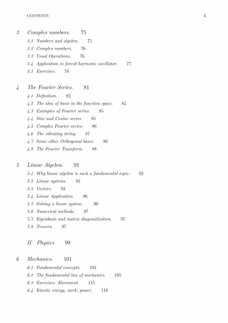
their logarithm log(x) and log(y)(usually by consulting a logarithmtable), add these two numbers z = log(x) + log(y) and then tak-ing the antilogarithm (the inverse function) r = az) using the sametable, and voilà: r = xy. The process can be used to make cumber-some computation such a 6.58922/3 × 1543.41/2. Logarithm tablestherefore became an indispensable equipment of any engineer ormathematician. A mechanical device called the slide rule was eveninvented to speed up the logarithm table consultation and until1960’s wa the standard tool of engineers until electronic calculatorsreplaced them.
0 0.1 0.2 0.3 0.4 0.5 0.6 0.7 0.8 0.91 0.000 0.041 0.079 0.114 0.146 0.176 0.204 0.230 0.255 0.2792 0.301 0.322 0.342 0.362 0.380 0.398 0.415 0.431 0.447 0.4623 0.477 0.491 0.505 0.519 0.531 0.544 0.556 0.568 0.580 0.5914 0.602 0.613 0.623 0.633 0.643 0.653 0.663 0.672 0.681 0.6905 0.699 0.708 0.716 0.724 0.732 0.740 0.748 0.756 0.763 0.7716 0.778 0.785 0.792 0.799 0.806 0.813 0.820 0.826 0.833 0.8397 0.845 0.851 0.857 0.863 0.869 0.875 0.881 0.886 0.892 0.8988 0.903 0.908 0.914 0.919 0.924 0.929 0.934 0.940 0.944 0.9499 0.954 0.959 0.964 0.968 0.973 0.978 0.982 0.987 0.991 0.996
Table 1.2: Table of logarithms,from 1.0 to 9.9. The first digitis read on the raws, the seconddigit on columns. For example,log10(1.3) = 0.114
§ 1.8 using logarithm table.Using Table 1.2, find 2.1× 3.6 ; 12/4.7,
√8.7 ; 5.28 and 100.93. Usually,
the logarithm table are given to at least a precision of two digits.
1.1.6 Trigonometric functions.
Consider a circle of radius R with two perpendicular axes (figure1.6). The angle θ is defined as the normalized arc length betweentwo points along the circle θ = `/R. The normalized projection ofpoint at angle θ with one axis on the two axes are called cos(θ) andsin(θ).
Figure 1.6: The trigonometricfunctions cos(θ) = a/R andsin(θ) = b/R where R is theradius of the circle, ` the arclength of the point and a andb are the projections on thetwo axes. All these quantitiesexcept R can have positive ornegative signs.
By their very definition, we see that these functions are bounded(| cosx|, | sin x| ≤ 1) and periodic (sin(x+ 2π) = sin(x) ). Somespecial value of these functions which can be obtained from basicgeometry are given in table 1.3.
x cosx sinx0 1 0π/6
√3/2 1/2
π/4√
2/2√
2/2π/3 1/2
√3/2
π/2 0 1
Table 1.3: Some specific valuesof trigonometric functions
Figure shows the graphical representations of these functions.
−6 −4 −2 0 2 4 6x
−1.0
−0.5
0.0
0.5
1.0cossin
Figure 1.7: sin(x) and cos(x)for x ∈ [−2π, 2π].
Basic geometry of the triangle leads to many relations such asthe ones in table 1.4. Exploiting these basic relations leads to manyother ones.
The trigonometric and exponential functions are related throughcomplex variables7:
7 A chapter is dedicated to thisnumbers.
eix = cosx+ i sin x
This remarkable relation was discovered by Euler in the ∼ 1730’sand leads to the definition of trigonometric functions in terms of theexponential function
cos(x) = (1/2)(eix + e−ix) (1.5)sin(x) = (1/2)(eix − e−ix) (1.6)
The proof of these relations is simply given by the series develop-ment of these functions, which we will develop later in this section.

17 1.1. THE CONCEPT OF FUNCTION.
sin2 x+ cos2 x = 1 cos(x+ y) = cos(x) cos(y)− sin(y) sin(y)cos(−x) = cos(x) sin(x+ y) = cos(x) sin(y) + sin(x) cos(y)sin(−x) = − sin(x) sin(2x) = 2 sin x. cos(x)tan(−x) = − tan(x) cos(2x) = cos2 x− sin2 x
cos2 x = 11+tan2 x
cos2(x) = 12 (cos(2x) + 1)
sin2 x = tan2 x1+tan2 x
sin(2x) = 2 tanx1+tan2 x
Table 1.4: Various properties oftrigonometric functions.
1.1.7 Multivalued functions.
Develop the concept of value from neighborhood. Develop the con-cept of parametric curves to heal multivalued functions. Treat specif-ically the inverse of x2, sin x. Give a hint at complex functions andRiemann surfaces.
1.1.8 Change of variable.
f(g(x)).

CHAPTER 1. ANALYSIS. 18
1.2 Exercises: functions.
§ 1.9 quadratic functionFor which value of x, the function f(x) = x2 has the lowest value ? This
is called the minimum. Plot the function y = x2 ; using the same line ofarguments, plot the functions y = x2 + 1; y = (x− 1)2, y = (x− 3)2 − 2.Expand the parenthesis in each case.
§ 1.10 quadratic manipulations.Plot the functions8 y = x2 + 2x+ 2 and y = x2 + 2x− 2. Note that for 8 Hint: try to transform them into a
form similar to exercise §1.9the last function, there are two values x1 and x2 for which y = 0, while thefirst function has no such property.
§ 1.11 Parabola.A point P belongs to a parabola if its distance from a fixed point O and a
line ∆ is the same.
Figure 1.8: Parabola
Find the equation of a parabola where O is the origin and the line ∆ is thehorizontal y = d. Same question if the line is the vertical x = d.
§ 1.12 general quadratic.By generalizing the previous exercise, plot the function y = x2 + bx+ c
where b, c are given parameters. Discuss the existence of solution for theequation x2 + bx+ c = 0 based on your plot.
§ 1.13 Extracting the square root : BabylonWe saw that we can compute the square root of a number S by con-
sulting, back and forth, the square table. The actual algorithm used in ourcalculators, called the Babylonian method, is something similar but slightlyfaster. It is based on the fact that if xn is an over (under) estimation of
√S,
then S/xn is an under (over) estimation. So we can use the average of thesevalues as our next guess. In other word, having a guess xn, compute the nextguess as
xn+1 =12
(xn +
S
xn
)(1.7)
and continue this process until the desired approximation has been reached.This latter can be done by comparing x2
n to S.1. Beginning with the seed x1 = 1, compute x2, x3,x4 for S = 2 and S = 3
using only rational numbers. Compare the precision to actual values of√
2and√
3.2. To demonstrate the convergence, show that for S = 1,
Figure 1.9: Taking the squareroot h =
√pq
yn+1 =12
(yn +
1yn
)converges toward 1. To do that, it is enough to see that if yn < 1, we canexchange it by 1/yn, so we only need to consider the case yn > 1. Then itis easy to show that
yn+1 − 1yn − 1 <
12
Then, in algorithm (1.7), show that xn/√S converges toward 1.
§ 1.14 Geomtric root extractionConsider two numbers p = AB and q = BC and draw a circle of diameter
p + q = AC (figure 1.9). From point B, draw a line perpendicular to ACand find its crossing D with the circle. Call h the length of BD. Demonstratethat h2 = pq.
Hint. Show that the 3 triangles ADB, DCB and ACD are similar.
§ 1.15 Cubic equation.Consider the function y = x3 − 3px for x ∈ R and p a given parameter.
−3 −2 −1 0 1 2 3
−5
0
5
10

19 1.2. EXERCISES: FUNCTIONS.
• Plot the function for a given positive and negative value of p. Argue thatthe equation x3 − 3px = 0 has three (real) roots only if p > 0. If p < 0,the equation has only one root. From now on, we only consider the casep > 0.
• Show that the extrema of the function are located at xm = ∓√p. What isthe value of the function at these points ?
• Plot the function y = x3 − 3px + 2q, where q is a real number (witharbitrary sign). Plot the function using the previous plot. Show that thehorizontal positions xm of the extrema are not changed. What is the valueof y for these xm ?
• Argue that the equation x3 − 3px+ 2q = 0 has three real roots only ifp3 > q2.
• Show that the expression x3 + ax2 + bx + c can be transformed intox3 − 3px+ 2q with an appropriate choice of p, q . Discuss the condition forthe existence of three roots of the equation x3 + ax2 + bx+ c = 0.
§ 1.16 Angle π/4
Figure 1.10: a rectangle, isosce-les triangle.
Consider the rectangle, isosceles triangle of figure 1.10. Show that α =
π/4 ; deduce the value of sin(π/4) and cos(π/4).
§ 1.17 Angle π/3
Figure 1.11: an equilateral tri-angle.
Consider the equilateral triangle of figure 1.11. Show that α = π/3 andtherefore β = π/6 ; deduce the value of sin(.) and cos(.) for angles π/6 andπ/3
§ 1.18 Angles and the unit circle.Draw the geometric unit circle and show the angles 0,π/6,π/3,π/2 in
the first quadrant. Show the corresponding angles in the three remainingquadrants. For each angles, discuss the sign of sine and cosine.
Show also the angles −π/6,−π/3,−π/2.
§ 1.19 trigonomtric plot.Plot the functions sin(x) for x ∈ [0, 2π] ; same for 2 sin(x), sin(x+ π/2),
cos(x).
§ 1.20 trigonometric translation.Show that sin(π/2− x) = cos(x); cos(π/2− x) = sin(x) ; Establish
similar relations for sin(x± π). Discuss these relations on the unit circle.
§ 1.21 trigonometric sum.Show that sin x+ cosx = (1/
√2) sin (x+ π/4)= (1/
√2) cos (x− π/4).
§ 1.22 general trigonometric sum.Show that a sin x+ b cosx, where a, b are given parameters, can be written
as A cos(x − φ), where the coefficient A and φ are combinations of a, b.Apply that to the function y =
√3 sin(x) + cos(x) and plot it.
§ 1.23 tangent functionThe tangent function is defined as tan(x) = sin(x)/ cos(x). Show9 that 9 Hint: Try to simplify the right hand
side first.(i). 1 + tan2 x = 1/ cos2 x. (ii) cos(2x) = (1− tan2 x)/(1 + tan2 x) (iii).sin(2x) = 2 tan(x)/(1 + tan2 x) (iv) tan(2x) = 2 tan(x)/(1− tan2 x)
§ 1.24 tangent plotPlot the tan x for x ∈ [0, 2π].
§ 1.25 inverse trigonometric function.The inverse of sine and cosine functions are called arcsin and arccos. Plot
the two inverse functions.
§ 1.26 Addition trigonometricformula.Using the Euler’s relations (1.5,1.6), demonstrate the relations in table
(1.4).

CHAPTER 1. ANALYSIS. 20
§ 1.27 sine inequality.Consider the triangles and arcs in figure ... Let S1, S3 be the area of the
triangles 4OBA and 4ODA. Let S2 be the area of the arc OBA. Arguewhy S3 > S2 > S1. Compute these area (OA = 1) and deduce that, forx ∈ [0,π/2],
tan x > x > sin x
transform the above inequality and deduce that
cosx < sin xx
< 1
Figure 1.12: sine inequality.
Using the Euler’s relations (1.5,1.6), demonstrate the relations in table(1.4).
§ 1.28 sine-cosine inequality.
0.0 0.2 0.4 0.6 0.8 1.0 1.2 1.4 1.6
x
0.0
0.2
0.4
0.6
0.8
1.0
cos(sin(x))
sin(cos(x))
Figure 1.13: The functionscos(sin x) and sin(cosx).
Using the above inequality, show that for x ∈ [0,π/2],
sin (cosx) < cos(sin x)
which is illustrated in figure 1.13
§ 1.29 logarithm and bases.Let loga x designate the logarithm of x in base a. This means that if
loga x = y, then x = ay. Show that
(loga x) (logb a) = logb x
§ 1.30 particular values of logarithm.Show that, for all bases a > 1,
loga 1 = 0 ; loga a = 1 ; loga 0 = −∞
Noting ln x = loge x, show that
ax = ex log a
§ 1.31 logarithm of inverse.Show that log(1/x) = − log x
§ 1.32 logarithm of power.We know that log xy = log x+ log y. Using that, show that, for positive
integers m,n
• log xn = n log x
• log x1/m = (1/m) log x
• log xn/m = (n/m) log x
Argue that for any real number α, log xα = α log x.
§ 1.33 logarithm of negative numbers.Show that log(−1) = iπ, where i is the imaginary unit i2 = −1. Show
that in general, for any complex number z = reiθ, log z = log r + iθ. Deducelog(√
3 + i).

21 1.3. WEIGHTING FUNCTIONS.
1.3 Weighting functions.
We have encountered already many functions. The simplest onesare the polynomials Xn which we love because they are easily com-putable by arithmetic means. For other functions, more elaboratetools may be needed.
The tools we need most is something to approximate any functionin terms of polynomials to any desired precision. For the moment,we don’t have a general tool for this purpose ; we will learn themlater in this chapter. But what we can do now is to approximatefunctions for particular values of their arguments. If the argumentis called x, we desire to know a good approximation of our functionswhen x is close to zero, which we denote by x → 0. For example, wewill see that
√1 + x is well approximated by 1 + x/2.
Let us have a better look at the above example. We can measurethe goodness of the approximation by the relative error
x√
1 + x 1 + x2 δ
1 1.4142136 1.5000000 -0.06066020.1 1.0488088 1.0500000 -0.00113570.01 1.0049876 1.0050000 -0.000012410−3 1.0004999 1.0005000 -0.000000110−4 1.0000500 1.0000500 -0.0000000
Table 1.5: Approximating√1 + x by x/2
δ =
√1 + x− x/2√
1 + x
for different values of x as x gets closer to zero (table 1.5). We seehere that indeed, the approximation becomes very good as x getscloser to 0.
Let us reformulate more generally what we did above. Whenx → 0, the function f(x) tends toward f(0) which we denote byf(x) → f(0). For example,
√1 + x → 1 when x → 0. We want to
weight the difference f(x)− f(0) in terms of polynomials; we saw forexample that
√1 + x− 1 ∼ (1/2)x. A different function will have a
different dependence, for example cos(x)− 1 ∼ (1/2)x2 as we willsee below.
Figure 1.14: Weighting limitingvalues of functions when x→ 0
In the old times, to weight an object, we would use a balance tocompare the object to a set of standards weight such as 1,10,100 grand 1, 10, 100 Kg and so on. This is what we want to do, using thefunctions x,x2, ...,xn as standard weights to measure f(x) − f(0)(figure 1.14).
Before that, we need to clarify the weighting functions xn. Con-sider x and x2 functions. When x → 0, x2 becomes much smallerthan x. For x infinitely close to 0 (infinitely meaning as small as wewish), x2 becomes infinitely small compared to x. We state that by
limx→0
x2
x= 0
This seems obvious because x2/x = x. Physicist would use thenotation x2 x when x → 0 ; mathematicians state the same thingby x2 = o(x) ; in human language, we would say that x2 is negligiblecompared to x.
Now consider the functions f(x) = x2 + x and g(x) = x as x→ 0.Obviously, (x2 + x)/x = 1 + x so when x→ 0, x2 + x→ x. We notethat by
x2 + x ∼ x

CHAPTER 1. ANALYSIS. 22
or alternatively byx2 + x = x+ o(x)
In other words, we have neglected x2 compared to x in the addition.The symbol “similar” ∼ is used with the following meaning.
Definition 2 f(x) ∼ g(x) when x→ a if
limx→a
f(x)
g(x)= 1
From what we said, it is obvious then that f(x) + g(x) ∼ g(x) iff(x) = o (g(x)) when x→ 0. An expression of the form x3 + 2x2 canbe approximated by 2x2 when x→ 0.
§ 1.34 Show thatm∑i=n
aixi ∼ anxn
Figure 1.15: xm xn if m > n
when x→ 0
So, here we have our scales : x, x2, ...,xn,... where each standardweight is infinitely small compared to the previous one, and infinitelylarge compared to the next one, when x → 0. It is very important tohave this hierarchy always in mind (figure 1.15).
1.3.1 Weighting powers.
It is very important to get used to approximate functions quickly.This will the basis for the more advanced concepts we will encountersoon. Let us first recall the binomial expansion:
(a+ b)n = an+nan−1b+n(n− 1)
2 an−2b2 +n(n− 1)(n− 2)
2.3 an−3b3...
the sum continues until the power of a becomes zero.10 The algo- 10 The shorthand notation for thissum is
(a+ b)n =
n∑k=0
(n
k
)an−kbk
where(n
k
)=n(n− 1)...(n− k + 1)
2.3....k=
n!k!(n− k)!
rithm is simple. All the terms are of the form Ckan−kbk, i.e. the
sum of the powers is always n. begin with the first term anb0 = an.For the next term which is an−1bn, multiply by the power of the pre-vious term in a (here n), and divide by the total number of termsbefore (here 1): the second term is therefore (n/1)an−1b1 = nan−1b.And so on for the next terms.
What Newton realized is that this expression is valid for any valueof n, not only positive integers. The minor complication is that thesum never ends because the power of a never becomes zero: this isan infinite sum and some conditions have to be met for the sum toconverge. One of this condition is obviously b < a. A sketch of theproof is given in the next subsection by use of the inverse function.Let us for the moment accept that and consider few examples, wherewe consider x small:
(1 + x)1/2 = 1 + 12x−
18x
2 + ...
(1 + x)−1 = 1− x+ x2 − ...(a+ x)n = an(1 + n
x
a+ ...)
The most important thing to memorize is the general formula tothe first order in x:
(1 + x)n = 1 + nx+ o(x)

23 1.3. WEIGHTING FUNCTIONS.
which we will use profusely.
1.3.2 Weighting the inverse function.
Consider a function f(.) and two points x1and x0 where x1 = x0 +
h. Let y = f(x) be the value returned by f and let us suppose thatwe know how to weight f(x0 + h):
f(x0 + h)− f(x0) ∼ ahn
where a is a real number and n > 0 an integer and h → 0. So weknow that
(y1 − y0) ∼ ahn = a(x1 − x0)n (1.8)
consider now the inverse function f−1(.). For the same values of xand y we considered above, we can write
(x1 − x0) =1
a1/n (y1 − y0)1/n (1.9)
where x1 = f−1(y1) and x0 = f−1(y0). Therefore, relation (1.9) canbe written
f−1(y0 + k)− f−1(y0) =1
a1/n k1/n (1.10)
Of course, we can call our arguments anyway we wish. The aboverelation can be written for example
f−1(x+ h)− f−1(x) =1
a1/nh1/n
We see here a fundamental fact: if we know how to weight a functionf(.) close to a value x, we know how to weight the inverse functionf−1(.) close to the value y, where y = f(x).
Example 1.1 Consider the function f(x) = x2. When x → x0f(x)→ y0 = x2
0. We know that (see §1.36)
f(x0 + h)− f(x0) ∼ (2x0)h
when h → 0. Consider the inverse function f−1(.) which for theargument y returns the value x = f−1(y) =
√y. From what said
above, we know that
f−1(y0 + k)− f−1(y0) ∼1
(2x0)k
where x0 =√y0 and k → 0. So we can write the above relation as
√y0 + k−√y0 ∼
12√y0
k
By changing the name of the above parameters, we see for exam-ple that √
1 + x ∼ 1 + x/2
which is the approximation we used at the beginning of this sec-tion.

CHAPTER 1. ANALYSIS. 24
§ 1.35 Show that
(a+ x)1/n − a1/n ∼ 1na(1/n)−1x
and compute a good approximation for 5√2 + x for small x.
By considering cos(x0 + h)− cos(x0) ∼ −h2/2 when x0 = 0, showthat arccos(1 + h) ∼
√−2h. Consider h > 0 and h < 0.
Remark 1.1 The concept we developed above depends crucially onthe continuity of the functions we have considered. In particular,this means that f(x+ h) → f(x) when h → 0 regardless of the signof h. We will restrict these lectures to continuous functions.
Figure 1.16: The deductionof sine inequality. Considera unit circle and the arc oflength x and the correspondingtriangles. The Area of the tri-angle OBA is S1 = s/2 ; thearea of the arc is S2 = x/2 ;the area of the triangle ODAis S3 = t/2 and we haveS1 < S2 < S3. As s = sin xand t = s/c = tan x, we deducesin x < x < sin x/ cosx.
1.3.3 Weighting specific functions close to zero.
We know that when x → 0, sin x → 0 and cosx → 1. How can weweight them more precisely ? Specifically, we wish to approximatesin x and cosx− 1 by a polynomial in x when x is very small.
Let us consider first x ∈ (0,π/2). By looking at the unit circleand the very definition of sin(.) and cos(.) (figure 1.16), we deducethe following inequalities:
cosx < sin xx
< 1
If we let x→ 0, we must have sin x/x→ 1 or
sin x ∼ x (1.11)
when x→ 0.For the cos(.) function, we use the identity
cosx =√
1− sin2 x
As sin2 x ∼ x2 and√
1− x2 ∼ 1− x2/2, we have
cosx ∼ 1− x2
2 (1.12)
Now consider the function f(x) = ax . By definition, we havef(0) = 1. Suppose that for x→ 0 we have
ax = 1 +Bxn + o(xn)
We thus must have a2x = 1 + 2nBxn + o(xn). On the other hand,a2x = (ax)2 and therefore we also must have a2x = 1 + 2Bxn +o(xn). Comparing these two expressions, we see that we must haven = 1. In other words, ax − 1 is weighted by x:
ax ∼ 1 +Bx
The value of the coefficient B depends on the choice of the base a.Euler realized that there is a choice of a which leads to B = 1 andthis choice has been called thereafter e. The numerical value of e is2.718281828459045... (see example ?? on page ??).

25 1.3. WEIGHTING FUNCTIONS.
As we have seen, the function ex is called the exponential functionWe therefore have
ex ∼ 1 + x (1.13)
the inverse of the exponential function is called the (natural) loga-rithm log x. From the inverse function property, we see that
sinx ∼ x
cosx ∼ 1− x2/2ex ∼ 1 + x
log(1 + x) ∼ x
Table 1.6: Summary of themain functions approximationswhen x→ 0
log(1 + x) ∼ x (1.14)
The results of this section are summarized in table 1.6.
1.3.4 Weighting specific functions close to arbitrarypoint.
If we know how to weight of function close to zero, and then havesome knowledge about the function, we can weight it anywhere.Consider for example the function ea+x where x is supposed to besmall. Then
ea+x = ea.ex ∼ ea(1 + x)
By the same token,
sin(a+ x) = sin a cosx+ cos a sin x∼ sin a(1− x2/2) + cos a.x
Various number (such as π/n for trigonometric functions) can beused as the stepping stones for these kind of approximations.

CHAPTER 1. ANALYSIS. 26
1.4 Exercises: Weighting functions.
§ 1.36 Show that for integer n > 0, (a+ x)n − an ∼ nan−1x when x→ 0
§ 1.37 For integers m and n (0 < n < m), show that (i). o(xn) + o(xm) =
o(xn) and (ii) o(xn)o(xm) = o(xn+m)
§ 1.38 Suppose that f(x) ∼ a + bxn and g(x) ∼ c + dxm. Give a goodapproximation to the function f(x)g(x).
§ 1.39 Approximate, to the first order in x, the following expressions ;compare their precision for x = 0.5, 0.1, 0.01 : (1 + x)4/5, (2 + x)−1/2,(1/2 + x)3,
√4 + 2x/(1 + x)
§ 1.40 Approximate√
1 + x, to the first and second order in x, ; compare theprecision of these approximation for x = 0.5, 0.1
§ 1.41 Consider the function ex − 1− x. What is it’s weight when x → 0 ?Hint: write ex = 1 + x+ Cxn + o(xn) and show that we must necessarilyhave n = 2 and C = 1/2.
§ 1.42 Show that ax = ex log a. Deduce then that ax ∼ 1 + (log a)x.
§ 1.43 Show that11 as n→∞, (1 + 1/n)n → e. Deduce that 11 Hint: Try to study the logarithmof this quantity
e = 1 + 1 +12 +
12× 3 + ... 1
k!+ ...
§ 1.44 Show that tan x ∼ x when x→ 0
§ 1.45 The function hyperbolic sine is defined as sinh x = (ex − e−x)/2.Show that sinh x ∼ x when x→ 0
§ 1.46 The function hyperbolic cosine is defined as sinh x = (ex + e−x)/2.Verify that cosh2 x− sinh2 x = 1 and deduce cosh x ∼ 1 + x2/2 when x→ 0
§ 1.47 Give a good approximation of tan(π/4 + 0.1).
§ 1.48 Earth gravitationThe amplitude of the gravitation force between two mass m and M is
F = GMm
r2
The radius Re of the earth is 6× 10⁶m. Compute to the first order in theheight h, the force exerted by earth on a mass at distance h of the surface.We know that GM/R2
e = 9.8s2. Compute the force exerted at h = 0 andh = 100m. At which height the first order terms cannot be neglected anymore ?

27 1.5. THE CONCEPT OF DIFFERENTIATION.
1.5 The concept of differentiation.
1.5.1 Definition.
Let us come back to our definition of a function f(.) as a tablewhere the first column contains the sorted list of argument x0,x1, ...,xnand the second column contains the corresponding values y0, y1, ..., yn.We suppose that we have used a very small sampling h. We can nowmake other columns using these two first columns. For example, incolumn #3, we put the values xi+1 − xi , in column #4 the valuesyi+1 − yi and in column #5 the values (yi+1 − yi)/(xi+1 − xi). Al-though all xi+1 − xi and yi+1 − yi are very small, their ratio is not(in general) small and has finite value. Now, let us make a new tablewhere we keep column #1 and column #5 from the previous table.This new table defines a new function, which we call the derivativeand denote by the symbol f ′(.).
Figure 1.17: The derivative of afunction defined as a table.
Of course, the function f ′(.) depends on the smallness of oursampling. However, when sampling h → 0, a whole class of functionsprovide a derivative f ′(.) that does not depend on the sampling.Figure 1.18 shows the numerical derivation of function sin(.) by theprocedure of table 1.17 where a small sampling (h = 0.01) has beenused.
0 1 2 3 4 5 6 7x
−1.0
−0.5
0.0
0.5
1.0sin(.)sin'(.)cos(.)
Figure 1.18: Numerical deriva-tion of the function sin(.). Thefunction cos(.) is also displayed.It appears that the functionssin′(.) and cos(.) are very sim-ilar. This is of course, not acoincidence.
By our definition of the derivative function, we see that the valueof f ′(.) for a particular argument x is computed by
f ′(x) =f(x+ h)− f(x)
h(1.15)
for h → 0. See exercise §1.56 for some practice of numerical deriva-tion. When we do operation (1.15) for all points x ∈ [a, b], we obtainthe function f ′(x). The function f ′(.) is also denoted alternativelyD[f(.)].
For some functions that are defined by a formula, we can ex-plicitly compute the value of the function f ′(.) also at every point.Below are some examples, see also exercises §1.57
Example 1.2 Constant functionFor the function f(x) = a, where a is a constant, at a point x
we have a− a = 0 ∼ 0.h. Therefore,
f ′(x) = 0
Example 1.3 polynomial factorFor the function f(x) = xn, at a point x we have (x+ h)n −
xn ∼ nxn−1h. Therefore,
f ′(x) = nxn−1
§ 1.49 Demonstrate that the above formula is valid for rational n.
Example 1.4 sineFor the function f(x) = sin(x), at a point x we have
sin(x+ h) = sin(x) cos(h) + cos(x) sin(h)

CHAPTER 1. ANALYSIS. 28
As cosh→ 1 and sin h/h→ 1, we have
sin′(x) = cos(x)
Example 1.5 exponentialFor the function f(x) = exp(x), at a point x we have
(ex+h − ex) = ex(eh − 1)
when h→ 0, eh − 1 ∼ h and therefore
D[exp(x)] = exp(x)
We see here the remarkable property of the exponential function,which remains invariant under derivation.
Example 1.6 logarithmFor the function f(x) = log(x), at a point x we have
log(x+ h) = log (x(1 + h/x)) = log(x) + log(1 + h/x)
On the other hand, when ε→ 0, log(1 + ε) ∼ ε and therefore
D[log(x)] = 1x
Table 1.7 summarize these results.
f (x) f ′(x)
xα αxα−1
sin(x) cos(x)cos(x) − sin(x)ex ex
log(x) 1/x
Table 1.7: Some exact deriva-tions.
We are now in the position to largely complete this table.
1.5.2 Notations and function approximations.
The differential calculus was developed independently by Newtonand Leibniz in the ~1680’s12. Leibniz approach used some notations 12 A brutal feud, raged mainly by
Newton, separated them over thequestion of paternity
which were extremely useful and continue to be used to this day.The first one was to use the prime symbol to denote the derivativefunction f ′(.). The second one was to use symbols such as dx anddy. Let us consider the function f(.) and note y = f(x) as the valuereturned by the function f(.) for the argument x. The derivativefunction at a point x0 is
f ′(x0) =f(x0 + h)− f(x0)
(x0 + h)− x0(1.16)
when h → 0. Leibniz wrote the small change with the symbol d af-fixed before an other symbol to denote small (infinitesimal) changes.For example, dx = (x0 + h) − x0 is the small change around thepoint x and dy = f(x0 + h)− f(x0). In these notation, we wouldwrite
f ′(x0) =dy
dx
∣∣∣∣x0
Note that dy depends on the point x0 where the differential ratio iscomputed, this is why the subscript |x0 is used to stress this depen-dence. When there is no confusion, we write f ′(x) = dy/dx withoutthe subscript.
Definition (1.16) can also be written
f(x0 + h) = f(x0) + f ′(x0)h (1.17)

29 1.5. THE CONCEPT OF DIFFERENTIATION.
which shows us how the derivative can be used to construct goodapproximation to a function near a point x0 if we know the value ofthe derivative. For example,
sin(x0 + h) = sin(x0) + cos(x0)h
§ 1.50 Compute a good approximations for sin(π/4 + 0.01), cos(π/3 +
0.005), log(1.002)
Relation (1.17) can be alternatively used to define the derivative.Indeed, this is a more profound definition. We have defined a func-tion as a black box taking as input a real value and outputting an-other real value. Functions can be more generally defined, as takingas input an element of an ensemble (such as a matrix) and producingan output in another ensemble. As long as we have defined the oper-ation of addition and multiplication in these ensembles, we can definethe derivative13. 13 Very often, we can easily define
multiplication but division is muchharder to define. Relation (1.17) doesnot use division and therefore is moregeneral.
With differential notations, we can write relation (1.17) as
dy = f ′(x)dx (1.18)
This notation has a nice geometric interpretation. Consider thegraph of f(x) and a point P0 = (x0, y0) on it. From this point, wecan move to any close point in the plane by making a small change(dx, dy), i.e. move to the point P1 = (x0 + dx, y0 + dy). If we wantthe point P1 to stay on the graph, the small change dy has to beproportional to dx, and the proportionality constant must be f ′(x0).We can also interpret the ratio dy/dx as the slope of the tangentline ∆ to the curve C of the function at point x0.
Figure 1.19: Derivative as theslope of the tangent line ∆ tothe curve C representing thefunction f(.).
To be more precise, let us first note that a straight line ∆ in theplane needs 3 parameters: 2 parameters to describe one of its pointsand one parameter for its slope. So we can represent by ∆(x0, y0,m)
the straight line going through the point (x0, y0) with slope m.The geometric representation of the derivative is that the line
∆(x0, f(x0), f ′(x0)) is tangent to the graph of the function f(.) atthe point (x0, f(x0)). (figure 1.20)
0 1 2 3 4 5 6 7−1.5
−1.0
−0.5
0.0
0.5
1.0
1.5
Figure 1.20: Tangents∆(x0, y0,m) at the points(x0, y0) of the graph of thefunction f(x) = sin(x),where y0 = f(x0) andm = f ′(x0). Three differ-ent values x0 = π/6, 1.1π/2,3.6π/2 are shown on the graph.
1.5.3 Derivative of addition and product.
Consider two function f(.) and g(.) and the function h(.) = f(.) +g(.). In order to compute the value of h(.) at a point x, we firstcompute the corresponding values of f(x) and g(x) and then addthem up to obtain the value h(x). Note that h(x) = f(x) + g(x) isan addition between two numbers. On the other hand, h = f + g isan addition between objects much more complicated than numbers(functions). If you think of functions as tables, adding functionsnecessitates adding columns. We say that addition in the ensembleof functions inherits its meaning from addition in the ensemble ofreals R. We can define a more complicated function such as h(.) =
af(.) + bg(.) where a, b are two numbers in the same way.Now, using the very definition of derivative, it is obvious that
derivation is a linear operations:
D[h(.)] = aD[f(.)] + bD[g(.)] (1.19)

CHAPTER 1. ANALYSIS. 30
§ 1.51 Vertical shiftShow that the function h(x) = f(x) + a, we have h′(x) = f ′(x).
Graphically, this means that vertical shift of a function does not change itsderivative.
Consider now the function h(.) = f(.)g(.) i.e. a function definedby the multiplication od two other functions. We have
h(x+ dx) = f(x+ dx)g(x+ dx)
=(f(x) + f ′(x)dx
) (g(x) + g′(x)dx
)= f(x)g(x) +
(f(x)g′(x) + g(x)f ′(x)
)dx+ f ′(x)g′(x)(dx)2
= h(x) +(f(x)g′(x) + g(x)f ′(x)
)dx+ o(dx)
we see thath′(x) = f ′(x)g(x) + f(x)g′(x)
which is a relation between numbers. By the same token, the rela-tion between the functions is
h′(.) = f ′(.)g(.) + f(.)g′(.)
very often, we will encounter a symbolic writing of the above relationas (figure 1.21): Figure 1.21: Geometric inter-
pretation of d(uv) = udv+ vdu.The inner rectangle has areauv while the outer one has area(u + du)(v + dv). Their differ-ence, when du and dv are smallis udv+ vdu.
d(uv) = udv+ vdu
§ 1.52 ScaleShow that for the function h(x) = af(x), we have h′(x) = af ′(x).
1.5.4 Derivative of combined functions.
Consider now the function h = g f . The value returned by such afunction is
h(x) = g (f(x))
For example, the value of the function h(x) = f(x+ 2) is obtainedby first computing u = x+ 2 and then computing h(x) = f(u). If wethink of functions as tables, figure 1.22 shows how we may representthe function h = g f .
Figure 1.22: Composition offunctions, illustrated by tables.
We can construct many new functions by combining known func-tions, for example f(x) = sin(cos(x)).
Among all the combinations, the two most widely used which arecalled shift (h(x) = f(x− a) ) and scale h(x) = f(x/a).
§ 1.53 Given the graphical representation of a function f(.), construct thegraphical representation of f(.− a) and f(./a). Hint: Consider figure 1.23
Figure 1.23: Graphical con-struction of h(x) = f(x− a)
If we know the formula for the derivative of two function f andg, we can easily determine the derivative of the function h = f g.Let us call the argument x and denote by y the value returned by g :y = g(x). Now, we have
h(x+ dx) = f (g(x+ dx))
= f(g(x) + g′(x)dx+ o(dx)
)= f (g(x)) + f ′ (g(x)) g′(x)dx+ o(dx)

31 1.5. THE CONCEPT OF DIFFERENTIATION.
We deduce then that
h′(x) = f ′(g(x))g′(x) (1.20)
and for the derivative function, we have
h′ =(f ′ g
).(g′)
(1.21)
Finally, very often, the above relation is written as
(f(U))′ = U ′f ′(U) (1.22)
§ 1.54 Plot the function h(x) = sin(cosx) for x ∈ [0,π] and show on thegraph h′(0).
Computing explicitly the composition derivation takes some mindgymnastic; few exercises are in general enough for this process tobecome automatic. The most important results are summarized intable 1.8.
function derivativef (x) f ′(x)
af (x) + bg(x) af ′(x) + bg′(x)f (x)g(x) f ′(x)g(x) + f (x)g′(x)f (U) U ′f ′(U)
f (ax+ b) af ′(ax+ b)
(f (x))n nf ′(x) (f (x))n−1
f (x)g(x)
f ′(x)g(x)−g′(x)f (x)(f (x))2
Table 1.8: Most used derivativerelations.
Example 1.7 ShiftWhat is the derivative of the function h(x) = f(x+ a) ? Let us
set g(x) = x+ a ; As g(x) = 1 (exercise §1.51 ), we see that
h′(x) = f ′(x+ a) (1.23)
§ 1.55 Using the graphical construction of 1.53, illustrate the relation (1.23).
Example 1.8 ScaleWhat is the derivative of the function h(x) = f(ax) ? Let us
set g(x) = ax ; As g′(x) = a (exercise §1.52, we see that
h′(x) = af ′(ax) (1.24)
1.5.5 Derivative of the inverse function.
Consider the derivable function f(.) and its returned value y = f(x)
for a given argument x. Let us y1 = f(x1) and y0 = f(x0). Thederivative at the point x0 is defined as
f ′(x0) =f(x1)− f(x0)
x1 − x0(1.25)
when x1 → x0. Note that x1 → x0 implies that y1 → y0 andvice et versa14. Now consider the inverse function f−1(.). By the 14 Which is implied by the fact that
f (.) is continuous.very definition of the inverse function, we have x0 = f−1(y0) andx1 = f−1(y1). The relation (1.25) can therefore be also written as
f−1(y1)− f−1(y0)
y1 − y0=
1f ′ (f−1(y0)
(1.26)
when y1 → y0. The left hand is of course the derivative of theinverse function at y0 i.e.
(f−1(y0)
)′, so if we know the derivative
of a function, we also know the derivative of the inverse function.Relation (1.26) is often written as
dx
dy
∣∣∣∣y0
=1
dydx
∣∣∣x0
(1.27)

CHAPTER 1. ANALYSIS. 32
where y0 = f(x0), ordx
dy
∣∣∣∣y0
dy
dx
∣∣∣∣x0
= 1 (1.28)
This notation makes the relation between the derivatives even moreinsightful.
Example 1.9 Consider the function y = f(x) = x2. The derivative isf ′(x) = 2x. Let us call x = g(y) =
√y the inverse function. We
know then thatdg
dy= g′(y) =
12x =
12√y
Of course, our choice of x and y is arbitrary and we can chooseanything we like. Choosing x as the argument, the above relationcan be written as
D[√x] =
12√x
Example 1.10 Consider the function y = f(x) = ex. The derivativeis f ′(x) = ex. Let us call x = g(y) = log y the inverse function.We know then that
g′(y) =1ex
=1y
Again, our choice of x and y is arbitrary. Choosing x as the argu-ment, the above relation can be written as
D[log x] = 1x
1.5.6 Partial derivative.
Until now, we have considered only functions of one variables. Wecan easily generalize this concept to functions of multiple variables.For example the function
Notation 2 The notation f(x, y)specifies that x and y have to beconsidered as variables and all othersymbols are to be considered asfixed parameters.f(x, y) = x2 + y2 −R2
associates, for a given R, to each two numbers (x, y) the numberx2 + y2 −R2. For R = 1, we have for this example, f(2, 2) = 7.
A partial derivative in respect to one variable is defined as theincrement in the function when only this variable is increase andother are held constant. For a function f(x, y), we define
∂f
∂x=
f(x+ dx, y)− f(x, y)dx
∂f
∂y=
f(x, y+ dy)− f(x, y)dy
For example, for the example of above, we have ∂xf = 2x and∂yf = 2y.
It is a trivial generalization to show that, for any (infinitesimal)increment ,
df =∂f
∂xdx+
∂f
∂ydy+ o(dx, dy) (1.29)
which means that we just add the increment in the two dimensions.

33 1.5. THE CONCEPT OF DIFFERENTIATION.
1.5.7 Derivative of implicit functions.
Implicit functions relate two (or more) variables without specifyingwhich one is a function of the one, of the form
f(x, y) = 0 (1.30)
For example, the relation
x2 + y2 = R2 (1.31)
where R is a fixed parameter relates two variables x and y. One canwrite it x =
√R2 − y2 where x is considered a function of y, or
y =√R2 − x2 but the relation is a more general one.
We can see relation (1.30) as an equation for a curve : all points(x, y) in the plane satisfying this specific relations belong to a givencurve. Relation (1.31) for example is the equation for a circle, andthe relation y− x2 = c specifies a parabola.
Now we can ask the question : suppose we are at a given pointP = (x0, y0) of the curve C specified by the relation (1.30). Howdo I have to choose the (infinitesimal) steps (dx, dy) in order for thepoint P ′ = (x0 + dx, y0 + dy) to remain on the curve ?
Based on what we said above (equation 1.29), we know that
f(P ′) = f(P ) +∂f
∂xdx+
∂f
∂ydy
If P ′ is on the curve C, we must have f(P ′) = 0 which implies that
∂f
∂xdx+
∂f
∂ydy = 0 (1.32)
If we wish to consider y as a function of x, from the above relationwe have
dy
dx=∂xf
∂yf
Example 1.11 from the relation x2 + y2 = R2, we obtain
2xdx+ 2ydy = 0
ordy
dx= −x
y
As y =√R2 − x2, we have
dy
dx= − x√
R2 − x2
1.5.8 Local extrema of a function.
A local maximum of a function is a point x0 such that, for a smallincrement h,
f(x+ h) ≤ f(x) (1.33)
by small we mean that there exist a positive number A such that theabove relation is valid for all h such that |h| < A.

CHAPTER 1. ANALYSIS. 34
On the other hand, we know that we can approximate a functionby
f(x+ h) = f(x) + f ′(x)h+O(h2)
and we see that the relation (1.33) can be valid only for points suchthat
f ′(x) = 0 (1.34)
What we said can be extended to local minimum. These pointsare called local extrema of a function.
The vanishing of the derivative at local extrema is also obvious ifwe represent the function graphically : the local extrema correspondto points where the slope is zero.
1.5.9 Drawing curves.
Drawing the curve of a function f() necessitates to compute a greatnumber of points (xi, f(xi)) and then connecting them. Very often,we don’t need a very precise sketch of the curve, but a geographicalrepresentation that captures the essential information we can gatherabout the function. For this purpose, we need only a few essentialpoints :
1. Where are the local extrema of the function ? At these points,the tangents to to the curve are horizontal.
2. At which points the curve crosses the axes ? find x such thatf(x) = 0 and also f(0).
3. How does the function behaves when x → ±∞ ? i.e. how doesthe function behaves for large arguments ? Approximating thefunction by xn provides us with asymptotic curves.
4. Are there any singularities presents ? i.e. points xs such thatf(x)→∞ when x→ xs ?
Figure 1.24: Hand drawing ofthe function x log x.
Example 1.12 Consider the function f(x) = x log x. The function isdefined only for x > 0 and is positive and monotonically growingfor x ≥ 1. We have to concentrate on the interval ]0, 1[ where thefunction is < 0. For x = 1, f(1) = 0. On the other hand, we canshow that when x → 0, f(x) → 0. More over, f ′(x) = log x+ 1and we see that f ′(x) = 0 if x = 1/e and then f(1/e) = −1/e ≈0.37. By the same token, when x → 0, f ′(x) → −∞, so thetangent at x = 0 is vertical ; f ′(1) = 1 and the tangent at point(1, 0) is diagonal.

35 1.6. EXERCISES: DIFFERENTIATION.
1.6 Exercises: differentiation.
§ 1.56 numerical differentiationUsing a pocket calculator, compute numerically the derivative of these
functions for the particular values indicated:• sin(A) for A = 1,π/4 and π/2• log(B) for B = 1, e, 10, e2
• F 2√F + 4 for F = 0,−4, 5,−5• (x+ 1)/(x+ 2) for x = 0,−1,−2Check in each case the accuracy of the derivative by changing the step size bya factor of 10. In each case, write the result in precise mathematical notation.For example, for the first example, we write the result as
d sin(A)dA
∣∣∣∣A=1
= ...
§ 1.57 trigonometric functionsBy using the first order approximation, demonstrate that (i) cos′(x) =
− sin(x) ; (ii) tan′(x) = 1 + tan2(x).
§ 1.58 RatioShow that for h(x) = 1/f(x), we have h′(x) = −f ′(x)/ (f(x))2
§ 1.59 Compute the derivative of the functions sin(2x+ π), log(4 + x/2)and exp(−x2/t) where t is a constant and x is the argument.
§ 1.60 Compute the derivativesd
dx
(log(y
x
)− t)
; d
dy
(log(y
x
)− t)
; ddt
(log(y
x
)− t)
§ 1.61 Compute the derivative of the functions sin(cos(x)),cos(sin(x)),log (exp(x)) and exp (log(x)). Are the last two results surprising ?
§ 1.62 Compute the derivative of the functions
f(x) =1
1 + x2 ; g(x) = 2xsin(x) ; h(x) = 2 sin(x)
tan2(x) + 1
§ 1.63 Using the definition of sin(.) and cos(.) as a combination of complexexponentials (relations 1.5,1.6), deduce their derivative again. Do the samefor the hyperbolic functions.
§ 1.64 The equation for a circle is x2 + y2 = R. Demonstrate that thetangent to the circle at any point is perpendicular to the radius at the samepoint. How this theorem extends to the ellipsis x2/a2 + y2/b2 = 1 ?
§ 1.65 Compute the derivatives of f(x) = 2 sin(x) cos(x) and g(x) =
sin(2x) and show that there are similar.
§ 1.66 Compute the derivatives of (i) f(x) = x log x − x ; (ii) tan(x) ;(iii)√
1 + x2; (iv) e−x2/2; sin (cos(x))
§ 1.67 Inverse functionUsing the concept of inverse function, demonstrate that in general
D[x1/n] = (1/n) x(1/n)−1
§ 1.68 Demonstrate that for f(x) = arcsin x , g(x) = arccosx and h(x) =arctan x we have
f ′(x) =1√
1− x2
g′(x) =−1√
1− x2
h′(x) =1
1 + x2

CHAPTER 1. ANALYSIS. 36
§ 1.69 Advanced topics: elliptic functions.Consider the function
y = f(x) =
ˆ x
ak(u)du
and note the inverse function g(y). Demonstrate that
g′(y) =1
k (g(y))
which is a differential equation governing g(y). Consider k(u) = 1/√
1− u2
and a = 0. Demonstrate that for this choice of the kernel k,(g′(y)
)2+ (g(y))2 = 1
Check that that g(y) = sin y is a solution of the above equation.Consider now the kernel k(u) = 1/
√1− c2u2 where c < 1 is a constant.
Demonstrate that in this case, g(y) obeys the differential equation(g′(y)
)2+ c2 (g(y))2 = 1
These kind of functions g(.) serve as the generalization of the trigonometricfunctions and are called elliptic functions.
§ 1.70 Parital derivativefor f(x, y, r) = x exp(r) − r log(y), compute ∂xf , ∂yf and ∂rf . For
x = y = 1,r = 0, compute f(x, y, r) and to the first order, f(x+ 0.01, y +0.05, r− 0.02). Compare to exact results.
§ 1.71 Implicit functionsFind dy/dx as a function of x for the following implicit functions and
compare to their explicit expressions: yn − x = 0 ; xy−C = 0 ; sin(y)− x =
0
§ 1.72 Cubic functionRepresent graphically the function
y =x3
3 −32x
2 + 2x+ 1
And find graphically how many real roots the function has and where they arelocated.
§ 1.73 Represent graphically the function xe−x and x sin x.
§ 1.74 ExtremumDemonstrate that if the sum of two numbers x and y is held fixed, the
product xy is maximum when x = y. Deduce that among all rectangles offixed perimeter, the square has the largest area.
§ 1.75 MeansGiven two positive numbers x and y, demonstrate that their geometric
means √xy is always smaller than their arithmetic means (x+ y)/2.
§ 1.76 The Snell-Descartes Law of refraction.Consider two points A and B on two sides of a straight line (such as the
x axis). Light travels at speed c/n1and c/n2 in the two different sides. Showthat the shortest path (in time) between A and B is a broken line and at thejonction of the media, we must have
n1 sin i1 = n2 sin i2
where i1 and i2 are the angle of the rays with the normal to the line ∆.

37 1.7. THE CONCEPT OF INTEGRATION.
1.7 The concept of integration.
1.7.1 Integral definition.
The concept of integral was first developed by Archimedes around-250. He was able to compute for the first time the volume of asphere by cutting it (by thought) into infinitesimal pieces and thensuccessfully sum them up again. Romans were expending at thesetimes and a Roman soldier cut Archimedes into pieces when invadinghis home city. The integration concept was then lost until the year+1680.
The concept of integration is just that: summing small pieces.Consider a function f(.) which we represent by a table with a first#1 and second column #2 where we have listed the argument of thefunctions between a and b and their corresponding values. From thefirst column, we can as before compute a third column #3 = d(#1)whose elements are therefore of the form xi+1 − xi. We can thenmultiply the two columns #2 and #3 element by element to forma fourth column #4 and finally sum all the elements in the fourthcolumn to obtain a single number S (figure 1.25):
Figure 1.25: Integration as theoperation of summing.
S(a, b) =N∑i=1
f(xi)(xi − xi−1)
When the sampling is very small (xi+1 − xi) → 0 for all i, we repre-sent this number by
S(a, b) =ˆ b
af(x)dx
If the sampling is regular xi = a+ hi where h = (b− a)/N ,
S(a, b) = h
N∑i=0
f(xi)
Definition 3 The integral associatea number S to a triplet (f(.), a, b),where f(.) is a function and a, bare two numbers called boundaries.The operation is symbolicallywritten as
S =
ˆ b
af(x)dx
and is computed by
S = h
N∑i=0
f(xi) (h→ 0)
where xi = a+ hi ; the sampling isdefined by h = (b− a)/N
Example 1.13 Consider the function f(x) = C where C is a con-stant and let us compute
S(a, b) =ˆ b
af(x)dx
Our first task is to sample the argument interval. Let us dividethe interval into N equal pieces and set xi = a+ ih, where thesampling size
h =b− aN
by construction, we have x0 = a and xN = b, xi+1 − xi = h andyi = f(xi) = C. The sum is therefore
S =N∑i=1
Ch = NCh = C(b− a)
Example 1.14 Consider the function f(x) = x and let us compute
S =
ˆ b
0f(x)dx

CHAPTER 1. ANALYSIS. 38
We divide again the interval into N equal pieces and set xi = ih,h = b/N . by construction, x0 = 0 and xN = b, and xi+1 − xi = h
and yi = ih. The sum is therefore
S =N∑i=1
ih2 = h2N∑i=1
i
So we need to compute∑Ni=1 i = 1 + 2 + · · ·N . We however know
(see §1.84 that this sum is N(N + 1)/2 and therefore
S =12h
2N(N + 1)
AsN →∞ and h→ 0, h(N − 1)→ b . We can write then
S =
ˆ b
0xdx =
12b
2
1.7.2 Properties of the integral.
Note first that the integral depends on the value of its boundaries.However, the integrand x we used for the integral can be namedanything: ˆ b
af(x)dx =
ˆ b
af(y)dy =
ˆ b
af(R)dR
By its very construction, two properties of the integral are trivial.
Theorem 1 LinearityThe integration operation is linear, i.e.
ˆ b
a(λf(x) + µg(x)) dx = λ
ˆ b
af(x)dx+ µ
ˆ b
ag(x)dx
Theorem 2 AdditivityThe integration operation is additive, i.e.
ˆ b
af(x)dx+
ˆ c
bf(x)dx =
ˆ c
af(x)dx
Theorem 3 Nullityˆ a
af(x)dx = 0
Theorem 4 Inversionˆ b
af(x)dx = −
ˆ a
bf(x)dx
§ 1.77 Demonstrate the above properties.
§ 1.78 Demonstrate thatˆ b
af(x)dx =
ˆ b
0f(x)dx−
ˆ a
0f(x)dx
provided that the function is defined on all used interval.
§ 1.79 Compute ˆ b
a(2x2 + 4x5)dx

39 1.7. THE CONCEPT OF INTEGRATION.
1.7.3 Geometric interpretation of integration.
For real functions, we can give also a geometrical meaning to theintegral as the area under the curve representing the function (figure1.26).
Figure 1.26: Integration of realfunctions S(a, b) =
´ ba f(x)dx
as the area under the curve Cof the function between thepoints x0 = a and xN = b .
Indeed, the discrete sum
N∑i=1
yi(xi − xi−1)
represent the area under the rectangles of the figure (1.26), whichapproaches the area under the curve C when (xi − xi−1) → 0 for alli.
§ 1.80 Demonstrate that the area of a triangle is given by the formula :base×height/2.
1.7.4 Functions defined by an integral.
We have defined the integral of the function f(.) over an interval[a, b] by a number, let us call it S(a, b)
S(a, b) =ˆ b
af(u)du
We stressed that the number F depends on the values of its bound-aries. Consider now the function S(a, .). This function, to eachnumber b, associates another number S(a, b). We can envision thisfunction as the cumulative sum of the elements of the table 1.25from the position a up to position b ; for different for another bound-ary c > b, we would continue the summation until c.
Of course, we can also define the function S(., b), where the lowerboundary is considered as the variable, but because S(a, b) =
−S(b, a), this is not a very different function. So usually, we usethe upper boundary as the variable.
To each function f(.), and a constant a, we can associate a func-tion F (.). The value returned by the function F (.) is
F (x) =
ˆ x
af(u)du
and the very definition of the integral allows us to numerically con-struct the function F (.). If a given interval [a, b] is sampled into Npieces and the sampling points are xi = a + hi, then for a givenpoint x ∈ [a, b], x = a+ hn,
0.0 0.5 1.0 1.5 2.0 2.5 3.0 3.5 4.0−1.0
−0.5
0.0
0.5
1.0
1.5
2.0
2.51/xnum. sumlog(x)
Figure 1.27: Numerical com-putation of F (x) =
´ x1 f(u)du
and its comparison to the func-tion log(x).
F (x) = h
n∑i=0
f(x0 + hi) +O(h)
The function F (.) is called a primitive of the function f(.).
1.7.5 Fundamental theorem of analysis.
Consider a function f(.) and its primitive F (.) in the interval [a, b]which we have sampled by points xi where (xi+1 − xi) → 0. For a

CHAPTER 1. ANALYSIS. 40
given xn inside the interval, we have
F (xn) =
ˆ xn
af(u)du =
n∑i=0
f(xi)(xi+1 − xi)
Now consider the point xn+1. By the same token, we have
F (xn+1) =n+1∑i=0
f(xi)(xi+1 − xi)
We see that the two sums differ only in their last elements. There-fore,
F (xn+1)− F (xn) = f(xn+1)(xn+1 − xn)
Recall now the definition of the derivative of a function at a point.The above relation shows that
F ′(xn+1) = f(xn+1)
Of course, we can call the argument anything we like, so the aboverelation can just be written F ′(x) = f(x). The derivative of thefunction made of the integration of another function is just thisanother function.
Theorem 5 Fundamental theorem of AnalysisLet
F (x) =
ˆ x
af(u)du
thenF ′(x) = f(x)
The FTA theorem gives us a powerful tool to compute integrals,if we know how to reverse the process of derivation. In this sense,integration is a kind of anti-derivation, hence the name primitive.
Consider for example the identity function f(x) = x. Obviously,the function F (x) = (1/2)x2 + C, where C is a constant is a prim-itive of the function f . We have however too many primitives for f: We say that the primitive is defined up to a constant. The func-tion x2/2 + π, x2/2 and x2/2 + 4.5687× 10¹⁸ are all primitives off(x) = x. Consider however the quantity
S(a, b) =ˆ b
af ′(x)dx
Dividing the interval into small (infinitesimal) pieces (x0 = a,xn+1 =
b), and using the definition of the derivative and integral in discreteform, we have
S(a, b) =N∑i=0
f(xi+1)− f(xi)(xi+1 − xi)
(xi+1 − xi)
=N∑i=0
f(xi+1)− f(xi)

41 1.7. THE CONCEPT OF INTEGRATION.
The above quantity is of the form∑f(i)− f(i− 1) (see figure 1.29)
and therefore we have
S(a, b) = f(b)− f(a)
This provides us we the second formulation of FTA theorem.
Theorem 6 FTA2Let F (x) be a primitive of the function f(x), i.e. F ′(x) = f(x).
Then ˆ b
af(x)dx = F (b)− F (a)
= [F (u)]ba
The new notation [F (u)]ba = F (b)− F (a) is widely used. Symbol ucan of course be replaced by any other name.
§ 1.81 xn
Demonstrate thatˆ b
axndx =
[un+1
n+ 1
]ba
forn 6= −1
§ 1.82 basicsDemonstrate that ˆ x
0sinudu = − cosx+ 1
ˆ x
0cosudu = sin xˆ x
1
1udu = log x
ˆ x
0(1 + tan2 u)du = tan xˆ x
0
1√1− u2
du = arcsin xˆ x
0sin2 udu = (x− sin x cosx)/2
function f Primitive Fxn (n 6= −1) xn+1/n+ 1
1/x log xsinx − cosxcosx sinxtanx − log (cos(x))
1 + tan2 x tanex ex
1/√
1− x2 arcsinx1/(1 + x2) arctanx
Table 1.9: The basics primitives
Relations of §1.82 can be used as definitions of log(.) and arcsin(.)functions for example. The main idea behind the computation ofthe integral of f is then to guess what is its primitive F and then tocompute F (b)−F (a). Guessing however is very inefficient in general,and there are tools which increase the efficiency of the search forthe primitive. Note however that there is no guarantee that such aprimitive exists in our dictionary of known functions. When we aresure that a formula for a primitive does not exist, we use the integralto define a new function and enrich our dictionaries. Many functionsare precisely defined like that.
Definition 4 monotonicA function f(.) is increasing ifx > y implies f(x) ≥ f(y) anddecreasing if f(x) ≤ f(y). Afunction which is either increasingor decreasing is called monotonic.The adjective strict is added if≤(≥) is replaced by <(>)
The two main tools to accelerate the search for primitives arecalled “change of variable” and “integration by part”, which we aregoing to study.
1.7.6 Change of variable.
Consider three functions f(.), g(.) and u(.) where f = g u, in otherwords, f(x) = g(u(x)). We can represent these functions by a table
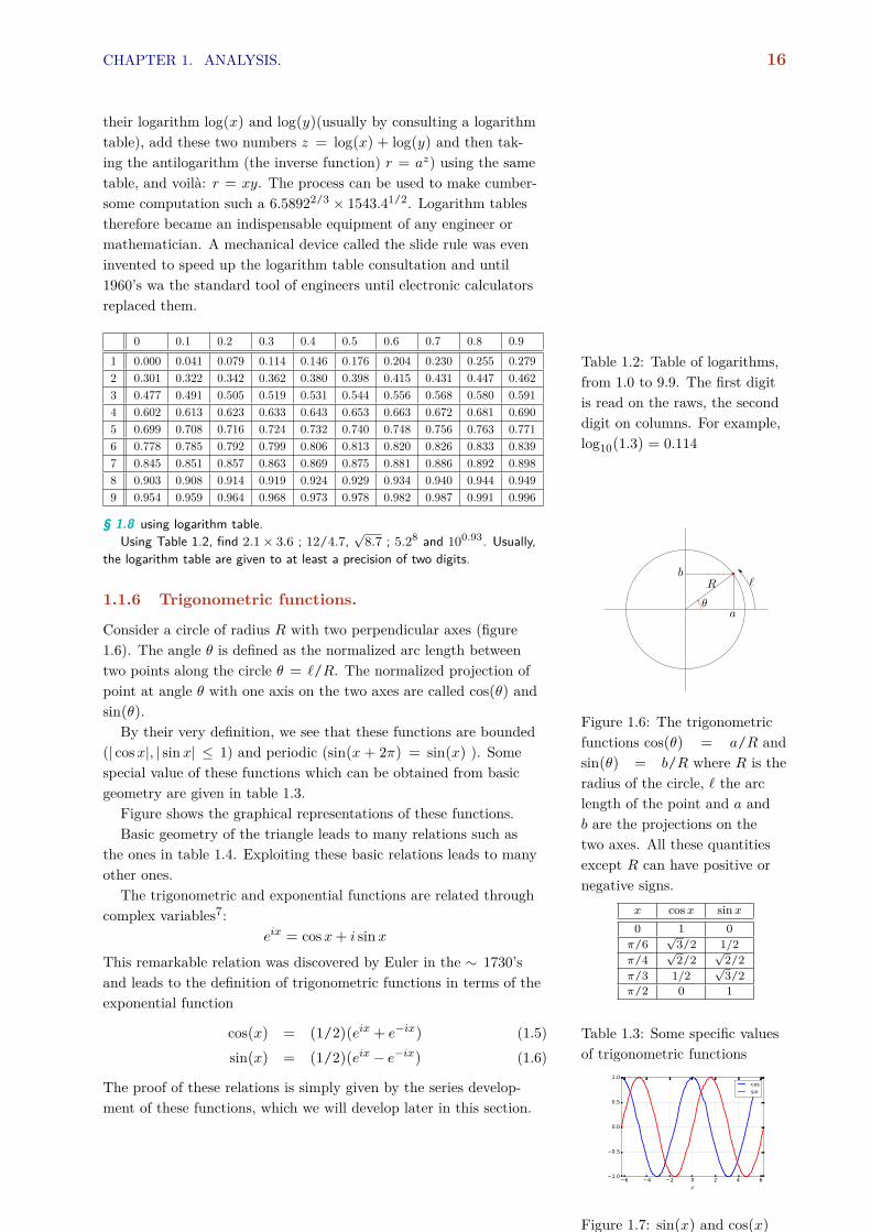
CHAPTER 1. ANALYSIS. 42
with three columns, where the arguments of the first column areindexed by x, the second column by y and the third column by z.We can for example write z = f(x) or z = g(y) or y = u(x) (figure1.28). We suppose u(.) to be strictly monotonic (see definition 4).
Figure 1.28: composed functionf = g u
We can construct two different integrals by infinitesimally sam-pling the interval [a, b]:
S1 =
ˆ b
af(x)dx =
N−1∑i=0
zi (xi+1 − xi)
S2 =
ˆ u(b)
u(a)g(y)dy =
N−1∑i=0
zi (yi+1 − yi)
Obviously, these two quantities are different S1 6= S2: even thoughthe zi is the same in the two sums for each i, its multiplicative factoris different in each case. For S1, it is the sample size in the first col-umn (xi+1 − xi) ; For S2, it is the sample size in the second column(yi+1 − yi). However, consider
S3 =
ˆ b
af(x)u′(x)dx =
N−1∑i=0
zi(xi+1 − xi)(yi+1 − yi)(xi+1 − xi)
We see that the addition of the correction factor at each step redressthe situation and this time we have indeed S3 = S2.
Theorem 7 Let f(x) = g (u(x)) where u(.) is a strictly monotonicfunction. Consider the intervals [a, b] and [ya, yb] where ya = u(a)
and yb = u(b). Thenˆ yb
ya
g(y)dy =
ˆ b
af(x)u′(x)dx (1.35)
This is an incredibly powerful tool to compute integrals. Like abazooka however, it gets some (correction:much) training to use itefficiently. Let us see some example.
§ 1.83 Develop a graphical interpretation of variable change in integrals.
The process of changing variable can be more automatized byusing efficiently the symbols dx and dy. Consider again the integralˆ yb
ya
g(y)dy
Now, set y = u(x) and therefore dy = u′(x)dx. In the above integral,whenever we see y, we replace it by u(x) and whenever we see dy,we replace it by u′(x)dx. Finally, for the boundaries, we must find asuch that u(a) = ya (in other words, a = u−1(ya).
Principle 1 The 3 steps workoutTo compute S =
´ ybyag(y)dy
1. Set y = u(x)
2. Set dy = u′(x)dx
3. Compute a = u−1(ya) andb = u−1(yb)
Example 1.15 Most important!Consider
S =
ˆ yb
ya
g(αy+ β)dy
Let us consider the function y = (x − β)/α. We have dy =
(1/α)dx. We can write S as
S =
ˆ αyb+β
αya+βg(x)
1αdx

43 1.7. THE CONCEPT OF INTEGRATION.
Note that the change of variable was suggested by the form ofthe argument. We indeed set directly x = αy + β, and thereforedx = αdy and we reversed this last relation.
For example, considerˆ π/2
0sin(2x)dx
we set y = 2x, dy = 2dx or dx = dy/2. On the other hand, whenx = 0 y = 0 and when x = π/2, y = π. So we have
ˆ π/2
0sin(2x)dx = (1/2)
ˆ π
0sin(y)dy = 1
Example 1.16 We can compute S =´ π/2
0 sin(2x)dx by anotherchange of variable. Note that sin(2x) = 2 sin(x) cos(x). Now, in
2ˆ π/2
0sin(x) cosxdx
Let us set y = sin(x) and dy = cos(x)dx ; when x = 0 y = 0 andwhen x = π/2, y = 1 so we have
S = 2ˆ 1
0ydy = 1
Example 1.17
I =
ˆ K
0
xdx
2x2 + 1
The form of the denominator suggests the change y = 2x2 + 1and dy = 4xdx. The numerator can be therefore written as dy/4.When x = 0 y = 1 and for x = K, we have y = 2K2 + 1 so
I =14
ˆ 2K2+1
1
dy
y=
14 [log y]2K
2+11
Example 1.18
I =
ˆ 1
0
dx
x2 + 1
Let us set x = tan θ and dx = (1 + tan2 θ)dθ. When x = 0,θ = 0 and when x = 1, θ = π/4 So
I =
ˆ π/4
0dθ = π/4
1.7.7 Integration by part.
The rule of derivative of the product of two functions can be writtenas
f ′(x)g(x) = (f(x)g(x))′ − f(x)g′(x)
Integrating the above relation, we obtain a relation called “integra-tion by part”:
ˆ b
af ′(x)g(x)dx = [f(x)g(x)]ba −
ˆ b
af(x)g′(x)dx

CHAPTER 1. ANALYSIS. 44
And of course, the same relation is obtained for indefinite integrals(primitives):
ˆf ′(x)g(x)dx = f(x)g(x)−
ˆf(x)g′(x)dx
The same relation is often writtenˆUdV = UV −
ˆV dU
where dV = f ′(x)dx and U = g(x) from which we get V = f(x) anddU = g′(x)dx.
These relations allow us to compute some interesting integrals .
Example 1.19 logTo compute
´log xdx, let us choose U = log x and dV = dx :
ˆlog xdx = x log x−
ˆdx = x log x− x
Example 1.20 polynomials and trigonometric.To compute
´x sin(x)dx , we need to get rid of the polynomial.
So we choose U = x and dV = sin(x)dx:ˆx sin(x)dx = −x cos(x) +
ˆcosxdx = −x cos(x) + sin(x)

45 1.8. EXERCISES: INTEGRATIONS.
1.8 Exercises: integrations.
§ 1.84 Consider the sum
Figure 1.29:∑Ni=1 f(i) − f(i −
1) = f(N)− f(0)
R2 =
N∑i=1
i2 − (i− 1)2
Show that R2 = N2. By expanding the parenthesis, deduce then that
Q1 =
N∑i=1
i = N(N + 1)/2
§ 1.85 Direct Computation of´xndx
Consider the sum
R3 =
N∑i=1
i3 − (i− 1)3
Show that R3 = N3. By expanding the parenthesis, deduce then that
R3 = 3Q2 − 3Q+N
where Q2 =∑Ni=1 i
2. Conclude by showing thatˆ b
0x2dx =
13x
3
Generalize the method to show that in generalˆ b
0xndx =
1nbn+1
§ 1.86 Direct Computation of´
sin(x)dxConsider the sum
I =
N∑i=1
sin(i.dx)
where dx = L/N . Recall that
2 sin a sin b = cos(a− b)− cos(a+ b)
and demonstrate, using figure 1.29, that
I sin(dx
2
)= cos
((i− 1
2 )dx)− cos
((i+
12 )dx
)Use this result to show that
ˆ L
0sin(x)dx = 1− cosL
§ 1.87 area of a circleWe know that the perimeter of circle of radius r is 2πr. This is in fact
the definition of the number π. What is its area ? The original proof of thearea of a circle comes from inscribing and circumscribing the circle by aregular N−polygon and then let N become large (taking the limit N → ∞).Demonstrate that this leads to the famous formula
Figure 1.30: Area of a circle byunwrapping.
S =12πr
2 (1.36)
Another method is to consider the circle as an onion, i.e. a collection of Ncircular stripes of width dr = r/N . Now peel them and superpose them.If dr is small, the unwrapped stripes now form a triangle of height 2πr (theperimeter of the outer stripes ) and height r = Ndr. We can now use theformula for the area of the triangle (one half of base multiplied by height) tofind relation (1.36).

CHAPTER 1. ANALYSIS. 46
§ 1.88 A surface of revolution is obtained by rotating a curve around an axis(figure 1.31). A cylinder and a cone for example are obtained by rotating astraight piece of line around an axis. For the first case, the line is parallel tothe axis, in the second case the line makes an angle with the axis. Let r(x)be the distance between the curve and the axis for a position x along the axis.The volume of the object is defined by
Figure 1.31: A surface of revo-lution, obtained by rotating acurve C around an axis.
V =
ˆ H
0πr2(x)dx
Demonstrate that for a cylinder of radius R, the volume is given by πR2Hwhile for the cone of the same radius, the volume is given by πR2H/3.
§ 1.89 If two objects of revolution have the same section at every height,they have the same volume. Consider a half sphere of radius R and a cylinderof the same radius and height R from which we have extracted a cone asshown in figure. Archimedes used a reasoning close to what we are doinghere. Demonstrate that the volume of the sphere is given by
Figure 1.32: Sphere’s volumeV = (4/3)πR3
§ 1.90 Develop a graphical interpretation of variable change in integrals.
§ 1.91 AreaThe equation for the upper half of the unit circle is given by
y =√
1− x2
Demonstrate that the area of the unit circle is π.
Figure 1.33: Ellipse
The equation for an ellipse is
y = b√
1− x2/a2
where a, b are the semi-length of the principle axes. Show that the area of theellipse is
A = πab
§ 1.92 trigonometricUsing the trigonometric relations cos2 x = (cos(2x) + 1) /2 and sin2(x) =
(1− cos(2x)) /2, computeˆ
cos2 xdx ;ˆ
sin2 xdx
§ 1.93 trigonometric 2Noting that cos3 x = cos2 x cosx, computeˆ
cos3 xdx ;ˆ
sin3 xdx
§ 1.94 Computeˆ √1− x2dx ;
ˆx√
1− x2dx ; ;ˆ
x√1− x2
dx
Try x = sinu as a change of variable. Then, for the last two primitives, trythe change of variable u = 1− x2. Do you obtain the same result ? Can youcompute the first primitive by the same change of variable ?
§ 1.95 Compute ˆdx
1 + x2 ;ˆ
xdx
1 + x2 ;ˆ
dx
x(1 + x2);
Try x = tanu as a change of variable. You could recall the trigonometricrelation 1 + tan2 x = 1/ cos2 x. For the second integral, use an other changeof variable u = 1 + x2.

47 1.8. EXERCISES: INTEGRATIONS.
§ 1.96 Change of Variable.Find the primitive of the following functions. 1/1 + 4x2 ; x/(2 + x)
; x(1 + x)1/3; x2√x+ 1 ; sin(cos(x)) sin(x) ; sin(√x)/√x ; log x/x ;
(log x)n /x ; x exp(−x2) ; x exp(−x2/2σ2) ; 1/√a2 − x2 ;
√a2 − b2x2 ;
x/√a2 − x2/c2 ; x
√a2 − x2; (a− bx2)/
√1− x2 ; sin x/ cos2 x ; sin(2x)/ cos4(x)
; cos(2x)√
2− sin(2x) ; (1 + x+ x2)/(a2 + b2x2)
§ 1.97 Second order rational.IShow that 1
1− u2 =12
( 11− u +
11 + u
)And compute ˆ
dx
1− x2
Show that we can write
x2 + bx+ c = (x− x1)(x− x2) (1.37)
if x1 + x2 = −b and x1x2 = c ; x1,2 are obviously the root of the quadraticequation, as for x = x1,2 , both sides are equal to zero. Show that
1x2 + bx+ c
=1
x2 − x1
( 1x− x1
− 1x− x2
)Supposing that x1,2 ∈ R, compute
ˆdx
x2 + bx+ c;ˆ
dx+ e
x2 + bx+ cdx ;
ˆx2 + dx+ e
x2 + bx+ cdx
§ 1.98 Second order rational.IIShow that if the roots of the polynomial x2 + bx+ c are complex, we can
write it asx2 + bx+ c = A+ (x−B)2
where you express A,B as a function of the coefficients b, c. Use this decom-position to compute
ˆdx
x2 + bx+ c;ˆ
dx+ e
x2 + bx+ cdx ;
ˆx2 + dx+ e
x2 + bx+ cdx
§ 1.99 Logarithm function.We can define the logarithm function by 1 x
u
0
1
2
3
4
5
1/u
Figure 1.34: The logarithmfunction is defined by the areabelow the curve 1/u, from 1 tox.
log(x) =ˆ x
1
du
u
Using this definition and change of variable, show that
log(1/x) = − log(x); log(xy) = log(x) + log(y); log(xα) = α log(x)
§ 1.100 Integration by part.Find the primitive of the following functions. x2 sin x ; xn log x ; xex;x2ex.
§ 1.101 Power of sin.Using IbP, show thatˆ
sinn xdx = − sinn−1 x cosx+ (n− 1)ˆ
sinn−2 x. cos2 x.dx
and then, by using cos2 x = 1− sin2 x, show thatˆ
sinn xdx = − 1n
sinn−1 x cosx+ n− 1n
ˆsinn−2 x.dx
Use this result to show thatˆ π/2
0sin2 xdx = π/4 ;
ˆ π/2
0sin4 xdx = 3π/16

CHAPTER 1. ANALYSIS. 48
§ 1.102 Using IbP, show thatˆ a
0(a2 − x2)ndx =
2n2n+ 1a
2ˆ a
0(a2 − x2)n−1dx
Compute the above expression for n = 3.
§ 1.103 The Γ(z) function.Consider the function defined by an integral
0 2 4 6 80.0
0.5
1.0z=1
0 2 4 6 80.0
0.5
1.0z=2
0 2 4 6 8t
0.0
0.5
1.0z=3
Figure 1.35: Functions tz−1e−t
for various values of z. Thearea below each curve representΓ(z).
Γ(z) =ˆ ∞
0tz−1e−tdt
called the “Gamma” function (figure 1.35). Show That Γ(1) = 1. Using IbP,show that
Γ(z + 1) = zΓ(z)
and conclude that for integers n, Γ(n+ 1) = n!. Knowing thatˆ ∞
0e−x
2dx =
√π/2
demonstrate that Γ(1/2) =√π. Find the general expression for Γ(n+ 1/2)
where n ∈N.
1.9 Application of infinitesimal calculus.
If integrals and differentials have become so widespread and usedin every area of physics and mathematics, it is because it allows foreasily computing problems that were otherwise insoluble or hardlysoluble. The principle is the following : Suppose that you know theanswer to a simple problem ; then you can answer a generalizationof this problem by cutting the inputs into (huge number of) smallsimple problems, compute the answer for each simple problem andthe sum up all the answers. Integration is the process of summingup.
Let us do some examples.
Example 1.21 Center of gravity,moment of inertia 1D.Let us suppose that we have to point masses along a one-
dimensional line : mass m1 at position x1 and mass m2 at po-sition x2. Their center of mass is at position
xG =m1x1 +m2x2m1 +m2
(1.38)
If you think in terms of a lever, this is the position of the fixedpoint that guaranties equilibrium. If you have N masses, theabove formula generalizes to
xG =N∑i=1
mixi/N∑i=1
mi (1.39)
Now, a point mass does not exist, all masses are distributedwith a local density of a mass ρ(x). For a distributed mass be-tween a and b, relation (1.39) becomes
xG =
ˆ b
axρ(x)dx/
ˆ b
aρ(x)dx

49 1.9. APPLICATION OF INFINITESIMAL CALCULUS.
by the very definition of integral.By the same token, in discrete form, the moment of inertia15 15 The moment of inertia plays the
role of mass in rotation problems.Mass alone is the “resistance” tolinear acceleration ; moment of in-ertia is the resistance to rotationacceleration.
around a point at position p (in one dimension) is
I =∑
(xi − p)2mi
and it immediately generalizes, for a distributed mass, into
I =
ˆ b
a(x− p)2ρ(x)dx
Example 1.22 Debit of a current.
Example 1.23 Elasticity.
Example 1.24 Electrostatic field.
Example 1.25 Navier-Stockes.
1.9.1

CHAPTER 1. ANALYSIS. 50
1.10 Approximating functions : Taylor expansion.
1.10.1 Revisiting the differential.
We saw that from a function f(.),we can build a new function f ′(.)such that at each point x, for h→ 0
f ′(x) =1h(f(x+ h)− f(x)) (1.40)
When we use the relation (1.40) in the abstract, mathematical sens,it does not matter if h is positive or negative, the result is the same.Numerically however the result can be slightly different if the sam-pling size is not too small. A better numerical method would be touse a symmetric relation such as, when h→ 0
f ′(x) =1
2h (f(x+ h)− f(x− h)) (1.41)
We can continue the derivation game and from the function f ′(.),build a new function f ′′(.) by the same process. It is however worth-while to see what the second derivative means in terms of the origi-nal function f(). By (the symmetric) definition
f ′′(x) =1
2h(f ′(x+ h)− f ′(x− h)
)=
14h2 (f(x+ 2h)− f(x)− f(x) + f(x− 2h))
=1
4h2 (f(x+ 2h)− 2f(x) + f(x− 2h))
or even better, if we normalize our sampling size h→ h/2,
Figure 1.36: The mean-ing of the second derivativef ′′(x) = d2y/dx2. The valueof the function at the point x iscompared to (subtracted from)the average of the value of thefunction at two neighboringpoints x ± h: d2y designatesthis difference and has to be di-vided (normalized) by dx2 = h2
to yield a finite quantity. Theconvexity of the function f() atx is determined by the sign ofthe second derivative.
f ′′(x) =1h2 (f(x+ h)− 2f(x) + f(x− h)) (1.42)
The quantity f(x+ h) + f(x− h) (see figure 1.36) is twice the aver-age of the two neighboring points of x, and this average is comparedto twice the value of the function at the point x. If the first one islarger, the function is positive convex, if it is smaller, the function isnegative convex ; if they are both equal, then at point x, the func-tion is similar to a line.
1.10.2 Taylor approximation.
Let us now come back to our original aim of approximating functionswhich led us in sections §1.3 and §1.5 to the concept of differenti-ation as the first order approximation : for a function f(.) and apoint x, given a small increment h we have
f(x+ h) = f(x) + f ′(x)h+ o(h) (1.43)
where the coefficient f ′(x), called the derivative, was computed forvarious functions such as f(x) = xα. Can we do better than thisapproximation ? For example, can we go to second order in h:
f(x+ h) = f(x) + f ′(x)h+C(x)h2 + o(h2)

51 1.10. APPROXIMATING FUNCTIONS : TAYLOR EXPANSION.
where the coefficient C(x) has to be determined ? The answer isyes, the coefficient C(x) = f”(x)/2 and we can indeed generalizethis approximation to any order we want, provided that f() can bederived to the desired order at point x :
−1 0 1 2 3
x−1.5
−1.0
−0.5
0.0
0.5
1.0
1.5cos(x)T1(x)T2(x)T3(x)
Figure 1.37: Taylor expansionof the function cos(x) aroundthe fixed point a = π/4. Tn(x)designate the order of the ap-proximation.
f(x+ h) =N∑n=0
1n!f (n)(x)hn + o(hN )
To see why this is indeed the case, let us go back to our first orderapproximation (relation 1.43) and see why the remaining error iso(h). Let us call the error, i.e. what we want to neglect, E1(h) :
f(x+ h) = f(x) + f ′(x)h+E1(h)
As we now know all the tricks of integration by part, we can showthat
E1(h) =
ˆ x+h
x(x+ h− u)f”(u)du (1.44)
Relation (1.44) is exact without any approximation yet. But express-ing the error as an integral allows us to evaluate its weight. Let ussuppose that f”(u) is bounded in the interval [x,x+ h] :∣∣f ′′(u)∣∣ < C
then the error is bounded by
|E1(h)| < C
ˆ x+h
x(x+ h− u)du =
C
2 h2
We see here that E1(h) weights at best as h2; in particular, E1(h)/h→0 when h→ 0 and therefore relation (1.43) is correct. Now, it is easyto generalize and show that
EN (h) = f(x+h)−N∑n=0
1n!f (n)(x)hn =
ˆ x+h
x(x+h−u)Nf (N+1)(u)du
and estimate that the error is at best of order N + 1. This is thebasis for Taylor expansion around a fixed point x.
Theorem 8 Taylor ExpansionIf a function f(.) possess N derivatives at a point x, then it can
be approximated by a N degree polynomials around the point.Namely,
f(x+ h) = a0 + a1h+ a2h2 + ...aNhN + o(hN )
where the coefficients are given by
an =1n!f (n)(x)
If the function is infinitely derivable at x, the infinite order polyno-mial is called the Taylor series of the function at point x.
Note that we can rename the terms and write the Taylor expan-sion as (figure 1.37).
f(x) = f(a) + f ′(a)(x− a) + 12f′′(a)(x− a)2 + ...

CHAPTER 1. ANALYSIS. 52
1.11 Exercises : Taylor expansion.
§ 1.104 Find second order approximations of√
4.2 and 3√1.1. Find thirdorder approximation for log(1.5). Compare the results to exact values.
§ 1.105 Consider two functions f() and g() such that
f(0) = 0; f ′(0) = 1; f”(0) = 0; f ′′′(0) = −1; repeat...
andg(0) = 1; g′(0) = 0; f”(0) = −1; f ′′′(0) = 0; repeat...
write the Taylor expansion of these functions ; supposing that we can derivethe Taylor series, show that for any x, f ′(x) = g(x) and g′(x) = −f(x).
Find a third order polynomials approximating cos(x) arounda = π/3.
§ 1.106
§ 1.107 Derive the Taylor expansion, around 0, of the functions1. ex;2. log(1 + x);3. sin(x), cos(x);4. 1/(1 + x) (you can use the binomial expansion)
§ 1.108 By integrating all terms of the Taylor series of 1/(1 + x), find theTaylor series of log(1 + x)
§ 1.109 Find the Taylor series of the complex function eix. By identifying itscomplex and imaginary parts, find the Taylor series of sin x and cosx.

53 1.12. APPENDIX.
1.12 Appendix.
1.12.1 manipulating the symbol∑.
It is important to be familiar with the symbolm∑i=n
f(i) (1.45)
which is a shorthand for long sums. For example, instead of writing
1 + 3 + 5 + 7 + 9 + 11 + 13
we can just write16 16 This is similar to the concept ofloop in computer languages.6∑
i=02i+ 1
The rule for the expression (1.45) is the following. i is called theindex of summation, n and m are the lower and upper boundariesof the sum. We begin by setting i = n, i.e. begin with the lowerboundary and write therefore f(n). Then, we increment i by settingi = n+ 1, computing the operand f(i) for this value of i and addit to what we previously had : f(n) + f(n+ 1). We continue thisoperation until the index i reaches the upper boundary m :
m∑i=n
f(i) = f(n) + f(n+ 1) + ... + f(m)
It is important to note that i can be called whatever we want, itsname does not change the meaning of the sum and if we explicit thesum as we did, we should never find the index.
§ 1.110 Write explicitly∑8i=4 i
2;∑4i=0(i + 4)2;
∑+4i=−4 sin(2πi/L) ;∑10
i=1 i2 − (i− 1)2
§ 1.111 Show thatm∑i=n
f(i) =
m−k∑i=n−k
f(i+ k)
§ 1.112 linearityShow that
S∑q=R
af(i) + bg(i) = a
S∑q=R
f(i) + b
S∑q=R
g(i)
§ 1.113 Show thatm−1∑i=n
f(i+ 1)− f(i) = f(m)− f(n)
Use this relation to show thatn∑i=1
i = n(n+ 1)/2
Hint: Study the sumn∑i=1
(i+ 1)2 − i2

CHAPTER 1. ANALYSIS. 54
§ 1.114 Study the sumn∑i=1
(i+ 1)3 − i3
and show thatn∑i=1
i2 =16n(n+ 1)(2n+ 1)
1.12.2 The Euler number e.
In subsection §1.1.5, we mentioned that the number e plays an im-portant role in analysis ; later on, we saw that the function ex isinvariant under derivation, (ex)′ = ex. How did Euler come uponthis very precious number ?
Consider the function ax and its approximation in terms of itsTaylor series
ax = B0 +B1x+B2x2 +B3x
3 +B4x4 + . . .
which we suppose valid for a range of x around 0 to be determinedlater. Let us first note that a0 = 1 so we must have B0 = 1. Obvi-ously,
a2x = 1 + 2B1x+ 4B2x2 + 8B3x
3 + 16B4x4 + . . .
On the other hand, a2x = (ax)2 so
a2x = 1 + 2B1x
+ (B21 + 2B2)x
2 + (2B1B2 + 2B3)x3
+ (2B4 + 2B1B3 +B22)x
4 + ...
Equating the two series term by term, we find that (i)
4B2 = B21 + 2B2
which implies that B2 = (1/2)B21 ; (ii)
8B3 = 2B1B2 + 2B3
which implies that B3 = (1/2× 3)B31 ; (iii)
16B4 = 2B4 + 2B1B3 +B22
which implies that B4 = (1/2× 3× 4)B41 . Continuing the recur-
rence, it is straightforward to show that
Bn =1n!Bn1
and therefore, the series can be written as
ax =∞∑n=0
1n!(B1x)
n
We still don’t know the value of B1, we only know that it dependson a, i.e. B1 = B1(a).

55 1.12. APPENDIX.
Let us call e the value of a which gives B1 = 1. We then have
e =∞∑n=0
1n!
= 1 + 1 + 12 +
12× 3 +
12× 3× 4 + ... (1.46)
Considering the first three terms of the series, it is obvious thate > 2. On the other hand, consider the geometric series
S = 1 + 12 +
14 +
18 + ... 1
2n + ...
Multiplying the series by 2, we realize that 2S = 2 + S and thereforeS = 2. Now compare the series giving e with the series 1 + S:
e = 1 + 1 + 12 +
12× 3 +
12× 3× 4 + ... 1
n!+ ...
3 = 1 + 1 + 12 +
12× 2 +
12× 2× 2 + ... 1
2n + ..
As n! > 2n for n > 2, each term in the expansion of e is smallerthan the corresponding term in the expansion of 3: we conclude thate < 3. So we know that
2 < e < 3
The expansion of e is a fast converging series. Calling eR the valueobtained by the first R terms of e’s expansion, we have
e1 = 2e2 = 2.5e4 = 2.70833e8 = 2.71828e16 = 2.71828
So we can compute e up to five decimal by taking only the first 8terms of the series. This is the computation done by Euler in the~1720’s.


Chapter 2
Differential equations.
Contents
2.1 A tale of treasure Island. 58
2.2 Linear first order equation. 59
2.2.1 Arithmetic approach. 59
2.2.2 Generalization. 60
2.2.3 Geometrical approach. 60
2.2.4 Analytical solutions of first order linear ODE. 61
2.2.5 Inverse function approach. 62
2.2.6 Separation of variables. 63
2.2.7 Non-homogeneous linear ODE-1. 64
2.2.8 Complex variables. 64
2.2.9 General first order equations. 66
2.3 Exercises: First Order equations. 67
2.4 Linear second order differential equation. 70
2.4.1 Decomposition into two ODE-1. 70
2.4.2 Non-homogeneous equations. 71
2.4.3 General second order equations: The Wronskian. 72
2.5 Solving a system of ODEs. 73
2.5.1 Singular Linear ODE of ∂2. 74
2.6 Numerical solution of ODE. 74
2.7 Exercises. 74

CHAPTER 2. DIFFERENTIAL EQUATIONS. 58
2.1 A tale of treasure Island.
You are in the possession of an Island map and a set of instructionto seek a treasure:
Figure 2.1: The map of thetreasure island.
Land on the south shore. From there, walk 100 steps where foreach 10 steps toward the north, you make one step toward the east.Then, walk 200 steps where for each 5 steps toward the north, youmake one step toward the west. Then, walk 128 steps where for eachstep toward the north, you make one step toward the west. Dig.Enjoy.
This set of instructions seems to be precise enough to guide yourpath. The navigation part contains two important information: (i)the initial point (the south shore); (ii) the set of instructions toguide your steps. Both information are necessary/mandatory toreach the treasure. Note that you don’t have to make the actualsteps. You can predict where the treasure is directly on the map.
These kind of instructions govern the whole natural world and arecalled differential equations. They are stated generally as
y(x = x0) = y0 (2.1)dy = f(x, y)dx (2.2)
The first line is the initial condition, similar to the south shore land-ing of the tale. The second line is the navigation instruction : foreach dx going east, go dy toward the north; The relation between thetwo is determined by f(x, y), where you are presently .
The history of differential equations goes back to around 1680,when humans learned the language of Nature. Suddenly, complicatedphenomena, the movement of objects, the shape of curves, the flowof heat, ... could be stated in a precise language and be predicted.This language is called differential equations and relates the rate ofchange of a quantity to the value of this quantity, through a givenrelation, as in the tale. The quantities can be anything, not onlypositions.
Example 1: Consider the geometric curve of a spiral and its curva-ture at some point. We can describe the spiral by relating the rateof change of the curvature at some point to the value of the cur-vature at this point: When going from P to P ′ along the curve,the relation dκ/ds = aκ would define a spiral, where κ is the cur-vature, ds is the arc length between P and P ′ and a a constant.We can give such a description to all curves ; this kind of curvedescription is called its intrinsic description.
Example 2: Consider a bucket with a whole at the bottom gettingemptied. If h(t) is the height of the liquid at time t, then the rateof change of the height is proportional to the height: dh/dt =
−ah
Example 3: let call x the position of a particle and v = dx/dt itsspeed. The particle is submitted to a force F which depends in

59 2.2. LINEAR FIRST ORDER EQUATION.
general on the position of the particle and its speed. The funda-mental equation of motion states that the rate of change of thespeed is proportional to the force (the proportionality constant isrelated to the mass):
mdv/dt = F(x, v)
Example 4: Consider a simple chemical equation A + B → C.The rate of change of the number of A molecules depends on thenumber of available A (and B) molecules : d[A]/dt = −k[A][B].As the reaction proceeds, the number of A molecules decreases, sothe rate of change is negative. On the other hand, as the numberof A decreases, the rate of change tends toward zero.
2.2 Linear first order equation.
2.2.1 Arithmetic approach.
As everything in the history of science, differential equations ap-peared as a normal extension of what people already knew, in thiscase in arithmetic. Consider a system of algebraic linear equation
y1 = (1 + α)y0
y2 = (1 + α)y1...
yN = (1 + α)yN−1
Stated like this, this is a system of N + 1 unknowns (y0, ...yN ) andonly N equation. The system is under determined: either we needto add one equation or to add the knowledge about one of the un-known. Let us suppose for the moment that we know y0. Then theabove system can be solved by successive substitution:
yN = (1 + α)Ny0
Now, consider the linear differential equation
dy
dx= ay (2.3)
which we want to solve on the interval [xA,xB ]. Let us discretize theproblem: if L = xB − xA, we define dx = L/N where N is a bignumber and set x0 = xA; x1 = x0 + dx ; xk = x0 + kdx. We don’tknow yet the function y(x), but we define yk = y(xk). Then fromwhat we know about differential, we can rewrite the equation (2.3)as
yk+1 − yk = a.dx.ykor alternatively
yk+1 = (1 + adx)yk
This is just the linear system we had before and its solution is obvi-ously
yk = (1 + adx)ky0

CHAPTER 2. DIFFERENTIAL EQUATIONS. 60
As dx is supposed to be infinitely small, we have
(1 + adx)k = ek log(1+adx) ≈ eakdx
Note that for x = kdx, the general solution of the ODE (2.3) is
y(x) = ekxy0
We observe that solving a first order ODE necessitates one initialcondition y(x0) = y0. Usually, given y0, the solution is unique.
2.2.2 Generalization.
What we did above can be generalized. An ODE-1 is just a simplerecurrence relation which we can formally solve, at least numerically.Consider the general ODE-1
Figure 2.2: Solving y′ = f(x, y)numerically over the interval[a, b]. The interval is sampledby dx, and xn = a + ndx.Knowing (x0, y0), we can findy1 = y0 + dx f(x0, y0). Oncey1 is determined, we can use itsvalue to find y2 and so on.
y′ = f(x, y) (2.4)y(a) = ya (2.5)
for x ∈ [a, b] where the function y(x) is unknown and we know theinitial condition y(a) = ya.
Let us discretize the interval [a, b] into small pieces xn = a+ nh
where h is the discretization size (sampling size), and we want todetermine yn = y(xn). In this discrete setting, equation (2.4) iswritten
yn+1 = yn + hf(xn, yn) (2.6)
so beginning with (x0, y0), we can find
h=0.01 # discretization stepb=4*pi # interval [0,b]x=0:h:b # vector xN=length(x)y=zeros(N) # create y vectory[1]=1.0 # initial valuefor i=1:N-1 # main loop to solve for y
y[i+1] = y[i]+h*f(x[i],y[i],alpha)end
Figure 2.3: A simple computercode to solve y′ = f(x, y) over[0, b], written in high level lan-guage “Julia”.
y1 = y0 + hf(x0, y0)
once we have found y1, we can find y2 and so one by the same recur-rence (figure 2.2). The method is called the Euler’s method (figure2.2 and 2.3).
Of course, for the method to work, the discretization step must besmall (see figure 2.4. How much small is a matter of great interest inapplied math, when the speed of resolution is of prime importance.But for ODE-1 and modern computer, numerical solution is a matterof few seconds at worst. We will see more efficient algorithms insection 2.6.
0 2 4 6 8 10 12 140
1
2
3
4
5
6
7
8
exactdx=0. 01
dx=0. 1
Figure 2.4: numerical solutionof y′ = y sin(x) for step sizedx = 0.01 and 0.1 and y(0) = 1solved by the above computercode. The exact solution isy(x) = exp(1− cosx).
2.2.3 Geometrical approach.
An equation of the typey′ = f(x, y) (2.7)
specifies the slope of the curve at each point in space : If the curvewe are looking for passes through the point (x, y), its slope at thispoint should be given by relation (2.7). So we can imagine the spacefilled with little “tangent” segment and then look for a curve with ateach of its point is tangent to these segments (figure 2.5). Obviously,

61 2.2. LINEAR FIRST ORDER EQUATION.
as figure 2.5 illustrates, there are infinitely many such curves ; aunique solution is obtained by requesting the curve to pass through afixed point (x0, y0).
1.0 1.2 1.4 1.6 1.8 2.0
x1.0
1.2
1.4
1.6
1.8
2.0
y
Figure 2.5: Solving a differen-tial equation by finding curves(in red) tangents to “slope seg-ments” (in black) in the plane.
Such geometrical visioning makes it also very intuitive to discussthe existence and unity of the solution, which we will study later.
2.2.4 Analytical solutions of first order linear ODE.
First order ODEs can, in general, be solved analytically. There aremany methods (tricks) to do that. As for integration, recognizingwhich method to use necessitates to recognize the general pattern ofthe equation.
In physics, the most current type of differential equation is thegeneral linear first order equation:
y′ − p(x)y = q(x) (2.8)
The following subsections contain the methods1 to solve this equa- 1 and the reason behind the method
tion and many more general ones. But as this equation is very im-portant, let us consider its solution first.
1. p(x) = a = Cte ; q(x) = 0 . This is called the linear ho-mogeneous first order equation with constant coefficient. Whenq(x) = 0, if some y(x) is solution of (2.8), then Ky(x) is also asolution, where K is a constant. This is why the equation is calledhomogeneous. The solution of this equation is trivially
y = y0 exp (ax)
2. q(x) = 0. The equation is still homogeneous, but the coefficient ofy is not constant any more. Let P (x) =
´p(x)dx, then it can be
checked that the solution is
y = C exp (P (x))
We can check this solution directly by deriving the above expres-sion:
y′ = P ′C exp (P (x)) = p(x)y
3. p(x) = a ; q(x) = b This time,both coefficients are constants.The equation is not homogeneous anymore. Note however thatfor ys = −b/a, we would have y′ = 0. This particular value ofy is called the stationary value : if y is at this point, it will staythere : y(x) = ys is a solution. Therefore, it is wise to measurethe deviation from this point by setting a new unknown functionu(x) = y(x)− ys or y(x) = u(x) + ys. Replacing y by u in (2.8)leads to
u′ − au = 0
which is the first case we have encountered. Once we have solvedfor u, it is trivial to come back to the original function y. This iscalled DC shift removal.

CHAPTER 2. DIFFERENTIAL EQUATIONS. 62
4. p(x) = a Here we don’t suppose anything about q(x). We knowthat if q(x) = 0, the solution is of the form y = C exp(ax).Similar to the previous case, we try to introduce a new unknownfunction to simplify the equation. This time however, instead ofmeasuring the deviation from the steady state, we measure the“multiplicative deviation” from the homogeneous solution, i.e. weset
y(x) = u(x)eax
Deriving and replacing y in the equation, we find
u′(x) = e−axq(x)
This is not a differential equation and need only a simple integra-tion:
u(x) =
ˆe−axq(x)dx+C
Once u(x) is found, it is easy to get back to y(x) by a simplemultiplications. The method, for historical reasons, is called “vari-ation of constants”, which seems to be an oxymoron.
5. Finally, for the most general case, we can combine the resultof items 2 and 4 : Let the solution of y′ − p(x)y = 0 be z(x),computable by the item 2 method. Then we look for the generalsolution of the form
y(x) = u(x)z(x)
where u(x) is a new unknown. Then, y′ = u′z + uz′ and
y′ − p(x)y = u′z + u(z′ − pz) = u′z = q
and we find the function u as before by a simple integration
u(x) =
ˆq(x)
z(x)dx
The items 1-5 cover the linear first order ODE. Let us now comeback to general first ODE equation of type
y′ = f(x, y)
and various ways of solving it.
2.2.5 Inverse function approach.
There are many ways to solve ∂1 equations, as we’ve seen above.The most natural one however is the inverse function method. Con-sider the simple relation
dy
dx= f(x) (2.9)
which is of course, not a differential equation. To get the functiony(x), we only need to do a simple integration
y(x)− y(a) =ˆ x
af(u)du

63 2.2. LINEAR FIRST ORDER EQUATION.
Now consider the differential equation
dy
dx= f(y)
if we consider the inverse function, i.e. use x as a function of y, wehave
dx
dy=
1f(y)
(2.10)
which has the exact same form than equation (2.9). Integrating overthe y variable, we have
x− a =
ˆ y
ya
du
f(u)
and once we know the function x(y), we can take the inverse func-tion and find y(x).
As an example, consider our old friend dy/dx = ay, with theinitial condition y(0) = 1. We have then
dx
dy=
1ay
; x =
ˆ y
1
du
au=
1a
log y
and taking the inverse function now gives us
y = eax
2.2.6 Separation of variables.
The inverse function method can be generalized as follow. Considerthe following ODE-1 over the interval [a, b]
y′ = f(x)g(y) (2.11)y(a) = ya (2.12)
which we can rewrite asdy
g(y)=
dx
f(x)
which we can integrateˆ y
ya
dv
g(v)=
ˆ x
a
du
f(u)
Computing the integral gives us the function y(x), at least in an im-plicit form. Very often, instead of using integrals, we use primitives,letting an unknown constant to be found later. For example, y′ = αy
can be written asdy/y = αdx
taking the primitive, we have
log y = αx+C
or y = C ′ exp(αx), where the constant C ′ is not yet known. Usingthe initial condition y(a) = ya determines C ′ = ya exp(−αa) and thefull solution can be then written as
y = yaeα(x−a)

CHAPTER 2. DIFFERENTIAL EQUATIONS. 64
2.2.7 Non-homogeneous linear ODE-1.
Consider the ODE-1y′ = αy+ f(x) (2.13)
over the interval [a, b] with the initial condition y(a) = ya whichoccur frequently in all kind of situation, such as in mechanics wherethe force applied to the particle depends on the position of the par-ticle and on time. We cannot solve this equation with separation ofvariables (why ?).
Note however that if f(x) = 0, the solution is simply exp(αx).We can try to compute the solution as compared to this function.Consider the solution as
y(x) = u(x)eαx (2.14)
where we have introduced a new unknown function u(x). We notethat
y′ = u′eαx + αu
and therefore replacing y by u in equation (2.13) produces
u′ = e−αxf(x)
But as you note, we can find here u by a simple integration
u(x) =
ˆe−αxf(x)dx+C
and the solution is therefore
y = Ceαx + eαxˆe−αxf(x)dx (2.15)
and the constant C can be find by using the initial condition.
2.2.8 Complex variables.
Everything we said above for linear ODEs generalizes to functions ofone real variable that are complex. For example, the equation
dz
dt= 2iz
has the solutionz = e2it
The general linear first order ODE
z′ − p(t)z = q(t)
can be solved without modification by the methods of subsection2.2.4(page 61). This is a consequence of linearity.
Let us consider again the complex equation
z′(t) = ηz

65 2.2. LINEAR FIRST ORDER EQUATION.
where η ∈ C. We can study the real and imaginary part of thisequation separately. Note z = x+ iy and η = α+ iβ. then
dx
dt= αx− βy (2.16)
dy
dt= βx+ αy (2.17)
which is a system of two ordinary ODEs. The general solution ofthese kind of systems is discussed below, but we see the relationbetween complex equations and system of equations.
On the other hand, if α = 0, we derive equation (65) we find
d2x
dt2= −β dy
dt= −β2x
or x′′ + β2x = 0. So, a complex first order ODE can be reduced twoa real second order ODE. These are indeed the general method weuse to solve second order ODEs by reducing them to first order one.

CHAPTER 2. DIFFERENTIAL EQUATIONS. 66
2.2.9 General first order equations.
A word on uniqueness, following Arnold argument on Lifshitz condi-tions.

67 2.3. EXERCISES: FIRST ORDER EQUATIONS.
2.3 Exercises: First Order equations.
First order linear equation.§ 2.1 fluid frictions
The friction force exerted on a body moving in a fluid (air, water, ...) isFfr = −ρv where v is the speed of the body and ρ the friction coefficientwhich depends on the viscosity of the fluid and the shape of the body. Usingthe Newton law of the motion
mdv
dt= F
where m is the mass of the object, find how the speed of the object varies asa function of time. For a friction coefficient of ρ = 1Kg/s, find how muchtime it take for a mass of 1g or 1000Kg to loose half its speed.
§ 2.2 radioactive decayThe decay rate of 235U is 10−9year−1. How much uranium disintegrates
over 1 year ? 1000 years ? 106 years ?
§ 2.3 ChemostatIn a chemostat, glucose concentration decreases (because of bacterial
consumption) with rate µ, but fresh nutriment is imported from the reservoirwith debit q. The differential equation for the glucose concentration c(t) as afunction of time is therefore
dc
dt= −µc+ q
1. Solve the above differential equation with initial concentration c(t = 0) =c0.
2. Find cs the stationary value of the concentration reached for long times.3. If c0 = 2cs, how much time does it take for the concentration to reach
1.5cs ?4. For numerical application, consider q = 1mM/min and µ = 0.025 min−1.5. Represent graphically the solution.
Note : The degradation is supposed to be proportional to the glucose con-centration because the number of bacteria consuming glucose is proportionalto glucose. However, it take some times for bacteria to change their numberwhen glucose concentration is changed, and a correct approach would be towrite two differential equation, one for glucose and one for bacteria, whichwould lead to a second order differential equation for c.
§ 2.4 free fall in fluid frictionsLet us come back to exercise 2.1 and consider a free fall in such a medium,
where in addition to the friction force −ρv, we have the gravitation force mgwhere g is a constant called the gravitation acceleration2. Find how the speed 2 g = 9.8m2/sof the object varies as a function of time and compute the limit speed as afunction of the mass, and the friction coefficient.
Inverse functions.§ 2.5 Lifshitz
solve the differential equation y′ = ayα on the interval [0,∞[, with theinitial condition y(0) = y0.
In particular, show that, for α < 1 there exist a value x1 such that forx > x1, y = 0. What could you conclude about the uniqueness of the solution?

CHAPTER 2. DIFFERENTIAL EQUATIONS. 68
§ 2.6 Solve y′ = ay2 + 1
§ 2.7 Solve y′ = 1/ cos y
§ 2.8 logistic equationIn a habitat, individuals duplicate at rate α and their number n should
vary asdn
dt= αn (2.18)
However, as their number grows, the available resources are depleted and thereproduction rate α fall down. Malthus propose to model the variation of α as
α = α0(1− n/K)
where α0 is the base rate and K is called the carrying capacity of the habitat.Solve equation (68) and study the two case n(t = 0) > K and n(t = 0) < K.
Separation of variables.§ 2.9 Solve y′ = α sin(x)y over [0, b], with y(0) = 1. (figure 2.4)
Solution. We have dy/y = α sin(x)dx or, when integrating,
y = Ce−α cos(x)
on the other hand, for x = 0, we have y = 1 which determines C and thecomplete solution is then
y = eα(1−cos(x))
0 1 2 30
1
2
3
4
y ′= −√y
y ′= y2
Figure 2.6: Solution ofy′ = −√y and y′ = y2 withy(0) = 1.
§ 2.10 Solve y′ = α√y with y(0) = 1.
Find, for α < 0, at which value of x the function becomes zero. How toextend the function beyond this point ? Is the solution unique ?
§ 2.11 Solve y′ = αy2 with y(0) = 1.Find, for α > 0, at which value of x the function becomes infinite. How to
extend the function beyond this point ?The above two exercises show that the solution of a differential equation
can become zero or infinite for finite x. This is radically different from thesimple linear differential equation y′ = αy. The idea in these two exerciseslead to the general principles of the uniqueness of the solution of a differentialequation.
§ 2.12 Solve y′ = a(x)y with y(0) = y0 in general. You can call A(x) theprimitive of a(x).
§ 2.13 ShapeA geometric curve obeys the ODE
dy
dx= −x
y
What is the nature of this curve ?
§ 2.14 Chemical reactionConsider the chemical reaction
A+A→ P
if we call x(t) the concentration of molecule A at time t, we have
dx
dt= −kx2
A chemical reaction takes place when two molecule of A encounter each otherand hence the probability for this event is proportional to the square of x.

69 2.3. EXERCISES: FIRST ORDER EQUATIONS.
This is why this equation has this form. Solve this equation, knowing that att = 0, x(0) = x0.
Study the kinetics ofA+B → P
For this, you have to note that each time a molecule of A is consumed, amolecule of B is also consumed. The difference between their concentrationremains constant.
Study the reaction
A+A → A2
A+A2 → A3
Non homogeneous equations.§ 2.15 Solve the linear equation
y′ = ωy +Ae−ωt
where y = y(t) is the unknown function and y(0) = y0.
Solution. we haveu′ = Ae−2ωt
and therefore u = −(A/2ω) exp(−2ωt) +C ; the solution is
y = ueωt = Ceωt − A
2ω e−ωt
§ 2.16 Chemostat IILet us study a chemostat problem again. The reproduction rate of bacteria
α depends on the concentration s of nutriment : α = α(s). Usually, it is ofthe form
α(s) = α0s
s0 + s
where α0 and s0 are two constants. The equation for the evolution of thenumber of bacteria n(t) and nutriment concentrations s are
dn
dt= α(s)n− φ
Vn
ds
dt= −α(s)n+ φ (sin − s)
where sin is the concentration of the nutriment in the fresh flow brought tothe chemostat.1. Justify/discuss the form of α(s)2. Justify/discuss the form of evolution equation.3. Find the stationary point of the chemostat and show how the number of
bacteria inside are simply controlled by the flow.

CHAPTER 2. DIFFERENTIAL EQUATIONS. 70
2.4 Linear second order differential equation.
We learned how to solve first order ODE; how can we use the resultto go beyond that ? After all, most of the physics is governed bysecond order differential equations. There is a deep link betweenlinear ODEs of any order and matrices, which we expose in the nextsubsection. However, for linear ODE-2, the solution can be obtainedby simpler mean.
2.4.1 Decomposition into two ODE-1.
As a first example, consider
y′′ − ω2y = 0 (2.19)
where the function y(x) is unknown. Let us set
u = y′ − ωy (2.20)
Of course we don’t know u(x) yet. But
u′ = y′′ − ωy′
= ω2y− ωy′
= −ω(y′ − ωy)= −ωu
Surprisingly, the differential equation governing u is a simple ODE-1! Its solution is u(x) = C exp(−ωu) where the constant C will bedetermined later. The equation (2.20) can now be written as
y′ = ωy+Ce−ωx
Which is just a linear ODE-1, but non-homogeneous. We know howto solve this equation (see §2.15) and the general solution is
y = C1eωx +C2e
−ωx
The method exposed above show that a linear ODE-2 can be de-composed into two linear ODE-1 which can be solved. Of course,this also means that we now need two initial condition to solve com-pletely the equation (determine C1 and C2).
The fundamental exercise below generalize the above method.
§ 2.17 Following the same line of argument, show that the general solution of
y′′ + by′ + cy = 0
isy = C1e
r1x +C2er2x
where r1,2 are the two roots of the algebraic equation
r2 + br+ c = 0 (2.21)
Solution. Let us setu = y′ − r1y

71 2.4. LINEAR SECOND ORDER DIFFERENTIAL EQUATION.
is one of the roots of the equation (2.21) (we suppose r1 6= r2). Then
u′ = −(b+ r1)y′ − cy
but b+ r1 = −r2 and r1r2 = c so
u′ = r2(y′ − r1y) = r2u
Therefore u = C exp(r2x),
y′ − r1y = Cer2x
and the solution, according to equation (2.15) is
y = C1er1x +C2e
r2x
§ 2.18 By using the above method, show that if r1 = r2 = r, the solution is
y = erx(C1x+C2)
As the reader is well aware of, the second order algebraic equation(2.21) may have complex roots if b2 − 4c < 0. Complex quantities arehandled exactly as real quantities (see chapter 3). For the exponen-tial, we can use the Euler’s formula
eiθ = cos(θ) + i sin(θ)
to express everything in terms of sine and cosine functions. However,it is more elegant and economical to stay with complex variables. Inparticular, the roots of equation (2.21) can be written as
r1,2 = ν ± iω
and the general solution as
y = eνx(C1e
iωx +C2e−iωx)
= eνx ((C1 +C2) cos(ωx) + i(C1 −C2) sin(ωx))
Note that if we began with a function y which was real, the solutionwe obtain must stay real at all x.
One important point we did not discuss is the case when the tworoots are equal r1 = r2.
In depth discussion of the solution, damping and oscillations.
2.4.2 Non-homogeneous equations.
Consider the equation
y′′ + by′ + cy = q(x) (2.22)
If q(x) = 0, we know how to solve this equation. Let us call thesolution in this case yh(x) (h for homogeneous). As we did is subsec-tion 2.2.4 for non-homogeneous first order equation, we look3 for the 3 This is a very general method for
linear equations of any order.solution of the formy(x) = u(x)yh(x)
where the function u(x) is unknown. Deriving two times, we find
y′ = uy′h + u′yh
y′′ = uy′′h + 2u′y′h + u′′yh
CHAPTER 2. DIFFERENTIAL EQUATIONS. 72
Replacing these relations into equation (2.22) and noting that y′′h +ay′h + byh = 0, we find
yhu′′ + (2y′h + byh)u
′ = q(x) (2.23)
If we look carefully, this is a first order linear ODE of the form
v′ − α(x)v = β(x)
where v = u′. To solve this equation, we use the methods of subsec-tion 2.2.4 .
A very important non-homogeneous equation is
y′′ + by′ + cy = A sin(ωx)
The variable y is submitted to an oscillatory excitation. This caseis covered in depth in the mechanics part of these lecture, throughexample ?? (see equation 6.16 on page 110).
2.4.3 General second order equations: The Wron-skian.
A general second order linear equation of the form
y′′ + b(x)y′ + c(x)y = 0 (2.24)
cannot be solved exactly in most cases. Specific cases appearing inphysics have been intensely investigated and their solutions haveusually acquired the name of their investigators (Jacobi, Hermit,Bessel, Airy,...). They are generally called special functions of mathe-matical physics. We are not going to dwell into this field.
However, we know that the general solution of equation (72) is acombination of two functions f(x) and g(x). If by some chance, youknow one of the solution, then you can find the other.
Suppose we know f(x). Consider the wronskian 4 4 Named after Wronski which intro-duced it around 1800.
w(x) = fg′ − f ′g (2.25)
Differentiating w, we find
w′ = fg′′ − f ′′g= f(−bg′ − cg)− g(−bf ′ − cf)= −b(fg′ − gf ′)
In other words,w′(x) + b(x)w(x) = 0
This is however just a first order equation we know how to solve.Once solve, we can rewrite equation (72) as
f(x)g′(x)− f ′(x)g(x) = w(x)
which is a first order linear equation in g(x), because we know bothf(x) and w(x). Therefore we can find g(x), the second independentsolution.
Application: chemical kinetics, enzymes, ...

73 2.5. SOLVING A SYSTEM OF ODES.
2.5 Solving a system of ODEs.
To read this section, you need to know the results of chapter 5 aboutlinear algebra.
Consider the second order ODE
y′′ + ay′ + by = 0 (2.26)
where y = y(x) and a, b are constants. Let us set z(x) = y′(x),i.e. introduce an unknown function defined by the derivative of theunknown function y. A priori, we have increased the number ofunknowns, but now, the equation (2.26) can be written as
d
dxy = z
d
dxz = −by− az
Now, if we define the vector |u〉 = (y, z)T and the matrix
A =
(0 1−b −a
)(2.27)
we see that the above linear system is simply
d
dx|u〉 = A |u〉 (2.28)
which is a vectorial first order ODE. But we know from our studiesin the first chapter that there is no big difference between scalar andvectorial systems, if we think in terms of eigenvalues and eigenvec-tors. In particular, the numerical solution by recurrence is exactlythe same as before.
The eigenvalues λ1,2 of the matrix A are given by the equation
λ2 + aλ+ b = 0 (2.29)
Note the similarity between the algebraic equation (2.29) and thedifferential equation (2.26): order of differentials are replaced bypowers. 5. We know that there exist a matrix X (formed of eigen- 5 This is of course no coincidence:
operators, which transforms functionsinto functions, form an algebra. Wecan equip an ensemble of objects byan algebra, provided we can definethe operations of addition and mul-tiplication. For operators, the mul-tiplication is defined by the rule ofcombination: O1O2(f ) = O1(O2(f )).So, if we define D = d/dx, we haveD2 = d2/dx2. Linear differen-tial equations inherit many of theproperties of classical algebra.
vectors of A) such thatAX = XΛ
Let us define a new vector |v〉 such that |u〉 = X |v〉. Let us sup-pose for the moment that X is reversible, then obviously, the linearequation (2.28) X(d/dx) |v〉 = AX |v〉 can be written as
d
dx|v〉 = Λ |v〉 (2.30)
by multiplying both sides by X−1. We’re done. Equation (2.30) istwo separate (decoupled) equations of the form
dv1dx
= λ1v1 ; dv2dx
= λ2v2
and thereforevi(x) = eλixvi(0)

CHAPTER 2. DIFFERENTIAL EQUATIONS. 74
So now, if we come back to the original equation in terms of ui andy, we see that the general solution for y must be of the form
y(x) = C1eλ1x +C2e
λ2x
where C1 and C2 are two coefficients to be determined from theinitial conditions.
Exercice 1: solve ...
Exercice 2: solve ...
Exercice 3: solve ...
We can write the above results quite generally. Let us define theexponential of the matrix Λ, which is of course a matrix itself,
U(x) = exΛ =
(eλ1x 0
0 eλ2x
)
then the general solution of equation (2.30) can be written as
|v(x)〉 = U(x) |v(0)〉
or, coming back to the vector |u〉,
|u(x)〉 = XU (x)X−1 |u(0〉 (2.31)
We can define the exponential of the matrix A by
exA = XexΛX−1
so the solution of the vectorial equation (2.28) is directly given by
|u(x)〉 = exA |u(0〉
which is a very natural and straightforward way of extending thescalar results we already know. The end of this chapter contains asection on the general concept of f(A), where f is a function (suchas sin or log) and A a matrix.
2.5.1 Singular Linear ODE of ∂2.
In the preceding subsection, we didn’t consider the case when oneeigenvalue is 0.
2.6 Numerical solution of ODE.
2.7 Exercises.
Problems from mechanics, electricity to prepare to what is coming.

Chapter 3
Complex numbers.
Consider a point P rotating around a center at constant angularspeed (figure 3.1). This means that the angle θ of the point with anaxis (say the x axis) is given by
θ(t) = ωt+ φ
where ω is called the angular speed (dimension T−1) and φ the phase(the angle at time t = 0 ). The distance of the point to the centerr, remains constant. The projection of the point on the two axes istherefore
Figure 3.1: A point P rotatingat constant angular speed ωarount a center at three dif-ferent times. The initial angle,called the phase is noted φhere.
x(t) = r cos(ωt+ φ)
y(t) = r sin(ωt+ φ)
On the other hand, we can make the reverse approach and considerany alternating quantity such as x(t) = r cos(ωt+ φ) as the pro-jection of a point in two dimension rotating at constant speed. Wedo this because rotations at constant speed are very easy to handlemathematically, specially if we use complex numbers. As alternatingphenomena appears through all the physical branches, we need toget familiar with these numbers
3.1 Numbers and algebra.
A collection E of objects with an algebra is called numbers. Theword “algebra” only means that for these objects, we are able to de-fine two operation of +(addition) and . (multiplication) in a coherentway. For example, consider the natural numbers N = 0, 1, 2, ...where we know how to define these operations : 2+3=5 and 2.3=6 .To be called an algebra, few other details are needed. We must havean element called 0 and an element called 1 which are neutral for ad-dition and product respectively : x+ 0 = x , x.1 = x. Furthermore,we also need the associativity: for x, y, z ∈ E
x.(y+ z) = xy+ xz
Natural numbers come equipped with an algebra, well known to thereader.

CHAPTER 3. COMPLEX NUMBERS. 76
§ 3.1 The element −x is defined such that x+ (−x) = 0. The left hand isusually noted x− x. By considering x(y− y), show that x.0 = 0.
We can create other numbers on top of the natural numbers. Forexample, consider couples of natural numbers q = (x, y), wherex, y ∈N. For these objects, let us define
q1 + q2 = (x1y2 + x2y1, y1y2)
q1q2 = (x1x2, y1y2)
and for these new objects, we can define a zero and a unity elements0 = (0, 1) and 1 = (1, 1). The reader can verify that these new ob-jects have a well defined algebra and can be called numbers. Usually,q = (x, y) is noted
q =x
y
These numbers are called rational numbers and their collection isnoted Q. We can further extend Q to create1 the ensemble of real 1 The operation of extension is called
closing, and uses the concept oflimits.
numbers noted R. The numbers in R can be associated to points onan axis (figure .
Figure 3.2: Real numbers canbe identified with points on anaxis.
3.2 Complex numbers.
We can also extend R by considering couples of real numbers z =
(x, y), x, y ∈ R. A possible algebra can be defined as
z1 + z2 = (x1 + x2, y1 + y2)
z1z2 = (x1x2 − y1y2,x1y2 + x2y1)
and the neutral elements of these numbers are 0 = (0, 0) and 1 =
(1, 0). The element (0, 1) is called i.
§ 3.2 Show that i2 = i.i = −1
These numbers are called complexes (for historical reason) andthey are usually noted z = x + iy. The notation allows one tonaturally perform algebraic operation, keeping in mind that i2 = −1.As each complex number is a collection of two real ones, we canidentify the number z with a point in a plane.
Figure 3.3: The complex num-ber z = x+ iy can be identifiedto a point in the plane, whoseprojection on the two orthog-onal axes are x and y. Thequantities z∗ and |z| are alsorepresented.
3.3 Usual Operations.
For z ∈ C, Re(z) and Im(z) represent its projection on the two axis:z = Re(z) + iIm(z). The quantity z∗, the complex conjugate of z, isdefined as
z∗ = Re(z)− iIm(z)
The module of z = x+ iy is defined as
|z| =√x2 + y2
and a small computation shows that
|z|2 = zz∗

77 3.4. APPLICATION TO FORCED HARMONIC OSCILLATOR.
All the algebraic operation defined on R naturally extend to C.For example, a polynomial is of the form
P (z) =N∑i=0
aizi
Specifically, we can define the function ez
ez =∞∑n=0
zn
n!
which naturally extends the definition of exponential function forreal variables. Around 1740, Euler realized that for θ ∈ R, the abovedefinition leads to2 2 The power series for exp(.) is (see
example ??)
ex =
∞∑i=0
xn
n!
If we accept that this series is alsovalid for complex number and writethe power series for exp(ix), weimmediately see that the real partof this power series corresponds tothe cos(x) power series, while itsimaginary part corresponds to tothe sin(x) power series. This is howEuler deduced its relation.
eiθ = cos(θ) + i sin(θ) (3.1)
Note that by its very definition,∣∣eiθ∣∣ = 1, so the number eiθ is
at angle θ with the x axis and resides on the unit circle. We seetherefore that any complex number z = x+ iy can also be written as
Figure 3.4: z = x + iy = reiθ
are two different representationof the same complex number.
z = reiθ
where r = |z|. The relation between these two notation is
x = r cos θ ; r2 = x2 + y2
y = r sin θ ; tan θ = y/x
Consider now the number eiα where α ∈ R. Multiplying a com-plex number z by eiα is equivalent to rotating its representativepoint by the angle α:
zeiα = reiθeiα = rei(θ+α)
So, an object rotating in the plane at constant angular speed ω canbe modelled by the complex number
z = rei(ωt+φ)
We see how easily complex numbers take care of rotations in theplane by just a trivial multiplication operation.
3.4 Application to forced harmonic oscillator.
Consider the ODE for forced harmonic oscillation (see Chapter 6 ,example ?? ):
d2x
dt2+ ν
dx
dt+ ω2
0x = a cos(ωt) (3.2)
we know that the solution is an oscillating one at frequency ω. Letus then “complexify” the above equation by considering x(t) as thereal part of complex variable z(t). By the same token, the righthand side would be a exp(iωt), so the complex version of equation(3.2) would be
d2z
dt2+ ν
dz
dt+ ω2
0z = a exp(iωt) (3.3)

CHAPTER 3. COMPLEX NUMBERS. 78
We see that taking the real part of equation (3.3) produces equation(3.2) ; we can thus do all our computations with z and take the realpart of z at the end to come back to x.
Considerz = z0e
iωt
as a solution, where z0 ∈ C. Plugging this expression into equation(3.3), we find
z0(−ω2 + iνω+ ω2
0)eiωt = aeiωt
and therefore the complex amplitude is
z0 =a
ω20 − ω2 + iνω
We see that all the cumbersome manipulation of sine and cosine isreduced to a simple algebraic operation. Furthermore, we can write
z0 =a
re−iφ
where
r2 =(ω2
0 − ω2)2 + (νω)2
tanφ =νω
ω20 − ω2
and the quantity x(t) = Re(z(t)) we were interested in in the firstplace is
x(t) =a
rcos(ωt− φ)
Compare this computation to example ?? to taste the beauty ofcomplex variables.
3.5 Exercises.
§ 3.3 circleShow that a circle of radius r centered at the origin is given in complex
representation byzz∗ = r2
What would be the equation of a circle centered around the point zA ?
§ 3.4 lineShow that the equation of a line is given by
z = P + ct
where P , c ∈ C and t ∈ R. Draw this line in Cartesian representation.Consider the line equation
z = P + (P ′ − P )t
where P ,P ′ ∈ C. What are the values of z for t = 0 and t = 1 ? Draw thisline.
§ 3.5 Circle power
Figure 3.5: Power of a pointwith respect to a circle of ra-dius r.
In plane geometry, the power of a point A in respect to a circle C of originO and radius r is defined as follow : draw a line from A which crosses the

79 3.5. EXERCISES.
circle at two point C1 and C2 (figure 3.5). The power of the point A inrespect to the circle C is then
pA = AC1.AC2 (3.4)
where AC1 and AC2 are the segments length. Using complex number, showthat pA does not depend on the line used to cross the circle, but only on thedistance of the point A from the origin O.
Solution. The equation of the circle is zz∗ = r2. The equation of theline going through the point A is z = A+ ct, where c ∈ C and t ∈ R (seepreceding exercises). The point Ci, the crossing of the line and the circlemust therefore obey the relation
(A+ ct)(A+ ct)∗ = r2
in other word, we must find the two roots t1 and t2 of the equation
(cc∗)t2 + (Ac∗ +A∗c)t+AA∗ − r2 = 0 (3.5)
to find the points Ci = A+ cti.Now, we have
p2A = (C1 −A)(C1 −A)∗(C2 −A)(C2 −A)∗
= (cc∗)t21(cc∗)t22
But from the second order algebraic equation (3.5) we have
t1t2 = (AA∗ − r2)/(cc∗)
and therefore, finally,p2A = AA∗ − r2
We see here that AA∗ is just the square of the distance of A to origin, andthe power of the point does not depend on the line we used to go trough thepoint A.
Note that the point A does not need to be inside the circle, all the abovecomputation generalize to any point.
§ 3.6 Geometric Inversion.Given an origin O, a point P ′ in the plane is said to be the geometric
inversion of a point P ifOP .OP ′ = 1
where OP and OP ′ are the length of the corresponding segments. Usingcomplex variables, show that the inversion of a line is a circle and that theinversion of a circle is a circle or a line.
Solution. Hint: show that the image of a point z is the point z′ = 1/z∗.Use this fact to make the demonstration, by for example considering theimage of the line
z = a+ it
For the case of the circle centered on a, whose equation is given by
(z − a)(z − a)∗ = r2
let us suppose without loss of generality that a ∈ R. The image of a point onthe circle is given by ζ = 1/z or z = 1/ζ. Therefore
(1ζ− a)( 1
ζ∗− a) = r2
or(a2 − r2)ζζ∗ − a(ζ + ζ∗) = −1

CHAPTER 3. COMPLEX NUMBERS. 80
which can be rearranged into
ζζ∗ − a
(a2 − r2)(ζ + ζ∗) +
a2
(a2 − r2)2 =r2
(a2 − r2)2
This is the equation of a circle centered en a/(a2− r2) with radius r/∣∣a2 − r2∣∣.
A line can be seen as a circle of infinite radius.

Chapter 4
The Fourier Series.
Contents
4.1 Definition. 82
4.2 The idea of basis in the function space. 82
4.3 Examples of Fourier series. 85
4.4 Sine and Cosine series. 85
4.5 Complex Fourier series. 86
4.6 The vibrating string. 87
4.7 Some other Orthogonal bases. 88
4.8 The Fourier Transform. 88

CHAPTER 4. THE FOURIER SERIES. 82
4.1 Definition.
The Fourier series are one of the main tools of mathematics used byphysicists. To us humans, the concept is a natural one, because thatis how we hear sounds: our ears transform the sound signal into itsFourier components and this is precisely why music is so dear to us.
The emergence of the field was however accompanied by somecontroversies1 when Fourier proposed it (~1810) as a tool to solve 1 As we’ll see later, the controversy
was about how summing continuousfunctions can produce discontinuousfunctions.
the vibrating string and the heat diffusion problem. The controversywas beneficial to mathematicians, as it helped them to shed light onthe concept of convergence and measure in general.
Definition 5 L1 functions.The conservative definition of
reasonable function f for Fourierseries is one for which
ˆ L
0|f(x)|dx
is finite (which we note by < ∞). We say that the function f(.) isL1 or belongs to the class of L1functions. We can slightly relax thisconstraint, but for our lecture, thisis enough.In general, a function is called Ln
if´ L
0 |f(x)|ndx <∞.
The heart of the matter is following. Consider the reasonablefunction f(.) ( see definition 5) defined on the interval [0,L]. We canalways find coefficients an and bn such that
f(x) = a0 +∞∑n=1
(an cos
(2nπxL
)+ bn sin
(2nπxL
))and the recipes for finding these coefficients is very simple
a0 =1L
ˆ L
0f(x)dx
an =2L
ˆ L
0f(x) cos
(2nπxL
)dx
bn =2L
ˆ L
0f(x) sin
(2nπxL
)dx
Consider for example the trivial function f(x) = x(1− x) over[0, 1] interval. A simple exercise shows that for this function, a0 =
1/6, an = −1/(πn)2 and bn = 0. Now, Let us define the function
SN (x) =16 −
N∑n=1
1(πn)2 cos(2nπx) (4.1)
Figure 4.1 shows that by just taking the few first component of theFourier series, we already have a very good approximation of thefunction f(x).
0.0 0.2 0.4 0.6 0.8 1.0
x
0.00
0.05
0.10
0.15
0.20
0.25
x(1− x)
S2(x)
S4(x)
S8(x)
Figure 4.1: The functionf(x) = x and its approxima-tion by its Fourier componentsSN (x).
This is a plain, simple recipes. But what does it mean ? Andwhat is its usage ? Let us deepen these concepts.
4.2 The idea of basis in the function space.
Let us forget about functions for a moment and come back to simplegeometry. Consider a 2 dimensional plane and the points it contains.We choose one point O which we call the origin. Given two non-collinear vectors e1 and e2, any point P , or the vector OP , there arealways two unique real numbers (a1, a2) such that (figure 4.2)
OP = a1e1 + a2e2 (4.2)
We would say that (a1, a2) are the component of the vector OP orthe point P , for the basis (e1, e2). Finding the components (a1, a2)
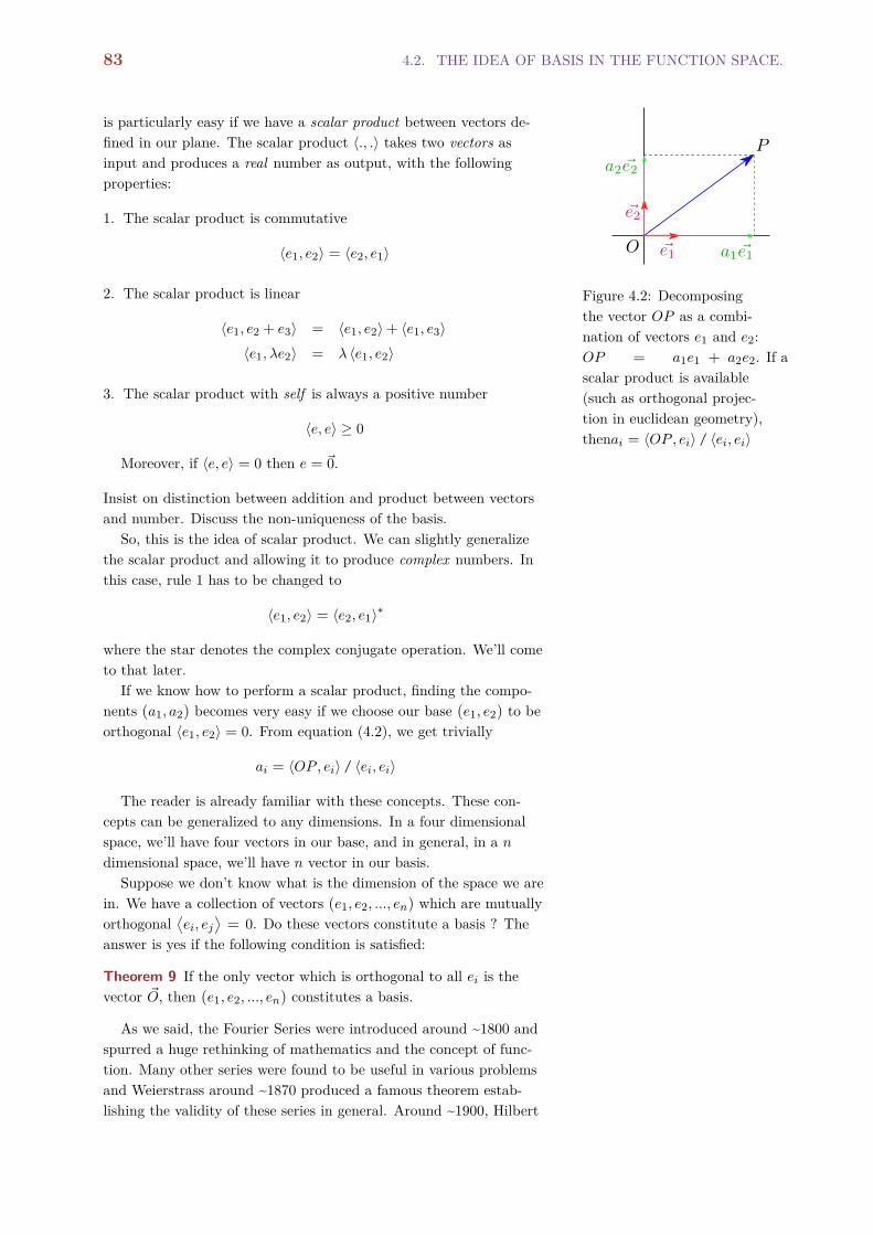
83 4.2. THE IDEA OF BASIS IN THE FUNCTION SPACE.
is particularly easy if we have a scalar product between vectors de-fined in our plane. The scalar product 〈., .〉 takes two vectors asinput and produces a real number as output, with the followingproperties:
Figure 4.2: Decomposingthe vector OP as a combi-nation of vectors e1 and e2:OP = a1e1 + a2e2. If ascalar product is available(such as orthogonal projec-tion in euclidean geometry),thenai = 〈OP , ei〉/ 〈ei, ei〉
1. The scalar product is commutative
〈e1, e2〉 = 〈e2, e1〉
2. The scalar product is linear
〈e1, e2 + e3〉 = 〈e1, e2〉+ 〈e1, e3〉〈e1,λe2〉 = λ 〈e1, e2〉
3. The scalar product with self is always a positive number
〈e, e〉 ≥ 0
Moreover, if 〈e, e〉 = 0 then e = ~0.
Insist on distinction between addition and product between vectorsand number. Discuss the non-uniqueness of the basis.
So, this is the idea of scalar product. We can slightly generalizethe scalar product and allowing it to produce complex numbers. Inthis case, rule 1 has to be changed to
〈e1, e2〉 = 〈e2, e1〉∗
where the star denotes the complex conjugate operation. We’ll cometo that later.
If we know how to perform a scalar product, finding the compo-nents (a1, a2) becomes very easy if we choose our base (e1, e2) to beorthogonal 〈e1, e2〉 = 0. From equation (4.2), we get trivially
ai = 〈OP , ei〉/ 〈ei, ei〉
The reader is already familiar with these concepts. These con-cepts can be generalized to any dimensions. In a four dimensionalspace, we’ll have four vectors in our base, and in general, in a ndimensional space, we’ll have n vector in our basis.
Suppose we don’t know what is the dimension of the space we arein. We have a collection of vectors (e1, e2, ..., en) which are mutuallyorthogonal
⟨ei, ej
⟩= 0. Do these vectors constitute a basis ? The
answer is yes if the following condition is satisfied:
Theorem 9 If the only vector which is orthogonal to all ei is thevector ~O, then (e1, e2, ..., en) constitutes a basis.
As we said, the Fourier Series were introduced around ~1800 andspurred a huge rethinking of mathematics and the concept of func-tion. Many other series were found to be useful in various problemsand Weierstrass around ~1870 produced a famous theorem estab-lishing the validity of these series in general. Around ~1900, Hilbert

CHAPTER 4. THE FOURIER SERIES. 84
made the connection between Fourier (and other series) and the con-cept of geometry we discussed above. Hilbert realized that a largeclass of functions can be considered just like points in a big spaceF 2. In these space, we can find an enumerable set of functions 2 which we now call the Hilbert space
(e1(.), e2(.), ...en(.), ...) which form the basis in this space. Any otherfunction f(.) can be written as a combination of the element of thebasis:
f(.) =∞∑n=0
aiei(.) (4.3)
The only difference with the preceding discussion is that the dimen-sion of the space is a small infinite, which we call enumerable.
Moreover, we already have a natural scalar product in the spaceof functions F [0,L] defined on the [0,L] interval
〈f(.), g(.)〉 =ˆ L
0f(x)g(x)dx (4.4)
which has all the nice properties of the scalar product we discussedabove. So once given a basis (e1(.), e2(.), ...en(.), ...), the coefficientsai of the decomposition ( 4.3) are directly given by
0.0 0.2 0.4 0.6 0.8 1.0−1.0
−0.5
0.0
0.5
1.0
cos(1. )
sin(1. )
0.0 0.2 0.4 0.6 0.8 1.0−1.0
−0.5
0.0
0.5
1.0
cos(2. )
sin(2. )
0.0 0.2 0.4 0.6 0.8 1.0
x/L
−1.0
−0.5
0.0
0.5
1.0cos(3. )
sin(3. )
Figure 4.3: The first three ele-ments of the Fourier basis forthe functions L1[0,L]
ai =1ri
ˆ L
0f(x)ei(x)dx
where the coefficient ri is simply the normalization factor
ri =
ˆ L
0e2i (x)dx
The only problem of working in infinite dimensional space is thatit can sometimes be tricky, and the series can diverge. The problemof convergence of such series, which we take for granted for reason-able functions (see definition 5 on page 82), took mathematicians agood amount of time; we don’t detail their beautiful works here.
Now, coming back to our Fourier series, we can see that the func-tions 1, cos(2πnx/L), sin(2πnx/L) constitute one basis (see figure4.3) for the space of F [0,L] which are L1. It is straightforward tocheck that these functions are orthogonal. The fact that they con-stitute indeed a complete basis is insured by the famous Weierstrasstheorem we mentioned. The component ai, bi are called the spectrumof the function or the amplitudes of its harmonics.
0.0 0.2 0.4 0.6 0.8 1.0
x
0.00
0.05
0.10
0.15
0.20
0.25
0 1 2 3 4 5 6 7 8 9 10
n
−0.15
−0.10
−0.05
0.00
0.05
0.10
0.15
0.20
an
Figure 4.4: The Cartesian rep-resentation of the functionf(x) = x(1 − x) and its spec-trum (equation 4.1). Thesetwo representations contain thesame information.
Recall that a function f(.) over [0,L] was defined as a table,where in one column we list all numbers in [0,L] and in the othercolumn their corresponding values. But knowing the coefficientsai, bi implies that we also know the function f(.). So another way ofdefining a function f(.) is to list all elements ai, bi in a table, calledthe spectrum of the function (figure 4.4). These are two differentviews of the same information about the function. The incrediblefact is that the are much less ai, bi coefficients that real numbers in[0,L]. Indeed, Cantor around ~1880 established that these numbersare not enumerable. So presenting the function by its spectrum ismuch more economical than by listing all f(x).

85 4.3. EXAMPLES OF FOURIER SERIES.
The other nicety about using the spectrum of the function is thatto give a good approximation of many functions, we can restrict thespectrum to a handful of coefficient, which makes the idea of usingFourier series even more appealing.
Finally, there is a nice relation relating´I f(x)
2dx and its spec-trum, called the Parceval relation:
1L
ˆ L
0f(x)2dx = a2
0 +12∑n=1
(a2n + b2
n) (4.5)
The fact is that very often, the above integral is related to quanti-ties such as the energy. What we see is that knowing the coefficientsai, bi, we can easily computing this integral. In many problems, thefunction f(.) is the solution of some differential equation and it ismuch easier to compute its Fourier components directly. The Parce-val relation allows us to access directly quantities such as the energydirectly from the spectrum.
4.3 Examples of Fourier series.
4.4 Sine and Cosine series.
We saw that the functions (1, sin(2kx), cos(2kx), ..., sin(2nkx), cos(2nkx), ...)constitute a basis in the space of functions over [0,L], where k =
π/L. But this is of course not the only basis and we can many dif-ferent ones. For example, the basis3 3 I don’t demonstrate it here, but
this basis is obtained for the Fourierbasis but a smart recombination.see my more advanced lectures inmathematics, on the same web site(in French).
(sin(kx), sin(2kx), ... sin(2nkx), ...)
is another orthogonal basis. This is called the Sine basis, as it con-tains only sines. Note that although we have only sines, we have“twice” as much as in Fourier basis, where we had only even harmon-ics (of the form 2nkx). So any (reasonable) function over [0,L] canbe written as
f(x) =∞∑n=1
bn sin(nkx)
where k = π/L and
bn =2L
ˆ L
0f(x) sin(nkx)dx
Note that for x = 0 and x = L, the series is exactly 0. Therefore, theSine series is well adapted to functions for which f(0) = f(L) = 0.
For example, the function x(1 − x) which we had decomposedin the Fourier basis (eq. 4.1) can also be decomposed in the “sine”basis (figure 4.5): 0.0 0.2 0.4 0.6 0.8 1.0
x
0.00
0.05
0.10
0.15
0.20
0.25
0.30
x(1− x)
S2(x)
S4(x)
Figure 4.5: Decomposition ofx(1 − x) over [0, 1] using sineseries, with only 2 and 4 har-monics.
x(1− x) = 4π3
∞∑n=1
(1− (−1)n)n3 sin(nπx/L)
Another useful basis is the Cosine basis
(1, cos(kx), cos(2kx), ... cos(nkx), ...)

CHAPTER 4. THE FOURIER SERIES. 86
and a function can be written in this basis as
f(x) = a0 +∞∑n=1
an cos(nkx)
where
a0 =1L
ˆ L
0f(x)dx
an =2L
ˆ L
0f(x) cos(nkx)dx Theorem 10 Series derivation
A cosine series can always bedifferentiated term by term. A sineseries can be differentiated term byterm only if f (0) = f (L) = 0.
The Cosine series are more “robust” than the Sine series, in thesense that we can derive the series term by term to have the deriva-tive of the function
f ′(x) = −k∞∑n=1
nan sin(nkx)
We can do this operation for the Sine series
f ′(x) = k
∞∑n=1
nbn cos(nkx)
only if f(0) = f(L) = 0. Using one or this three basis is dictated bythe problem at hand and its boundary values.
4.5 Complex Fourier series.
We saw at the beginning of this lecture that a function defined on[0,L] can be written as
f(x) = a0 +∞∑n=1
(an cos (nkx) + bn sin (nkx)) (4.6)
where k = 2π/L and
a0 =1L
ˆ L
0f(x)dx
an =2L
ˆ L
0f(x) cos (nkx) dx
bn =2L
ˆ L
0f(x) sin (nkx) dx
On the other hand, we know how ( see eqs. 3.1) to write sin and cosas a function of complex exponential:
cos(x) =(eix + e−ix
)/2 ; sin(x) =
(eix − e−ix
)/2i
and therefore, we can rearrange the terms inside the sum in relation(4.6)
an cos (nkx) + bn sin (nkx) = cneinkx + c−ne
−inkx
wherecn = (an − ibn)/2 ; c−n = (an + ibn)/2

87 4.6. THE VIBRATING STRING.
This rearranging allows for a more symmetric representation ofthe function f(x):
f(x) =∞∑
n=−∞cne
inkx
wherecn =
1L
ˆ L
0f(x) exp (−inkx) dx
4.6 The vibrating string.
Many area of physics are investigated by partial differential equa-tions (PDE): diffusion of heat, propagation of sound or electromag-netic waves, the movement of fluids, ... We are much less able tosolve PDEs than ordinary differential equations (ODE). The Fourierseries in many of these problems allows us to transform a PDE intoODEs. A fundamental example is the vibrating strings; if we knowhow to manage this problem, we can manage most of the problemscited above.
Figure 4.6: The vibrating stringat a given time t.
Consider a tensed elastic string fixed at its two end (such as apiano string), which we note 0 and L. The string itself is modeled byits height u(x, t) at position x at time t. The movement of the stringis given by the equation
ρ∂2u
∂t2− κ∂
2u
∂x2 = 0 (4.7)
where ρ is the density of the string and κ its elastic constant. Notethat ∂tu(x, t) is just the vertical speed of the string at position x, sothe first term of the above PDE is just the acceleration of the stringat position x. The other term is the force exerted by point aroundthe position x on the string. If the string is straight, there is noforce. Relation (4.7) is therefore just a generalization of the Newtonequation of movement ma = F to the case of continuum object.
In order to solve this PDE, we also need to have the initial stateof the vibrating string, namely its shape and its initial speed, and itsvalue at the boundaries:
u(x, 0) = f(x) (4.8)ut(x, 0) = g(x) (4.9)u(0, t) = u(L, t) = 0 (4.10)
where ut(x, t) = ∂u(x, t)/∂t.We don’t know how to solve PDE, but at any time, we can repre-
sent the function u(x, t) by its series. Condition (4.10) behooves usto use the Sine series
u(x, t) =∞∑n=1
bn(t) sin(nkx) (4.11)
where k = π/L. Note that as the strings changes its shape as afunction of time, the coefficients bn are themselves function of timebn = bn(t). We can derive this function as a function of x because

CHAPTER 4. THE FOURIER SERIES. 88
the boundary values are the correct one, getting a cosine series. Wecan derive this second series one more time because the cosine seriesare “robust”. So, plugging expression (4.7), we find
∞∑n=1
[bn(t) + n2ω2
0bn(t)]
sin(nkx) = 0 (4.12)
where ω20 = (κ/ρ)k2. The only way a Sine series can be 0 for all x is
that all its coefficients must be zero:
bn(t) + ω2nbn(t) = 0
where ωn = nω0. The solution of the above equation is
bn(t) = Bn sin(ωnt+ φn)
where Bn and φn are integration constant, and the solution is then
u(x, t) =∞∑n=1
Bn cos(ωnt+ φn) sin(nkx)
To find Bn and φn, we must use the initial conditions. The functionf(x) is known, let us call βn its Sine coefficients. Then the initialcondition (4.8) implies that we must have
Bn cos(φn) = βn
Let us for the sake of simplicity, have g(x) = 0. This implies thatwe must have φn = 0 and finally, the full solution is
u(x, t) =∞∑n=1
βn cos(ωnt) sin(nkx) (4.13)
We see here that the amplitude of the n−th harmonic oscillates atfrequency nω0. Let us see what that means.
Let us set L = 1 and suppose that at t = 0, u(x, 0) = x(x− 1)2,then the coefficients
Bn =4 (2 + (−1)n)
π3n3
For simplicity, we’ll also suppose that κ/ρ = 1, so k = π and ω0 = π
(figure 4.7).
4.7 Some other Orthogonal bases.
4.8 The Fourier Transform.

89 4.8. THE FOURIER TRANSFORM.
0.0 0.2 0.4 0.6 0.8 1.0
−0.10
−0.05
0.00
0.05
0.10
n=1
t=0
0.0 0.2 0.4 0.6 0.8 1.0
−0.06
−0.04
−0.02
0.00
0.02
0.04
0.06
n=2
0.0 0.2 0.4 0.6 0.8 1.0
−0.006
−0.004
−0.002
0.000
0.002
0.004
0.006
n=3
0.0 0.2 0.4 0.6 0.8 1.0
−0.006
−0.004
−0.002
0.000
0.002
0.004
0.006
n=4
0.0 0.2 0.4 0.6 0.8 1.0
−0.10
−0.05
0.00
0.05
0.10
t= τ/4
0.0 0.2 0.4 0.6 0.8 1.0
−0.06
−0.04
−0.02
0.00
0.02
0.04
0.06
0.0 0.2 0.4 0.6 0.8 1.0
−0.006
−0.004
−0.002
0.000
0.002
0.004
0.006
0.0 0.2 0.4 0.6 0.8 1.0
−0.006
−0.004
−0.002
0.000
0.002
0.004
0.006
0.0 0.2 0.4 0.6 0.8 1.0
−0.10
−0.05
0.00
0.05
0.10
t= τ/2
0.0 0.2 0.4 0.6 0.8 1.0
−0.06
−0.04
−0.02
0.00
0.02
0.04
0.06
0.0 0.2 0.4 0.6 0.8 1.0
−0.006
−0.004
−0.002
0.000
0.002
0.004
0.006
0.0 0.2 0.4 0.6 0.8 1.0
−0.006
−0.004
−0.002
0.000
0.002
0.004
0.006
0.0 0.2 0.4 0.6 0.8 1.0
−0.10
−0.05
0.00
0.05
0.10
t=3τ/4
0.0 0.2 0.4 0.6 0.8 1.0
−0.06
−0.04
−0.02
0.00
0.02
0.04
0.06
0.0 0.2 0.4 0.6 0.8 1.0
−0.006
−0.004
−0.002
0.000
0.002
0.004
0.006
0.0 0.2 0.4 0.6 0.8 1.0
−0.006
−0.004
−0.002
0.000
0.002
0.004
0.006
0.0 0.2 0.4 0.6 0.8 1.0
−0.10
−0.05
0.00
0.05
0.10
t= τ
0.0 0.2 0.4 0.6 0.8 1.0
−0.06
−0.04
−0.02
0.00
0.02
0.04
0.06
0.0 0.2 0.4 0.6 0.8 1.0
−0.006
−0.004
−0.002
0.000
0.002
0.004
0.006
0.0 0.2 0.4 0.6 0.8 1.0
−0.006
−0.004
−0.002
0.000
0.002
0.004
0.006
0.0 0.5 1.0
x
−0.15
−0.10
−0.05
0.00
0.05
0.10
0.15
u
0.0 0.5 1.0
x
−0.15
−0.10
−0.05
0.00
0.05
0.10
0.15
0.0 0.5 1.0
x
−0.15
−0.10
−0.05
0.00
0.05
0.10
0.15
0.0 0.5 1.0
x
−0.15
−0.10
−0.05
0.00
0.05
0.10
0.15
0.0 0.5 1.0
x
−0.15
−0.10
−0.05
0.00
0.05
0.10
0.15
Figure 4.7: The shape of vi-brating string (lower row, redcurves) at different times whereτ = π/ω0 . The blue curvesare the first four harmonics forharmonics bn(t) sin(nπx) forthe same times. Note the scaleof the vertical axis for eachharmonics.


Chapter 5
Linear Algebra.
Contents
5.1 Why linear algebra is such a fundamental topic. 92
5.2 Linear systems. 92
5.3 Vectors. 93
5.3.1 Linear Independence. 95
5.3.2 The concept of basis. 95
5.4 Linear Application. 96
5.5 Solving a linear system. 96
5.5.1 The Determinant. 96
5.5.2 Determinant as an antisymmetric application. 97
5.5.3 The Kernel. 97
5.6 Numerical methods. 97
5.7 Eigenbasis and matrix diagonalization. 97
5.8 Tensors. 97

CHAPTER 5. LINEAR ALGEBRA. 92
5.1 Why linear algebra is such a fundamentaltopic.
Consider the following problems :
1. Solve the two equations, two unknown system x+ y = 1 ; 2x−3y = 0
2. Find the plane vector that under a π/6 rotation around the pointO transforms into a known vector.
3. Solve the differential equation y′′ + 4y′ + 2y = sin(x/6)
4. Solve the partial differential equation ∂tu−D∂xxu = Q(x, t)
These are problems arising in algebra, in geometry and in analysis.These, and many other problems arising in physics and mathematics,are just the same thing. If you know how to solve the first question,you should know how to solve the others listed above.
OK, I said you should. This is not that obvious at first, and infact, the similarity between these subjects become understood reallyat the beginning of the XX-th century, mostly through the work ofa mathematician called Hilbert. Physicist grabbed the power be-hind this unification in the 1920’s, with the advance of the quantummechanics (you needed a PhD at these times to have heard aboutmatrices). However, this is such a powerful understanding1 that it is 1 This is our version of getting out
of the cave and look directly at theLight. And contrary to the guywho invented this tale, nobody gotharmed by learning this tool and it isnot the sole domain of some electedpeople.
taught nowadays at the very end of high school and beginning of theuniversity, to hard science students.
So, what we are going to do is to learn how to efficiently solvesimple equation of type 1, and then use these results for the variousother types of problems we’ll encounter.
5.2 Linear systems.
Let us do some generalization by considering a linear2 system of 2 The word linear will be definedshortly.n equations and n unknowns. We will designate the unknown by
x1, ...,xn. The known parameters of these equations would be calledaji (we have n2 of them). The element of the right hand side will benoted b1, ..., bn. The n× n system can now be written very generallyas
a11x1 + a2
1x2 + ... + an1x1 = b1
a12x1 + a2
2x2 + ... + an2x1 = b2...
......
a1nx1 + a2
nx2 + ... + annx1 = bn
For a large system, this is a little long to write. We can push a littleour symbols : collect all parameters into an object A = aji, all theunknowns into an object x = xi and all right hand side into anobject b = bi. the collection x and b will be called vector here.

93 5.3. VECTORS.
The collection A will be called a matrix. We can now symbolicallywrite the above system as
Ax = b (5.1)
which present some similarity to the way we write a basic equationsuch as ax = b ( 3x = 2) which we will call a scalar equation. Togo beyond the analogies, we have to define what is a multiplicationbetween a matrix and a vector. But before doing that, let us comeback at what is so fundamental in a simple multiplication.
Consider the basic scalar equation ax = b. We’ve learned how tosolve it when we were kids and we are so used to it that we forgethow fascinating it is. It has two very important properties:
1. Suppose that given a and b, we have solved the equation ax = b
and called the solution x0. What is the solution of the equationax = 2b ? Obviously, the solution this time is x1 = 2x0. Inother terms, if we multiply the right hand side by a factor λ, thesolution is also multiplied by λ.
2. Suppose now that we have solved ax = b1 (solution called x1) andthe equation ax = b2 (solution called x2). What is the solution ofax = b1 + b2 ? Obviously, the solution is x1 + x2.
The above two properties characterize what is called the linearity ofthe system. If we look at the four problems listed at the beginning ofthis chapter, they all share this properties.
Now, let us more precisely come to the system (5.1). Considermultiplying all elements of b by the same factor λ. Obviously, allelements of the solution x will also be multiplied by λ (compared tooriginal solution). The same argument can be repeated for additionof b1 + b2. So the system of n× n equation has the properties oflinearity, and this is why we call it a linear system.
If we are interested to just solve equation (5.1), we can use thepivot or Gauss-Bonnet method, which will involve some n2 operationof addition and multiplication. We’ll come to that later. But we willmiss important concepts. For example, can any linear system besolved ? Consider for example the linear system
x+ y = 1 ; 2x+ 2y = 2
Obviously, there is no unique solution to this system. For example,x = 0.25 and y = 0.75 is a solution ; so is x = y = 0.5. On the otherhand, the linear system
x+ y = 1 ; 2x+ 2y = 3
has no solution. Existence and uniqueness are at the heart of linearsystems and we need a broader view of these system in order to beable to give very general arguments on them.
5.3 Vectors.
Let us forget about numbers, and define a collection of objects vwe’ll call vectors. We will call the ensemble of all these objects a

CHAPTER 5. LINEAR ALGEBRA. 94
vectorial space E . You can picture a vector for example as a finiteline with an arrow on it, like the geometric vectors of a plane.
For each ensemble, we know how to do two basic operations withvectors : we can add two vectors v1 and v2, which results in anothervector3. We can multiply a vector v by a number λ, which again 3 Addition has to be commutative to
be called additionresults in another vector.
Example 1: The best example for an object which has the vectorproperty is an n−tuple of numbers v = (x1, ...,xn) : we putn−numbers into an ordered bag we call a tuple. The addition oftwo vectors is obtained by adding the respective elements:
(x1, ...,xn) + (y1, ..., yn) = (x1 + y1, ...,xn + yn)
multiplying by a vector is
λ(x1, ...,xn) = (λx1, ...,λxn)
Example 2: The next best example are geometric vectors in theplane (or in a d−dimensional space), were we have learned thebasic rules of addition and multiplication (figure 5.1).
Figure 5.1: geometric vectors:addition and multiplication bya number.
Let us say, a little in advance, that geometric vectors are alson−tuples.
Example 3: Consider polynomials of the forms
P (x) = a0 + a1x+ a2x2 + ...anxn
Of course, we know how to add polynomials and multiply them bya number, so each polynomial can be considered a vector. This isnot a very new kind of vector, as each polynomial can be writtenas a n−tuple (a0, a1, ..., an) and the power of x are just used asa short hand for place holder. So in fact, we are back to the firstexample, although here we used a special kind of functions.
Example 4: Consider general real functions f(x) (f : R → R).Again, we know how to add functions and multiply them by anumber. So each function is a vector by itself. Are functions thesame thing as n−tuples ? The question seems rather strange andthe analogy is not clear at all.
0.0 0.5 1.0 1.5 2.0 2.5 3.0 3.5 4.0
x
−2
−1
0
1
2
3
sin(x) 2sin(x)
sin(x) +exp(x/4)
exp(x/4)
Figure 5.2: grah of two func-tions, their addition and multi-plication by a number
But the full power of linear algebra was unleashed when peoplerealized that indeed, there is a close connection between func-tions and n−tuples and useful functions (all the ones we use inreal world) are indeed n−tuples. We’ll come to that later in thischapter. The first person who saw the connection was Fourieraround 1800 but the full picture was given by Hilbert by the endof XIX-th century.
Oh, I forgot, for a collection of vectors to be called a vectorial space,we need to have a unique element, called the ~0 vector, such thatv+~0 = v.

95 5.3. VECTORS.
5.3.1 Linear Independence.
Consider n non zero vectors. If we can write one (say v1 ) as thecombination of the others
v1 = a2v2 + a3v3 + ... + anvn (5.2)
(where ai are numbers) we say that these vectors are linearly depen-dent. Another way of saying that these vectors are linearly depen-dent is to state that there are numbers ai, not all of them zero, suchas ∑
i
aivi = ~0 (5.3)
As an exercice, you can demonstrate that statements (5.2,5.3) areequivalent.
On the other hand, we say that n−vectors are linearly indepen-dent if we cannot write one as the combination of others. We wouldsay that for these vectors, statement (5.3) implies that all ai = 0.
Insist on the distinction between numbers and vectors.
5.3.2 The concept of basis.
Consider a vectorial space E , where we have found n vectors e1, ..., ensuch that
1. ei are independent.
2. Any vector of E can be written as a combination of ei. Inmathematical terms,
∀v ∈ E , ∃ai such that v =∑i
aiei (5.4)
If we have such vectors ei, we say that they constitute a basis forE . The n−tuples (a1, ..., an) of relation (5.4) for a vector is calledthe decomposition of this vector on the ei basis.
Exercise: demonstrate that a decomposition is unique.
Example 1: the tuples (1, 0) and (0, 1) are a basis for the real twotuples. So are the tuples (1, 1) and (−1, 1) (Demonstrate).
Example 2: any two non-collinear vectors of the plane are a basis forthe plane.
Example 3: For functions defined on a finite interval [0,L] andwhose [...], the functions cos(nπx/L),n = 0, 1, ... constitute abasis.
Well, example 3 needs some developments before getting used to. Ididn’t say what is the condition inside the [...], we’ll see that later.Let us just say that the above basis is called a Fourier series. Theimportant thing to understand is that having a basis is the bridgebetween tuples and vectors.

CHAPTER 5. LINEAR ALGEBRA. 96
5.4 Linear Application.
Consider a special class of functions which takes a vector as an inputand produce a vector as an output
u = f(v)
5.5 Solving a linear system.
5.5.1 The Determinant.
Before going to the full solution of the system A |x〉 = |b〉, we havefirst to ask two questions : Does a solution exists ? Is the solutionunique ? The answer to these questions has nothing to do with theright hand side |b〉, and everything to do with the structure of thematrix A. So let us for the moment focus on the simpler equation
A |x〉 = |0〉
To make things more concrete, consider the 2× 2 system
ax+ by = 0cx+ dy = 0
where x, y are the unknown and a, b, c, d the known parameters. Wecan compute the value of y from both equation y = −a/b = −c/d.Obviously, in order not to run into a contradiction, we must havea/b = c/d or in other words,
ad− bc = 0 (5.5)
The number ad− bc for a 2× 2 matrix is called its determinant, andnoted |A|.
The meaning of the determinant however doesn’t really depend onthe numbers of the matrix. As we said, a matrix is just one represen-tation of a linear application. Given a basis |ei〉, we can representthe linear application A by the collection of vectors |Aei〉. The de-terminant of the application A is a number that determines if thesevectors |Aei〉 are independent! In fact, if the determinant is exactlyzero, these vectors are linearly dependent.
Figure 5.3: The surface definedby two vectors can be used todetermine if they are indepen-dent.
How can we construct a linear dependence measurement whichis compatible with the simple criteria (5.3) ? Let us think a littlegeometrically. In a plane, if two vectors are collinear, then they aredependent. On the other hand, if they are collinear, the parallelo-gram surface they define is exactly zero.
Figure 5.4: Half-Surface cov-ered by two vectors
Suppose now that in the plane, we have two independent vectors|e1〉 and |e2〉 and we define their surface to be one unit. What is thesurface covered by the vectors |u1〉 = (a, c)T and |u1〉 = (b, d)T
? From figure ..., we see that the surface of the triangle covered bythese two vectors can be computed as follow: from the rectangle ofsurface ad, we have to subtract the surface of the three trianglesof surfaces ac/2, bd/2 and (a − b)(d − c)/2. The surface of theparallelogram is twice the surface of the rectangle, so its surface is
∆ = ad− bc

97 5.6. NUMERICAL METHODS.
5.5.2 Determinant as an antisymmetric application.
5.5.3 The Kernel.
5.6 Numerical methods.
5.7 Eigenbasis and matrix diagonalization.
5.8 Tensors.
Generalization of linear application (make the analogy with functionsof multiple variables). Outline of the elasticity (and EM ?).


Part II
Physics


Chapter 6
Mechanics.
Contents
6.1 Fundamental concepts. 102
6.1.1 Time, position, speed. 102
6.1.2 Force. 103
6.1.3 Dimensions and units. 105
6.2 The fundamental law of mechanics. 105
6.2.1 Harmonic Oscillator. 109
6.2.2 Forced harmonic oscillator. 110
6.2.3 Centripetal and Coriolis Forces. 112
6.3 Exercises: Movement. 115
6.4 Kinetic energy, work, power. 118
6.4.1 Power. 119
6.5 Potential and total energy. 119
6.6 Exercises : Energy 122
6.7 Equilibrium. 125
6.7.1 Basic concepts. 125
6.7.2 Forgetting the forces of reactions. 126
6.7.3 Torque and solid objects. 126
6.8 Exercises: Equilibrium. 129
6.9 The Lagrangian formulation. 131
6.9.1 Introduction. 131
6.9.2 Why Lagrangian mechanics ? 132
6.9.3 The Euler-Lagrange equation. 133
6.9.4 Planetary movement. 135
6.9.5 Mechanics of solid objects. 136
6.10 Exercises: Lagrangian. 137
6.11 Advanced topics: Relativity. 138
6.12 Application: the principle of an atomic force microscope. 139

CHAPTER 6. MECHANICS. 102
6.1 Fundamental concepts.
6.1.1 Time, position, speed.
A particle in space can be characterized by its position x and thetime t at which we make the observation. So we need to use fournumbers to know where and when the particle is. It took some timesfor scientists to realize that this four numbers are not really differ-ent and all the law of physics can be formulated elegantly in a 4dimensional space. Originally however, humans distinguished thetime from space and the laws of mechanics were formulated in thisframework. We will abide by this rule in this lectures.
Definition 6 the speed v, acceler-ation a and the momentum p aredefine as
v =dxdt
p = mv
a =dvdt
The speed of a particle is the rate at which it changes its position:
v =dxdt
(6.1)
If we know the position of a particle at all time in the interval[t1, t2], we can determine its speed by a simple derivation. On theother hand, if we know the speed of a particle1 during the interval 1 Imagine that you record continu-
ously the value of your speedometer.[t1, t2], we can recover its position at any time:
x(t)− x(t1) =ˆ t
t1
v(τ )dτ
The momentum of a particle is the product of its mass by itsspeed
p = mv
The acceleration is the rate of change of the speed
a =dvdt
by the same token, if you know your acceleration at any time in[t1, t2], you can determine your speed
v(t)− v(t1) =ˆ t
t1
a(τ )dτ
This is indeed how the inertial navigation works: small masses,coupled to springs are used in a device to monitor the acceleration atany time, which is numerically integrated to determine the speed and(by one more integration) the position at any time.
§ 6.1 rotation.An object rotates at constant angular frequency ω around the origin at
distance r. Compute its speed, acceleration, and the relation between them.
Solution. The position of the object is given by x = r cosωt ; y = r sinωt.Therefore, deriving twice, we have
Figure 6.1: rotation at constantangular frequency.
vx = −rω sinωt ; vy = rω cosωtax = −rω2 cosωt ; ay = −rω2 sinωt
The amplitude of these quantities is therefore
v = rω ; a = rω2

103 6.1. FUNDAMENTAL CONCEPTS.
and if we express one as the function of the other, we have
a =v2
r
The reader should check that these expressions are dimensionally correct.Note that the speed vector is tangent to the circle, while the accelerationpoints toward the origin. Discuss these remarks.
6.1.2 Force.
Objects change their speed upon the action of a force F, which ismeasured in unit of Newton (N). A 1kg mass at the surface of earthis submitted to a gravitational force of F = 9.8N.
Figure 6.2: Objects changetheir vectorial speed unpon theaction of a force.
The concept of force is less precisely defined than that of theother (geometrical) variables. Even if we don’t (yet) give a moreprecise definition of the force, we have various kind of instrumentswhich can precisely measure it2. We can for example use a spring
2 There is a circularity in force defi-nition. Force is defined as the agentthat changes speed. However, inorder to measure it, we use the rateof speed change (or various measurerelated to that). There is nothing tobe ashamed of. The ensemble is ex-tremely self coherent and allows us tomake extremely precise predictions.
and act with a force on it ; the deformation of the spring can beused to measure the force. Note that in this case, the force mea-surement is reduced to a position measurement, which we know howto do. Indeed, all humans measurements are reduced to time andposition measurements, through some calibration.
There are various kind of forces in our every day life. Let us visitsome important ones.
Gravitational force. At the surface of the earth, a constant force isexerted on all massive bodies which is directed toward the centerof the earth. The direction of the earth’s center, i.e. the verticaldirection, is indicated by a plumb line. Let uy be the upwarddirection, then
F g = −mguy (6.2)
where g = 9.8 ≈ 10m/s2 is called the gravity acceleration.In fact, this is an approximation of a more fundamental expres-sion. The gravitational attraction between two spherical bodies ofmass m and M at distance r of each other is (fog Figure 6.3: The Gravitational
force exerted by a sphere ofmass M (such as the sun) ona sphere of mass m (such asearth) is inversely proportionalto the square of their distance(eq. 6.3).
FG = m
(GM
r2
)ur (6.3)
where G = 6.7× 10⁻¹¹SI and ur is the unit vector pointing to-ward the other mass. Now, the earth mass M = 6.0× 1024kg andearth radius is r0 = 6.4× 10⁶m. putting this numbers together, wefind that at the earth surface
g = GM/r20 = 9.8m.s−2
but why the force should be constant ? Consider being at a heighth from earth surface, then the force intensity is, to first order in h
FG = mGM
(r0 + h)2 = mGM
r20
(1− 2 h
r0
)the corrective term 2h/r0 is negligible for h smaller than fewthousand of meters, the altitude of our highest mountains. So we

CHAPTER 6. MECHANICS. 104
can safely approximate the gravitational force to be constant inthese ranges.
Coulomb forces. this is the force exerted between two charges andhas the same shape as the gravitational force
FC = −Kq1q2r2 ur (6.4)
where K = 9× 10⁹SI and qi are the charges.Compare now the gravitational and Coulomb forces between anelectron and a proton at 1nm distance. The charge of an electronand a proton is |q| = 1.6× 10⁻¹⁹C, the mass of a proton is around10−27kg and an electron around 10−30kg. The Coulomb forcewould be around 10−10N, while the gravitational force wouldbe around 10−50N ! by all means, at the molecular level, we canforget about gravitation.
Solid Friction. An object sliding on a surface is subject to a solidfriction force. If R is the amplitude of the force pushing the objecttoward the surface (force perpendicular to the surface), then partof this force is converted into a force F s parallel to the surfaceand opposing the movement (fig. 6.4). The amplitude of these twoforces are proportional : Figure 6.4: The solid friction
force F s opposes the move-ment. Its amplitude is pro-portional to the perpendicularforce pushing the object againstthe surface.
Fs = µR (6.5)
This is due to the fact that the amplitude of molecular forcesbetween the two surfaces depend on R. The coefficient µ can beas high as 0.5 between two rough surfaces or close to 0 when thesurfaces are well lubricated.
Viscous drag. This force appears at low speed when an object ismoving in a liquid or gas such as water or air. This force alsoopposes the movement, but its amplitude is proportional to thespeed of the object :
Fv = −ρv (6.6)
where ρ is a coefficient which depends on the viscosity of theliquid and the shape of the object. For a sphere of radius a forexample, ρ = 6πηa, where η is the viscosity of the liquid (ηwater =10−3Pa.s). Most of the friction on a bike or a car comes fromviscous drag and not from solid friction with the road (which isclose to zero when the wheels are rotating).
Figure 6.5: The restoring forceof a spring.
Restoring forces. This kind of force appears when an elastic object isdeformed : the force acts in the direction that restores the originalequilibrium and its amplitude is proportional to the deformation.The most visual example is the spring (fig 6.5. The restoring forceis
F = −kx (6.7)
where x is the deviation from the equilibrium position and k aconstant, called the spring constant, measure in N/m (Newton

105 6.2. THE FUNDAMENTAL LAW OF MECHANICS.
per meter). The spring constant used in various devices variestypically from 10−3 N/m to 108N/m. In fact, this large rangemakes “springs” the best choice of measuring forces in manysituations.
Figure 6.6: In an opticaltweezer, a laser light is focusedinto a beam that is around 1µmin waist at its minimum. Thecenter O of the focused beamacts as an attractor for objectssuch as bacteria ; the amplitudeof the force is spring-like andproportional to the distance ofthe object from the center O.
Many devices can be built to present a spring-like force. At themicron scale for example, we can use light to make an opticaltweezer, by focusing a laser beam with a high numerical apertureobjective. Objects such as bacteria are attracted to the center ofthe focused light by such a force.
6.1.3 Dimensions and units.
Quantities in physics have units. The dimensionality of a quantitydepends on the units in which they are measured. There are fewfundamental quantities: length L, time T , mass M , charge Q. In SIsystem, we use meter (m), second (s), kilogram (kg) and Coulomb3
3 The most recent version of SI sys-tem uses Ampere as the fundamentalunit for current and charge off 1Cis defined as 1 A.S (ampere second,the amount of charge transferred in 1second by a 1 amp current)
(C) as standard units. All other quantities can be expressed in termsof combination of the above one. The speed v = dx/dt for exampleis a length divided by a time. We express that by noting
[v] = L/T
When writing an equation, all terms that add or are equal shouldhave the same dimensionality. Consider for example the equation(which we will encounter later)
md2x
dt2+ ρ
dx
dt+ kx = mg
where x is the position and t the time. The dimensionalities of theterms can be written as
MLT−2 + [ρ]LT−1 + [k]L2 =M [g]
We see here that, as M [g] = MLT−2, we must have [g] = LT−2; inother terms, g is an acceleration. The same argument indicates that
[k/m] = T−2
this has the unit of the inverse a square time. We often note k/m =
ω2, where [ω] = T−1 is a frequency, which we will see is the properfrequency of the above oscillator.
Functions can only be applied to numbers. We can computeexp(2), but we cannot compute exp(2apples)! So, if an expressionappears inside a function, it has to be a number. For example, if wehave sin(ωt) where t is a time, we must have [ω] = T−1.
When writing equations, we must always check for dimensionalhomogeneity (2 apples can never be equal to 3 oranges). Very often,some terms computed from equations will appear obviously wrongbecause of this analysis, indicating an error in the computation.
6.2 The fundamental law of mechanics.
The fundamental law of mechanics, as originally formulated by New-ton around 1680 relates all the above variable4: the rate of change in 4 This law is valid at speeds small
compared to the speed of light.

CHAPTER 6. MECHANICS. 106
momentum equals the force.
dpdt
= F (6.8)
if you know the force, you can determine how the particle is going tochange its (vectorial) speed. On the other hand, if you measure youracceleration, you know which force has acted upon you.
One of the most practical application of the fundamental law (6.8)is to determine the trajectories of object submitted to a given force.It happens very often that we know what the force is, and we needto compute its consequences on the movement of a mass submittedto this force.
Usual objects have a physical extensions. An average car for ex-ample is around 4m in length, 1.8m in height and the same in width.We would need 6 numbers to characterize a car : three numbers forits position and three numbers for its orientation. For the moment,we will suppose that objects are without extension and giving theirposition is enough. This constraint will be relaxed later when we’llstudy solid mechanics.
Let us see the application of relation (6.8) through few examples.
Example 6.1 No force.Let us suppose first that we are in a one dimensional world
where the position of the object is given by x(t). Equation (6.8)when F = 0 reads
mdv
dt= 0
and therefore
0.0 0.2 0.4 0.6 0.8 1.0
t0.4
0.6
0.8
1.0
1.2
1.4
1.6
v(t)
x(t)
Figure 6.7: v(t) and x(t) un-der “no force” condition. Notethat x and v have different di-mensionality and should be,in principle, be drawn in twodifferent graphs.
v(t) = v0
where v0 is a constant. If at time t = 0, the speed is v0, then atall further times, the speed will remain at this value. We say thatthe momentum p (or the speed v) is conserved (figure 6.7). By thesame token, we have
x(t) = x0 + v0t
As trivial as it may seem, this was the fundamental paradigmshift which happened by the work of Galileo and formally, byNewton. The Aristotelian physics stipulated that to have move-ment, we need to exert force. The new physics stipulated thatforce only changes the speed, but we can have non-zero movementin the absence of force.
In three spatial dimension, we have a natural extension of thislaw
v(t) = v0 ; x(t) = x0 + v0t
Example 6.2 Constant force.Consider know the case of constant force F = F0. Such a force
arouses for example in free fall under the force of gravity
F0 = −mg

107 6.2. THE FUNDAMENTAL LAW OF MECHANICS.
where m is the mass of the object and g a constant associated tothe terrestrial attraction (g = 9.8m2/s ). Let us denote the heightof the object by y(t) and v(t) = y(t). Then
mv(t) = −mg
and therefore
v(t) = −gt+ v0 ; y(t) = y0 + v0t− (1/2)gt2
We observe that the position and speed of the object does not de-pend on its mass. The demonstration was made by Galileo bydropping objects from a tower.
Consider now a two dimensional world where x(t), y(t) denotethe horizontal and vertical position of the object, and where thereis no force in the horizontal projection: F = (Fx,Fy), Fx = 0 andFy = −mg. Then obviously,
0.0 0.2 0.4 0.6 0.8 1.0
t−2.0
−1.5
−1.0
−0.5
0.0
0.5
1.0
x(t)
y(t)
0.0 0.2 0.4 0.6 0.8 1.0
x−1.0
−0.5
0.0
0.5
1.0
y
Figure 6.8: Movement underthe constant force of free fall
x(t) = x0 + v0,xt (6.9)y(t) = y0 + v0,yt− (1/2)gt2 (6.10)
where v0 = (v0,x, v0,y) is the initial vectorial speed of the object.Usually, we choose the origin of the coordinates such that x0 =
y0 = 0. If we throw the objects with the initial positive speed v0,y,at time t∗ = 2v0,y/g the object is back to the surface. We canalso eliminate t in relation (6.9-6.10) and write y as a function ofx:
y(x) =v0,yv0,x
x− g
2v20,xx2
The function y(x) is called the trajectory of the object. If wetake successive photograph of th e object and superpose them, wewould observe this function.
Example 6.3 Slide.
Figure 6.9: Slide
Consider an object on a slide, where the solid friction coef-ficient is µ. The object is subjected to two forces : the gravityF g and the solid friction F s. There is also a reaction force ofthe slide on the object which is perpendicular to the slide. As weare interested in the movement along the slide, we choose the xaxis along it. The mentioned reaction force is perpendicular tothis axis and therefore has no influence on the movement alongthis axis. This is why the reaction force is not represented on thefigure5. 5 For a deeper discussion of reaction
forces, see section 6.7.The amplitude of the gravity force Fg = mg. This force can bewritten as the sum of two forces parallel and perpendicular to theslide:
F g = F⊥g +F‖g
We know that F⊥g = mg cos θ and therefore Fs = µmg cos θ. Onthe other hand, F ‖g = −mg sin θ. For the movement along theslide, we thus have
a = −g(sin θ− µ cos θ)

CHAPTER 6. MECHANICS. 108
We see here that this is similar to the free fall we have in theprevious example. But, even when µ = 0 (no friction), the acceler-ation is smaller than g by a factor sin θ. Obviously, if θ = 0, thereis no sliding. On the other hand, we see that when µ > 0, there isan angle θ∗ = arctan(µ) for which the acceleration vanishes. Nomovement is possible6 when θ < θ∗. This is why we can walk on 6 The discussion is slightly more com-
plex because the amplitude of thefriction force is higher when there isno movement : µstop > µmovmemnt.
inclined plane without falling.
Example 6.4 Movement in a magnetic field.When charges move in a magnetic field B, a force proportional
to their speed is exerted upon them. We use traditional notationfor coordinates (x, y, z) and denote by (vx, vy, vz) the speed inthese directions. We suppose a constant magnetic field in thedirection of the z axis B = Buz. Then for a charge q, the force is
F = (qBvy,−qBvx, 0)
This expression is called the Laplace force and in vectorial nota-tion is written as F = q v∧B. Note that this is the first examplewe see where the force is a function of the characteristic of theobject (here the speed). The fundamental law (6.8) is therefore
dvxdt
= ωvy (6.11)
dvydt
= −ωvx (6.12)
dvzdt
= 0 (6.13)
where ω = qB/m. Note that ω has the dimension of an inverseof time (a frequency). The last equation is a movement under notforce and we have vz = vz,0. The two first equation constitutea a system of two first order equations. There are many ways ofsolving these equations.
For example, if we derive the first equation (in respect to time)and use the second equation for the value of vy, (and do the samefor the other equation) we have
vx + ω2vx = 0vy + ω2vy = 0
A better, simpler way would be to introduce the complex speed
V (t) = vx(t) + ivy(t)
then obviouslyd
dtV = −iωV
whose solution is simply
x
−1.0
−0.5
0.0
0.5
1.0
y
−1.0
−0.5
0.0
0.5
1.0
z
0
5
10
15
20
25
Figure 6.10: Trajectory un-der constant magnetic force.The magnetic field is in the zdirection.
V (t) = V0e−iωt (6.14)
We observe that∣∣V (t)
∣∣ = ∣∣V0∣∣: the amplitude of the speed remain
constant, only its direction rotates at frequency ω. This is the

109 6.2. THE FUNDAMENTAL LAW OF MECHANICS.
main characteristic of magnetic force ; as we will see below, wesay that this force does not work.
Let us choose the orientation of our axes in such a way thatvx,0 = v, vy,0 = 0 (we choose the x axis to be parallel to theinitial speed). Then the complete solution is
vx(t) = v cos(ωt) ; vy(t) = −ν sin(ωt) ; vz = vz,0
and the position is obtained by integrating these equations oncemore. Note that the trajectory of the charge is a spiral (figure6.10).
Many phenomena we observe around us are just oscillations: soundwaves, earthquakes, radio reception, small movements of bridges andbuildings, ... The lord of all these rings is the harmonic oscillator,used to capture the essence of all these phenomena.
6.2.1 Harmonic Oscillator.
Consider a small ball attached to the end of a spring. We take therest position of the spring as the origin. If now we move the ball to anew position and let it free, the ball will perform oscillation.
Figure 6.11: A ball attached toa spring. The origin is taken asthe rest position of the spring.
The amount of force exerted by the spring on the ball at positionx is
F = −kx
where k is called the spring constant. Here, the force depends on theposition of the object. The fundamental law reads
md2x
dt2+ kx = 0
which is a second order ODE which we know how to solve (Chap-ter 2, section 2.4). Noting ω2 = k/m, which is called the naturalfrequency of the oscillator, the solution is
x(t) = A cos(ωt) +B sin(ωt)
If at time t = 0, x(0) = x0 and v(0) = v0, the solution is
x = x0 cos(ωt)
and the ball oscillates indefinitely.We know however that the real movement is damped. This is
because of friction forces due to air or liquid molecules. The frictionforce is of the form
Ffr = −ρv
which means that it always opposes the movement. Writing 2ν =
ρ/m, the complete equation of the movement is0 5 10 15 20 25 30
−1.0
−0.5
0.0
0.5
1.0
ν=0
ν=0. 1
ν=0. 5
ν=0. 95
Figure 6.12: oscillation underharmonic and friction forces.ω = 1, x0 = 1, v0 = 0.
d2x
dt2+ 2ν dx
dt+ ω2x = 0
Noting Ω2 = ω2 − ν2, we know that the solution of the aboveequation for the same initial condition is
x = x0e−νt cos(Ωt)

CHAPTER 6. MECHANICS. 110
which is a damped oscillation. Of course, if Ω2 < 0, the solution hasno oscillation
x(t) = Ae
(−ν+√ν2−ω2
)t +Be
(−ν−√ν2−ω2
)t
and is totally damped.
6.2.2 Forced harmonic oscillator.
Now, let us go one step further and consider a ball attached to thespring and submitted to friction and another external force F (t): abridge under the wind, an electrical RLC circuit receiving a signal,electron in an atom receiving an electromagnetic field... the equationof the movement is
md2x
dt2+ ρ
dx
dt+ kx = F (t) (6.15)
As usual, we callω0 =
√k/m
the natural frequency of the oscillator and note ν = ρ/m the damp-ing coefficient.
If for example F (t) = F0 = Cte, the ball, after few oscillations,will move to a new position x = F0/k and stay at this value.
The most interesting case however is when the forcing is itself aperiodic signal at frequency F = F0 cos(ωf t), where the equation ofmovement is
d2x
dt2+ ν
dx
dt+ ω2
0x = a cos(ωf t) (6.16)
where a = F0/m. After a temporary time, the memory of the initialcondition is lost (because of the damping) and the ball begins tooscillate at the forcing frequency ωf (and not at its own naturalfrequency ω0). To see this, let us try the tentative solution 0 5 10 15 20 25 30
t
−2.0
−1.5
−1.0
−0.5
0.0
0.5
1.0
1.5
2.0x(t)
f(t)
2
1. 5
1. 0
0. 25
Figure 6.13: Periodically forcedharmonic oscillator. x(t) forvarious values of ω0/ωf . In thisexample, a = 1, ν = 0.5 andωf = 1.
x = A cos(ωf t) +B sin(ωf t) (6.17)
and plug it into equation (6.17). Can we find the amplitudes A andB ? Deriving twice and grouping terms in cosine and in sine, wehave (
−Aω2f +Bνωf +Aω2
0
)cos(ωf t) +(
−Bω2f −Aνωf +Bω2
0
)sin(ωf t) = a cos(ωf t)
And if we want this relation to be valid, we must have(ω2
0 − ω2f
)A+ νωfB = a
−νωfA+(ω2
0 − ω2f
)B = 0
This is an linear algebraic system of two equations and two un-known, which is readily solved. Let us set
δ =(ω2
0 − ω2f
)

111 6.2. THE FUNDAMENTAL LAW OF MECHANICS.
which is called the detuning. The solution is
A =δ
δ2 + (νωf )2 a
B =(νωf )
δ2 + (νωf )2 a
So relation (6.17) is indeed the solution of equation (6.16). Figure6.13 shows the function x(t) for various ratio of ω0/ωf . 10-1 100 101
ωf/ω0
10-2
10-1
100
101
102
R/a
ν=1
ν=0. 5
ν=0. 25
ν=0. 1
ν=0. 02
Figure 6.14: The amplificationR/a as a function of forcingfrequency ωf/ω0 for variousvalues of damping ν. In thisexample, ω0 = 1.
Let us set
R2 = A2 +B2 =a2
δ2 + (νωf )2
tan(θ) =B
A=
(νωf )
δ
Then relation (6.17) can be written
x(t) = R cos(ωf t− θ)
R is the oscillation amplitude and θ the phase shift.We see here that both the amplitude R and the phase shift θ
are functions of ωf . Figure 6.14 shows the vibration amplitude asa function of the forcing frequency. The maximum amplitude isreached when the forcing frequency equals the natural frequency(δ = 0). This is called resonance and in this case
Rres =a
(νωf )
and if the damping is small, the resonance amplitude can be ex-tremely high.
Note that when ωf → 0, R/a ≈ 1/ω20 ; on the other hand, when
ωf ω0,R/a ≈ 1/ω2f .
The high value of R at resonance (for small damping) is used forsignal amplification. When you are trying to detect a signal with aninstrument (being mechanical, electrical, ...) you devise an instru-ment which in effect is a harmonic oscillator, where you can changeits natural frequency by some control. For example, you can changeits spring constant. The device is submitted to the signal whichplays the role of the external force. To detect efficiently the signal,you change the ω0 of your device until detecting the maximum am-plitude of the vibration of your device; you then use the vibrationamplitude of your device to make accurate measurement of your sig-nal. An electrical receptor (the radio, the cell phone, the GPS, ...)all use this principle to detect the incoming signal which very often,has a small amplitude. The condition to amplify efficiently the signalis of course to have a low damping in your oscillator. The detector inan atomic force microscope is an other example (see section 6.12).
The drawback is that sometimes you get unwanted resonance.Many objects such as buildings and bridges are just compound har-monic oscillators. If the outside force (such as the wind) possesses aperiodic component close to the natural frequency of the oscillator,

CHAPTER 6. MECHANICS. 112
the vibration amplitude of the building can overcome the safety lev-els. In the 1940’s for example, people watched and photographed theTacoma Narrows Bridge in resonance with the wind that destroyed itin few minutes 7. 7 The movie of this crash is available
on youtube.Finally, let us note that using complex variables greatly simplifiesall the computation. Let us look again at our main equation
d2x
dt2+ ν
dx
dt+ ω2
0x = a cos(ωf t) (6.18)
we can consider x(t) to be the real part of a complex variable z(t)whose equation is
d2z
dt2+ ν
dz
dt+ ω2
0z = a exp(iωf t) (6.19)
Indeed, as all the parameters are real, taking the real part of (6.19)produces (6.18). So we can do all the computation in complex vari-able and when finished, take the Re() of the result8. Let us try 8 When we get used to complex vari-
able, we will even not have the needto come back to the real realm.z = ρeiΩt (6.20)
as a test solution for the particular solution. Plugging this expres-sion into equation (6.19), we get
ρ(−Ω2 + iνΩ + ω20)e
iΩt = aeiωf t
which implies that we must have Ω = ωf and the complex amplitudemust be
ρ =a
ω20 − ω2
f + iνωf
Noting ρ = Re−iφ, we have
R2 =a2(
ω20 − ω2
f
)2+(νωf
)2and
tanφ =νωf
ω20 − ω2
f
finally, we havez = Rei(ωf t−φ)
and thereforex = R cos(ωf t− φ)
These are the same expressions as before, but obtained in a muchsimpler fashion.
6.2.3 Centripetal and Coriolis Forces.
If we believe in the fundamental law of mechanics (and we do), wewill sometimes observe strange phenomena and invent spuriousforces to explain what we are seeing. Consider for example a freeparticle, not subject to any force. We know that this particle movesin a straight line at constant speed. The observer who is measuring

113 6.2. THE FUNDAMENTAL LAW OF MECHANICS.
this particle is attached to a reference frame we call Galilean or in-ertial. Now, suppose that another observer is attached to a referenceframe that is rotating at constant angular speed compared to theinertial frame (figure 6.15). The movement of the object will notappear straight to him : his is measuring, in his frame, the particleaccelerating and therefore he concludes that the particle is subjectto forces ; after a careful analysis of these kind of movement, he willdeduce the existence of mysterious forces he’ll name centripetal andCoriolis. On the other hand, he may conclude that the particle isfree but he is rotating (his reference frame is not inertial). This isprecisely an experiment Foucault performed in ~1850 to show thatthe earth is rotating compared to an inertial frame and deduced theearth’s rotation speed.
Gal.frame
Rot.frame
Figure 6.15: The movement ofa free particle (blue), moving ina straight line in the referenceframe (black), will not be astraight line in a rotating frame(red).
Let us see more about these forces. To keep the problem simple,we restrict the system to a movement in a plane. The angle betweenthe rotating and the inertial frame is θ = ωt, the position of theparticle P at time t in the inertial frame is X(t),Y (t). In order tomake our life much easier, we will use complex numbers to track thetrajectory :
Z(t) = X(t) + iY (t)
Let z(t) be the coordinate of the particle in the rotating frame (theone the rotating observer is measuring). Obviously,
z(t) = e−iθZ(t) (6.21)
Deriving as a function of time, we have
z(t) = −iθe−iθZ + e−iθZ
= −iθz(t) + e−iθZ (6.22)
The rotation is at constant angular speed and therefore θ = 0 ; inthe inertial frame Z = 0. Deriving relation (6.22), we have
z(t) = −iθz(t)− iθe−iθZ (6.23)
Expression (6.23) contains a term in Z which is not measured by themoving observer. But we can use expression (6.22) and write relation(6.23) in terms of only z :
−60 −40 −20 0 20
−60
−40
−20
0
20
40
60
Figure 6.16: The trajectoryof the particle in the inertialframe (in blue) and in the ro-tating frame (in red).
z = θ2z − 2iθz (6.24)
We see here that the acceleration z in the rotating frame has twocontributions : one is the θ2z which designates a centrifugal one.The second contribution is proportional to the speed z, but contraryto the viscous force, it is perpendicular to it (because of the i term)and as we will see shortly, does not dissipate energy. In usual vecto-rial notation, this acceleration is noted as ~θ ∧ ~v and it is called theCoriolis acceleration.
The reader may notice the strange resemblance between the spuri-ous Coriolis force ~ω ∧ ~v due to the use of non-inertial frame and themagnetic (Laplace) force ~B ∧ ~v. There is no surprise in this similar-ity, the magnetic force is of the same nature ; to see it however, we

CHAPTER 6. MECHANICS. 114
will need more understanding of the relativity and the four dimen-sional nature of our world.
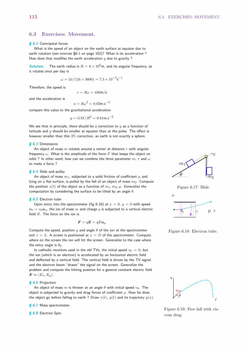
115 6.3. EXERCISES: MOVEMENT.
6.3 Exercises: Movement.
§ 6.2 Centripetal forcesWhat is the speed of an object on the earth surface at equator due to
earth rotation (see exercise §6.1 on page 102)? What is its acceleration ?How does that modifies the earth acceleration g due to gravity ?
Solution. The earth radius is R = 6× 10⁶m, and its angular frequency, asit rotates once per day is
ω = 2π/(24× 3600) = 7.3× 10⁻⁵s−1
Therefore, the speed isv = Rω = 440m/s
and the acceleration isa = Rω2 = 0.03m.s−2
compare this value to the gravitational acceleration
g = GM/R2 = 9.81m.s−2
We see that in principle, there should be a correction to g as a function oflatitude and g should be smaller at equator than at the poles. The effect ishowever smaller than this 3% correction, as earth is not exactly a sphere.
§ 6.3 DimensionsAn object of mass m rotates around a center at distance r with angular
frequency ω. What is the amplitude of the force F that keeps the object onorbit ? In other word, how can we combine the three parameter m, r and ωto make a force ?
§ 6.4 Slide and pulley
Figure 6.17: Slide
An object of mass m1, subjected to a solid friction of coefficient µ andlying on a flat surface, is pulled by the fall of an object of mass m2. Computethe position x(t) of the object as a function of m1,m2,µ. Generalize thecomputation by considering the surface to be tilted by an angle θ.
§ 6.5 Electron tubeUpon entry into the spectrometer (fig 6.18) at x = 0, y = 0 with speed
v0 = v0ux, the ion of mass m and charge q is subjected to a vertical electricfield E. The force on the ion is
Figure 6.18: Electron tube.
F = qE = qEuy
Compute the speed, position y and angle θ of the ion at the spectrometerexit x = L. A screen is positioned at x = D of the spectrometer. Computewhere on the screen the ion will hit the screen. Generalize to the case wherethe entry angle is θ0.
In cathodic monitors used in the old TVs, the initial speed v0 = 0, butthe ion (which is an electron) is accelerated by an horizontal electric fieldand deflected by a vertical field. The vertical field is driven by the TV signaland the electron beam “draws” the signal on the screen. Generalize theproblem and compute the hitting position for a general constant electric fieldE = (Ex,Ey).
§ 6.6 ProjectionAn object of mass m is thrown at an angle θ with initial speed v0. The
object is subjected to gravity and drag forces of coefficient ρ. How far doesthe object go before falling to earth ? Draw x(t), y(t) and its trajectory y(x).
Figure 6.19: Free fall with vis-cous drag.
§ 6.7 Mass spectrometer.
§ 6.8 Electron Spin.

CHAPTER 6. MECHANICS. 116
§ 6.9 Rockets.Consider a simplified rocket submitted only to the constant, vertical thrust
force FR and the gravity one Fg = −mg. At t = 0, when the thrust be-gins, v = 0. As the rocket advances, it consumes its fuel and its mass mdiminishes. Let us suppose that the mass decreases linearly
m(t) = m0 − αt
Compute v(t), and compare and draw it to the case where α→ 0.
§ 6.10 Air friction.For a car or a bicycle, the friction force is not linear in speed but quadratic
:Fν = −mv2
Which distance ` a mass m with initial speed v0 can travel in such a medium?
§ 6.11 Orbital speed.What is the necessary orbital speed of a satellite to keep it at distance r
from earth surface ? Where is the geostationary orbit ?
Solution. We know that the force necessary to keep an object rotating atdistance r at constant angular frequency is
Fc = ma = mv2/r
This force provides from the earth gravitation. Therefore, we must have
GMm/r2 = mv2/r
orv =
√GM/r
When the orbit is geostationary, the angular frequency of the satellite isthe same as for the earth ω = 7.3× 10⁻⁵s−1. As v = rω, we must have
r2ω2 =GM
r
Given that G = 6× 10⁻¹¹S.I. and M = 6× 1024kg, we have
r ≈ 4.1× 10⁷m
or 41000 km. Removing the earth radius, the satellite must be at 35000 kmabove us.
6.2
§ 6.12 The Milikan ExperimentIn 1909, Milikan and Fletcher performed the first experiment that de-
termined the charge of an electron9. It consists of observing (under a low 9 The experiment is known as the“Milikan” experiment alone becausehe excluded Fletcher (his PhD stu-dent) from co-authoring the scientificarticle. Milikan (alone) was awardedthe Noble prize.
magnification microscope) the fall of a charged oil drop under uniform electricfield and measuring its limit speed. For a drop of radius r, the equation ofmotion is
mdv
dt= −g(4πr3/3) (ρoil − ρair)− νv + qE
where ρ is the density, ν the viscous drag experiment and E the electric field.Comment the various terms of the above equation, solve it, find the speedlimit v0 when q = 0 ; vq when q 6= 0 and finally ∆(q) = vq − v0.
Milikan and Fletcher found that only discrete values for ∆(q) exist. Theyconcluded that charge must be quantified. The smallest value for ∆(q) intheir experiment led to deduce e.

117 6.3. EXERCISES: MOVEMENT.
§ 6.13 Cross product.For two vectors u = (x1, y1, z1) and v = (x2, y2, z2), the cross product is
defined as a vector with coordinates
w = u∧ v = (y1z2 − y2z1, z1x2 − x1z2,x1y2 − x2y1)
Its geometrical interpretation is a vector that is perpendicular to both u and vwith a magnitude
w = uv sin θ
where θ is the angle from u to v. In particular, if two vectors are co-linear,their cross product is zero. In particular, u∧u = 0.1. Demonstrate that
w = u∧ v + u∧ v
2. Let us define the angular momentum of a movement by
L = mr ∧ v
where r is the position of the object and v its speed. Demonstrate that ifthe force applied to the object is central, i.e.
F (r) = f(r)r
thendL
dt= 0
in other word, the angular momentum is conserved if the force is central.

CHAPTER 6. MECHANICS. 118
6.4 Kinetic energy, work, power.
Computing the trajectory of the particle as a function of the forceinvolves solving a differential equation, and the details of how you dothese kind of computations takes many chapters in any textbook onmechanics. Some quantities however can be computed by a simpleintegration. Consider again relation (6.8) where we have taken thescalar product of both sides with the vector v:
Definition 7 The kinetic energy Tof a particle is defined by
T = (1/2)mv2
. The work W provided to a parti-cle by a force F is
W =
ˆC
F.dx
where C is the trajectory of theparticle.
mv.dvdt
= F.v (6.25)
Note thatv.dv = (1/2)d (v.v)
and vdt = dx by definition. So we can rewrite relation (6.25) as
12md (v.v) = Fdx (6.26)
OK, we just shuffled some quantities around, but by doing that, wehave obtained a very useful relation indeed. The quantity
T =12mv
2
is called the Kinetic energy of the particle. Note that unlike themomentum, it is a plain scalar (not vectorial) quantities and it isrelated to the square of the speed. The quantity
Definition 8 The infinitesimalchange in kinetic energy T of aparticle is equal to the infinitesimalwork done by the force: defined by
dT = dWdW = Fdx (6.27)
is called the infinitesimal work of the force. Now, let us stress theimportance of relation we have obtained: A particle, originally atposition x1 and speed v1 is acted upon by a force F and reachesposition x2 and speed v2 , following the trajectory C. The changein the kinetic energy is equal to the amount of work provided to theparticle.
T2 − T1 = W =
ˆC
Fdx (6.28)
As you can observe, the time has been formally eliminated fromthe equations: we only need to know the trajectory followed by theparticle to get the change in its speed. These relations do not involvevectorial computations, but just plain scalars.
§ 6.14 The magnetic force FB exerted by a magnetic field on a chargedparticle is always perpendicular to the speed of the particle. What changes inthe kinetic energy does it produce ?
Solution. From the definition, we know that FB .v = 0, so the infinitesimalwork
dW = FB .dx = FB .vdt = 0
And therefore, there is no change in the kinetic energy of the particle. Notethat this does not mean that the particle does not change its (vectorial)speed; just that the magnitude of the speed does not change. For a magneticfield B, the magnetic force is F = qv×B. Let us suppose that the magnetic

119 6.5. POTENTIAL AND TOTAL ENERGY.
field is along the z axis, B = Bez . Then, the fundamental law (6.8) in thiscase reads
dvxdt
= (Bq/m)vy
dvydt
= −(Bq/m)vx
noting κ = Bq/m, and deriving one more the above equations, we find that
d2vαdt2
+ κ2vα = 0 (6.29)
where α = x, y. This is a simple second order ODE which we know how tosolve. One more integration shows that the particle describes a helix along thez axis.
§ 6.15 Use the full solution (6.29) of §6.14 to show that the kinetic energydoes not change upon the action of a magnetic force.
6.4.1 Power.
We saw that the (infinitesimal) change in kinetic energy dT is equalto the work done by the (infinitesimal) force dW = Fx (definition 8).This statement however does not contain any information about howfast this change happens. We could trivially divide both side by dtand write
dT
dt=dW
dt
and say that the rate of change in kinetic energy (dT/dt) is equal tothe rate of the work (dW/dt ) done. The rate at which the work isdone is called the Power P :
P =dW
dt= Fv
The unit of the power is J/s which is called a Watt (W).If you shutdown the motor of your car on the highway, your speed
will drop because of the friction forces. At each time, the power ofthese forces is the force multiplied by the speed. If the friction forcesare of the form F = −ρv, then the power of these forces at each timeis
Pfrict = −ρv2 (6.30)
and is of course negative as you decrease your speed. In order tokeep a constant speed, the motor has to compensate for this loss byproviding an equivalent positive power. You could say that you aredissipating this much energy per second into the environment.
6.5 Potential and total energy.
Relation (6.28) is very nice, but it can get much nicer if ...Very often, the force which is exerted upon of particle is only a
function of the position of the particle F = F(x). The gravitationalforce, or the electric one, are only function of the distance separat-ing the two objects (and their mass or charge, which don’t changeusually).

CHAPTER 6. MECHANICS. 120
To be honest, this is the case of all the forces in nature. Some-times however, the number of particles interacting is so big that thisformulation becomes unnecessary complicated. A particle submittedto friction is indeed interacting with all the molecules of the fluidaround it (which are also interacting among themselves), so the forceexerted on this particle is function of its position and those of all theothers which we don’t know. In these various cases, we may use adhoc forces of more complicated form F = F(t, x, v), which capturethe action of the numerous other particles present, in which we arenot interested. The friction force at small speed for example takesthe form of F = −νv, where the friction coefficient ν is function ofthe properties of the surrounding fluids.
For this lecture however, we restrict ourselves to the simple caseswhere we can write F = F(x). Vectorial notations can be confusing,so let us first develop all the concepts in a one dimensional world(the position along a straight highway for example), knowing thateverything extends naturally to three-dimensional world.
The force F = F (x) can be written as the derivative of anotherfunction U(x):
F (x) = − d
dxU(x)
We say that the force is conservative. The function U is called thepotential energy of the particle, for reason we’ll shortly explain.Now, when the particle moves from position x1 to position x2, theamount of work is
W =
ˆ x2
x1
Fdx
=
ˆ x2
x1
−U ′(x)dx
= − (U(x2)−U(x1))
We see that in this case, we even don’t need to perform any integra-tion, the value of the potential energy at end points is enough. Wecan now rewrite relation (6.28) in an even simpler form:
Definition 9 Total energy The sumof the kinetic and potential energy
E = T + U
is called the total energy of aparticle.
T2 + U2 = T1 + U1 (6.31)
The quantity E = T + U is called the total energy of the particle.The relation (6.31) shows that when a particle is submitted to a con-servative force, its total energy doest not change as it is conserved.What it looses in kinetic energy it gains its potential energy, andvice et versa.
The above concepts of potential and total energy extends natu-rally to three dimensions, with a small addition. Let us call the threecoordinates by x, y, z and the component of the force by Fx,Fy,Fz.A potential energy exists if there is a function U(x, y, z) such that
Fα = −∂U∂α
where α = x, y, z. This is written in vectorial notation as
F = −∇U

121 6.5. POTENTIAL AND TOTAL ENERGY.
where the symbol ∇ is called the gradient. As surprising as it wouldseem, we cannot always find a potential for any force10. Fortu- 10 This is a complication of having
more than one dimension.nately11, all fundamental forces of nature derive from a potential. 11 We do live in a nice world.
CHAPTER 6. MECHANICS. 122
6.6 Exercises : Energy
§ 6.16 gravity 1. Around the surface of the earth, the gravitational force isF = −mg ez . Show that the gravitational potential is
U = mgz
§ 6.17 spring. Let us take the equilibrium position of an atom in a crystal asthe origin. The force exerted on this atom by all others in the crystal can bemodeled by
Fα = −kαα
where α = x, y, z and kα are microscopic coefficients depending on thematerial. Show that the potential energy of this atom is
U =12(kxx
2 + kyy2 + kzz
2)In general, potential energies of the form U = kx2 are called harmonic
potentials. This is for example the potential energy of a spring for smalldeformations.
§ 6.18 gravity 2. The general form of the gravitational force exerted by earthon a object of mass m (say a satellite ) is
F = GMmurr2
where r =√x2 + y2 + z2 is the distance to the center of the earth, and ur
is the unit vector from the satellite pointing toward the center of the earth.Show that the potential is
U = −GMm/r
§ 6.19 Escape velocityWhat is the minimum initial velocity of an object on earth necessary to
escape earth’s gravitational attraction ?
Solution. The initial energy of the object is
E1 = (1/2)mv20 −GMm/R
where R = 6× 10⁶m is the earth radius. When the object escapes completelyearth, its speed is 0 and its position R = ∞. Therefore its energy is E2 = 0.We must then have E1 = 0 or
v0 =√
2GM/R
As G ≈ 6× 10⁻¹¹S.I and M ≈ 6× 1024kg, the escape velocity is v0 ≈11km/s. We saw in exercise §6.2 on page 115 that around 440m/s of thisspeed can come from the earth rotation if we are close to equator.
Compare this speed to the one needed to position a satellite on the geosta-tionary orbit (exercise §6.11, page 116).
§ 6.20 Maximum heightWhat is the maximum height of an object thrown with initial velocity v0 at
an angle θ ?
Solution. We first note that as there is no force in horizontal direction, themomentum (and the speed) in this direction is conserved : vx(t) = vx,0 =
v0 cos θ. At maximum height h, vy = 0. Using conservation of energy, wemust have
(1/2)mv20 = (1/2)mv2
0 cos2 θ+mgh
orh =
v20
2g(1− cos2 θ
)

123 6.6. EXERCISES : ENERGY
§ 6.21 Roller coasterAn object of mass m, with no initial velocity, slides along a roller coaster
beginning at the top. Determine its speed at positions 1,2,3,4 where its heightis y1,...y4 and at the exit point(figure 6.20).
Figure 6.20: Roller coaster§ 6.22 sliding
An object of mass m, with no initial velocity, slides along a circle of radiusr beginning at the top of the circle. At which height will it detach from thecircle ?
Solution. the necessary force to keep an object on rotation is
Fc = mv2/r
and this force is provided by the projection of gravitation on the circle radius
Figure 6.21: Sliding along acircle
Fg = mg cos θ
At the beginning of the slide, v ≈ 0 and Fg ≈ mg, therefore gravitationis enough to keep the object on the path. However, as the object slidesdown, Fc increases and Fg decreases ; when they are equal, gravitation isnot enough anymore. This happen if the speed reaches
v∗2 = gr cos θ (6.32)
We shall therefore compute at which angle θ the speed reaches this value. Atthe beginning of the slide, y0 = r
E1 = 0 +mgr
when the object reaches height y with speed v = v(y),
E2 = (1/2)mv2 +mgy
and therefore the speed, as a function of y is
v2 = 2g(r− y) = 2gr(1− cos θ) (6.33)
Comparing expressions (6.32) and (6.33), we find that the critical angle issuch that
cos θ = 2/3
ory∗ = 2r/3
§ 6.23 PendulumAn object of mass m is attached to a fix point by a rope of length ` and
restricted to stay in a plane (figure 6.22). Find the equation of its movement.
Solution. Even though the movement is in two dimension, we only haveone degree of freedom, the angle θ with the vertical. The coordinates of theobjects are
Figure 6.22: Pendulumx = ` sin θ ; y = `(1− cos θ)
if the angle is varied by dθ, the x, y coordinates vary by
dx = ` cos θ.dθ ; dy = ` sin θ.dθ
and therefore the amplitude of the speed is v2 = `2θ2. On the other hand,the potential energy is U = mgy = mg(1− cos θ). The total energy, which isconserved, is therefore
E = (1/2)m`2θ2 +mg(1− cos θ)

CHAPTER 6. MECHANICS. 124
Where θ = θ(t) is the only variable. Let us derive in respect to time:
0 = m`2θθ+mg sin θ.θ
and simplifying the above relation by mθ, we find
θ+ (g/`) sin θ = 0
If the amplitude θ 1, then sin θ ≈ θ ; setting ω2 = g/`, we have
θ+ ω2θ = 0
which is the harmonic oscillator equation for θ. We know that the generalsolution is of the form
θ(t) = A cos(ωt+ φ)
where A and φ are obtained from initial conditions.
§ 6.24 Spring and gravityA spring of constant k is disposed vertically, and an object of mass m is
attached at its end. The equilibrium position of the spring corresponds toy = 0. At time t = 0, the object is at y = 0 and is released with no initialspeed (v = 0).1. What are the forces exerted on the object ? Deduce and compute the
potential energy U of the object as a function of its position y. DrawU(y).
2. Using the conservation of energy, compute the lowest position h that theobject will reach.
Figure 6.23: Vertical spring.
3. Using the conservation of energy, compute the speed v1 of the objectwhen y = h/2.
4. We can suppose that the object is oscillating between position y = 0 andy = h, and therefore its position as a function of time is given by
y(t) = (1− cos(Ωt)) h/2 (6.34)
where the oscillation frequency is to be determined. Compute the time t∗at which the object reaches h/2 for the first time and its speed v1 at thistime by using directly equation (6.34).
5. Compare expression of v1 found in questions (3) and (4) and determineΩ as a function of m and k. Is that coherent with what you know fromharmonic oscillator ?

125 6.7. EQUILIBRIUM.
6.7 Equilibrium.
6.7.1 Basic concepts.
An object is at equilibrium when is does not move. From the New-ton principle ma = F, we deduce that an object is at equilibrium ifno force is applied to it. If an object is subject to multiple forces Fi,we deduce then that at equilibrium, the sum of these forces shouldbe zero: ∑
i
Fi = 0 (6.35)
If some of the forces depend on the position xof the object, relation(6.35) is an equation determining the equilibrium position xeq.
Figure 6.24: A constant forceand the spring restoring forceon a object.
For example, consider a one dimensional object attached to aspring and submitted to a constant force F (figure 6.24). The restor-ing force applied by the spring if Fs = −kx, where k is the springconstant and x the displacement. As the force displaces the objectsand |x| increases, the restoring force by the spring also increases.There is a position x where these two forces compensate exactly:F + Fs = 0 and this is where x = xeq, where
xeq = F/k
Figure 6.25: An object sittingon a plane.
Computing the equilibrium is more complicated when an objectis subject to geometrical constraint. For example, consider an objectsitting on a table (figure 6.25). There is the vertical force of thegravity Fg = −mg ; as the object is not moving, we deduce that thetable is also exerting of force FR on the object that cancel exactlythe gravity. Therefore, this reaction force must be
FR = mg
Figure 6.26: A pendulum sub-jected to a horizontal force F.
The problem with these forces of the reaction is that they arenot known a priori. They are such that the geometric constraint isrespected. Consider now the more tricky problem of the pendulum :a mass m is attached to a fixed point by a massless rod of length `.The mass is subjected to a (known) constant horizontal force F andalso to gravitation Fg = −mguy. There is also the reaction forceFR applied by the rod to the object. The problem is, we don’t knowthe value of this force, we only know that it must be directed alongthe rod (why ?). Writing that the sum of the forces are zero at theequilibrium position θ and projecting on the two axes, we must have
F − FR sin(θ) = 0−mg+ FR cos(θ) = 0
We see here that the above relation has two unknowns and tworelations. Not only we have to find the equilibrium position θ, butalso the amplitude of the reaction force FR about which we reallydon’t care. In this case, the reaction force can be easily eliminatedand we have
tan θ = F
mg

CHAPTER 6. MECHANICS. 126
In many slightly more complicated cases, we cannot that easily getrid of the reaction force computation.
6.7.2 Forgetting the forces of reactions.
When geometrical constraint are present, we saw above that we haveto take into account reaction forces. The only purpose of the reac-tion forces is to compel the object to respect the constraint12. If the 12 In mathematics, these are known
as Lagrange multipliersobject moves in a direction dr compatible with the constraints, thisdirection is necessarily orthogonal to the reaction forces FR (take theexample of the pendulum). Now, suppose that an object is subjectto various forces F and some reaction forces FR. At equilibrium, wemust have
F + FR = 0
Let us move from this direction by a displacement dr compatiblewith the constraints and consider the Work dW done by this dis-placement:
dW = (F + FR) .dr
Because the displacement is compatible, we must have, withoutcomputing the reaction forces explicitly, FR.dr = 0. On the otherhand, as the sum of the forces are zero, we also must have
F.dr = 0 (6.36)
And this last relation which does not imply the reaction forces isenough to determine the equilibrium principle. This is known as theprinciple of virtual work: At equilibrium, the work for a compatibledisplacement is zero13. 13 In other words, If the forces derive
from a Potential, the equilibriumcorresponds to the minimum of thepotential.
As an example, consider the pendulum (fig 6.26) again. Let ussuppose that we are at equilibrium, and let us make a displacementof the angle dθ. This is obviously a compatible displacement as itdoes not change the distance between the mass and the fixed point.The displacement dx and dy are
dx = ` sin θ ; dy = ` cos θ
and the work for this displacement is
dW = Fdx−mgdy = `(F sin θ−mg cos θ) = 0
and therefore,tan θ = F
mg
We see here that the reaction forces are automatically taken care ofand never spoken about. Few exercises will familiarize us with thisincredibly elegant method.
6.7.3 Torque and solid objects.
Consider a rigid assembly of some points Pi subjected to forces ap-plied to them. We want to establish the condition under which the
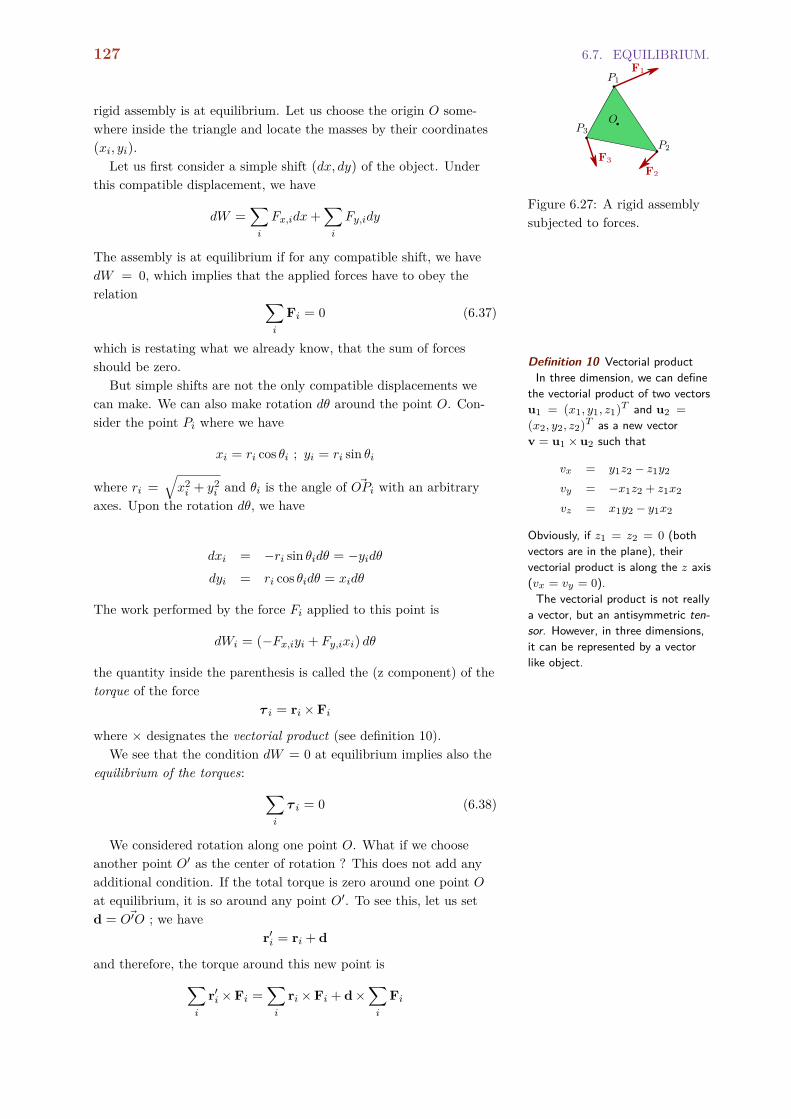
127 6.7. EQUILIBRIUM.
rigid assembly is at equilibrium. Let us choose the origin O some-where inside the triangle and locate the masses by their coordinates(xi, yi).
Figure 6.27: A rigid assemblysubjected to forces.
Let us first consider a simple shift (dx, dy) of the object. Underthis compatible displacement, we have
dW =∑i
Fx,idx+∑i
Fy,idy
The assembly is at equilibrium if for any compatible shift, we havedW = 0, which implies that the applied forces have to obey therelation ∑
i
Fi = 0 (6.37)
which is restating what we already know, that the sum of forcesshould be zero.
But simple shifts are not the only compatible displacements wecan make. We can also make rotation dθ around the point O. Con-sider the point Pi where we have
xi = ri cos θi ; yi = ri sin θi
where ri =√x2i + y2
i and θi is the angle of ~OPi with an arbitraryaxes. Upon the rotation dθ, we have
Definition 10 Vectorial productIn three dimension, we can define
the vectorial product of two vectorsu1 = (x1, y1, z1)
T and u2 =
(x2, y2, z2)T as a new vector
v = u1 × u2 such that
vx = y1z2 − z1y2
vy = −x1z2 + z1x2
vz = x1y2 − y1x2
Obviously, if z1 = z2 = 0 (bothvectors are in the plane), theirvectorial product is along the z axis(vx = vy = 0).The vectorial product is not really
a vector, but an antisymmetric ten-sor. However, in three dimensions,it can be represented by a vectorlike object.
dxi = −ri sin θidθ = −yidθdyi = ri cos θidθ = xidθ
The work performed by the force Fi applied to this point is
dWi = (−Fx,iyi + Fy,ixi) dθ
the quantity inside the parenthesis is called the (z component) of thetorque of the force
τ i = ri ×Fi
where × designates the vectorial product (see definition 10).We see that the condition dW = 0 at equilibrium implies also the
equilibrium of the torques: ∑i
τ i = 0 (6.38)
We considered rotation along one point O. What if we chooseanother point O′ as the center of rotation ? This does not add anyadditional condition. If the total torque is zero around one point Oat equilibrium, it is so around any point O′. To see this, let us setd = ~O′O ; we have
r′i = ri + d
and therefore, the torque around this new point is∑i
r′i ×Fi =∑i
ri ×Fi + d×∑i
Fi

CHAPTER 6. MECHANICS. 128
The first term on the right hand side is zero because of relation(6.38), and the second one because of relation (6.37).
More over, as any displacement can be decomposed into a shiftand a rotation, relations (6.37-6.38) are the only necessary and suffi-cient condition for equilibrium.

129 6.8. EXERCISES: EQUILIBRIUM.
6.8 Exercises: Equilibrium.
§ 6.25 Simple PendulumConsider again the simple pendulum of figure 6.35. This time however,
we consider not a horizontal force, but a force with arbitrary direction F =
(fx, fy). Show that the equilibrium position is
tan θ = fxmg− fy
Discuss the case fy = 0 and fx = 0 : is it possible to have an equilibrium po-sition other than θ = 0 when fx = 0 ? What is the nature of this equilibrium?
Among all the forces that allow an equilibrium position θ∗, find the force Fwith minimal amplitude and show that, for this minimal force, the ratio fy/fxmust be tan θ∗.
§ 6.26 leverFind the amplitude of the vertical force for the lever (with the fixed point
O) to be at equilibrium (figure 6.28).
Figure 6.28: A lever.Solution. We have two external forces : the gravity Fg = −mguy exertedon the mass (point P2 ) and the force F = fuy exerted on the other endof the lever (point P1). We have to compute the work of both forces for acompatible displacement. These displacements are rotation around origin,which we can refer to be the angle θ between the horizontal axis and point P2for example. Upon a variation dθ, the point P2 is moved by
dx2 = −`2 sin θ ; dy2 = `2 cos θdθ
The angle with the point P1 is π + θ and therefore
dx1 = `1 sin θ ; dy1 = −`1 cos θdθ
The infinitesimal work of these forces is
Figure 6.29: Ladder along awall
dW = Fg.dr2 + F.dr1
= (−`2mg− `1f) cos θ.dθ
To have equilibrium, we must have
f = − `2`1mg
We see that the force has to correct sign, and its amplitude is mg, amplifiedby the lever factor `2/`1.
§ 6.27 Ladder
Figure 6.30: Compound pendu-lum.
A massless ladder of length L is set with an angle θ along a wall (figure6.29). An object of mass of m is attached at the middle of the ladder. Com-pute which horizontal force F = Fux we have to exert at the bottom of theladder in order to keep it in equilibrium. Discuss specifically the cases θ ≈ 0and θ ≈ π/2.
§ 6.28 compound pendulumFind the equilibrium position of the two compound pendulum of figure
6.30.
§ 6.29 Equilibirum on a curved plane.Figure 6.31: Equlibrium alonga curve.
Find the equilibrium position of the an object of mass m submitted to ahorizontal force restricted to remain on the curve C : y = f(x) ( figure 6.31).Find the result when y = A sin(x). Does an equilibrium position always exist?

CHAPTER 6. MECHANICS. 130
§ 6.30 Cylinder (advanced)A mass less cylinder, with a mass m attached to point of its surface, is
restricted to remain on a horizontal plane. Find the equilibrium position ofthe cylinder subjected to a horizontal force applied to its center (figure 6.32).There is no slipping, only rotation.
Figure 6.32: Cylinder equilib-rium.
Solution. We must note that a rotation of angle θ induced a horizontalmovement of x1 = −rθ for the center of the main cylinder. The movement ofthe mass is given by
x2 = x1 + r sin θ ; y = −r cos θ
the total work for an infinitesimal displacement is therefore
dW = −Frdθ−mgr sin θdθ
and the equilibrium angle θ∗ is such that
sin θ∗ = − F
mg
We see that no equilibrium is possible if |F | > mg : the cylinder will roll inthis case.
§ 6.31 Cylinder II.Can the same cylinder be at equilibrium on an inclined plane (figure 6.33
)? Is there a critical angle that will make that impossible 14? 14 For an extension of this exercise tounderstand granular materials, seethis article
Figure 6.33: Cylinder on aninclined plane.
§ 6.32 Torque.To be added.

131 6.9. THE LAGRANGIAN FORMULATION.
6.9 The Lagrangian formulation.
6.9.1 Introduction.
Consider a plane (t,x) and consider all the trajectories x(t) whichlead from a point P0 = (t0,x0) to a point P1 = (t1,x1). We canassociate a cost to each trajectory. For example, we would define thecost (a number) as
Figure 6.34: Few trajectoriesleading from (t0,x0) to (t1,x1).Given a global cost, there isone trajectory which is opti-mum relative to this cost.
S [x(t)] =
ˆ t1
t0
(x′(t)
)2dt
at each point along the trajectory, we compute a local cost, for ex-ample the square of the slope, and then sum all this local costs tocompute the global cost of a trajectory. The cost can have any form,such as for example
S[x(t)] =
ˆ t1
t0
[(x′(t)
)2+ f (x(t))
]dt
Generally, we will write
S[x(t)] =
ˆ t1
t0
L(x′,x, t)dt
where L is the local cost function. We have restricted the treatmentto local costs which depend only on the slope and the position, butthis can be easily generalized further. The local cost L is often calledthe Lagrangian.
Is there a unique trajectory xbest(t) which has the lowest possiblecost ? The answer is yes15 and we have indeed a tool which given 15 Caution needed, but very often
yes.the Lagrangian, enables us to compute the best trajectory. Thistool was generally derived by Euler back in the ~1720’s: given L, wecan find a differential equation relating x′(t) and x(t) for the besttrajectory.
Now consider a one dimensional world where the position ofthe particle is x(t). The kinetic energy of the particle at time t isEc = (m/2) (x′(t))2 and the potential energy of the particle isEp = f (x(t)). The fundamental law of mechanics16 states that the 16 The relation between minimum
trajectories and mechanics was madeclear by Lagrange in the ~1770’s ;the differential equations followedby the trajectory is called the Euler-Lagrange equations.
trajectory followed by the particle is the one which extremizes theLagrangian L = Ec −ET .
This is a kind of minimum principle we will encounter many timesand it is the most fundamental way of formulating the law of me-chanics17. It can be generalized to any dimension and any number 17 and uniting mechanics and geome-
tryof particles, and generalizes to other branches of physics such aselectrodynamics and quantum mechanics. In fact, all fundamentalphysical theories are formulated through the Lagrangian approach.The Newton equations of motion are just a simple consequence ofthis general minimum principle. The interested reader is referred toa more detail textbook on mechanics to learn the power and beautyof this formulation.

CHAPTER 6. MECHANICS. 132
6.9.2 Why Lagrangian mechanics ?
As we said above, the Lagrangian mechanics is the most natural andelegant ways of formulating the laws of physics. But from a practicalpoint of view, is it worth it ? The answer is a definite yes and this iswhy in the first place, this method became so popular18. 18 The Newtonian mechanics was
formulated in the ~1680 ; the La-grangian ones in the ~1760.
Figure 6.35: The simple pendu-lum
In fact, the Newtonian Mechanics is bad at formulating prob-lems where there are geometrical constraints. We will study belowa simple example (without solving it) to show why it is so bad, andthen go to the Lagrangian mechanics and see how easily the sameproblem can be solved.
For example, consider the very simple pendulum (figure 6.35),where the mass m is attached by a rigid, massless rod of length ` toa fixed point. What are the forces applied to the mass ? There isof course the force Fg of the gravity, with amplitude mg and in thevertical direction. But there is also a force Fr applied by the rod onthe mass. This force must be such that, when writing the equationof movement mr = Fg + Fr , the mass must always stay at distance` of the fixed point. Newton thus stated that for each force appliedby an object 1 to an object 2, there is a counter-force (the reactionforce) of equal amplitude and in the reverse direction applied bythe object 2 to the object 1. It is not hard to deduce that, for thependulum, the amplitude of the force Fr must be mg cos θ and itsdirection parallel to the rod. We then have to decompose this forcealong to two axes (being careful with the signs ) :
mx = −mg cos θ sin θmy = −mg(1− cos2 θ)
keeping in mind that θ varies in time and is a function of x and y.This is obviously a hard differential equation to solve. The trick isto write x = ` sin θ, and therefore x = `θ cos θ − θ2 sin θ ; deducea similar expression for y, note that then x cos θ + y sin θ = `θ andfinally obtain an equation for θ:
θ = −g`
sin θ (6.39)
§ 6.33 Demonstrate relation (6.39) for the pendulum, using the Newtonianmechanics.
We did all that to obtain finally an equation (which is simple)for the only quantity, θ, that describes the movement of pendulum!An other classical way of obtaining the pendulum equation is tointroduce a rotating frame pointing to the object. Students learn tomanipulate the messy algebra of moving frames during the first yearof university with some pain and we totally avoid the subject here.As we will see below, the Lagrangian mechanics allows us to simplyobtain equation (6.39) without introducing the reaction forces, andwithout doing any trick, in a systematic way.

133 6.9. THE LAGRANGIAN FORMULATION.
6.9.3 The Euler-Lagrange equation.
The first step in Lagrangian mechanics is to enumerate the relevantquantities of the problem which are called degree of freedom. In thependulum example, the degree of freedom is the angle θ. Let ussuppose that we have a particle in a one dimensional world whereits coordinate is x, its kinetic energy T = mx2/2 and its potentialenergy is U(x). The Lagrangian is a function of both the speed andthe position of the particle and is defined as
L(x,x) = T −U
for the simple example above, we have
L(x,x) = m
2 (x)2 −U(x)
The Euler-Lagrange equation deduces the law of movements fromthe Lagrangian:
d
dt
(∂L∂x
)−(∂L∂x
)= 0 (6.40)
It looks formidable, but in reality, it is quite simple.The Lagrangian is a function of two variables : the speed x and
the position x. The first step is to look at x as an independent vari-able and derive L in respect to this variable. This is the meaning ofthe expression ∂L/∂x. To get use to this derivation, give anothername to x, for example v, write again the Lagrangian, derive in re-spect to this variable and then restore the name. For example, forour simple example,
L = (m/2)v2 −U(x)(∂L∂v
)= mv(
∂L∂x
)= mx
This is the hardest part. Now that we have ∂L/∂x, we derive itas a function of time. For our example,
d
dt
(∂L∂x
)=
d
dt(mx) = mx
So far, we have computed the first part of the E-L equation. For theremaining part, again we treat x and x as independent variables andderive the Lagrangian as a function of x this time. For our example,
L = (m/2)v2 −U(x)(∂L∂x
)= −U ′(x)
If now we group all the terms, we get the E-L equation for our sim-ple example:
mx+ U ′(x) = 0
And if we recall that the force is defined as −U ′(x), we get the New-ton law’s of movement mx = F .

CHAPTER 6. MECHANICS. 134
The Euler-Lagrange equation is equivalent to the Newton equa-tion! Of course, this should be true or else there would be no worthin the E-L equation.
Let us now consider the more complicated case of the pendulum(figure 6.35). We have only one degree of freedom, and let us chooseθ, the angle with the vertical axis, as this degree:
x = ` sin θ ; y = −` cos θ
The kinetic energy is
T =m
2(x2 + y2)
=m`
2(θ)2
The potential energy is
U = mgy = −mg` cos θ
We see here the crucial part of the Lagrangian formulation: oncethe degrees of freedom have been chosen, we express kinetic andpotential energy only as function of the degrees of freedom. Now, theLagrangian L = T −U is
L =m`
2(θ)2
+mg` cos θ
and we can do the E-L derivation:
∂Lθ
= m`θ
d
dt
(∂Lθ
)= m`θ(
∂Lθ
)= −mg` sin θ
and therefore, the E-L equation is
m`θ = −mg` sin θ
which is the equation (6.39) we had obtained the hard way.If we have more than one degree of freedom, say n, the La-
grangian is of the form
L(x1,x1, x2,x2, ..., xn,xn)
and we apply the E-L to each degree of freedom and write n equa-tions :
d
dt
(∂L∂(xi)
)−(∂L∂xi
)= 0 i = 1, 2, ...,n
Let us apply that to the movements of planets around the sun. Thisis the example which Newton treated (the hard way) and hencebegan the advent of the modern science.

135 6.9. THE LAGRANGIAN FORMULATION.
6.9.4 Planetary movement.
We suppose that the sun, with mass M , is the center of our coordi-nated. We suppose first that the movement takes place in a planeand deduce the E-L equation. We will then show why the movementis in a plane which will illustrate how we obtain conserved quantities(such as energy, ..) in mechanics.
For the movement of the planet of mass m around the sun, weuse the cylindric coordinates r and θ. These are related to Cartesiancoordinates through
x = r cos θ ; y = r sin θ
The kinetic energy of the planet is
T =12mv
2 =12m
(x2 + y2)
=m
2((r cos θ− rθ sin θ)2 + (r sin θ+ rθ cos θ)2)
=m
2(r2 + r2θ2)
The potential energy of the planet is
U = −kmr
where k is a constant19. So the Lagrangian is, up to the constant m, 19 equal to MG, where G is thefundamental constant of gravitation.
L(r, r, θ, θ) = 12(r2 + r2θ2)+ k
r
Let us now derive the E-L equation. For the variable r we have
∂L∂r
= r ; ddt
(∂L∂r
)= r ; ∂L
∂r= rθ2 − k
r2
and we obtain the first equation of movement:
r− rθ2 +k
r2 = 0 (6.41)
For the variable θ we have∂L∂θ
= r2θ ; ∂L∂θ
= 0
and the second equation of movement is
d
dt
(r2θ)= 0 (6.42)
And this is it, we have the law of movement! We have two variablesand two differential examples, so we can solve them, at least numeri-cally. We can also solve them exactly with a little more effort.
For example, from equation (6.42), we have the conservation ofr2θ
r2θ = C (6.43)
where the constant C is found from the initial conditions. Thusθ = C/r2 and the relation (6.41) transforms into
r− C
r3 +k
r2 = 0 (6.44)

CHAPTER 6. MECHANICS. 136
This is just an ordinary differential equation in one variable and wenote that it derives from
12 (r)2 +
C
2r2 −k
r= D (6.45)
where D is another constant found from the initial conditions. Thisis a nice, separable equation which can be solved by the usual tech-niques we saw in subsection 2.2.6.
We can however note that we can combine equations (6.43,6.45)to obtain directly a relation for dθ/dr, by eliminating the time vari-able. By solving this equation, we obtain the orbit of the planet,which happens to be an ellipse. The details of this problem will bedealt with in the exercises.
6.9.5 Mechanics of solid objects.
Until now, we have only studied the mechanics of point masses, i.e.objects with small spatial extensions to be considered as points. Thisis of course an approximation and for real life objects, we have to gobeyond this approximation.
Let us first consider two point mass m1 and m2 linked by arigid rod of length `. We will here consider only movements in theplane20. If the two point were not linked, we would need 4 coordi- 20 A more advanced course in me-
chanics is needed for 3D movements.The concepts are similar in 3D, butthe equations are too messy for theselectures.
nates (x1, y1) and (x2, y2) to describe them. Because of the geomet-ric constraint however, we need only 3 numbers.
Let us choose a point O = (x, y) inside the rod and call `1 and `2the distance from this point to the two masses (`1 + `2 = `). If wecall θ the angle the rod makes with an axis (say the horizontal axes),we have
x1 = x+ `1 cos θ ; y1 = y+ `1 sin θx2 = x− `2 cos θ ; y2 = y− `2 sin θ
The three number (x, y, θ) are enough to describe the system. Upona change of (dx, dy, dθ), the change in coordinates of the two pointsare
dx1 = dx− `1 sin θdθ ; dy1 = dy+ `1 cos θdθdx2 = dx+ `2 sin θdθ ; dy2 = dy− `2 cos θdθ
and the kinetic energy of the system is
T =m12(x2
1 + y21)+m22(x2
2 + y22)
=m12(x2 + 2`1 (−x sin θ+ y cos θ) θ+ `21θ
2)+
m22(x2 + 2`2 (x sin θ− y cos θ) θ+ `22θ
2)to continue...

137 6.10. EXERCISES: LAGRANGIAN.
6.10 Exercises: Lagrangian.
• Before real examples, create familiarity with E-L derivationthrough douzen of (more or less) artificial examples.
• The double pendulum ;
• pendulum with the fixation point free on a curve ;
• parametric oscillation ;
• pendulum with the fixation point vertically oscillating ;
• the brachistochrone ;
• point attached to a mass less cylinder ;
• detail study of planets ;
• Electromagnetic interaction, constant magnetic field as a particu-lar case.

CHAPTER 6. MECHANICS. 138
6.11 Advanced topics: Relativity.
Consider a train travel. You get in the train at 10:00 AM. Whenyou get into the train, you check your watch and the train station’sclock: they both indicate 10:00AM. After the travel, when you getout of the train, you again check your watch and compare it to thestation’s clock: surprise, there is a mismatch now between the twotime systems!
Figure 6.36: The clock insidethe train retards compared tothe train station’s clock.
Of course, for normal train travel, the mismatch is so small thatyou wouldn’t be able to really observe it. However, back in the1970’s, two scientists did the same experiment by taking commercialairplanes around our planet. Before the beginning of the journey,they synchronized two atomic (very precise) clocks and took onewith them around the world. At they return, they compared againthe two clocks and found a difference.
Around 1900, scientists had performed different experiments,similar in spirit to the travel experiment described above, whichcouldn’t be explained by the notion of an absolute time bathing allof the universe. The main conclusion of these experiments was thatthe speed of light is always the same, whatever the condition of theexperiment. More precisely, suppose that you are in a train movingat constant speed. No physical experiment done inside the trainwill allow you to determine whether you are moving (and at whichspeed) or not compared to the train station. This is called relativityprinciple.
Einstein first, and others (Poincarré, Minkowski, Planck, ...) re-alized that to explain relativity, we have to consider time and spaceof the same nature. They are just the components of a four dimen-sional space. Once you remove the artificial veil of difference betweenspace and time, everything becomes elegant and natural : the energyand the momentum are the same thing, mass can be converted toenergy , electric and magnetic field are united, ...
To see why time and space are inter wined, consider again beingin the train moving at constant speed V . Throw a ball forward withspeed v in your frame. To the observer at the train station, thespeed of the ball would be V + v.
Now, replace “throwing a ball” by “throwing a photon” ( i.e.emitting light ) with speed c in your frame. If what we said abovewas true, to the outside observer the speed of light would be V + c,which clearly violates the relativity principle. Something is wrongwith addition of space and the only way to cure it is to suppose thatthe two observers (on the train and at the train station) measuretime and space differently. The only reason it took so long to dis-cover this fact is that the differences between watches is of the orderof V /c, which is usually small for objects around us and would needvery precise watches to observe.
We are not going to discuss the mathematics of relativity here.But since 1905, there have been thousands of experiments measuringthese differences and comparing it to the theory, which has been

139 6.12. APPLICATION: THE PRINCIPLE OF AN ATOMIC FORCE MICROSCOPE.
always confirmed.In 1915, Einstein went one step further. Let us recall the Newton
law of movementa = (1/m)F
The mass appears in this equation as something resisting accelera-tion under the action of a force : higher the mass, lesser the accel-eration21. This mass, which is related to movement, is called the 21 We can link this mass for exam-
ple to the number of protons andneutrons inside the object
inertial mass. On the other hand, if we look at the gravitational at-traction, we know that a body of mass m is attracted to another bythe law
F = Km/r2
and this gravitational mass is exactly the same as the inertial mass! For example, this makes the acceleration due to gravitational forceindependent of mass altogether. It is very strange that an interac-tion force would rely on the inertial mass. Many people, such asMach, had been struck by this similarity. Einstein made again theconnection : Gravitation is just an acceleration. No experiment candistinguish between these two concepts of mass. If you are in a spaceship and are suddenly pushed back into your seat, it is either be-cause you are near a planet or that your ship is accelerating, but noexperiment done inside the ship without looking outside can tell youthe difference.
If this concept seems strange to you, do the following experiment: seat in a car and accelerate. You know that you are pushed backinto your seat. Now, consider holding a balloon, filled with heliumand lighter than air. When the car is at rest, the balloon is floatinginside the car. Now if you accelerate, the balloon will be pushedforward, contrary to you. No experiment can distinguish betweengravity and acceleration : if the balloon goes against the gravity, itwill go against the acceleration.
The consequence of this fact is to tie time and gravitation : clocksclose to a planet tick more slowly than clocks farther away. The GPSsystem, which is basically an expansive way of putting clocks intospace, has to take this difference into account to be able to locateyou.
6.12 Application: the principle of an atomic forcemicroscope.
An atomic force microscope is used to measure the properties ofa surface at atomic length scale. It involves very fine mechanical,optical an electronic devices, and it was developped only in the1980’s. However, its principle is a very simple application of forcedharmonic oscillator. We will work out the details of its functioning inthis subsection.


Chapter 7
Electrical circuits.
Contents
7.1 Introduction and definitions. 143
7.1.1 Measuring the electric current. 147
7.1.2 AC/DC. 147
7.2 The Ohm’s law. 149
7.2.1 Hydraulic analogy. 149
7.2.2 Electric circuits. 150
7.2.3 Series and parallel resistors. 150
7.2.4 Note on the Voltmeter. 152
7.2.5 Note on linear equations. 153
7.2.6 General Principles to solve circuits. 153
7.2.7 Example : Potential dividers. 154
7.2.8 Example : Current dividers. 154
7.2.9 Example : the Wheatstone bridge. 155
7.3 Energy and power. 156
7.4 The AC revisited. 157
7.4.1 AC Take Home message. 157
7.4.2 New element : capacitors. 158
7.4.3 New element : inductors. 159
7.4.4 Fundamental equation of AC. 160
7.4.5 General principle of AC circuits. 161
7.4.6 Linear Filters. 161
7.4.7 Exercise. 162
7.4.8 Power dissipated by capacitor ans inductor. 162
7.4.9 Advanced : PID controller. 163
7.4.10 Advanced : Lock-in amplifier. 163
7.5 Generalizing circuits. 164
7.5.1 Diodes. 164

CHAPTER 7. ELECTRICAL CIRCUITS. 142
7.5.2 Transistors. 164
7.5.3 Op-amp. 164
7.6 Exercises. 166

143 7.1. INTRODUCTION AND DEFINITIONS.
7.1 Introduction and definitions.
Nowadays, all around us we use electricity : for our electronic de-vices, our appliances, our cars, ... It is impossible to imagine our lifewithout electricity1. The picture was radically different 200 years 1 except of course, in science fic-
tion literature. See for exampleBarjavel,Ravage.
ago, when electricity was becoming more than a “salon” discussionand beginning to get investigated by scientists. The concepts whichare familiar to us, charges, current, potential, ... where unknown andin the process of being defined by careful experiments. We wouldn’tgo through the history of these developments, unless necessary, andbegin this lecture with the modern concepts we have at our hand.
The first concept of course is that of charge. At the atomic level,we now that we have some elementary particles like protons, neu-trons and electrons. These particles have two fundamental properties: their mass and their charge. The concept of mass is very familiarto us as we know that objects fall toward earth unless we do some-thing. We associate the amplitude of fall to an intrinsic propertyof matter called mass and we have devised many instruments tomeasure it. The unit of mass is the kilogram, kg. Mass is always apositive number.
The concept of charge was not so natural. The elementary par-ticles we spoke about have different signs (positive and negative)and they usually combine so the net charge is always close to zero.This is the main reason why humans discovered charges so late, eventhough the whole structure of the matter around us depend on them.The unit of charge is the Coulomb (C). An electron has a chargeof −1.6× 10⁻¹⁹C, which we usually denote by −1e. A proton hasa charge of +e. The neutron, being mostly a combination of oneelectron and one proton, has no charge.
Fields.
A particle in a gravity field will move according to its mass. Herewe have used a big word, field, for something which is very naturalto us. The whole interaction between the particle and the earth forexample has been captured in two part : (i) the effect of the source(the earth) which we call a field and (ii) the response of the particlewhich we put into the word mass. This separation is very useful2. 2 And very fundamental. The whole
physics is now studied through fieldtheory, where different fields de-scribe different forces of the nature :gravity, electromagnetism, weak andstrong interaction.
1. We can study the effect of different sources independently of theresponse of the particle : the sun being more massive than theearth, it will produce a more powerful gravity field.
2. We can study the response of different particles independently ofthe source : A two kg mass will behave twice as strongly as a 1 kgmass under the earth field.
Of course, the gravity field is itself is produced by the agglomerationof various mass, but we can forget about that and just capture theintensity of the field through a number. The intensity of the gravityfield at the earth surface is g, which in S.I unit is 9.8 N/kg. A parti-

CHAPTER 7. ELECTRICAL CIRCUITS. 144
cle of mass m will be submitted to a force F = mg toward the earthon its surface. +
-
Figure 7.1: Under a force field(gray vectors) a positive (redcircle) and a negative (bluecircle) will move in oppositedirections.
We can repeat the whole discussion above by replacing “gravityfield” with “electric field”. A charge q in an electric field E will besubmitted to a force F = qE. Of course, the electric field is madeby the agglomeration of various charges, but we don’t need to beconcerned with that for the moment. We only need to know thathumans have devised many apparatus to create electric fields atwill. Nowadays, we can use a battery or the electrical plus availablenearly everywhere to create an electric field where we need it. Whatis interesting however is that two opposed charges +q and −q willmove in opposing direction under the same field.
Free charges and conductors.
As I said below, must of the charges in nature have combined andare bound to each other, with the effect that there is hardly a netcharge: q = 0. So even when we create an electric field E, we cannotobserve any movement. There are two exceptions to this statement3 3 Let us be precise, there are more
exceptions : the plasma state of thematter (encountered mostly at veryhot temperature) is mainly a statewhere protons and electrons don’tcombine to form neutral atoms.
The first ones are ionic liquids such as the water. In these liquids,some small fraction of molecules are ionized. In water for exam-ple, most molecules are H2O, but a small fraction breaks down toform OH− and H+4. These ions stay close to each others, but are 4 At 25C, the fraction of H+ ions in
one mole of water is 10−7.not bounded. Under an electric field, they will move in opposingdirections. The second exceptions are some solid which we call con-ductors. In these solids, a small fraction of electrons (one or two peratoms ) our not bound to atoms and can move more or less freely inthe solid. Good conductors such as copper are used to make wires5 5 tubes to direct electric current,
more on that later.. Materials which don’t have free electrons are called (electric) insu-lators. Some materials, called semi-conductors, are in between andhave very few unbound electrons. They are used in electrical circuitsto regulate the flow of conducting electrons in various part of anelectric circuit, as we will see later in this chapter.
So ionic liquids and conductors have free charges. The main dif-ference between them is that in ionic liquids, there are both positiveand negative free charges, while in conductors, only negative charges(electrons) are free to move : the positive atoms are bound and can-not move. What we have have to keep in mind is that even thoughthere are free charges, the net charge of the material is always closeto zero : electric interactions are so strong (compared to gravity)that a small unbalance in charge provokes strong response.
Free charges movement.
A mass falling under gravity will accelerates. Just imagine skiingdown a slope, or fall over a cliff. This is nothing special about grav-ity, indeed any particle submitted to a force will accelerate and thisis captured in the famous second Newton law, formulated around16806: 6 The publication of Principia which
contains this law is the beginningof modern science. The Aristotelianphysics had postulated that the speedis proportional to the force.
mdvdt
= F (7.1)
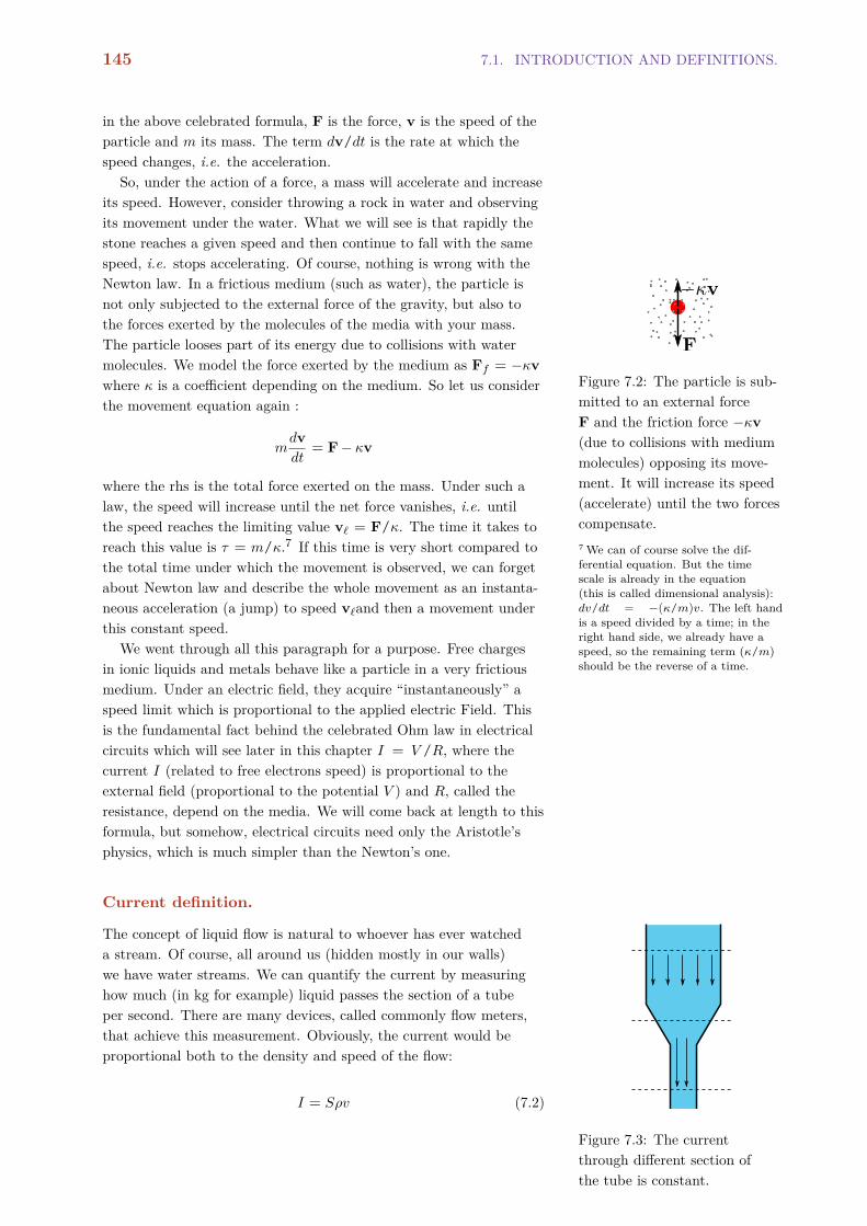
145 7.1. INTRODUCTION AND DEFINITIONS.
in the above celebrated formula, F is the force, v is the speed of theparticle and m its mass. The term dv/dt is the rate at which thespeed changes, i.e. the acceleration.
So, under the action of a force, a mass will accelerate and increaseits speed. However, consider throwing a rock in water and observingits movement under the water. What we will see is that rapidly thestone reaches a given speed and then continue to fall with the samespeed, i.e. stops accelerating. Of course, nothing is wrong with theNewton law. In a frictious medium (such as water), the particle isnot only subjected to the external force of the gravity, but also tothe forces exerted by the molecules of the media with your mass.The particle looses part of its energy due to collisions with watermolecules. We model the force exerted by the medium as Ff = −κvwhere κ is a coefficient depending on the medium. So let us considerthe movement equation again :
Figure 7.2: The particle is sub-mitted to an external forceF and the friction force −κv(due to collisions with mediummolecules) opposing its move-ment. It will increase its speed(accelerate) until the two forcescompensate.
mdvdt
= F− κv
where the rhs is the total force exerted on the mass. Under such alaw, the speed will increase until the net force vanishes, i.e. untilthe speed reaches the limiting value v` = F/κ. The time it takes toreach this value is τ = m/κ.7 If this time is very short compared to 7 We can of course solve the dif-
ferential equation. But the timescale is already in the equation(this is called dimensional analysis):dv/dt = −(κ/m)v. The left handis a speed divided by a time; in theright hand side, we already have aspeed, so the remaining term (κ/m)should be the reverse of a time.
the total time under which the movement is observed, we can forgetabout Newton law and describe the whole movement as an instanta-neous acceleration (a jump) to speed v`and then a movement underthis constant speed.
We went through all this paragraph for a purpose. Free chargesin ionic liquids and metals behave like a particle in a very frictiousmedium. Under an electric field, they acquire “instantaneously” aspeed limit which is proportional to the applied electric Field. Thisis the fundamental fact behind the celebrated Ohm law in electricalcircuits which will see later in this chapter I = V /R, where thecurrent I (related to free electrons speed) is proportional to theexternal field (proportional to the potential V ) and R, called theresistance, depend on the media. We will come back at length to thisformula, but somehow, electrical circuits need only the Aristotle’sphysics, which is much simpler than the Newton’s one.
Current definition.
The concept of liquid flow is natural to whoever has ever watcheda stream. Of course, all around us (hidden mostly in our walls)we have water streams. We can quantify the current by measuringhow much (in kg for example) liquid passes the section of a tubeper second. There are many devices, called commonly flow meters,that achieve this measurement. Obviously, the current would beproportional both to the density and speed of the flow:
Figure 7.3: The currentthrough different section ofthe tube is constant.
I = Sρv (7.2)

CHAPTER 7. ELECTRICAL CIRCUITS. 146
where S is the cross section of the tube, ρ the liquid density (inkg/m3) and v its speed ( in m/s).
Consider a tube which has a varying diameter along its length,and consider two cross section of this tube. For an incompressibleflow, whatever crosses the first section would have to cross the sec-ond section during the same amount of time: by definition of incom-pressible flow, the liquid cannot change its density and accumulate insome part of the tube. Physically, the fluid achieves the invariance ofthe flow by changing its speed.
The above discussion can be repeated for the electric current. Theelectric current I is the amount of charges which crosses a section ofthe circuit per unit of time. Equation (7.2) remains valid if we takethe definition of ρ to be the charge density (in C/m3). The currentis so much used that it has received its own unit, which is calledthe Ampere (A). One Coulomb per second crossing a section of thecircuit is one Ampere.
The electron fluid is incompressible : throughout the wire, thecurrent is constant.
Sources of current generation.
+
Figure 7.4: Each time an elec-tron leaves one end of the wire,another is injected into thewire, from the other end by thebattery. The chemical interac-tion inside the battery insurethat the electron inside the bat-tery is transported from the +pole to the - one.
Let us consider a copper wire which we connect to an electric fieldsource such as a battery. The free electrons will move under the fieldand get out of the wire. But this cannot last : when a very smallfraction of electrons have left the wire, the net charge of the wire willbecome positive and strongly attract the remaining electrons8, which
8 Did I mention that opposingcharges attracts each other ? Iguessed that the reader is aware ofthis well known fact, studied firstquantitatively by Coulomb around1790.
cannot leave anymore and all movements will stop.So this is not the whole story. In fact, for each electrons which
leaves the wire at on end, the battery injects an electron at the otherend, so the net charge inside the wire always stays at zero! Thebattery itself uses the energy extracted from chemical reactions toachieve this feat (Figure 7.4). We will learn more about the batteryin the chapter dedicated to thermodynamics. For the moment it isenough for us to think of the battery as dual role of providing anelectric field to move the charges and compensating for charges.
We will use throughout this chapter the analogy between electriccurrent and incompressible liquid flow in tubings. Let us state thatin this analogy, the analog of the power source in electricity is thehydraulic pump. We don’t need to know its inner working, suffice tosay that it provides the energy to move the fluid.
There are many ways to make an electric power source for mov-ing charges. The chemical battery we mentioned above was firstmade by Volta around 1800. The batteries at this time were not verystable and for his experiments, Ohm used a source based on ther-moelectric effects : connect one end of two rods made from differentmetal and heat them ; the two other non connected end will be theplus and minus end of your battery. Nowadays, the direct current weare speaking about is mostly furnished by electronic devices (calledpower supplies) plugged into the AC current available everywhere.

147 7.1. INTRODUCTION AND DEFINITIONS.
We will come to various kind of currents below.
7.1.1 Measuring the electric current.
Whatever we say about electric current and electricity in generalwould not have been possible if we didn’t have a device to measurethe electric current. There is a very intimate relationship betweenelectricity and magnetism9. Oersted discovered in 1820 that an 9 There are in fact the same thing.
As humans, we separate time fromspace. It was discovered in 1905 byEinstein that time and space arethe same thing. Distinction betweenElectric and Magnetic field orig-inated because of the distinctionbetween time and space and wereunified thereafter. They are the vari-ous component of the derivative of a4 dimensional vector.
electric current can deflect the magnetic needle of a compass. Verysoon, the amplitude of needle’s deflection led to an apparatus calleda Galvanometer, (even though Galvani, a scientist from an earliergeneration, had no contribution to this invention) to measure theelectric current in a precise quantitative way. One could still seeGalvanometers in the laboratory some thirty years ago (when theauthor of these lines was a student), and their use needed some care.Nowadays they are replaced with digital ammeters that don’t needanymore the careful observation of the needle.
7.1.2 AC/DC.
As the reader suspects, we don’t speak about music here, but aboutDirect current (DC) versus Alternative current (AC).
Figure 7.5: Rotation of a pointaround a center, modeled by acomplex number z.
The two most simple type of movement we observe in nature aretranslation with constant speed and rotation with constant speed.For rotation, the term speed v is replaced by angular frequency ω.The unit of angular frequency is radian/s; as radian is just a plainnumber, the unit of ω is s−1.
Consider a wheel rotating at constant ω, and a point P on thewheel (Fig. 7.5). We can use a complex number z to follow the pointP , in which case the position of P relative to the wheel center iswritten
z(t) = rei(ωt+φ)
where r is the wheel radius. At time t = 0, the position of P isz(0) = reiφ, the term φ is called the phase of the point. At latertimes t > 0, the position is given by z(t) = z(0)eiωt. Complexnumber are very useful to follow plane rotation10. Of course, if we 10 The relation between complex
numbers and rotation is due toEuler, back in the ~1740
need to characterize the point P by its projections on x and y axis,we only need to consider the real and imaginary part of z(t) :
x(t) = r cos(ωt+ φ) ; y(t) = r sin(ωt+ φ) (7.3)
The movement of the projection of the point P on an axis is calledan alternating movement, with angular frequency ω and phase φinherited from the rotating wheel. Any alternating signal of theform (7.3) can be seen as the projection of a rotation modeled by acomplex number.
The reason rotations are so used by humans is that rotation andtranslation can easily transform into each other : the rotation ofthe wheel is transformed into a linear motion of the car11. On the 11 The wheel is one of the greatest
achievements of humans, on thesame level as the discovery of fire.One theory relates the spread ofindo-europeans to their control ofwheeled movements. See “The Horse,the Wheel, and Language” by D.W.Anthony.
other hand, the linear movement of the stream’s fluid in converted torotation in a watermill.

CHAPTER 7. ELECTRICAL CIRCUITS. 148
By the end of XIX-th century, scientists and engineer realizedthat this is in fact an extremely powerful way of generating current12 12 The phenomenon was studied
first by Ampère and Faraday in the1820-40.
V
Figure 7.6: The simplest Al-ternator, turning a permanentmagnet inside a wire loop.Source : Wikipedia/Egmond.
: just rotate a permanent magnet around electrical wire and voilà: you have an alternating electric current in the wires (Fig. 7.6).In-side the wire, the electron fluid performs an alternating movement asa whole (Fig. 7.7), and is of the form
I(t) = I0 cos(ωt+ φ)
and we will model this current by the complex number
I = I0eiφ
For all practical uses we will make of the electric current in thefollowing sections, there is no important differences between AC andDC.
Figure 7.7: In AC, The electronfluid (blue) performs an alter-nating movement as a wholeinside the wire (brown).

149 7.2. THE OHM’S LAW.
7.2 The Ohm’s law.
7.2.1 Hydraulic analogy.
In order to understand the Ohm’s law, which is the fundamentalrelation of electricity, it is worthwhile to push forward with thehydraulic analogy.
Figure 7.8: A Reservoir (R)placed at a height h is con-nected to a Ground station (G)through a tube (T). A pump(P) keeps the reservoir filledand closes the circuit.
Consider a reservoir placed at a height h which is connectedthrough a tube to a ground station (7.8). Due to pressure difference∆P between the (bottom of the) reservoir and the ground, waterflows in the tube. The reservoir itself is kept filled by a pump.
The water flowing in the tube looses part of its kinetic energyas heat. We can therefore characterize the tube by its resistanceto flow, which captures this energy loss and which depends on thetube’s geometry (cross section, length, bends, ...).
What we are thought in a hydraulic lecture is that the current inthe tube is proportional to the pressure difference ∆P :
I = ∆P/R (7.4)
where R is the tube resistance we spoke about. In fact, this is usedas the definition of the resistance. The above equation is an exper-imental fact and its beauty resides in the fact that the current andthe pressure are proportional.
In many hydraulic circuits, the reservoir is omitted and the pres-sure pump alone make the water flow through various tubing. Thereare various kind of pumps possessing feedback control elements inorder to keep a constant pressure difference regardless of the current.In the following, we will consider the pump just as an ideal source ofmaking pressure difference in the circuit.
Figure 7.9: A hydraulic circuitwith a pump (pressure source)and various tubings.
Now, consider the circuit of figure 7.9. The pump furnishes apressure difference ∆Poi = Po − Pi. There are many tubings andwe’ll suppose that we know each pipe’s resistance. We can of coursemeasure the pressure difference in each part ∆Pij = Pi − Pj andverify relation (7.4) in this part I = ∆Pij/Rij . The instrument tomeasure pressure is called a manometer (or a pressure gauge). Twoobvious facts deserves to be stressed:
1. The total pressure difference ∆Poi equals the sum of pressuredrops in each section:
∆P =∑i
∆Pij
where we have omitted the subscript oi for the pressure source.
2. The fluid is incompressible, so the current is the same in all pipes.
The relation (7.4) between pressure and current is so good thatif we know before hand the resistance of each tube (Rij), we candetermine the pressure at each point by measuring only the current:
∆Pij = RijI

CHAPTER 7. ELECTRICAL CIRCUITS. 150
7.2.2 Electric circuits.
An electric circuit is a close analog of a hydraulic circuit. The in-compressible electron fluid flows through various wires with theirelectric resistance. The unit of electric resistance is called the Ohm.The source of the flow is an instrument which establishes a Voltagedifference in the circuit, usually a battery or a power supply. Theunit of Voltage difference is appropriately called the Volt.
+-
Figure 7.10: An electric circuitis formed of a power supplywhich provides a potentialdifference ∆V = V+ − V−.The electric current I flowsthrough various wires of thecircuits, with resistance Ri. AVoltmeter can measure the po-tential difference ∆Vij betweentwo points of the circuit.
The instrument which measures the potential difference is calleda Voltmeter. The Voltmeter has two electrodes; when the electrodesare positioned at two different part of the circuit, the voltmeterpanel indicates the potential difference between these two pointsof the circuit. It is important to note that we have no instrumentwhich can measure absolute potentials, but only difference of poten-tials, or relative potentials13. Because of that, it is customary to set
13 Nothing special about electric-ity here. The electric potential isrelated to the concept of potentialenergy, which itself is defined up to aconstant.
(arbitrary) one point of the circuit at potential V = 0, and mea-sure potentials at various points relative to this point. This point iscalled the ground and usually it is chosen to be the minus pole of thepower supply.
The Ohm’s law is the analog of the relation (7.4):
I = ∆V /R (7.5)
where R is the electric resistance of the part of the circuit underconsideration, and ∆V the potential difference between the bordersof the resistor. Usually, we are too lazy to write ∆V , so the relationis more often than not is written I = V /R.
Figure 7.11: Resistors used incircuits come in many formsuch as this one. The ac-tual value of its resistanceis coded into colors. ImageSource:Wikipedia
The Ohm’s law can be used in many ways. In relation (7.5), weknow V and R and we determine I. But of course, if we know twoelements, we know the third. So for example,
V = RI
is used when we know R and I and we want to measure V . Notethat if R = 0, V = 0 : there is no potential drop over a non-resistiveelement.Usually, the resistance of a good copper wire is very (veryvery small) compared to resistive elements inserted in a circuit (suchas a light bulb or a computer). In general, we will approximate thewire resistance to 0. Usually, the resistance of a good copper wireis very (very very small) compared to resistive elements inserted ina circuit (such as a light bulb or a computer). In general, we willapproximate the wire resistance to 0. This make the scheme of acircuit easier to draw : all points connected to the ground point by awire are sketched by a terminal symbols.
+-
+-
Figure 7.12: Simplifying electri-cal sketches: points connectedto the ground by a resistance-less wire are terminated withthe ground symbol.
Finally, if we want to measure the resistance of an element bymeasuring the potential and the current, we will use
R = V /I
7.2.3 Series and parallel resistors.
Consider two resistors in series. What is the current I in this circuitelement if we know VA and VC? Writing the Ohm’s law for the two

151 7.2. THE OHM’S LAW.
resistors, we have
Figure 7.13: Resistors in seriescan be replaced by an equiva-lent resistor Re = R1 +R2 + ...
VA − VB = R1I
VB − VC = R2I
We have two unknowns (VB and I ) and two equations, so the abovelinear system is well defined. On the other hand, we only asked forI and the value of VB is of no consequence to us. Summing the twoequations, we have
VA − VC = (R1 +R2)I
the term VA − VC = V is the potential difference across the tworesistors taken together. So we have
I = V /Re
where Re = R1 +R2.Re is the equivalent resistance of the two elements placed in the
circuit. In general, we can simplify an electric sketch each time wesee n resistors in series by the equivalence relation
Re =n∑i=1
Ri
Note that resistors together in series have increased resistance com-pared to each individual resistance: Re > Ri.
Consider now two resistors in parallel. The incoming current Iis divided into I1 and I2, flowing through resistors R1 and R2 andjoining again at point B. What is the potential drop V = VA − VB ifwe know the incoming current I and the two resistance R1 and R2?
Figure 7.14: Equivalent parallelcircuit
Let us write the Ohm’s law for the element of the circuit :
V = R1I1
V = R2I2
In this linear system, we have three unknown (V ,I1,I2) and twoknown (R1,R2). We also know that the current is incompressible andtherefore
I1 + I2 = I
So the Ohm’s law and the current conservation law give us exactlyenough equation to find our unknowns. We did not ask for I1 and I2.The third relation can thus be written as
I = V
(1R1
+1R2
)(7.6) 0.0 0.2 0.4 0.6 0.8 1.00
2
4
6
8
10
R1R2Re
1R1
1R2
1R1+ 1R2
Figure 7.15: Graphical deter-mination of parallel equivalentresistance Re. (i) locate R1 andR2 on the horizontal axis, andfind the corresponding 1/R1and 1/R2 on the vertical axisusing the 1/x graph (red ar-rows). (ii) perform the sum1/R1 + 1/R2 on the verticalaxis and find Re on the hor-izontal axis using the graph(cyan arrows)
and therefore the potential drop V is simple V = ReI where theequivalent resistance is given by the term inside the parenthesis. Forn resistors in parallel, the equivalent resistance is Re, where
1Re
=n∑i=1
1Ri
(7.7)

CHAPTER 7. ELECTRICAL CIRCUITS. 152
equation (7.7) can be understood graphically (figure 7.15). It is thenobvious that for parallel resistance, Re < Ri, i.e. the resistance ofthe ensemble is reduced compared to each resistance.
Note that relation (7.7) is a particular case of an f−sum. Thef−sum generalizes the usual sum; given a function f(x), the f−sumof variables x1, ...,xn is defined as xe, where
f(xe) =n∑i=1
f(xi)
the f−sums appears in many area of physics (such as in thermody-namics, where they define the free energy). It is fruitful to think off−sums in graphical terms (figure 7.15).
7.2.4 Note on the Voltmeter.
Did we see above how a voltmeter works ? No, we did not. Thereason for this omission is very simple : there is no such instrumentavailable. All the voltmeters are indeed ammeters possessing a veryhigh resistance Ra , mounted in parallel with the section we aremeasuring. A small portion of the current is derived into this circuit(this is the reason for the high entry resistance) and the measuredcurrent is converted to potential through the Ohm’s law. Whendoing very accurate measurements, we have to take into account thissmall perturbation to the circuit.
We could build a Voltmeter in the absence of electric current, forexample connecting two metallic plates to the two sides of a batteryand measuring the forces between them and use this forces as aproxy for calibrating the potential. Indeed, the very definition of aVolt depends on such concepts. But measuring currents is so preciseand robust that there is no need for a “true” voltmeter. Moderndigital voltmeter (based on electronic circuits, and having their owninternal power supply) have such a high input resistance (GΩ) thatwe can forget about perturbation to the circuit.
Note on the Ohm’s law.
Ohm himself did not measure independently current and potential,so how did he came to formulate his law ? When Ohm began work-ing (~1825) on this problem, the concept of potential and resistancewere unknown. There was no reliable power source and the Voltabattery was far from perfection. To have a reliable power source,Ohm used an thermoelectric battery, which doesn’t provide muchpower but is much more stable in time than the electrochemicalVolta battery was at this time(figure 7.16) .
Figure 7.16: Thermoelectricbattery. The voltage providedby this battery depends on thetemperature gradient and thetype of metal used.
Ohm used various battery (different heating, different metals) andvarious wires (different metals, different length and cross section)and for each combination, he measured the current I by a (thenstandard) galvanometer. He noticed that all his measurements canbe put in the form of
I =AS
BS +CW(7.8)

153 7.2. THE OHM’S LAW.
the term AS and BS depended only on the power source used, whilethe term CW depended only on the type of wire. More over, the CWterm could be written as
Cw = ρLength
Cross section (7.9)
where the parameter ρ depended only on the type of the material.He called the numerator the electromotive force of the power source.Nowadays, we would write this relation as
+-
Figure 7.17: A real powersource V (red circle) has al-ways an internal resistance rwhich is considered as in serieswith the circuit.
I =V
r+R
where V is the potential, r is the intrinsic resistance of the powersource and R is the resistance of the wire. Usually, in all circuits wemake, r R so we neglect this term and write the relation simply asI = V /R. However, this approximation breaks down if R ≈ 0 : evenwith zero resistance, the power source can only provide a limitedquantity of current. We consider the intrinsic resistance of the powersource to be in series with the circuits resistance (figure 7.17).
The ρ term in equation (7.9) is called the resistivity and dependsonly on the material used. It is very low for usual metals (calledtherefore conductors) and is very high for ceramics (called insula-tors). Materials having the intermediate resistivity are called semi-conductors; they are used as control elements in electric circuitsthough devices called diodes, transistors, ...
7.2.5 Note on linear equations.
Any complicated circuit made of linear elements (resistors, capaci-tors, inductors) can be translated into a linear system of equationssuch as the ones we studied above. So any circuit can be solved bythe general methods of linear systems we studied previously in thechapter dedicated to mathematics.
The particularity of the electric systems is that in general, theirmatrix is sparse and contains many zero. The sketch of the circuit isa big help in solving these equations : for example, series and paral-lel resistance can be grouped together. People have developed manytricks on the efficient solution of electrical circuits and their tricksare called “theorem” in electrical engineering (Thevenin, Norton, ...).A very nice trick is called “mesh currents” methods which in mathe-matical term, removes most of the useless zero from the matrix andreduces the matrix to lower dimensionality (and mostly diagonal).
As usual, the best way to get used to solving electrical circuitsand these tricks is to solve problems.
7.2.6 General Principles to solve circuits.
Circuits can get complicated with many branches in serial and par-allel. Keeping in mind few general principles will greatly simply thecircuit.
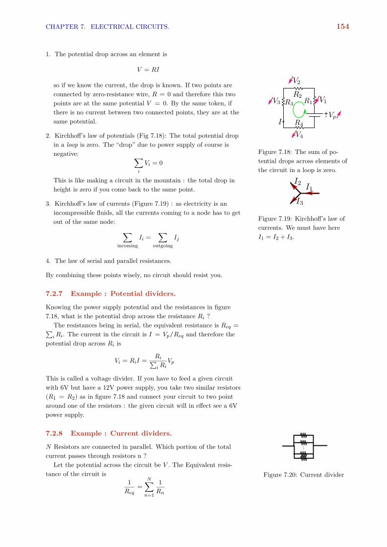
CHAPTER 7. ELECTRICAL CIRCUITS. 154
1. The potential drop across an element is
V = RI
so if we know the current, the drop is known. If two points areconnected by zero-resistance wire, R = 0 and therefore this twopoints are at the same potential V = 0. By the same token, ifthere is no current between two connected points, they are at thesame potential.
+-
Figure 7.18: The sum of po-tential drops across elements ofthe circuit in a loop is zero.
2. Kirchhoff’s law of potentials (Fig 7.18): The total potential dropin a loop is zero. The “drop” due to power supply of course isnegative: ∑
i
Vi = 0
This is like making a circuit in the mountain : the total drop inheight is zero if you come back to the same point.
Figure 7.19: Kirchhoff’s law ofcurrents. We must have hereI1 = I2 + I3.
3. Kirchhoff’s law of currents (Figure 7.19) : as electricity is anincompressible fluids, all the currents coming to a node has to getout of the same node: ∑
incomingIi =
∑outgoing
Ij
4. The law of serial and parallel resistances.
By combining these points wisely, no circuit should resist you.
7.2.7 Example : Potential dividers.
Knowing the power supply potential and the resistances in figure7.18, what is the potential drop across the resistance Ri ?
The resistances being in serial, the equivalent resistance is Req =∑iRi. The current in the circuit is I = Vp/Req and therefore the
potential drop across Ri is
Vi = RiI =Ri∑iRi
Vp
This is called a voltage divider. If you have to feed a given circuitwith 6V but have a 12V power supply, you take two similar resistors(R1 = R2) as in figure 7.18 and connect your circuit to two pointaround one of the resistors : the given circuit will in effect see a 6Vpower supply.
7.2.8 Example : Current dividers.
N Resistors are connected in parallel. Which portion of the totalcurrent passes through resistors n ?
Figure 7.20: Current dividerLet the potential across the circuit be V . The Equivalent resis-
tance of the circuit is1Req
=N∑n=1
1Rn

155 7.2. THE OHM’S LAW.
and the total currentI =
V
Req
The current through resistor n is In = V /Rn therefore
InI
=ReqRn
Note that if Rn → 0 (is very small compared to other resistors),Req ≈ Rn and therefore In ≈ I : all the current pass through thisresistor.
7.2.9 Example : the Wheatstone bridge.
This is a very fine method to measure an unknown resistance by us-ing three known resistors, one of which is a variable resistance(figure??). There is no need to know/measure the power supply voltage(which can have low precision) or the current out of it.
Figure 7.21: The Wheatstonebridge.
Consider the above circuit (figure 7.21), where Rx is the unknownresistance and R2 the variable one, while R1 and R3 are fixed. Thiscircuit has 8 unknowns (the 6 currents and VB , VC) and 8 equations(4 potential-current relation and 4 current conservation).
In practical terms however, the task is much easier. We varythe resistance R2 until there is no current in the BC branch. Thepresence or absence of current is measured by an ammeter insertedin the BC branch. When this happen, We know that
I1 = (VA − VB)/R2 = (VB − VD)/R1 (7.10)I2 = (VA − VC)/Rx = (VC − VD)/R3 (7.11)
We can write the first line for example because there is no current inBC, hence all the current through R2 has to pass through R1. Moreover, As
VBC = VB − VC = RBCIBC = 0
we must have VB = VC . Using this and dividing the two lines ofequations (7.10,7.11), we obtain
RxR2
=R3R1
or Rx = (R2/R1)R3.The term R2/R1 acts as a lever, allowing to find very low or
very high resistances. The difference method, detecting a non-zerocurrent, is a very sensitive method.
What we saw in the above example is a practical solution whichgoes directly to the solution, without solving for uncalled for vari-ables.

CHAPTER 7. ELECTRICAL CIRCUITS. 156
7.3 Energy and power.
For the moment, we have discussed electricity without discussing theconcept of energy and power. The sources we have in our circuitshave however a limited amount of stored energy (chemical potentialenergy) and this limitation can become important in our computa-tions if we are drawing to much power .
How much energy does a circuit dissipate across a resistance R ?As you remember, the speed of the charges, and hence the currentI is proportional to potential variation across the circuit. As wesaw in the definition of power (eq. 6.30), the power is a force (here∝ V ) multiplied by a speed (here ∝ I) and so we should have P ∝V I. In fact, if we go into more details about how the potential V isdefined from electromagnetism theory and what is the work done ona charge, we would see that the relation is exact and very general i.e.not restricted to resistive elements :
P = V I (7.12)
The unit of power is W as usual, and sometimes the equivalent VA(Volt-Ampere) is used
For a resistive element connected to power source, using the Ohmlaw, we have
PR =V 2
R= RI2
this is the amount of energy dissipated into the environment perunit of time. It causes heating. A major limitations of computer isthe amount of heat they can effectively dissipate instead of gettingmelted by this Joule effect.
§ 7.1 The Edison light bulb we were used to have at home converted must ofthe injected energy into heat, and very little into light. How long do we haveto switch on a 100W bulb in order to make 1L of water to boil ?
Solution. Supposing that the heat capacity of water in constant betweenroom temperature 20C and the boiling point 100C and equal to 4200J/kg.C,we see that we need a total heat (energy) of E = 80× 4200 = 3.76× 10⁵J,and therefore we need t = 3.76× 10³s ≈ 1hr of our light bulb.
A normal battery however can store only a limited amount ofEnergy. Unfortunately, the unit of this energy is not given in J butin Wh (Watt-Hour, 1Wh=3.6kJ). Even worse, when a battery issupposed to provide a constant potential V over time, the energystored is given as something like 2500mAh 1.2V which means thatthe battery can provide a current of 2.5A for 1 hour with a nominalpotential of 1.2V (i.e. ≈ 10kJ).
Now, suppose that we plug a small resistance, say 1mΩ into a(nominal) 6V battery with 10kJ capacity. The power drained fromthe battery is 3.6× 10⁴W, so in a fraction of seconds the battery isdrained ; during this time, the current provided by this battery is6kA ! Something is very wrong in our computation.
The error is to think that the battery will maintain a nominalpotential of 6V (or that such a current could be delivered) whatever

157 7.4. THE AC REVISITED.
resistance is plugged into. From the first experiment of Ohm in 1830it was realized that the relation I = V /R is just an approximationwhich breaks down for small R. As we saw (eq.7.8 and the accompa-nying note) The exact relation derived by Ohm was
I =V
R+ re
where both V and re depend on the power source and R on theexternal resistance. The quantity re is called the internal resistanceof power source. We see that even if we make a short circuit withR = 0, the battery can at best deliver a current of I = V /re and apower of V 2/re. For example, an 1.5V AA battery has re ≈ 1Ω anddelivers at most P = 2.25W (figure 7.22
10-2 10-1 100 101 102 103
R
10-3
10-2
10-1
100
101
102
103
I
real
ideal
Figure 7.22: Current deliveredby a real 1.5V battery withinternal resistance re = 1Ω,as a function of the pluggedresistance R. For R re, thebehavior is close to the idealbehavior ; for R re however,the current delivered saturatesand is far from the ideal model.
7.4 The AC revisited.
As we mentioned at the beginning of this chapter, AC currents arewidely used around us; AC is the major type of current producedby humans and most of DC current used in our electronic devices isderived from AC sources.
Working with AC also allows for the use of new types of elementswhich do not exist in DC. These are mainly the capacitor and theinductor. These new elements enable us to do a whole new kind ofwork, such as detecting a radio wave at a particular frequency anddemodulate it.
7.4.1 AC Take Home message.
Before developing the theory below, let us stress the important pointto understand. When a linear circuit having resistors, capacitors andinductors (to be defined below) is submitted to a sinusoidal powersource V (t) = V0 cos(ωt), every elements of the circuit ( variouscurrents and potential drops) will display the same oscillation, witha phase shift. If the quantity we are measuring is S(t), then we willhave
S(t) = S0 cos(ωt+ φ)
A great simplification occurs when we group the amplitude S0 andthe shift φ into a single complex variable S = S0 exp(jφ) wherej2 = −1 is the unit imaginary number. First of all, the signal S(t)can simply be written as S(t) = Re[S exp(jωt)]. But more im-portantly, everything we saw about DC circuits (serial and parallelresistance, current conservation, potential drops in a loop, ...) con-tinues to apply to these complex variables. For that, we only haveto generalize the resistance to complex resistance, which we wouldcall impedance. For example, for a pure resistance, ZR = R, butfor a capacitor, ZC = 1/jCω and for an inductor, ZL = jLω. Thepotential drop across an impedance Z (which can be a combinationof R, L and C elements in serial and parallel) will be V = ZI.
Going to the complex domain allows us to use the same simplemethodology as in DC. Once we have computed a complex signal S,

CHAPTER 7. ELECTRICAL CIRCUITS. 158
we know that its time dependence is S(t) = S0 cos(ωt+ φ) whereS0 = |S| and φ = Arg(S).
7.4.2 New element : capacitors.
A capacitor is a device to store a small amount of charges. It’s madeof two metallic plates separated by an isolator (figure 7.23). Whenconnected to a potential difference V , charges of ±Q accumulate onits plates. The amount of charge accumulated per applied voltage iscalled the capacity C +
-
+++++++++
-----------
Figure 7.23: Capacitor.
C =Q
V(7.13)
the unit of capacity is the Farad (F). You wouldn’t be able to buy aFarad in the electronic shop near you, the best you could do wouldbe to buy nano to micro farads.
As we mentioned many times, the electron fluid is an incompress-ible flow. However, the capacitor plays the role of a store room, areservoir capable of storing a small amount of charge. Consider thefigure 7.23 circuit, where the power supply is switched on and thepotential V (t) goes from zero to some value in time. We know fromthe relation above that
V (t) =1CQ(t) (7.14)
where Q(t) is the charge in the condenser at time t. Charges ac-cumulate on the plate because electric current is flowing from thebattery. During a short interval dt, the amount of charge comingto the condenser is dQ = Idt, where I is the current in the circuit.Deriving relation (7.14) we therefore have
dV
dt=
1CI (7.15)
There are few cases worth considering.(i) Suppose first that the potential goes from zero to Vmax on a τ
timescale : V (t) = Vmax(1− exp(−t/τ )). In this case, the current inthe circuit would be
0 1 2 3 4 5 6
t0.0
0.2
0.4
0.6
0.8
1.0
V(t)
I(t)
Figure 7.24: I(t) and V (t) fora capacitor, when V increasesto a saturation value.
I(t) =C
τVmaxe
−t/τ (7.16)
which means that the current goes from a high value CVmax/τ tozero : after a time τ , there is no more current. In other words, acapacitor cannot work in a DC current except for a short time. Thesecond fact worth noticing is that, comparing to the Ohm’s law forresistors, τ/C has the dimension of a resistance : [C/τ ] = [1/R] sowe know that we can define 1 Farad by 1 sΩ−1.
(ii) Consider now an alternative power supply, i.e. V (t) =
V0 cos(ωt) then from relation (7.15) we have0 5 10 15 20
t
−1.0
−0.5
0.0
0.5
1.0
V(t)
I(t)
Figure 7.25: I(t) and V (t) fora capacitor, when V oscillates.
I(t) = −V0(Cω) sin(ωt)
We see (figure 7.25) here that as long as V oscillates, I does thesame. You have surely noticed that there is a lag between the twoquantities.
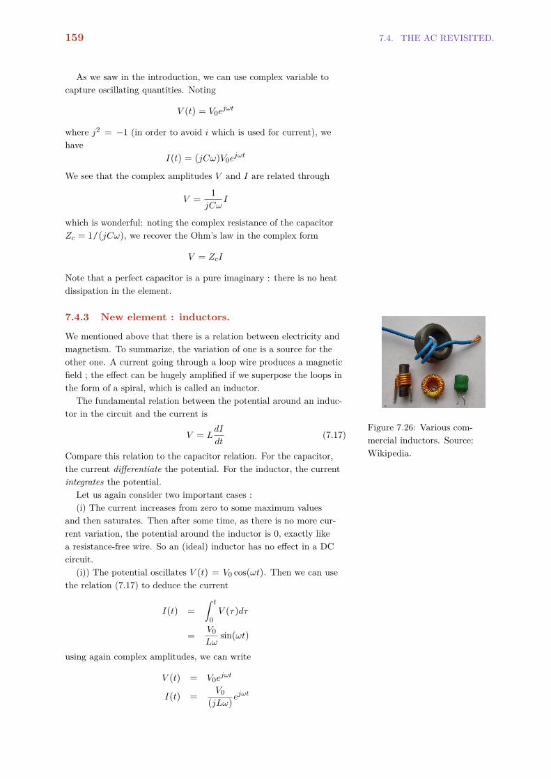
159 7.4. THE AC REVISITED.
As we saw in the introduction, we can use complex variable tocapture oscillating quantities. Noting
V (t) = V0ejωt
where j2 = −1 (in order to avoid i which is used for current), wehave
I(t) = (jCω)V0ejωt
We see that the complex amplitudes V and I are related through
V =1
jCωI
which is wonderful: noting the complex resistance of the capacitorZc = 1/(jCω), we recover the Ohm’s law in the complex form
V = ZcI
Note that a perfect capacitor is a pure imaginary : there is no heatdissipation in the element.
7.4.3 New element : inductors.
We mentioned above that there is a relation between electricity andmagnetism. To summarize, the variation of one is a source for theother one. A current going through a loop wire produces a magneticfield ; the effect can be hugely amplified if we superpose the loops inthe form of a spiral, which is called an inductor.
Figure 7.26: Various com-mercial inductors. Source:Wikipedia.
The fundamental relation between the potential around an induc-tor in the circuit and the current is
V = LdI
dt(7.17)
Compare this relation to the capacitor relation. For the capacitor,the current differentiate the potential. For the inductor, the currentintegrates the potential.
Let us again consider two important cases :(i) The current increases from zero to some maximum values
and then saturates. Then after some time, as there is no more cur-rent variation, the potential around the inductor is 0, exactly likea resistance-free wire. So an (ideal) inductor has no effect in a DCcircuit.
(i)) The potential oscillates V (t) = V0 cos(ωt). Then we can usethe relation (7.17) to deduce the current
I(t) =
ˆ t
0V (τ )dτ
=V0Lω
sin(ωt)
using again complex amplitudes, we can write
V (t) = V0ejωt
I(t) =V0
(jLω)ejωt

CHAPTER 7. ELECTRICAL CIRCUITS. 160
and we recover again the Ohm’s law in complex form V = ZLI
where the impedance of the inductor is defined as
ZL = jLω
7.4.4 Fundamental equation of AC.
Consider the basic RLC circuit formed of an alternative powersource V (t) = V0 cos(ωt), a resistance R, a capacitor C and aninductor L. A current I(t) is flowing in the circuit. Calling VR, VL,VC the potential drop across the three elements, we have
Figure 7.27: The simplest RLCcircuit.
V = VR + VL + VC (7.18)
On the other hand, the current I(t) is the same in all part of thiscircuit (remember that the electron flow is incompressible). Aroundthe resistor, we must have VR = RI. Around the capacitor, we havedVC/dt = I/C and for the inductor VL = LdI/dt. So we can rewriteequation (7.18)
V = RI + LdI
dt+
1C
ˆ t
0I(τ )dτ (7.19)
Which is a second order differential equation in I, with a drivingterm V (t). We know how to solve these kind of equations. Once wehave determined I, we can determine potential drops across all theelements. Note that we can give equation (7.19) a better shape bydifferentiating it :
Ld2I
dt2+R
dI
dt+
1CI =
dV
dt(7.20)
When the driving force is sinusoidal, we know the solution beforehand: it should be of the form
I = I0 cos(ωt+ φ)
and here is when the complex notation comes in really handy. Writ-ing I = I0ejωt where I0 is the complex amplitude (taking intoaccount the phase exp(iφ), and replacing in (7.20), we have(
−Lω2 + jRω+1C
)I0 = jωV0
orI0 =
V0R+ (jLω+ 1/jCω)
Note that the denominator is
Z(ω) = R+ j(Lω− 1/Cω) (7.21)
and the impedance of the circuit depends on the oscillation fre-quency. The impedance is minimum (and the current maximum)when
ω = ωr = 1/√LC
ωr is called the natural or resonant frequency of the circuit.

161 7.4. THE AC REVISITED.
7.4.5 General principle of AC circuits.
The beauty of using complex variables is that AC circuits can besolved exactly as DC circuit : the law of serial and parallel resis-tances can be extended to any complex impedance, the ohm law onthe potential drop through a resistor V = RI is written know
V = ZI
the complex current is conserved is conserved at a node ...
7.4.6 Linear Filters.
Eliminating unwanted noise is part of the every day work we needto do to measure our signal. The general principle is to put a linearfilter between the incoming signal and the outgoing signal (figure7.28).
Figure 7.28: RLC (passive)filters.
The incoming signal Vin comes from your source : the radio an-tenna, the output of your PH meter, ... The outgoing signal goesto an amplifier before being send for further processing. We’ll dealwith the amplification process later in this chapter. What we needto know now is that the “out” circuit has generally a very highimpedance and draw very little current from the circuit; for all prac-tical purposes, we can neglect this current leak. What we are inter-ested in here is the inner circuitry of the linear filter which stronglydiminishes some unwanted frequencies.
The three widely used filters are band-pass, low-pass and highpass filters. Their most basic realization can all be obtained from theserial RLC circuit of figure 7.27, by measuring the potential acrossthe three elements.
Band-pass: The potential across the resistor is
VR = RI =R
ZV
and thereforeQ =
∣∣∣∣VoutVin
∣∣∣∣ = ∣∣∣∣RZ∣∣∣∣
where Z is given by relation (7.21). Note that when ω → 0 or ∞,Z → ∞ so the high and low frequencies are indeed reduced. Theexact form of Q is (figure 7.29)
Q(ω) =R√
R2 + (Lω− 1/Cω)2
and we see that for ω ω` = 1/(RC) we have Q(ω) ∼ RCω =
(ω/ω`) ; on the other hand, for ω ωh = R/L, we have Q(ω) ∼R/(Lω) = ωh/ω. ω` and ωh are the lower and higher cuttingfrequencies.
10-3 10-2 10-1 100 101 102 103
ω
10-2
10-1
100
Q
Figure 7.29: Band-Pass filtertransmission function. Reso-nant is marked by the verticalred dashed line. The blackdashed lines are ω and 1/ωfunctions.
Low-pass: If now we use the potential around the capacitor as theoutput signal, we have
10-3 10-2 10-1 100 101 102 103
ω
10-5
10-4
10-3
10-2
10-1
100
Q
Figure 7.30: Low-pass transmis-sion function. The dashed lineis the 1/ω2 function.

CHAPTER 7. ELECTRICAL CIRCUITS. 162
Q =
∣∣∣∣1/(Cω)Z
∣∣∣∣=
1/(Cω)√R2 + (Lω− 1/Cω)2
We see this time that if ω → 0, Q → 1 ; on the other hand, forhigh frequencies, ω → ∞, Q → 0. On the other hand, whenω = ω0 = 1/
√LC we have
Q =R∼R
where R∼ =√L/C. Depending on the relative value of R and
R∼, we may have a peak at ω = ω0. With this filter, only the lowfrequencies are transmitted.
High-pass: To transmit only the high frequencies, we use the poten-tial around the inductor. In this case,
10-3 10-2 10-1 100 101 102 103
ω
10-5
10-4
10-3
10-2
10-1
100
Q
Figure 7.31: Low-pass transmis-sion function.The dashed line isthe 1/ω2 function.
Q =
∣∣∣∣LωZ∣∣∣∣
=Lω√
R2 + (Lω− 1/Cω)2
We see this time that if ω → 0, Q → 0 ; on the other hand, forhigh frequencies, ω → ∞, Q → 0. As before, when ω = ω0 =
1/√LC we have Q = R∼/R where R∼ =
√L/C. Depending on
the relative value of R and R∼, we may have a peak at ω = ω0.Only the high frequencies are transmitted in this filter.
The filter we studied above are the crudest ones. Combining differ-ent elements can give mush more selective filters.
7.4.7 Exercise.
Study the transmission function of these filters.
7.4.8 Power dissipated by capacitor ans inductor.
A resistor dissipates energy in the form of heat. What about induc-tors and capacitors ? Consider a capacitor, where the current andpotential are related through
dV
dt=
1CI
Suppose an AC potential across this capacitor V = V0 cos(ωt) ; thecurrent through the capacitor is I = −CV0ω sin(ωt) and thereforethe power through this element is
P = −CV 20 sin(ωt) cos(ωt)
and the energy (work) of this element during one cycle T = 2π/ω is
W =
ˆ T
0P (t)dt = 0!

163 7.4. THE AC REVISITED.
A capacitor does not dissipate energy. It can stock and restore en-ergy, this is why P 6= 0 in general, but the balance over one cycleis zero and nothing is dissipated as heat. The same of course is trueof inductors. Of course, there is no ideal capacitor or inductor andthese elements always have also a (real) resistance, but the dissipa-tion is only due to the real resistance.
We can state that by using complex impedance for a generalelements, where V = ZI ; if Z if purely imaginary, we have P =
V 2/Z and therefore the power is also purely imaginary, which meansthat there is no dissipation. In general, energy dissipation is alwaysrelated to the real part of the impedance.
7.4.9 Advanced : PID controller.
7.4.10 Advanced : Lock-in amplifier.

CHAPTER 7. ELECTRICAL CIRCUITS. 164
7.5 Generalizing circuits.
Till now, we have pictured a circuit as a closed map where we can gofrom any point to any other point. This representation is too restric-tive and will forbid us to think of circuit as composed of modules,the behavior of each can be analyzed independently of others. Noone can design a complicated circuit with this kind a thinking. Fromnow on, we will think of elements as formed of electrical components,with an input and output part. In the literature, they are calledquadripoles or two-port networks (figure 7.32) . We have alreadyencountered them in the section on filtering .
Figure 7.32: (a) A generalquadripole ; (b) the Highpass filter represented as aquadripole.
The incoming signal can be from any source, a battery, the homeplug, the potential captured by the antenna of your radio. Thequadripole transforms the incoming signal into an outgoing signaland delivers it to another module. For example, the radio signalcaptured by the antenna is band-filtered and delivered to anothermodule to get amplified and to a final module made of the speakers.Any complex circuit is just the assembly of such modules and this iswhy indeed we can make them.
Until now, we had only used passive quadripoles in which theenergy is only dissipated. This wouldn’t get us far in the treatmentchain. Some modules contain internal power source in order to re-inject energy into the circuit and amplify the signal:
Vout(t) = AVin(t)
Amplification is among the most fundamental role in many electroniccircuit. Amplification must of course respect the integrity of thesignal, meaning that the gain A must be a constant in order not todeform the form of the incoming signal.
7.5.1 Diodes.
7.5.2 Transistors.
7.5.3 Op-amp.
Op-amp is negative feed-back component which is used in nearly anydesign. Negative feed back means that part of the output signal isre-injected back into the circuit and subtracted from the originalsignal in order to achieve a goal. We will see some of these goalsshortly.
VS+
VS
VoutV+
V
Figure 7.33: Op-Amp symbol.The op-amp power supply (Vs)is omitted in sketches.
The Op-amp is an active component, having its own power supplyand therefore can inject energy into the circuit. This external sourceis not shown in sketches ; however it should be taken into accountwhen looking at the limits of a given design.An op-amp has twoinputs differentiated by their sign and one output. The output mustalways be connected to the minus input through some connectorcapable of conducting a DC current. In order to compute the outputsignal for the ideal op-amp, there are only two rules:
1. The output potential is such that there is no voltage differencebetween the two inputs.
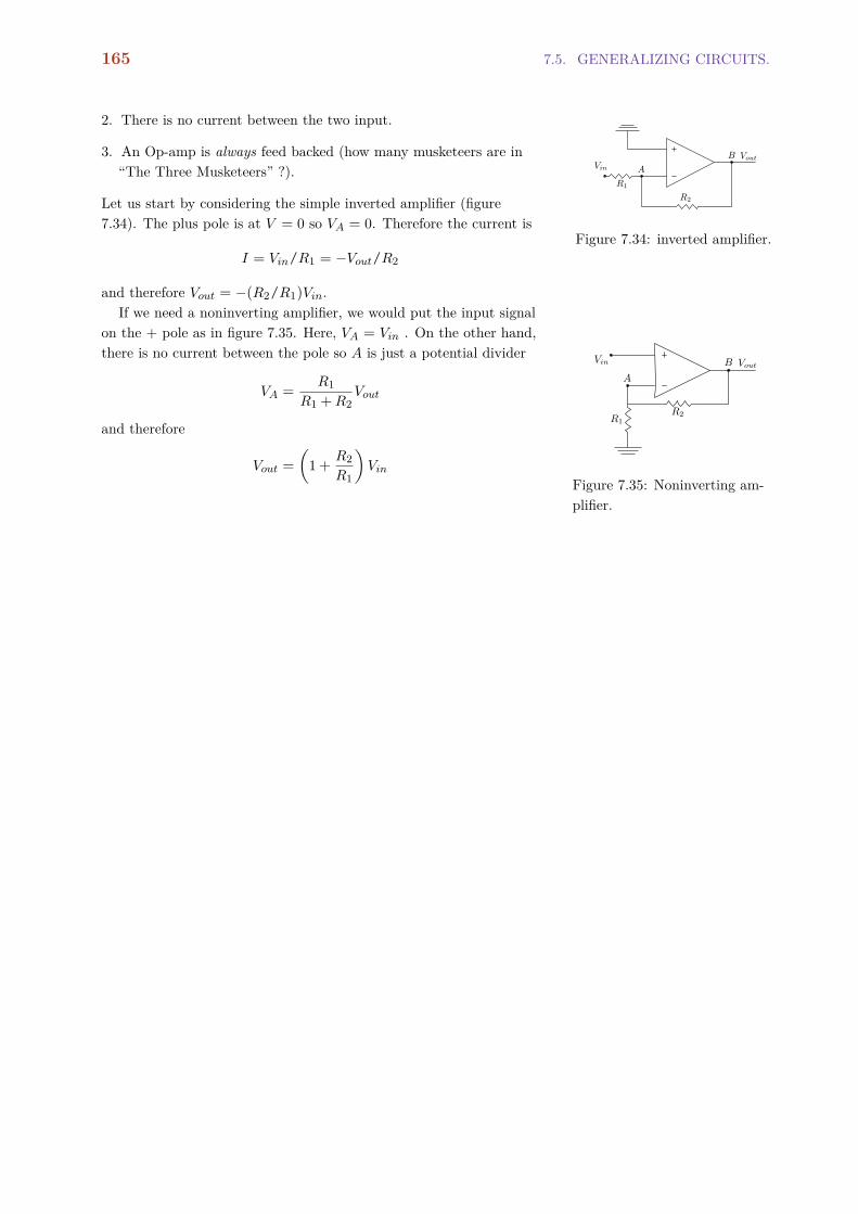
165 7.5. GENERALIZING CIRCUITS.
2. There is no current between the two input.
3. An Op-amp is always feed backed (how many musketeers are in“The Three Musketeers” ?).
Figure 7.34: inverted amplifier.
Let us start by considering the simple inverted amplifier (figure7.34). The plus pole is at V = 0 so VA = 0. Therefore the current is
I = Vin/R1 = −Vout/R2
and therefore Vout = −(R2/R1)Vin.If we need a noninverting amplifier, we would put the input signal
on the + pole as in figure 7.35. Here, VA = Vin . On the other hand,there is no current between the pole so A is just a potential divider
VA =R1
R1 +R2Vout
and therefore
Figure 7.35: Noninverting am-plifier.
Vout =
(1 + R2
R1
)Vin

CHAPTER 7. ELECTRICAL CIRCUITS. 166
7.6 Exercises.
Figure 7.36:
§ 7.2 Compute the current out of the power supply and the potential dropacross each resistor of figure 7.36. Try to use the concept of voltage divider.
Figure 7.37:
§ 7.3 Compute the current out of the power supply and in each branch andthe potential drop across each resistor of figure 7.37. Try to use the conceptof voltage and current divider.
Figure 7.38:
§ 7.4 A 6V power supply in connected to points A,B of figure 7.38. Computethe current out of it. All resistors are at 20Ω. What if we connect the powersupply to C,D ?
Figure 7.39:
§ 7.5 A 6V power supply in connected to points A,B of figure 7.39. Computethe current out of it. All resistors are at 20Ω.
Figure 7.40:
§ 7.6 Compute the impedance Z of the circuits of figure 7.40. Draw both|Z| as a function of ω, the angular frequency of the power supply. Computethe current through the two elements and discuss specifically the case forω = 0,∞,ω0 where ω0 = 1/
√LC.
Figure 7.41:
§ 7.7 Compute the impedance Z of the circuit of figure 7.41. Draw |Z| as afunction of ωthe angular frequency of the power supply. Compute the currentthrough the resistance R, and discuss specifically the case for ω = 0,∞,ω0where ω0 = 1/
√LC.
§ 7.8 Differential amplifierShow that for the circuit of figure 7.42, we have
Figure 7.42: Differential ampli-fier
Vout =R2R1
(V2 − V1)
§ 7.9 Additioning signalShow that for the circuit of figure 7.43, where all resistance are equals, we
have
Figure 7.43: Additionner
Vout = −(V2 + V1)
This is called an inverting summer.

Chapter 8
Thermodynamics.
Contents
8.1 The concept of energy. 169
8.2 Temperature. 170
8.3 Energy transfer. 171
8.4 Extensive and intensive parameters. 172
8.5 Heat capacity. 173
8.6 Work. 174
8.7 Equilibrium, reversible and irreversible changes. 176
8.8 Entropy. 177
8.9 Application to Perfect gases. 178
8.9.1 Internal energy. 179
8.9.2 Entropy. 180
8.9.3 Mathematical detour: constraints and differentials. 181
8.9.4 Heat capacity at constant pressure. 182
8.9.5 Adiabatic compression. 183
8.9.6 Joule expansion. 184
8.9.7 Perfect gas: conclusion. 185
8.10 The thermal machine: Carnot cycle. 185
8.11 The thermodynamic potential F and the minimum principle.189
8.11.1 The Helmholtz free energy. 189
8.11.2 The minimum principle. 190
8.11.3 Application to pressure. 191
8.11.4 Application to chemistry. 192
8.11.5 Application to surface tension. 193
8.12 Change of variables and generalized potentials. 193
8.12.1 The Legendre transform. 193
8.12.2 The Helmholtz free energy revisited. 195

CHAPTER 8. THERMODYNAMICS. 168
8.12.3 The Gibbs free energy. 196
8.12.4 Experimental determination of G. 196
8.13 The Maxwell relations. 198
8.13.1 General Relation between Cp and Cv 199
8.13.2 Application to osmotic pressure. 200
8.13.3 Contact angle, shape of drops, wetting, adsorption, surfactants 200
8.14 Statistical Physics. 201
8.14.1 A bit of history. 201
8.14.2 The fundamental relation. 202
8.14.3 Entropy revisited. 203
8.14.4 The internal energy and heat. 205
8.14.5 The minimum principle, again. 205

169 8.1. THE CONCEPT OF ENERGY.
Around 1712, Newcomen invented the first thermal machine:through cycles of heating, evaporating and cooling of water in acylinder, water could be pumped out of the mines, allowing min-ers to go deeper and deeper to find coal. This invention radicallychanged the history of humanity, allowing it to go (much) beyondequilibrium with its environment and tap the incredible amount ofenergy stored in earth’s crust. Humans discovered that heat can betransformed into work. Development of thermal machines led to thefield of thermodynamics through the work of many scientists suchas Carnot, Joule, Clausius, ... Soon, scientists discovered that thefield is not restricted to thermal machines but encompasses nearly allsciences at finite temperature.
In this lecture, we are not concerned by thermal machines andwill restrict ourselves to some problem related to physical chemistry.Before applying anything to anything however, we need to developmany concepts which are at the heart of this field. Some of theseconcepts, specially the concept of energy, have been more rigorouslydefined in chapter 6. I give here however a summary of what isneeded, in a less mathematically oriented fashion. Also, the nameof some symbols has been changed compared to chapter 6 in orderto avoid confusion, for example between the kinetic energy and thetemperature.
8.1 The concept of energy.
Moving objects can do work. This was obvious from the very ancienttime where for example water mills were used for grinding grain intoflour, using indeed the moving water to rotate the wheels ; anotherexample is wind use for sailing boats, where the moving air is usedto push the boat.
The amount of work a moving object can perform is called itskinetic energy T . For an object of mass m moving at speed v1, the 1 mass is measured in Kg, speed in
meter per second m/s. Energy ismeasured in Joule, J. We can seethat the dimension of energy is thatof a mass multiplied by the square ofthe speed : [E] = ML2T−2.
kinetic energy is defined as
Ec =12mv
2
Objects can interact with each others.2 An object on the table in- 2 At the fundamental level, thereare four forces in nature: gravity,electromagnetism, weak and stronginteraction. The last two ones areresponsible for interaction inside thenucleus of the atoms and are notperceptible by our senses.
teracts with earth ; this interaction can be transformed into kineticenergy when the object falls dawn. The capacity for an object totransform its interactions with other objects around into kineticenergy is called its Potential energy Ep.
Consider again the object at distances h from the floor. Its grav-itational potential energy is defined as Ep = mgh, where g is aconstant related to the mass of earth3. As it moves closer to the sur- 3 g = 9.81m/s2 has the dimension of
an acceleration. Objects in free fallaround the surface of earth will havethis acceleration.
face, it speeds up, hence increasing its kinetic energy ; by the sametoken, as it decreases its height, it also decreases its potential energy.One of the most famous laws of physics states that the increase inthe former is exactly equal to the decrease in the other. In otherwords, the total energy is conserved:
ET = Ec +Ep = Cte (8.1)

CHAPTER 8. THERMODYNAMICS. 170
This is a very general law which is not restricted to gravitation andencompasses all kind of potential energy.
Consider now an object falling from a plane. It speeds up toa limiting speed and then continues to fall with this speed. Thisis not in contradiction with the energy conservation law ; in fact,part of the potential energy of the falling object is transmitted toatmosphere’s molecules which increase their own kinetic energy.
§ 8.1 An object of 1kg falls from the height of 10m. What is its speed whenit touches the surface ?
§ 8.2 An object of 1kg is throw out vertically at the initial speed of 10m/s.Which maximum height will it reach ?
Finally, consider a stationary object of mass m. The object iscomposed of course of many many molecules. Eight gram of waterfor example contains NA molecules of H2O, where NA = 6.023× 10²³
is the Avogadro number.All these molecules are moving around,colliding and interacting with each others. We will call the internalenergy U of the object the sum of all these energies.
Definition 11 The internal energyU of an object is the sum of theenergies of all its molecules. Theinternal energy is an extensivequantity.
Definition 12 A package of NAmolecules is called 1 mol. 1 molof hydrogen has a mass of 1 gram.1 mol of Uranium has a mass ofapproximately 238 gram. Theseare called the atomic weight ofelements.
8.2 Temperature.
We all have an intuition of what temperature is. The precise defi-nition of temperature however took nearly the whole of the XIXthcentury. This precise definition needed a precise definition of theconcept of heat, work, thermal capacity, absolute sensors, ... and ofcourse, all these concepts are inter-dependent. A deep understandingof temperature had however to wait the development of a microscopictheory4 developed by scientists such as Maxwell, Boltzmann and 4 The microscopic theory is called
statistical physics. The word statis-tics reflect the fact that we havemany many molecules at hand whichwe cannot track individually. In-stead, some average quantities willbe computed using only fundamentalphysics. These average quantities arethe concept we are familiar with inthermodynamics such as pressure,internal energy, entropy, ...
Gibbs. We will not details all these developments here, but give avery rough sketch.
The concept of temperature is related to that of internal energy.If you increase the internal energy of an object (by acceleratingrandomly its molecules, also called heating), you increase its tem-perature. Some materials change in a visible way their property asa function of their internal energy. A metallic bar for example willincrease its dimensions when its internal energy is increased5. A gas 5 A source of problem for bridge and
railroad designersin a container will increase its pressure, which can be measured by agauge6. These materials can be used as sensors for temperature. 6 A gauge is mainly a spring, the
deformation of which gives an indica-tion of the exerted force.
Among the many sensors, some gasses have been found to beperfectly linear: the pressure increase is exactly proportional to theamount of energy transferred to them7. These gasses have been 7 We will discuss energy transfer
measurements in the next sectioncalled the perfect gasses. They have been used to establish the uni-versal scale of temperature, and all other sensors are calibratedagainst them. Temperature is measured in Kelvin (K) ; a better unitfor temperature would have been the plain Joule. For historical rea-son, this choice has not been made. However, these two scales areproportional.
Definition 13 The Boltzmannconstant KB = 1.38× 10⁻²³J/Kis the proportionality factor betweenthe two scales of temperature(energy and Kelvin) : E = KBT .The “perfect gas” constant is
defined in term of this number andthe Avogadro one : R = KBNA =
8.3J/K.mol

171 8.3. ENERGY TRANSFER.
8.3 Energy transfer.
We can transfer energy to a system or get energy out of a system,hence increasing or decreasing its internal energy U (figure 8.1). Forexample, we can compress a gas by mechanically moving a piston.This kind of energy transfer, implying forces and moving parts, canbe very precisely quantified.8 8 If the piston moves from position a
to position b, the energy transfer isW =
´ ba F (x)dx where F (x) is the
force which was exerted when thepiston was at position x.
Figure 8.1: The internal energyU can be changed by energyflux into (or out of) the system.
What about heating ? How do we measure the amount of energywe transfer to a system by heating ? First, we have to define whatis heating. When two objects at different temperature are put incontact, energy flows from the hotter to the colder one. In the pro-cess, the hotter decreases its temperature while the colder increasesit. When the two bodies are at the same temperature, the energytransfer ceases. We say that we have heated the colder body.
Let be more precise. A system is defined by a set of (extensive)parameters such its number of (various ) molecules ni, its volumeV ,... and its temperature. The internal energy U is a function of allthese variables :
U = U(T ;V ;ni; ...) (8.2)
Any energy transfer to the system which changes only the tempera-ture, leaving all other parameters unchanged, is called Heat. Otherenergy transfers which change the other parameters but leave Tunchanged are called Work.
Definition 14 Energy flux to asystem are divided into two cate-gories: Heat and Work. A changein internal energy of a system whichchanges only its temperature iscalled Heat. All other energy fluxare called Work.
Experimentally, we heat (or cool) an object by putting it in con-tact with an other object at a different temperature. The object thenchanges its temperature from T1 to T2. You may heat it slowly orfast or any way you wish, but the important fact is that the internalenergy at the final state depends only on T2 (and the other extensiveparameter) and not on the way you heated your system. This is themeaning of relation (8.2) ; the internal energy is only a function ofthe parameters of the system.
The above statement is very simple. Scientists however took fewdecades in the XIXth century making careful experiments (and the-ories) before getting convinced that it is true. Let us take a minuteto think why relation (8.2) is so extraordinary. In the XVIIIth cen-tury, scientists9 discovered the law of motion of a single particle and 9 To cite a few, after Newton and
Leibnitz, there were Euler, Legendre,Maupertuis, Lagrange and Laplaceand many many more.
understood what is the energy. They then extended these laws tothe movement of solid bodies which are basically massive particles.Computing the movement of few interacting particles however re-vealed to be difficult. People could still do these computations wherethey had few particles10 (say less than 5), but beyond that they had 10 The three body problem in gravi-
tation was shown to be unsolvable byPoincarré around 1900 AD.
to resort to ad hoc approximations. And then, by mid-1850, theyhad to convince themselves that when you have 1023 particles, somequantities such as the total energy can be tracked down by a sin-gle parameter called temperature! We are fortunate to leave in auniverse where such simple relations exist.
Figure 8.2: The Joule experi-ment of 1844.
OK, now, after all these digressions, lets come back to our originalquestion : how do we measure the energy transfer to a system byheating ? The principle was devised by Joule around 1840 (figure

CHAPTER 8. THERMODYNAMICS. 172
8.2). Consider a container full of water, thermally isolated fromthe outside ( a thermos flask). Inside the container, we have bladesattached to an axis that can be put in rotation. Now attach theexterior part of the axis to a moving object, namely a mass whichcan change its height.
Suppose that the water is at temperature T1 and let the massdecreases its height by h, hence transferring the energy E = mgh tothe water inside the container. The rotating blade will transmit itskinetic energy to water molecules, increasing water’s internal energyand hence increasing its temperature to T2.
Now, take the same amount of water at T1, put it in contact witha hot body which will increase the water temperature from T1 toT2. In the second process, a heat Q was provided to the water. Notethat in the two experiment, only water’s temperature has changed,so we can state that
Q = mgh
and in the process, we have established a process to measure pre-cisely the heat communicated to the water.
We can now repeat this experiment many times and measureprecisely how much heat it takes to bring a mass m of water fromtemperature T1 to temperature T2, for various values of T1 and T2.We can be also slightly smarter, and do many experiments to mea-sure how much heat11 δQ(T ) we need to increase the temperature 11 The symbol δQ is used instead of
dQ to stress the fact that the heat Qis a flux.
from T to T + dT . Then, if we want to know how much heat weneed to change from T1 to T2, we only have to compute
Q =
ˆ T2
T1δQ(T ) (8.3)
Note that once we have done these measurements for water, wecan use water to measure heat transmitted to any other mate-rial. The apparatus which performs such measurements is called acalorimeter which comes in many forms and flavors and is part ofthe standard equipment of any research laboratory.
8.4 Extensive and intensive parameters.
We used above the term extensive parameters without giving thema proper definition. An extensive parameter (or property) is additive: two systems with with an extensive property a will have property2a. This is the case for the number of molecules or the volume. Anintensive parameter does not change when two equivalent subsystemsare united. This is the case of the temperature, the concentration orthe pressure for example.
The internal energy (and the entropy we’ll encounter later) isalso an extensive property. Two equivalent subsystem united willhave twice the internal energy12. More generally, let us consider an 12 This is true only for macroscopic
system, when surface interactionsbetween the two subsystems arenegligible compared to volumeinteractions.
extensive function of the form
f = f(a1, a2, ..., an; b1, b2, ...bn)

173 8.5. HEAT CAPACITY.
where ai are extensive parameters and bi intensive ones. If we multi-ply all extensive parameter by a factor λ while maintaining constantall intensive properties, the value of f should be multiplied by λ:
f(λa1,λa2, ...,λan; b1, b2, ...bn) = λf(a1, a2, ..., an; b1, b2, ...bn)
functions such as the above one are called homogeneous for theirvariables ai.
§ 8.3 Demonstrate that the function f(x, y) = αx+ βy is homogeneous.
§ 8.4 Demonstrate that the function
f(x, y) = g(x/y)x+ h(x/y)y
is homogeneous.
8.5 Heat capacity.
Let suppose we have a system (say 1 kg of pure water) defined byits temperature and a set of other extensive parameters we groupcollectively into the symbol a. For the example of pure water, adesignates the mass13. We define the heat capacity Ca(T ) as the 13 the number of molecules is pro-
portional to the mass ; the volume,at reasonable temperature is alsodirectly proportional to the mass(water is nearly incompressible), sothe only relevant parameter can betaken as the mass.
quantity of heat δQ needed to change the temperature of the systemfrom T to T + dT , leaving all other parameters unchanged :
Ca(T ) =δQ
dT
Table 8.1 shows the water heat capacity for water. For all practicalpurposes here, we take it to be a constant Cm = 4.2KJ/K.Kg : Ittakes 4.2 Kilo Joule to increase 1 Kg of water’s temperature by 1K(or 1°C). As the mass is an extensive parameter, it takes 8.4 KJ toincrease 2 kg of water by 1K.
T Cm0.01 4.2175 4.20210 4.19220 4.18230 4.17840 4.17950 4.18260 4.18570 4.19180 4.19890 4.208
Table 8.1: Water heat capac-ity (J/K.Kg) as a function oftemperature (in °C).
The heart of calorimetry is constituted by problems such as thefollowing.
§ 8.5 A mass m1 of water at T1 is put in contact with a mass m2 of waterat T2 (T2 > T1). What is the equilibrium temperature ?
Solution. Let us T be the final temperature, and we suppose Cm to beconstant. The heat into the colder mass is Q1 = m1Cm(T − T1), while theheat out of the warmer mass is Q2 = m2Cm(T2 − T ). As this two quantitiesare equal, we must have
T =m1T1 +m2T2m1 +m2
§ 8.6 A mass m1 of water at T1 is put in contact with a mass m2 of anunknown material T2 (T2 > T1), and the equilibrium temperature T isrecorded. What is the heat capacity of this unknown material ?
§ 8.7 How much water at 20°C do we need to cool down a 1Kg iron bar(Cm = 0.45KJ/K.Kg) from 1000°C to 50°C ?
§ 8.8 liquids A and B are mixed at temperature T1 to obtain liquid Cthrough the chemical reaction A+ B → C. We suppose that after the re-action, all the materials have been transformed into C, and the liquid hasreached temperature T2. How much heat this reaction has generated if weknow the heat capacities of all substances ?
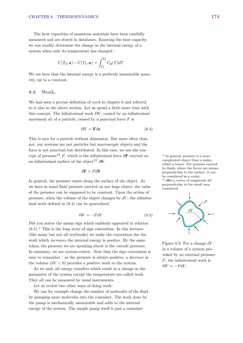
CHAPTER 8. THERMODYNAMICS. 174
The heat capacities of numerous materials have been carefullymeasured and are stored in databases. Knowing the heat capacity,we can readily determine the change in the internal energy of asystem when only its temperature has changed :
U(T2, a)−U(T1, a) =ˆ T2
T1
Ca(T )dT
We see here that the internal energy is a perfectly measurable quan-tity, up to a constant.
8.6 Work.
We had seen a precise definition of work in chapter 6 and referredto it also in the above section. Let us spend a little more time withthis concept. The infinitesimal work δW , caused by an infinitesimalmovement dx of a particle, caused by a punctual force F is
δW = Fdx (8.4)
This is nice for a particle without dimension. But more often thannot, our systems are not particles but macroscopic objects and theforce is not punctual but distributed. In this case, we use the con-cept of pressure14 P , which is the infinitesimal force dF exerted on 14 In general, pressure is a more
complicated object than a scalar,called a tensor. For pressure exertedby fluids, where the forces are alwaysperpendicular to the surface, it canbe considered as a scalar.
an infinitesimal surface of the object15 dS:
15 dSis a vector of magnitude dSperpendicular to the small areaconsidered
dF = PdS
In general, the pressure varies along the surface of the object. Aswe have in mind fluid pressure exerted on not huge object, the valueof the pressure can be supposed to be constant. Upon the action ofpressure, when the volume of the object changes by dV , the infinites-imal work defined in (8.4) can be generalized
Figure 8.3: For a change dVin a volume of a system pro-voked by an external pressureP , the infinitesimal work isδW = −PdV .
δW = −PdV (8.5)
Did you notice the minus sign which suddenly appeared in relation(8.5) ? This is the long story of sign convention. In this lectures(like many but not all textbooks) we make the convention the thework which increases the internal energy is positive. By the sametoken, the pressure we are speaking about is the outside pressure.In summary, we are system-centric. Note that the sign convention iseasy to remember : as the pressure is always positive, a decrease inthe volume (dV < 0) provides a positive work to the system.
As we said, all energy transfers which result in a change in theparameter of the system except the temperature are called work.They all can be measured by usual instruments.
Let us review two other ways of doing work.We can for example change the number of molecules of the fluid
by pumping more molecules into the container. The work done bythe pump is mechanically measurable and adds to the internalenergy of the system. The simple pump itself is just a container

175 8.6. WORK.
with two gates, and a moving piston which at each cycle, send Nmolecules of the outside reservoir fluid into the main container.From the discussion above, we know that the work done by thepump at each cycle is
Figure 8.4: Pumping moleculesinto a container
δW = −PdV
where −dV is the volume of the pump and P the outside pressurenecessary to move down the piston. We’ll come back to this examplewhen we learn more about gasses.
Or consider a thermally isolated capacitor (see 7.4.2) as your sys-tem (figure 8.5). You can change the charges in your capacitor byconnecting it to a DC power source with electric potential V , anddisconnect it when the capacitor is charged. You can measure pre-cisely by electrical means the work done by your power source bymonitoring the current I(t) which flows into the circuit and deter-mine the amount of work (energy transfer) you have performed:
W =
ˆ ∞0
V .I(t).dt
§ 8.9 Work to charge a capacitor. Using the electricity concepts seen in sub-section 7.4.2, compute the current I(t) in the circuit and the work performedby the power source (figure 8.5).
Figure 8.5: Charging a capaci-tor.
Solution. Let VR and VC be the potentials around the resistor and thecapacitor. We know that
VR + VC = V (8.6)
Let I be the current in the circuit. From basic relations of the electricity, wealso have
VR = RI ; dVCdt
=1CI (8.7)
As the power source potential is constant, by deriving relation (8.6) andplugging it into relation (8.7) we get
0 2 4 6 8 10
0.0
0.2
0.4
0.6
0.8
1.0
1.2
1.4 (a)
I
Vc
0 2 4 6 8 10
t0.0
0.2
0.4
0.6
0.8
1.0
1.2
(b)
P
Pc
Figure 8.6: Charging a ca-pacitor connected to a powersource. (a) the current I(t) andthe capacitor potential Vc(t).(b) the power P (t) = I(t)V (t)
provided by the source andPc(t) = I(t)Vc(t) transmittedto the capacitor. The shadedarea below each curve representthe respective work.
dI
dt= − 1
RCI
and thereforeI(t) = Ae−t/τ (8.8)
where τ = RC. Integrating one more the above equation, and using theboundary conditions V2(0) = 0 and V2(∞) = V , we get
VC (t) = V (1− e−t/τ )
and A = V /R.So, we know the current and the potential in the circuit at any time. The
work received by the capacitor is therefore
Wc =
ˆ ∞0
VC (t)I(t)dt =12CV
2
On the other hand, the work provided by the power source is
W =
ˆ ∞0
V .I(t)dt = CV 2
Note that in the condenser system example we examined, the re-sistor was placed outside the system. This is an ideal model, anycapacitor has also an internal electrical resistance, so in real systems,
CHAPTER 8. THERMODYNAMICS. 176
the resistor should be considered inside the system. You have no-ticed that the capacitor has received only half of the work done bythe power source. Where did the other half disappear ? The answerresides in the warming of the resistor. If the resistor is in thermalcontact with the outside world, it will transfer this work to the out-side world as heat. If the system formed by the capacitor and theresistor are thermally isolated, they will increase their temperatureand store this work as their internal energy. The full answer to thisquestion is the subject of the next section.
We have examined here few examples of providing energy to asystem by work. In all the physical system work involves movingobjects and is always measurable by electrical or mechanical instru-ments. More over, as we know the physics of these systems, we canalso theoretically estimate the amount of work necessary to changethe parameters (volume, number of molecules, ...) of the system.
Summary.The internal energy of system U can be changed by energy transfersfrom the outside which are called work W or heat Q. The change inthe internal energy exactly equals the amount of energy transfer:
∆U = W +Q
Heat involves putting the system in contact with another hotter orcolder system, whitout changing any of the extensive variables of thesystem. Work involves moving objects and change of the extensiveparameters of the system. All energy transfer are perfectly measur-able; therefore, the internal energy of a system is a known quantity,up to constant.The above statement is called “the first principle of thermodynam-ics”.
8.7 Equilibrium, reversible and irreversible changes.
A system is in equilibrium when all macroscopic measurements ofthe quantity of the system remain constant. Consider for example aliquid or a gas in a reservoir. We can constantly monitor its variousparameters (number of molecules, volume, pressure ...). If all theparameters we can measure remain constant, we say that the fluid orthe gas is in equilibrium.
Suppose now that we change some parameters, say the volume V(for example, by compressing the gas). Then other parameters willalso change ; the change in other parameters is not spontaneous, butafter some time τ , all other parameters will again reach a stationaryvalue and remain there. The time it takes for the system to reach anew equilibrium is called its relaxation time. By making this change,we have moved the system from one equilibrium state to anotherone.
The changes brought to a system can be fast or slow compared to

177 8.8. ENTROPY.
the relaxation time. If the parameter a has changed by ∆a, a slowchange means that
da
dt ∆a
τ
during a slow change, the system is always in equilibrium ; on theother hand, during a fast change, the system is at equilibrium onlyat the beginning and at the end process, but not in between. Wewill call the infinitely small changes reversible changes, and the fastchanges irreversible.
irrev
rev
Figure 8.7: irreversible vs re-versible transformation. whena system is perturbed, its pa-rameters evolve from a valuea to reach a new equilibriumvalue a+ ∆a over a time scale τcalled the relaxation time (bluecurve). A reversible processbrings the same changes to thesystem on a much slower timescale (red curve). The slope ofthe variation in the reversiblecase (da/dt) is much smallerthan ∆a/τ .
To illustrate the difference between these two types of changes,let us consider again the charging of the capacitor. In exercise 8.9,we suddenly changed the state of the system by connecting it to aconstant power source V . The relaxation time there was τ = RC
; however, the current I suddenly jumped at time t = 0 from zeroto V /R. This is what we call a fast or irreversible change. What wesaw is that the power source provided a work of W = CV 2, whilethe capacitor received a work of W = (1/2)CV 2: half the workprovided by the power source was dissipated as heat. Now let usconsider a slow change.
§ 8.10 Work to charge a capacitor, reversile . Connect the same system asdepicted in figure 8.5 to a variable power source V (t) = V0 (1− exp(−ω0t)).Compute the current I(t) and the potential Vc(t). Deduce the work receivedby the capacitor and the work performed by the power source in the limitω0 → 0.
Solution. An easy but cumbersome computation will lead to
I(t) =V0ω0
R(ωc − ω0)
(e−ω0t − e−ωct
)where ωc = 1/(RC). Integrating one more time, we have
Vc(t) = V0 + V0ω0ωcωc − ω0
(e−ωct
ωc− e−ω0t
ω0
)when ω0 → 0 (i.e. ω0 ωc), Vc(t) ≈ V (t) and therefore, Wc ≈ W : all thework provided by the power source is transmitted to the capacitor. Computingexplicitely the work, we find that
Wc ≈W =12CV
20
Note that the electrical internal energy of a capacitor at potential V0 isUelec = (1/2)CV 2, so all the work has been used to increase the electricinternal energy.
8.8 Entropy.
The concept of entropy appeared formally in 1830 in the work ofSadi Carnot16. From the beginning of thermal machines, it was 16 Réflexions sur la puissance motrice
du feu.evident that energy transfer to a system is wasteful: Whatever meanyou use to transfer energy to a system, the amount of work thesystem can give back is always inferior to the amount of energy yougave to it in the first place if heat has been implied. For a time,people believed that by improving the machines, the yield can beincreased and ideally reach one. Carnot showed that this is not going

CHAPTER 8. THERMODYNAMICS. 178
to be, and the ideal thermal machine will always under-perform.Carnot arrived at this conclusion by an incredibly beautiful thoughtexperiment17 which we are not going to explain until we’ll learn 17 The experiment involves a cycle of
gas heating and compression, whichis known as the Carnot cycle.
more about gases. However, let us consider the first principle again,by moving the δQ term to the other side:
δW = dU − δQ
It appears that the amount of work we can get from a system is lessthan the change in its internal energy, but in a very predictable way,and is of the form
F = U − TS
where U is the internal energy, T is the temperature and S a quan-tity called entropy. The entropy is a quantity similar somehow tothe internal energy, in the fact that its value depends only on thetemperature and the parameter a of the system
S = S(T , a)
We saw earlier that changes in the internal energy are perfectlymeasurable. The changes in the entropy are also measurable and aregiven by
dS =δQ
Tprovided that the change brought to the system is reversible. Wecan always compute the change of the entropy when the change isirreversible by imagining a reversible process which brings the samechanges to the same parameters.
Consider the capacitor we studied before. Its internal energy is afunction of temperature and its potential
U = U(T ,V )
and of course, the entropy S = S(T ,V ). We saw however that wecan charge reversibly the capacitor without involving any heat, andtherefore S = S(T ), i.e. the entropy does not depend on the chargesof the capacitor.
8.9 Application to Perfect gases.
In order to get familiar with the concepts we developed in the abovesections, we will no study the perfect gas example. A gas in a con-tainer has only two extensive parameters : its volume V and thenumber of molecules N . As the number of molecules is huge, wemeasure it in mole n, i.e. in unit of Avogadro number NA. There-fore, both the internal energy and entropy are only function of thesetwo parameters and the temperature:
U = U(T ,V ,n) ; S = S(T ,V ,n)
By the same token, all other property of the gas are also function ofthese sets of parameters. For example, the gas pressure is
P = P (T ,V ,n) (8.9)
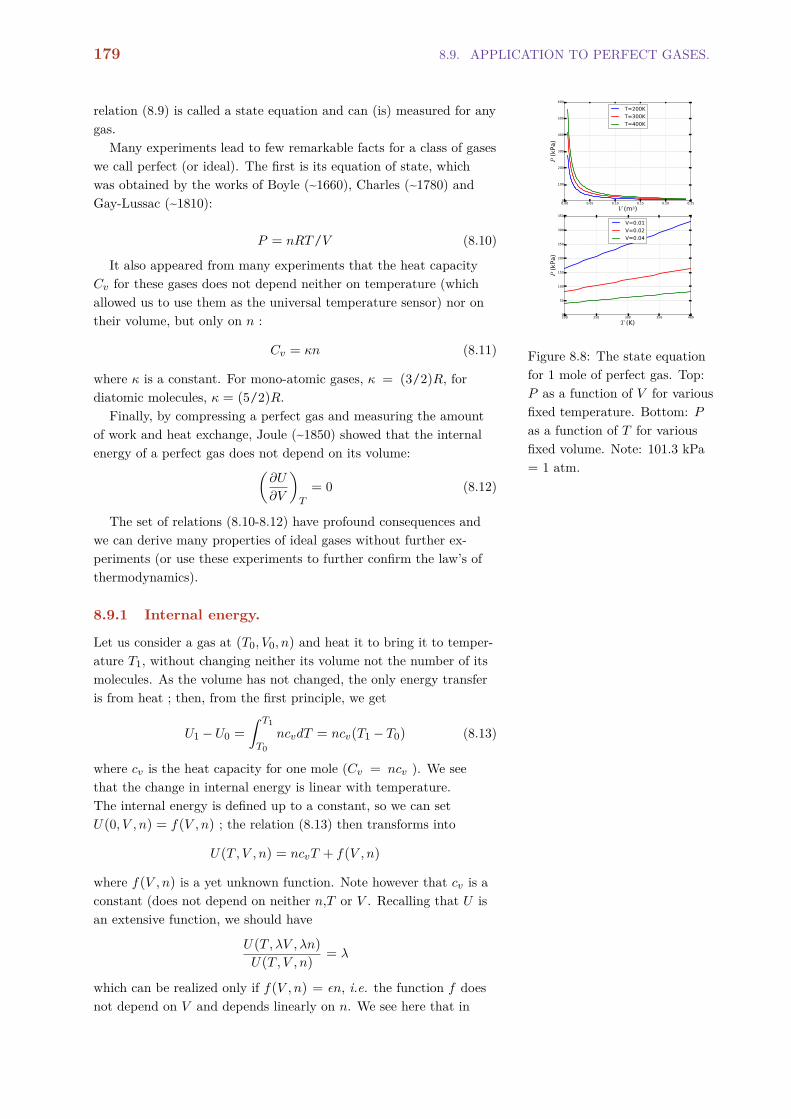
179 8.9. APPLICATION TO PERFECT GASES.
relation (8.9) is called a state equation and can (is) measured for anygas.
Many experiments lead to few remarkable facts for a class of gaseswe call perfect (or ideal). The first is its equation of state, whichwas obtained by the works of Boyle (~1660), Charles (~1780) andGay-Lussac (~1810): 0.00 0.05 0.10 0.15 0.20 0.25
V (m3)0
100
200
300
400
500
600
P (k
Pa)
T=200KT=300KT=400K
200 250 300 350 400T (K)
0
50
100
150
200
250
300
350
P (k
Pa)
V=0.01V=0.02V=0.04
Figure 8.8: The state equationfor 1 mole of perfect gas. Top:P as a function of V for variousfixed temperature. Bottom: Pas a function of T for variousfixed volume. Note: 101.3 kPa= 1 atm.
P = nRT/V (8.10)
It also appeared from many experiments that the heat capacityCv for these gases does not depend neither on temperature (whichallowed us to use them as the universal temperature sensor) nor ontheir volume, but only on n :
Cv = κn (8.11)
where κ is a constant. For mono-atomic gases, κ = (3/2)R, fordiatomic molecules, κ = (5/2)R.
Finally, by compressing a perfect gas and measuring the amountof work and heat exchange, Joule (~1850) showed that the internalenergy of a perfect gas does not depend on its volume:(
∂U
∂V
)T
= 0 (8.12)
The set of relations (8.10-8.12) have profound consequences andwe can derive many properties of ideal gases without further ex-periments (or use these experiments to further confirm the law’s ofthermodynamics).
8.9.1 Internal energy.
Let us consider a gas at (T0,V0,n) and heat it to bring it to temper-ature T1, without changing neither its volume not the number of itsmolecules. As the volume has not changed, the only energy transferis from heat ; then, from the first principle, we get
U1 −U0 =
ˆ T1
T0
ncvdT = ncv(T1 − T0) (8.13)
where cv is the heat capacity for one mole (Cv = ncv ). We seethat the change in internal energy is linear with temperature.The internal energy is defined up to a constant, so we can setU(0,V ,n) = f(V ,n) ; the relation (8.13) then transforms into
U(T ,V ,n) = ncvT + f(V ,n)
where f(V ,n) is a yet unknown function. Note however that cv is aconstant (does not depend on neither n,T or V . Recalling that U isan extensive function, we should have
U(T ,λV ,λn)U(T ,V ,n) = λ
which can be realized only if f(V ,n) = εn, i.e. the function f doesnot depend on V and depends linearly on n. We see here that in

CHAPTER 8. THERMODYNAMICS. 180
fact, Joule’s second law (relation 8.12) is a consequence of relation(8.11) and simple thermodynamics considerations.
We see that the general form of the internal energy of a perfectgas is
U = n(cvT + ε) (8.14)
8.9.2 Entropy.
Let us first heat the gas at constant volume as in the precedingsubsection. As
δQ = ncvdT
the entropy change during this transformation is
S(T1,V ,n)− S(T0,V ,n) = ncv
ˆ T1
T0
dT
T= ncv log
(T1T0
)(8.15)
Let us now compress the gas at constant temperature (isothermalcompression). We do that by letting the piston compressing thegas to move very slowly (reversible transformation) : at each timestep, we change the external pressure by a small amount dP . As thetransformation is reversible, the internal and external pressure arealways equal. The work received by the system is
W = −ˆ V1
V0
pdV = −nRTˆ V1
V0
dV
V
= −nRT log(V1V0
)during the compression process, there is also heat exchange Q withthe outside world. In this transformation, T and n are constant andonly the volume has changed. On the other hand, we know thatthe internal energy U does not depend on V , so U has remainedconstant during this transformation. But ∆U = Q+W = 0 so
Q = nRT log(V1V0
)and because the temperature has remained constant,
S(T ,V1,n)− S(T ,V0,n) = nR log(V1V0
)(8.16)
Combining relations (8.15,8.16) we thus find that
S(T1,V1,n)− S(T0,V0,n) = ncv log(T1T0
)+ nR log
(V1V0
)(8.17)
We can further re-arrange the above equation as
S = nR log(V T cv/R
g(n)
)(8.18)
where g(n) is a function of n only.
§ 8.11 Show that relation (8.17) can indeed be obtained from (8.18).

181 8.9. APPLICATION TO PERFECT GASES.
§ 8.12 Using the extensivity of S, demonstrate that g(n) must be linear inN , i.e. g(n) = φn where φ is a constant and therefore
S = nR log(V T cv/R
φn
)(8.19)
§ 8.13 Demonstrate that when T → 0, S → −∞ for a perfect gas. Usually,we expect the entropy to approach zero when temperature is decreased. Howthis contradiction can be explained ? Do you know any gas which does notliquefy at low temperature ?
§ 8.14 Imagine an infinitesimal transformation where dn mole of perfect gasis pushed into a container at (T ,V ,n) of the same gas. The gas is in thermalequilibrium with a reservoir. The pump pushes a volume dV = (V /n)dn intothe container. What is the work δW received by the system ?
Using the expression for the internal energy U = ncv(T + ε), computethe change in internal energy dU and the heat δQ received by the system.Deduce the change dS in entropy. Finally, compute directly the change inentropy due to the change in n from expression (8.19). Deduce a relationbetween φ and ε.
8.9.3 Mathematical detour: constraints and differen-tials.
It is worthwhile to clarify a mathematical point. Consider a two di-mensional space where points are referred to by two coordinates x, y.Let us be on a point (x0, y0) and make a small movement (dx, dy)around this point, bringing us to (x0 + dx, y0 + dy). This is a freeworld so we can do any movement we like.
Let us now add a constraint. We ask for the points we are inter-ested in to satisfy a given relation f(x, y) = 0. Geometrically, thismeans that we consider only points on a given curves. For example,if f(x, y) = x2 + y2 − 1, the points have to lie on a circle of radius1 around the origin. Now consider again a point (x0, y0) satisfyingthe constraint and let us make a move (dx, dy) around this pointthat keeps us on the curve. Obviously, this time, we cannot make anarbitrary move, but dx and dy have to satisfy some relation, i.e. wemust have
f(x0 + dx, y0 + dy) = 0
Developing the above relation to the first order, we have(∂f
∂x
)x0,y0
dx+
(∂f
∂y
)x0,y0
dy = 0 (8.20)
This means that dx and dy are linearly related: knowing either dx ordy will determine the value of the other component of displacementwhich keeps us on the curve.
Figure 8.9: Allowed small dis-placements (red arrows) aroundvarious points on the circle.
§ 8.15 For the curve x2 + y2 − 1 = 0 (figure 8.9), determine the relationshipbetween dx and dy for the points (1, 0),(
√2/2,
√2/2),(0, 1),(−
√2/2,
√2/2).
Solution. for f(x) = x2 + y2 − 1, we have ∂xf = 2x and ∂yf = 2y.At the point (1, 0), ∂xf = 2 and ∂yf = 0 so the relation (8.20) reduces to2dx+ 0dy = 0 or dx = 0. For the point (1, 0), small displacements must bevertical.

CHAPTER 8. THERMODYNAMICS. 182
At the point (√
2/2,√
2/2), ∂xf =√
2 and ∂yf =√
2 so the rela-tion (8.20) reduces to
√2dx +
√2dy = 0 or dx = −dy. For the point
(√
2/2,√
2/2), small displacements must be at −π/4. The reader will com-plete the other points.
The above considerations extends naturally to spaces of higher di-mensions. For a three dimensional space (x, y, z), where points mustsatisfy a constraint f(x, y, z) = 0 for example, the small displace-ments (differentials) must satisfy(
∂f
∂x
)x0,y0,z0
dx+
(∂f
∂y
)x0,y0,z0
dy+
(∂f
∂z
)x0,y0,z0
dz = 0
§ 8.16 For a perfect gas at (P ,V ,T ), what is the relation between smallchanges dP , dV , dT ? Consider further particular displacements of the formdP = 0 (isobar) or dV = 0 (isovolume) or dT = 0 (isotherm).
Solution. The constraint function for a perfect gas (the state equation) is
f(P ,V ,T ) = PV
T− nR
and therefore ∂P f = V /T , ∂V f = P/T , ∂T f = −PV /T 2. The differen-tials must then satisfy
(V /T )dP + (P/T )dV − (PV /T 2)dT = 0
the above equation can be rearranged using the state equation into
dP
P+dV
V− dT
T= 0 (8.21)
For an isobar transformation (a transformation at constant pressure), dP = 0so we must have dV /V = dT/T . For an isotherm transformation, dT = 0and we must have dP/P = −dV /V .
8.9.4 Heat capacity at constant pressure.
We defined the heat capacity Cv as the amount of heat δQ necessaryin order to increase the temperature by dT at constant volume:δQ = CvdT . To measure it, we heat the gas when the volume isfixed and measure simultaneously the heat δQ and the temperatureincrease dT and form their ratio.
But we can do the heating at constant pressure, letting the vol-ume vary. For this, we use a movable piston on top of our container,which is thermally isolated from the outside: as the gas is heated,the volume increase but the pressure inside the gas remains con-stant and equal to the outside pressure Pext. The heat capacity Cp isdefined again by
Figure 8.10: Heating at con-stant pressure: a thermallyisolated cylinder with a mov-able piston containing a gas isheated to bring its temperatureto T1 from T0. For small tem-perature change, Cp is definedas δQ/dT .
Cp =δQ
T
What is the relation between Cp and Cv ? Note that by heating, wehave changed the state of the system from T ,V ,n to T + dT ,V +
dV ,n. The work done during this process is
δW = −PextdV

183 8.9. APPLICATION TO PERFECT GASES.
on the other hand, the gas is always at equilibrium (reversible pro-cess done slowly) and the inside and outside pressure are equal andconstant. So from the state equation V = nRT/P , we deduce (see§8.16) the relation between volume and temperature change:
dV =nR
PdT
and therefore the work during the transformation is
δW = −nRdT
and the change in internal energy is
dU = δW + δQ = (Cp − nR)dT (8.22)
However, from relation (8.13), we also know that the change in inter-nal energy for the process (T ,V ,n)→ (T + dT ,V + dV ,n) is
dU = CvdT (8.23)
and comparing relation (8.22,8.23), we deduce
Cp −Cv = nR
or writing these relations for one mole, we have
cp − cv = R
We see here that without doing the experiment, we can determinethe value of cp, which is also independent of volume. Of course,many thousand of experiment will confirm this result.
8.9.5 Adiabatic compression.
Consider a perfect gas in a container with a movable piston. At theinitial moment, the outside pressure is P0 , the volume V0 and thetemperature T0. We compress the gas adiabatically (the containeris thermally isolated) by increasing the pressure to P1. Obviously,both the volume and the temperature will change to V1 and T1. Thestate equation PV = nRT cannot gives us the value of both V1 andT1, but only their ratio. Can we do any better and determine thesevalues from thermodynamic considerations ?
Consider an infinitesimal part of this transformation, when thepressure is changed from P to P + dP . The amount of work duringthis process is
δW = −PdV
but because no heat has been exchanged with the outside (δQ = 0),we must have
Figure 8.11: Adiabatic com-pression of a thermally isolatedgas by changing the outsidepressure from P0 to P1.
dU == δW = −PdV (8.24)
on the other hand, we know that when a perfect gas changes itsvolume and temperature by dV and dT , its internal energy changesby (relation 8.13):
dU = CvdT (8.25)

CHAPTER 8. THERMODYNAMICS. 184
combining relations (8.24,8.25), we therefore must have
−PdV = CvdT (8.26)
Which gives us another constraint on the small displacements dVand dT .
Let us think a little more about what we have done. in exercise§8.16, we obtained one relation (8.21) between differentials by ex-ploiting the contraint that the gas must be perfect (i.e. obey thestate equation PV = nRT ). In the problem we are studying now,we ask the small displacements to be not only in agreement withthe constraint of the perfect gas, but also with the constraint of thetransformation being adiabatic. This further constraint gives us an-other relation (8.26) between the differentials, which we can exploit.Relation (8.21) by itself is not enough, as we don’t know the value ofV and T during the transformation.
We can now rearrange slightly relation (8.26) by using again thestate equation and the specific (molar) heat capacity cv = Cv/n:
dT
T= −R
cv
dV
V(8.27)
The quantity R/cv = (cp − cv)/cv is often written as (γ − 1) whereγ = cp/cv is called the heat capacity ratio or the adiabatic index.
Note that relation (8.27) involves only V and T and not P . It is asimple differential equation ; integrating both side, we find a relationbetween V and T at any point along the adiabatic transformation
T
T0=
(V
V0
)−(γ−1)
which can be rearranged into
TV γ−1 = T0Vγ−1
0 = Cte (8.28)
or by using the state equation, into
PV γ = P0Vγ
0 (8.29)
Obviously, the above relation allows for the determination of thevolume of the gas at the end of adiabatic compression (when thepressure reaches P1) and the temperature.
§ 8.17 Show that an adiabatic expansion leads to the cooling of perfectgases.
§ 8.18 Show that expression (8.28) is compatible with the expression ofentropy (8.19) : no change occurs in the entropy during adiabatic expansion.
8.9.6 Joule expansion.
Consider a gas in a half chamber of a thermally isolated cylinder.Open now a small valve and let the gas fill the whole cylinder. Howthe temperature of the gas is changed ?
Note that we have changed the state from (P0,V0,T0) to (P1,V1 =
2V0,T1) and again the state equation is not enough to determine the

185 8.10. THE THERMAL MACHINE: CARNOT CYCLE.
final temperature as the final pressure is not known. However, nowork has been exchanged with the outside (W = 0) as the volume ofthe cylinder has not changed. By the same token, no heat has beenexchanged neither (Q = 0) with the outside world as the cylinder isthermally isolated. Therefore ∆U = 0.
Figure 8.12: Free expansion. Avalve is opened in the wall sep-arating the two half chambers,allowing the gas in the firsthalf chamber to fill the wholecylinder.
On the other hand, we know that for a perfect gas, ∆U = Cv∆Twhich lead us to conclude that ∆T = 0, i.e. there is no temperaturechange and doubling the volume with this transformation has onlyhalved the pressure.
So what has changed ? A quick look at expression (8.17) showsthat
∆S = nR log 2 (8.30)
§ 8.19 Not heat has been exchanged with the outside ; however, the entropyhas increased. Is this statement in contradiction with the computation ofentropy change dS = δQ/T ? Can you imagine a reversible process whichproduces the same changes in the extensive variables ?
Let us finally note that many real gases (not ideal gases) willcool upon free expansion, and this is indeed used as a refrigerationmethod, specially at very low temperature. Some gases will gethotter upon free expansion.
8.9.7 Perfect gas: conclusion.
The first sections of this chapter were dedicated to fundamentalprinciples of thermodynamics. The present section contained theapplication of these principles to a very simple system: the perfectgas. Let us think why we spend few pages on perfect gases.
The perfect gas is a very simple system. We presented two exper-imental facts of these systems: their state equation PV = nRRT
and the heat capacity measurement. From only these set of mea-surements and the knowledge that we have two abstract quantitiesU and S, we derived a wealth of new relations such as the relationbetween cp and cv , the form of the adiabatic expansions, ...
This is the general procedure of thermodynamics that applies toany physical system. Thermodynamics is not a magical tool, we doneed to measure some relations (such as the state equation) of thephysical system under investigation. But when the correct expres-sions for work and heat are formulated for the particular system, awealth of new relations can be deduced by the same kind of reason-ing we developed in this section. Another formulation would be thatthermodynamics limits the freedom in the values of many propertiesof the system, binding them together through simple formulation.It takes some practice to tame the power of this procedure, but thefundamental principles are extremely simple and elegant.
8.10 The thermal machine: Carnot cycle.
Humans have had few inventions that have radically modified theirhistory and allowed for huge increase in their population number.

CHAPTER 8. THERMODYNAMICS. 186
The invention of agriculture around 10000 years ago is one of them.The next invention with comparable impact was the thermal ma-chine. Contrary to the agricultural invention, we know the inventorand the date of the first heat engine: Newcomen and 1712. Until thisdate, humans knew how to harness the energy of few sources such asanimals, wind and rivers to perform work. After this date, they har-nessed the chemical (and later nuclear) energy stored in earth mantlein the form of coal, oil (and later uranium).
Figure 8.13: The Newcomensteam engine. (source: Wikiperdia)
The Newcomen steam engine worked on the following principle:Take a cylindric container with a movable piston and put some wa-ter inside. Boil the water to make steam whose pressure would pushthe piston upward. Then cool suddenly the cylinder to transformback the steam into water, which would bring the piston to its orig-inal, lower position. The heating was provided by burning coal, thecooling was provided by injecting cold water into the cylinder. Theprocess was automated to open and close the valves at appropriatetime.
James Watt improved the Newcomen machine in 1770 by a smartdevice which avoided to cool the whole metallic cylinder at eachcycle: the same amount of coal would produce much higher workthan in the Newcomen machine.
A large number of engineer then followed the footsteps of Wattand tried to improve the efficiency of the heat engine. We are pro-viding an amount of Q heat to the system and getting an amount Wof work from it. Can we get very efficient machines in which W = Q
? Or a perpetual machine in which W > Q ?The answer to these questions came in 1830 in the book of Saadi
Carnot : the most efficient thermal machine will always have η =
W/Q < 1. Even better, the best bithermal machine (functioningat two different hot and col temperature such as the Newcomenmachine) would have η = 1− Tc/Th. The work of Carnot laid one ofthe foundation of thermodynamics and led to the concept of entropyand absolute temperature.
As we are not interested in the historical development of thermo-dynamics in these lectures, we will use the concepts developed in thefirst part of this chapter to study the Carnot reversible machine.
Figure 8.14: C1: Isothermalcompression.
The Carnot machine is again a cylinder containing a gas and amovable piston. Let us suppose that at the beginning of the cycle,the gas is at Tc,V0,P0. The gas does not need to be perfect and canhave any state equation f(T ,V ,P ) = 0.
1. The gas is compressed isothermally by increasing the outsidepressure from P0 to P1(fig. 8.14). During the whole transforma-tion, the cylinder is in thermal contact with a cold reservoir at Tc.We can summarize this transformation by
Tc,V0,P0 → Tc,V1,P1
where P1 > P0 and V1 < V0.
Figure 8.15: C2: Adiabaticcompression.
2. The cylinder is now thermally isolated from the cold reservoir.

187 8.10. THE THERMAL MACHINE: CARNOT CYCLE.
We continue to increase the pressure to P2, adiabatically com-pressing the gas to volume V2 until it reaches the temperatureTh:
Tc,V1,P1 → Th,V2,P2
where Th > Tc, P2 > P1 and V2 < V1
3. Until now, we were giving work to the system. We now beginto extract work from it. We put the cylinder in thermal contactwith a reservoir at Th, decrease the pressure to P3 and let the gasexpand to V3 isothermally:
Figure 8.16: C3: Isothermalexpansion.
Th,V2,P2 → Th,V3,P3
where P3 < P2 and V3 > V2.
4. We again isolate the cylinder from the hot reservoir, decrease thepressure adiabatically to P0 where we are back again to tempera-ture Tc and volume V0:
Figure 8.17: C4: Adiabaticexpansion
Th,V3,P3 → Tc,V0,P0
§ 8.20 Explain why during the fourth part of the cycle, we are back to Tcand V0. More precisely, would any choice of P3 grant a safe return to Tc andV0 ?
Let us know analyze this cycle. The variation of P and V aredepicted in figure 8.18. During the C1 part of the cycle, dV < 0so the system is receiving the work W1 > 0. As the system is notthermally isolated, it also receives a heat Q1. In fact, in absoluteterm, the system is providing heat to the outside, so Q1 < 0.
§ 8.21 Explain why Q1 < 0.
The variation of internal energy is ∆U = U1 − U0 = W1 + Q1and the variation of the system’s entropy is ∆S = S1 − S0 = Q1/Tc.We stress that during this leg of the cycle, the temperature remainsconstant so ∆S =
´ 10 δQ/T = (1/Tc)
´ 10 δQ = Q1/Tc.
During the C2 part of the cycle, still dV < 0 so the system is stillreceiving the work W2 > 0. As the system is thermally isolated, itreceives no heat. The variation of internal energy is ∆U = U2 −U1 =
W2 and the variation of the system’s entropy is ∆S = S2 − S1 = 0.
Figure 8.18: Carnot cycleP − V diagram. The work per-formed by the machine equalsthe shaded area.
During the C3 part of the cycle, dV > 0 so the system is provid-ing the work W3 < 0. The system is again not thermally isolated,therefore it receives the heat Q3. This time, in absolute term, thesystem is receiving heat from the outside, so Q3 > 0. The variationof internal energy is ∆U = U3 − U2 = W3 +Q3 and the variation ofthe system’s entropy is ∆S = S3 − S2 = Q3/Th.
Finally, during the C4 part of the cycle,still dV > 0 so the sys-tem is providing the work W4 < 0. The system is again thermallyisolated, therefore it exchanges no heat. The variation of internalenergy is ∆U = U0 − U1 = W4 and the variation of the system’sentropy is ∆S = S0 − S3 = 0.

CHAPTER 8. THERMODYNAMICS. 188
We have now come full circle: as U and S depends only on theparameters of the system, their total variation must be exactly zero.For the entropy, we have
∆Stotal =Q1Tc
+Q3Th
= 0 (8.31)
from which we conclude that, in absolute term,
Figure 8.19: The carnot cyclein S − T diagram. The totalamount of heat Q =
¸TdS
is represented by the shadedarea of the surface. Because ofthe direction the of the cycle,Q > 0 and W = −Q < 0.
|Q1|Tc
=|Q3|Th
(8.32)
This is an extraordinary relations which we obtained with no cal-culation or experiment. Note that because Th > Tc, we must alsohave
|Q3| > |Q1| (8.33)
.Let now W = W1 +W2 +W3 +W4 be the total work received by
the system. For the full cycle,
∆Utotal = W +Q1 +Q3 = 0
or in other terms,W = −(Q1 +Q3)
We know that Q1 < 0 and Q3 > 0, therefore, using relation (8.33) wededuce that
W < 0
in other terms, the machine is indeed providing work to the outsidewhich can be used to pump water in the mine or move the locomo-tive.
What we are interested is the efficiency of the machine. The ma-chine has received the heat Q3 and the provided the total work W .The efficiency is
η =|W |Q3
= 1 + Q1Q3
and using relation (8.31), we therefore have Figure 8.20: The bithermalengine can be envisioned as aheat flow between a hot andcold sources ; part of the flowis converted into work by thesystem (engine).
η = 1− TcTh
(8.34)
This is an extraordinary conclusion. First, the efficiency of theCarnot machine does not depend on the kind of gas we have used :it depends only on the ratio of temperatures of hot and cold sources.Second, this is the best bithermal machine we could make. We canimagine other type of cycles, but all of them would have (as long asthey are reversible like Carnot machine) the same efficiency. If theyhad better efficiency, we could couple this machine with the Carnotmachine and make a perpetual machine.
Finally, note that the efficiency of the machine is 0 if Tc = Th: wecannot have a mono-thermal thermal machine. On the other hand,the efficiency is enhanced when the ratio Th/Tc is increased. This iswhy material engineers spend tremendous research to find materialscapable of sustaining very high temperature that can be used inturbines at higher and higher temperature.

189 8.11. THE THERMODYNAMIC POTENTIAL F AND THE MINIMUM PRINCIPLE.
8.11 The thermodynamic potential F and theminimum principle.
8.11.1 The Helmholtz free energy.
The (Helmholtz) free energy F is defined generally as
F = U − TS
as U and S depend only on the parameter of the system (such asT ,V ,N), so does F :
F = F (T ,V ,N)
We express this fact by saying that F (and U and S ) is a statefunction. The fact that it is called free energy is because when thestate of the system (the parameter T ,V ,N ,...) are changed fromstate 1 to state 2, the amount of work we can get from (or provideto) the system is W = F2 − F1.
§ 8.22 using the expressions
U = n(cvT + ε) (8.35)
andS = nR log(V T cv/R/φn) (8.36)
of the perfect gas, verify that the work in each leg of the Carnot cycle of aperfect gas indeed corresponds to the work received by the system.
It appears that F , which is called a thermodynamic potential,plays a much more important role than just the amount of ex-tractable work. Let us for example compute the variation in F dueto a variation in V for a perfect gas, keeping all other parametersconstant. We see that, for a perfect gas whose internal energy doesnot depend on the volume,
∂F
∂V= −T ∂S
∂V= −TnR/V = −P
the fact thatP = −∂F
∂V
is not a coincidence! indeed, this is the general definition of thequantity we call pressure.
We can compute other derivative of F , for example in respect toT :
∂F
∂T=∂U
∂T− T ∂S
T− S
and a close inspection of relations (8.35,8.36) shows that ∂TU andT∂TS exactly cancel each other ; in other terms,
S = −∂F∂T
(8.37)
and again, this is a general expression, not limited to perfect gases.
§ 8.23 Verify (demonstrate) the validity of (8.37) for perfect gases.

CHAPTER 8. THERMODYNAMICS. 190
In general, letF = F (a1, a2, ..., an)
the quantity Ai = −∂F/∂ai is called the generalized force conju-gated (associated) to ai (for some quantity, the + (plus) sign is usedfor historical reasons) . For ai = T , the generalized force is calledthe entropy S; for ai = V , the generalized conjugated force is thepressure P ; for ai = n, the generalized force is called the chemicalpotential µ (For which the + sign is used). A small change dai in theparameter of the system will cause a change dF in the free energy
dF =∑(
∂F
∂ai
)dai
for example, if the system is a gas (ideal or real), we have
dF = −PdV + µdn− SdT
In fact, F is the fundamental quantity in thermodynamics, and allother state functions such as U and S are defined in terms of F andits derivative18. For example, based on what we said above, 18 We use the term fundamental to
stress that when thermodynamics isderived from molecular principle, Fis the quantity which is stated as thebasic principle. A system in thermalequilibrium with a reservoir is alwaysfluctuating at the microscopic level; these fluctuations are small andtherefore are not measurable at themacroscopic level. So a system canbe found in any state η. However,the probability of observing thesystem in state η with the energy Eηis given by
Prob(η) = (1/Z)e−Eη/kT
were Z is a normalizing constant inorder for the sum of probabilitiesto be equal to unity. The abovestatement is the only axiom we needto derive the whole thermodynamicsfrom microscopic considerations. Thefree energy is defined as
F = −T logZ
Reader interested in this topic is re-ferred to any textbook on statisticalphysics.
U = F − T ∂F∂T
So if we know F (T ,V ,n), we can determine both U and S.
8.11.2 The minimum principle.
Consider a metal bead in a bowl filled with a fluid such as water.We can let the bead at any position in the bowl at the beginning, wewill find the bead in the bottom of the bowl after some time. Thepotential energy of the bead is mgh, and the bottom of the bowlis where this energy is minimum. Note that this only happens ifthe bowl is filled with a fluid. If there was no friction, the bead willoscillate for an indefinite period of time. What happens is that thebead has shared its kinetic energy with the fluids particle, whichhave communicated this energy to the whole room around.
Figure 8.21: A bead in a bowlfilled with fluid
The place where the system bead+fluid has a minimum potentialenergy is at the bottom, and this is where we’ll find the bead.
The example of the bead illustrates the most fundamental prin-ciples of thermodynamics that applies to macroscopic system :The minimum Principle.Let the free energy of a system be
F = F (a1, a2, ..., an)
where ai are the parameters of the system. Let one of the param-eter aα free to evolve. The parameter aα will evolve in order tominimize the free energy.
In the example of the bead above, the total free energy of thesystem is
FT = Ffluid + Fbead + V ∆ρgh

191 8.11. THE THERMODYNAMIC POTENTIAL F AND THE MINIMUM PRINCIPLE.
where ∆ρ is the density difference between the fluid and the bead,Ffluid is the free energy of the same mass of fluid and Fbead is thefree energy of the bead alone. The free parameter here is h and if∆ρ > 0, the position h = 0 is indeed the one which minimizes thefree energy.
We stress again that the minimum principle applies only tomacroscopic systems. Jean Perrin for example studied the distri-bution of microscopic beads and his important paper contributed toth establishment of molecular reality19. 19 Jean Perrin, Annales de chimie et
de physique, 1909.
8.11.3 Application to pressure.
Consider a container made of two chambers, maintained at con-stant temperature T . The first chamber, of volume V , is filled withn moles of a gas, which we don’t suppose to be perfect. The freeenergy of the gas is
Fgas = Fg(T ,V ,n)
The second chamber, of volume V2 = A` contains a springs, whosefree energy is
Fspring = (1/2)k`2
the factor k is called the spring constant and depends on the mate-rial and temperature. The spring is connected to the inner piston ofthe container and exert a force on it (figure 8.22).
Figure 8.22: A chamber filledwith a gas and connected to aspring.
Let us suppose that we have blocked the inner piston at the be-ginning. We know remove whatever blocking mechanism we haveand let the piston take a new position. What this position is goingto be ?
Note first that a change in V impose a change in ` :
d`
dV= −1/A
and these two variables are therefore not independent. The total freeenergy of the system is
Ftot = Fg + F`
and a small change dV in V will provoke a small change in dF inFtot :
dFtotdV
=∂Fg∂V
+d`
dV
∂F`∂`
=∂Fg∂V− k`/A
but k` = f is the force exerted by the spring and kl/A is thereforethe pressure exerted by the spring Pext. At equilibrium (minimum ofFtot), we must have dFtot/dV = 0 and therefore paying attention tothe sign convention, we must have
∂Fg∂V
= Pext
On the other hand, this is a mechanical equilibrium and the forceson the two side must balance, therefore, again being careful with thesign convention, we must have, generally,
Pgas = −∂Fg∂V

CHAPTER 8. THERMODYNAMICS. 192
We see here that the definition of the pressure we gave above as thederivative of the free energy is quite general.
§ 8.24 Instead of a spring, fill the second chamber with a perfect gas anddeduce the same relation for the equilibrium.
Solution. The total free energy of the system is
F = F1 + F2
where F2 designates the second chamber filled with a perfect gas. At equili-birum, we must have
∂F1∂V
= −∂F2∂V
= −dV2dV
∂F2∂V2
We do know, from the discussion at the beginning of this section, that∂V2F2 = −P2 and obviously, dV2/dV = −1. Therefore
−∂F1∂V
= P2
and mechanical equilibrium hence implies that P1 = −∂F1/∂V .
8.11.4 Application to chemistry.
Consider a container of volume V at temperature T filled with twotypes of gas which we call A and B. For example, this can be H2and H O2. The gases can chemically interact
νAA→ νBB
for example H2 → 2H. The value of νi are the stoichiometric coef-ficients. Let ni (i = A,B) be the number of moles of each species.When the reaction is completed, what are the mutual number ofmoles of each species ?
The total free energy of the system is
F = FA(nA,V ,T ) + FB(nB ,V ,T )
The mass conservation implies that nA/νA + nB/νB = Cte, or inother word
dnBdnA
= −νBνA
The minimum principles implies that
∂FA∂nA
+dnBdnA
∂FB∂nB
= 0
but by definition, ∂Fi/∂ni = µi is the chemical potential of species iand therefore the above relation can be written as
µAνA − µBνB = 0 (8.38)
So the system adapt a value of nA (and therefore nB) is such a wayas the chemical potentials of these two species are equal. The aboverelation is called the mass action law of chemistry.
This is very similar to the example of pressure investigated in theprevious subsection, where pressure on both sides had to be equal atequilibrium. Here, the free parameter being the number of molecules,

193 8.12. CHANGE OF VARIABLES AND GENERALIZED POTENTIALS.
their conjugates generalized force, i.e. the chemical potential has tobe equal on both side.
Let us now go a little further and suppose that both species areperfect gas. The free energy of a the species i is
Fi = nicv,i(T + εi)− TRni log(V Tαi
φini
)where αi = cv,i/R and εi and φi are constants depending on the na-ture of the gas. Performing the derivation, we find that the chemicalpotential of species i is of the form
µi = RT logni + ψi
where ψi is a constant depending on temperature, volume and thenature of the gas (the εi, φi and cv,i). Therefore, using the massaction law (8.38), we find that
nνAAnνBB
= K
where K is called the equilibrium constant.We can generalize this approach to any chemical reaction. We
Write the chemical equation as∑i
νiAi = 0
where Ai are the interacting species and the coefficient νi are thestoichiometric coefficients which are negative if the species Ai are onthe right hand side of the chemical equation. The same considerationas above lead then to the general law of mass action∑
i
νiµi = 0 (8.39)
and if the species are perfect gases, to the relation∏i
nνii = K (8.40)
It appears that many species in dilute solutions have an expressionfor the free energy similar to the perfect gas. The relation (8.40) istherefore verified for many chemical reactions at small concentration.
8.11.5 Application to surface tension.
Detour: equilibrium shape of crystals and the Woulf construction.
8.12 Change of variables and generalized poten-tials.
8.12.1 The Legendre transform.
Until now, we have mostly used the variables T ,V ,n to describethe systems we were investigating. For example, we computed U =

CHAPTER 8. THERMODYNAMICS. 194
U(T ,V ,n) and S = S(T ,V ,n). This means that (al least in theory),for each value of (T ,V ,n), we were able to give the expression of Uand S.
On the other hand, for each system, we have a state equation suchas P = f(T ,V ,n) giving the value of the pressure as a functionof the other parameters. Here, we considered P as a function ofthe other parameters. However, we can reverse such state equationand consider V as a function of the other parameters T ,P ,n. Fora perfect gas for example, we have V = nRT/P . So if we knowU(T ,V ,n) and the state equation, we can tabulate U using T ,P ,n:U = U(T ,P ,n).
Why change variables ? This is for practical reasons. If we aredoing an experiment where the control parameter is P , it makessense to use P as the variable instead of V . Specially, if during anexperiment, P is held constant, using U(T ,P ,n) facilitates greatlyour computations, as we only need to focus on the relevant variableswhich undergo changes.
We can do even better. Consider a new state function calledenthalpy H:
H = U + PV (8.41)
If we know U(T ,P ,n), we also know H(T ,P ,n) and vice et versa.Consider now a small change in the parameters of the system V →V + dV , T → T + dT which also implies P → P + dP . The quan-tity U → U + dU and we can measure the change in dU by ourexperimental apparatus:
dU = −PdV + δQ
The quantity PV also change by a small amount
d(PV ) = PdV + V dP
The change in enthalpy is
dH = dU + d(PV )
= −PdV + δQ+ PdV + V dP
= V dP + δQ
So the same experimental apparatus allows for the determinationof change in the enthalpy. In particular, if during the change, thepressure was held constant,
dH = δQ = CpdT (P constant)
In experiments where the pressure is held constant, the change inenthalpy is simply determined by a calorimeter. Once we know theenthalpy, it is very easy to go back to internal energy by just sub-tracting PV from enthalpy.
The changeU(T ,V ,n)→ H(T ,P ,n)

195 8.12. CHANGE OF VARIABLES AND GENERALIZED POTENTIALS.
is called a Legendre transform and has a deep geometrical interpre-tation20. What we have to keep in mind is that in the expression 20 For more details, see for exam-
ple my lectures in mathematics (inFrench).
U(T ,V ,n), V is considered as the natural variable (and P its func-tion) while in the expression H(T ,P ,n), the pressure P is consid-ered the natural variable (and V its function). P and V here are theconjugated variables.
We can make up many different functions such as enthalpy bymaking a Legendre transform. We always use the variables whichare experimentally controlled and perform a Legendre transformaccording to these variables.
8.12.2 The Helmholtz free energy revisited.
Consider again the internal energy U = U(T ,V ,n) and a smallchange to it:
dU = −PdV + TdS (8.42)
where δW = −PdV and δQ = TdS. Consider now the Helmholtzfree energy
F = U − TS
a small change in parameters of the system (such as T ) induces asmall change in U and S:
dF = dU − TdS − SdT= −PdV − SdT
We see that the Helmholtz free energy is just the Legendre transformof U in respect to T . Let us think a little more about that. We havedescribed usually U = U(T ,V ,n). Knowing T ,V ,n, we can computeS. On the other hand, if we know S,V ,n, we can determine T . Sand T are just conjugated variables. The expression (8.42) indicatesthat indeed, the natural variables for U are S,V ,n
U = U(S,V ,n)
and changes in U are simply computed in adiabatic experiments(where S is held constant) by dU = −PdV . This is for examplewhat we did for two legs of the Carnot cycle. On the other hand, forthe Legendre transform of U
F = F (T ,V ,n)
the natural variables are T ,V ,n.U ,F ,H are called thermodynamics potentials and are constructed
from one another by Legendre transform. The minimum principleapplies to all of them, we only need to be very clear about who arethe natural variables and which one of them are let free. In theJoule expansion for example, or the two chambers with a movingpiston between them, the natural variables are T and V , so thethermodynamic potential to be used is F .
On the other hand, consider an alternative Joule expansion wherethe entropy is held constant. In this case, the natural variables are

CHAPTER 8. THERMODYNAMICS. 196
S and V and the system evolves to minimize U(S,V ,n). Of course,it is much easier to control T than S and this is why the thermody-namic potential F is more relevant than U .
8.12.3 The Gibbs free energy.
We saw that in experiments where T ,V ,n are the natural variables,the thermodynamic potential F is the relevant potential. Whatabout most experiments where P (instead of V ) is the control vari-able ? Well, we now know the procedure. Consider the Gibbs freeenergy G
G = F + PV
then the change in G is given by
dG = dF + PdV + V dP
= V dP − SdT
In particular, we see that isothermal, isobaric transformations don’tchange the value of G.
Of course, in the above expressions, we didn’t include othersources of variations such as change in n. The complete expression istherefore
dG = V dP + µdn− SdT
§ 8.25 Compute G(T ,P ,n) for a perfect gas.
The chemical potential in the (T ,P ,n) variables is defined as
µ =∂G
∂n
§ 8.26 Compute µ for a perfect gas.
But consider again the thermodynamic potential G = G(T ,P ,n).The only extensive variable is n. As G itself is extensive, we musthave
G = αn
which is an extremely simple expression. On the other hand, by thedefinition of the chemical potential, we must have
G = µn (8.43)
where µ = µ(T ,P ), i.e. µ depends only on T and P , but not onthe number of molecules. This facts makes the Gibbs free energyparticularly useful in experiments.
§ 8.27 Investigate the chemical reactions at constant pressure using G.
8.12.4 Experimental determination of G.
Because most experiments are done at constant pressure, or wherepressure is the main control parameter, the thermodynamic potentialG is the most useful potential to work with. The same kind of mea-surements which allows for the computation of U and S therefore

197 8.12. CHANGE OF VARIABLES AND GENERALIZED POTENTIALS.
can be done to determine G. Let us see exactly how we measure G,or more precisely, ∆G when the parameter of the system are changedfrom T0,P0,n0 to T1,P1,n1. We will begin first by keeping n con-stant.
Recall that small changes in G are given by
dG = V dp+ µdn− SdT (8.44)
When the system undergoes a transformation (T ,P0,n) → (T ,P1,n)(i.e. T ,n are held constant), we have dG = V dp and hence
∆G = G(T ,P1,n)−G(T ,P2,n) =ˆ P1
P0
V dP
This means that experimentally, we only need to monitor the changein the volume as the pressure goes from P0 to P1 and perform theintegration21. For a perfect gas, V = nRT/P and therefore 21 Recall that for G, the natural
variables are T ,P ,n and V is con-sidered a function of these variables,V = f (T ,P ,n) through the stateequation of the system.
∆G =
ˆ P1
P0
(nRT/P )dP = nRT log(P1/P0) (8.45)
Consider now a transformation at constant pressure and numberof molecules (T0,P ,n) → (T1,P ,n). From relation (8.44), we knowthat
∂G
∂T= −S (8.46)
where S is a function of T ,n,P . But S itself is a know function
S(T ,P ,n)− S(T0,P ,n) =ˆ T
T0δQ/θ =
ˆ T
T0ncp
dθ
θ
and can be experimentally determined by integrating cp/T . There-fore, ∆G can be determined through a double integration of relation(8.46):
∆G = G(T1,P ,n)−G(T0,P ,n) = −nˆ T1
T0
dT
ˆ T
T0
cpdθ
θ− ζn(T1−T0)
(8.47)where ζ = S(T0,P , 1) is the molar entropy of the system. By group-ing the above two results, we can therefore compute the variation ofG for any transformation (T0,P0,n)→ (T1,P1,n).§ 8.28 Compute the Gibbs free energy of perfect gases.
Solution. For a perfect gas, cp is constant and thereforeˆ T
T0
cpdθ/θ = cp log(T/T0)
A second integration leads toˆ T
T0
log(T/T0)dT = T0 − T1 + T1 log(T1/T0)
Grouping expressions (8.45,8.47) we find
∆G = G(T1,P1,n)−G(T0,P0,n)= n cp∆T − T1 log(T1/T0) +RT1 log(P1/P0) − nζ0∆T
We can therefore writing a general expression for
G(T ,P ,n)/n = RT logP − cpT log T + ζT
where ζ is a constant.

CHAPTER 8. THERMODYNAMICS. 198
A important remark is in order here. We insisted through thislectures that U and S are defined up to a constant. This was not im-portant as in all experiments, we measure by our apparatus only ∆Uand ∆S. The additive factor does not generalize to thermodynamicpotentials, which are defined up to a linear function of tempera-ture. This remark seems obvious if we look at the definition of F forexample
F = U − TS
and therefore ∆F = ∆U − ∆(TS). But
∆(TS) = T1S1 − T0S0
cannot be expressed solely in terms of ∆S. The best we can do is towrite it for example as
∆(TS) = T1∆S + S0∆T
where we have made the linear dependence on T explicit. This lin-ear (in temperature) indetermination in thermodynamic potentialscauses no more problem than the additive constant in U and S. In-deed, in all physical investigation (such as chemical interaction ormultiphase substances), the real quantity we compute is ∆∆G wherethe linear dependence does indeed disappear.
8.13 The Maxwell relations.
For any respectable function of many variables such as f(x, y), wecan compute second order partial derivative without paying much at-tention to the order in which we make the derivations. For example
∂2f
∂x∂y=
∂
∂x
(∂f
∂y
)=
∂
∂y
(∂f
∂x
)=
∂2f
∂y∂x
Now consider a thermodynamic potential such as G = G(T ,P ,n).By definition
∂G
∂P= V ; ∂G
∂n= µ
Therefore, because ∂2G/∂P∂T = ∂2G/∂T∂P , we must have
∂V
∂n=
∂µ
∂P(8.48)
We see here that the variation of the volume as a function of n (atconstant pressure and temperature) must be equal to the variation ofthe chemical potential as a function of P (at constant n and T ).
Let us think a little more about that. Suppose that you prepareyour system in state (T ,P ,n) and measure experimentally the vol-ume V = V (T ,P ,n) and the chemical potential µ = µ(T ,P ,n) ofyour system in this state. Now,
1. Make a small change dn , holding P and T constant, and measuredV and the ratio dV /dn

199 8.13. THE MAXWELL RELATIONS.
2. Make a small change dP , holding n and T constant, and measuredµ and the ratio dµ/dP
We must have equality between this two quantities. Let us pushthe computation a little further. The volume V = V (T ,P ,n) is aextensive quantity depending only one extensive parameter, thereforewe must have
V = nV(T ,P )
where V is the molar volume, i.e. the volume occupied by one moleof the substance under consideration at T ,P . We must thereforehave
∂µ
∂P= V (8.49)
Applying the equality of second derivatives to various thermodynam-ics potential allows for the derivation of a wealth of relations such asthe above relations. We will look at two particular examples in moredetails.
8.13.1 General Relation between Cp and Cv
We will omit to write the dependency in n in the following as we willheld it constant through this subsection.
Let us use the variables T ,P to describe our substrate. Allother quantities are function of thse two variables, for exampleS = S(T ,P ) and V = V (T ,P ). If we make a small change dTand dP , we have
dV =∂V
∂PdP +
∂V
∂TdT
where the quantity ∂PV and ∂TV are experimentally measurable22. 22 and have nice names
Among all the possible transformation, let us do a particular trans-formation T which does not change the volume (dV = 0). In orderto be able to perform T , we cannot choose any dP and dT , but onlyone where
dP = −(∂TV /∂PV )dT
Now, upon an arbitrary transformation, we have
dS =∂S
∂PdP +
∂S
∂TdT
and therefore, for the specific transformation T
dS =
[− ∂S∂P
(∂TV /∂PV ) +∂S
∂T
]dT
ordS
dT= − ∂S
∂P(∂TV /∂PV ) +
∂S
∂T(8.50)
By definition,
Cp = δQ/dT = T (∂S/∂T ) (constant P )
because δQ = TdS (constant P ). On the other hand, the left sideof relation (8.50) is the variation in entropy when the volume is heldconstant. The relation (8.50) therefore transforms into
Cv/T = Cp/T − ∂S
∂P(∂TV /∂PV ) (8.51)

CHAPTER 8. THERMODYNAMICS. 200
OK, we are nearly done. We just need to put ∂PS into a more fa-miliar picture. Let us look at the Gibbs energy, which uses the samevariables T ,P . By definition23, 23 recall that dG = −SdT + V dP +
µdn
S = −∂G∂T
; V =∂G
∂P
so we must have ∂PS = −∂TV and relation (8.51) reads
Cp −Cv = −T(∂TV )2
(∂PV )
So we only need to know the two coefficients ∂TV and ∂PV to de-termine the difference between Cp and Cv and the adiabatic indexγ. Note that for all gases, ∂PV < 0 (the volume decreases as thepressure increases), so in general we have
Cp > Cv
§ 8.29 Demonstrate that cp − cv = R for a perfect gas.
§ 8.30 Using the variables T ,V instead of T ,P , show that
Cp −Cv = −T (∂TP )2
(∂V P )
§ 8.31 Using the variables T ,V show that
∂Cv∂V
= T∂2P
∂T 2
and following the same line of arguments, but using T ,P , that
∂CP∂P
= −T ∂2V
∂T 2
8.13.2 Application to osmotic pressure.
8.13.3 Contact angle, shape of drops, wetting, ad-sorption, surfactants

201 8.14. STATISTICAL PHYSICS.
8.14 Statistical Physics.
8.14.1 A bit of history.
The idea that thermodynamics has a molecular basis and can bedescribed with the usual tools of physics applied to these moleculesdates to Joule in the ~1830’s. For Joule, the internal energy was dueto the (random) movements of molecules, an idea at a time wherethe very concept of molecule was an abstraction subject to heateddebate. Maxwell in the ~1850’s pushed the Joule’s idea forward byapplying it to a collection of molecules in a container, in what wewould could a perfect gas. In his seminal paper, he obtained thedistribution of the speeds of these molecules: the relative number ofmolecules having a speed between v and v+ dv is
f(v) = Av2 exp(−mv2/2T ) (8.52)
where the temperature T is measured in units of energy ; if thetemperature is measured in units of K for example, T is replacedby kBT , where kB is a constant. The constant A in relation (8.52)depends itself on the temperature.
Many people then contributed to advance the general idea, andBoltzmann was able to produce a general theory in the ~1870’sapplicable to any physical system. By the ~1900’s, this branch ofphysics, called statistical physics, was firmly established and hadshowed its power to understand various thermodynamical concept inmany different physical system.
Rayleigh in the ~1890’s tried to apply the idea of statisticalphysics to systems producing light, such as heated metals or starssuch as the sun. It had been observed that the spectrum24 of all 24 The amount of light between fre-
quency ν and ν + dν is called thespectrum and can be measured bythe combination of a prism (to sepa-rate lights into its various colors) andan absorbing body playing the role ofa calorimeter.
heated objects followed a very general curve called the black bodyradiation spectrum. He did not succeed. Indeed, it got a paradox25
25 Called the ultraviolet catastrophe.
which shook somehow the trust in statistical physics. However, thestatistical physics was such an elegant theory that it could not beabandoned and people began to look at various ways to heal it fromthe Raleigh’s paradox. Working the mathematical details of radi-ation, Planck in 1900 devised a very artificial and obscure trick toobtain the correct spectrum of radiating bodies: he supposed thatthe amount of energy in a given frequency range can only changein discrete steps which he called quanta. In 1901, Einstein who hada PhD in statistical physics and was earning his living in a patentoffice showed that the Planck’s trick could also explain anotherphenomena26 which had also escaped explanation. Then, in 1908, 26 The photoelectric effect
he showed that the specific heat of solids at low temperature canalso be successfully be explained by the same trick. In 1910, it wasbecoming apparent that the Planck’s trick was more than a trick.The spectrometric methods had advanced greatly and peopled hadnoticed many holes in spectrum of every elements they looked at.These holes were then explained again by Bohr and Sommerfeld withthe idea of quanta and the quantum mechanics was really born.
The beauty of statistical physics was that nothing had to be

CHAPTER 8. THERMODYNAMICS. 202
changed to described the macroscopic behavior of the systems andit could be applied without distinction to classical and quantizedsystem. The core of statistical physics is a single relation from whichwe can deduce the whole thermodynamics. We are going to explainthis relation in the next subsection.
8.14.2 The fundamental relation.
A physical system is made of many molecules interacting with eachothers. The state of the system at a given time is given by a setof numbers completely describing the systems. For example, for Nclassical atoms, we need 6N numbers at each time to completelydescribe the system at this time. These numbers are the three com-ponent of the speed and position of each molecule
η = (x1, y1, z1, vx,1, vy,1, vz,1, ....,xN , yN , zN , vx,N , vy,N , vz,N )
At a later time of course, the state of the system has changed andwe would have another set of 6N numbers. This is just the gener-alization of the basic idea of mechanics, when different point of thetrajectory are called the state of the particle.
The fundamental laws of physics allows for the expression of theenergy of a state as a function of the the state E(η). If we haveonly N particles which does not interact with the outside world andwith each other, the energy of the state is just the sum of the kineticenergy of all the atoms:
Figure 8.23: The probabilitydensity p(ηi)dη of state ηi isdefined as the relative amountof time τ (ηi)/T where the sys-tem is observed between statesηi and ηi + dη
E(η) = (m/2)N∑i=1
(v2x,i + v2
y,i + v2z,i)
if each molecules feels also the gravity, then we have to add∑imgzi
to the above expression. If particles interact among themselves (forexample when they have charges or permanent dipoles) with a po-tential U , we should add a term of the form (1/2)
∑i,j U(ri, rj)
where rα is the vectorial position of particle α. For the discussionhere, the exact form of the energy is not important. The only impor-tant thing is that to each state η corresponds an energy E(η).
If we could follow the system as time flows (figure 8.23), we wouldsee that the system is constantly changing its state. If we follow thesystem during a time T , we can compute the total amount of timeτ (ηi) we have observed the system is a given state ηi. The quantity
P (ηi) = τ (ηi)/T (8.53)
is called the probability of observing the system in state ηi. Ofcourse, by this definition, we must have∑
i
P (ηi) = 1 (8.54)
Figure 8.24: A mitotic chromo-some in water at three differenttimes.
Let us stress that this is more than a thought experiment. We canobserve and record for example a big polymer (such as the mitoticchromosome) in water under the microscope and directly measure

203 8.14. STATISTICAL PHYSICS.
how the shape of the polymer changes (we say that it fluctuates).The state of the polymer at each time is its shape, and to each shapecorresponds an energy, which depends mainly on how much thepolymer is bended.
Now, all the necessary definitions have been made. The funda-mental relation is the following: if we follow a system at equilibriumwith the outside world and measure experimentally the probabilityof all states η, this probability would be
P (η) = (1/Z)e−E(η)/T (8.55)
T is a parameter which we call temperature (measured here in unitsof energy, Joule). This parameter is an experimental observation.The coefficient Z is a normalizing factor, insuring that the sum of allprobabilities is 1:
Z =∑η
e−E(η)/T (8.56)
Note that we don’t explicit how the∑η is computed. States η are
not a single number, but a collection of numbers, so the sum is in-deed a multiple one, but we have the necessary mathematical toolsto generalize the simple sum to a multiple one, so this is just a tech-nicality which does not change the fundamental principle we arestating.
The important thing to note in relation (8.55) is that states witha higher energy are less probable than states with a lower energy.
The coefficient Z, called the partition function, depends of courseon the temperature and physical properties of the system such as thenumber of molecules and the volume of the system and so on:
Z = Z(T ,V ,N)
when N is of the order of 1023, Z is a huge number and we prefer touse its logarithm. Writing Z = exp(−F/T ), relation (8.56) takes aneven nicer, more symmetric form
e−F/T =∑η
e−E(η)/T (8.57)
The quantity F = F (T ,V ,N) = −T log(Z) is so useful that it hasreceived its own name, the free energy. We will see the connection tothermodynamical (Helmholtz) free energy very soon.
§ 8.32 Consider the concept of f−sum developed in 7.2.3 (page 150, figure151). Show that F is the exp-sum of the energies and represent it graphically.
§ 8.33 Show that F is an increasing function T , and the increase is fasterthan linear.
8.14.3 Entropy revisited.
Suppose that the system we are investigating has n distinct states.A dice for example has 6 states, enumerated by the numbers 1 to6. Suppose that you have few dices. When you roll the first one

CHAPTER 8. THERMODYNAMICS. 204
(let us call it A) many times (let us say 10000 times), you observethat you obtain each number more or less in the same proportion1/6: PA(i) = 1/6. We would say that the dice A is a fair dice, or atotally random one. Consider now a second dice rolled again 10000times. For this one, you obtain 1/4 of times the number 1, 2,3 and1/12 of times the number 4, 5, 6. In other words,
PB(1) = PB(2) = PB(3) = 1/4 ; PB(4) = PB(5) = PB(6) = 1/12
Dice B is a biased one, or not as random that the dice B. With sucha dice, you rather bet on the first 3 numbers.
Consider now a third dice C which always give you the number 6
PC(i 6= 6) = 0 ; PC(6) = 1
Well, this dice is not random at all, we will call it deterministic.How can we make a single number which characterize the degree ofrandomness of our observations ? There are an infinite number ofways. The most useful one, which has many nice properties, is calledthe entropy :
S = −n∑i=1
pn log(pn) (8.58)
A simple computation shows that SA = log(6) = 1.80, SB = 1.66and SC = 0. In general, when all states are equiprobable, we haveS = log(n) and when only one takes all, we have S = 0.
Now consider a system where the probabilities are given by thefundamental relation (8.55). Then
S = −∑η
1Ze−E(η)/T
[− log(Z)− E(η)
T
]
= −
(F
T− 1TZ
∑η
E(η)e−E(η)/T
)(8.59)
On the other hand, consider F = −T log(Z); deriving with respectto T , we have
∂F
∂T= − log(Z)− T
Z
∂Z
∂T
but∂Z
∂T=
1T 2
∑η
E(η)e−E(η)/T
so finally∂F
∂T=F
T− 1TZ
∑η
E(η)e−E(η)/T (8.60)
Comparing expressions (8.59,8.60) we conclude that
S = −∂F∂T
(8.61)
We had already encountered this relation when first we introducedthe thermodynamic potential (relation 8.37).

205 8.14. STATISTICAL PHYSICS.
8.14.4 The internal energy and heat.
We saw that the proportion of time the system is observed in stateη is P (η). When the system is in η, its energy is E(η). What is theaverage energy 〈E〉 of the system, when observed over a long time27? By the very definition of average, we have 27 For a macroscopic system, 1ms is a
very large time.
〈E〉 =∑η
E(η)P (η)
=1Z
∑η
E(η)e−E(η)/T (8.62)
Comparing to relation (8.59) we see that
〈E〉 = F + TS
which corresponds exactly to the definition of the internal energy Uwe have used through this lecture.
So here we have another interpretation for the internal energyU = 〈E〉 : Observe (measure) in time the total energy of the systemas it changes from state to state. Make the mean of these measure-ments, et voilà ! Note that the system fluctuates between many en-ergies, but its average remains constant. We will come back shortlyto the problem of the amplitude of fluctuations. Note however thatas the technology has greatly advanced (compared to Boltzmanntime), measuring various system fluctuations is routinely done inlaboratories and in many cases replaces classical thermodynamicalobservations.
We have given a very coherent picture of the thermodynamicquantities F ,U ,S
8.14.5 The minimum principle, again.
Consider a very personal decision, the suicide. This is a very radicalchoice one person makes and depends crucially on his life historyand environment. However, if we look at suicide at the scale of acountry, we see that the suicide rate from year to year is a very sta-ble number. It is for example 1.6× 10⁻⁴ for France and 0.9× 10⁻⁴
in Germany. In the old time, we would think that a god removes16 people from every 100000 persons in France based on some mys-terious, god-like decision. We know today however that is just oneimplication of a mathematical property of random system called thelaw of large numbers. Thermodynamics, dealing indeed with verylarge numbers (such as 1023) follows the same law and the mini-mum principle we enunciated in section 8.11.2 (page 190) is just oneconsequence of this law.
Law of the large numbers ; central limit theorem.


Chapter 9
Optics.
Contents
9.1 Introduction. 208
9.2 Ray optics. 208
9.2.1 Reflection. 208
9.2.2 Refraction. 209
9.3 Image Formation. 209
9.3.1 Image formation by reflection. 210
9.3.2 Image formation by refraction. 212
9.3.3 Real and virtual images. 213
9.3.4 Magnification. 214
9.3.5 The telescope. 214
9.3.6 The microscope. 216
9.3.7 More advanced microscopy. 216
9.3.8 Detectors and resolution. 216
9.4 Exercises. 217
9.5 Beyond geometrical optics : wave optics and interference.219
9.6 Basics of spectroscopy. 219

CHAPTER 9. OPTICS. 208
9.1 Introduction.
One of the most important signals humans rely on is the light. Wehave complex sensors (eyes) to detect and localize light emitting ob-jects around us. Since the time of Huygens, humans have understoodthe basic principles of the functioning of the eyes and have buildsimilar objects called lenses and by combining them, have gone muchbeyond what the naked eye is capable of. In the first part of thischapter, we’ll revisit the principles governing lenses and see how tomake image forming devices such as projectors, telescopes and micro-scopes. These simple principles are called “ray optics” or “geometricoptics”.
Geometric optic is a powerful approximation to handle light.Light propagation is a form of wave propagation. This fact wasreally established around 1800 and led scientists to a much deeperunderstanding of nature. As waves, light is capable of interference.We’ll come to this phenomena in the second part of this chapter.
9.2 Ray optics.
Each atom of an object emits light. This light is either produced bythe atom when its electrons change their state or it originates froman another source and is just deflected by the atom. Part of thislight is visible to the human eyes1. The light is emitted equally in 1 most of it is not but for the discus-
sion here, this fact is not importantall directions. For the discussion of this section, we can imagine thelight as formed of small “atoms of light” which we now call photons2. Once leaving a point, they go on a straight line until encounter- 2 Be aware that this is just a useful
picture. This was the image Newtonhad in mind in 1680’s and being sucha famous scientist, this vision heldback scientist for nearly 100 yearsto develop wave optics. The modern“picture” of light particles (photons)scientists have elaborated since 1900is much more complicated than ofa classical particle. Feynman gavea beautiful lecture, which is nowpublished as “
ing another point where they can either be absorb or bounce. Thetrajectory of this photons are the “rays” of light. Geometric opticsconsist of understanding the principles of rays behavior.
9.2.1 Reflection.
Consider a ray R encountering a polished surface at a point P (fig-ure 9.1). Let the normal to the surface be N . R and N define asurface and the ray will stay in this surface, so we will do our draw-ing always in this surface.
Figure 9.1: Ray bouncing on asurface.
The ray R that hits the surface at point P at an angle θi with thenormal, is split in two parts : one part (called refracted) enters thematerial and another part R′ (called reflected), bounces backs withthe angle θo. The law of reflection states that
θi = θo (9.1)
which is very similar to the fate of a ball bouncing on a wall; asin mechanics, the law of reflection has to do with conservation ofmomentum3. 3 Light of course carries both momen-
tum and energy.The ratio of reflected energy to incoming energy is called thereflection coefficient or the reflectance R. This coefficient dependson many thing : the incoming angle, the indexes (see below) of the

209 9.3. IMAGE FORMATION.
materials, the color of the light. A good mirror will have reflectanceof 1− 10−3 or 1− 10−4.
We will come back to image formation by mirror later.
9.2.2 Refraction.
Let us now focus on the part of the light that enters the materialand is called the refracted light . At the point P , the angle of therefracted light θ2 (in respect to the normal line) does change (figure9.2).
Figure 9.2: Refraction of lightupon change of the media.
The speed of light in the void is around c = 3× 10⁸m/s. In allother materials, the speed of light is lower by a factor n which iscalled the (refractive) index of the material. The index of water is≈ 1.3, while the index of normal glass is ≈ 1.5. If you wear thickglasses you may use special glasses with refractive index as high as≈ 1.7 in order to thin them.
Now consider the following problem. You want to go from pointA to point B in the shortest time possible (figure 9.2). Your speedin the upper medium is c/n1 and in the lower medium c/n2. Whichpath do you have to choose ?
Let us suppose that n2 > n1 (you are slower in the lower medium).If you choose a straight line going from A to B, you will spend a lotof time in the lower medium where your speed is not fantastic. Acompromise would be to choose a point P at the interface and de-flect the angle at this point. It is straightforward to show that thepoint P has to be chosen as to have
n1 sin θ1 = n2 sin θ2 (9.2)
And indeed, light at an interface deflects exactly according to equa-tion (9.2) which in various country is known by various names4. The 4 Descartes, Snell, Khayam, Haytam,
...Generalization of the concept ofshortest path led Euler and Lagrangeto reformulate the whole mechanics(see ??).
interested reader should find the form of the curve C separating thetwo media for which all trajectories going from A to B take the sameamount of time.
Let us note in passing that the refraction index n depends onthe “color” of the light. The rainbow colors is due to this fact. Thesection on spectroscopy is devoted to this fact.
9.3 Image Formation.
As we saw, light is emitted by a material point in all directions andits rays diverge from this point. However, if with some device, wewere able to bend some of the rays and let them converge to anotherpoint, we form an image of the initial material point. If we are ableto do that for all points of a material body, we form the image ofthis body in another place (figure 9.3 ) .
Figure 9.3: Image formation bymodifying the rays paths.
This is what happens in a movie theater, where the image ofthe film is formed on a screen some distant apart. Much more im-portant, this is what happens in our eyes, where the image of theobjects around us are formed on the neurons carpet called the retina.

CHAPTER 9. OPTICS. 210
In the two previous section, we saw how lights is reflected andrefracted by surfaces. If this surfaces are not planes but curved, wemight bend correctly some of the rays from a point to converge to anew one. The art of optics is to prepare such nice surfaces.
Let us make an important assertion : there is no device to formthe image of a three dimensional body! The best we can do is toform the image of points in a given plane (called the object plane); the rays originating from other planes would not converge, butif these planes are not too far from the in focus object plane, theapproximate convergence is enough to fool our eyes. We’ll come tothis point when we will consider the resolution of our apparatus anddetectors.
9.3.1 Image formation by reflection.
The first kind of device we will consider are curved mirrors. Thecurved mirrors are usually spherical, even though they don’t produceexact convergence. In fact, no curved mirror can produce exactconvergence. However, parabolic mirrors (see digression 9.1) are ableto truly converge a bundle of rays parallel to their axis into a focalpoint. This is why they are used in satellite dishes and in telescopes.
Making a parabola however is difficult ; the easiest made curvedsurface is spherical. Even though spherical mirrors have aberrations,if the size of the mirror is small compared to its radius5, a pretty 5 This is called the paraxial approxi-
mation.good convergence can be obtained. Consider a ray parallel to thesphere axis (figure 9.4). For this ray, we have sin θ = y/R. Thereflected light crosses the axis at R− (a+ δ). However, recall thatwe are in the paraxial approximation where y/R 1. Therefore,δ ≈ 0, cos θ ≈ 1 and
Figure 9.4: Reflection of a rayby a sphere
a =y
tan 2θ ≈y
2 sin θ =R
2
We see here that as long as y/R 1, all the rays parallel to thesphere axis cross the axis at the point F which is at R/2 from thecenter. This particular point is called the focal point of the mirror.
§ 9.1 aberationsCompute exactly the point F as a function of y and compute the size of
the aberration spot as a function of the size of the mirror.
Solution. We will do the computation to the second order in the smallparameter ε = y/R, neglecting all term with powers higher than y2/R2.From figure 9.4, it is observed that
δ = R−√R2 − y2 ≈ Rε
2
2
On the other hand, as sin θ = ε, we have cos θ ≈ 1− ε2/2 , cos2 θ ≈ 1− ε2
and therefore
1tan 2θ =
cos 2θsin 2θ ≈
1− 2ε2
2ε(1− ε2/2)
≈ 12ε
(1− 3
2 ε2)

211 9.3. IMAGE FORMATION.
which implies thata =
R
2
(1− 3
2 ε2)
Finally, we have
xF = R− a− δ
=R
2(1 + ε2
)If εmax = 0.1, then the spread of the focal point is about 0.005R. For asphere of radius 1m, the size of the spread is about 5mm.
The focal point F gives us a nice tool to compute where the im-age of a point is formed approximately6 : A ray leaving the point 6 Remember that we don’t have abso-
lute convergence of the rays leaving apoint and getting reflected.
parallel to the axis will come back through F ; on the other hand, aray going through F would be reflected parallel to the sphere axis7. 7 Ray optic is symmetric by time
inversion. If a ray follows a certainpath to go from A to B, it will takethe exact same path to go from Bto A. In strong electromagneticfield, this symmetry is broken. Thisviolation is called the Kerr effect.
Following these two rays and finding where they cross gives us thepoint where the image is formed (figure 9.5). Of course, other rayswill not pass through the same point, but sufficiently near the imagepoint to be sufficient for our detectors.
Figure 9.5: Ray tracing forimage formation.
The paraxial approximation allows us to compute the positionand the size of the image. We assimalated the curved mirror to a flatone and measure all distances from the mirror. The focal length isnoted f , the object and image distances are p1 and p2. Looking atfigure ..., we can find the relation between these quantities by findingsimilar triangles. For example, triangles ABA′ and FOA′ are similarso we must have
f
p1=FA′
AA′(9.3)
On the other hand, triangles ABF and A′B′F are similar, so wemust have
p2p1
=A′F
AF(9.4)
comparing these two expressions and noting that AA′ = A′F +AF ,we obtain the fundamental relation of geometrical optics:
1p1
+1p2
=1f
(9.5)
We will encounter this relation in other context. Relation (9.5) al-lows for the determination of image distance if the object distanceand the focal length are known. Once p1 and p2 are known, the sizeof the object (the vertical coordinate) can be determined through
h2h1
=p2p1
Digression 9.1 Reflection by ParabolaParabolic reflectors are superior to spherical ones and have less aberrations.
They are used in telescopes and satellite dishes. A parabola C is defined by apoint, called the focus F , and a straight line ∆.
Figure 9.6: The points P of aparabola C are at equal dis-tance from the focus F and theline ∆. The distance between Fand ∆ is p.
A point belongs to this parabola if it is at equal distance from F and ∆(figure 9.6). If the distance between F and ∆ is p and we choose the x axisat the middle of them, we see that the coordinates (x, y) of a point P mustverify
x2 + (y− p/2)2 = (y + p/2)2

CHAPTER 9. OPTICS. 212
ory =
12px
2 (9.6)
The slope of the tangent to this curve at P is
m =dy
dx=x
p
Therefore, for the angle α between the tangent and the vertical (the line PP ′) we have
tanα =p
x=
x
2y (9.7)
Now, consider only the triangle FPP ′. As the triangle is equilateral(FP = PP ′), the bisector PH is also an altitude. As the point H is inthe middle of points F and P ′, its coordinates are (x/2, 0) and for the angleβ, we have simply
tan β =x/2y
(9.8)
comparing expressions (9.7) and (9.8) we conclude that the tangent to theparabola is also the bisector of FPP ′!
Figure 9.7: All rays parallelto the axis of the parabola arereflected toward the focal point.
The law of reflection (9.1) therefore leads us to conclude that all rays par-allel to the axis of the parabola pass through the focal point after reflection(figure 9.7) .
9.3.2 Image formation by refraction.
Figure 9.8: Convergent lens.The lens material has a higherrefractive index than the sur-rounding media (usually air orwater). Note how upon enter-ing the lens, the rays get closerto the normals (dashed lines),while upon leaving, the raysstray away from the normal ;the combination of these twobend make rays converge.
The most widely used devices for image formation are lenses. Lensesare formed by a thin refractive material with curved interfaces, usu-ally two spherical cap8. The particular shape of these two interfaces
8 spheres are the most easily builtcurved surfaces and are obtained bysimple friction and erosions. Ama-teurs make they own lenses manually.Spinoza was a lens builder. Sphericallenses have many aberrations andhigh end, expensive lenses tend touse modified geometries.
can bend rays into a convergent or divergent path (figure 9.8) .The eye is formed of a lens with variable focal length. The image
of an object is formed on the neuron carpet in the back of the eyewhich is similar to the CCD in our cameras : neurons fire a signalproportional to the amount of light they receive9 and the brains
9 The membrane protein responsiblefor light detection is called rhodopsinwhich activates a electron transportchain upon absorbing a photon.The protein is related to bacterio-rhodopsin which is used in bacteriaas a proton pump an is involved inphotosynthesis.
interprets these signals received from neurons as image. There arevarious types of neurons, sensitive to different colors (RGB for hu-mans) and to very low intensities.
Real lenses are full of aberrations. Thin lenses can be approxi-mated by a plane with two focal points F and F ′ at equal distancef from the lens. The focal points are called front if they are onthe side of the incoming light and back otherwise. The two planespassing through these points and perpendicular to the lens axis arecalled focal planes10. The usual convention is to place the incoming
10 Advance microscopy techniquesconsist of placing various objectssuch as pinholes and phase plates inthe (usually back) focal plane of theobjectives.
light to the left of the lens.The basic rule of thin lenses is the law of addition of tangents. For
a lens of focal length f , a ray hitting the lens at height y with slopem leaves the lens with the slope
m′ = m− y
f(9.9)
This equation makes it extremely easy for the computer to follow aray through multiple lenses. Computations leading to this equationare a bulkier version of what we saw for mirrors and we will omitthem here. Note that quantities in equation (9.9) have signs (seeremark 9.1).

213 9.3. IMAGE FORMATION.
Note few important consequences of relation (9.9) that make raytracing very easy for humans (figure 9.9). If the incoming light isparallel to the lens axis, m = 0, then m′ = −y/f and the ray willpass through the back focal point F ′. On the other hand, if y = 0,i.e. the ray passes through the center of the lens, m′ = m and nodeviation is observed. If the ray passes through the front focal pointF before reaching the lens, m = y/f and therefore m′ = 0 : theray leaves the lens parallel to the lens axis. The image of an object isgraphically found by following these rules (see also exercise 9.2).
Figure 9.9: The addition oftangents rule of thin lenses andits application to three particu-lar cases.
Remark 9.1 Cartesian sign conventionIn these lectures, we use the Cartesian sign convention. The ori-
gin O is the center of the lens, everything to the left is negative andeverything to the right is positive. The y axis is oriented as usual.Usually, quantities associated to the image are primed. For conver-gent lenses, f > 0 ; for divergent ones, f < 0. Some textbooks useanother convention.
The addition of tangent law allows for the computation of thehorizontal distances of the image. consider an object of height h atabscissa p (recall that p is negative). The ray parallel to the axis,after hitting the lens, will have equation
∆1 : y = h− h
fx
On the other hand, the ray passing through the center has the equa-tion
∆2 : y =h
px
These two lines cross at the abscissa p′ for which we have
h− hp′/f = hp′/p
or1p′
=1p+
1f
(9.10)
which is known as the longitudinal thin lens formula . It can beremembered as
curvature after = curvature before+ curvature added (9.11)
(a)
(b)
(c)
Figure 9.10: Image formationby a convergent lens. (a) anobject placed farther than thefront focal plane forms a realimage ; (b) rays from an objectplaced in the front focal planeare parallel after the lens : theimage is formed at infinity ; (c)the rays from an object placedcloser than the front focal planediverge after the lens. Theyseem to be originated from animage on the same side of thelens.
Note that, for a convergent lens, if |p| < f (object too close to thelens), then p′ < 0 : the image is formed on the object side (figure9.10) ! Obviously, tracing few rays, we don’t see any convergence.Image of this type are called virtual images.
9.3.3 Real and virtual images.
We saw that a material point emits diverging rays. Image formationis to converge diverging rays into a new point (in the back of the eye,the CCD detector, a screen, ...) by a device.
Some time,the rays from a material point A, passing through adevice, continue to diverge ; however, these new rays seem to diverge

CHAPTER 9. OPTICS. 214
from a new point B. This happens for example when you look atfishes inside an aquarium (figure 9.11).
Figure 9.11: Rays divergingfrom the point A seem to comefrom a point B.
The material point B of course does not really exist, does notemit energy, cannot be observed. However, for all purposes, the rays,if they were straight, would have come from this point. The pointB is called a virtual image, in contrast to real images you can formon a detector. To the eye, or any image forming device, the object ispositioned at point B (see exercise 9.4).
Virtual images are very useful when working with compound de-vices. We can compute the image formed by the first device, whetherit is real or virtual, and use this image as the object for the nextdevice.
Many devices imply the use of compound lenses. A single lens willhave many defect if we need high image amplification but by usingcompound lenses, we can get high amplification without too muchdefect. The use of virtual image and object makes the computationif these complex devices rather easy11. We will illustrate compound 11 At least as a first approximation.
devices below by studying specifically two scientific instrument : thetelescope and the microscope.
9.3.4 Magnification.
The task of a magnifying device is to increase the angle throughwhich the object is observed: an object can be very big, if it is veryfar, it seems small. On the other hand, if the object is small andclose, it seems big: a dime close to your eye is bigger than the planein the sky. This is not just a question of appearance : the lens ofyour eye12 forms the image of an object on the retina13 ; the size of 12 This applies to any detector, not
only the eye.13 The lens focus changes in orderto form the image on the retinaregardless of the object distance.
the object h is measured by the retina’s area covered by the imageof size h′ and this area is proportional to the tangent of the anglethrough which the object is observed. In a simple setting (figure9.12),
Figure 9.12: Objects with simi-lar ratio h/d will form image ofthe same size on the retina. Asthe distance ` between the lensand the retina is fixed, the eyehas to change its focal length toalways form the image on theretina.
r = `h
d
where ` is the fixed distance between the pupil and the retina and dis the distance between the object and the eye.
Now consider an object of size h at distance d from the eye. Adevice (say a telescope) forms an image of size h′ at distance d′
from the eye. The eye finally forms an image of the object on theretina. If h′/d′ > h/d, the device has magnified the object and themagnification, or the power of the device is
M =(h′/d′)(h/d)
=tan θ′
tan θSometimes the symbol MA is used to insist that is the angular mag-nification.
9.3.5 The telescope.
The telescope is used to observe objects at large distances. Only asmall part of rays emitted by a material point at a large distances

215 9.3. IMAGE FORMATION.
enter the detector. For example, the entrance pupil of the eye beingaround 1cm, the maximum angle between two rays from a point at1km entering the eye is θ ≈ 10−5 ! Compare that to an abject at 1m,for which the angle is θ ≈ 10−2.
A telescope is formed of two lenses at some distance d of eachother. The general principle of the telescope is to have the two lenseshave a common focal plane. The two lenses can be both convergent,or one convergent and one divergent. The first lens, the one closestto the object is called the objective. The second lens, which is closestto the eye is called the “eyepiece”.
Let us first consider the Galileo’s telescope14, where the objective 14 The device was not invented byGalileo, but he was the first to pointit to the sky and use it to promoteheliocentrism. Many locate the be-ginning of the scientific revolution atthis event which happened around1610AD. Galileo spent the last yearsof his life under house arrest after histrial for this action.
is convergent and the eyepiece divergent (figure 9.13a). We will notdiscuss the role of the eye, we only suppose that the eye’s lens isvery close to the eyepiece. The two lenses are d apart and share acommon focal point, therefore
d = f1 + f2 = f1 − |f2|
.
Figure 9.13: The Galileo’stelescope. (a) the telescopeis formed of two lens sharing acommon focal plane. (b) Theobjective forms the image h1 atp′1. This image is used as theobject by the second lens (c)The eyepiece forms the imageof the virtual object h1 at p′2.The angular size of this finalimage is enhance by the ratio ofthe focal lengths.
A far object of size h is located at distance p1 of the objective.By our conventions, f1 > 0 and p1 < 0 (Remark 9.1). Its image isformed at distance (figure 9.13b)
p′1 =f1p1f1 + p1
=f1
1− f1/ |p1|
As the object is far, the quantity
ε =f1|p1| 1
and we can approximate
p′1 = f1(1 + ε)
For the size of the image, we have
h1h
=p′1p1
= −ε(1 + ε)≈-ε
The sign minus signifying that the image is reversed.Now, the image formed by the first lens can be considered as
the object for the second lens(9.13c). The distance of this (virtual)object to the second lens is
p2 = p′1 − d = f1(1 + ε)− f1 + |f2|= |f2|+ εf1
and its image is formed at
p′2 =f2p2f2 + p2
= −1ε
|f2|f1
(|f2|+ εf1)
≈ −1ε
|f2|2
f1

CHAPTER 9. OPTICS. 216
And the size of the image is
h2h1
=p′2p2
and therefore, keeping only the highest term in ε,
h2 =|f2|f1
h
We see here that the size of the second image h2 is smaller than thesize of the real object ! As we said, the size is meaningless and onlythe angle counts. If the eye is close to the eyepiece,
tan θ1 =h
|p1|+ d≈ h
|p1|
whiletan θ2 =
h2|p′2|
andM =
tan θ2tan θ1
=f1|f2|
(9.12)
The magnification is higher than 1 and it is just given by the ratio ofthe focal Length. Galileo was using a 30X magnifying telescope.Thisformula can be remembered as
M =Focal length ObjectiveFocal length Eyepiece
9.3.6 The microscope.
A microscope is used to look at small, closed object. As the object isclose, we can collect a wide angle of the rays emitted by a materialpoint. High end microscopes collect nearly all the forward emittedlight (spherical angle 2π). Figure 9.14: The compound mi-
croscope. The objective formsa real image h1 inside the mi-croscope tube, inside the focalregion of the eyepiece. The eye-piece transform this image intothe virtual image h2. The dis-tance d between the focal planeis called the tube length and isusually around 160mm.
The compound microscope is formed of two convergent lenses,the objective and the eyepiece (figure 9.14). The object is positionedclose, outside the focal region of the objective and forms a real imageinside the microscope tube. This image is formed inside the focalregion of the second lens, which forms the final, virtual, magnifiedimage.
9.3.7 More advanced microscopy.
The condenser, Kohler and critical illumination, Limitation of rayoptics (aperture, ...), phase microscopy (phase contrast, nomarsky),fluorescence, confocal, biphotons, beyond λ/2 and super resolution.
9.3.8 Detectors and resolution.
Even if we had a perfect lens, its resolution cannot go beyond≈ λ/2, where λ is the light wavelength: two material points sepa-rated by less than this distance cannot be distinguished. Practically,this means that we cannot see below 0.2µm : the best microscopecan form the image of a bacteria, but cannot resolve the internal

217 9.4. EXERCISES.
structure. Most Viruses are beyond the reach of our classical micro-scopes. We cannot deduce this limit from geometric optics and foryears indeed, scientists tried to refine lens construction until Abbe15 15 Ernst Abbe worked at Carl Zeiss
; he discovered the diffraction limitaround 1870.
deduced this limit from wave optics consideration.Movement detection can be much more precise than λ/2.
9.4 Exercises.
§ 9.2 Parallel rays at an angle.Show that parallel rays hitting a converging lens at an angle will focus
in a point in the back focal plane of the lens, at a height to be determined.Generalize to diverging lenses.
Figure 9.15: Parallel rays at anangle.
Solution. Consider a family of rays
∆ : y = h−mx
where m, the slope, is a fixed parameter ; for each h, we obtain a differentray. Upon hitting the lens at point P = (0,h), the slope changes to
m′ = m− h
f
and the rays leaving the lens are described by the family of lines
∆′ : y = h+m′x
=
(1− x
f
)h+mx (9.13)
Now, if this rays do converge to point P ′ = (xc, yc), the height yc should notdepend on the parameter h:
∂yc∂h
= 0
This condition can indeed be satisfied for the point xc = f . At this point,yc = mf . The convergence point P is therefore where the ray passingthrough the center of the lens crosses the back focal plane.
Note that this rule let us graphically find the fate of a ray hitting the lensat an angle : draw a line parallel to this ray passing the center, find where itcrosses the back focal plane P . The initial ray will pass through this point.
§ 9.3 Real image formed by a convergent lens.Show, for a convergent lens, that if the object is before the front focal
plane (p < −f) then its image is after the back focal plane (p′ > f). Drawthe curve y = f(x) where y = p′/f (image measured in units of focal lengthand x = |p| /f .
§ 9.4 Virtual images and two lensesLet us have two lenses of focal f1, f2 at distance d. Find the compound
image formed by an object (figure 9.16) at longitudinal distance p of thefirst lens by (i) the method of ray tracing ; (ii) by using the virtual imagetechnique. Show that the results are similar.
Figure 9.16: Image formed bycompound lenses.
Solution. Let us first use the virtual object method (figure 9.16a). The firstlens forms the image of the object at
p′ =pf1p+ f1
(9.14)
For the second lens, this image is the object, at p2 = −d+ p′ longitudinalposition relative to this lens. Therefore,
p′2 =p2f2p2 + f2
(9.15)

CHAPTER 9. OPTICS. 218
Graphically (figure 9.16a), we find first the first image and use it as an objectto form the second image.
For the second method, we just follow an arbitrary ray deflected by the twolenses and find where a bundle of these rays converge. Consider an arbitraryray ∆0 leave the point (p,h0) with slope m0. The equation of this ray is
∆0 : y = h0 +m0(x− p)
which hits the first lens at h1 = h0 −m0p. The slope of the ray ∆1 leavingthe first lens is thus
m1 = m0 −h1f1
and its equation is∆1 : y = h1 +m1x
The ray ∆1 hits the second lens at h2 = h1 +m1d ; the slope of ∆2, the rayleaving the second lens is
m2 = m1 −h2f2
and therefore, its equation is
∆2 : y = h2 +m2(x− d)
Now, if there is a point (xc, yc): yc = h2 +m2(xc − d) where all raysconverge regardless of the original slope m0, we must have
∂yc∂m0
= 0
So we must haveδ∂m2∂m0
+∂h2∂m0
= 0
and we can compute back these derivatives, which are first order polynomialsin m0. In order to lighten the notations, we use ∂ instead of ∂/∂m0. So wemust have
δ = − ∂h2∂m2
= −f2∂h2
f2∂m1 − ∂h2
= −f2∂h1 + d∂m1
f2∂m1 − ∂h1 − d∂m1
We are almost finished ; just note that ∂h1 = −p and ∂m1 = 1 + p/f1 :
δ = −f2−p+ d(1 + p/f1)
(f2 − d)(1 + p/f1) + p
This seems rather bulky until we note that p/(1 + p/f1) is just what we hadcalled p′ in relation (9.14) and therefore
δ =f2(p− d)f2 + (p− d)
(9.16)
Relation (9.16) found by algebraic means is exactly what we had in relation(9.15) by using the method of decomposition into successive image/object.
§ 9.5 Kepler Telescope.
Figure 9.17: The Kepler tele-scope.
The Kepler telescope is a modification of the Galileo’s telescope, where theeyepiece is also a convergent lens. The two lens still share a common focalplane( figure 9.17). Show that the magnification is still given by the formula(9.12).
§ 9.6 Show that for the same magnification, the Kepler telescope has a widerfield of view than the Galileo’s telescope.
§ 9.7 Foucault Light speed measurement with the rotating spherical mirror.

219 9.5. BEYOND GEOMETRICAL OPTICS : WAVE OPTICS AND INTERFERENCE.
9.5 Beyond geometrical optics : wave optics andinterference.
9.6 Basics of spectroscopy.


Chapter 10
Quantum Mechanics.
Contents
10.1 A philosophical tale about elephants. 222
10.2 The vibrating string. 222

CHAPTER 10. QUANTUM MECHANICS. 222
10.1 A philosophical tale about elephants.
Mowlavi, also known as Mowlana and Rumi (~1250), was a Persianphilosopher/poet/mystic. In his childhood, he had to fled the easternIran from moguls and take refuge in Konya in Anatolia. One of hisbest seller, Mathnavi, contains few hundred pages of philosophicaltales, told in poems. Here is one of them which could be useful tothe reader.
A circus came to a small village to give few representations. Vil-lagers heard that the circus has a strange animal, called an elephant,which nobody had ever seen. The impatient villagers gathered dur-ing the first night and asked the circus manager to see the elephantbefore the representation that had to take place the following morn-ing. The manager accepted in exchange for few derhams, broughtthem to the stable and let them in. But that was in the thick of thenight, nobody had a candle with him and the manager refused togive them some: take the deal as it is or leave. The villagers weretruly impatient and decided to go in and at least touch the elephant.After half an hour of touching, the manager pushed them out andask them to come back the next morning to the real representation.
The happy few who had gone inside gathered in the village plazaand told their discovery to the others. One of them said “an ele-phant is like a huge pillar”. An other interrupted him: “don’t saystupid things, the elephant is like a huge tube”. A third one said:“you’re both stupid, an elephant is like a sharp, pointed bone”. Eachof them was giving a different description of the elephant. The nextmorning, when every one had the possibility to see the elephant,they discovered their error and they correctly identified the variouspart of the elephant they had touched.
At night, each villager had a limited picture of the elephant andtried to reconstitute the full image from his intuition and the limitedinformation he had. This is also the story of quantum mechanics.A the turn of the 19th century, scientists had elaborated differenttheories to describe different phenomena: Newtonian mechanics forparticles, wave mechanics for the light radiation, ...By 1930’s, theyhad a fuller picture of the events and discovered that this varioustheories are different views of the same phenomena.
10.2 The vibrating string.
Let us illustrate the fundamental of QM by a simple example. Con-sider a vibrating string of length L, as you can find in a piano or aguitar. Both ends of the string are fixed, and at any given time, thestring can be characterized by the function u(x, t), where x ∈ [0,L]is the position along the string and u(x, t) is the height of the string(compared to a base line) at position x at time t. We can follow andrecord the vibration of the string by a fast camera (see section 4.6).
We have some knowledge of vibration. We know that for example,

223 10.2. THE VIBRATING STRING.
the kinetic energy of the string at time t is
T (t) =12
ˆ L
0ρ(∂tu)
2dx (10.1)
This is just a generalization of the kinetic energy of a particle(1/2)mv2, where the vertical speed of the string at position x is∂tu(x, t). We have just summed up the infinitesimal energies of eachpart of the string to have the total kinetic energy of the string.
When the string is bended due to vibration, it stores elastic en-ergy. This energy is given by
U(t) =12
ˆ L
0κ (∂xu)
2 dx (10.2)
where κ is the elastic modulus of the string. The recording of ourcamera allows us to measure precisely both these energies. In a givenpicture corresponding to to, we can analyze the shape of the stringand compute numerically ∂xu at each position. On the other hand,we can compare to consecutive picture at time t and t+ dt, measurethe variation in height ∂tu at each position. Having these quantitiesfor every point along the string, we can sum them up as in relation(10.1-10.2) and measure the Total energy E(t) of the string at eachtime.
This was, more or less, the position of scientist looking at light-emitting objects around 1900. The equation governing the electro-magnetic field (called the Maxwell equation) are very similar to thevibrating string we are considering. In principle, the string can haveany shape and local vertical velocity, so its energy can take any pos-itive value. But when scientist really measured various microscopicstrings they knew, they discovered that the energy these microscopicstrings can take is discrete and only some particular values of energyare allowed!
Let us be more precise. Instead of analyzing the shape of thestring in real space, we can measure its Fourier spectrum ( Chapter4) at each time. We saw that the shape of the string at each time isgiven by its Fourier sine series
u(x, t) =∞∑n=1
bn(t) sin(nπx/L)
and any decent spectrometer can measure the coefficients bn(t). Forexample, if we are taking pictures at various time, we can use eachcliché, extract the shape of the string and compute numerically thecoefficients bn(t) for each photograph. We have much better instru-ments to do the decomposition. We can listen to the sound wavesemitted by the string and use electric circuit (like the RLC filters wesaw in chapter 7) to compute the coefficients. If the string representselectromagnetic waves (light), we can use a prism to decompose thethe light into its colors, ... The spectrometer, in its various forms, isone of the most precious equipment of any physics laboratory.


![Plasma Physics Lectures [in Ukrainian]](https://img.pdfslide.net/doc/110x75/5477dcd15906b5a0318b465c/plasma-physics-lectures-in-ukrainian.jpg)