UNIVERSITY OF NAIROBI

SCHOOL OF ENGINEERING

DEPARTMENT OF ELECTRICAL AND INFORMATION ENGINEERING

FINAL YEAR PROJECT REPORT

PROJECT NUMBER: PRJ 021

SELECTION OF SPEAKER-DRIVES FOR PASSIVE CROSSOVER NETWORKS

BY

MUKUKYA MOSES KIKUVI

REGISTRATION NUMBER: F17/23393/2008

SUPERVISOR: MR. S.L. OGABA

EXAMINER: DR. N. ABUNGU

SUBMITTED ON 28th of April 2014

This project report was submitted as a partial fulfillment of the requirement for the award of Bachelor of Science degree in Electrical and Information Engineering from University of Nairobi.

DECLARATION AND CERTIFICATION

This is my original work and has not been presented for a degree award in this or any other

university.

………………………………………..

MUKUKYA MOSES KIKUVI.

F17/23393/2008

This report has been submitted to the Department of Electrical and Information Engineering, The

University of Nairobi with my approval as supervisor:

………………………………

MR. S.L. OGABA

Date: ……………………

DEDICATION

I wish to dedicate this project to my family and my supervisor for their support during the duration of my project, and the endearing knowledge that they have passed

on to me.

You have been a blessing and inspiration to the completion of my studies.

ACKNOWLEDGEMENTS First and foremost, I would like to thank God for giving me the strength and ability to carry out this project.

I would also like to thank my supervisor, Mr. S.L. Ogaba, for being a source of guidance throughout the duration of the project.

My appreciation goes out to my classmates for their suggestions and opinions on the project.

Lastly, I would like to appreciate my family for their continuous support.

TABLE OF CONTENTS

DECLARATION AND CERTIFICATION ................................................................................. ii

ACKNOWLEDGEMENTS .......................................................................................................... ii

TABLE OF CONTENTS ............................................................................................................... i

List of Figures .............................................................................................................................. iv

List of Tables ................................................................................................................................ ix

ABSTRACT .................................................................................................................................. 1

1. INTRODUCTION ................................................................................................................... 2

1.1 Problem Definition .......................................................................................................... 2

1.2 Objectives........................................................................................................................ 3

CHAPTER 2 ................................................................................................................................... 3

2 LITERATURE REVIEW ........................................................................................................ 3

2.1 Sound .............................................................................................................................. 3

2.1.1 Propagation of sound ................................................................................................. 3

2.1.1.1 Sound wave characteristic and properties ............................................................ 4

2.1.1.2 Frequency and Amplitude ................................................................................... 4

2.2 Working principle of a speaker ........................................................................................ 5

2.2.1 Loudspeakers ............................................................................................................. 5

2.2.1.1.1 Woofer ........................................................................................................... 6

2.2.1.1.2 Mid-Range .................................................................................................... 6

2.2.1.1.3 Tweeter.......................................................................................................... 7

2.2.1.1.4 Speaker Enclosure ........................................................................................ 7

2.2.1.1.5 Relationship between speaker power, sound and frequency....................... 8

2.3 Filters .............................................................................................................................. 8

2.3.1 Classification of filters ............................................................................................... 9

2.3.1.1 Passive filters ...................................................................................................... 9

2.3.1.2 Active filters ....................................................................................................... 9

2.3.1.3 High-pass filters .................................................................................................. 9

2.3.1.4 Low-pass filter .................................................................................................. 11

2.3.1.5 Band-pass filters ............................................................................................... 11

2.3.2 Cut-off frequency..................................................................................................... 12

2.3.2.1 Filter orders ...................................................................................................... 13

2.4 Audio crossover ............................................................................................................. 14

2.4.1 Active crossover ...................................................................................................... 15

2.4.1.1 Advantages and disadvantages of Active Crossover .......................................... 16

2.4.1.1.1 Advantages .................................................................................................. 16

2.4.1.1.2 Disadvantages ............................................................................................. 16

2.4.2 Passive crossover ..................................................................................................... 16

2.4.2.1 Advantages and disadvantages of Passive Crossover ......................................... 17

2.4.2.1.1 Advantages .................................................................................................. 17

2.4.2.1.2 Disadvantages ............................................................................................. 17

2.4.3 Classification based on filter order or slope .............................................................. 18

2.4.3.1 First order ......................................................................................................... 18

2.4.3.2 Second order ..................................................................................................... 19

2.4.3.3 Third order........................................................................................................ 19

2.4.4 Theory of Operation of a Passive Crossover Network .............................................. 20

2.4.5 Equalization Networks Incorporated in the Passive Crossover Network ................... 21

2.4.5.1 Zobel network ................................................................................................... 21

2.4.5.2 Speaker L-pad ................................................................................................... 22

CHAPTER 3 ................................................................................................................................. 23

3 DESIGN ................................................................................................................................ 23

3.1 Stage 1: Design of a 1st order and 2nd order crossover networks for 2-way and 3-way speaker system .......................................................................................................................... 23

3.1.1 Choosing of the crossover point ............................................................................... 23

3.1.2 Inductor and capacitor values ................................................................................... 24

3.1.2.1 2-way speaker system ....................................................................................... 24

3.1.2.1.1 1st order cross-over network: ..................................................................... 24

3.1.2.1.2 2nd order cross-over network. ................................................................... 24

3.1.2.2 3-way speaker system ....................................................................................... 25

3.1.2.2.1 1st order cross-over network ...................................................................... 25

3.1.2.2.2 2nd order cross-over network: ................................................................... 26

3.1.3 Designs .................................................................................................................... 27

3.1.3.1 2-way cross-over networks designs ................................................................... 27

3.1.3.2 3-way cross-over network designs..................................................................... 27

3.2 Stage 2: Cabinet design .................................................................................................. 28

CHAPTER 4 ................................................................................................................................. 29

4 RESULTS AND ANALYSIS ................................................................................................ 29

4.1 Computer simulations results ......................................................................................... 29

4.1.1 AC analysis results................................................................................................... 29

4.1.2 Frequency response using the bode plotter tool ........................................................ 30

4.1.2.1 1st order 3-way cross-over network .................................................................. 31

4.1.2.1.1 Low Pass Section ......................................................................................... 31

4.1.2.1.2 Band pass section ........................................................................................ 31

4.1.2.1.3 High-pass section ........................................................................................ 32

4.1.3 Analysis of the ac analysis graphs ............................................................................ 32

4.1.4 Circuit implementation and speaker system .............................................................. 35

CHAPTER 5 ................................................................................................................................. 37

5 CONCLUSION AND RECOMMENDATIONS.................................................................... 37

5.1 CONCLUSION ............................................................................................................. 37

5.2 RECOMMENDATIONS ............................................................................................... 37

REFERENCES ............................................................................................................................. 38

APPENDICES .............................................................................................................................. 38

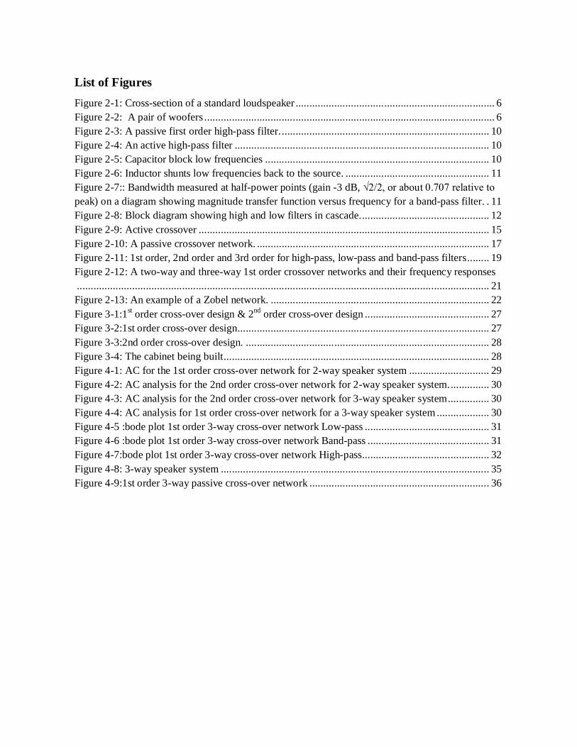
List of Figures Figure 2-1: Cross-section of a standard loudspeaker ........................................................................ 6

Figure 2-2: A pair of woofers ......................................................................................................... 6

Figure 2-3: A passive first order high-pass filter. ........................................................................... 10

Figure 2-4: An active high-pass filter ............................................................................................ 10

Figure 2-5: Capacitor block low frequencies ................................................................................. 10

Figure 2-6: Inductor shunts low frequencies back to the source. .................................................... 11

Figure 2-7:: Bandwidth measured at half-power points (gain -3 dB, √2/2, or about 0.707 relative to peak) on a diagram showing magnitude transfer function versus frequency for a band-pass filter. . 11

Figure 2-8: Block diagram showing high and low filters in cascade. .............................................. 12

Figure 2-9: Active crossover ......................................................................................................... 15

Figure 2-10: A passive crossover network. .................................................................................... 17

Figure 2-11: 1st order, 2nd order and 3rd order for high-pass, low-pass and band-pass filters ........ 19

Figure 2-12: A two-way and three-way 1st order crossover networks and their frequency responses ..................................................................................................................................................... 21

Figure 2-13: An example of a Zobel network. ............................................................................... 22

Figure 3-1:1st order cross-over design & 2nd order cross-over design ............................................. 27

Figure 3-2:1st order cross-over design ........................................................................................... 27

Figure 3-3:2nd order cross-over design. ........................................................................................ 28

Figure 3-4: The cabinet being built ................................................................................................ 28

Figure 4-1: AC for the 1st order cross-over network for 2-way speaker system ............................. 29

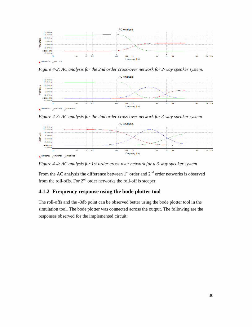
Figure 4-2: AC analysis for the 2nd order cross-over network for 2-way speaker system. .............. 30

Figure 4-3: AC analysis for the 2nd order cross-over network for 3-way speaker system ............... 30

Figure 4-4: AC analysis for 1st order cross-over network for a 3-way speaker system ................... 30

Figure 4-5 :bode plot 1st order 3-way cross-over network Low-pass ............................................. 31

Figure 4-6 :bode plot 1st order 3-way cross-over network Band-pass ............................................ 31

Figure 4-7:bode plot 1st order 3-way cross-over network High-pass.............................................. 32

Figure 4-8: 3-way speaker system ................................................................................................. 35

Figure 4-9:1st order 3-way passive cross-over network ................................................................. 36

List of Tables

Table 1: Comparison of calculated values to simulated values ....................................................... 32

Table 2:Compares theoretical powers and practical powers. .......................................................... 33

Table 3: Examples of Speaker wattages for 1st order 2-way cross-over network............................ 34

Table 4: Example of speaker wattages for 2nd order 3-way cross-over network ............................ 34

Table 5:Example of speaker wattages for 2nd order 2-way cross-over network ............................. 34

1

ABSTRACT Most public service vehicles and even personal cars have music systems installed with

loudspeakers but most of them produce very poor sound quality. This is because you may

find a speaker playing sound ranges which is not designed for thereby overworking the

speaker hence producing low quality sound. Crossover networks come in handy making

loudspeakers produce better sound quality. Modern multi-drive music systems on the

other hand are very expensive not many people can afford them. This is due to the

complexity of the construction and the sophisticated components used. One of the

components being crossover networks which make the system very complicated and

expensive in terms of design and manufacture. This also increases cost of repair and

maintenance of the system. Hence this cost can be reduced by using passive crossover

networks which are simple, cheaper and efficient. Choice of the speaker is also paramount

in that a speaker is chosen in terms of the power ratings, which will also dictate its size, to

fit the specifications of the music system.

2

CHAPTER 1

1. INTRODUCTION At ordinary sound pressure levels (SPL), most humans can hear down to about 20 Hz and up

to 20 KHz[1]. Speakers are chosen to handle frequencies within these limits. In two-way

loudspeaker systems, a woofer and a tweeter are employed. A three-way loudspeaker system

employs a woofer, a mid-range, and a tweeter[2]. A crossover network is incorporated to split

the audio signal into separate frequency bands that can be separately routed to loudspeakers

optimized for those bands[2]. There are two types of crossover networks which are:

1. Passive crossover networks.

2. Active crossover networks.

In a multi-drive speaker system, each driver is chosen such that it can work well with the

other drivers without either being damaged or overworked. Crossover networks are

employed since they can be used to determine the speaker power needed since the give a

relationship between power of the audio signal and its frequency which in turn determines the

speaker power handling. In order to fully understand this, there is a need to start from the

basics and understand sound as a wave and how its frequency affects its energy which

corresponds to its amplitude and how to correlate this concept with the working principle of

the speaker.

1.1 Problem Definition

To come up with a power selection method for speaker drives for a passive crossover network. Reasons for this are:

To reduce the cost of constructing multi-drive music systems.

To reduce power wastage by speaker drives in music systems.

The most common method used for power selection of speaker drives is by using the amplifier power rating to determine the speaker drives to be used which might cause inaccuracy in the exact power needed hence having a huge impact on cost and also power wastage.

Thus, the aim of the project is to come up with an accurate power selection method for speaker drives for a passive crossover network so as to cut down on cost and also power

3

wastage in a nutshell.

1.2 Objectives

The objective of the project is to come up with a power selection method for a passive crossover network, specifically for a two-way speaker system and a three-way speaker system for:

First-order passive filter.

Second-order passive filter.

CHAPTER 2

2 LITERATURE REVIEW

2.1 Sound

Sound is a vibration that propagates as a mechanical wave of pressure and displacement, through some medium (such as air or water). Sometimes sound refers to only those vibrations with frequencies that are within the range of hearing for humans or for a particular animal.

2.1.1 Propagation of sound Sound propagates through compressible media such as air, water and solids as longitudinal waves and also as a transverse waves in solids. The sound waves are generated by a sound source, such as the vibrating diaphragm of a stereo speaker. The sound source creates vibrations in the surrounding medium. As the source continues to vibrate the medium, the vibrations propagate away from the source at the speed of sound, thus forming the sound wave. At a fixed distance from the source, the pressure, velocity, and displacement of the medium vary in time. At an instant in time, the pressure, velocity, and displacement vary in space. Note that the particles of the medium do not travel with the sound wave.

This is intuitively obvious for a solid, and the same is true for liquids and gases (that is, the vibrations of particles in the gas or liquid transport the vibrations, while the average position of the particles over time does not change). During propagation, waves can be reflected, refracted, or attenuated by the medium.

The behavior of sound propagation is generally affected by three things:

A relationship between density and pressure. This relationship, affected by temperature, determines the speed of sound within the medium.

The propagation is also affected by the motion of the medium itself. For example, sound moving through wind. Independent of the motion of sound through the medium, if the medium is moving, the sound is further transported.

4

The viscosity of the medium also affects the motion of sound waves. It determines the rate at which sound is attenuated. For many media, such as air or water, attenuation due to viscosity is negligible.

When sound is moving through a medium that does not have constant physical properties, it may be refracted (either dispersed or focused).

The mechanical vibrations that can be interpreted as sound are able to travel through all forms of matter: gases, liquids, solids, and plasmas. The matter that supports the sound is called the medium. Sound cannot travel through a vacuum[3].

2.1.1.1 Sound wave characteristic and properties Sound waves are often simplified to a description in terms of sinusoidal plane waves, which are characterized by these generic properties:

Frequency, or its inverse, the period Wavelength Wave number Amplitude Sound pressure Sound intensity Speed of sound Direction

2.1.1.2 Frequency and Amplitude An audio frequency (abbreviation: AF) or audible frequency is characterized as a periodic vibration whose frequency is audible to the average human. It is the property of sound that most determines pitch and is measured in hertz (Hz)[3].

The generally accepted standard range of audible frequencies is 20 to 20,000 Hz, although the range of frequencies individuals hear is greatly influenced by environmental factors. Frequencies below 20 Hz are generally felt rather than heard, assuming the amplitude of the vibration is great enough. Frequencies above 20,000 Hz can sometimes be sensed by young people. High frequencies are the first to be affected by hearing loss due to age and/or prolonged exposure to very loud noises[1]. The amplitude of a sound wave is specified in terms of pressure hence a logarithmic dB amplitude scale used. The quietest sound that humans can hear has amplitude of 20µPa or a sound pressure level of 0dB. Sound pressure

5

level (SPL) is the local pressure deviation from ambient atmospheric pressure caused by a sound wave measured in Pascal[4].

2.2 Working principle of a speaker

Technically we can define speaker, as a component which converts the electrical signals into the equivalent air vibrations to make audible sound. To understand the working of a speaker, we first need to understand the concept of sound. A sound is nothing but vibrations in air particles. When a sound source generates a sound, it generally makes a vibration in its surrounding air particles which finally reaches to our eardrum. Sound is characterized by the parameters like frequency, speed, fluctuation, pressure, etc. The speaker works on the same concept. It produces vibrations in air particles in order to generate a sound [2].

2.2.1 Loudspeakers

A loudspeaker (or "speaker", or in the early days of radio "loud-speaker") is an electro acoustic transducer that produces sound in response to an electrical audio signal input. In other words, speakers convert electrical signals into audible signals.

The term "loudspeaker" may refer to individual transducers (known as "drivers") or to complete speaker systems consisting of an enclosure including one or more drivers. To adequately reproduce a wide range of frequencies, most loudspeaker systems employ more than one driver, particularly for higher sound pressure level or maximum accuracy. Individual drivers are used to reproduce different frequency ranges. The drivers are named subwoofers (for very low frequencies); woofers (low frequencies); mid-range speakers (middle frequencies); tweeters (high frequencies); and sometimes super tweeters, optimized for the highest audible frequencies. The terms for different speaker drivers differ, depending on the application. In two-way systems there is no mid-range driver, so the task of reproducing the mid-range sounds falls upon the woofer and tweeter. When multiple drivers are used in a system, a "filter network", called a crossover, separates the incoming signal into different frequency ranges and routes them to the appropriate driver. A loudspeaker system with n separate frequency bands is described as "n-way speakers": a two-way system will have a woofer and a tweeter; a three-way system employs a woofer, a mid-range, and a tweeter. Loudspeakers were described as "dynamic" to distinguish them from the earlier moving iron speaker, or speakers using piezoelectric or electrostatic systems as opposed to a voice coil that moves through a steady magnetic field[2].

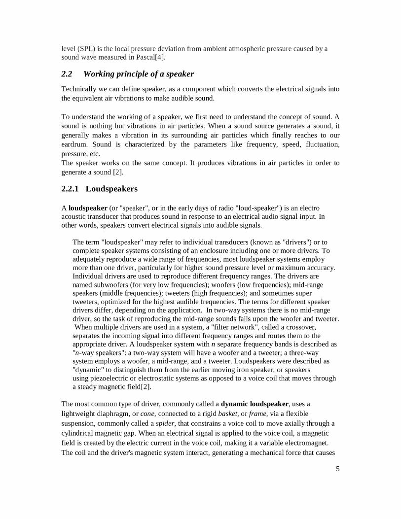
The most common type of driver, commonly called a dynamic loudspeaker, uses a lightweight diaphragm, or cone, connected to a rigid basket, or frame, via a flexible suspension, commonly called a spider, that constrains a voice coil to move axially through a cylindrical magnetic gap. When an electrical signal is applied to the voice coil, a magnetic field is created by the electric current in the voice coil, making it a variable electromagnet. The coil and the driver's magnetic system interact, generating a mechanical force that causes

6

the coil (and thus, the attached cone) to move back and forth, thereby reproducing sound under the control of the applied electrical signal coming from the amplifier.

Figure 2-1: Cross-section of a standard loudspeaker

2.2.1.1.1 Woofer A woofer is a driver that reproduces low frequencies. The driver combines with the enclosure design to produce suitable low frequencies. Some loudspeaker systems use a woofer for the lowest frequencies, sometimes well enough that a subwoofer is not needed. Additionally, some loudspeakers use the woofer to handle middle frequencies, eliminating the mid-range driver. This can be accomplished with the selection of a tweeter that can work low enough that, combined with a woofer that responds high enough, the two drivers add coherently in the middle frequencies. It is commonly used to produce low frequency sounds, typically from around 40 hertz up to about a kilohertz or higher. The most common design for a woofer is the electrodynamics’ driver, which typically uses a stiff paper cone, driven by a voice coil which is surrounded by a magnetic field.

Figure 2-2: A pair of woofers

2.2.1.1.2 Mid-Range A mid-range speaker is a loudspeaker driver that reproduces middle frequencies. Mid-range driver diaphragms can be made of paper or composite materials, and can be direct radiation drivers (rather like smaller woofers) or they can be compression drivers (rather like some tweeter designs). If the mid-range driver is a direct radiator, it can be mounted on the front baffle of a loudspeaker enclosure, or, if a compression driver, mounted at the throat of a horn for added output level and control of radiation pattern. A mid-range speaker is

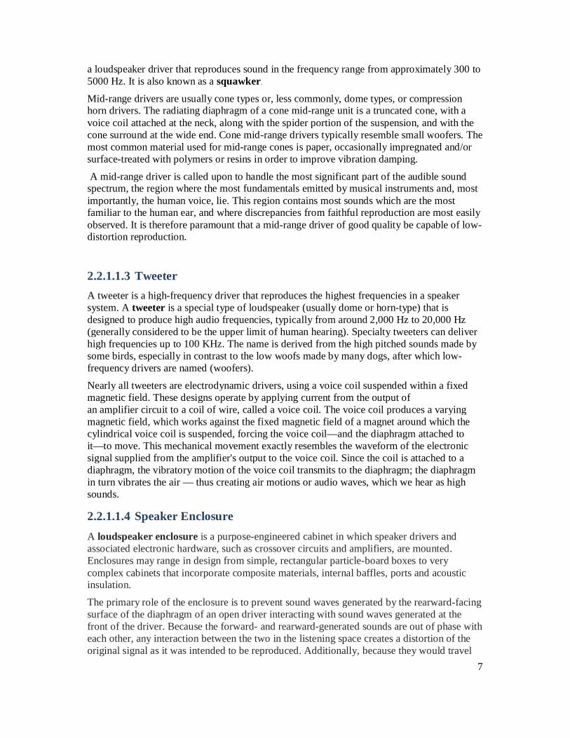
7

a loudspeaker driver that reproduces sound in the frequency range from approximately 300 to 5000 Hz. It is also known as a squawker.

Mid-range drivers are usually cone types or, less commonly, dome types, or compression horn drivers. The radiating diaphragm of a cone mid-range unit is a truncated cone, with a voice coil attached at the neck, along with the spider portion of the suspension, and with the cone surround at the wide end. Cone mid-range drivers typically resemble small woofers. The most common material used for mid-range cones is paper, occasionally impregnated and/or surface-treated with polymers or resins in order to improve vibration damping.

A mid-range driver is called upon to handle the most significant part of the audible sound spectrum, the region where the most fundamentals emitted by musical instruments and, most importantly, the human voice, lie. This region contains most sounds which are the most familiar to the human ear, and where discrepancies from faithful reproduction are most easily observed. It is therefore paramount that a mid-range driver of good quality be capable of low-distortion reproduction.

2.2.1.1.3 Tweeter A tweeter is a high-frequency driver that reproduces the highest frequencies in a speaker system. A tweeter is a special type of loudspeaker (usually dome or horn-type) that is designed to produce high audio frequencies, typically from around 2,000 Hz to 20,000 Hz (generally considered to be the upper limit of human hearing). Specialty tweeters can deliver high frequencies up to 100 KHz. The name is derived from the high pitched sounds made by some birds, especially in contrast to the low woofs made by many dogs, after which low-frequency drivers are named (woofers).

Nearly all tweeters are electrodynamic drivers, using a voice coil suspended within a fixed magnetic field. These designs operate by applying current from the output of an amplifier circuit to a coil of wire, called a voice coil. The voice coil produces a varying magnetic field, which works against the fixed magnetic field of a magnet around which the cylindrical voice coil is suspended, forcing the voice coil—and the diaphragm attached to it—to move. This mechanical movement exactly resembles the waveform of the electronic signal supplied from the amplifier's output to the voice coil. Since the coil is attached to a diaphragm, the vibratory motion of the voice coil transmits to the diaphragm; the diaphragm in turn vibrates the air — thus creating air motions or audio waves, which we hear as high sounds.

2.2.1.1.4 Speaker Enclosure A loudspeaker enclosure is a purpose-engineered cabinet in which speaker drivers and associated electronic hardware, such as crossover circuits and amplifiers, are mounted. Enclosures may range in design from simple, rectangular particle-board boxes to very complex cabinets that incorporate composite materials, internal baffles, ports and acoustic insulation.

The primary role of the enclosure is to prevent sound waves generated by the rearward-facing surface of the diaphragm of an open driver interacting with sound waves generated at the front of the driver. Because the forward- and rearward-generated sounds are out of phase with each other, any interaction between the two in the listening space creates a distortion of the original signal as it was intended to be reproduced. Additionally, because they would travel

8

different paths through the listening space, the sound waves would arrive at the listener's position at slightly different times; introducing echo and reverberation effects not part of the original sound. The enclosure also plays a role in managing vibration induced by the driver frame and moving air mass within the enclosure, as well as heat generated by driver voice coils and amplifiers (especially where woofers and subwoofers are concerned). Sometimes considered part of the enclosure, the base may include specially designed "feet" to decouple the speaker from the floor[2].

2.2.1.1.5 Relationship between speaker power, sound and frequency Why a subwoofer must have a large diameter? Why can't it have the same diameter as a tweeter? This is a very common thing that people think, it also yields statements like "you can't ever get low bass out of headphones because the drivers are so small" or that there is some kind of relationship between the diameter of the driver and the largest wavelength (lowest frequency) it can reproduce. Low-frequency drivers are large and high-frequency drivers are small. This is due to the energy carried by the sound waves. Frequency is directly proportional to energy hence, a very high-frequency wave has very high energy, and it only takes relatively little amplitude to carry a lot of energy. Low frequency waves are not very energetic due to this, and hence require very high amplitude to have the same energy. In order to be loud, you need a lot of low-frequency amplitude, and relatively little high-frequency amplitude. So high-frequency drivers don't need to displace a whole lot of air and create a lot of pressure, so they can be small. Additionally, high frequencies obviously require very fast motion, which requires a driver with very little mass[5].

Power (P) delivered by an amplifier to a loudspeaker is determined by dividing the voltage (v) squared by the impedance of the speaker (z). This voltage corresponds to amplitude of the sound wave since the electrical signal is converted to equivalent air vibration to create audible sound. i.e. P= V2/Z[6].

2.3 Filters

Electronic filters are analog circuits which perform signal processing functions, specifically to remove unwanted frequency components from the signal, to enhance wanted ones, or both[7]. Electronic filters can be:

Passive or active analog or digital High-pass, low-pass, band pass, band-reject (band reject; notch), or all-pass. discrete-time (sampled) or continuous-time linear or non-linear infinite impulse response (IIR type) or finite impulse response (FIR type)

9

The most common types of electronic filters are linear filters, regardless of other aspects of their design.

2.3.1 Classification of filters

2.3.1.1 Passive filters Passive implementations of linear filters are based on combinations of resistors (R), inductors (L) and capacitors (C). These types are collectively known as passive filters, because they do not depend upon an external power supply and/or they do not contain active components such as transistors. Inductors block high-frequency signals and conduct low-frequency signals, while capacitors do the reverse. A filter in which the signal passes through an inductor, or in which a capacitor provides a path to ground, presents less attenuation to low-frequency signals than high-frequency signals and is therefore a low-pass filter. If the signal passes through a capacitor, or has a path to ground through an inductor, then the filter presents less attenuation to high-frequency signals than low-frequency signals and therefore is a high-pass filter. Resistors on their own have no frequency-selective properties, but are added to inductors and capacitors to determine the time-constants of the circuit, and therefore the frequencies to which it responds.

The inductors and capacitors are the reactive elements of the filter. The number of elements determines the order of the filter. In this context, an LC tuned circuit being used in a band-pass or band-stop filter is considered a single element even though it consists of two components.

At high frequencies (above about 100 megahertz), sometimes the inductors consist of single loops or strips of sheet metal, and the capacitors consist of adjacent strips of metal. These inductive or capacitive pieces of metal are called stubs.

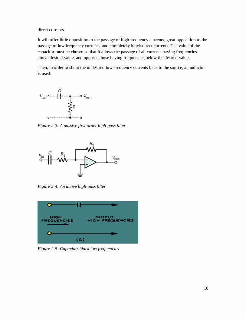
2.3.1.2 Active filters Active filters are implemented using a combination of passive and active (amplifying) components, and require an outside power source. Operational amplifiers are frequently used in active filter designs. These can have high Q factor, and can achieve resonance without the use of inductors. However, their upper frequency limit is limited by the bandwidth of the amplifiers.

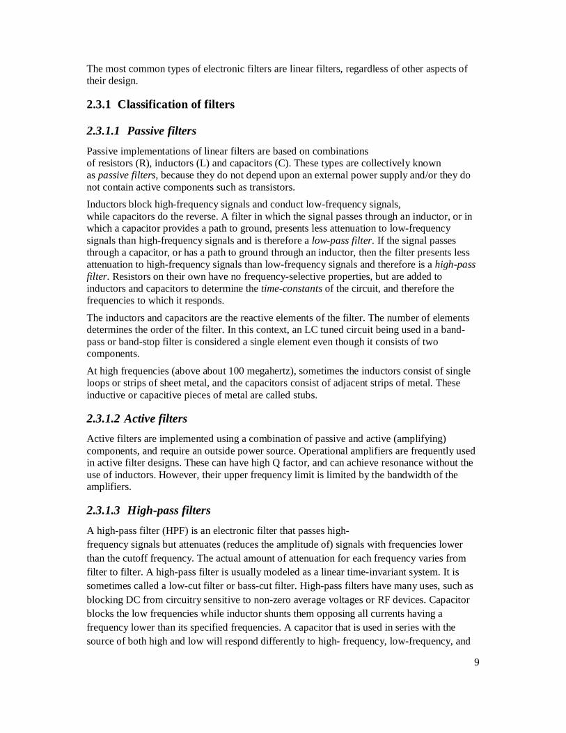
2.3.1.3 High-pass filters A high-pass filter (HPF) is an electronic filter that passes high-frequency signals but attenuates (reduces the amplitude of) signals with frequencies lower than the cutoff frequency. The actual amount of attenuation for each frequency varies from filter to filter. A high-pass filter is usually modeled as a linear time-invariant system. It is sometimes called a low-cut filter or bass-cut filter. High-pass filters have many uses, such as blocking DC from circuitry sensitive to non-zero average voltages or RF devices. Capacitor blocks the low frequencies while inductor shunts them opposing all currents having a frequency lower than its specified frequencies. A capacitor that is used in series with the source of both high and low will respond differently to high- frequency, low-frequency, and

10

direct currents.

It will offer little opposition to the passage of high frequency currents, great opposition to the passage of low frequency currents, and completely block direct currents .The value of the capacitor must be chosen so that it allows the passage of all currents having frequencies above desired value, and opposes those having frequencies below the desired value.

Then, in order to shunt the undesired low-frequency currents back to the source, an inductor is used.

Figure 2-3: A passive first order high-pass filter.

Figure 2-4: An active high-pass filter

Figure 2-5: Capacitor block low frequencies

11

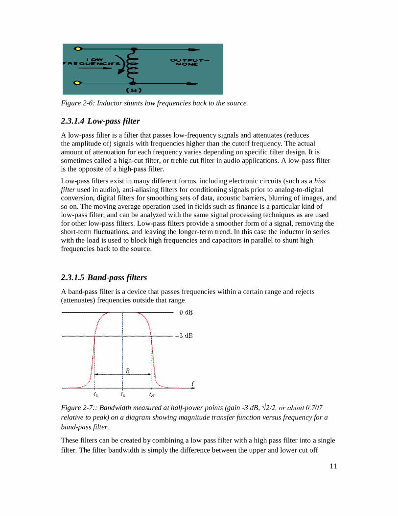
Figure 2-6: Inductor shunts low frequencies back to the source.

2.3.1.4 Low-pass filter A low-pass filter is a filter that passes low-frequency signals and attenuates (reduces the amplitude of) signals with frequencies higher than the cutoff frequency. The actual amount of attenuation for each frequency varies depending on specific filter design. It is sometimes called a high-cut filter, or treble cut filter in audio applications. A low-pass filter is the opposite of a high-pass filter. Low-pass filters exist in many different forms, including electronic circuits (such as a hiss filter used in audio), anti-aliasing filters for conditioning signals prior to analog-to-digital conversion, digital filters for smoothing sets of data, acoustic barriers, blurring of images, and so on. The moving average operation used in fields such as finance is a particular kind of low-pass filter, and can be analyzed with the same signal processing techniques as are used for other low-pass filters. Low-pass filters provide a smoother form of a signal, removing the short-term fluctuations, and leaving the longer-term trend. In this case the inductor in series with the load is used to block high frequencies and capacitors in parallel to shunt high frequencies back to the source.

2.3.1.5 Band-pass filters A band-pass filter is a device that passes frequencies within a certain range and rejects (attenuates) frequencies outside that range.

Figure 2-7:: Bandwidth measured at half-power points (gain -3 dB, √2/2, or about 0.707 relative to peak) on a diagram showing magnitude transfer function versus frequency for a band-pass filter.

These filters can be created by combining a low pass filter with a high pass filter into a single filter. The filter bandwidth is simply the difference between the upper and lower cut off

12

frequencies

Figure 2-8: Block diagram showing high and low filters in cascade.

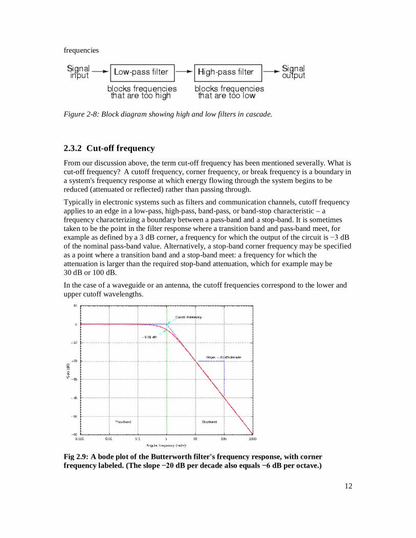
2.3.2 Cut-off frequency From our discussion above, the term cut-off frequency has been mentioned severally. What is cut-off frequency? A cutoff frequency, corner frequency, or break frequency is a boundary in a system's frequency response at which energy flowing through the system begins to be reduced (attenuated or reflected) rather than passing through.

Typically in electronic systems such as filters and communication channels, cutoff frequency applies to an edge in a low-pass, high-pass, band-pass, or band-stop characteristic – a frequency characterizing a boundary between a pass-band and a stop-band. It is sometimes taken to be the point in the filter response where a transition band and pass-band meet, for example as defined by a 3 dB corner, a frequency for which the output of the circuit is −3 dB of the nominal pass-band value. Alternatively, a stop-band corner frequency may be specified as a point where a transition band and a stop-band meet: a frequency for which the attenuation is larger than the required stop-band attenuation, which for example may be 30 dB or 100 dB. In the case of a waveguide or an antenna, the cutoff frequencies correspond to the lower and upper cutoff wavelengths.

Fig 2.9: A bode plot of the Butterworth filter's frequency response, with corner frequency labeled. (The slope −20 dB per decade also equals −6 dB per octave.)

13

Another definition is cutoff frequency or corner frequency is the frequency either above or below which the power output of a circuit, such as a line amplifier, or electronic filter has fallen to a given proportion of the power in the pass band. Most frequently this proportion is one half the pass band power, also referred to as the 3 dB point since a fall of 3 dB corresponds approximately to half power. As a voltage ratio this is a fall to of the pass band voltage[8].

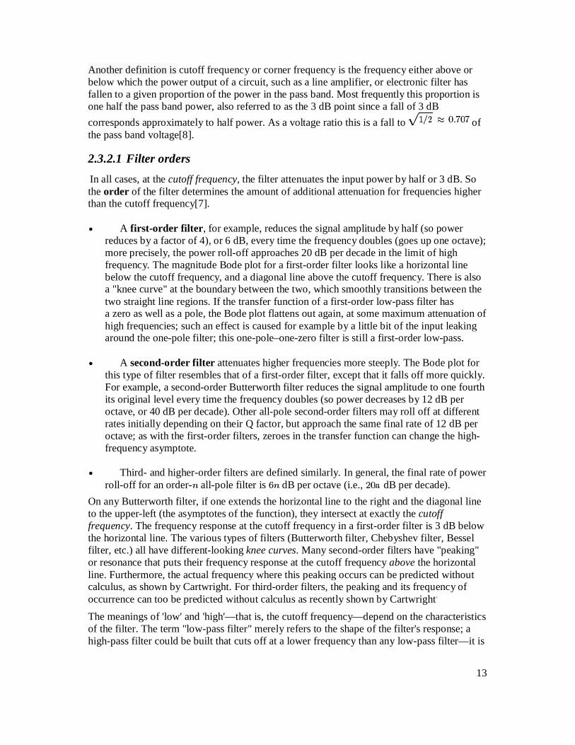
2.3.2.1 Filter orders In all cases, at the cutoff frequency, the filter attenuates the input power by half or 3 dB. So the order of the filter determines the amount of additional attenuation for frequencies higher than the cutoff frequency[7].

A first-order filter, for example, reduces the signal amplitude by half (so power reduces by a factor of 4), or 6 dB, every time the frequency doubles (goes up one octave); more precisely, the power roll-off approaches 20 dB per decade in the limit of high frequency. The magnitude Bode plot for a first-order filter looks like a horizontal line below the cutoff frequency, and a diagonal line above the cutoff frequency. There is also a "knee curve" at the boundary between the two, which smoothly transitions between the two straight line regions. If the transfer function of a first-order low-pass filter has a zero as well as a pole, the Bode plot flattens out again, at some maximum attenuation of high frequencies; such an effect is caused for example by a little bit of the input leaking around the one-pole filter; this one-pole–one-zero filter is still a first-order low-pass.

A second-order filter attenuates higher frequencies more steeply. The Bode plot for this type of filter resembles that of a first-order filter, except that it falls off more quickly. For example, a second-order Butterworth filter reduces the signal amplitude to one fourth its original level every time the frequency doubles (so power decreases by 12 dB per octave, or 40 dB per decade). Other all-pole second-order filters may roll off at different rates initially depending on their Q factor, but approach the same final rate of 12 dB per octave; as with the first-order filters, zeroes in the transfer function can change the high-frequency asymptote.

Third- and higher-order filters are defined similarly. In general, the final rate of power roll-off for an order- all-pole filter is dB per octave (i.e., dB per decade).

On any Butterworth filter, if one extends the horizontal line to the right and the diagonal line to the upper-left (the asymptotes of the function), they intersect at exactly the cutoff frequency. The frequency response at the cutoff frequency in a first-order filter is 3 dB below the horizontal line. The various types of filters (Butterworth filter, Chebyshev filter, Bessel filter, etc.) all have different-looking knee curves. Many second-order filters have "peaking" or resonance that puts their frequency response at the cutoff frequency above the horizontal line. Furthermore, the actual frequency where this peaking occurs can be predicted without calculus, as shown by Cartwright. For third-order filters, the peaking and its frequency of occurrence can too be predicted without calculus as recently shown by Cartwright. The meanings of 'low' and 'high'—that is, the cutoff frequency—depend on the characteristics of the filter. The term "low-pass filter" merely refers to the shape of the filter's response; a high-pass filter could be built that cuts off at a lower frequency than any low-pass filter—it is

14

their responses that set them apart. Electronic circuits can be devised for any desired frequency range, right up through microwave frequencies (above 1 GHz) and higher.

What do we mean by 6dB per octave? In electronics, an octave is a doubling or halving of a frequency[7]. Along with the decade, it is a unit used to describe frequency bands or frequency ratios. A frequency ratio expressed in octaves is the base-2 logarithm (binary logarithm) of the ratio:

An amplifier or filter may be stated to have a frequency response of ±6dB per octave over a particular frequency range, which signifies that the power gain changes by ±6 decibels (a factor of 4 in power), when the frequency changes by a factor of 2. This slope, or more precisely decibels per octave, corresponds to an amplitude gain proportional to frequency, which is equivalent to ±20dB per decade (factor of 10 amplitude gain change for a factor of 10 frequency change). This would be a first-order filter.

2.4 Audio crossover

Audio crossovers are a class of electronic filter used in audio applications. Most individual loudspeaker drivers are incapable of covering the entire audio spectrum from low frequencies to high frequencies with acceptable relative volume and absence of distortion so most hi-fi speaker systems use a combination of multiple loudspeakers drivers, each catering for a different frequency band. Crossovers split the audio signal into separate frequency bands that can be separately routed to loudspeakers optimized for those bands.

The need for a crossover can be attributed to the inability of most drivers to reproduce the entire musical spectrum smoothly and efficiently hence because of this most speaker systems are comprised of several drivers each of which is dedicated to the reproduction of a specific range of frequencies.

These frequencies are routed to the appropriate driver by a crossover network. This audio device divides frequencies into two or more frequency bands. A crossover network also prevents potentially damaging low frequency energy (woofer) from reaching the midrange or tweeter[9].

There are two types of audio crossovers based on their location in the audio signal path:

Active crossover.

Passive crossover

15

2.4.1 Active crossover Active crossovers are distinguished from passive crossovers in that they divide the audio signal prior to amplification. Active crossovers come in both digital and analog varieties. Digital active crossovers often include additional signal processing, such as limiting, delay, and equalization. An active crossover contains active components (i.e., those with gain) in its filters. In recent years, the most commonly used active device is an op-amp; active crossovers are operated at levels suited to power amplifier inputs in contrast to passive crossovers which operate after the power amplifier's output, at high current and in some cases high voltage. On the other hand, all circuits with gain introduce noise, and such noise has a deleterious effect when introduced prior to the signal being amplified by the power amplifiers.

Figure 2-9: Active crossover

Active crossovers always require the use of power amplifiers for each output band. Thus a 2-way active crossover needs two amplifiers—one each for the woofer and tweeter. This means that an active crossover based system will often cost more than a passive crossover based system. Despite the cost and complication disadvantages, active crossovers provide the following advantages over passive ones:

A frequency response independent of the dynamic changes in a driver's electrical characteristics.

Typically, the possibility of an easy way to vary or fine tune each frequency band to the specific drivers used. Examples would be crossover slope, filter type (e.g., Bessel, Butterworth, etc.), relative levels, ...

Better isolation of each driver from signals handled by other drivers, thus reducing intermodulation distortion and overdriving.

The power amplifiers are directly connected to the speaker drivers, thereby maximizing amplifier damping control of the speaker voice coil, reducing consequences of dynamic changes in driver electrical characteristics, all of which are likely to improve the transient response of the system.

Reduction in power amplifier output requirement. With no energy being lost in passive components, amplifier requirements are reduced considerably (up to 1/2 in some cases), reducing costs, and potentially increasing quality.

16

2.4.1.1 Advantages and disadvantages of Active Crossover

2.4.1.1.1 Advantages They lack inductors, thereby reducing the problems associated with those

components. The op amp-based active filter can achieve very good accuracy, provided that low-

tolerance resistors and capacitors are used. They can easily be made tunable; that is, controls can be added to vary the cut off

frequency which is a very useful facility in difficult communication situations where only the minimum bandwidth for intelligible communication is required. A relatively recent development in the control of the response of active filters involves the switching capacitors and resistors at high frequency, varying the effective values of these components.

The active filter crossover components will not change to the short term due to internal heating.

They are cheap since they have no inductors which are very expensive.

2.4.1.1.2 Disadvantages Active filters generate noise due to their amplifying circuitry. High power consumption unlike passive filters.

2.4.2 Passive crossover A passive crossover is different from active crossover since its location in the audio signal path is after the amplifier i.e. between the amplifier and the drivers and it is also made entirely of passive components, arranged most commonly in a Cauer topology to achieve a Butterworth filter. Passive filters use resistors combined with reactive components such as capacitors and inductors. Very high performance passive crossovers are likely to be more expensive than active crossovers since individual components capable of good performance at the high currents and voltages at which speaker systems are driven are hard to make. Polypropylene, metalized polyester foil, paper and electrolytic capacitors are common. Inductors may have air cores, powdered metal cores, ferrite cores, or laminated silicon steel cores, and most are wound with enameled copper wire. Some passive networks include devices such as fuses, PTC devices, bulbs or circuit breakers to protect the loudspeaker drivers from accidental overpowering. Modern passive crossovers increasingly incorporate equalization networks (e.g., Zobel networks) that compensate for the changes in impedance with frequency inherent in virtually all loudspeakers. The issue is complex, as part of the change in impedance is due to acoustic loading changes across a driver's pass-band. On the negative side, passive networks may be bulky and cause power loss. They are not only frequency specific, but also impedance specific. This prevents interchangeability with speaker systems of different impedances. Ideal crossover filters, including impedance compensation and equalization networks, can be very difficult to design, as the components interact in complex ways. Crossover design expert Siegfried Linkwitz said of them that "the only excuse for passive crossovers is their low cost. Their behavior changes with the signal

17

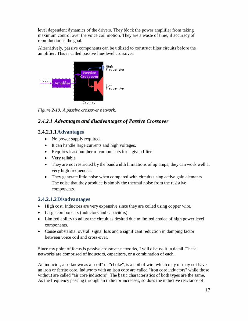
level dependent dynamics of the drivers. They block the power amplifier from taking maximum control over the voice coil motion. They are a waste of time, if accuracy of reproduction is the goal. Alternatively, passive components can be utilized to construct filter circuits before the amplifier. This is called passive line-level crossover.

Figure 2-10: A passive crossover network.

2.4.2.1 Advantages and disadvantages of Passive Crossover

2.4.2.1.1 Advantages No power supply required. It can handle large currents and high voltages. Requires least number of components for a given filter Very reliable They are not restricted by the bandwidth limitations of op amps; they can work well at

very high frequencies. They generate little noise when compared with circuits using active gain elements.

The noise that they produce is simply the thermal noise from the resistive components.

2.4.2.1.2 Disadvantages High cost. Inductors are very expensive since they are coiled using copper wire. Large components (inductors and capacitors). Limited ability to adjust the circuit as desired due to limited choice of high power level

components. Cause substantial overall signal loss and a significant reduction in damping factor

between voice coil and cross-over.

Since my point of focus is passive crossover networks, I will discuss it in detail. These networks are comprised of inductors, capacitors, or a combination of each.

An inductor, also known as a "coil" or "choke", is a coil of wire which may or may not have an iron or ferrite core. Inductors with an iron core are called "iron core inductors" while those without are called "air core inductors". The basic characteristics of both types are the same. As the frequency passing through an inductor increases, so does the inductive reactance of

18

the coil. This rise in impedance at higher frequencies allows us to use the inductor as a filter that passes low frequencies but chokes off high ones.

Capacitors do just the opposite. As frequency decreases, the capacitors reactance increases. That is, capacitors pass high frequencies and filter out low ones. These capacitors are generally non-polarized electrolytics, polypropylene, or Mylar and consist of interleaved layers of foil and insulating material.

One common myth pertaining to passive crossovers is that they "soak up" the power that is not used for each particular driver. While there is some insertion loss, the filtering action actually takes place due to the impedance mismatch created by the network.

2.4.3 Classification based on filter order or slope Just as filters have different orders, so do crossovers, depending on the filter slope they implement[8]. The final acoustic slope may be completely determined by the electrical filter or may be achieved by combining the electrical filter's slope with the natural characteristics of the driver. In the former case, the only requirement is that each driver has a flat response at least to the point where its signal is approximately −10dB down from the pass-band. In the latter case, the final acoustic slope is usually steeper than that of the electrical filters used. A third- or fourth-order acoustic crossover often has just a second order electrical filter. This requires that speaker drivers be well behaved a considerable way from the nominal crossover frequency, and further that the high frequency driver be able to survive a considerable input in a frequency range below its crossover point. This is difficult in actual practice. In the discussion below, the characteristics of the electrical filter order is discussed, followed by a discussion of crossovers having that acoustic slope and their advantages or disadvantages.

Most audio crossovers use first to fourth order electrical filters. Higher orders are not generally implemented in passive crossovers for loudspeakers, but are sometimes found in electronic equipment under circumstances for which their considerable cost and complexity can be justified.

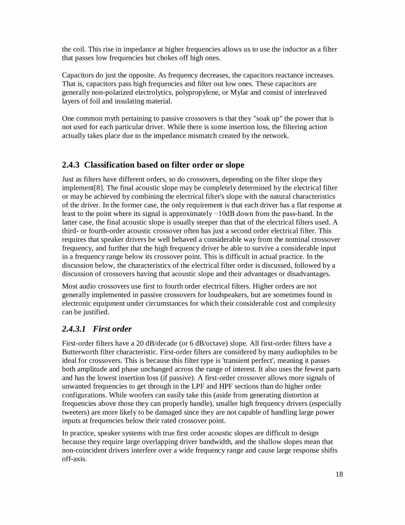
2.4.3.1 First order First-order filters have a 20 dB/decade (or 6 dB/octave) slope. All first-order filters have a Butterworth filter characteristic. First-order filters are considered by many audiophiles to be ideal for crossovers. This is because this filter type is 'transient perfect', meaning it passes both amplitude and phase unchanged across the range of interest. It also uses the fewest parts and has the lowest insertion loss (if passive). A first-order crossover allows more signals of unwanted frequencies to get through in the LPF and HPF sections than do higher order configurations. While woofers can easily take this (aside from generating distortion at frequencies above those they can properly handle), smaller high frequency drivers (especially tweeters) are more likely to be damaged since they are not capable of handling large power inputs at frequencies below their rated crossover point.

In practice, speaker systems with true first order acoustic slopes are difficult to design because they require large overlapping driver bandwidth, and the shallow slopes mean that non-coincident drivers interfere over a wide frequency range and cause large response shifts off-axis.

19

2.4.3.2 Second order Second-order filters have a 40 dB/decade (or 12 dB/octave) slope. Second-order filters can have a Bessel, Linkwitz-Riley or Butterworth characteristic depending on design choices and the components used. This order is commonly used in passive crossovers as it offers a reasonable balance between complexity, response, and higher frequency driver protection. When designed with time aligned physical placement, these crossovers have a symmetrical polar response, as do all even order crossovers. It is commonly thought that there will always be a phase difference of 180° between the outputs of a (second order) low-pass filter and a high-pass filter having the same crossover frequency. And so, in a 2-way system, the high-pass section's output is usually connected to the high frequency driver 'inverted', to correct for this phase problem. For passive systems, the tweeter is wired with opposite polarity to the woofer; for active crossovers the high-pass filter's output is inverted. In 3-way systems the mid-range driver or filter is inverted. However, this is generally only true when the speakers have a wide response overlap and the acoustic centers are physically aligned.

2.4.3.3 Third order Third-order filters have a 60 dB/decade (or 18 dB/octave) slope. These crossovers usually have Butterworth filter characteristics; phase response is very good, the level sum being flat and in phasequadratue, similar to a first order crossover. The polar response is asymmetric. In the original D'Appolito MTM arrangement, a symmetrical arrangement of drivers is used to create a symmetrical off-axis response when using third-order crossovers.

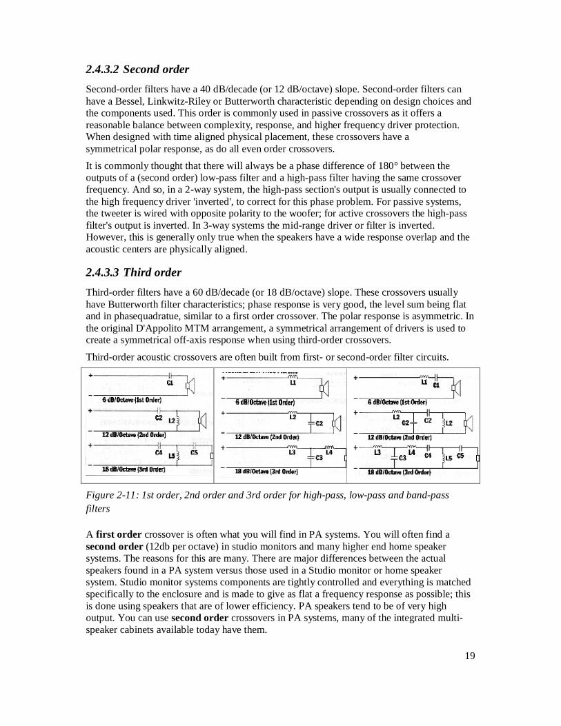
Third-order acoustic crossovers are often built from first- or second-order filter circuits.

Figure 2-11: 1st order, 2nd order and 3rd order for high-pass, low-pass and band-pass filters

A first order crossover is often what you will find in PA systems. You will often find a second order (12db per octave) in studio monitors and many higher end home speaker systems. The reasons for this are many. There are major differences between the actual speakers found in a PA system versus those used in a Studio monitor or home speaker system. Studio monitor systems components are tightly controlled and everything is matched specifically to the enclosure and is made to give as flat a frequency response as possible; this is done using speakers that are of lower efficiency. PA speakers tend to be of very high output. You can use second order crossovers in PA systems, many of the integrated multi-speaker cabinets available today have them.

20

2.4.4 Theory of Operation of a Passive Crossover Network If we place a capacitor in series with a 4 ohm tweeter, we have created a first order (6 dB/octave) high pass filter. As frequency goes down, the capacitive reactance of the capacitor goes up. At the crossover point, the impedance presented by the capacitor will be equal to the impedance of the tweeter. Since the capacitor is in series with the tweeter, the effective load impedance "seen" by the amplifier is 4 + 4 or 8 ohms. This rise in load impedance causes a 3 dB reduction in output power at the amplifier. As the frequency continues to go down, the effective impedance of the network continues to rise and the output of the amplifier continues to be reduced at a rate determined by the slope of the crossover. In our example, the roll-off rate would occur at 6 dB/octave because it is a first order network.

The number of inductors and capacitors in a network determines its order. For example, if a network consisted of one component it would be a first order network. Two components would comprise a second order network and so on. Final response roll off rates occur in multiples of 6 dB/octave, according to the order of the filter. Consequently, a first order network would have a slope of 6 dB/octave; a second order network would have a slope of 12 dB/octave; and so on.

It is generally accepted that 1st order networks should only be used for low-pass filters because a 6 dB/octave roll off rate will not provide adequate protection for midrange and tweeter drivers. On the other hand, slopes greater than 18 dB/octave tend to suffer from poor transient response, audible ringing, phase disparity among the drivers, and excessive insertion loss.

Insertion loss is a term used to account for the power that is lost when a passive crossover network is used. The most significant power loss occurs in the inductor due to the resistance of the wire. Some inductors can have dc resistances as high as 1 ohm. This can rob almost 20 percent of the power intended for the drivers. Although this may seem high, 20 percent is only about a 1 dB drop in output level.

Resistance in the crossover network also degrades the damping ability of the amplifier. Since the damping factor is the ratio of the load impedance to the output impedance of the amplifier, adding any resistance to the output impedance of the amp will greatly reduce the ability of the amp to control cone movement. The result of this could be bass that lacks definition or sounds muddy.

In order to reduce these problems, you must be very careful when selecting the components for your passive crossover network. The best sounding (and most expensive) capacitors are the Mylar and polypropylene high-voltage variety. These should always be used for high-pass filters because they are series components.

For low-pass filters, any type of capacitor can be used; however, the choice of inductor is more critical since it is the series element. Air core inductors are better sounding because of their lower distortion figures; unfortunately, they tend to have a higher dc resistance than iron core varieties.

21

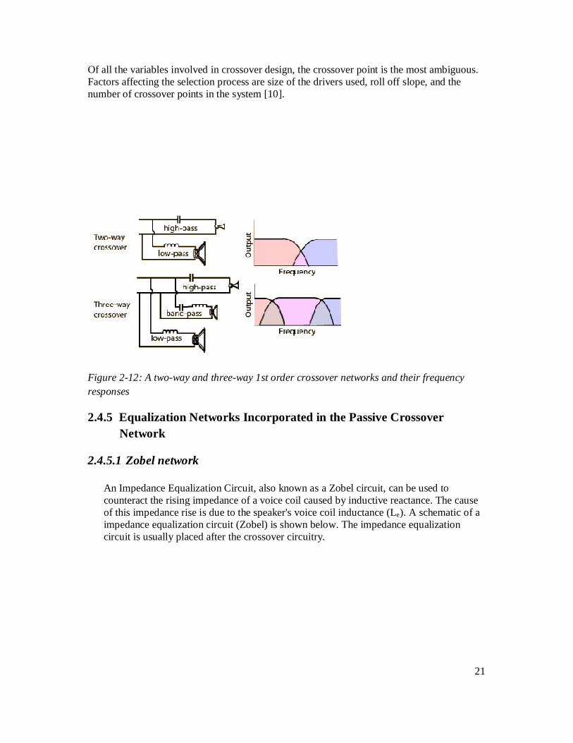
Of all the variables involved in crossover design, the crossover point is the most ambiguous. Factors affecting the selection process are size of the drivers used, roll off slope, and the number of crossover points in the system [10].

Figure 2-12: A two-way and three-way 1st order crossover networks and their frequency responses

2.4.5 Equalization Networks Incorporated in the Passive Crossover Network

2.4.5.1 Zobel network

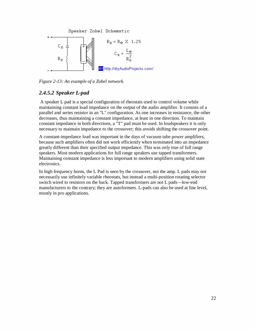
An Impedance Equalization Circuit, also known as a Zobel circuit, can be used to counteract the rising impedance of a voice coil caused by inductive reactance. The cause of this impedance rise is due to the speaker's voice coil inductance (Le). A schematic of a impedance equalization circuit (Zobel) is shown below. The impedance equalization circuit is usually placed after the crossover circuitry.

22

Figure 2-13: An example of a Zobel network.

2.4.5.2 Speaker L-pad A speaker L pad is a special configuration of rheostats used to control volume while maintaining constant load impedance on the output of the audio amplifier. It consists of a parallel and series resistor in an "L" configuration. As one increases in resistance, the other decreases, thus maintaining a constant impedance, at least in one direction. To maintain constant impedance in both directions, a "T" pad must be used. In loudspeakers it is only necessary to maintain impedance to the crossover; this avoids shifting the crossover point. A constant-impedance load was important in the days of vacuum tube power amplifiers, because such amplifiers often did not work efficiently when terminated into an impedance greatly different than their specified output impedance. This was only true of full range speakers. Most modern applications for full range speakers use tapped transformers. Maintaining constant impedance is less important to modern amplifiers using solid state electronics. In high frequency horns, the L Pad is seen by the crossover, not the amp. L pads may not necessarily use infinitely variable rheostats, but instead a multi-position rotating selector switch wired to resistors on the back. Tapped transformers are not L pads—low-end manufacturers to the contrary; they are autoformers. L-pads can also be used at line level, mostly in pro applications.

23

CHAPTER 3

3 DESIGN

3.1 Stage 1: Design of a 1st order and 2nd order crossover networks for 2-way and 3-way speaker system

In this stage of the project research was done and from the theory learnt I was able to come up with designs for 1st order passive cross-over networks for 2-way speaker system and 3-way speaker system and also 2nd order passive cross-over networks for a 2-way and 3-way speaker systems. For example for a 2-way speaker system I designed cross-over networks that split the audio frequency into two bands of frequency, which was the same case as for a 3-way speaker where the audio frequency was split into three bands of frequency. Choice of the cross-over point is paramount for the design of cross-over networks.

3.1.1 Choosing of the crossover point

First of all the speaker impedances were chosen to be:

Woofer- 4Ω

Mid-range-8Ω

Tweeter-8Ω

For 1st order cross-over networks:

2-way speaker system: first cross-over point (fc1) = 904.29Hz

3-way speaker system: first cross-over point (fc1) = 1.026 KHz and second cross-over point (fc2) = 6.8 KHz. Band-pass FH=5.79KHz, FL=1.2KHz.

For 2nd order cross-over networks:

2-way speaker system: first cross-over point (fc1) = 1 KHz

3-way speaker system: first cross-over point (fc1) = 1 KHz and second cross-over

24

point (fc2) = 6.4 KHz. Band-pass FH=5.6KHz, FL=1KHz

3.1.2 Inductor and capacitor values

From the theory learned, values of inductors and capacitors in the cross-over networks are calculated from the formulas indicated below: (capacitor values were calculated on the basis of standard capacitors values)

Knowing the cross-over points and the speaker impedance,

1st order cross-over networks

Reactance of an inductor from first principles is given by:

XL= 2πfL from this we can get:

L=

Reactance of a capacitor from first principles is given by:

XC= from this we can get:

C= for this case, at the cross-over point the reactance is equal to the speaker

impedance= ZO.

L= and C= Where fc is the cross-over frequency.

2nd order cross-over networks the formula for finding the inductor and capacitor was found to be:

L= and C= =

3.1.2.1 2-way speaker system

3.1.2.1.1 1st order cross-over network:

Low-pass filter section

L1= = 0.7mH

High-pass filter section

C1= = 22µF

3.1.2.1.2 2nd order cross-over network.

Low-pass filter section

L2= =0.9mH

25

C2= =33µF

High-pass filter section

L1= =2.2mH

C1= =15µF

3.1.2.2 3-way speaker system

3.1.2.2.1 1st order cross-over network After much consultations and time constraints, it was decided that the 1st order cross-over network for a 3-way speaker system is to be implemented. According to the market analysis the speakers found were:

Woofer- Model JBL, 200W Peak power, 100Wrms, 4Ω

Mid-range- Model Kenwood, 260W Peak power, 40Wrms, 4Ω

Tweeter- Model Sony, 100W Peak power, 20Wrms, 5Ω

Low-pass section FC1=1.026KHz

Band-pass section FL=1.21KHz and FH=5.79KHz

High-pass section FC2=6.8KHz

Using these specifications the cross-over network was designed and values of capacitors and inductors were:

Low-pass filter section

L1=

Band-pass filter section

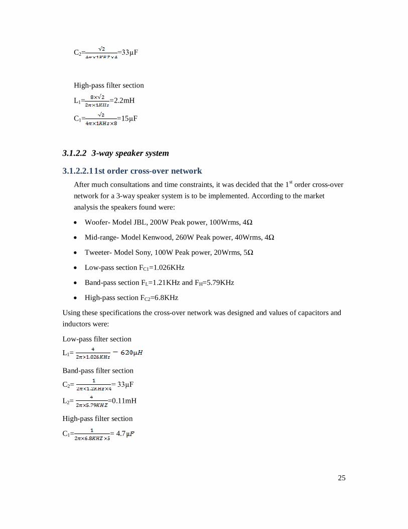
C2= = 33µF

L2= =0.11mH

High-pass filter section

C1= = 4.7

26

3.1.2.2.2 2nd order cross-over network:

Low-pass section

L2=

C2=

Band-pass section

FL=1KHZ and FL=5.6KHz

C3= =15

L3= =1.8mH

L4= =0.33mH

C4=

High-pass section

C1= =2.2µF

L1= = 275µH

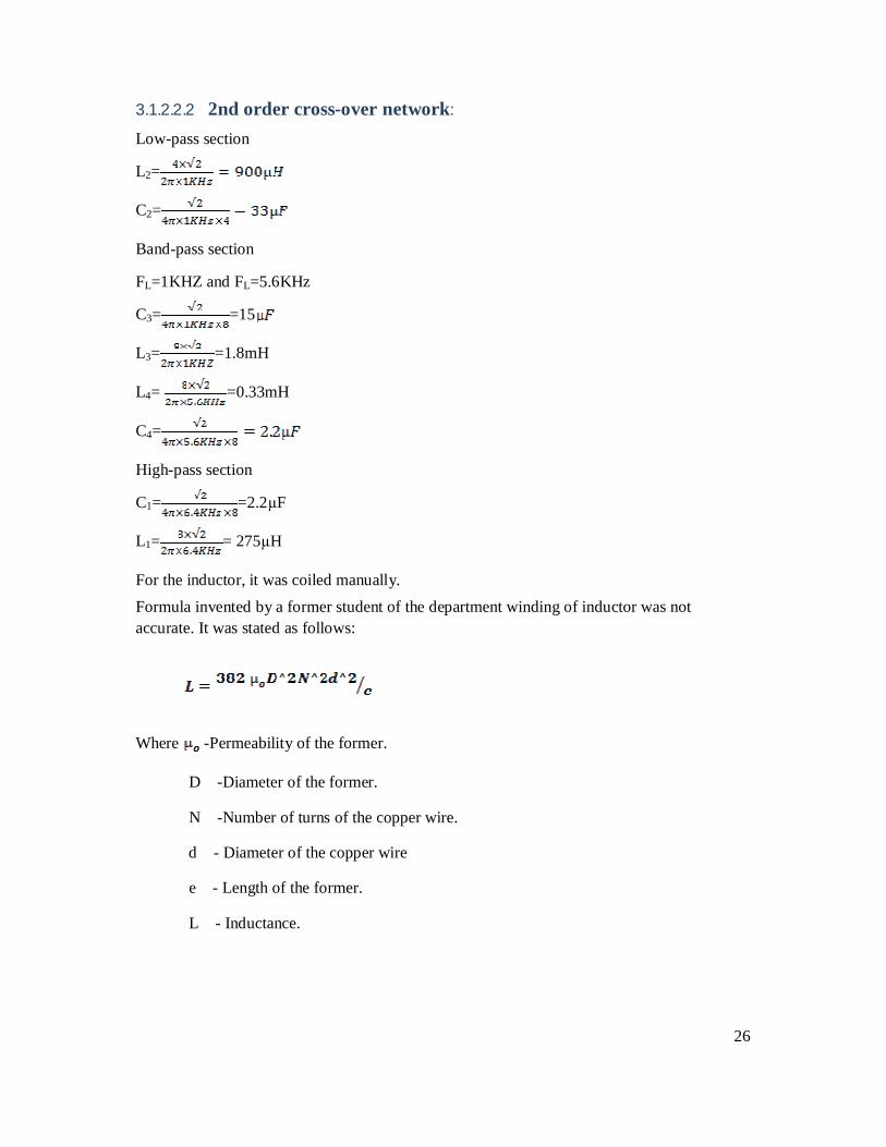
For the inductor, it was coiled manually. Formula invented by a former student of the department winding of inductor was not accurate. It was stated as follows:

Where -Permeability of the former.

D -Diameter of the former.

N -Number of turns of the copper wire.

d - Diameter of the copper wire

e - Length of the former.

L - Inductance.

27

Formula that was used research from the internet which was more accurate was:

L (µH) =31.6*N^2* r1^2 / 6*r1+ 9*l + 10*(r2-r1) where.... L( H)= Inductance in micro Henries N = Total Number of turns r1 = Radius of the inside of the coil in meters r2 = Radius of the outside of the coil in meters l = Length of the coil in meters

3.1.3 Designs

3.1.3.1 2-way cross-over networks designs

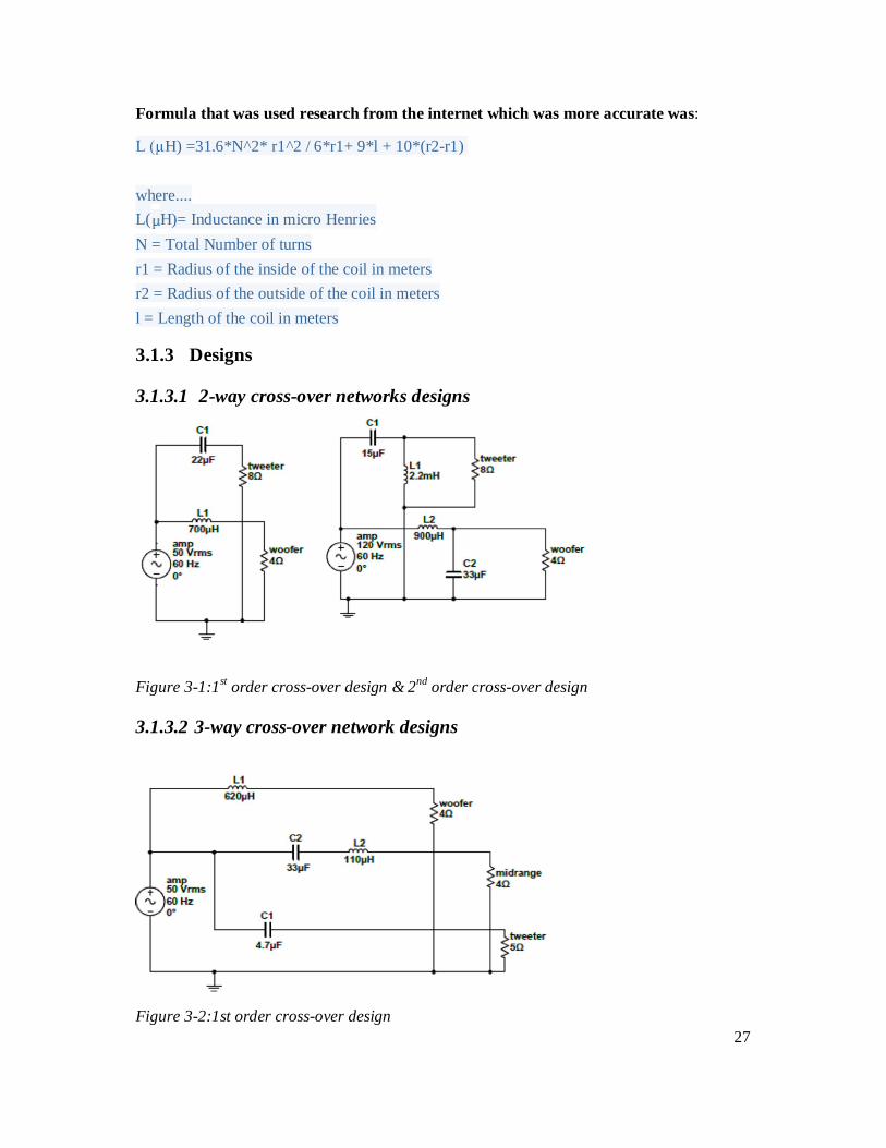
Figure 3-1:1st order cross-over design & 2nd order cross-over design

3.1.3.2 3-way cross-over network designs

Figure 3-2:1st order cross-over design

28

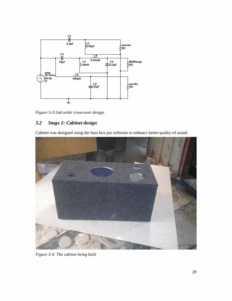
Figure 3-3:2nd order cross-over design.

3.2 Stage 2: Cabinet design

Cabinet was designed using the bass box pro software to enhance better quality of sound.

Figure 3-4: The cabinet being built

29

CHAPTER 4

4 RESULTS AND ANALYSIS

4.1 Computer simulations results

Due to the difficulty in obtaining accurate results using manual simulation, I chose to use computer simulation to do my analysis. Computer simulation enabled me to do an AC analysis of all the cross-over networks including the cross-over network that was implemented.

From the AC analysis I observed how power gain for the different drives varied with frequency. For example for woofer, power gain covered the largest area with respect to the frequency range followed by the power gain of the mid-range and then tweeter which covered the smallest area. In the literature review, it was researched that theoretically woofer wattage is more than that of the tweeter. For a multi- drive music system, energy of the sound waves from all the drives should be same so there should be a kind of a balance between the drives. For example for a woofer it compensates for its low frequency energy by having high amplitude which then corresponds to voltage of the audio signal which then means woofer will have the highest power rating.

4.1.1 AC analysis results

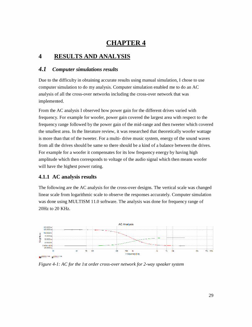
The following are the AC analysis for the cross-over designs. The vertical scale was changed linear scale from logarithmic scale to observe the responses accurately. Computer simulation was done using MULTISM 11.0 software. The analysis was done for frequency range of 20Hz to 20 KHz.

Figure 4-1: AC for the 1st order cross-over network for 2-way speaker system

30

Figure 4-2: AC analysis for the 2nd order cross-over network for 2-way speaker system.

Figure 4-3: AC analysis for the 2nd order cross-over network for 3-way speaker system

Figure 4-4: AC analysis for 1st order cross-over network for a 3-way speaker system

From the AC analysis the difference between 1st order and 2nd order networks is observed from the roll-offs. For 2nd order networks the roll-off is steeper.

4.1.2 Frequency response using the bode plotter tool

The roll-offs and the -3db point can be observed better using the bode plotter tool in the simulation tool. The bode plotter was connected across the output. The following are the responses observed for the implemented circuit:

31

4.1.2.1 1st order 3-way cross-over network

4.1.2.1.1 Low Pass Section

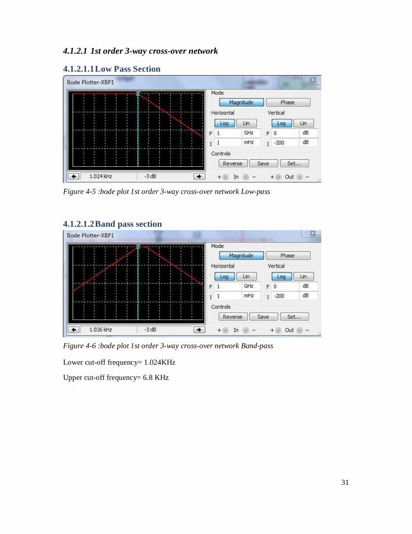
Figure 4-5 :bode plot 1st order 3-way cross-over network Low-pass

4.1.2.1.2 Band pass section

Figure 4-6 :bode plot 1st order 3-way cross-over network Band-pass

Lower cut-off frequency= 1.024KHz

Upper cut-off frequency= 6.8 KHz

32

4.1.2.1.3 High-pass section

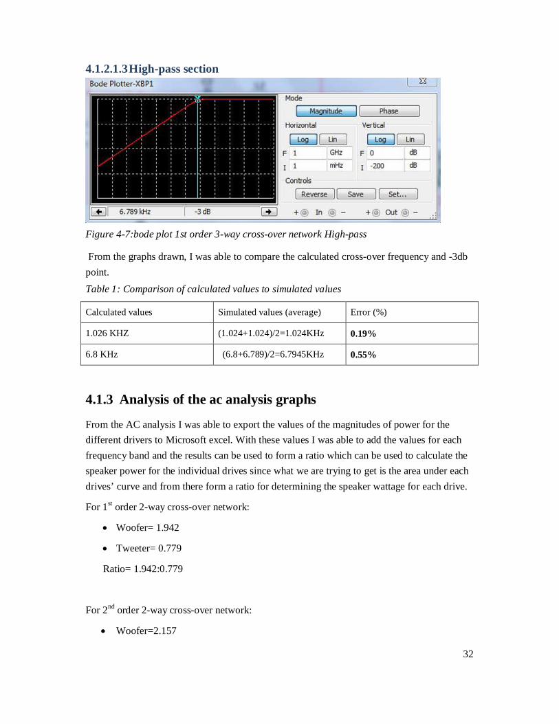
Figure 4-7:bode plot 1st order 3-way cross-over network High-pass

From the graphs drawn, I was able to compare the calculated cross-over frequency and -3db point. Table 1: Comparison of calculated values to simulated values

Calculated values Simulated values (average) Error (%)

1.026 KHZ (1.024+1.024)/2=1.024KHz 0.19%

6.8 KHz (6.8+6.789)/2=6.7945KHz 0.55%

4.1.3 Analysis of the ac analysis graphs

From the AC analysis I was able to export the values of the magnitudes of power for the different drivers to Microsoft excel. With these values I was able to add the values for each frequency band and the results can be used to form a ratio which can be used to calculate the speaker power for the individual drives since what we are trying to get is the area under each drives’ curve and from there form a ratio for determining the speaker wattage for each drive.

For 1st order 2-way cross-over network:

Woofer= 1.942

Tweeter= 0.779

Ratio= 1.942:0.779

For 2nd order 2-way cross-over network:

Woofer=2.157

33

Tweeter=0.808

Ratio= 2.157:0.808

For 2nd order 3-way cross-over network:

Woofer= 2.157

Mid-range= 0.580

Tweeter= 0.312

Ratio = 2.157:0.58:0.312

For 1st order 3-way cross-over network:

Woofer = 2.037

Mid-range= 0.917

Tweeter= 0.425

Ratio = 2.037: 0.917: 0.425

For the 1st order 3-way cross-over I was able to use the ratio above to determine the speakers I will use. I chose woofer to be 100Wrms.

Woofer= 100Wrms

Midrange= 100Wrms= 45.02Wrms

Tweeter= = 20.86Wrms

From the calculations, I was able to determine the exact speaker powers for the drives that can work well with my cross-over network.

Table 2:Compares theoretical powers and practical powers.

Drives Theoretical Wattage Practical wattage Error(%)

Woofer 100Wrms 100Wrms 0%

Mid-range 45.02Wrms 40Wrms 11.15%

Tweeter 20.86Wrms 20Wrms 4.12%

34

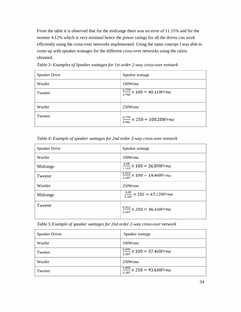
From the table it is observed that for the midrange there was an error of 11.15% and for the tweeter 4.12% which is very minimal hence the power ratings for all the drives can work efficiently using the cross-over networks implemented. Using the same concept I was able to come up with speaker wattages for the different cross-over networks using the ratios obtained. Table 3: Examples of Speaker wattages for 1st order 2-way cross-over network

Speaker Drive Speaker wattage

Woofer 100Wrms

Tweeter

Woofer 250Wrms

Tweeter

Table 4: Example of speaker wattages for 2nd order 3-way cross-over network

Speaker Drive Speaker wattage

Woofer 100Wrms

Midrange

Tweeter

Woofer 250Wrms

Midrange

Tweeter

Table 5:Example of speaker wattages for 2nd order 2-way cross-over network

Speaker Drives Speaker wattage

Woofer 100Wrms

Tweeter

Woofer 250Wrms

Tweeter

35

From the table above, speaker wattage for different cross-over networks can be chosen even if it’s not the exact wattage stated but within that range because the speaker wattages derived are not practical in the market.

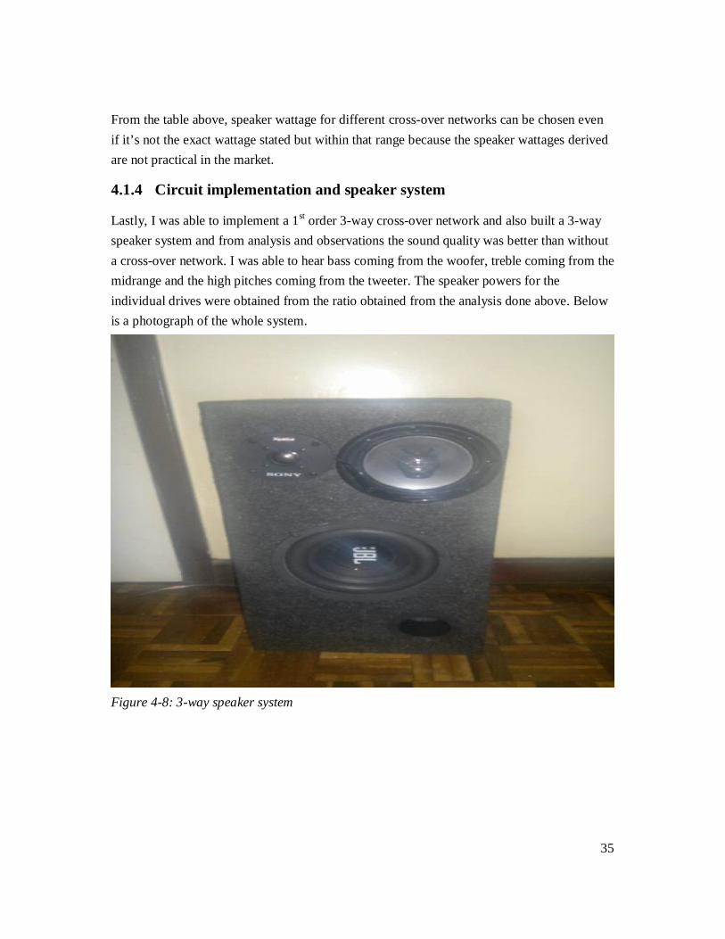
4.1.4 Circuit implementation and speaker system

Lastly, I was able to implement a 1st order 3-way cross-over network and also built a 3-way speaker system and from analysis and observations the sound quality was better than without a cross-over network. I was able to hear bass coming from the woofer, treble coming from the midrange and the high pitches coming from the tweeter. The speaker powers for the individual drives were obtained from the ratio obtained from the analysis done above. Below is a photograph of the whole system.

Figure 4-8: 3-way speaker system

36

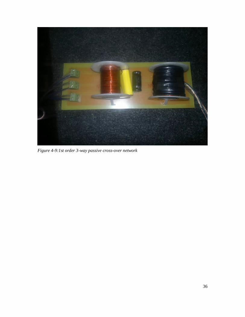
Figure 4-9:1st order 3-way passive cross-over network

37

CHAPTER 5

5 CONCLUSION AND RECOMMENDATIONS

5.1 CONCLUSION

The main objective of the project, which was to come up with an efficient power selection method for passive crossover network, was achieved. Through this method I was able to determine speaker wattages for the crossover network implemented. The audio output of the speakers was of high quality since each speaker drive operated on its specified frequency band hence producing the best quality on the basis of its capability. I was able to design first order and second order crossover network and from the analysis I was able to observe the difference between the two networks. I was able to coil my inductors manually using the formula stated above and also using the equipments in the laboratory. The value of the inductor wound slightly deviated from the desired value which was understood to be experimental error.

After completion of the project I have concluded that this method for power selection is efficient and very accurate as compared to the conventional methods used which involved assumptions and estimation. I have also acquired the necessary skills for implementation of a project like time management. I have also applied theory learned in my course work and also the practical skills acquired in school laboratory in the implementation of the project.

5.2 RECOMMENDATIONS

My recommendations for future work are:

Further encouragement of study to generate more methods for power selections of speaker drives not only for passive crossover networks but also active crossover networks which can also be applied commercially.

Further improvement to reduce challenges incurred in designing of crossover network like coming up with a more accurate formula for winding Inductors.

38

REFERENCES

1. Chris D’ambrose . Frequency Range of Human Hearing ‘The Physic Book’, 2003

2. David b. Weems, Designing, Building and Testing your Own Speaker System with Projects, 3rd edition.

3. Olson, Harry F. Autor, Music, Physics and Engineering, 1967.

4. Bies, David A and Hansen, Colin, Engineering Noise Control, 2003

5. AVS Forum> audio> speakers.

6. www. prestonelectronics.com

7. William, Arthur B & Taylor, Fred J, Electronic Filter Design Handbook, 1995. Mc Graw-Hill. ISBN 0-07-070441

8. Internet- Wikipedia

9. Linkwitz Siegfried, Crossovers, 2009

10. www.tempro.com/asp/pubs-asp, Undestanding and designing passive and active crossovers.

APPENDICES

1. Hz= Hertz

2. dB = Decibel

3. SPL= Sound Pressure Level

4. Pa = Pascal

5. KHz =Kilo Hertz

6. µ = micro

7. m = milli

8. H = Henries

39

9. F = Farads

10. Ω = Ohms

11. Π = 3.14

12. R = Resistance

13. L= Inductance

14. C = Capacitance

15. ZO= Impedance

16. fc = Cross over frequency/ Cut off frequency

17. V= Voltage

18. P = Power

19. f = frequency

20. LPF = Low pass filter

21. HPF = High pass filter

22. BPF = Band pass filter

23. FL= Lower cut off frequency

24. FH = Upper cut off frequency

25. W= Watts

26. rms = root mean square