Semi-Automatic Digital Epigraphy from Images with …gfx.cs.princeton.edu/pubs/Berkiten_2015_SDE/epigraphy_NPAR15_low… · Semi-Automatic Digital Epigraphy from Images ... of rock

Non-Photorealistic Animation and Rendering EXPRESSIVE 2015David Mould and Pierre Bénard (Editors)

Semi-Automatic Digital Epigraphy from Images withNormals

Sema Berkiten1, Xinyi Fan1, and Szymon Rusinkiewicz1

1Princeton University, USA

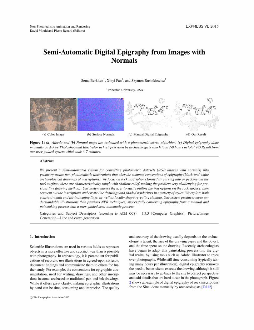
(a) Color Image (b) Surface Normals (c) Manual Digital Epigraphy (d) Our Result

Figure 1: (a) Albedo and (b) Normal maps are estimated with a photometric stereo algorithm. (c) Digital epigraphy donemanually on Adobe Photoshop and Illustrator in high precision by archaeologists which took 7-8 hours in total. (d) Result fromour user-guided system which took 6-7 minutes.

Abstract

We present a semi-automated system for converting photometric datasets (RGB images with normals) intogeometry-aware non-photorealistic illustrations that obey the common conventions of epigraphy (black-and-whitearchaeological drawings of inscriptions). We focus on rock inscriptions formed by carving into or pecking out therock surface: these are characteristically rough with shallow relief, making the problem very challenging for pre-vious line drawing methods. Our system allows the user to easily outline the inscriptions on the rock surface, thensegment out the inscriptions and create line drawings and shaded renderings in a variety of styles. We explore bothconstant-width and tilt-indicating lines, as well as locally shape-revealing shading. Our system produces more un-derstandable illustrations than previous NPR techniques, successfully converting epigraphy from a manual andpainstaking process into a user-guided semi-automatic process.

Categories and Subject Descriptors (according to ACM CCS): I.3.3 [Computer Graphics]: Picture/ImageGeneration—Line and curve generation

1. Introduction

Scientific illustrations are used in various fields to representobjects in a more effective and succinct way than is possiblewith photography. In archaeology, it is paramount for publi-cations of record to use illustrations in agreed-upon styles, todocument findings and communicate them to others for fur-ther study. For example, the conventions for epigraphic doc-umentation, used for writing, drawings, and other inscrip-tions in stone, are based on traditional pen-and-ink drawings.While it offers great clarity, making epigraphic illustrationsby hand can be time-consuming and imprecise. The quality

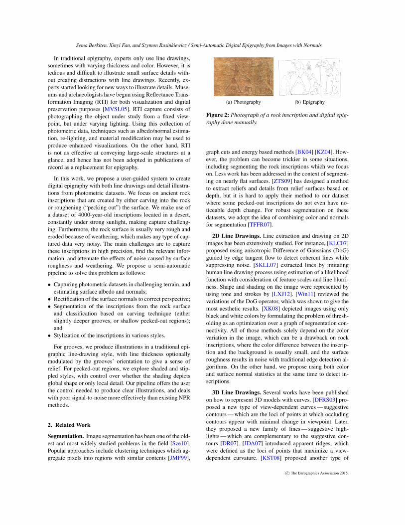
and accuracy of the drawing usually depends on the archae-ologist’s talent, the size of the drawing paper and the object,and the time spent on the drawing. Recently, archaeologistshave begun to adapt this painstaking process into the dig-ital realm, by using tools such as Adobe Illustrator to traceover photographs. While still time-consuming (typically tak-ing many hours per illustration), digital epigraphy removesthe need to be on-site to execute the drawing, although it stillmay be necessary to go back to the site to correct perspectiveand add details that are hard to see in the photograph. Figure2 shows an example of digital epigraphy of rock inscriptionsfrom the Sinai done manually by archaeologists [Tal12].

c© The Eurographics Association 2015.

Sema Berkiten, Xinyi Fan, and Szymon Rusinkiewicz / Semi-Automatic Digital Epigraphy from Images with Normals

In traditional epigraphy, experts only use line drawings,sometimes with varying thickness and color. However, it istedious and difficult to illustrate small surface details with-out creating distractions with line drawings. Recently, ex-perts started looking for new ways to illustrate details. Muse-ums and archaeologists have begun using Reflectance Trans-formation Imaging (RTI) for both visualization and digitalpreservation purposes [MVSL05]. RTI capture consists ofphotographing the object under study from a fixed view-point, but under varying lighting. Using this collection ofphotometric data, techniques such as albedo/normal estima-tion, re-lighting, and material modification may be used toproduce enhanced visualizations. On the other hand, RTIis not as effective at conveying large-scale structures at aglance, and hence has not been adopted in publications ofrecord as a replacement for epigraphy.

In this work, we propose a user-guided system to createdigital epigraphy with both line drawings and detail illustra-tions from photometric datasets. We focus on ancient rockinscriptions that are created by either carving into the rockor roughening (“pecking out”) the surface. We make use ofa dataset of 4000-year-old inscriptions located in a desert,constantly under strong sunlight, making capture challeng-ing. Furthermore, the rock surface is usually very rough anderoded because of weathering, which makes any type of cap-tured data very noisy. The main challenges are to capturethese inscriptions in high precision, find the relevant infor-mation, and attenuate the effects of noise caused by surfaceroughness and weathering. We propose a semi-automaticpipeline to solve this problem as follows:

• Capturing photometric datasets in challenging terrain, andestimating surface albedo and normals;• Rectification of the surface normals to correct perspective;• Segmentation of the inscriptions from the rock surface

and classification based on carving technique (eitherslightly deeper grooves, or shallow pecked-out regions);and• Stylization of the inscriptions in various styles.

For grooves, we produce illustrations in a traditional epi-graphic line-drawing style, with line thickness optionallymodulated by the grooves’ orientation to give a sense ofrelief. For pecked-out regions, we explore shaded and stip-pled styles, with control over whether the shading depictsglobal shape or only local detail. Our pipeline offers the userthe control needed to produce clear illustrations, and dealswith poor signal-to-noise more effectively than existing NPRmethods.

2. Related Work

Segmentation. Image segmentation has been one of the old-est and most widely studied problems in the field [Sze10].Popular approaches include clustering techniques which ag-gregate pixels into regions with similar contents [JMF99],

(a) Photography (b) Epigraphy

Figure 2: Photograph of a rock inscription and digital epig-raphy done manually.

graph cuts and energy based methods [BK04] [KZ04]. How-ever, the problem can become trickier in some situations,including segmenting the rock inscriptions which we focuson. Less work has been addressed in the context of segment-ing on nearly flat surfaces. [ZTS09] has designed a methodto extract reliefs and details from relief surfaces based ondepth, but it is hard to apply their method to our datasetwhere some pecked-out inscriptions do not even have no-ticeable depth change. For robust segmentation on thesedatasets, we adopt the idea of combining color and normalsfor segmentation [TFFR07].

2D Line Drawings. Line extraction and drawing on 2Dimages has been extensively studied. For instance, [KLC07]proposed using anisotropic Difference of Gaussians (DoG)guided by edge tangent flow to detect coherent lines whilesuppressing noise. [SKLL07] extracted lines by imitatinghuman line drawing process using estimation of a likelihoodfunction with consideration of feature scales and line blurri-ness. Shape and shading on the image were represented byusing tone and strokes by [LXJ12]. [Win11] reviewed thevariations of the DoG operator, which was shown to give themost aesthetic results. [XK08] depicted images using onlyblack and white colors by formulating the problem of thresh-olding as an optimization over a graph of segmentation con-nectivity. All of those methods solely depend on the colorvariation in the image, which can be a drawback on rockinscriptions, where the color difference between the inscrip-tion and the background is usually small, and the surfaceroughness results in noise with traditional edge detection al-gorithms. On the other hand, we propose using both colorand surface normal statistics at the same time to detect in-scriptions.

3D Line Drawings. Several works have been publishedon how to represent 3D models with curves. [DFRS03] pro-posed a new type of view-dependent curves — suggestivecontours — which are the loci of points at which occludingcontours appear with minimal change in viewpoint. Later,they proposed a new family of lines — suggestive high-lights — which are complementary to the suggestive con-tours [DR07]. [JDA07] introduced apparent ridges, whichwere defined as the loci of points that maximize a view-dependent curvature. [KST08] proposed another type of



view independent curve: demarcating curves, which are thezeros of the normal curvature in the curvature gradient di-rection. [KST09] defined relief edges as the zero crossingsof the normal curvature in the direction perpendicular to therelief edge. [KST13] extended multi-scale edge detection onimages to 3D surfaces by determining the optimal scale foreach point on the surface. These methods only use the ge-ometry to find the extrema points, which can fail if the in-scriptions are shallow and the surface is rough.

Shape Illustration. There are various non-photorealistictechniques in the literature to depict a shape from 2/2.5/3Dimages. For instance, [KMI∗09] generated a stippling tex-ture on an image from input samples by measuring a tex-ture similarity metric. [TFFR07] investigated various non-photorealistic illustrations on 2.5D images (images with nor-mals). [BMS∗10] used Hermite Radial Basis Function Im-plicits to generate a robust distribution of points on a given3D surface to position the drawing primitives, which arethen rendered to depict shape and tone using silhouetteswith hidden-line attenuation, drawing directions, and stip-pling. [VBGS08] proposed a view-dependent shape descrip-tor called apparent relief, which combines the convexity ofthe 3D object and the normal variations in image-space.Several works focused on using varying line/stroke thick-ness to depict a 3D shape. [SPCP03] extracted and renderedfeature edges by varying the thickness based on perceivedcurvature of the 3D model and [SFWS03] used pen strokesto depict the 3D shape by making them thicker at certaincurvatures, junctions and creases. [HS07] mimicked the hu-man drawing process by following the connectivity of thefeature edges and rendering them using a ribbon metaphor,where the thickness is determined by the twist of the rib-bon. [GVH07] computed the stroke thickness of contoursand suggestive contours from depth, radial curvature, andlight direction.

The previous works have been tailored to work with onlyeither color or geometry information. However, we believethat the archaeological illustrations such as epigraphy repre-sent not only the geometry of the artifact, but also variationsin texture. We can use the photometric data for both geom-etry and texture information (normal maps and albedo ex-tracted from the photometric data, respectively). Examplesof why we need both sources of information are shown inFigure 3. [BSMG05] and [TFFR07] showed how to use pho-tometric data for stylized non-photo realistic renderings. Theformer produces geometry and tone-aware hatching-like ren-derings; while the latter explores how to reformulate someprevious work, such as suggestive contours and ridges andvalley lines, for photometric data. Unfortunately, neither ofthese produces good results for archaeological illustrations.They are either incomplete or noisy, as we will show in Sec-tion 7.

3. Overview

Our main challenge is to produce meaningful (shape-indicating), relevant (including the most representative fea-tures) drawings of archaeological inscriptions. Unfortu-nately, the signal-to-noise ratio is typically low: the inscrip-tions are shallow, while there is considerable noise causedby surface roughness. We briefly review how our datasetsare acquired and rectified (Section 4), then divide the prob-lem into two major components: finding and classifyingthe inscriptions with user-guided segmentation (Section 5),and then rendering them in different geometry-aware non-photorealistic styles (Section 6). We present results on anumber of datasets, and argue that this type of stylizationis difficult to achieve with previous methods (Section 7).

4. Data Acquisition and Preprocessing

We begin with datasets captured at an ancient amethyst min-ing site in an area of Upper Egypt called Wadi el Hudi, whichwas documented in 1952 by [Fak52]. The terrain consistsof several hills covered with granite rocks. The inscriptionsare mostly located on the ridges and their position and sur-roundings make them hard to capture. The ridges are steepand the rocks on the ridges are usually loose, which makesit challenging to set up an acquisition system on the ground.Because of the environmental conditions, the recording mustbe done during the day under strong sunlight. Also, carryingheavy equipment or power sources to the site is impractical,since it takes a short hike to reach some of the inscriptions.However, the resolution of the acquisition system should stillbe high, because the inscriptions are mostly on flat surfaceswith shallow depth. For these reasons, the most practicalsetup is one based on a camera and flash, in preference to 3Dacquisition systems such as structured-light scanners, multi-view stereo, or a laser scanner.

The datasets are captured using aphotometric acquisition setup sim-ilar to the one used by Toler-Franklin et al. [TFFR07], asshown at left. Specifically, a se-ries of digital-SLR images of theobject are captured with a fixedcamera position, and a hand-heldflash is moved around the object toobtain different light directions. A

black cloth is used to shade the object and the camera. Sev-eral mirror and white diffuse spheres, which will be usedto estimate the light directions and intensities in each im-age later, are placed next to the object. Also, one image withno flash is taken at the beginning of each capture session,which will be subtracted from all other images with flashto remove ambient lighting as much as possible. After thephotometric datasets are captured, we use a variant of thephotometric stereo algorithm [Woo80] to estimate surfacenormals and the true albedo from those images: example re-



Figure 3: Left column: Color images of some rock inscrip-tions; Right column: Normal maps. Top row: While the in-scriptions are visible on the color image, some of them arenot recognizable on the normal map. Bottom row: Normalmap reveals more information than the color image for someother cases.

sults are shown in Figure 3. In this paper, we show resultsfrom around 10 representative datasets.

4.1. Rectification

One of the important conventions of documenting rockdrawings is that they need to be recorded from a perpendic-ular view to the surface. However, it is not always possibleto place the camera perpendicularly to the surface becauseof the position and height of the object or the steepness ofthe terrain around it. Another problem is that the inscrip-tions sometimes start from one face of the rock and continueon the other. Recording them from an angle will make themlook skewed, and this is not desirable for documentation. Ar-chaeologists usually warp the image to straighten the partsof the image by either eyeballing to flatten these regions, orif they recorded some 3D points via some terrain mappingsystems such as total station, they manually select the con-trol points on the image corresponding to those 3D pointsand rectify the image. However, it is time-consuming to bothcapture those 3D points and rectify the image based on thosepoints.

In our system, we allow the user to rectify the image with-out any extra data. The user can select a nearly planar regionR, by selecting a few points around the region to create aclosed polygon. Given this selection, we automatically rec-tify the region as follows:

~nmean = normalize(

∑(x,y)∈R

N(x,y))

(1)

~r =~nmean ×< 0,0,1 > (2)

α = acos(~nmean ·< 0,0,1 >) (3)

(a) (b) (c)

Figure 4: (a), (b) Rectified inscription and normal mapwhere the planar region to be rectified is defined by user.(c) User defined rotation axis (marked with red arrow) andflattened inscription.

where N is the normal map, ~r is the rotation axis, and α

is the rotation angle. Once the rotation axis and angle arecomputed, the region is rotated around~r and all the normalvalues are rotated accordingly as shown in Figure 4.a and b.This approach assumes that the region is nearly planar whichis the case for most of the datasets. We also allow the user todraw a rotation axis manually by drawing a line on the imageand use this axis instead to rotate the image around, whichrequires two rotation operations: first we rotate the imageso that the average normal along the user-defined rotationaxis would be equal to the z-direction and then we rotate theimage around this fixed rotation axis to make the region flatas shown in Figure 4.c. The user also can control scaling ofthe preselected region after flattening, as done in Figure 4.

5. Segmentation

We focus on rock inscriptions, which can be classified intotwo types: carved grooves, and “pecked out” areas on therock surface.† Their characteristic roughness and incom-pleteness caused by erosion make the creation of epigraphyvery difficult. Existing NPR techniques are insufficient toproduce nice and understandable illustrations for such rockinscriptions. We approach the problem by first performing arobust segmentation to create masks for the two types of in-scriptions, and then stylize them separately. An implemen-tation pipeline for this segmentation part is described in thefollowing subsection, with details described below.

5.1. Implementation Pipeline

Preprocessing includes downsampling, histogram equaliza-tion, and bilateral filtering to reduce noise and increasecontrast between the foreground inscriptions and the back-ground rock surface. Figures 5.a and 5.b show a color imagebefore and after the preprocessing, respectively.

† Pecking-out is a term used to describe areas where the rock sur-face has been roughened to form a design or figure.



(a) (b)

(c) (d)

(e) (f)

(g) (h)

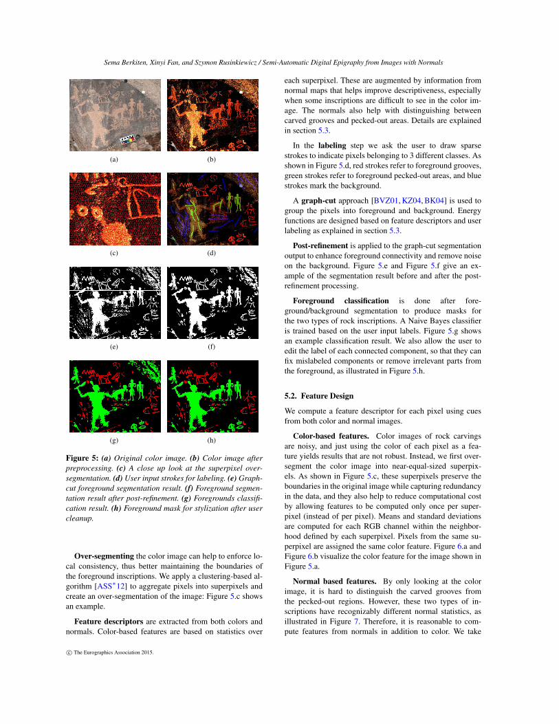
Figure 5: (a) Original color image. (b) Color image afterpreprocessing. (c) A close up look at the superpixel over-segmentation. (d) User input strokes for labeling. (e) Graph-cut foreground segmentation result. (f) Foreground segmen-tation result after post-refinement. (g) Foregrounds classifi-cation result. (h) Foreground mask for stylization after usercleanup.

Over-segmenting the color image can help to enforce lo-cal consistency, thus better maintaining the boundaries ofthe foreground inscriptions. We apply a clustering-based al-gorithm [ASS∗12] to aggregate pixels into superpixels andcreate an over-segmentation of the image: Figure 5.c showsan example.

Feature descriptors are extracted from both colors andnormals. Color-based features are based on statistics over

each superpixel. These are augmented by information fromnormal maps that helps improve descriptiveness, especiallywhen some inscriptions are difficult to see in the color im-age. The normals also help with distinguishing betweencarved grooves and pecked-out areas. Details are explainedin section 5.3.

In the labeling step we ask the user to draw sparsestrokes to indicate pixels belonging to 3 different classes. Asshown in Figure 5.d, red strokes refer to foreground grooves,green strokes refer to foreground pecked-out areas, and bluestrokes mark the background.

A graph-cut approach [BVZ01, KZ04, BK04] is used togroup the pixels into foreground and background. Energyfunctions are designed based on feature descriptors and userlabeling as explained in section 5.3.

Post-refinement is applied to the graph-cut segmentationoutput to enhance foreground connectivity and remove noiseon the background. Figure 5.e and Figure 5.f give an ex-ample of the segmentation result before and after the post-refinement processing.

Foreground classification is done after fore-ground/background segmentation to produce masks forthe two types of rock inscriptions. A Naive Bayes classifieris trained based on the user input labels. Figure 5.g showsan example classification result. We also allow the user toedit the label of each connected component, so that they canfix mislabeled components or remove irrelevant parts fromthe foreground, as illustrated in Figure 5.h.

5.2. Feature Design

We compute a feature descriptor for each pixel using cuesfrom both color and normal images.

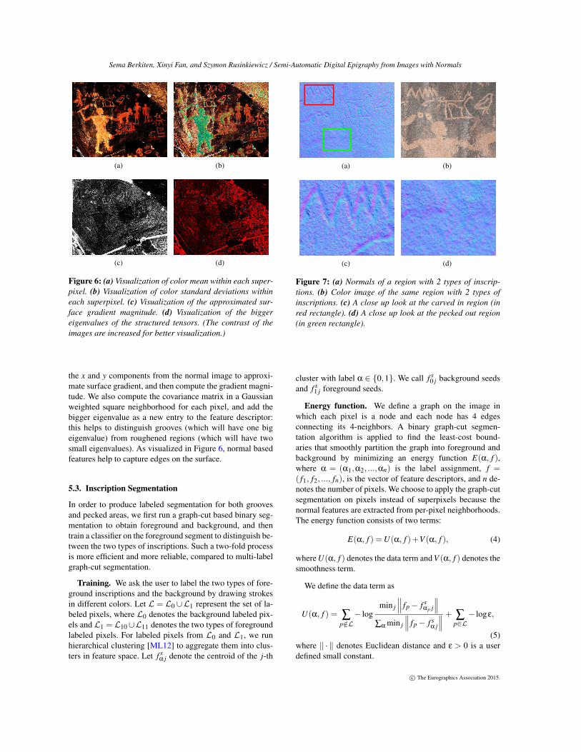
Color-based features. Color images of rock carvingsare noisy, and just using the color of each pixel as a fea-ture yields results that are not robust. Instead, we first over-segment the color image into near-equal-sized superpix-els. As shown in Figure 5.c, these superpixels preserve theboundaries in the original image while capturing redundancyin the data, and they also help to reduce computational costby allowing features to be computed only once per super-pixel (instead of per pixel). Means and standard deviationsare computed for each RGB channel within the neighbor-hood defined by each superpixel. Pixels from the same su-perpixel are assigned the same color feature. Figure 6.a andFigure 6.b visualize the color feature for the image shown inFigure 5.a.

Normal based features. By only looking at the colorimage, it is hard to distinguish the carved grooves fromthe pecked-out regions. However, these two types of in-scriptions have recognizably different normal statistics, asillustrated in Figure 7. Therefore, it is reasonable to com-pute features from normals in addition to color. We take



(a) (b)

(c) (d)

Figure 6: (a) Visualization of color mean within each super-pixel. (b) Visualization of color standard deviations withineach superpixel. (c) Visualization of the approximated sur-face gradient magnitude. (d) Visualization of the biggereigenvalues of the structured tensors. (The contrast of theimages are increased for better visualization.)

the x and y components from the normal image to approxi-mate surface gradient, and then compute the gradient magni-tude. We also compute the covariance matrix in a Gaussianweighted square neighborhood for each pixel, and add thebigger eigenvalue as a new entry to the feature descriptor:this helps to distinguish grooves (which will have one bigeigenvalue) from roughened regions (which will have twosmall eigenvalues). As visualized in Figure 6, normal basedfeatures help to capture edges on the surface.

5.3. Inscription Segmentation

In order to produce labeled segmentation for both groovesand pecked areas, we first run a graph-cut based binary seg-mentation to obtain foreground and background, and thentrain a classifier on the foreground segment to distinguish be-tween the two types of inscriptions. Such a two-fold processis more efficient and more reliable, compared to multi-labelgraph-cut segmentation.

Training. We ask the user to label the two types of fore-ground inscriptions and the background by drawing strokesin different colors. Let L = L0 ∪L1 represent the set of la-beled pixels, where L0 denotes the background labeled pix-els and L1 = L10∪L11 denotes the two types of foregroundlabeled pixels. For labeled pixels from L0 and L1, we runhierarchical clustering [ML12] to aggregate them into clus-ters in feature space. Let f s

α j denote the centroid of the j-th

(a) (b)

(c) (d)

Figure 7: (a) Normals of a region with 2 types of inscrip-tions. (b) Color image of the same region with 2 types ofinscriptions. (c) A close up look at the carved in region (inred rectangle). (d) A close up look at the pecked out region(in green rectangle).

cluster with label α ∈ {0,1}. We call f s0 j background seeds

and f s1 j foreground seeds.

Energy function. We define a graph on the image inwhich each pixel is a node and each node has 4 edgesconnecting its 4-neighbors. A binary graph-cut segmen-tation algorithm is applied to find the least-cost bound-aries that smoothly partition the graph into foreground andbackground by minimizing an energy function E(α, f ),where α = (α1,α2, ...,αn) is the label assignment, f =( f1, f2, ..., fn), is the vector of feature descriptors, and n de-notes the number of pixels. We choose to apply the graph-cutsegmentation on pixels instead of superpixels because thenormal features are extracted from per-pixel neighborhoods.The energy function consists of two terms:

E(α, f ) =U(α, f )+V (α, f ), (4)

where U(α, f ) denotes the data term and V (α, f ) denotes thesmoothness term.

We define the data term as

U(α, f ) = ∑p /∈L− log

min j

∥∥∥ fp− f sαp j

∥∥∥∑α min j

∥∥∥ fp− f sα j

∥∥∥ + ∑p∈L− logε,

(5)where ‖ · ‖ denotes Euclidean distance and ε > 0 is a userdefined small constant.



The smoothness term is defined as

V (α, f ) = γ ∑(p,q)∈N

I(αp 6= αq)e−β( fp− fq)2, (6)

where γ and β are user-defined positive weighting parame-ters.N is the set of neighboring pixel pairs in the grid graph.I(·) is an indicator function that is 1 if αp 6= αq, 0 otherwise.

Cleanup. After the graph-cut segmentation, we performa post-refinement process to enhance foreground connectiv-ity and remove speckles. For each superpixel, we assign thesame label to all pixels within it by taking a majority vote onpixel labels from the graph-cut output. We then remove noisein the background and fill small holes in the foreground byremoving small connected components.

Label classification. Finally, we train a Naive Bayesclassifier [Fuk90] based on feature descriptors of labeledforeground pixels from L1 = L10 ∪ L11, and predict thetype to be either a carved-in or pecked-out inscription. Wethen assign pixels within each connected component withthe same label by conducting a majority vote, and create alabeled segmentation mask for stylization.

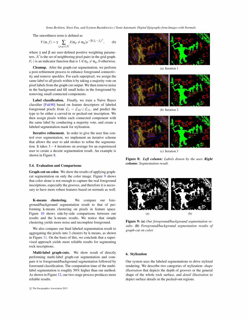
Iterative refinement. In order to give the user fine con-trol over segmentation, we implement an iterative schemethat allows the user to add strokes to refine the segmenta-tion. It takes 3− 4 iterations on average for an experienceduser to create a decent segmentation result. An example isshown in Figure 8.

5.4. Evaluation and Comparisons

Graph-cut on color. We show the results of applying graph-cut segmentation on only the color image. Figure 9 showsthat color alone is not enough to capture the real foregroundinscriptions, especially the grooves, and therefore it is neces-sary to have more robust features based on normals as well.

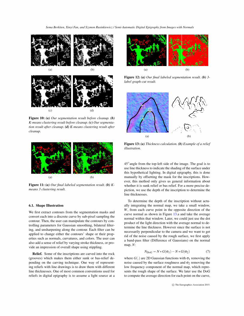
K-means clustering. We compare our fore-ground/background segmentation result to that of per-forming k-means clustering on pixels in feature space.Figure 10 shows side-by-side comparisons between ourresults and the k-means results. We notice that simpleclustering yields more noise and incomplete foreground.

We also compare our final labeled segmentation result toaggregating the pixels into 3 clusters by k-means, as shownin Figure 11. On the basis of this, we conclude that a super-vised approach yields more reliable results for segmentingrock inscriptions.

Multi-label graph-cuts. We show result of directlyperforming multi-label graph-cut segmentation and com-pare it to foreground/background segmentation followed byforeround classification. The computation time of the multi-label segmentation is roughly 50% higher than our method.As shown in Figure 12, our two-stage process produces morereliable results.

(a) Iteration 1

(b) Iteration 2

(c) Iteration 3

Figure 8: Left column: Labels drawn by the user. Rightcolumn: Segmentation result.

(a) (b)

Figure 9: (a) Our foreground/background segmentation re-sults. (b) Foreground/background segmentation results ofgraph-cut on color.

6. Stylization

Our system uses the labeled segmentations to drive stylizedrendering. We describe two categories of stylization: shapeillustration that depicts the depth of grooves or the generalshape of the whole rock surface, and detail illustration todepict surface details in the pecked-out regions.



(a) (b)

(c) (d)

Figure 10: (a) Our segmentation result before cleanup. (b)K-means clustering result before cleanup. (c) Our segmenta-tion result after cleanup. (d) K-means clustering result aftercleanup.

(a) (b)

Figure 11: (a) Our final labeled segmentation result. (b) K-means 3 clustering result.

6.1. Shape Illustration

We first extract contours from the segmentation masks andconvert each into a discrete curve by sub-pixel sampling thecontour. Then, the user can manipulate the contours by con-trolling parameters for Gaussian smoothing, bilateral filter-ing, and unsharpening along the contour. Each filter can beapplied to change either the contours’ shape or their prop-erties such as normals, curvatures, and colors. The user canalso add a sense of relief by varying stroke thickness, or pro-vide an impression of overall shape using stippling.

Relief. Some of the inscriptions are carved into the rock(grooves) which makes them either sunk or bas-relief de-pending on the carving technique. One way of represent-ing reliefs with line drawings is to draw them with differentline thicknesses. One of most common conventions used forreliefs in digital epigraphy is to assume a light source at a

(a) (b)

Figure 12: (a) Our final labeled segmentation result. (b) 3-label graph-cut result.

(a) (b)

Figure 13: (a) Thickness calculation. (b) Example of a reliefillustration.

45◦angle from the top-left side of the image. The goal is touse line thickness to indicate the shading of the surface underthis hypothetical lighting. In digital epigraphy, this is donemanually by offsetting the mask for the inscriptions. How-ever, this method only gives us general information aboutwhether it is sunk relief or bas relief. For a more precise de-piction, we use the depth of the inscription to determine theline thicknesses.

To determine the depth of the inscription without actu-ally integrating the normal map, we take a small window,W , from each curve point in the opposite direction of thecurve normal as shown in Figure 13.a and take the averagenormal within that window. Later, we could just use the dotproduct of the light direction with the average normal to de-termine the line thickness. However since the surface is notnecessarily perpendicular to the camera and we want to getrid of the noise caused by the rough surface, we first applya band-pass filter (Difference of Gaussians) on the normalmap, N:

NDoG = N ∗G(σ1)−N ∗G(σ2) (7)

where G(.) are 2D Gaussian functions with σ1 removing thenoise caused by the surface roughness and σ2 removing thelow frequency component of the normal map, which repre-sents the rough shape of the surface. We later use the DoGto compute the average direction for each point on the curve,



(a) (b)

Figure 14: (a) Stippling on a sphere. (b) Stippling to depictthe rough shape of a curved boulder.

and the thickness is set proportional to the dot product of theaverage DoG and the imaginary light direction.

t(i) =< 1,−1,0 > ·( 1|Wi| ∑

(x,y)∈Wi

NDoG(x,y))

(8)

where t(i) is the computed line thickness at point i. Later, theuser can further smooth the thickness along the curve to havea smoother transition along the contour as described below:

t(i)smooth =1

gtotal

r

∑j=−r

g( j,r)t(i+ j) (9)

where g( j,r) is a Gaussian function in which the varianceof the function is calculated from the maximum range r. InFigure 13.b, an example is shown where the relief illustrationis applied to the grooves while the pecked out regions arerendered with a constant line thickness.

Stippling. To depict the rough shape of the surface, weuse stippling derived from the normal map. We compute thestippling density in small grids by taking the dot product ofthe z direction with the average normal within the grid, W ,as follows:

d = 1−(< 0,0,1 > ·

( 1|W | ∑

(x,y)∈WN(x,y)

))(10)

A number of stippling points proportional to the density arerandomly rendered within the small grid with a color in-versely proportionally to the density. When the surface istilted away from the camera, the stippling density will beclose to one and the color will be darker, and vice versa, asshown for a sphere in Figure 14.a. This method can be usedover all the image when the rock surface is curved to indicatethe general shape of the surface as shown in Figure 14.b.

6.2. Detail Illustration

To illustrate the surface details, we compute the dot productof the surface normals with either the z-direction or the localaverage normal as follows:

I(x,y) =

{d = N(x,y) ·B(x,y) if d < τ

1 otherwise.(11)

where τ is a user defined threshold, which controls the elim-ination of the flatter features and B(x,y) is either < 0,0,1 >or the low frequency component of the normal map, Ng(x,y),computed by Gaussian filtering the normal map. When thez-vector is used, it will depict the general shape of the sur-face such as curviness; on the other hand, if Ng(x,y) is used,it will reveal the local surface details only. If the surface isflat and perpendicular to the camera, both methods will givesimilar results. In our results, extracted details are applied tothe pecked out regions as a texture.

6.3. User Control

The user can control all the sigma and threshold values, andcan use either the albedo, gray tones, or black and white fordetails. The stippling method described in the previous sec-tion can also be used for detail illustration by using Ng(x,y)instead of the z-direction. Different methods for detail illus-tration are shown in Figure 15.

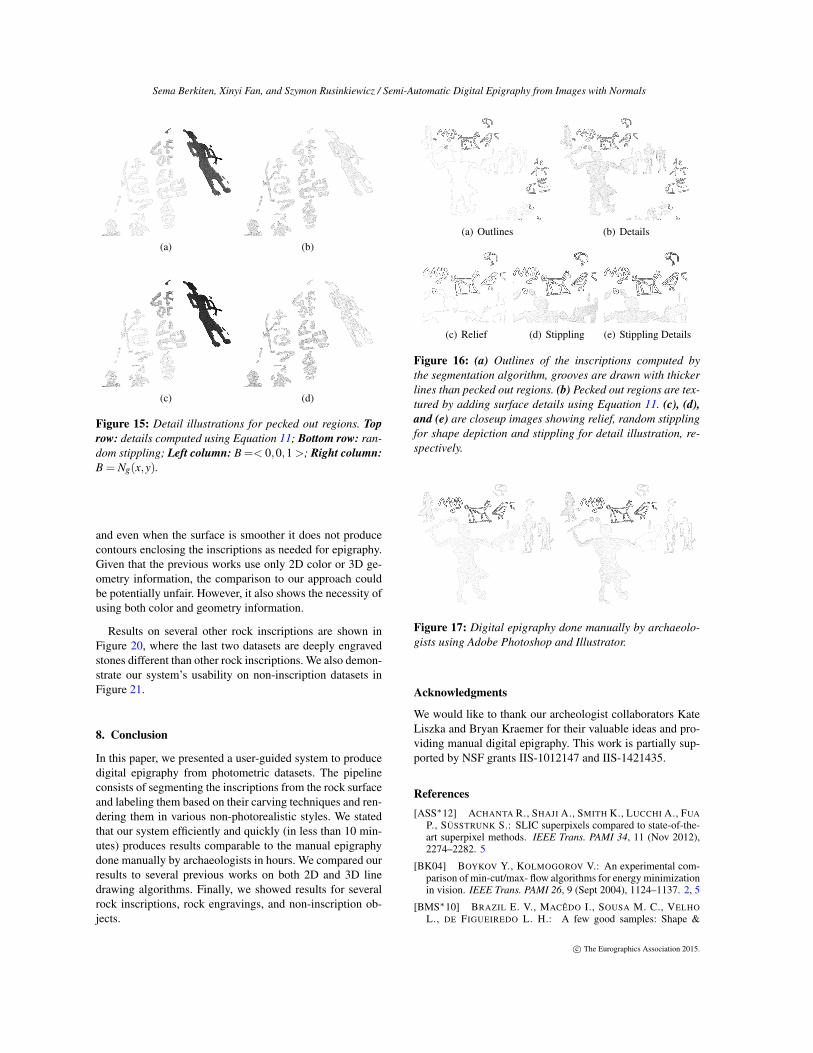
7. Results and Discussion

In this section, we show results on several inscription andnon-inscription datasets, as well as comparisons to some pre-vious work. Figure 16 demonstrates several styles of ourepigraphy pipeline on one dataset. We demonstrate gener-ating outlines of the inscriptions, adding surface details, giv-ing relief effect to the grooves, stippling for shape depiction,and stippling to illustrate the surface details respectively. Forcomparison, Figure 17 shows a digital epigraphy done man-ually by archaeologists in two styles. As they reported, ittook 5-6 hours to trace over the image and another 1-2 hoursto add texture details to the pecked out regions. The mainreason of the manual epigraphy taking such a long time isthe desire for great precision rather than lack of experience.

In Figures 18 and 19, several previous works are com-pared. Results from image-based line drawings are shown inFigure 18, where we compare our result to Coherent LineDrawings (CLD) by [KLC07] and extended Difference ofGaussians (xDoG) by [Win11]. Even though xDoG handlesthe noise caused by surface roughness better than CLD, itfails when the variation in color is small, such as in theright column of the figure. To test 3D line drawing meth-ods, we project the surface normals onto a 3D plane and usethose projected normals to compute 3D contours. As seenin Figure 19, previous works cannot handle the noise well,



(a) (b)

(c) (d)

Figure 15: Detail illustrations for pecked out regions. Toprow: details computed using Equation 11; Bottom row: ran-dom stippling; Left column: B =< 0,0,1 >; Right column:B = Ng(x,y).

and even when the surface is smoother it does not producecontours enclosing the inscriptions as needed for epigraphy.Given that the previous works use only 2D color or 3D ge-ometry information, the comparison to our approach couldbe potentially unfair. However, it also shows the necessity ofusing both color and geometry information.

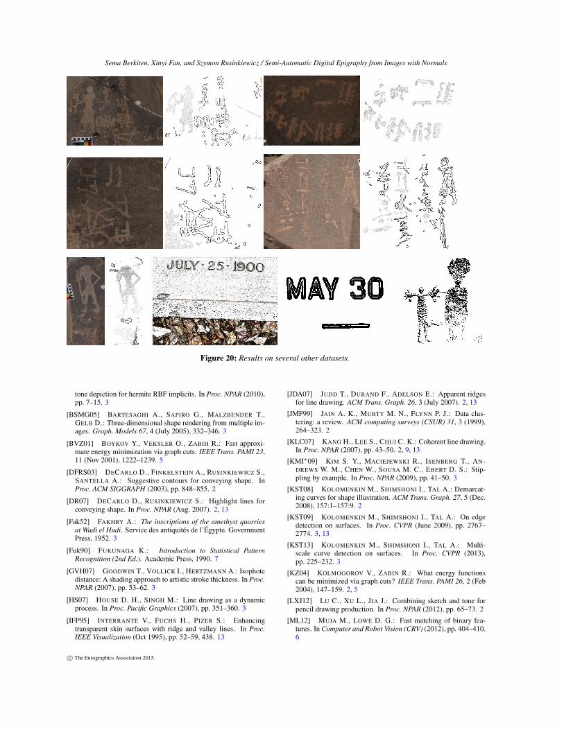
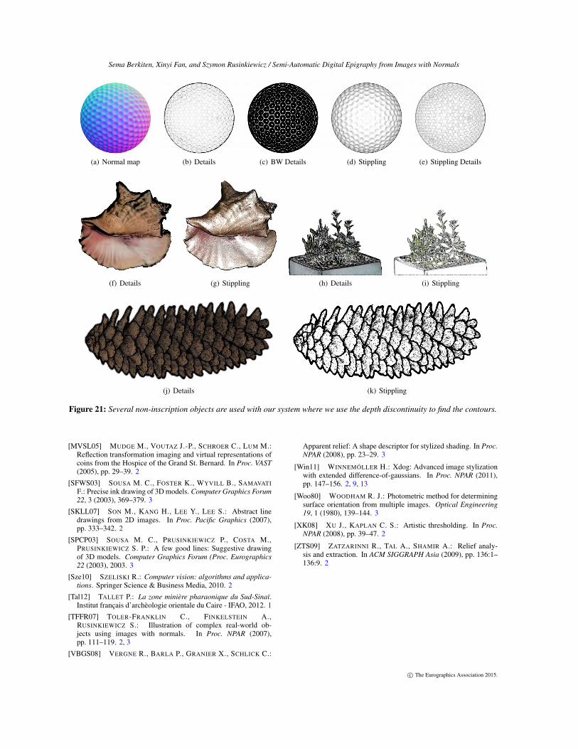
Results on several other rock inscriptions are shown inFigure 20, where the last two datasets are deeply engravedstones different than other rock inscriptions. We also demon-strate our system’s usability on non-inscription datasets inFigure 21.

8. Conclusion

In this paper, we presented a user-guided system to producedigital epigraphy from photometric datasets. The pipelineconsists of segmenting the inscriptions from the rock surfaceand labeling them based on their carving techniques and ren-dering them in various non-photorealistic styles. We statedthat our system efficiently and quickly (in less than 10 min-utes) produces results comparable to the manual epigraphydone manually by archaeologists in hours. We compared ourresults to several previous works on both 2D and 3D linedrawing algorithms. Finally, we showed results for severalrock inscriptions, rock engravings, and non-inscription ob-jects.

(a) Outlines (b) Details

(c) Relief (d) Stippling (e) Stippling Details

Figure 16: (a) Outlines of the inscriptions computed bythe segmentation algorithm, grooves are drawn with thickerlines than pecked out regions. (b) Pecked out regions are tex-tured by adding surface details using Equation 11. (c), (d),and (e) are closeup images showing relief, random stipplingfor shape depiction and stippling for detail illustration, re-spectively.

Figure 17: Digital epigraphy done manually by archaeolo-gists using Adobe Photoshop and Illustrator.

Acknowledgments

We would like to thank our archeologist collaborators KateLiszka and Bryan Kraemer for their valuable ideas and pro-viding manual digital epigraphy. This work is partially sup-ported by NSF grants IIS-1012147 and IIS-1421435.

References[ASS∗12] ACHANTA R., SHAJI A., SMITH K., LUCCHI A., FUA

P., SÜSSTRUNK S.: SLIC superpixels compared to state-of-the-art superpixel methods. IEEE Trans. PAMI 34, 11 (Nov 2012),2274–2282. 5

[BK04] BOYKOV Y., KOLMOGOROV V.: An experimental com-parison of min-cut/max- flow algorithms for energy minimizationin vision. IEEE Trans. PAMI 26, 9 (Sept 2004), 1124–1137. 2, 5

[BMS∗10] BRAZIL E. V., MACÊDO I., SOUSA M. C., VELHOL., DE FIGUEIREDO L. H.: A few good samples: Shape &



Figure 20: Results on several other datasets.

tone depiction for hermite RBF implicits. In Proc. NPAR (2010),pp. 7–15. 3

[BSMG05] BARTESAGHI A., SAPIRO G., MALZBENDER T.,GELB D.: Three-dimensional shape rendering from multiple im-ages. Graph. Models 67, 4 (July 2005), 332–346. 3

[BVZ01] BOYKOV Y., VEKSLER O., ZABIH R.: Fast approxi-mate energy minimization via graph cuts. IEEE Trans. PAMI 23,11 (Nov 2001), 1222–1239. 5

[DFRS03] DECARLO D., FINKELSTEIN A., RUSINKIEWICZ S.,SANTELLA A.: Suggestive contours for conveying shape. InProc. ACM SIGGRAPH (2003), pp. 848–855. 2

[DR07] DECARLO D., RUSINKIEWICZ S.: Highlight lines forconveying shape. In Proc. NPAR (Aug. 2007). 2, 13

[Fak52] FAKHRY A.: The inscriptions of the amethyst quarriesat Wadi el Hudi. Service des antiquités de l’Égypte. GovernmentPress, 1952. 3

[Fuk90] FUKUNAGA K.: Introduction to Statistical PatternRecognition (2nd Ed.). Academic Press, 1990. 7

[GVH07] GOODWIN T., VOLLICK I., HERTZMANN A.: Isophotedistance: A shading approach to artistic stroke thickness. In Proc.NPAR (2007), pp. 53–62. 3

[HS07] HOUSE D. H., SINGH M.: Line drawing as a dynamicprocess. In Proc. Pacific Graphics (2007), pp. 351–360. 3

[IFP95] INTERRANTE V., FUCHS H., PIZER S.: Enhancingtransparent skin surfaces with ridge and valley lines. In Proc.IEEE Visualization (Oct 1995), pp. 52–59, 438. 13

[JDA07] JUDD T., DURAND F., ADELSON E.: Apparent ridgesfor line drawing. ACM Trans. Graph. 26, 3 (July 2007). 2, 13

[JMF99] JAIN A. K., MURTY M. N., FLYNN P. J.: Data clus-tering: a review. ACM computing surveys (CSUR) 31, 3 (1999),264–323. 2

[KLC07] KANG H., LEE S., CHUI C. K.: Coherent line drawing.In Proc. NPAR (2007), pp. 43–50. 2, 9, 13

[KMI∗09] KIM S. Y., MACIEJEWSKI R., ISENBERG T., AN-DREWS W. M., CHEN W., SOUSA M. C., EBERT D. S.: Stip-pling by example. In Proc. NPAR (2009), pp. 41–50. 3

[KST08] KOLOMENKIN M., SHIMSHONI I., TAL A.: Demarcat-ing curves for shape illustration. ACM Trans. Graph. 27, 5 (Dec.2008), 157:1–157:9. 2

[KST09] KOLOMENKIN M., SHIMSHONI I., TAL A.: On edgedetection on surfaces. In Proc. CVPR (June 2009), pp. 2767–2774. 3, 13

[KST13] KOLOMENKIN M., SHIMSHONI I., TAL A.: Multi-scale curve detection on surfaces. In Proc. CVPR (2013),pp. 225–232. 3

[KZ04] KOLMOGOROV V., ZABIN R.: What energy functionscan be minimized via graph cuts? IEEE Trans. PAMI 26, 2 (Feb2004), 147–159. 2, 5

[LXJ12] LU C., XU L., JIA J.: Combining sketch and tone forpencil drawing production. In Proc. NPAR (2012), pp. 65–73. 2

[ML12] MUJA M., LOWE D. G.: Fast matching of binary fea-tures. In Computer and Robot Vision (CRV) (2012), pp. 404–410.6



(a) Normal map (b) Details (c) BW Details (d) Stippling (e) Stippling Details

(f) Details (g) Stippling (h) Details (i) Stippling

(j) Details (k) Stippling

Figure 21: Several non-inscription objects are used with our system where we use the depth discontinuity to find the contours.

[MVSL05] MUDGE M., VOUTAZ J.-P., SCHROER C., LUM M.:Reflection transformation imaging and virtual representations ofcoins from the Hospice of the Grand St. Bernard. In Proc. VAST(2005), pp. 29–39. 2

[SFWS03] SOUSA M. C., FOSTER K., WYVILL B., SAMAVATIF.: Precise ink drawing of 3D models. Computer Graphics Forum22, 3 (2003), 369–379. 3

[SKLL07] SON M., KANG H., LEE Y., LEE S.: Abstract linedrawings from 2D images. In Proc. Pacific Graphics (2007),pp. 333–342. 2

[SPCP03] SOUSA M. C., PRUSINKIEWICZ P., COSTA M.,PRUSINKIEWICZ S. P.: A few good lines: Suggestive drawingof 3D models. Computer Graphics Forum (Proc. Eurographics22 (2003), 2003. 3

[Sze10] SZELISKI R.: Computer vision: algorithms and applica-tions. Springer Science & Business Media, 2010. 2

[Tal12] TALLET P.: La zone minière pharaonique du Sud-Sinaï.Institut français d’archèologie orientale du Caire - IFAO, 2012. 1

[TFFR07] TOLER-FRANKLIN C., FINKELSTEIN A.,RUSINKIEWICZ S.: Illustration of complex real-world ob-jects using images with normals. In Proc. NPAR (2007),pp. 111–119. 2, 3

[VBGS08] VERGNE R., BARLA P., GRANIER X., SCHLICK C.:

Apparent relief: A shape descriptor for stylized shading. In Proc.NPAR (2008), pp. 23–29. 3

[Win11] WINNEMÖLLER H.: Xdog: Advanced image stylizationwith extended difference-of-gaussians. In Proc. NPAR (2011),pp. 147–156. 2, 9, 13

[Woo80] WOODHAM R. J.: Photometric method for determiningsurface orientation from multiple images. Optical Engineering19, 1 (1980), 139–144. 3

[XK08] XU J., KAPLAN C. S.: Artistic thresholding. In Proc.NPAR (2008), pp. 39–47. 2

[ZTS09] ZATZARINNI R., TAL A., SHAMIR A.: Relief analy-sis and extraction. In ACM SIGGRAPH Asia (2009), pp. 136:1–136:9. 2



(a) CLD on Albedo [KLC07]

(b) CLD on Normals [KLC07]

(c) xDoG on Albedo [Win11]

(d) xDoG on Normals [Win11]

(e) Our Results

Figure 18: Comparisons to previous image-based line draw-ing techniques.

(a) Ridges & Valleys [IFP95]

(b) Suggestive Contours & Highlights [DR07]

(c) Apparent Ridges [JDA07]

(d) Relief Edges [KST09]

(e) Isophotes

Figure 19: Comparisons to previous 3D model-based linedrawing techniques.


Documents

Semi-Automatic Digital Epigraphy from Images with …gfx.cs.princeton.edu/pubs/Berkiten_2015_SDE/epigraphy_NPAR15_low… · Semi-Automatic Digital Epigraphy from Images ... of rock