NLR-TP-2000-366

Semi-automatic domain decompositionSemi-automatic domain decompositionSemi-automatic domain decompositionSemi-automatic domain decompositionbased on potential theorybased on potential theorybased on potential theorybased on potential theory

S.P. Spekreijse and J.C. Kok

NationaalNationaalNationaalNationaal Lucht- en Ruimtevaartlaboratorium Lucht- en Ruimtevaartlaboratorium Lucht- en Ruimtevaartlaboratorium Lucht- en RuimtevaartlaboratoriumNational Aerospace Laboratory NLR

NLR-TP-2000-366

Semi-automatic domain decompositionSemi-automatic domain decompositionSemi-automatic domain decompositionSemi-automatic domain decompositionbased on potential theorybased on potential theorybased on potential theorybased on potential theory

S.P. Spekreijse and J.C. Kok

This investigation has been carried out under a contract awarded by Netherlands Agencyfor Aerospace Programmes, contract number 01105N.The Netherlands Agency for Aerospace Programmes has granted NLR permission topublish this report.

This report is based on a presentation to be held at the 7th International Conference onNumerical Grid Generation in Computational Field Simulations, Whistler, Canada,25-28 September 2000.

The contents of this report may be cited on condition that full credit is given to NLR andthe author(s).

Division: Informatics/Fluid Dynamics

Issued: 10 July 2000

Classification of title: Unclassified

- 2 -NLR-TP-2000-366

Summary

Decomposition of a flow domain into blocks, so-called domain decomposition, is the most chal-

lenging task in the process of multi-block grid generation. In this paper, a method is described to

facilitate the construction of the blocks in exterior flow domains. Layers of blocks are automati-

cally generated by solving the Laplace equation in a region between the configuration surface and a

bounding box surface. A boundary element method based on simple-source distributions is used to

solve the Laplace equation. After solving the Laplace equation, starting with a face decomposition

of the configuration surface, blocks are generated by marching along the electrostatic field lines

until a user specified potential is reached. The process may be repeated to generate a second layer

of blocks. However, for configurations with a strongly non-convex shape, some blocks may need

to be added manually to prevent deterioration of the block shapes in the second-layer. Therefore,

the method is called semi-automatic.

-3-NLR-TP-2000-366

Contents

1 Introduction 4

2 Methodology 6

3 The algorithm 8

4 Conclusions 11

5 References 12

19 Figures

(15 pages in total)

- 4 -NLR-TP-2000-366

1 Introduction

Solving the Reynolds-Averaged Navier-Stokes (RANS) equations on continuous multi-block struc-

tured grids has important advantages compared to unstructured grids. Concerning efficiency, for

the same computer memory, multi-block structured flow solvers may use more grid cells than un-

structured flow solvers because no connectivity maps between the grid cells are needed. Further-

more, efficient vectorization and parallelization (on block level) of the flow solver can be rather

easily obtained. Also multi-grid can be applied in a straightforward manner to speed up the con-

vergence rate.

Concerning accuracy, a structured mesh of hexahedral cells is numerically preferable and especially

suitable within the boundary layer where body-fitted cells of large aspect ratio’s (of the order 105)

are needed.

However, multi-block structured grids are considered to be difficult to construct. Especially for

complicated configurations, the subdivision of a flow domain in non-overlapping blocks is a very

labor-intensive task despite the use of advanced graphical interactive programs.

In this paper, a method is presented to facilitate the domain decomposition process. The method

uses concepts as applied in marching grid generation techniques like for example presented in refer-

ences 2, 3. However, many of the problems encountered in marching (hyperbolic) grid generation,

like for example the control about the grid spacing, are of no concern because only blocks are gen-

erated and algebraic or elliptic grid generation methods are used to compute the grids in the blocks

afterwards (Ref. 5).

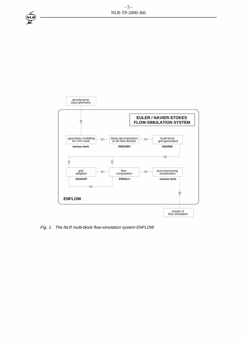
The method has been implemented in the domain decomposer ENDOMO, which is a graphical in-

teractive program for the domain decomposition of arbitrary flow domains in blocks (Ref. 4). EN-

DOMO is part of NLR’s Euler/Navier-Stokes flow simulation system ENFLOW (see Fig. 1, Ref.

6). The system has been employed to simulate flows (both on the basis of the Euler equations and

of the RANS equations) around a large variety of complex aerodynamic configurations, extending

from civil and military aircraft to spacecraft. The grid generator ENGRID is used to compute C0-

continuous structured grids for each block to obtain final multi-block grids. Given aC0-continuous

grid, the flow solver ENSOLV computes the solution of the 3D flow equations based on Euler or

RANS (Refs. 7, 8, 9).

- 5 -NLR-TP-2000-366

FLOW-SIMULATION SYSTEM

results offlow simulation

ENFLOW

EULER / NAVIER-STOKES

block decompositionof 3D flow domain

ENDOMO

grid generation

various tools

aerodynamicinput geometry

geometric modellingfor CFD work

multi-block

gridadaption visualization

post-processing

various toolsENADAP

ENGRID

computationflow

ENSOLV

Fig. 1 The NLR multi-block flow-simulation system ENFLOW

- 6 -NLR-TP-2000-366

2 Methodology

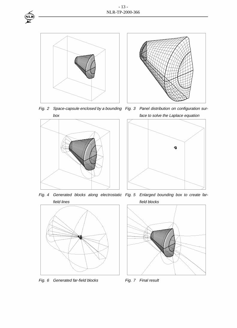
The present method for semi-automatic domain decomposition can probably be best understood

by considering the electrostatic field that would be generated by two perfectly conducting closed

surfaces set at different constant potential values (Ref. 2). One of the surfaces coincides with the

configuration surface and the other surface is a bounding box (a cube), which entirely encloses the

configuration. As an example, figure 2 shows a half-model of a generic space-capsule surrounded

by a bounding box. Assume that the surface of the configuration is subdivided by a non-overlapping

set of faces. Each face is topologically equivalent with a unit square and is bounded by four edges.

The points on the edges of the faces can then be transferred along the electrostatic field lines until

a user-defined potential is reached. In this way, for each face a tube-like block can be generated.

Such a block will then be bounded by the face on the configuration, an opposite face on an equipo-

tential surface, and four faces shaped according to the electrostatic field lines. In this way a layer

of blocks is constructed around the configuration surface. Figure 4 shows the in this way created

blocks around the space-capsule. This approach could be repeated by considering the outer side

of the block layer as the new body shape and by enlarging the bounding box. Figure 5 shows the

enlarged bounding box and figure 6 shows the corresponding far-field block-layer. The method

works well for convex body-shapes like a space-capsule.

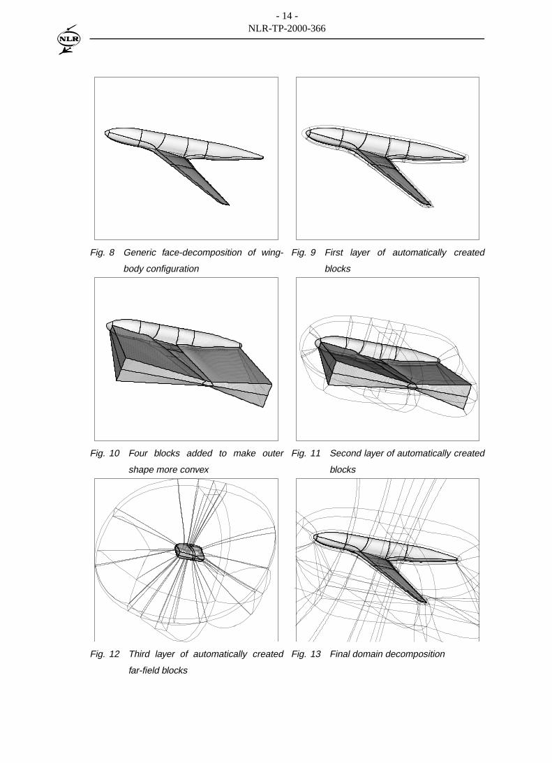
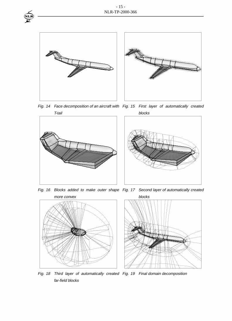
However, this is in general not true for a body with a strongly non-convex shape, like an aircraft, be-

cause then the shape of the blocks may deteriorate, leading to unacceptable grids within the blocks.

The solution to this problem is to add a few blocks so that the outer side of the block layer around

the configuration, together with the added blocks, define a more convex body shape. For this rea-

son, the method is called semi-automatic. The process can then be repeated to construct a second

layer of blocks and also a third far-field layer. All blocks together define a domain decomposition

of the exterior flow domain.

Figure 8 shows a generic face decomposition of a wing-body configuration. Figure 14 shows a

face-decomposition of an aircraft with T-tail. Figure 9 and figure 15 show the corresponding first

layer of blocks around the configurations. The bounding boxes are not shown because again simple

cubes are used. The points on the edges of the faces are transferred along the electrostatic field

lines until a user-specified height is reached (instead of a user-specified potential value which is in

general less suitable for the creation of the first layer of blocks). In this way the first layer of blocks

will have a more or less uniform height. Only points along the edges of the blocks are stored (wire-

frame). The blocks in the first layer will contain the grid boundary layer and are therefore called

Navier-Stokes blocks. The first layer of blocks will contain C-type and O-type blocks. The user-

- 7 -NLR-TP-2000-366

specified block height can not be taken to large because the shape of the blocks may then deteriorate

leading to unacceptable grids within the blocks. This may for example occur near the junction of

the trailing edge and the fuselage.

A few blocks are added such that the outer side of the Navier-Stokes blocks together with the added

blocks define a more convex body shape. Figure 10 shows four added blocks for the wing-body

configuration. Figure 16 shows the added blocks for the T-tail configuration. During the face-

decomposition of the input configuration, the user should have already in mind that these blocks can

be added. This makes the face-decomposition of a complicated configuration surface a non-trivial

task.

Next, the process can be repeated to generate a second-layer of blocks. Of course, the bounding

box must be enlarged. Figure 11 and figure 17 show the second layer for the wing-body and the T-

tail configuration respectively. In both cases, the points along the edges of the faces are transferred

along the electrostatic field lines until a user-specified potential value is reached. Thus the oppo-

site faces will lie on an equipotential surface. The blocks in the second layer will contain no grid

boundary layer and are only used to simulate non-viscous flow features. The blocks are therefore

so-called Euler blocks.

In general, the outer-side of the second layer of Euler blocks defines a convex body shape so that

the process can be easily repeated to generate the far-field Euler blocks. Figure 12 and figure 18

show the far-field blocks.

All blocks together define a non-overlapping domain decomposition of the flow domain. Figure 13

and figure 19 show the final domain decompositions. The total number of blocks for the wing-body

configuration is 98 of which 4 blocks were created manually. The domain decomposition for the

T-tail configuration contains 168 blocks of which 10 blocks were created manually.

The electric field can be computed by solving the Laplace equation in the space between the body

surface and the bounding box. A boundary element method is used to solve the Laplace equation.

Simple source distributions on the body surface and bounding box surface are used to represent

the harmonic function. As an example, figure 3 shows the panel distribution on the surface of the

space-capsule. The panel distribution on the bounding box surface is not shown. Details about the

algorithm are described in the following section.

- 8 -NLR-TP-2000-366

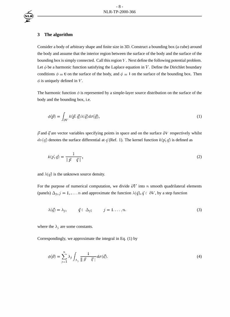
3 The algorithm

Consider a body of arbitrary shape and finite size in 3D. Construct a bounding box (a cube) around

the body and assume that the interior region between the surface of the body and the surface of the

bounding box is simply connected. Call this region V . Next define the following potential problem.

Let � be a harmonic function satisfying the Laplace equation in V . Define the Dirichlet boundary

conditions � � 0 on the surface of the body, and � � 1 on the surface of the bounding box. Then

� is uniquely defined in V .

The harmonic function � is represented by a simple-layer source distribution on the surface of the

body and the bounding box, i.e.

�(~p) =

Z@V

k(~p; ~q)�(~q)d�(~q); (1)

~p and ~q are vector variables specifying points in space and on the surface @V respectively whilst

d�(~q) denotes the surface differential at ~q (Ref. 1). The kernel function k(~p; ~q) is defined as

k(~p; ~q) =1

k ~p� ~q k; (2)

and �(~q) is the unknown source density.

For the purpose of numerical computation, we divide @V into n smooth quadrilateral elements

(panels) �j ; j = 1; : : : ; n and approximate the function �(~q); ~q 2 @V , by a step function

�(~q) = �j; ~q 2 �j; j = 1; : : : ; n; (3)

where the �j are some constants.

Correspondingly, we approximate the integral in Eq. (1) by

�(~p) =nX

j=1

�j

Z�j

1

k ~p� ~q kd�(~q): (4)

- 9 -NLR-TP-2000-366

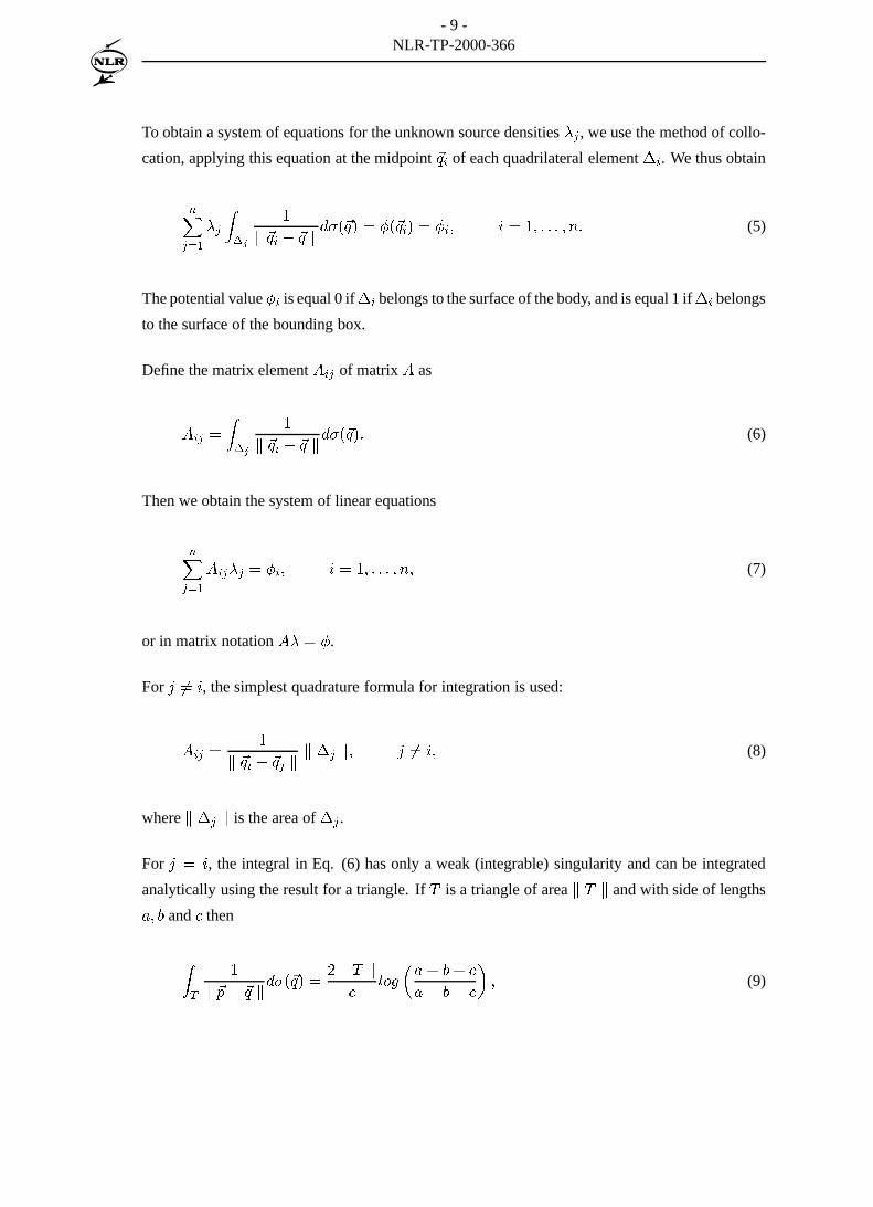
To obtain a system of equations for the unknown source densities �j , we use the method of collo-

cation, applying this equation at the midpoint ~qi of each quadrilateral element �i. We thus obtain

nXj=1

�j

Z�j

1

k ~qi � ~q kd�(~q) = �(~qi) = �i; i = 1; : : : ; n: (5)

The potential value �i is equal 0 if�i belongs to the surface of the body, and is equal 1 if�i belongs

to the surface of the bounding box.

Define the matrix element Aij of matrix A as

Aij =

Z�j

1

k ~qi � ~q kd�(~q): (6)

Then we obtain the system of linear equations

nXj=1

Aij�j = �i; i = 1; : : : ; n; (7)

or in matrix notation A� = �.

For j 6= i, the simplest quadrature formula for integration is used:

Aij =1

k ~qi � ~qj kk �j k; j 6= i; (8)

where k �j k is the area of �j .

For j = i, the integral in Eq. (6) has only a weak (integrable) singularity and can be integrated

analytically using the result for a triangle. If T is a triangle of area k T k and with side of lengths

a; b and c then

ZT

1

k ~p� ~q kd�(~q) =

2 k T k

clog

�a+ b+ c

a+ b� c

�; (9)

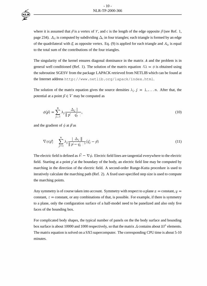
- 10 -NLR-TP-2000-366

where it is assumed that ~p is a vertex of T , and c is the length of the edge opposite ~p (see Ref. 1,

page 234). Aii is computed by subdividing �i in four triangles; each triangle is formed by an edge

of the quadrilateral with ~qi as opposite vertex. Eq. (9) is applied for each triangle and Aii is equal

to the total sum of the contributions of the four triangles.

The singularity of the kernel ensures diagonal dominance in the matrix A and the problem is in

general well conditioned (Ref. 1). The solution of the matrix equation A� = � is obtained using

the subroutine SGESV from the package LAPACK retrieved from NETLIB which can be found at

the Internet address http://www.netlib.org/lapack/index.html.

The solution of the matrix equation gives the source densities �j ; j = 1; : : : ; n. After that, the

potential at a point ~p 2 V may be computed as

�(~p) =nX

j=1

�j

k �j k

k ~p� ~qj k; (10)

and the gradient of � at ~p as

r�(~p) =nX

j=1

�j

k �j k

k ~p� ~qj k3(~qj � ~p) (11)

The electric field is defined as ~E = r�. Electric field lines are tangential everywhere to the electric

field. Starting at a point ~p at the boundary of the body, an electric field line may be computed by

marching in the direction of the electric field. A second-order Runge-Kutta procedure is used to

iteratively calculate the marching path (Ref. 2). A fixed user-specified step size is used to compute

the marching points.

Any symmetry is of course taken into account. Symmetry with respect to a plane x = constant, y =

constant, z = constant, or any combinations of that, is possible. For example, if there is symmetry

to a plane, only the configuration surface of a half-model need to be panelized and also only five

faces of the bounding box.

For complicated body shapes, the typical number of panels on the the body surface and bounding

box surface is about 10000 and 1000 respectively, so that the matrix A contains about 108 elements.

The matrix equation is solved on a SX5 supercomputer. The corresponding CPU time is about 5-10

minutes.

- 11 -NLR-TP-2000-366

4 Conclusions

A method has been developed to compute block layers about arbitrary configurations. For strongly

non-convex configurations, additional blocks must be added to prevent deterioration of the block

shapes. After that, second or third layers of blocks are generated automatically, leading to a satis-

factory domain decomposition of the whole flow domain. The method appears to be an important

tool to reduce the human-time to generate multi-block grids for general 3D configurations. The

user-time to complete the domain-decomposition for a simple geometry, like a space-capsule, takes

a few hours. For a complicated geometry, like an aircraft with T-tail, it takes a few working days. In

general, the time needed for domain decomposition has become comparable with the time needed

for surface modelling (i.e. making a CAD geometry suitable for CFD computations).

- 12 -NLR-TP-2000-366

5 References

1. Jaswon, M.A., Symm, G.T., Integral Equation Methods in Potential Theory and Elastostatics,

Academic Press, 1977.

2. Sikora, J.S., Miranda, L.R., “Boundary Integral Grid Generation Technique”. AIAA 3rd Ap-

plied Aerodynamics Conference, AIAA-85-4088, 1985.

3. Kim, B., Eberhardt, S., “Automatic Multi-Block Grid Generation for High-Lift Configuration

Wings”. In: Surface Modeling, Grid Generation and Related Issues in Computational Fluid

Dynamic (CFD) Solutions, NASA-CP-3291, 1995.

4. Spekreijse, S.P. and Boerstoel, J.W., “Multi-Block Grid Generation”, Von Karman Institute for

Fluid Dynamics (VKI), 27th CFD Course, Lecture Series 1996-02, 1996. (NLR-TP-96338)

5. Spekreijse, S.P., “Elliptic Grid Generation Based on Laplace Equations and Algebraic Trans-

formations”. Journal of Computational Physics 118, 38-61, 1995. (NLR-TP-94102)

6. Boerstoel, J.W., Kassies, A., Kok, J.C., and Spekreijse. S.P., “ENFLOW, a Full-Functionality

System of CFD Codes for Industrial Euler/Navier-Stokes Flow Computations”, presented at

the 2nd Int. Symp. on Aeron. Science and Techn., Jakarta, 1996. (NLR-TP-96286)

7. “A Robust Multi-Block Navier-Stokes Flow Solver for Industrial Applications”, Third ECCO-

MAS CFD Conference, Paris, September 1996. (NLR-TP-96323)

8. Kok, J.C., An Industrially Applicable Solver for Compressible, Turbulent Flows, Ph.D. disser-

tation, Delft University of Technology, 1998.

9. Kok, J.C., Spekreijse, S.P., “Efficient and Accurate Implementation of the k � ! Turbulence

Model in the NLR Multi-Block Navier-Stokes system”, European Congress on Computational

Methods in Applied Sciences and Engineering, ECCOMAS 2000, Barcelona, Spain, Septem-

ber 2000. (NLR-TP-2000-144)

- 13 -NLR-TP-2000-366

Fig. 2 Space-capsule enclosed by a bounding

box

Fig. 3 Panel distribution on configuration sur-

face to solve the Laplace equation

Fig. 4 Generated blocks along electrostatic

field lines

Fig. 5 Enlarged bounding box to create far-

field blocks

Fig. 6 Generated far-field blocks Fig. 7 Final result

- 14 -NLR-TP-2000-366

Fig. 8 Generic face-decomposition of wing-

body configuration

Fig. 9 First layer of automatically created

blocks

Fig. 10 Four blocks added to make outer

shape more convex

Fig. 11 Second layer of automatically created

blocks

Fig. 12 Third layer of automatically created

far-field blocks

Fig. 13 Final domain decomposition

- 15 -NLR-TP-2000-366

Fig. 14 Face decomposition of an aircraft with

T-tail

Fig. 15 First layer of automatically created

blocks

Fig. 16 Blocks added to make outer shape

more convex

Fig. 17 Second layer of automatically created

blocks

Fig. 18 Third layer of automatically created

far-field blocks

Fig. 19 Final domain decomposition