Embed Size (px)
Citation preview
SEMIACTIVE CONTROL OF CIVIL STRUCTURES
FOR NATURAL HAZARD MITIGATION:
ANALYTICAL AND EXPERIMENTAL STUDIES
A Dissertation
Submitted to the Graduate School
of the University of Notre Dame
in Partial Fulfillment of the Requirements
for the Degree of
Doctor of Philosophy
by
Richard E. Christenson, B.S.
B.F. Spencer, Jr., Director
Department of Civil Engineering and Geological Sciences
Notre Dame, Indiana
December 2001
art
ra-
ics of
e mer-
mon-
hods
gs
cou-
are
rfor-
ntrol,
tion
and
stiff-
enti-
e to
SEMIACTIVE CONTROL OF CIVIL STRUCTURES
FOR NATURAL HAZARD MITIGATION:
ANALYTICAL AND EXPERIMENTAL STUDIES
Abstract
by
Richard E. Christenson
The research detailed within this dissertation will investigate innovative sm
structures, including the seismic protection of buildings and the mitigation of wind vib
tions in cable structures. The focus is on understanding the dynamic characterist
these smart structures, identifying viable semiactive control strategies, assessing th
its of the control strategies relative to passive and active control alternatives, and de
strating the structural control concepts. Analytical, numerical and experimental met
are employed in this research.
Coupled building control is shown to be a viable method to protect tall buildin
from seismic excitation. Various coupled building configurations are examined and
pled building design guidelines identified. Constraints on the maximum control force
enforced. A semiactive control strategy applied to a coupled building pair provides pe
mance bounded by passive and active control strategies. Active coupled building co
employing acceleration feedback, is experimentally verified.
The semiactive control of cable structures is examined, studying the vibra
reduction of long cables. The effect of cable sag, axial stiffness, angle of inclination,
damper location on the control performance is examined. Specific levels of sag, axial
ness, angle of inclination, and damper location resulting in poor performance are id
fied. A semiactive control strategy is shown analytically to achieve similar performanc

emi-
ent
ntally
.
hod
uced
vide
ability
Richard E. Christenson
active control, with performance well beyond that achieved with passive control. A s
active control strategy is verified experimentally on a 12.65 meter cable experim
employing a smart shear mode magnetorheological fluid damper. The experime
achieved performance levels are explained by including control-structure interaction
Structural control is shown analytically and experimentally to be a viable met
of protecting civil structures from natural hazards, such as seismic and rain-wind ind
vibration. Semiactive control strategies, when applied to civil structures, can pro
increased performance over passive control without the concerns of energy and st
associated with active control.

ii
To my wife, Kimberly.
Your love and support have been continuous.
For that I am grateful.
. . vii
. . ix
xvi
. . . 1
. . . 3
. . 11
. . 13
16
. . 17
. . 21
. . 32
. 41
. . . 49
1
. . 51
. . 58
. 66
. 70
. 74
. . . 80
CONTENTS
LIST OF TABLES. . . . . . . . . . . . . . . . . . . . . . . . . . . . . . . . . . . . . . . . . . . . . . . . . .
LIST OF FIGURES . . . . . . . . . . . . . . . . . . . . . . . . . . . . . . . . . . . . . . . . . . . . . . . . .
ACKNOWLEDGEMENTS. . . . . . . . . . . . . . . . . . . . . . . . . . . . . . . . . . . . . . . . . . . .
1 INTRODUCTION . . . . . . . . . . . . . . . . . . . . . . . . . . . . . . . . . . . . . . . . . . . . . . . . .
1.1 Structural Control . . . . . . . . . . . . . . . . . . . . . . . . . . . . . . . . . . . . . . . . . . . .
1.2 Semiactive Control Devices . . . . . . . . . . . . . . . . . . . . . . . . . . . . . . . . . . . .
1.3 Overview of Dissertation . . . . . . . . . . . . . . . . . . . . . . . . . . . . . . . . . . . . . .
2 COUPLED BUILDING CONTROL: BACKGROUND . . . . . . . . . . . . . . . . . . . . . .
2.1 Coupled Building Literature Review . . . . . . . . . . . . . . . . . . . . . . . . . . . . .
2.2 Two-Degree-of-Freedom Coupled Building System . . . . . . . . . . . . . . . . .
2.3 2DOF Coupled Building Optimal Passive Control Strategy . . . . . . . . . . .
2.4 Multi-Degree-of-Freedom Coupled Building System . . . . . . . . . . . . . . . . .
2.5 Chapter Summary . . . . . . . . . . . . . . . . . . . . . . . . . . . . . . . . . . . . . . . . . . .
3 COUPLED BUILDING CONTROL: ANALYTICAL STUDIES . . . . . . . . . . . . . . . 5
3.1 Coupled Building Control Strategies . . . . . . . . . . . . . . . . . . . . . . . . . . . . .
3.2 Effects of Building Configuration on RMS Response . . . . . . . . . . . . . . . .
3.3 Efficacy of Semiactive Coupled Building Control . . . . . . . . . . . . . . . . . . . .
3.4 Constraint on Maximum Allowable Control Force . . . . . . . . . . . . . . . . . . .
3.5 Low-Rise Coupled Building System Analysis . . . . . . . . . . . . . . . . . . . . . . .
3.6 Chapter Summary . . . . . . . . . . . . . . . . . . . . . . . . . . . . . . . . . . . . . . . . . . .
iii
. . 84
. 88
. 91
. 93
. . 103
05
. 106
. 108
. 116
. . 119
20
. 120
. . 125
. 130
. . 130
. . 135
. 137
142
. 152
. 155
. 158
. . 166
4 COUPLED BUILDING CONTROL: EXPERIMENTAL VERIFICATION . . . . . . 83
4.1 Coupled Building Experimental Setup . . . . . . . . . . . . . . . . . . . . . . . . . . . .
4.2 Experimental Coupled Building Control-Oriented Design Model . . . . . . . .
4.3 Experimental Active Coupled Building Control Strategy . . . . . . . . . . . . . .
4.4 Experimental Active Coupled Building Results . . . . . . . . . . . . . . . . . . . . . .
4.5 Chapter Summary . . . . . . . . . . . . . . . . . . . . . . . . . . . . . . . . . . . . . . . . . . .
5 CABLE DAMPING CONTROL: BACKGROUND . . . . . . . . . . . . . . . . . . . . . . . . 1
5.1 Cable Damping Literature Review . . . . . . . . . . . . . . . . . . . . . . . . . . . . . . .
5.2 In-Plane Motion of Cable with Sag . . . . . . . . . . . . . . . . . . . . . . . . . . . . . .
5.3 Cable Damping Control Strategies . . . . . . . . . . . . . . . . . . . . . . . . . . . . . . .
5.4 Chapter Summary . . . . . . . . . . . . . . . . . . . . . . . . . . . . . . . . . . . . . . . . . . .
6 CABLE DAMPING CONTROL: EFFECTS OF CABLE SAG . . . . . . . . . . . . . . . 1
6.1 Effects of Sag on Damping Ratio . . . . . . . . . . . . . . . . . . . . . . . . . . . . . . . .
6.2 Effects of Sag on RMS Cable Response. . . . . . . . . . . . . . . . . . . . . . . . . .
6.3 Effects of Sag on Damper Location . . . . . . . . . . . . . . . . . . . . . . . . . . . . . .
6.4 Effects of Sag on Cable Modes. . . . . . . . . . . . . . . . . . . . . . . . . . . . . . . . .
6.5 Chapter Summary . . . . . . . . . . . . . . . . . . . . . . . . . . . . . . . . . . . . . . . . . . .
7 CABLE DAMPING CONTROL: EXPERIMENTAL VERIFICATION . . . . . . . . 137
7.1 Cable Damping Experimental Setup. . . . . . . . . . . . . . . . . . . . . . . . . . . . . .
7.2 System Identification of Cable Damping Model . . . . . . . . . . . . . . . . . . . . .
7.3 Passively-Operated Smart Damping Control Strategy . . . . . . . . . . . . . . . .
7.4 Experimental Semiactive Cable Damping Control Strategy . . . . . . . . . . .
7.5 Experimental Semiactive Cable Damping Results . . . . . . . . . . . . . . . . . . .
7.6 Chapter Summary . . . . . . . . . . . . . . . . . . . . . . . . . . . . . . . . . . . . . . . . . . .
iv
168
. 169
. 174
. . 182
. . 184
. 184
. 186
. . 188
. 190
93
. . 197
. 200
8 INVESTIGATING EXPERIMENTAL AND SIMULATION CABLEDAMPING CONTROL PERFORMANCE . . . . . . . . . . . . . . . . . . . . . . . . . . . . . .
8.1 Investigating Cable Bending Stiffness . . . . . . . . . . . . . . . . . . . . . . . . . . . .
8.2 Investigating Semiactive Cable Damper. . . . . . . . . . . . . . . . . . . . . . . . . . .
8.3 Chapter Summary . . . . . . . . . . . . . . . . . . . . . . . . . . . . . . . . . . . . . . . . . . .
9 CONCLUSIONS . . . . . . . . . . . . . . . . . . . . . . . . . . . . . . . . . . . . . . . . . . . . . . . . . .
9.1 Coupled Building Control Conclusions . . . . . . . . . . . . . . . . . . . . . . . . . . .
9.2 Cable Damping Control Conclusions . . . . . . . . . . . . . . . . . . . . . . . . . . . . .
9.3 Future Studies . . . . . . . . . . . . . . . . . . . . . . . . . . . . . . . . . . . . . . . . . . . . . .
APPENDIX A: Root Mean Square Responses of a First Order Linear Systemusing the Solution to the Lyapunov Equation . . . . . . . . . . . . . . . . . . . . . . . . . . . .
APPENDIX B: Modeling Tall Adjacent Buildings using the Galerkin Method . . . . 1
APPENDIX C: Modeling Tall Adjacent Buildings using the Finite ElementMethod . . . . . . . . . . . . . . . . . . . . . . . . . . . . . . . . . . . . . . . . . . . . . . . . . . . . . . . . .
BIBLIOGRAPHY . . . . . . . . . . . . . . . . . . . . . . . . . . . . . . . . . . . . . . . . . . . . . . . . . .
v
vi
LIST OF TABLES
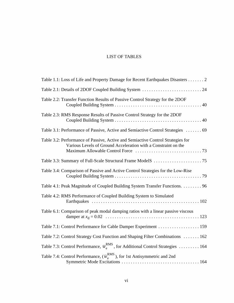
Table 1.1: Loss of Life and Property Damage for Recent Earthquakes Disasters . . . . . . . 2
Table 2.1: Details of 2DOF Coupled Building System . . . . . . . . . . . . . . . . . . . . . . . . . . 24
Table 2.2: Transfer Function Results of Passive Control Strategy for the 2DOFCoupled Building System . . . . . . . . . . . . . . . . . . . . . . . . . . . . . . . . . . . . . . 40
Table 2.3: RMS Response Results of Passive Control Strategy for the 2DOFCoupled Building System . . . . . . . . . . . . . . . . . . . . . . . . . . . . . . . . . . . . . . 40
Table 3.1: Performance of Passive, Active and Semiactive Control Strategies . . . . . . . 69
Table 3.2: Performance of Passive, Active and Semiactive Control Strategies forVarious Levels of Ground Acceleration with a Constraint on theMaximum Allowable Control Force . . . . . . . . . . . . . . . . . . . . . . . . . . . . . 73
Table 3.3: Summary of Full-Scale Structural Frame ModelS . . . . . . . . . . . . . . . . . . . . . 75
Table 3.4: Comparison of Passive and Active Control Strategies for the Low-RiseCoupled Building System . . . . . . . . . . . . . . . . . . . . . . . . . . . . . . . . . . . . . . 79
Table 4.1: Peak Magnitude of Coupled Building System Transfer Functions. . . . . . . . . 96
Table 4.2: RMS Performance of Coupled Building System to SimulatedEarthquakes . . . . . . . . . . . . . . . . . . . . . . . . . . . . . . . . . . . . . . . . . . . . . . . 102
Table 6.1: Comparison of peak modal damping ratios with a linear passive viscousdamper atxd = 0.02 . . . . . . . . . . . . . . . . . . . . . . . . . . . . . . . . . . . . . . . . . 123
Table 7.1: Control Performance for Cable Damper Experiment . . . . . . . . . . . . . . . . . . 159
Table 7.2: Control Strategy Cost Function and Shaping Filter Combinations . . . . . . . 162
Table 7.3: Control Performance, , for Additional Control Strategies . . . . . . . . . 164
Table 7.4: Control Performance, ( ), for 1st Antisymmetric and 2ndSymmetric Mode Excitations . . . . . . . . . . . . . . . . . . . . . . . . . . . . . . . . . . 164
weRMS
weRMS
. . . 2
. . . . 3
. . . . . 5
. . . . 6
. . . . 8
. . 9
. . 20
. . 23
. . 26
. . 27
. . 29
. . 31
. . 35
. . 38
. . 39
. . 39
LIST OF FIGURES
Figure 1.1: Collapse of the original Tacoma Narrows bridge, November 7, 1940. . . .
Figure 1.2: Structural failures during recent strong motion earthquakes. . . . . . . . . .
Figure 1.3: Control strategies and associated supplemental damping devices. . . . .
Figure 1.4: Examples of passive control strategies. . . . . . . . . . . . . . . . . . . . . . . . . . .
Figure 1.5: Examples of active control strategies. . . . . . . . . . . . . . . . . . . . . . . . . . . .
Figure 1.6: Actively controlled Kyobashi Seiwa building in Tokyo, Japan. . . . . . . . . .
Figure 2.1: Examples of full-scale coupled building implementations. . . . . . . . . . . .
Figure 2.2: 2DOF coupled building system undergoing ground excitation and theresulting 2-DOF model. . . . . . . . . . . . . . . . . . . . . . . . . . . . . . . . . . . . . . .
Figure 2.3: Plot of positive complex pole of SDOF system. . . . . . . . . . . . . . . . . . . . .
Figure 2.4: Root locus plot of the 2DOF coupled building system as connectorstiffness and connector damping is varied. . . . . . . . . . . . . . . . . . . . . . . . .
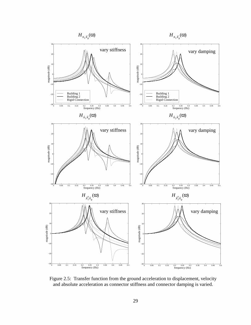
Figure 2.5: Transfer function from the ground acceleration to displacement,velocity and absolute acceleration as connector stiffness andconnector damping is varied. . . . . . . . . . . . . . . . . . . . . . . . . . . . . . . . . . .
Figure 2.6: RMS responses over a range of connector stiffness and connectordamping. . . . . . . . . . . . . . . . . . . . . . . . . . . . . . . . . . . . . . . . . . . . . . . . . . .
Figure 2.7: Optimal transfer functions from ground acceleration to displacementfor the 2DOF undamped coupled building system. . . . . . . . . . . . . . . . . .
Figure 2.8: Optimal poles for the 2DOF coupled building system. . . . . . . . . . . . . . . .
Figure 2.9: Optimal transfer functions of ground acceleration to absoluteaccelerations for the 2DOF coupled building system. . . . . . . . . . . . . . . .
Figure 2.10: Optimal RMS of 2DOF coupled building system. . . . . . . . . . . . . . . . . .
vii
. . 41
. . 45
. . . 47
. . 48
. . 52
. . . 57
. . 60
. . 61
. . 65
. 66
. . . 68
. . . 68
. . 72
. 76
. . 84
. 85
. . 86
. . 89
Figure 2.11: High-rise MDOF coupled building system. . . . . . . . . . . . . . . . . . . . . . .
Figure 2.12: Convergence of undamped natural frequencies for Galerkinand Finite Element methods of the first three modes of each building. . .
Figure 2.13: Power spectral density of ground excitation. . . . . . . . . . . . . . . . . . . . .
Figure 2.14: Estimating RMS ground motions from historical records, wherethe bold section defines the portion of the earthquake used for theRMS calculation. . . . . . . . . . . . . . . . . . . . . . . . . . . . . . . . . . . . . . . . . . . .
Figure 3.1: High-rise MDOF coupled building system for analytical studies. . . . . . .
Figure 3.2: Semiactive damper dissipative forces. . . . . . . . . . . . . . . . . . . . . . . . . . .
Figure 3.3: Frequency analysis of uncoupled 50-, 30- and 20-story buildingresponses, , due to a filtered ground excitation. . . . . . . . . . . . . .
Figure 3.4: Effect of building height and coupling link location on coupled buildingperformance. . . . . . . . . . . . . . . . . . . . . . . . . . . . . . . . . . . . . . . . . . . . . . . .
Figure 3.5: Effect of mass density and stiffness on coupled building performance. . .
Figure 3.6: High-rise MDOF coupled building system for semiactive control. . . . . . .
Figure 3.7: Semiactive coupled building control RMS responses over range ofcontrol forces as compared to passive and active control strategies. . . .
Figure 3.8: RMS response profiles of absolute story acceleration and interstorydrift ratio over the height of both buildings for uncoupled and optimalpassive, active, and semiactive control strategies. . . . . . . . . . . . . . . . . .
Figure 3.9: Semiactive performance with identified maximum allowable controlforce for three levels of excitation as compared to passive and activecontrol strategies. . . . . . . . . . . . . . . . . . . . . . . . . . . . . . . . . . . . . . . . . . . .
Figure 3.10: Beam element, 5- and 3-story building models, and building deflectionfor the low-rise coupled building system. . . . . . . . . . . . . . . . . . . . . . . . . . .
Figure 4.1: Schematic of coupled building experiment. . . . . . . . . . . . . . . . . . . . . . . .
Figure 4.2: Two-story coupled building model for experimental verification. . . . . . . .
Figure 4.3: Control actuator, consisting of a servo-motor with ball-screwmechanism. . . . . . . . . . . . . . . . . . . . . . . . . . . . . . . . . . . . . . . . . . . . . . . . .
Figure 4.4: Comparison of the experimental and curve-fit transfer functions. . . . . . .
Hyewω( )
viii
. . 95
. . . 98
. . . 99
. . 100
. . 101
. . 108
. . 110
. . 118
121
124
126
26
128
128
129
31
. 131
. 132
Figure 4.5: Experimental transfer functions of ground acceleration to absolutestory accelerations. . . . . . . . . . . . . . . . . . . . . . . . . . . . . . . . . . . . . . . . . . .
Figure 4.6: Time history response to El Centro simulated ground acceleration. . . . .
Figure 4.7: Time history response to Hachinohe simulated ground acceleration. . . .
Figure 4.8: Time history response to Northridge simulated ground acceleration. . . .
Figure 4.9: Time history response to Kobe simulated ground acceleration. . . . . . . .
Figure 5.1: In-plane static profilez(x) and dynamic loading f(x,t) of inclined cablewith sag and transverse damper force. . . . . . . . . . . . . . . . . . . . . . . . . . .
Figure 5.2: Typical static sag profiles. . . . . . . . . . . . . . . . . . . . . . . . . . . . . . . . . . . . .
Figure 5.3: Ideal semiactive damper dissipative forces. . . . . . . . . . . . . . . . . . . . . . .
Figure 6.1: Natural frequency and damping ratio in the first two modes for thelinear designs forxd = 0.02. . . . . . . . . . . . . . . . . . . . . . . . . . . . . . . . . . . . .
Figure 6.2: Modal frequency and damping ratios over a range of sag with adamper atxd = 0.02. . . . . . . . . . . . . . . . . . . . . . . . . . . . . . . . . . . . . . . . . . .
Figure 6.3: Frequency and damping ratios of first symmetric mode as a function ofdamper locationxd for several sag levels. . . . . . . . . . . . . . . . . . . . . . . . . .
Figure 6.4: Frequency and damping ratios of first antisymmetric mode as afunction of damper locationxd for several sag levels. . . . . . . . . . . . . . . . . 1
Figure 6.5: RMS displacement for a semiactive, passive viscous, or activedampers atxd = 0.02 as a function of the RMS force. . . . . . . . . . . . . . . . .
Figure 6.6: Minimum RMS displacement for a semiactive, passive viscous, oractive dampers atxd = 0.02. . . . . . . . . . . . . . . . . . . . . . . . . . . . . . . . . . . . .
Figure 6.7: Minimum RMS displacement expanded views near three pairs ofpeaks (xd = 0.02). . . . . . . . . . . . . . . . . . . . . . . . . . . . . . . . . . . . . . . . . . . . .
Figure 6.8: RMS velocity for minimum displacement with a semiactive, passiveviscous, or active damperxd = 0.02. . . . . . . . . . . . . . . . . . . . . . . . . . . . . . . 1
Figure 6.9: RMS displacement with a semiactive, passive viscous, or activedamper at various damper locations. . . . . . . . . . . . . . . . . . . . . . . . . . . . .
Figure 6.10: RMS displacement, relative to the optimal passive linear damper,with an active or semiactive damper at various damper locations. . . . . .
ix
. . 133
e
. 134
. . . 134
. . 138
. . 138
. 139
. . 140
. . . 141
. . 143
. 145
. . 146
. 147
. . 148
. 149
. 150
. . 151
153
. 153
. 155
Figure 6.11: Natural frequencies as a function of the independent parameterλ2
for sag cables. . . . . . . . . . . . . . . . . . . . . . . . . . . . . . . . . . . . . . . . . . . . . .
Figure 6.12: Cable mode shapes at various sag levels. The antisymmetric modes arshown in gray. The natural frequencies (in nondimensional rads/sec) aregiven for the symmetric modes. . . . . . . . . . . . . . . . . . . . . . . . . . . . . . . . .
Figure 6.13: Expanded view of some cable modeshapes. . . . . . . . . . . . . . . . . . . . .
Figure 7.1: Schematic of smart cable damping experiment. . . . . . . . . . . . . . . . . . . .
Figure 7.2: Flat-sag cable experimental setup. . . . . . . . . . . . . . . . . . . . . . . . . . . . . .
Figure 7.3: Brass weights to insure dynamic similitude. . . . . . . . . . . . . . . . . . . . . . . .
Figure 7.4: Smart shear mode magnetorheological fluid damper. . . . . . . . . . . . . . . .
Figure 7.5: Permanent magnet shaker. . . . . . . . . . . . . . . . . . . . . . . . . . . . . . . . . . . .
Figure 7.6: In-plane static profilez(x) and dynamic loading f(x,t) of inclined cablewith sag and transverse damper force. . . . . . . . . . . . . . . . . . . . . . . . . . .
Figure 7.7: Transfer functions comparing flat-sag cable model (black) toexperimental data (grey). . . . . . . . . . . . . . . . . . . . . . . . . . . . . . . . . . . . . .
Figure 7.8: Phenomenological model of shear mode magnetorheological damper. .
Figure 7.9: Comparison of shear mode MR damper analytical model (black) andexperimental data (grey). . . . . . . . . . . . . . . . . . . . . . . . . . . . . . . . . . . . . .
Figure 7.10: Schematic of control signal to permanent magnet shaker. . . . . . . . . . .
Figure 7.11: Comparison of frequency content of actual (experimental) shakerforce to target (analytical). . . . . . . . . . . . . . . . . . . . . . . . . . . . . . . . . . . . .
Figure 7.12: Comparison of frequency content of analytical (solid) and experimental(grey) shaker force. . . . . . . . . . . . . . . . . . . . . . . . . . . . . . . . . . . . . . . . . . .
Figure 7.13: Schematic of process to calculate experimental performancemeasure. . . . . . . . . . . . . . . . . . . . . . . . . . . . . . . . . . . . . . . . . . . . . . . . . .
Figure 7.14: Passively-operated smart damper cable response versus dampervoltage for various levels of excitation. . . . . . . . . . . . . . . . . . . . . . . . . . . .
Figure 7.15: Optimal passively-operated smart damper voltage versus excitationlevel. . . . . . . . . . . . . . . . . . . . . . . . . . . . . . . . . . . . . . . . . . . . . . . . . . . . . .
Figure 7.16: Passively-operated smart damper cable response versus dampervoltage for various modes excited. . . . . . . . . . . . . . . . . . . . . . . . . . . . . . .
x
157
. 158
. 160
161
. 163
. 165
. 170
. 173
. 174
. 175
. . 176
. 176
. . . 179
al. . 179
. 180
. 181
. 182
. . 197
Figure 7.17: Control design filter to weight the spectral content of the shakerexcitation in the H2/LQG control design. . . . . . . . . . . . . . . . . . . . . . . . . . .
Figure 7.18: Actual (grey) damper displacement and zero-mean (black) damperdisplacement used by control strategy. . . . . . . . . . . . . . . . . . . . . . . . . . . .
Figure 7.19: Controller performance at evaluation point and over length of cable. . .
Figure 7.20: Additional control design filters to weight the spectral content ofthe shaker excitation in the H2/LQG control design. . . . . . . . . . . . . . . . . .
Figure 7.21: Controller performance at evaluation point for additional controllers. . .
Figure 7.22: Controller performance at evaluation point for additional cableexcitation. . . . . . . . . . . . . . . . . . . . . . . . . . . . . . . . . . . . . . . . . . . . . . . . . .
Figure 8.1: Profile of cable at different instances in time for smart cable dampingcontrol strategy. . . . . . . . . . . . . . . . . . . . . . . . . . . . . . . . . . . . . . . . . . . . .
Figure 8.2: Effect of bending stiffness () on optimal damping coefficient of passivecable damper for various damper locations. . . . . . . . . . . . . . . . . . . . . . . .
Figure 8.3: Effect of bending stiffness () on achievable modal damping for passiveand active optimal control strategies, and various damper locations. . . .
Figure 8.4: Effect of bending stiffness () on the reduction of RMS response forvarious damper locations. . . . . . . . . . . . . . . . . . . . . . . . . . . . . . . . . . . . . .
Figure 8.5: Force for active, ideal semiactive, and smart dampers. . . . . . . . . . . . . . .
Figure 8.6: Cable damping performance versus damper location including damperdynamics. . . . . . . . . . . . . . . . . . . . . . . . . . . . . . . . . . . . . . . . . . . . . . . . . .
Figure 8.7: Cable damping performance versus arctangent slope parameter . . . . .
Figure 8.8: Comparison of ideal semiactive arctangent damper model to experimentdata. . . . . . . . . . . . . . . . . . . . . . . . . . . . . . . . . . . . . . . . . . . . . . . . . . . . . .
Figure 8.9: Schematic of semiactive arctangent damper model with complianceand corresponding force of each element. . . . . . . . . . . . . . . . . . . . . . . . .
Figure 8.10: Comparison of semiactive arctangent damper model with complianceto experimental data. . . . . . . . . . . . . . . . . . . . . . . . . . . . . . . . . . . . . . . . . .
Figure 8.11: Performance of semiactive arctangent damper model with compliancecompared to previous damper models and experimental results. . . . . . . .
Figure C.1: Degrees-of-freedom for beam element. . . . . . . . . . . . . . . . . . . . . . . . . .
xi

xii
ACKNOWLEDGEMENTS
I would like to thank my advisor, Prof. B.F. Spencer, Jr., for his excellent guidance
and support throughout the course of this research.
I very much appreciate the support and contribution of Prof. E.A. Johnson at the
University of Southern California and Prof. K. Seto at Nihon University, Tokyo, Japan.
I gratefully acknowledge the partial support of this research by the National Sci-
ence Foundation under grant CMS 99-00234 (Dr. S.C. Liu, Program Director), the
National Science Foundation Graduate Research Traineeship Fellowship, and the National
Science Foundation Summer Institute in Japan Program. I also acknowledge support from
industry in the form of equipment and information from the LORD Corporation, Ishikawa-
jima-Harima Heavy Industries Co., LTD., and Quanser Consulting.
Lastly, I want to express my appreciation for the assistance in setting up and con-
ducting my experiments from undergraduates Joseph Winkels, Kimberly Rubeis, Chad
DeBolt, and David Preissler under the National Science Foundation, Research Experi-
ences for Undergraduates (REU) program, and to all my fellow students and researchers
who have helped me in conducting this research.
soci-
s are,
akes,
, both
occu-
oper-
and
. The
vels
the
Two
e the
ay
to the
f the
idge
ode
ised
aug-
CHAPTER 1: INTRODUCTION
Civil structures, such as buildings and bridges, are an integral part of modern
ety. Traditionally, these structures were designed to resist static loads. Civil structure
however, subjected to a variety of dynamic loadings, including winds, waves, earthqu
and traffic. These dynamic loads can cause severe and/or sustained vibratory motion
of which can be detrimental to the structure and its material contents and human
pants. The extent of protection required for these structures may range from reliable
ation and occupancy comfort to human and structural survivability.
An example of a civil structure that required protection for reliable operation
occupancy comfort is the 60-story John Hancock Tower, in Boston, Massachusetts
wind-induced lateral and torsional vibration of the building resulted in acceleration le
too large for occupancy comfort on the upper floors. Additionally, glass panes from
over 10,000 windows of the John Hancock Tower began to fail and fall to the ground.
300 ton tuned mass dampers were installed, in 1977, on the 58th floor to increas
damping ratio of the building and reduce accelerations.
A recent example of a civil structure undergoing vibration is the Trans-Tokyo B
Crossing bridge located in Tokyo, Japan. This steel box-girder bridge was opened
public in December 1997. However, during construction the two longest spans o
bridge, measuring 240 m, experienced significant wind induced vibration of the br
deck due to vortex shedding. The vortex-induced vibration of the first vertical m
resulted in a maximum vibration amplitude of more than 0.5 m. The vibration ra
issues of serviceability, fatigue and yielding failure for the structure. The bridge was
1

deck
is
ma,
f the
of
e died
igure
me of
st 10
.
mented with passive tuned mass dampers to mitigate the vertical motion of the bridge
(Fujino and Yoshida, 2001).
An historic example of a civil structure that did not survive its dynamic loading
the wind induced torsional vibration of the original Tacoma Narrows bridge in Taco
Washington. The vibration of this bridge was so severe that it led to the collapse o
bridge on November 7, 1940, as shown in Figure 1.1.
Civil structures also fail during large seismic events, often resulting in loss
human life and property damage. In recent years, tens of thousands of people hav
and billions of dollars in property damage have been lost as a result of earthquakes. F
1.2 shows the structural damage of civil structures during recent seismic events. So
the most significant earthquakes, in terms of loss of life and loss of property, in the pa
years are listed in Table 1.1.
TABLE 1.1: LOSS OF LIFE AND PROPERTY DAMAGE FOR RECENTEARTHQUAKES DISASTERS
data obtained from the NESDIS National Geophysical Data Center, Significant Earth-quake Database (http://www.ngdc.noaa.gov/seg/hazard/sig_srch.shtml)
Location Date Magnitude Loss of Life Property Damage
Northridge, California 01/17/94 6.8 60 $20 billionKobe, Japan 01/17/95 6.8 5,502 $147 billion
Kocaeli, Turkey 08/17/99 7.8 15,637 $6.5 billionChi-Chi, Taiwan 09/28/99 7.7 2,400 $14 billion
Bhuj, India 01/26/01 8.0 20,005 $4.5 billion
Figure 1.1: Collapse of the original Tacoma Narrows bridge, November 7, 1940
2

haz-
ants,
to
and
con-
inds,
vere
These recent events remind us of the vulnerability of our society to natural
ards. The protection of civil structures, including material content and human occup
is, without doubt, a world-wide priority. The challenge of structural engineers is
develop safer civil structures to better withstand these natural hazards.
1.1 Structural Control
Structural control for civil structures was born out of a need to provide safer
more efficient designs with the reality of limited resources. The purpose of structural
trol is to absorb and to reflect the energy introduced by dynamic loads such as w
waves, earthquakes, and traffic. Today, the protection of civil structures from se
Figure 1.2: Structural failures during recent strong motion earthquakes.
1999 Kocaeli, Turkey Earthquake
1994 Northridge Earthquake 1995 Kobe Earthquake
2001 Bhuj, India Earthquake
3
sider
etic
gy of
tional
lud-
ental
ation
d into
ices is
lass of
e sig-
ctive.
ces in
Fig-
s are
ena,
ond
l be
d sup-
uc-
dynamic loading is typically achieved by allowing the structures to be damaged. Con
the conservation of energy relationship proposed by Uang and Bertero (1988)
(1.1)
where is the total energy input to the structure from the excitation, is the kin
energy of the structure, is the elastic strain energy of the structure, is the ener
the structure dissipated due to inelastic deformation (e.g.,allowing damage to the struc-
ture), and is the energy dissipated by supplemental damping devices. For tradi
structures, the right hand side of Equation (1.1) includes only , , and . By inc
ing the energy term through structural control, the energy dissipated by supplem
damping devices, the kinetic, elastic, and, most importantly, the inelastic deform
energy can be reduced, preserving the primary structure.
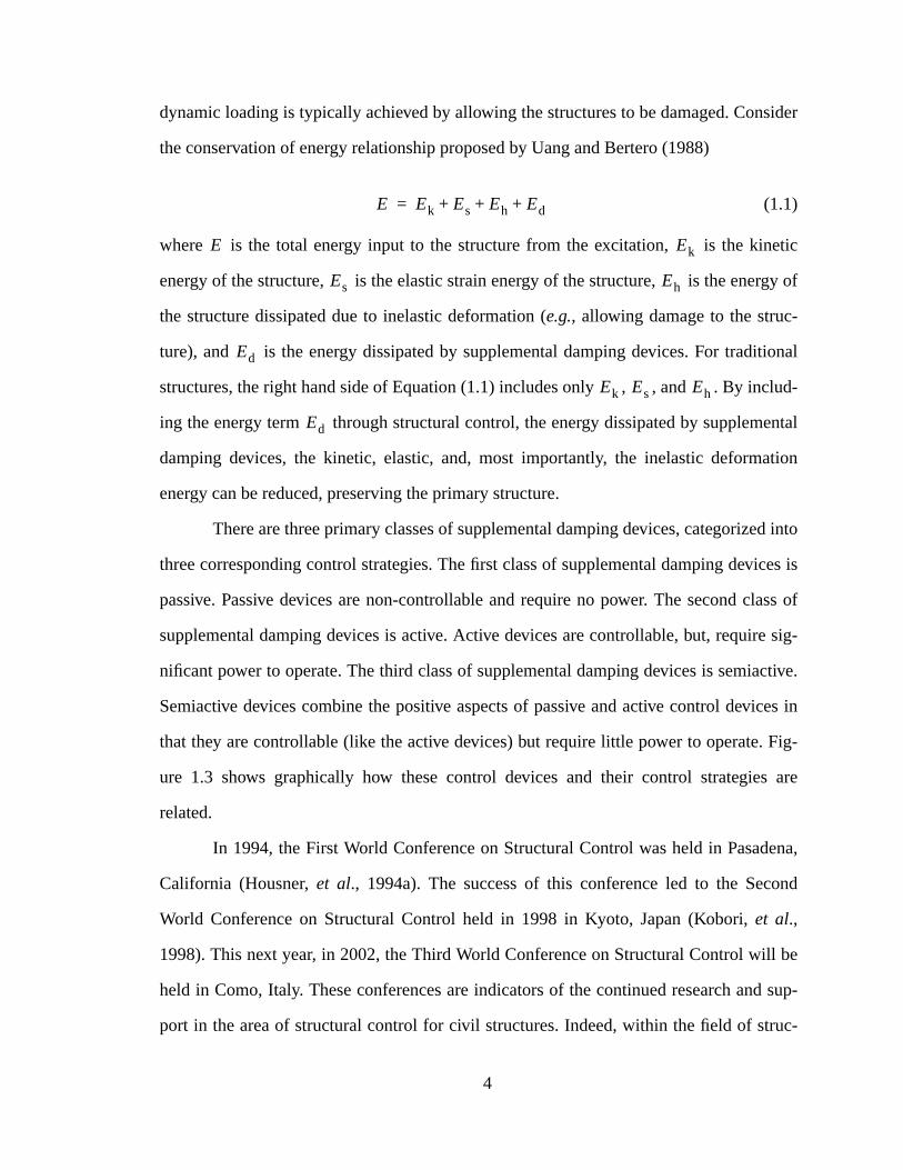
There are three primary classes of supplemental damping devices, categorize
three corresponding control strategies. The first class of supplemental damping dev
passive. Passive devices are non-controllable and require no power. The second c
supplemental damping devices is active. Active devices are controllable, but, requir
nificant power to operate. The third class of supplemental damping devices is semia
Semiactive devices combine the positive aspects of passive and active control devi
that they are controllable (like the active devices) but require little power to operate.
ure 1.3 shows graphically how these control devices and their control strategie
related.
In 1994, the First World Conference on Structural Control was held in Pasad
California (Housner,et al., 1994a). The success of this conference led to the Sec
World Conference on Structural Control held in 1998 in Kyoto, Japan (Kobori,et al.,
1998). This next year, in 2002, the Third World Conference on Structural Control wil
held in Como, Italy. These conferences are indicators of the continued research an
port in the area of structural control for civil structures. Indeed, within the field of str
E Ek Es Eh Ed+ + +=
E Ek
Es Eh
Ed
Ek Es Eh
Ed
4
ental
gy of
rgy
vices
s and
by the
(
cture
bopti-
r opti-
tural control for civil applications, significant research has been conducted, experim
studies performed, and full-scale applications brought to fruition.
Passive Control Strategies
Passive control strategies dissipate and isolate structures from the ener
dynamic loadings (Housner,et al., 1997). In a passive control strategy, a passive ene
dissipation device is attached to the civil structure. Passive energy dissipation de
include metallic, friction, viscoelastic, and viscous fluid dampers, tuned mass damper
tuned liquid dampers (Soong and Dargush, 1997). Passive devices are characterized
dissipative nature of their control forces and the fixed characteristics of the devicese.g.,
damping coefficient). Passive devices are often optimally tuned to protect the stru
from a particular dynamic loading, and thus the performance of these devices is su
mal for other loading scenarios and configurations. For example, a passive dampe
Figure 1.3: Control strategies and associated supplemental damping devices.
PASSIVE DEVICES
non-controllableno power required
ACTIVE DEVICES
controllablesignificant power required
SEMIACTIVE DEVICES
controllablelittle power required
Passive Control Strategies Active Control Strategies
Semiactive Control Strategies
5
educe
base
from
D). A
issi-
levels
own in
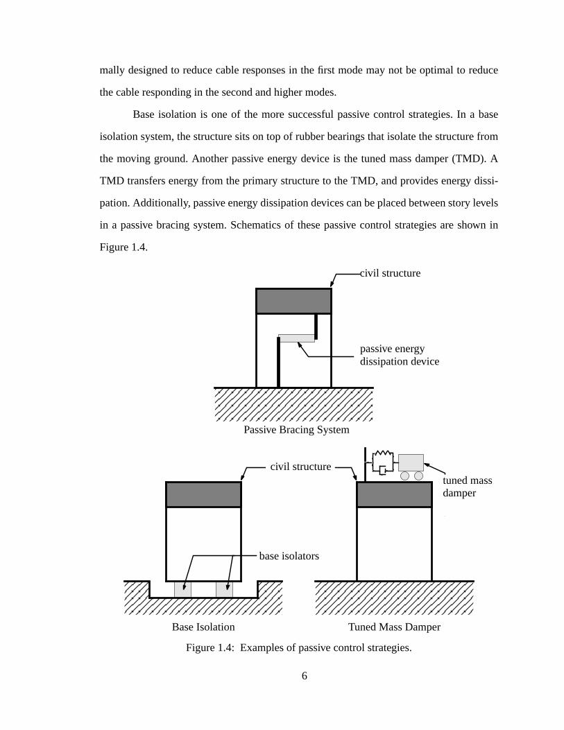
mally designed to reduce cable responses in the first mode may not be optimal to r
the cable responding in the second and higher modes.
Base isolation is one of the more successful passive control strategies. In a
isolation system, the structure sits on top of rubber bearings that isolate the structure
the moving ground. Another passive energy device is the tuned mass damper (TM
TMD transfers energy from the primary structure to the TMD, and provides energy d
pation. Additionally, passive energy dissipation devices can be placed between story
in a passive bracing system. Schematics of these passive control strategies are sh
Figure 1.4.
Figure 1.4: Examples of passive control strategies.
Base Isolation Tuned Mass Damper
civil structure
base isolators
tuned massdamper
civil structure
passive energydissipation device
Passive Bracing System
6

assive
y sim-
times
ular
72)
gies
have
con-
ver
ontrol
s. For
sponse
esti-
As a
ensors
ni-
y of
rategy
duce
e sys-
ctive
hereby
Passive control strategies are popular and have been widely implemented. P
devices are inherently stable, require no external energy to operate and are relativel
ple to design and build. However, the performance of optimal passive control is some
limited, in that they are typically designed protect the structure from one partic
dynamic loading.
Active Control Strategies
At the other extreme of structural control are active control devices. Yao (19
first proposed the active structural control of civil structures. These control strate
deliver force into the structure to counteract the energy of the dynamic loading and
the ability to control different vibration modes and to accommodate different loading
ditions (Housner,et al., 1997). Active devices can provide increased performance o
passive strategies, using global response information to determine appropriate c
forces, in contrast to being limited, as passive devices are, to the local response
example, a passive tuned mass damper must provide control forces based on the re
of the floor where it is located. In contrast, an active control strategy can measure and
mate the response over the entire building to determine appropriate control forces.
result, active control strategies are more complex than passive strategies, requiring s
and evaluator/controller equipment.
Active control devices typically require significant energy to develop the mag
tude of forces required for civil infrastructure applications. The uninterrupted suppl
energy from external sources, especially during natural hazards when the control st
is most expected to operate, is of concern. Active and hybrid control strategies re
unwanted responses by appropriately adding energy to or removing energy from th
tem. However, given a shift in the dynamics of the structure, the performance of the a
strategy may be less than expected and may even result in an unstable condition, w
unbounded energy is specified by the controller.
7
ctive
pencer,
es are
s out a
es of
civil
first
riv-
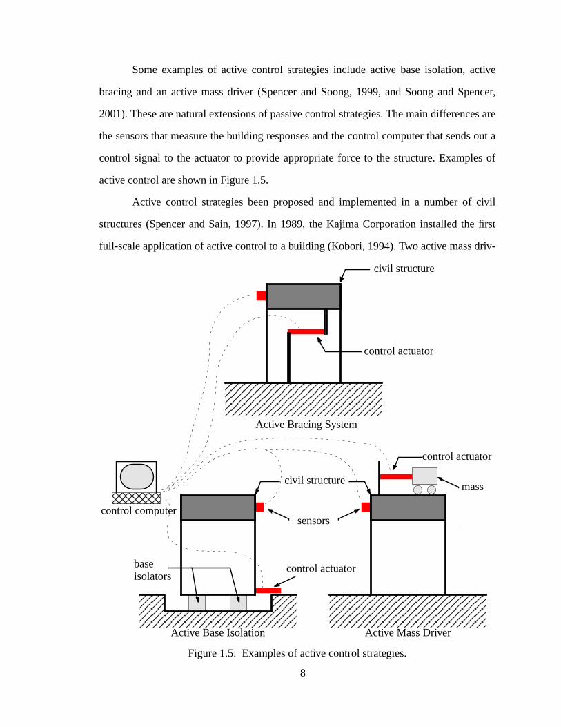
Some examples of active control strategies include active base isolation, a
bracing and an active mass driver (Spencer and Soong, 1999, and Soong and S
2001). These are natural extensions of passive control strategies. The main differenc
the sensors that measure the building responses and the control computer that send
control signal to the actuator to provide appropriate force to the structure. Exampl
active control are shown in Figure 1.5.
Active control strategies been proposed and implemented in a number of
structures (Spencer and Sain, 1997). In 1989, the Kajima Corporation installed the
full-scale application of active control to a building (Kobori, 1994). Two active mass d
Figure 1.5: Examples of active control strategies.
Active Base Isolation Active Mass Driver
civil structure
base
mass
isolators
sensors
control actuator
control actuator
control computer
civil structure
control actuator
Active Bracing System
8
n, to
were
ed on
on-
and
g and
scale
erous
clude,
y and
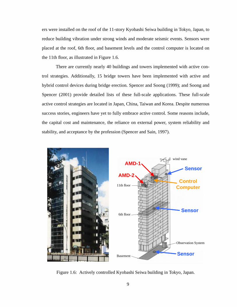
ers were installed on the roof of the 11-story Kyobashi Seiwa building in Tokyo, Japa
reduce building vibration under strong winds and moderate seismic events. Sensors
placed at the roof, 6th floor, and basement levels and the control computer is locat
the 11th floor, as illustrated in Figure 1.6.
There are currently nearly 40 buildings and towers implemented with active c
trol strategies. Additionally, 15 bridge towers have been implemented with active
hybrid control devices during bridge erection. Spencer and Soong (1999); and Soon
Spencer (2001) provide detailed lists of these full-scale applications. These full-
active control strategies are located in Japan, China, Taiwan and Korea. Despite num
success stories, engineers have yet to fully embrace active control. Some reasons in
the capital cost and maintenance, the reliance on external power, system reliabilit
stability, and acceptance by the profession (Spencer and Sain, 1997).
Figure 1.6: Actively controlled Kyobashi Seiwa building in Tokyo, Japan.
AMD-1
AMD-2Control
Computer
Sensor
Sensor
Sensor
AMD-1
AMD-2Control
Computer
Sensor
Sensor
Sensor
Sensor
Sensor
Sensor
wind vane
11th floor
6th floor
Basement
Observation System
9
posi-
egy is
ctly
ssive
sed in
strat-
erate
ing a
low
e and
hieve
mi-
ed in
ally
ance
strat-
mass
ntrol
Semiactive Control Strategies
Semiactive control devices, also called “smart” control devices, assume the
tive aspects of both the passive and active control devices. A semiactive control strat
similar to the active control strategy. Only here, the control actuator does not dire
apply force to the structure, but instead it is used to control the properties of a pa
energy device, a controllable passive damper. Semiactive control strategies can be u
many of the same civil applications as passive and active control. Semiactive control
egies are dissipative in nature, inherently stable, and require a little energy to op
(Spencer and Sain, 1997).
Semiactive control strategies appear to be particularly promising in address
number of the challenges facing active control strategies, in that the devices are
power, fail-safe, and reliable. Semiactive control performance is bounded by passiv
active control. Numerous studies indicate that semiactive control can potentially ac
the majority of the performance of fully active systems. A detailed description of se
active control devices is presented in Section 1.2.
Hybrid Control Strategies
The three primary classes of supplemental damping devices can be combin
various combinations, resulting in hybrid control strategies. Hybrid strategies typic
require less, though still significant, energy. These strategies provide perform
bounded by passive and active control strategies. The most common hybrid control
egy employs the hybrid mass damper (HMD). The HMD combines a passive tuned
damper augmented with an active control actuator. The HMD is the most common co
device for full-scale civil applications.
10
s can
vari-
, etc.
tics of
es can
lth of
civil
rifice
er.
truc-
con-
d for
n pro-
rry,
1.2 Semiactive Control Devices
Semiactive devices are different from active devices in that semiactive device
only produce dissipative forces. Semiactive devices include variable orifice dampers,
able friction dampers, controllable tuned liquid dampers, controllable fluid dampers
These devices can be viewed as controllable passive devices, in that the characteris
the passive devices can be changed in real time. In this manner, semiactive devic
produce the desired dissipative control forces.
This section provides a sampling of the extent of research conducted and wea
literature available on designing and applying various semiactive control devices to
structural applications.
Variable Orifice Damper
The variable orifice damper uses a controllable, electromechanical, variable-o
valve to vary the flow of hydraulic fluid through a conventional hydraulic fluid damp
Variable orifice dampers have been applied to full-scale building (Kobori,et al., 1993;
Kurata,et al., 1999, 2000) and bridge (Sack and Patten, 1994; Patten, 1998, 1999) s
tures.
Variable Friction Damper
Variable friction dampers generate control forces through surface friction and
trolling the slippage of the device. To date, only analytical studies have been conducte
these devices as applied to civil structural control. These devices have, however, bee
posed to reduce interstory drifts of seismically excited buildings (Dowdell and Che
1994; Inaudi, 1997).
11
ith
ncept
hem-
con-
ons
ver,
(MR)
ange
gth
uids
ntly
es of
on,
-
Controllable Tuned Liquid Dampers
Controllable tuned liquid dampers use the motion of a column of fluid, varied w
a controllable orifice, to reduce structural responses. These dampers are similar in co
to tuned mass dampers (TMDs), to absorb the energy of the structure by vibrating t
selves, however, where TMDs are typically designed for one loading condition, the
trollable tuned liquid damper can remain effective for a variety of loading conditi
(Kareem, 1994, Lou,et al., 1994, Yalla and Kareem, 2000).
Controllable Fluid Dampers
Controllable fluid dampers are similar to the variable orifice dampers; howe
they use controllable fluids, such as electrorheological (ER) and magnetorheological
fluids, that do not require a mechanical valve. These ER and MR fluids are able to ch
between free flowing Newtonian fluid and a semi-solid with controllable yield stren
within milliseconds when exposed to electric or magnetic fields, respectively. These fl
date back to the late 1940’s (Winslow, 1947, 1949; and Rabinow, 1948). Only rece
have controllable fluid dampers been proposed for civil applications. Some exampl
literature proposing ER fluids for the application to civil structural control include Burt
et al. (1996), Gavin,et al. (1996a, b), and Makris,et al. (1996). Some examples of litera
ture proposing MR fluids for the application to civil structural control include Dyke,et al.,
(1996a, b, 1998), Spencer,et al., (1997), Jansen and Dyke, (2000), Johnson,et al.,
(2001a, b), Ramallo,et al., (2001), Spencer,et al., (2000), Yi and Dyke, (2000), and
Yoshioka,et al., (2001).
12
the
ced
l for
ined
ains a
ing
ing
d root
identi-
odes
om
oped
Two
ilding
is-
l
ing
ding
cy of
at is
ild-
the
1.3 Overview of Dissertation
This dissertation investigates two innovative semiactive systems. The first is
seismic protection of adjacent buildings. The second is the mitigation of wind indu
vibration of cable structures.
The semiactive control of coupled buildings is investigated, where the potentia
coupling adjacent buildings with semiactive dampers for seismic protection is exam
with respect to active and passive control strategies (Chapters 2-4). Chapter 2 cont
literature review of the history and current status of coupled building control. Follow
this is an examination of a simplified two-degree-of-freedom (2DOF) coupled build
model to understand the effect of coupling on the eigenvalues, transfer functions, an
mean square (RMS) responses of the system. Optimal passive control strategies are
fied for both undamped and damped 2DOF coupled building systems. Since higher m
can contribute to the vibration of tall and flexible buildings, multi-degree-of-freed
(MDOF) building models are also considered. An accurate, low-order, model is devel
for the MDOF coupled building system and a passive control strategy presented.
Chapter 3 details the analytical studies on coupled building control problem.
coupled building control strategies are proposed in this chapter: an active coupled bu
control strategy employingH2/LQG control and absolute acceleration and actuator d
placement feedback; and a semiactive control strategy employing a clipped optimaH2/
LQG control strategy. Next, the effect of building configuration on the coupled build
system is examined. Building configurations such as relative building heights, buil
mass, and building stiffness, as well as the connector location are studied. The effica
semiactive control for the coupled building problem is presented for an example th
similar in configuration to the Triton Square office complex, a set of three high-rise bu
ings in Tokyo, Japan, that were coupled in March 2001. The effect of constraining
maximum allowable control force on system performance is studied.
13
era-
ental
nted
d.
itiga-
rs are
iew of
ping
sive,
erfor-
duced
gne-
. The
ontrol
imen-
e per-
vels of
ntrol
ssible
s, is
ation
solu-
In Chapter 4, active coupled building control employing absolute story accel
tion and actuator displacement feedback is experimentally verified. The experim
setup for the active coupled building control experiment is described, a control orie
model designed, active control strategy identified, and experimental results presente
The second of the complementary research efforts in this dissertation is the m
tion of wind induced vibratory responses of cables (Chapters 5-8). Semiactive dampe
examined to provide transverse control of cables. Chapter 5 contains a literature rev
the history and current status of cable damping control. A model for the cable dam
system with sag is developed.
In Chapter 6, analytical studies on cable damping control are performed. Pas
active and semiactive control strategies are examined. Effects of cable sag on the p
mance of the control strategies are investigated. Regions of cable sag that result in re
levels of performance are identified and explained.
In Chapter 7, semiactive cable damping, employing a smart shear mode ma
torheological fluid damper attached to a 12.6 meter cable, is experimentally verified
experimental setup for the smart cable damping control experiment is described, a c
oriented design model developed, a semiactive control strategy identified, and exper
tal results presented. Various levels and modes of excitation are considered. Also, th
formance of the smart damper operated in a purely passive mode, where constant le
current are supplied to the damper, is examined.
Chapter 8 investigates the experimental and simulation cable damping co
explaining the difference in performance. Two factors are considered to have a po
effect. First, the bending stiffness of the cable, neglected in the simulation studie
examined. Next, the properties of the semiactive damper are examined. This investig
offers an explanation to the difference in cable damping performance and suggests a
tion to experimentally regain this performance.
14

mp-
stud-
Chapter 9 provides conclusions for the coupled building control and cable da
ing control. Additionally, this chapter proposes a number of research areas for future
ies.
15
nbu)
trong
n civil
mate-
ugh
loying
Ultra-
ficult
Cou-
cent
pon
s first
er of
begin-
omen-
e and
this
semi-
CHAPTER 2: COUPLED BUILDING CONTROL: BACKGROUND
Seismic events such as the 1994 Northridge and 1995 Kobe (Hyogo-ken Na
earthquakes are recent reminders of the vulnerability of our cities’ infrastructures to s
motion earthquakes. Strong seismic events can cause severe inelastic behavior i
structures, threatening the safety of occupants and resulting in potential human and
rial losses.
Civil structures are traditionally protected from large seismic events thro
redundancies. In recent years, medium- and high-rise structures have begun emp
control techniques such as active mass drivers (AMDs) to help mitigate responses.
high-rise buildings, such as recent trends are producing, are relatively flexible and dif
to control with AMDs, due to long actuator strokes and large energy requirements.
pling buildings has been shown to be a viable alternative for the protection of adja
flexible structures (Seto, 1994a).
Coupled building control uses dissimilar adjacent structures to impart forces u
one another in such a manner that critical responses are mitigated. This concept wa
introduced by R.E. Klein nearly three decades ago (Klein,et al., 1972). Recently, coupled
building control has received much attention in Japan and the U.S. as a numb
researchers are studying various control strategies, and full-scale applications are
ning to appear.
Over the past three decades, coupled building research has steadily gained m
tum from proposed research concepts to actual implementation. Numerous passiv
active control strategies have been considered for low- to high-rise buildings. In
research, an active control strategy employing acceleration feedback, and, further,
16
-rise
tion
ct of
the
the
d-
pan.
oach,
ck is
tures
sure
is is a
nce-
for
e con-
f the
ssive
ings.
active “smart” dampers, are proposed to connect and control adjacent flexible high
structures.
This chapter contains a literature review of coupled building control, examina
of a simplified two-degree-of-freedom coupled building model to understand the effe
coupling on the dynamic characteristics of the building models, and formulation of
multi-degree-of-freedom coupled building model used for the analytical studies of
research.
2.1 Coupled Building Literature Review
In 1972, Klein, et al. (1972) first proposed the concept of coupling two tall buil
ings in the U.S. In 1976, Kunieda (1976) proposed coupling multiple structures in Ja
In the mid 1980’s, Klein and Healy (1987) suggested a rudimentary semiactive appr
coupling two buildings with cables that could be released and tightened (when sla
available) to provide specified dissipative control forces. They observed that the struc
being coupled with a single link must have different primary natural frequencies to in
controllability. They also proposed that the buildings be connected near the top as th
region where the vibratory modes will have non-zero amplitudes.
In the 1990’s, interest in coupling civil structures was renewed due to adva
ments in structural control and the apparent limits of existing technology (e.g.,base isola-
tors, AMDs,etc.). Graham (1994) coupled single-degree-of-freedom building models
both passive and active control strategies and concluded that, in addition to a passiv
trol strategy, an active LQR control approach can effectively reduce the response o
two coupled buildings. Further studies would continue to show the effectiveness of pa
and active control strategies for the coupled building problem.
Passive control strategies have been studied for both high- and low-rise build
Gurley, et al. (1994), Kamagata,et al. (1996), Fukuda,et al. (1996) and Sakai,et al.
17
vices,
eports
ition-
is
terat-
s.
eto,
l the
igher
a con-
s
hey
ode,
ings
DOF)
sses
or the
-
s able
er of
exible
(1999) have each studied the case of coupling tall flexible structures with passive de
while Luco,et al. (1994, 1998), Xu, et al. (1999a) and Ko,et al. (1999) have studied con-
necting low- to medium-rise structures with passive devices. Each of these papers r
positive results in mitigating the responses due to wind and seismic excitations. Add
ally, Fukuda,et al. noted, as Klein and Healy had implied, that when a coupling link
placed at a node of a vibratory mode, that mode cannot be controlled by the link, rei
ing the importance of the location of the coupling link along the height of the building
Active control strategies have been studied extensively for flexible structures. S
et al. (1994a, 1994b, 1995, 1996, 1998), Haramoto,et al. (1999, 2000), Matsumoto,et al.
(1999), Mitsuta and Seto (1992), Hori and Seto (1999) and Yamada,et al. (1994) have
studied connecting tall flexible structures using active control techniques to contro
long period motion, as well as the higher modes, with encouraging results. The h
modes of flexible structures may be more susceptible to seismic excitations and are
cern for this class of buildings. Seto,et al. have successfully controlled the first two mode
of two and three adjacent flexible building models in simulation and experimentally. T
intentionally placed coupling links at the vibrational nodes of the first neglected m
making it uncontrollable, to prevent spillover of the controller into this higher mode.
In addition to the numerous analytical studies actively coupling adjacent build
for response mitigation, there has been significant experimental work. Mitsuta,et al.
(1992) performed experimental tests on two adjacent single-degree-of-freedom (S
building models and adjacent single- and 2-DOF building models. The building ma
were coupled with an active control actuator, using absolute displacement sensors f
feedback measurement. Yamada,et al. (1994) coupled a pair of 2-story and 3-story build
ing models at the second story with a negative stiffness active control device and wa
to effectively reduce the displacements of these low-rise building models. A numb
experiments have been conducted on coupling two continuous plates, representing fl
high-rise structures (Fukuda,et al. 1996, Hori and Seto, 1999, Kamagata,et al. 1996,
18
ave
ental
of dis-
the
ectro-
s
con-
truc-
ture
uce
on for
control
three
.
and
s, all
ing
story
e 5th
ling
e 12-
pers.
Seto, 1996, 1998, Seto,et al. 1994a, 1994b, 1995). These active control experiments h
used one and two control actuators. The active control strategies for these experim
tests employ displacement measurements for feedback. The direct measurement
placement on large-scale structures is difficult to achieve. Additionally, nearly all of
experimental tests performed to date have produced active control forces using el
magnetic actuators. The exception is Yamada,et al. (1994) who used a spring in serie
with a stepping motor of rack and pinion mechanism to realize their negative stiffness
trol strategy. The idealized actuators have little device dynamics, and thus control-s
ture interaction is not significant in the resulting experiments. Since control-struc
interaction can have a significant effect on the ability of the control actuator to prod
desired forces at the structures resonant frequencies, the inclusion of this phenomen
actuators models more representative of full-scale devices is important (Dyke,et al. 1995).
Numerous papers have been published in Japanese concerning the coupled
of adjacent structures (Ezure,et al. 1993, Ezure,et al. 1994, Ikawa,et al. 1996, Iwanami,
et al. 1986, Iwanami,et al. 1993, Kageyama,et al. 1994, Maeda,et al. 1997, Mitsuta,et
al. 1992, Okawa,et al. 1990, Seto 1998, Seto,et al. 1994c, Sugino,et al. 1997, Toba,et al.
1994, 1995). This research has focused on the passive and active control of two and
adjacent structures, studying roughly the same concepts as the English publications
In addition to these research activities, full-scale tests are being performed
full-scale applications are being realized. Three coupled building control application
located in Japan, are pictured in Figure 2.1. In 1989, the KI (Kajima Intelligent) Build
complex was constructed in Tokyo, Japan. This complex coupled the 5-story and 9-
structures in a low-rise office complex with passive yielding elements connected at th
floor.1 The general contracting firm, Konoike, has implemented four substructure coup
projects in recent years and, in 1998, coupled four of their headquarter buildings, on
story and three 9-story buildings, in Osaka, Japan, with passive visco-elastic dam2
1. Kajima Corporation: Technical pamphlet 91-62E
19

and
Insti-
the
umi
ings,
eight
hree
pro-
Iemura,et al. (1998) has studied passive and active control of two low-rise structures
is preparing full-scale tests to verify the concept at the Disaster Prevention Research
tute (DPRI) in Kyoto, Japan. Here they will connect 3- and 5-story building frames at
3rd floor. The Triton Square office complex, located on the Tokyo waterfront on Har
Island, completed construction in March 2001. The complex is a cluster of three build
195 m, 175 m, and 155 m tall. The 195 m and 175 m tall buildings are coupled at a h
of 160 m. The 175 m and 155 m tall buildings are coupled at a height of 136 m. The t
buildings are coupled with two 35-ton active control actuators for wind and seismic
tection.
2. http://www.konoike.co.jp/
Figure 2.1: Examples of full-scale coupled building implementations.
Kajima Intelligent Building
Triton Square OfficeComplex
ComplexKonoike Headquarter
Buildings
20
lly
larger
is dis-
pre-
tive
ely, to
lems
f-
ee-of-
g to
an sig-
ulti-
ree-
sin-
, and
tud-
Experimental studies to verify active coupled building control have traditiona
employed displacement feedback. The direct measurement of displacements on
scale structures is difficult to achieve, thus acceleration feedback, as considered in th
sertation, is an appealing control strategy for coupled building control.
Active control strategies employing acceleration feedback have been shown in
vious experiments to be effective for other civil structure applications, including an ac
bracing system (Spencer,et al. 1993), an active tendon system (Dyke,et al. 1994a, 1994b)
and active mass driver systems (Dyke,et al. 1996b, Battaini,et al. 2000). In Chapters 3
and 4, acceleration feedback is shown, through simulation and experiment, respectiv
be an effective method of response reduction for the active coupled building prob
(Christenson,et al. 1999b, Hori,et al. 2000).
In Chapter 3, semiactive coupled building control is proposed (Christenson,et al.
1999a, 1999b, 2000a, 2000b, 2000c). Recently Zhu,et al. (2001) have also proposed
semiactive coupled building control. Zhu,et al. consider coupling two single-degree-o
freedom masses with a semiactive connector with positive results. The single-degr
freedom building models in Zhu,et al. do not allow for coupling link position interference
with vibratory nodes to be considered nor for higher mode participation and matchin
be examined. These are important features of the coupled building system, as they c
nificantly effect system performance, and are examined in Chapter 3, using the m
degree-of-freedom (MDOF) building model developed in this chapter.
2.2 Two-Degree-of-Freedom Coupled Building System
The most basic representation of the coupled building problem is the two-deg
of-freedom (2DOF) coupled building system. Here, two buildings, each modeled as a
gle-degree-of-freedom (SDOF) structure, are connected with a passive coupling link
the resulting 2DOF system is examined. This simplified coupled building system is s
21
sys-
ents
nt for
con-
timal
on of
The
ures,
o
.2.
a first
ts a
e 45-
eto,
he dis-
ure.
ied in order to gain valuable insight into the effect of coupling on the dynamics of the
tem.
The passive control strategy involves placing stiffness and damping elem
between the two masses. The selection of an optimal stiffness and damping coefficie
the connector link is critical to the performance of the coupled passive system. When
sidering structures that are both internally damped, a closed-form solution for the op
connector stiffness and connector damping is not readily available. The determinati
the optimal values is accomplished here through an iterative search process.
2DOF Coupled Building Evaluation Model
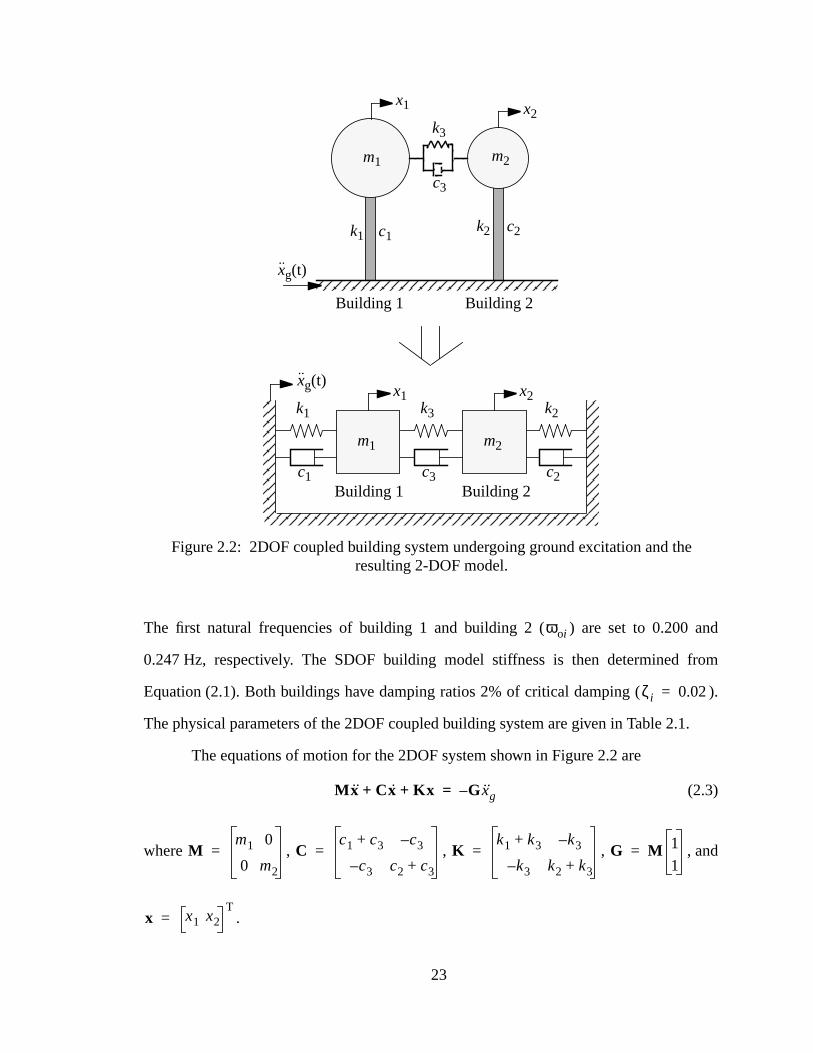
The evaluation model for the 2DOF coupled building system is developed.
coupled building model presented in this section is comprised of two SDOF struct
with mass (m1 andm2), stiffness (k1 andk2) and damping (c1 andc2) associated with each
structure, and a spring and damper (k3 andc3) located in the coupling link between the tw
masses. This system, and the 2DOF model representing it, are depicted in Figure 2
The system parameters are assigned such that the 2DOF system represents
mode analysis of two typical tall buildings. The stiffness and damping for theith building
are related to the natural frequency and damping ratio by
(2.1)
(2.2)
The stiffness and damping of the connector link,k3 andc3, are set by the designer.
Building 1 is intended to represent a 50-story building and building 2 represen
45-story building. The buildings are considered to be connected at the top floor of th
story building. The lumped masses are determined using the eigenvector method (Set
al. 1987), so that the displacement of the lumped masses have physical meaning as t
placement at the coupling link of 50- and 45-story high-rise buildings bending in flex
ωoi ζi
ki ωoi2
mi=
ci 2ζiωoimi=
22
and
rom
).
1.
e
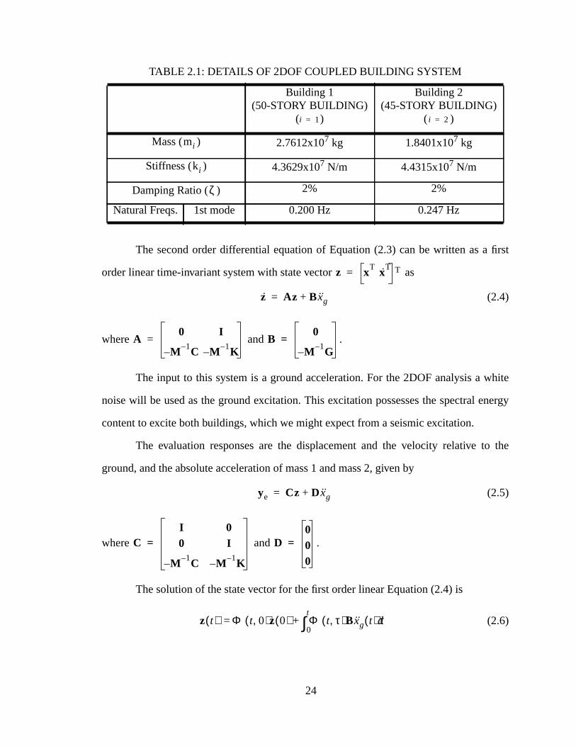
The first natural frequencies of building 1 and building 2 ( ) are set to 0.200
0.247 Hz, respectively. The SDOF building model stiffness is then determined f
Equation (2.1). Both buildings have damping ratios 2% of critical damping (
The physical parameters of the 2DOF coupled building system are given in Table 2.
The equations of motion for the 2DOF system shown in Figure 2.2 are
(2.3)
where , , , , and
.
Figure 2.2: 2DOF coupled building system undergoing ground excitation and thresulting 2-DOF model.
c1k1c2k2
c3
k3
m1 m2
Building 1 Building 2
xg(t)..
c1
k1
c2
k2
c3
k3
m1
x1
m2
x2
Building 1 Building 2
xg(t)..
x1 x2
ωoi
ζi 0.02=
Mx Cx Kx+ + G– xg=
Mm1 0
0 m2
= Cc1 c3+ c– 3
c– 3 c2 c3+= K
k1 k3+ k– 3
k– 3 k2 k3+= G M 1
1=
x x1 x2T
=
23
first
hite
nergy
o the
The second order differential equation of Equation (2.3) can be written as a
order linear time-invariant system with state vector as
(2.4)
where and .
The input to this system is a ground acceleration. For the 2DOF analysis a w
noise will be used as the ground excitation. This excitation possesses the spectral e
content to excite both buildings, which we might expect from a seismic excitation.
The evaluation responses are the displacement and the velocity relative t
ground, and the absolute acceleration of mass 1 and mass 2, given by
(2.5)
where and .
The solution of the state vector for the first order linear Equation (2.4) is
(2.6)
TABLE 2.1: DETAILS OF 2DOF COUPLED BUILDING SYSTEM
Building 1(50-STORY BUILDING)
( )
Building 2(45-STORY BUILDING)
( )
Mass ( ) 2.7612x10⁷ kg 1.8401x10⁷ kg
Stiffness ( ) 4.3629x10⁷ N/m 4.4315x10⁷ N/m
Damping Ratio ( ) 2% 2%
Natural Freqs. 1st mode 0.200 Hz 0.247 Hz
i 1= i 2=
mi
ki
ζ
z xT xT T=
z Az B xg+=
A0 I
M 1– C– M 1– K–= B
0
M 1– G–=
ye Cz Dxg+=
CI 00 I
M–1– C M–
1– K
= D000
=
z t( ) Φ t 0,( )z 0( ) Φ t τ,( )B xg t( ) τd0
t
∫+=
24
is
the
ng
ns of
two
upled
nue to
con-
will
e two
large
ing or
’s)
ome-
se in
sys-
.
lated
ing
ing is
where the state transition (or principal) matrix for time invariant systems
and the initial conditions are given by .
2DOF Coupled Building Root Locus Analysis
A root locus analysis of the 2DOF coupled building system is performed using
eigenvalues of the state spaceA matrix defined in Equation (2.4) and connector dampi
and stiffness are varied. By observing the shift of the coupled system poles as functio
the coupling stiffness and damping, the physical transformation that occurs as the
structures become increasingly coupled can be examined.
As the stiffness and damping of the coupling member increases, the two unco
SDOF structures become a coupled 2DOF system. As the stiffness or damping conti
increase and become significantly large, the two buildings become effectively rigidly
nected and behave as a single SDOF oscillator. The rigidly connected SDOF system
contain a single natural frequency located between the two natural frequencies of th
uncoupled SDOF structures.
The poles of the rigidly connected coupled building system are the same for
connector stiffness or large connector damping. The difference between using a spr
damper in the coupling link is how (the path) and which poles (building 1 or building 2
move from the uncoupled poles to the rigidly connected poles. To observe this phen
non the poles of the 2DOF coupled building system are examined for both an increa
connector stiffness and an increase in connector damping.
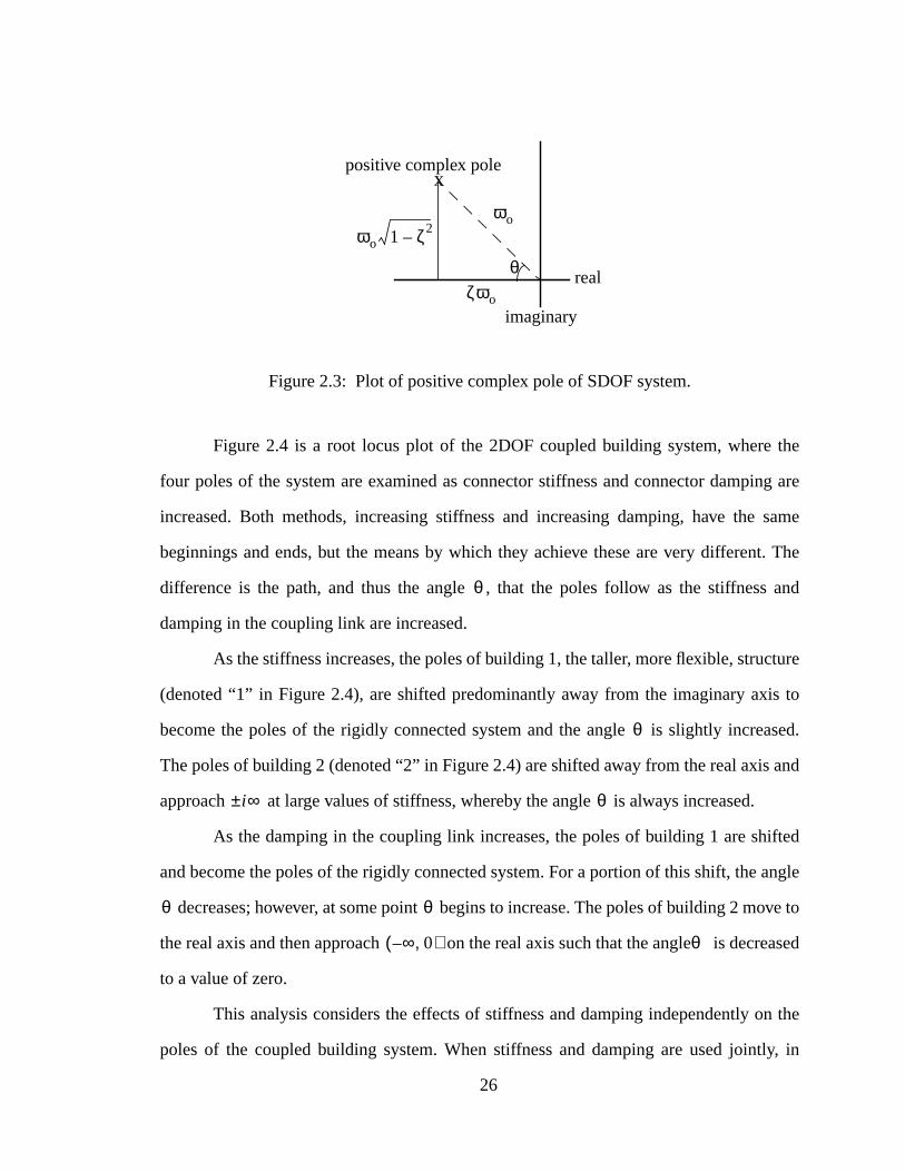
As part of this analysis, first consider the characteristic equation of a SDOF
tem, , and the corresponding poles
Sketching the positive complex pole, as in Figure 2.3, the angle is observed to be re
to the damping of the SDOF system by . For more critical values of damp
( ), the angle approaches zero. Thus, the smaller the angle , the more damp
present in the SDOF system. The angle is a good measure of system damping.
Φ t τ,( ) eA t τ–( )
= z 0( )
s2
2ζωos ωo2
+ + 0= s ζ– ωo jωo 1 ζ2–±=
θ
θcos ζ=
ζ 1→ θ θ
θ
25
the
ng are
same
t. The
and
ture
s to
ased.
and
.
fted
angle
ove to
eased
n the
ly, in
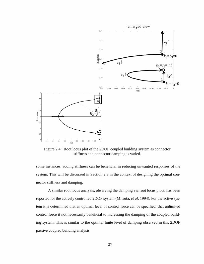
Figure 2.4 is a root locus plot of the 2DOF coupled building system, where
four poles of the system are examined as connector stiffness and connector dampi
increased. Both methods, increasing stiffness and increasing damping, have the
beginnings and ends, but the means by which they achieve these are very differen
difference is the path, and thus the angle , that the poles follow as the stiffness
damping in the coupling link are increased.
As the stiffness increases, the poles of building 1, the taller, more flexible, struc
(denoted “1” in Figure 2.4), are shifted predominantly away from the imaginary axi
become the poles of the rigidly connected system and the angle is slightly incre
The poles of building 2 (denoted “2” in Figure 2.4) are shifted away from the real axis
approach at large values of stiffness, whereby the angle is always increased
As the damping in the coupling link increases, the poles of building 1 are shi
and become the poles of the rigidly connected system. For a portion of this shift, the
decreases; however, at some point begins to increase. The poles of building 2 m
the real axis and then approach on the real axis such that the angle is decr
to a value of zero.
This analysis considers the effects of stiffness and damping independently o
poles of the coupled building system. When stiffness and damping are used joint
Figure 2.3: Plot of positive complex pole of SDOF system.
real
imaginary
x
ζωo
ωo 1 ζ2–
ωo
θ
positive complex pole
θ
θ
i∞± θ
θ θ
∞– 0,( ) θ
26
of the
con-
een
ited
uild-
OF
some instances, adding stiffness can be beneficial in reducing unwanted responses
system. This will be discussed in Section 2.3 in the context of designing the optimal
nector stiffness and damping.
A similar root locus analysis, observing the damping via root locus plots, has b
reported for the actively controlled 2DOF system (Mitsuta,et al. 1994). For the active sys-
tem it is determined that an optimal level of control force can be specified, that unlim
control force it not necessarily beneficial to increasing the damping of the coupled b
ing system. This is similar to the optimal finite level of damping observed in this 2D
passive coupled building analysis.
−2 −1.8 −1.6 −1.4 −1.2 −1 −0.8 −0.6 −0.4 −0.2 0−2
−1.5
−1
−0.5
0
0.5
1
1.5
2
imag
inar
y
real
−0.2 −0.18 −0.16 −0.14 −0.12 −0.1 −0.08 −0.06 −0.04 −0.02 01.2
1.3
1.4
1.5
1.6
1.7
1.8
imag
inar
y
real
Figure 2.4: Root locus plot of the 2DOF coupled building system as connectorstiffness and connector damping is varied.
enlarged view
k3=c3=0
k3=c3=0
k3=c3=inf
k3^
k3^
c3^
c3^
θ2θ1
2
1
27
s of
in an
m an
of the
e two
.5.
oth
mono-
the
ver, as
asing
m the
l fre-
al fre-
nt of
ini-
onant
d sys-
shift-
f the
tent,
een
2DOF Coupled Building Transfer Function Analysis
A transfer function analysis can provide further insight into the modal response
each structure as the parameters of the coupling link are varied. From the worst case
sense, minimizing the resonant peaks of the transfer function are of interest. Fro
sense, the area under the transfer function is of interest. The transfer functions
ground acceleration to the displacement, velocity and absolute acceleration of th
buildings as the connector stiffness and damping is varied are presented in Figure 2
As the stiffness in the coupling link is increased the natural frequencies of b
buildings increase. The difference between the two frequencies does not increase
tonically for all values of the stiffness. In particular, for small stiffness increases in
coupling member, the first natural frequency increases faster than the second. Howe
the stiffness becomes larger, the difference does increase monotonically. The incre
frequencies were observed in the root locus analysis with the poles moving away fro
origin. The first natural frequency tends to a value between the two uncoupled natura
quencies (the natural frequency of the rigidly connected system). The second natur
quency continues to get very large, eventually above the significant frequency conte
the ground excitation.
As the damping in the coupling link is increased, the natural frequencies are
tially observed to increase. As the buildings become more coupled, one of the res
peaks dampens out, until only one resonant peak is observed for the rigidly connecte
tem. The increase in damping was examined in the root locus analysis with one pole
ing towards the real axis and becoming critically damped.
Increasing the stiffness has the effect of increasing the natural frequencies o
system. While this may be a valid technique to avoid inputs with a narrow energy con
this type of control may not be valid for seismic inputs with wide energy spectrums s
historically, and especially not for the white noise excitation assumed here.
H∞
H2
28
ityd.
0 0.05 0.1 0.15 0.2 0.25 0.3 0.35 0.4 0.45 0.5−30
−20
−10
0
10
20
30
mag
nitu
de (
dB)
frequency (Hz)
Building 1Building 2Rigid Connection
0 0.05 0.1 0.15 0.2 0.25 0.3 0.35 0.4 0.45 0.5−30
−20
−10
0
10
20
30
mag
nitu
de (
dB)
frequency (Hz)
0 0.05 0.1 0.15 0.2 0.25 0.3 0.35 0.4 0.45 0.5−30
−20
−10
0
10
20
30
mag
nitu
de (
dB)
frequency (Hz)
0 0.05 0.1 0.15 0.2 0.25 0.3 0.35 0.4 0.45 0.5−30
−20
−10
0
10
20
30
mag
nitu
de (
dB)
frequency (Hz)
Building 1Building 2Rigid Connection
0 0.05 0.1 0.15 0.2 0.25 0.3 0.35 0.4 0.45 0.5−30
−20
−10
0
10
20
30
mag
nitu
de (
dB)
frequency (Hz)
0 0.05 0.1 0.15 0.2 0.25 0.3 0.35 0.4 0.45 0.5−30
−20
−10
0
10
20
30
mag
nitu
de (
dB)
frequency (Hz)
Figure 2.5: Transfer function from the ground acceleration to displacement, velocand absolute acceleration as connector stiffness and connector damping is varie
Hx1xgω( ) Hx1xg
ω( )
Hx1xgω( ) Hx2xg
ω( )
Hx1
axg
ω( ) Hx2
axg
ω( )
vary stiffness
vary stiffness
vary stiffness vary damping
vary damping
vary damping
29
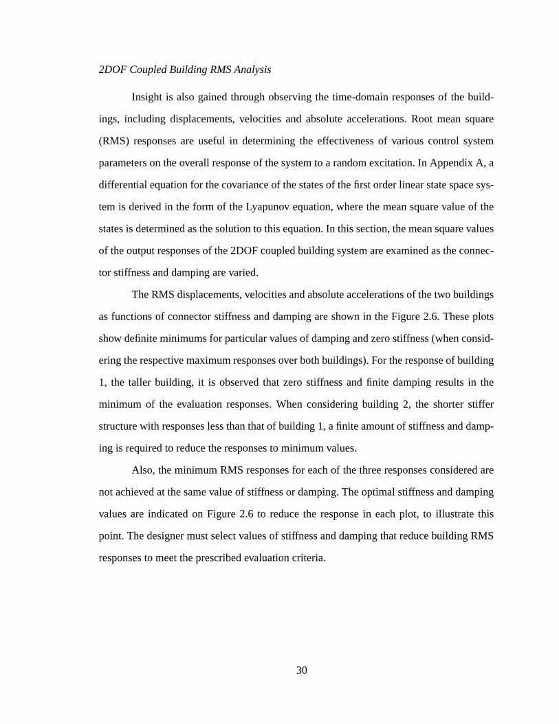
uild-
quare
stem
x A, a
e sys-
f the
values
nnec-
ings
plots
nsid-
ilding
the
tiffer
amp-
d are
ping
e this
RMS
2DOF Coupled Building RMS Analysis
Insight is also gained through observing the time-domain responses of the b
ings, including displacements, velocities and absolute accelerations. Root mean s
(RMS) responses are useful in determining the effectiveness of various control sy
parameters on the overall response of the system to a random excitation. In Appendi
differential equation for the covariance of the states of the first order linear state spac
tem is derived in the form of the Lyapunov equation, where the mean square value o
states is determined as the solution to this equation. In this section, the mean square
of the output responses of the 2DOF coupled building system are examined as the co
tor stiffness and damping are varied.
The RMS displacements, velocities and absolute accelerations of the two build
as functions of connector stiffness and damping are shown in the Figure 2.6. These
show definite minimums for particular values of damping and zero stiffness (when co
ering the respective maximum responses over both buildings). For the response of bu
1, the taller building, it is observed that zero stiffness and finite damping results in
minimum of the evaluation responses. When considering building 2, the shorter s
structure with responses less than that of building 1, a finite amount of stiffness and d
ing is required to reduce the responses to minimum values.
Also, the minimum RMS responses for each of the three responses considere
not achieved at the same value of stiffness or damping. The optimal stiffness and dam
values are indicated on Figure 2.6 to reduce the response in each plot, to illustrat
point. The designer must select values of stiffness and damping that reduce building
responses to meet the prescribed evaluation criteria.
30
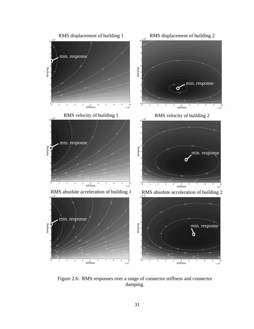
r
0 1 2 3 4 5 6 7 8 9 10
x 106
0
1
2
3
4
5
6
7
8
9
10x 10
6
stiffness
dam
ping
5
5
5.5
5.5
5.5
6
6
6
6
6.5
6.5
6.5
7
7
7
7
7.5
7.5
7.5
7
88
8
8.58.5 8.5
0 1 2 3 4 5 6 7 8 9 10
x 106
0
1
2
3
4
5
6
7
8
9
10x 10
6
stiffness
dam
ping
6.5
7
7
7
7.5
7.5
7.5
8
8
8
8
8.5
8.5
8.5
9
9
9
9
9.5
9.5
9.5
9.5
10
10
10
10
10.510.5
10.5
1111
11
11 5 11.5
0 1 2 3 4 5 6 7 8 9 10
x 106
0
1
2
3
4
5
6
7
8
9
10x 10
6
stiffness
dam
ping
3.5
3.5
4
4
4
4
4
4
4
4.5
4.54.5
4.5
55.5
0 1 2 3 4 5 6 7 8 9 10
x 106
0
1
2
3
4
5
6
7
8
9
10x 10
6
stiffness
dam
ping
5.5
5.55.5
5.5
5.5
5.5
6
6
6
6
66
6
6.6.56.5
6.5
77
7
7 588.59
0 1 2 3 4 5 6 7 8 9 10
x 106
0
1
2
3
4
5
6
7
8
9
10x 10
6
stiffness
dam
ping
9
9
9.5
9.5
9.5
10
10
10
10.5
10.5
10.5
10.5
11
11
11
11
11.5
11.5
11.5
11.512
12
12
12
12.5
12.5
12.5
12
13
13
13
13.5
13.5
13.5
14
14
14
14.514.5
14.5
1515
15 50 1 2 3 4 5 6 7 8 9 10
x 106
0
1
2
3
4
5
6
7
8
9
10x 10
6
stiffness
dam
ping
8
88
8
8
8
8.5
8.5
8.5 8.5
8.58.5
8.5
9
99
99.5
9.59.5 9.5
10
1010 10
10.5
10.510.511
1111.5
11.5
12
1212.51313.514
Figure 2.6: RMS responses over a range of connector stiffness and connectodamping.
RMS displacement of building 1 RMS displacement of building 2
RMS velocity of building 1 RMS velocity of building 2
RMS absolute acceleration of building 2RMS absolute acceleration of building 1
min. response
min. response
min. response
min. response
min. responsemin. response
31
the
n, the
and
l pas-
pled
, the
ined.
opti-
mped
nami,
nite)
sys-
at the
ctor
een in
nnec-
sed to
m are
higher
e con-
2.3 2DOF Coupled Building Optimal Passive Control Strategy
Previously, the effects of varying the connector stiffness and damping on
eigenvalues, transfer functions, and RMS responses were considered. In this sectio
optimal passive design will be discussed. Now that the effect of the coupling stiffness
damping on the coupled building system is known, consider the design of the optima
sive system for the two SDOF building models. First consider an undamped cou
building system and the P and Q theory to design the optimal connector link. Next
more complex damped coupled building optimum coupling link parameters are exam
Undamped Coupled Building System
For the undamped coupled building system, P, Q theory is used to design the
mal passive controller to reduce the resonant peaks (Seto, 1998). For three unda
SDOF structures, the method of P, Q theory has been extended to P, T, Q theory (Iwa
et al. 1986). Neither the zero connector stiffness and damping, the maximum (infi
connector stiffness or the maximum (infinite) connector damping produce optimal
tems. Neither result in systems with any damping. The responses are unbounded
natural frequencies, which is highly undesirable. The optimal values for the conne
stiffness and damping are somewhere between zero and infinity. This trend was s
previous root locus, transfer function, and RMS response analyses. As before, the co
tor stiffness is used to vary the natural frequencies and the connector damping is u
vary the magnitude of the transfer function.
When the connector stiffness is increased, the natural frequencies of the syste
also increased, beginning at the uncoupled natural frequencies and approaching the
fused natural frequencies. The bounds for the natural frequencies of the system as th
32
are
ction
ds for
n the
d Q,
the
f the
P and
g (for
nt Q
, the
oint P,
ed by
agni-
equal
iscus-
nnot
ariant
d by
nsfer
io of
ent to
very
nector stiffness is varied, and damping set to zero,
and .
When the connector damping is increased, the magnitude of the transfer fun
at the resonant peaks, frequencies and , decreases. The boun
the magnitude of the transfer function as the connector damping is varied lie betwee
magnitude of the undamped and the fused transfer functions.
The method of the theory of P, Q requires observing two points, called P an
that are the intersection of the transfer functions of the two uncoupled buildings with
transfer function of the rigidly connected coupled building system. As the stiffness o
connector is changed, the locations of P and Q are varied and thus the magnitude of
Q are varied. The points P and Q, however, remain invariant to the connector dampin
the undamped buildings). When the stiffness is zero, point P is higher than poi
( ) for the displacement responses. As the stiffness is increased
magnitude of point P is increased and the magnitude of point Q is decreased. So p
when considering displacements, is the larger magnitude point and can not be reduc
increasing stiffness. When considering absolute accelerations, point Q is of larger m
tude, thus increasing the connector stiffness can bring down Q, while raising P, to
magnitudes. However, P, Q theory is defined with respect to displacements, so the d
sion regarding absolute accelerations will be given in subsequent sections.
The magnitude of the transfer function at the frequencies of points P and Q ca
be reduced by varying the damping. As was previously stated, points P and Q are inv
to connector damping. The magnitude at all other points can be significantly reduce
varying the connector damping such that point P, or point Q, is a maximum on the tra
function curve.
Seto (1998) has developed the analytical solutions for the optimal damping rat
the connector to reduce the resonant peaks of the transfer functions of displacem
ground excitation. The P, Q theory developed for the coupled building problem is
ωo1 ω1 k3 0,( ) k1 k2+( ) m1 m2+( )⁄≤ ≤ ωo2 ω2 k3 0,( ) ∞≤ ≤
ω1 k3 c3,( ) ω2 k3 c3,( )
magP 0( ) magQ 0( )>
33
ent
mass
st be
encies
ed, in
dis-
ce
y in
2.1,
y set
iated
from
specifically defined and somewhat restrictive in that it is limited to reducing displacem
responses, reducing the norm of the transfer function, and requiring a specific
and frequency ratio of the two buildings.
The P, Q theory requires first, an optimal mass and stiffness relationship mu
determined to insure that points P and Q are of equal heights. Here, the natural frequ
should be fixed, and the masses will be varied. The optimal mass ratio is thus defin
terms of the natural frequencies, as
(2.7)
Seto’s closed form optimal damping ratio, to reduce the resonant peak of the
placement transfer function of building 1 or of building 2, are as follows:
or (2.8)
where is the optimal damping ratio of the coupling link to redu
the peak of the displacement transfer function of the ith building to ground acceleration.
Undamped Coupled Building System Numerical Example
Consider the mass and stiffness of the building 1, as defined previousl
Table 2.1. Assume also, the frequency of building 2 remains the same as in Table
0.247 Hz. The new mass and stiffness of building 2, from Equation (2.7), are optimall
to kg and N/m.
For the 2DOF building system considered in this dissertation, with no assoc
structural damping, the optimal connector stiffness is zero and the optimal damping,
Equation (2.8), to reduce the peak of the displacement transfer functions are
H∞
µm2
m1------
ωo1
ωo2---------= =
ζopt1 4– 4µ 3µ2
– 2µ3– µ4
–+
8µ 1 3µ 3µ2 µ3+ + +( )
---------------------------------------------------------------= ζopt2 1 2µ 3µ2
– 4µ3– 4µ4
+ +
8µ 1 3µ 3µ2 µ3+ + +( )
--------------------------------------------------------------=
ζopti
c3 2 k2m2( )⁄=
m2 2.23667×10= k2 7.1460
7×10=
34
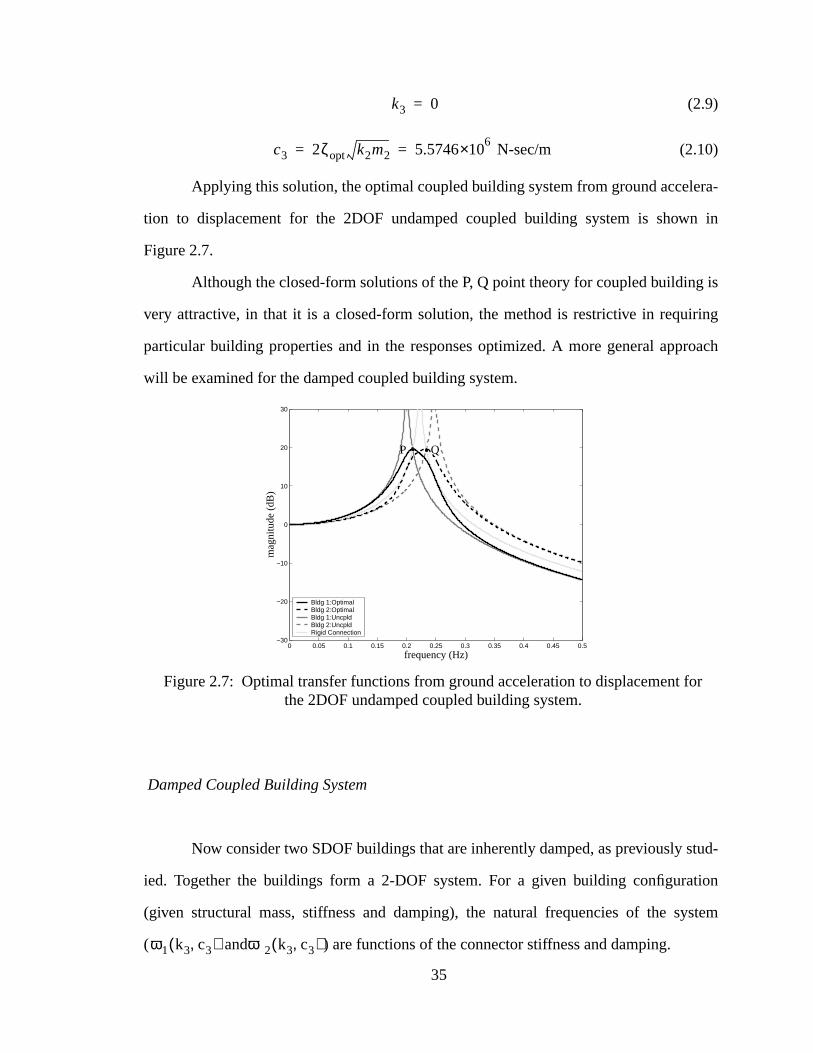
ra-
n in
is
ring
roach
tud-
tion
stem
or
(2.9)
N-sec/m (2.10)
Applying this solution, the optimal coupled building system from ground accele
tion to displacement for the 2DOF undamped coupled building system is show
Figure 2.7.
Although the closed-form solutions of the P, Q point theory for coupled building
very attractive, in that it is a closed-form solution, the method is restrictive in requi
particular building properties and in the responses optimized. A more general app
will be examined for the damped coupled building system.
Damped Coupled Building System
Now consider two SDOF buildings that are inherently damped, as previously s
ied. Together the buildings form a 2-DOF system. For a given building configura
(given structural mass, stiffness and damping), the natural frequencies of the sy
( and ) are functions of the connector stiffness and damping.
k3 0=
c3 2ζopt k2m2 5.57466×10= =
0 0.05 0.1 0.15 0.2 0.25 0.3 0.35 0.4 0.45 0.5−30
−20
−10
0
10
20
30
mag
nitu
de (
dB)
frequency (Hz)
Bldg 1:Optimal Bldg 2:Optimal Bldg 1:Uncpld Bldg 2:Uncpld Rigid Connection
Figure 2.7: Optimal transfer functions from ground acceleration to displacement fthe 2DOF undamped coupled building system.
QP
ω1 k3 c3,( ) ω2 k3 c3,( )
35
m are
higher
sys-
the
ction
ound
. The
d lie
tions.
is not
sys-
d and
Q no
. The
nnec-
nd Q,
nger
opti-
Algo-
When the connector stiffness is increased, the natural frequencies of the syste
also increased, beginning at the uncoupled natural frequencies and approaching the
rigidly connected natural frequencies. The bounds for the natural frequencies of the
tem as the connector stiffness is
(2.11)
where the undamped natural frequency of building 1 is and
undamped natural frequency of building 2 is .
When the connector damping is increased the magnitude of the transfer fun
(in this case the transfer function of the absolute acceleration of the building to a gr
excitation) at the resonant peaks, frequencies and , decreases
bounds for the magnitude of the transfer function as the connector damping is varie
between the magnitude of the undamped and the rigidly connected transfer func
Connector damping does affect the natural frequencies of the system, but the effect
so dramatic, and thus not focused on in attempting to understand this process.
Again points P and Q can be observed, as in the undamped coupled building
tem. As the stiffness of the connector is changed, the locations of P and Q are varie
thus the magnitude of P and Q are varied. Important to note is that the points P and
longer remain invariant to the connector damping for the case of the damped building
magnitude of points P and Q are functions of both the connector stiffness and the co
tor damping. Again, damping does not have a dramatic effect on the placement of P a
however, it does effect the magnitude of the transfer functions.
The method of theory of P, Q can not be applied here, as P and Q are no lo
invariant to connector damping. For damped structures other methods to determine
mal connector stiffness and damping values have been considered including Genetic
ωo1 1 ζ12
–( ) ω1 k3 c3,( ) k1 k2+( ) m1 m2+( )⁄[ ] 1 ζ12
–( )≤ ≤
ωo2 1 ζ22
–( ) ω2 k3 c3,( ) ∞≤ ≤
ωo1 k1 m1⁄=
ωo2 k2 m2⁄=
ω1 k3 c3,( ) ω2 k3 c3,( )
36
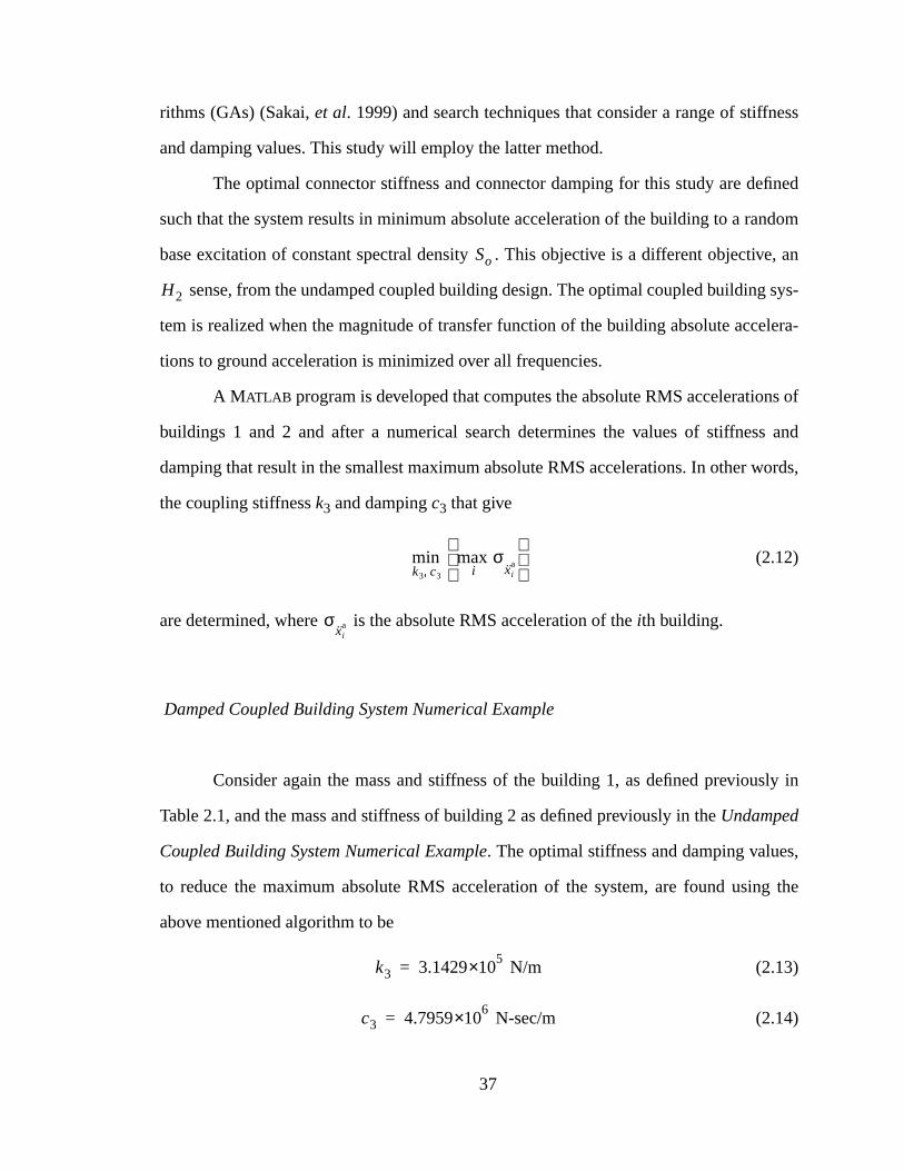
ess
fined
ndom
e, an
sys-
lera-
ns of
s and
ords,
ly in
s,
g the
rithms (GAs) (Sakai,et al. 1999) and search techniques that consider a range of stiffn
and damping values. This study will employ the latter method.
The optimal connector stiffness and connector damping for this study are de
such that the system results in minimum absolute acceleration of the building to a ra
base excitation of constant spectral density . This objective is a different objectiv
sense, from the undamped coupled building design. The optimal coupled building
tem is realized when the magnitude of transfer function of the building absolute acce
tions to ground acceleration is minimized over all frequencies.
A MATLAB program is developed that computes the absolute RMS acceleratio
buildings 1 and 2 and after a numerical search determines the values of stiffnes
damping that result in the smallest maximum absolute RMS accelerations. In other w
the coupling stiffnessk3 and dampingc3 that give
(2.12)
are determined, where is the absolute RMS acceleration of theith building.
Damped Coupled Building System Numerical Example
Consider again the mass and stiffness of the building 1, as defined previous
Table 2.1, and the mass and stiffness of building 2 as defined previously in theUndamped
Coupled Building System Numerical Example. The optimal stiffness and damping value
to reduce the maximum absolute RMS acceleration of the system, are found usin
above mentioned algorithm to be
N/m (2.13)
N-sec/m (2.14)
So
H2
mink3 c3,
maxi
σxi
a
σxi
a
k3 3.14295×10=
c3 4.79596×10=
37
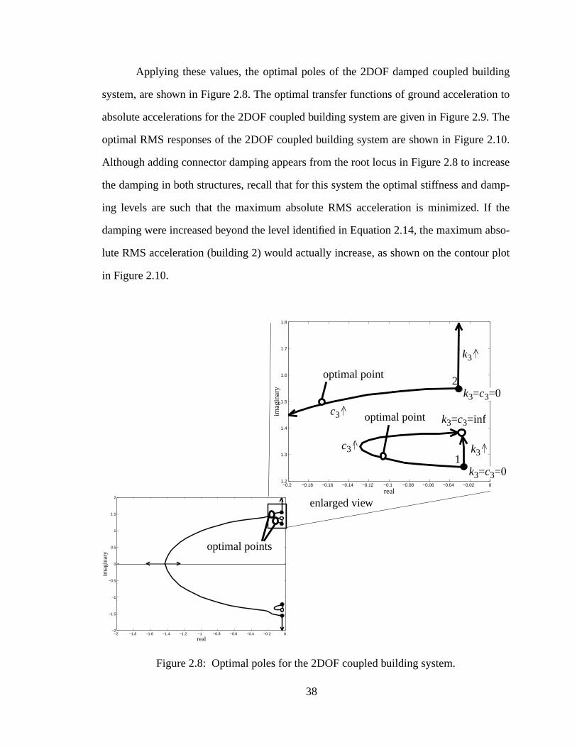
ding
on to
. The
2.10.
rease
amp-
f the
abso-
plot
Applying these values, the optimal poles of the 2DOF damped coupled buil
system, are shown in Figure 2.8. The optimal transfer functions of ground accelerati
absolute accelerations for the 2DOF coupled building system are given in Figure 2.9
optimal RMS responses of the 2DOF coupled building system are shown in Figure
Although adding connector damping appears from the root locus in Figure 2.8 to inc
the damping in both structures, recall that for this system the optimal stiffness and d
ing levels are such that the maximum absolute RMS acceleration is minimized. I
damping were increased beyond the level identified in Equation 2.14, the maximum
lute RMS acceleration (building 2) would actually increase, as shown on the contour
in Figure 2.10.
Figure 2.8: Optimal poles for the 2DOF coupled building system.
−2 −1.8 −1.6 −1.4 −1.2 −1 −0.8 −0.6 −0.4 −0.2 0−2
−1.5
−1
−0.5
0
0.5
1
1.5
2
imag
inar
y
real
−0.2 −0.18 −0.16 −0.14 −0.12 −0.1 −0.08 −0.06 −0.04 −0.02 01.2
1.3
1.4
1.5
1.6
1.7
1.8
imag
inar
y
real
enlarged view
k3=c3=0
k3=c3=0
k3=c3=inf
k3^
k3^
c3^
c3^
2
1
optimal point
optimal point
optimal points
38
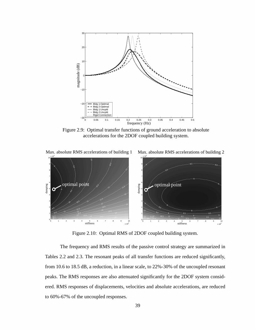
ed in
antly,
nant
onsid-
educed
2
The frequency and RMS results of the passive control strategy are summariz
Tables 2.2 and 2.3. The resonant peaks of all transfer functions are reduced signific
from 10.6 to 18.5 dB, a reduction, in a linear scale, to 22%-30% of the uncoupled reso
peaks. The RMS responses are also attenuated significantly for the 2DOF system c
ered. RMS responses of displacements, velocities and absolute accelerations, are r
to 60%-67% of the uncoupled responses.
0 0.05 0.1 0.15 0.2 0.25 0.3 0.35 0.4 0.45 0.5−30
−20
−10
0
10
20
30
mag
nitu
de (
dB)
frequency (Hz)
Bldg 1:Optimal Bldg 2:Optimal Bldg 1:Uncpld Bldg 2:Uncpld Rigid Connection
Figure 2.9: Optimal transfer functions of ground acceleration to absoluteaccelerations for the 2DOF coupled building system.
0 1 2 3 4 5 6 7 8 9 10
x 106
0
1
2
3
4
5
6
7
8
9
10x 10
6
stiffness
dam
ping
9
9
9.5
9.5
9.5
10
10
10
10.5
10.5
10.5
10.5 11
11
11
11
11.5
11.5
11.5
11.5
12
12
12
12
12.5
12.5
12.5
13
13
13
13
13.5
13.5
13.5
14
14
14
14.514.5
1515
15 50 1 2 3 4 5 6 7 8 9 10
x 106
0
1
2
3
4
5
6
7
8
9
10x 10
6
stiffness
dam
ping
8
8
8
8
8
8
8.58.5
8.5
8.5
8.5
8.5 8.5
9
9
99 9
9.5
9.5 9.5
10
1010 10
10.510.5 10.511
11
11 5
11.512
1212.51313.514
Figure 2.10: Optimal RMS of 2DOF coupled building system.
Max. absolute RMS accelerations of building 1Max. absolute RMS accelerations of building
optimal point optimal point
39
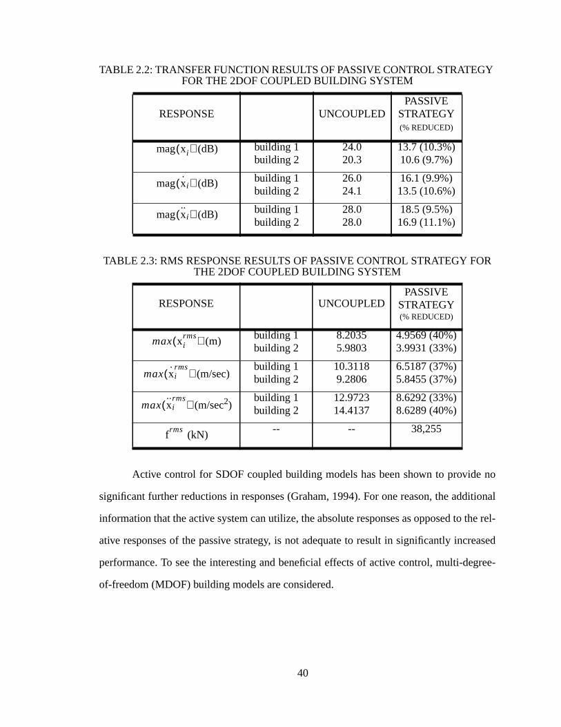
no
itional
the rel-
eased
gree-
R
Active control for SDOF coupled building models has been shown to provide
significant further reductions in responses (Graham, 1994). For one reason, the add
information that the active system can utilize, the absolute responses as opposed to
ative responses of the passive strategy, is not adequate to result in significantly incr
performance. To see the interesting and beneficial effects of active control, multi-de
of-freedom (MDOF) building models are considered.
TABLE 2.2: TRANSFER FUNCTION RESULTS OF PASSIVE CONTROL STRATEGYFOR THE 2DOF COUPLED BUILDING SYSTEM
RESPONSE UNCOUPLEDPASSIVE
STRATEGY(% REDUCED)
(dB) building 1building 2
24.020.3
13.7 (10.3%)10.6 (9.7%)
(dB) building 1building 2
26.024.1
16.1 (9.9%)13.5 (10.6%)
(dB) building 1building 2
28.028.0
18.5 (9.5%)16.9 (11.1%)
TABLE 2.3: RMS RESPONSE RESULTS OF PASSIVE CONTROL STRATEGY FOTHE 2DOF COUPLED BUILDING SYSTEM
RESPONSE UNCOUPLEDPASSIVE
STRATEGY(% REDUCED)
(m) building 1building 2
8.20355.9803
4.9569 (40%)3.9931 (33%)
(m/sec)building 1building 2
10.31189.2806
6.5187 (37%)5.8455 (37%)
(m/sec2)building 1building 2
12.972314.4137
8.6292 (33%)8.6289 (40%)
(kN) -- -- 38,255
mag xi( )
mag xi( )
mag xi( )
max xirms( )
max xirms
( )
max xirms
( )
frms
40
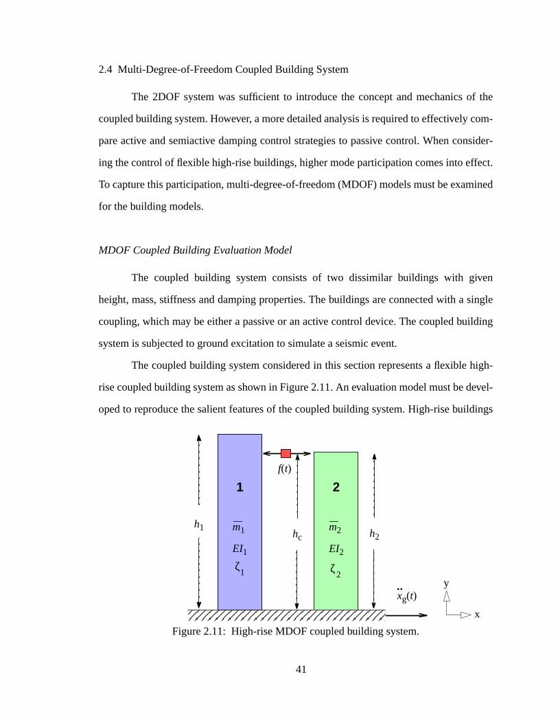
f the
com-
sider-
ect.
ined
en
single
lding
high-
evel-
dings
2.4 Multi-Degree-of-Freedom Coupled Building System
The 2DOF system was sufficient to introduce the concept and mechanics o
coupled building system. However, a more detailed analysis is required to effectively
pare active and semiactive damping control strategies to passive control. When con
ing the control of flexible high-rise buildings, higher mode participation comes into eff
To capture this participation, multi-degree-of-freedom (MDOF) models must be exam
for the building models.
MDOF Coupled Building Evaluation Model
The coupled building system consists of two dissimilar buildings with giv
height, mass, stiffness and damping properties. The buildings are connected with a
coupling, which may be either a passive or an active control device. The coupled bui
system is subjected to ground excitation to simulate a seismic event.
The coupled building system considered in this section represents a flexible
rise coupled building system as shown in Figure 2.11. An evaluation model must be d
oped to reproduce the salient features of the coupled building system. High-rise buil
..
1 2
h2h1 m2m1
f(t)
xg(t)
EI1 EI2
Figure 2.11: High-rise MDOF coupled building system.
ζ1 ζ
2
x
y
hc
41
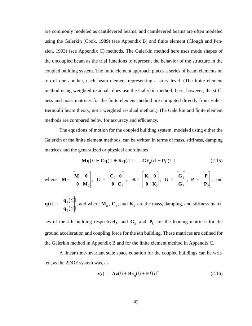
odeled
Pen-
pes of
in the
nts on
ment
stiff-
uler-
ment
r the
ping
atri-
the
r
.
writ-
are commonly modeled as cantilevered beams, and cantilevered beams are often m
using the Galerkin (Cook, 1989) (see Appendix B) and finite element (Clough and
zien, 1993) (see Appendix C) methods. The Galerkin method here uses mode sha
the uncoupled beam as the trial functions to represent the behavior of the structure
coupled building system. The finite element approach places a series of beam eleme
top of one another, each beam element representing a story level. (The finite ele
method using weighted residuals does use the Galerkin method; here, however, the
ness and mass matrices for the finite element method are computed directly from E
Bernoulli beam theory, not a weighted residual method.) The Galerkin and finite ele
methods are compared below for accuracy and efficiency.
The equations of motion for the coupled building system, modeled using eithe
Galerkin or the finite element methods, can be written in terms of mass, stiffness, dam
matrices and the generalized or physical coordinates
(2.15)
where , , , , , and
, and where , , and are the mass, damping, and stiffness m
ces of thekth building respectively, and and are the loading matrices for
ground acceleration and coupling force for thekth building. These matrices are defined fo
the Galerkin method in Appendix B and for the finite element method in Appendix C
A linear time-invariant state space equation for the coupled buildings can be
ten, as the 2DOF system was, as
(2.16)
Mq t( ) Cq t( ) Kq t( )+ + G xg t( )– Pf t( )+=
MM 1 0
0 M2
= CC1 0
0 C2
= KK1 0
0 K2
= GG1
G2
= PP1
P2
=
q t( )q1 t( )
q2 t( )= M k Ck K k
Gk Pk
z t( ) Az t( ) B xg t( ) Ef t( )+ +=
42
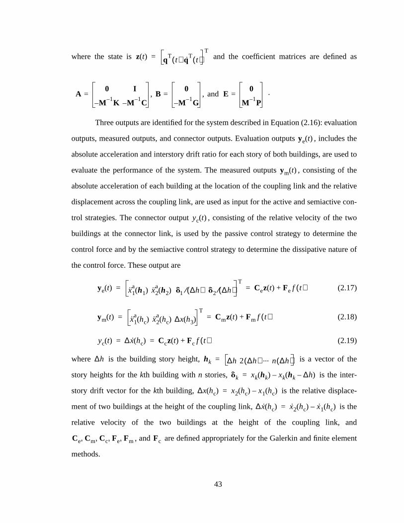
as
ation
es the
ed to
of the
ative
e con-
two
e the
re of
e
e
nd
ent
where the state is and the coefficient matrices are defined
.
Three outputs are identified for the system described in Equation (2.16): evalu
outputs, measured outputs, and connector outputs. Evaluation outputs , includ
absolute acceleration and interstory drift ratio for each story of both buildings, are us
evaluate the performance of the system. The measured outputs , consisting
absolute acceleration of each building at the location of the coupling link and the rel
displacement across the coupling link, are used as input for the active and semiactiv
trol strategies. The connector output , consisting of the relative velocity of the
buildings at the connector link, is used by the passive control strategy to determin
control force and by the semiactive control strategy to determine the dissipative natu
the control force. These output are
(2.17)
(2.18)
(2.19)
where is the building story height, is a vector of th
story heights for thekth building with n stories, is the inter-
story drift vector for thekth building, is the relative displace-
ment of two buildings at the height of the coupling link, is th
relative velocity of the two buildings at the height of the coupling link, a
, and are defined appropriately for the Galerkin and finite elem
methods.
z t( ) qTt( ) qT
t( )T
=
A0 I
M–1– K M–
1– C,= B
0
M 1– G–,= and E
0
M 1– P=
ye t( )
ym t( )
yc t( )
ye t( ) x1a h1( ) x2
a h2( ) d1 ∆h( )⁄ d2 ∆h( )⁄T
Cez t( ) Fe f t( )+= =
ym t( ) x1a
hc( ) x2a
hc( ) ∆x h3( )T
Cmz t( ) Fm f t( )+= =
yc t( ) ∆ x hc( ) Ccz t( ) Fc f t( )+= =
∆h hk ∆h 2 ∆h( ) ... n ∆h( )=
dk xk hk( ) xk hk ∆h–( )–=
∆x hc( ) x2 hc( ) x1 hc( )–=
∆ x hc( ) x2 hc( ) x1 hc( )–=
Ce Cm Cc Fe Fm, , , , Fc
43
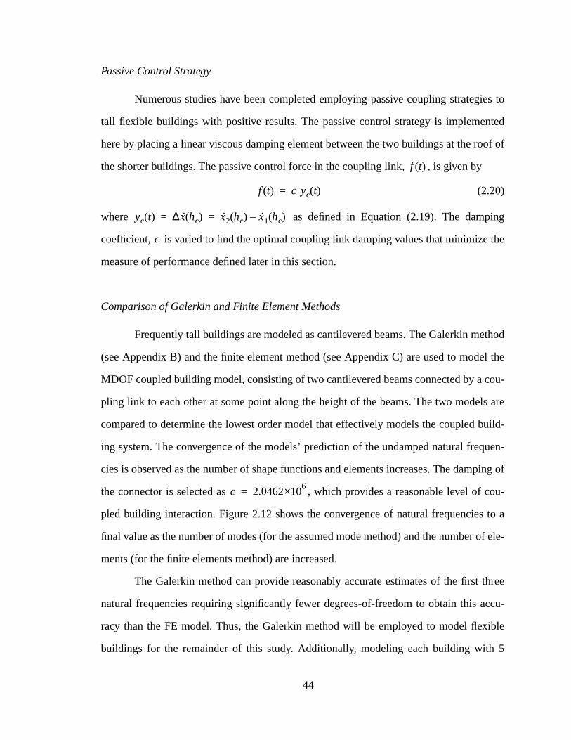
ies to
ted
of of
ng
the
thod
el the
cou-
ls are
uild-
quen-
ping of
cou-
to a
of ele-
three
ccu-
ible
5
Passive Control Strategy
Numerous studies have been completed employing passive coupling strateg
tall flexible buildings with positive results. The passive control strategy is implemen
here by placing a linear viscous damping element between the two buildings at the ro
the shorter buildings. The passive control force in the coupling link, , is given by
(2.20)
where as defined in Equation (2.19). The dampi
coefficient, is varied to find the optimal coupling link damping values that minimize
measure of performance defined later in this section.
Comparison of Galerkin and Finite Element Methods
Frequently tall buildings are modeled as cantilevered beams. The Galerkin me
(see Appendix B) and the finite element method (see Appendix C) are used to mod
MDOF coupled building model, consisting of two cantilevered beams connected by a
pling link to each other at some point along the height of the beams. The two mode
compared to determine the lowest order model that effectively models the coupled b
ing system. The convergence of the models’ prediction of the undamped natural fre
cies is observed as the number of shape functions and elements increases. The dam
the connector is selected as , which provides a reasonable level of
pled building interaction. Figure 2.12 shows the convergence of natural frequencies
final value as the number of modes (for the assumed mode method) and the number
ments (for the finite elements method) are increased.
The Galerkin method can provide reasonably accurate estimates of the first
natural frequencies requiring significantly fewer degrees-of-freedom to obtain this a
racy than the FE model. Thus, the Galerkin method will be employed to model flex
buildings for the remainder of this study. Additionally, modeling each building with
f t( )
f t( ) c yc t( )=
yc t( ) ∆ x hc( ) x2 hc( ) x1 hc( )–= =
c
c 2.04626×10=
44
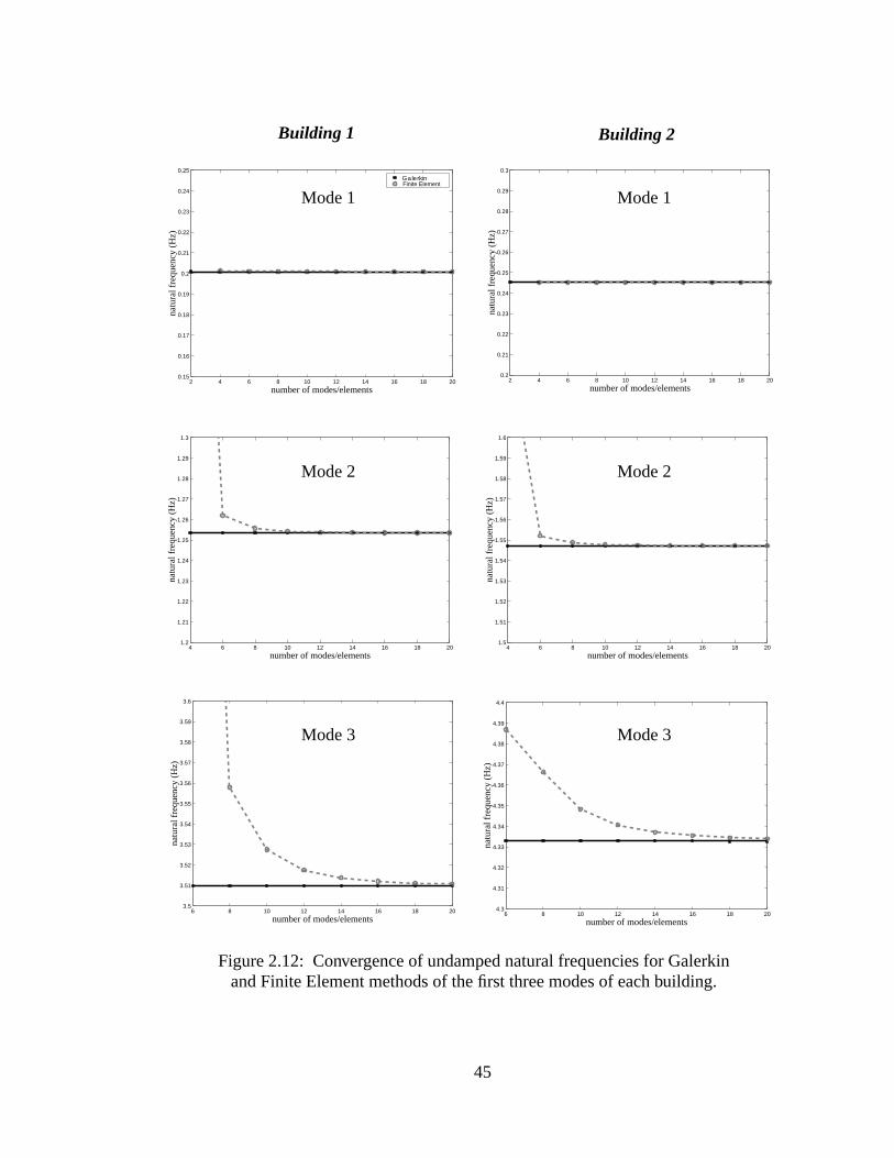
2 4 6 8 10 12 14 16 18 200.15
0.16
0.17
0.18
0.19
0.2
0.21
0.22
0.23
0.24
0.25na
tura
l fre
quen
cy (
Hz)
number of modes/elements
Assumed Modes Finite Element
2 4 6 8 10 12 14 16 18 200.2
0.21
0.22
0.23
0.24
0.25
0.26
0.27
0.28
0.29
0.3
natu
ral f
requ
ency
(H
z)
number of modes/elements
4 6 8 10 12 14 16 18 201.2
1.21
1.22
1.23
1.24
1.25
1.26
1.27
1.28
1.29
1.3
natu
ral f
requ
ency
(H
z)
number of modes/elements4 6 8 10 12 14 16 18 20
1.5
1.51
1.52
1.53
1.54
1.55
1.56
1.57
1.58
1.59
1.6
natu
ral f
requ
ency
(H
z)
number of modes/elements
6 8 10 12 14 16 18 203.5
3.51
3.52
3.53
3.54
3.55
3.56
3.57
3.58
3.59
3.6
natu
ral f
requ
ency
(H
z)
number of modes/elements6 8 10 12 14 16 18 20
4.3
4.31
4.32
4.33
4.34
4.35
4.36
4.37
4.38
4.39
4.4
natu
ral f
requ
ency
(H
z)
number of modes/elements
Figure 2.12: Convergence of undamped natural frequencies for Galerkinand Finite Element methods of the first three modes of each building.
Mode 1 Mode 1
Mode 2 Mode 2
Mode 3 Mode 3
Building 1 Building 2
Galerkin
45
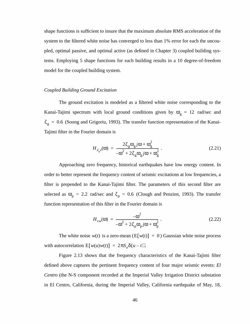
of the
ncou-
sys-
dom
the
nd
nai-
t. In
ies, a
are
nsfer
ess
lter
ts:
tion
8,
shape functions is sufficient to insure that the maximum absolute RMS acceleration
system to the filtered white noise has converged to less than 1% error for each the u
pled, optimal passive, and optimal active (as defined in Chapter 3) coupled building
tems. Employing 5 shape functions for each building results in a 10 degree-of-free
model for the coupled building system.
Coupled Building Ground Excitation
The ground excitation is modeled as a filtered white noise corresponding to
Kanai-Tajimi spectrum with local ground conditions given by rad/sec a
(Soong and Grigoriu, 1993). The transfer function representation of the Ka
Tajimi filter in the Fourier domain is
. (2.21)
Approaching zero frequency, historical earthquakes have low energy conten
order to better represent the frequency content of seismic excitations at low frequenc
filter is prepended to the Kanai-Tajimi filter. The parameters of this second filter
selected as rad/sec and (Clough and Penzien, 1993). The tra
function representation of this filter in the Fourier domain is
. (2.22)
The white noise is a zero-mean ( ) Gaussian white noise proc
with autocorrelation .
Figure 2.13 shows that the frequency characteristics of the Kanai-Tajimi fi
defined above captures the pertinent frequency content of four major seismic evenEl
Centro(the N-S component recorded at the Imperial Valley Irrigation District substa
in El Centro, California, during the Imperial Valley, California earthquake of May, 1
ωg 12=
ζg 0.6=
Hxgvω( )
2ζgωg jω ωg2
+
ω22ζgωg jω ωg
2+ +–
----------------------------------------------------=
ωp 2.2= ζp 0.6=
Hvw ω( ) ω–2
ω22ζpωp jω ωp
2+ +–
----------------------------------------------------=
w t( ) E w t( )[ ] 0=
E w u( )w t( )[ ] 2πSoδ u t–( )=
46
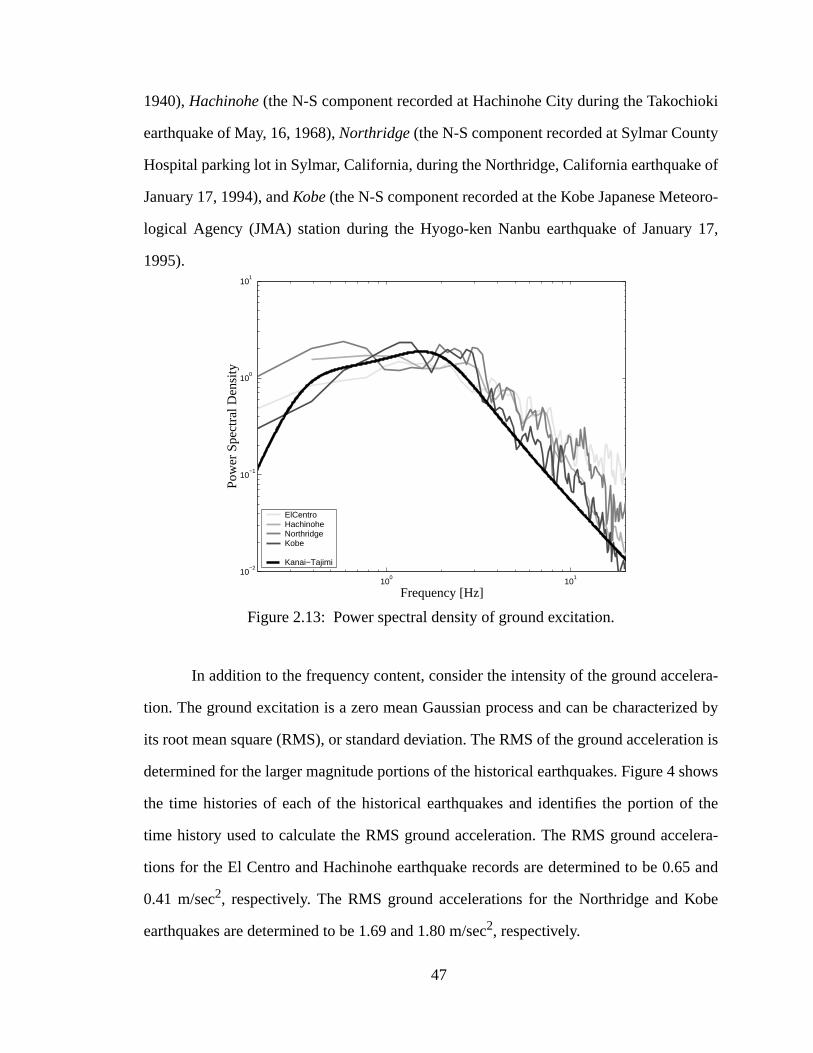
ioki
ty
of
oro-
17,
lera-
ized by
ion is
hows
f the
lera-
5 and
obe
1940),Hachinohe(the N-S component recorded at Hachinohe City during the Takoch
earthquake of May, 16, 1968),Northridge(the N-S component recorded at Sylmar Coun
Hospital parking lot in Sylmar, California, during the Northridge, California earthquake
January 17, 1994), andKobe(the N-S component recorded at the Kobe Japanese Mete
logical Agency (JMA) station during the Hyogo-ken Nanbu earthquake of January
1995).
In addition to the frequency content, consider the intensity of the ground acce
tion. The ground excitation is a zero mean Gaussian process and can be character
its root mean square (RMS), or standard deviation. The RMS of the ground accelerat
determined for the larger magnitude portions of the historical earthquakes. Figure 4 s
the time histories of each of the historical earthquakes and identifies the portion o
time history used to calculate the RMS ground acceleration. The RMS ground acce
tions for the El Centro and Hachinohe earthquake records are determined to be 0.6
0.41 m/sec2, respectively. The RMS ground accelerations for the Northridge and K
earthquakes are determined to be 1.69 and 1.80 m/sec2, respectively.
100
101
10−2
10−1
100
101
Pow
er S
pect
ral D
ensi
ty
Frequency [Hz]
ElCentro Hachinohe Northridge Kobe Kanai−Tajimi
Figure 2.13: Power spectral density of ground excitation.
47
three
r-field
et to
ss of
itation.
ld
From the analysis of RMS ground accelerations of historical earthquakes,
levels of intensity of the ground acceleration are chosen. The first level represents fa
El Centro and Hachinohe type earthquakes and is set to 0.5 m/sec2. The second level rep-
resents near-field Northridge and Kobe type earthquakes and is set to 1.75 m/sec2. The
third level of RMS ground acceleration is considered as an upper bound and is s
3.27 m/sec2.
Measure of Performance
Root mean square (RMS) responses are useful in determining the effectivene
various system parameters on the overall response of the system to a random exc
0 5 10 15 20 25 30 35 40−10
0
10
0 5 10 15 20 25 30 35 40−10
0
10
0 5 10 15 20 25 30 35 40−10
0
10
0 5 10 15 20 25 30 35 40−10
0
10
Figure 2.14: Estimating RMS ground motions from historical records, where the bosection defines the portion of the earthquake used for the RMS calculation.
El C
entr
oH
achi
nohe
Nor
thrid
geK
obe
48
ystem
wn in
the
rmined
, the
e sys-
nsem-
d as the
into
. It is
8), that
link
pling
re
evered
ion is
trum.
The covariance of the state vector and output of the first order linear state space s
defined in Equations (2.16)-(2.17) can be found using the Lyapunov equation (as sho
Appendix A).
An optimal semiactive damping control strategy is applied to this system. For
uncoupled, passive and active cases, RMS values for the linear systems can be dete
analytically via the Lyapunov equation. For the nonlinear semiactive damping case
RMS values must be determined via simulation. As stated earlier, the responses of th
tem are stationary, and, in fact, they are also ergodic. Ergodicity demands that the e
ble average (mean) is equal to the time average. The RMS responses are determine
square root of the mean squares of a discrete series of time values
(2.23)
where is the evaluation output defined in Equation (2.17), , where is the
time step of the simulation, andn is sufficiently large.
2.5 Chapter Summary
In this chapter, a 2DOF coupled building model is examined to provide insight
the effect of passively coupling two structures on the dynamics of the coupled system
observed from the 2DOF model, as has been noted in previous research (Seto, 199
to add damping to the coupled building system, the viscous damping of the coupling
should be increased to some optimal, yet finite, value. Adding stiffness to the cou
link only serves to shift the frequencies of the coupled building system.
Additionally, a MDOF coupled building model is developed. The buildings a
modeled using the Galerkin method, where the mode shapes of the uncoupled cantil
beam are used to represent the behavior of the tall coupled building. A ground excitat
modeled as a filtered white noise process corresponding to the Kanai-Tajimi spec
yerms 1
n--- ye ti( )2
i 1=
n
∑=
ye ti i ∆t( )= ∆t
49

ea-
ter,
ing
and
trol
poses
f cou-
Maximum absolute RMS story acceleration and interstory drift ratio are identified as m
sure of performance for the coupled building system.
A MDOF coupled building model, as developed in the latter part of this chap
can provide further insight into coupled building considerations. The coupled build
configuration, including the relative height, mass, and stiffness of the two buildings,
the height of the coupling link, is important in the design of a coupled building con
strategy, as it can significantly effect the performance of the system. Chapter 3 pro
some new control strategies and examines analytical studies on the performance o
pled building control using the MDOF coupled building model.
50
lem.
ntrol
is-
l
m-
s are
d. A
high-
ree-
gain
sing
d
tes of
CHAPTER 3: COUPLED BUILDING CONTROL: ANALYTICAL STUDIES
This chapter details the analytical studies on the coupled building control prob
Two coupled building control strategies are proposed in this chapter: an active co
strategy employingH2/LQG control with absolute building acceleration and actuator d
placement feedback, and a semiactive control strategy employing clipped optimaH2/
LQG control. The effect of building configuration on coupled building control is exa
ined, where building heights, connector location, building mass, and building stiffnes
varied. The efficacy of semiactive control for the coupled building problem is examine
low-rise coupled building system is also considered to ensure the results shown for
rise structures are similar for their low-rise counterparts.
3.1 Coupled Building Control Strategies
The coupled building control strategies are applied to the high-rise multi-deg
of-freedom (MDOF) coupled building system developed in Section 2.4, and shown a
here in Figure 3.1. The evaluation model for the coupled building system is obtained u
the Galerkin method, where the response of thekth building is assumed to be represente
by the finite series
(3.1)
where is a vector of trial functions for thekth building, as defined in Appendix B as
the mode shapes of a cantilevered beam, and is a vector of generalized coordina
thekth building.
xk y t,( ) fkT
y( )qk t( )=
fk
qk
51
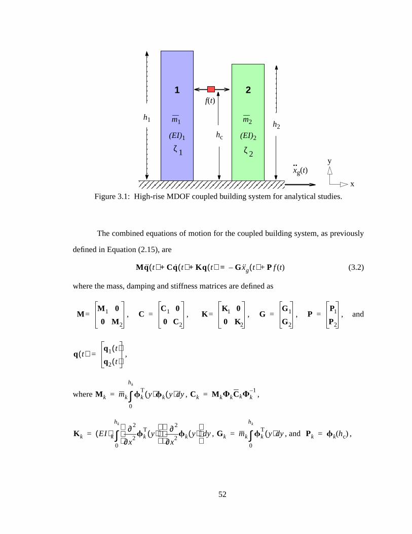
usly
The combined equations of motion for the coupled building system, as previodefined in Equation (2.15), are
(3.2)
where the mass, damping and stiffness matrices are defined as
, , , , , and
,
where , ,
, , and ,
..
1 2
h2h1 m2m1
f(t)
xg(t)
(EI)1 (EI)2
Figure 3.1: High-rise MDOF coupled building system for analytical studies.
ζ 1 ζ 2
x
y
hc
Mq t( ) Cq t( ) Kq t( )+ + G xg t( )– P f t( )+=
MM 1 0
0 M2
= CC1 0
0 C2
= KK1 0
0 K2
= GG1
G2
= PP1
P2
=
q t( )q1 t( )
q2 t( )=
M k mk fkT
y( )fk y( ) yd
0
hk
∫= Ck M kFkCkFk1–
=
K k EI( )kx
2
2
∂∂ fk
Ty( )
x2
2
∂∂ fk y( )
yd
0
hk
∫= Gk mk fkT
y( ) yd
0
hk
∫= Pk fk hc( )=
52
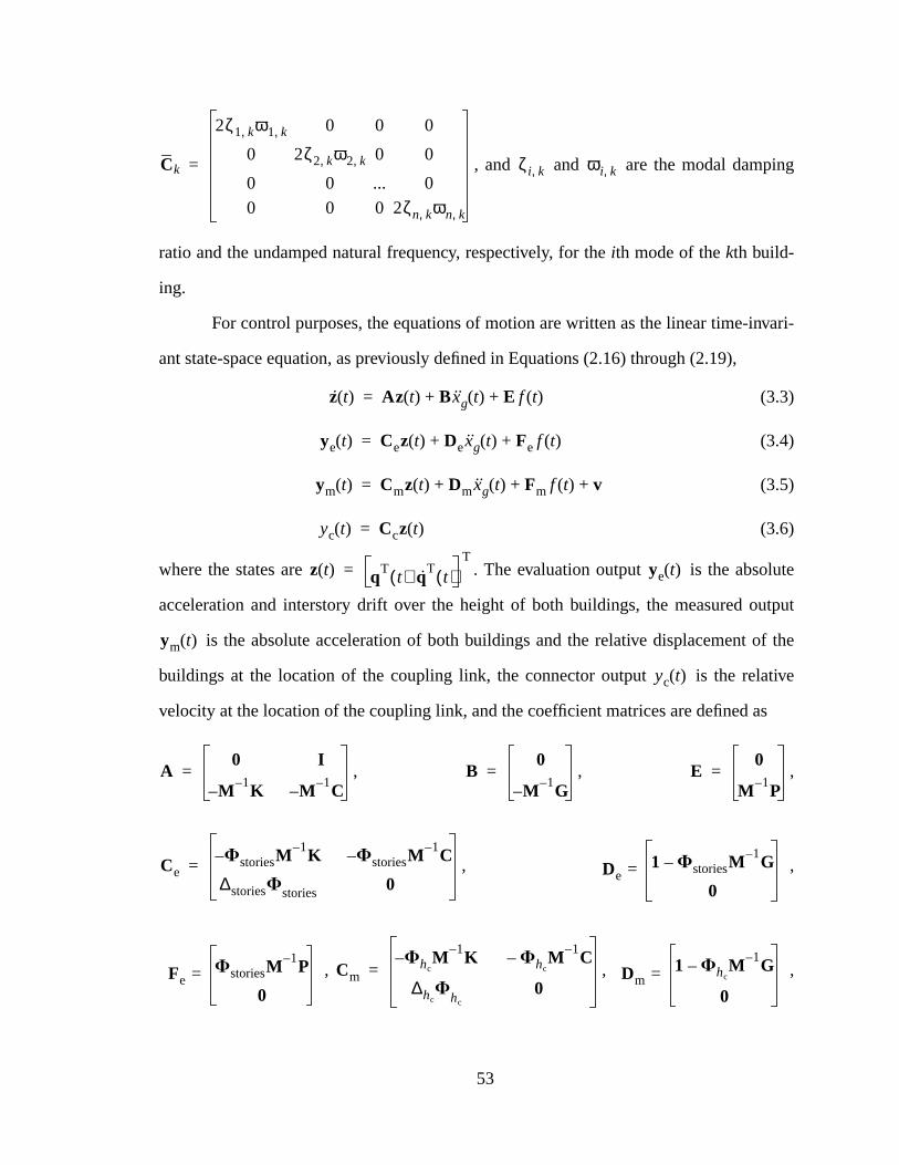
g
vari-
lute
utput
f the
tive
s
, and and are the modal dampin
ratio and the undamped natural frequency, respectively, for theith mode of thekth build-
ing.
For control purposes, the equations of motion are written as the linear time-in
ant state-space equation, as previously defined in Equations (2.16) through (2.19),
(3.3)
(3.4)
(3.5)
(3.6)
where the states are . The evaluation output is the abso
acceleration and interstory drift over the height of both buildings, the measured o
is the absolute acceleration of both buildings and the relative displacement o
buildings at the location of the coupling link, the connector output is the rela
velocity at the location of the coupling link, and the coefficient matrices are defined a
, , ,
, ,
, , ,
Ck
2ζ1 k, ω1 k, 0 0 0
0 2ζ2 k, ω2 k, 0 0
0 0 ... 0
0 0 0 2ζn k, ωn k,
= ζi k, ωi k,
z t( ) Az t( ) B xg t( ) E f t( )+ +=
ye t( ) Cez t( ) Dexg t( ) Fe f t( )+ +=
ym t( ) Cmz t( ) Dmxg t( ) Fm f t( ) v+ + +=
yc t( ) Ccz t( )=
z t( ) qTt( ) qT
t( )T
= ye t( )
ym t( )
yc t( )
A0 I
M–1– K M–
1– C= B
0
M–1– G
= E0
M 1– P=
CeF– storiesM
1– K F– storiesM1– C
∆storiesFstories 0= De
1 F– storiesM1– G
0=
FeFstoriesM
1– P
0= Cm
F– hcM 1– K F– hc
M 1– C
∆hcF
hc0
= Dm1 F– hc
M 1– G
0=
53
f
.
e of
ntrol
iactive
on-
e and
uild-
excita-
eler-
tputs,
, and , where ,
, , , and
, and where is the building story height,
is a vector of the story heights for thekth building withnk stories, and is the height o
the coupling link. Note here the notation
The coupled building control strategies define the second input, , the forc
the coupling link, defined by the passive, active, or semiactive control. The passive co
strategy, as defined in Section 2.4, is to serve as a baseline against which the sem
damping control strategy is compared. Additionally, comparison with the fully active c
trol strategy is useful as it bounds the achievable performance. The proposed activ
semiactive control strategies are identified subsequently.
Active Control Strategy Employing Acceleration Feedback
The active control forces are realized by a control actuator connecting the b
ings at the height , as shown in Figure 3.1.H2/LQG control theory is used. A filter is
augmented to the model of the structural system to shape the spectral content of the
tion in theH2/LQG design. The same Kanai-Tajimi filter used to shape the ground acc
ation for evaluation purposes is used here in the control design. The evaluation ou
, as defined in Equation (3.4) are minimized using the cost function
FmFhc
M 1– P
0= Cc 0 ∆hc
Fhc
= Fstoriesf1
T h1( )
f2T h2( )
=
∆stories∆stories,1 0
0 ∆stories,2
= ∆stories,i
1 0 0
1– 1 0
... 0
0 0 1– 1
= Fhc
f1T
hc( )
f2T
hc( )=
∆hc 1– 1= ∆h hk ∆h 2 ∆h( ) ... nk ∆h( )T
=
hc
fkT hk( ) fk 1∆h( ) fk 2∆h( ) ... fk nk∆h( )
T=
f t( )
hc
ye t( )
54
pro-
(3.3)
ce
ighted
and
tion
xperi-
ncon-
ther
loca-
s of
both
was
f the
MS
oes
(3.7)
where is a weighting matrix for the evaluation outputs. The active control force is
portional to the state estimate
(3.8)
where is an estimate of the state and , where is defined in Equation
and satisfies the algebraic Riccati equation
(3.9)
By varying the weighting matrix , a family of controllers that use varying for
levels can be designed. The absolute accelerations and interstory drift ratios are we
in this study through a matrix of the following form
(3.10)
where is a diagonal matrix to weight the story responses over the two buildings
and are coefficients to weight the relative importance of absolute accelera
and interstory drift responses. It is desired to place larger weight on the stories that e
enced the larger responses. The diagonal elements of the matrix are set to the u
trolled absolute root mean square (RMS) story accelerations of the two buildings. O
forms of considered were: a vector of ones; a vector of zeros with 1 at the story
tion of maximum absolute RMS acceleration; uncontrolled interstory drift response
the two buildings; and vectors of each of the first few uncoupled mode shapes of
buildings. The matrix equal to the uncontrolled absolute RMS story accelerations
found to be most effective in reducing the maximum absolute RMS acceleration o
coupled building system.
The weights and are varied such that the maximum absolute R
accelerations are minimized while ensuring that the maximum interstory drift ratio d
J1τ---E ye
Tt( )Qye t( ) f
2t( )+( ) td
0
τ
∫τ ∞→lim=
Q
f t( ) Kz–=
z K EP= E
P
ATP PA PEETP– Q+ + 0=
Q
Q
QαaccelΨ 0
0 αdriftΨ=
Ψ
αaccel αdrift
Ψ
Ψ
Ψ
αaccel αdrift
55
t the
and
d, as
nal
for
are
s
gni-
ta-
y the
ce of
ave a
con-
e per-
ink,
not get larger than the maximum uncoupled interstory drift ratio. This assumes tha
maximum interstory drift ratio is small enough that the buildings remain undamaged
the critical response is then the acceleration. A maximum drift ratio of 0.005 is use
specified by the Structural Engineers Association of California’s (SEAOC) “operatio
performance” level (Vision 2000 Committee, 1995). This assumption will be examined
the coupled building example presented in Section 3.3. The optimal and
determined from a systematic search over a range of weights.
A standard Kalman filter observer is used to estimate the states of the system
(3.11)
where is the estimator gain and i
computed from the Riccati equation
(3.12)
where is the magnitude of the excitation spectral density , the ma
tude of noise spectral density , , , where is the expec
tion operator, and excitation and sensor noise are uncorrelated. For this stud
measurement noise for the two accelerometers is assumed to have a varian
(m/sec2)2 and the measurement noise for the displacement is assumed to h
variance of m2. The measurement noise corresponds to about 0.1% of the un
trolled RMS responses, respectively. The noise was not seen to significantly affect th
formance of the controller.
The H2/LQG controller, designed using the Control Toolbox in MATLAB , is
employed to determine and . The optimal active control force in the coupling l
, as determined from Equations (3.8) and (3.11), is given by
αaccel αdrift
z A K KFCm–( )z K KFym E K KFFm–( ) f t( )+ +=
K KF PCmT BQKFDm
T+( ) RKF DmQKFDmT
+( ) 1–= P
AP PAT PCmT BQKFDm
T+( ) RKF DmQKFDmT+( ) 1– CmP DmQKFBT+( )–+
BQKFBT–=
QKF Sxgxgω( ) RKF
Svv ω( ) E xg[ ] 0= E v[ ] 0= E ·[ ]
xg v
66–×10
43–×10
K K KF
factv
t( )
56
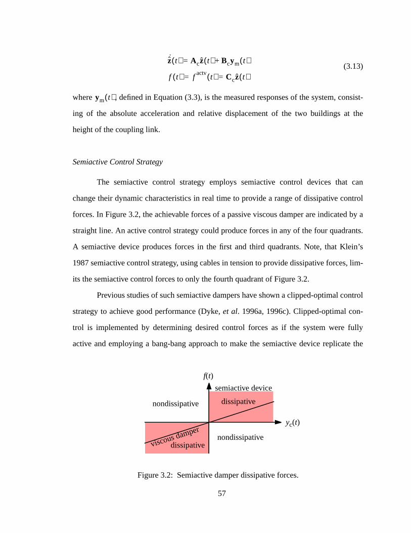
nsist-
t the
can
ntrol
d by a
ants.
ein’s
, lim-
ntrol
-
fully
te the
(3.13)
where , defined in Equation (3.3), is the measured responses of the system, co
ing of the absolute acceleration and relative displacement of the two buildings a
height of the coupling link.
Semiactive Control Strategy
The semiactive control strategy employs semiactive control devices that
change their dynamic characteristics in real time to provide a range of dissipative co
forces. In Figure 3.2, the achievable forces of a passive viscous damper are indicate
straight line. An active control strategy could produce forces in any of the four quadr
A semiactive device produces forces in the first and third quadrants. Note, that Kl
1987 semiactive control strategy, using cables in tension to provide dissipative forces
its the semiactive control forces to only the fourth quadrant of Figure 3.2.
Previous studies of such semiactive dampers have shown a clipped-optimal co
strategy to achieve good performance (Dyke,et al. 1996a, 1996c). Clipped-optimal con
trol is implemented by determining desired control forces as if the system were
active and employing a bang-bang approach to make the semiactive device replica
z t( ) Acz t( ) Bcym t( )+=
f t( ) factv
t( ) Ccz t( )= =
ym t( )
Figure 3.2: Semiactive damper dissipative forces.
f(t)
yc(t)
viscous damper
semiactive device
dissipative
nondissipative
nondissipative
dissipative
57
orces
k,
of
vari-
s of
l are
d the
nd
es of
ion
e floor
iffness
ant to
in the
d the
con-
desired forces. The ideal semiactive device can only produce dissipative control f
given as
(3.14)
where is the relative velocity across the coupling lin
as defined for Equation (3.3).
3.2 Effects of Building Configuration on RMS Response
The building configuration is defined by the height of the buildings, the location
the coupling link, and the mass density and stiffness of the buildings. In this section,
ous configurations are considered, along with their effect on the coupling capabilitie
actively and passively controlled coupled building systems. Active and passive contro
examined as they provide an upper and lower bound to semiactive control, an
responses to these linear systems is more readily available.
The parameters , and are fixed for the taller 50-story building, a
the following ratios are examined for their effects on the response reduction capabiliti
the coupled building system: (i) height ratio ; (ii ) normalized coupling height
; and (iii ) mass density and stiffness ratio . The assumpt
is made that increasing the mass density is accomplished by increasing the size of th
space and is directly related to an increase in the stiffness. Keeping the mass and st
ratios equal has the benefit of leaving the natural frequencies of the system const
study the effect of varying the mass density and stiffness independently of changes
natural frequencies. The examination is done in two parts. First, the height ratio an
coupling link location are varied while holding the mass density and stiffness ratio
f t( )f
actvt( ) f
actvt( ) yc t( ) 0<⋅
0 factv
t( ) yc t( ) 0≥⋅
=
yc t( ) ∆ x hc( ) x2 hc( ) x1 hc( )–= =
h1 m1 EI( )1
h2 h1⁄
hc h2⁄ m2 m1⁄ EI( )2 EI( )1⁄=
58
fness
ith
n-
for
o the
are
first
nam-
6.89,
t of
tical
alu-
tation
he
ild-
se
er-
tory
el
the
stant. Next, the link location is fixed and the height ratio and the mass density and stif
ratio are varied.
The parameters of building 1 are fixed to that of a 50-story high-rise building w
height m. The story height for both buildings is m. The mass de
sity (mass per unit height) of building 1 is kg/m. The stiffness parameter
building 1 is N-m2, where is Young’s Modulus and is the
moment of inertia of the building. is, then, a beam bending stiffness comparable t
composite stiffness of the building.
An in-plane model is developed for the coupled building system. The buildings
each modeled as flexural (Euler-Bernoulli) beams using the Galerkin method. The
five modes of each building are included in the analysis to capture the significant dy
ics of the system. The first five natural frequencies of building 1 are: 0.20, 1.25, 3.51,
and 11.39 Hz. The natural frequencies of building 2 will vary depending on the heigh
the building. Classical viscous damping is assumed for each building, with 1% of cri
damping in each mode.
Consider the transfer function from the ground acceleration to the ev
ation/regulated outputs of a single building model and the Laplace domain represen
of the Kanai-Tajimi filter from Equations (2.21) and (2.22). While observing t
transfer function provides insight into the frequency characteristics of the bu
ing model, the quantity provides insight into the respon
of the building model to the filtered ground excitation. This insight is beneficial in und
standing the behavior of the coupled building system.
The magnitude of for the absolute acceleration of the roof and inters
drift ratio of the top floor are shown in Figure 3.3 for the 50-story building mod
described previously and for 30-story (120 m) and 20-story (80 m) buildings with
same mass density and stiffness parameters.
h1 200= ∆h 4.0=
m1 45×10=
EI( )1 8.1813×10= E I
EI
Hyexgω( )
Hxgwω( )
Hyexgω( )
Hyewω( ) Hyexg
ω( ) Hxgwω( )⋅=
Hyewω( )
59
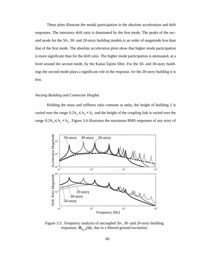
drift
sec-
than
ation
, at a
uild-
g it is
2 is
the
ry of
These plots illustrate the modal participation in the absolute acceleration and
responses. The interstory drift ratio is dominated by the first mode. The peaks of the
ond mode for the 50-, 30- and 20-story building models is an order of magnitude less
that of the first mode. The absolute acceleration plots show that higher mode particip
is more significant than for the drift ratio. The higher mode participation is attenuated
level around the second mode, by the Kanai-Tajimi filter. For the 50- and 30-story b
ings the second mode plays a significant role in the response, for the 20-story buildin
less.
Varying Building and Connector Heights
Holding the mass and stiffness ratio constant at unity, the height of building
varied over the range and the height of the coupling link is varied over
range . Figure 3.4 illustrates the maximum RMS responses of any sto
10−1
100
101
102
10−2
100
102
Acc
eler
atio
n M
agni
tude
Frequency [Hz]
10−1
100
101
102
10−5
100
Drif
t Ang
le M
agni
tude
102
n M
agni
tude
Frequency [Hz]
Figure 3.3: Frequency analysis of uncoupled 50-, 30- and 20-story buildingresponses, , due to a filtered ground excitation.Hyew
ω( )
50-story 30-story 20-story
50-story30-story
20-story
Rat
io
0.2h1 h2 h1<≤
0.2h2 hc h2<≤
60
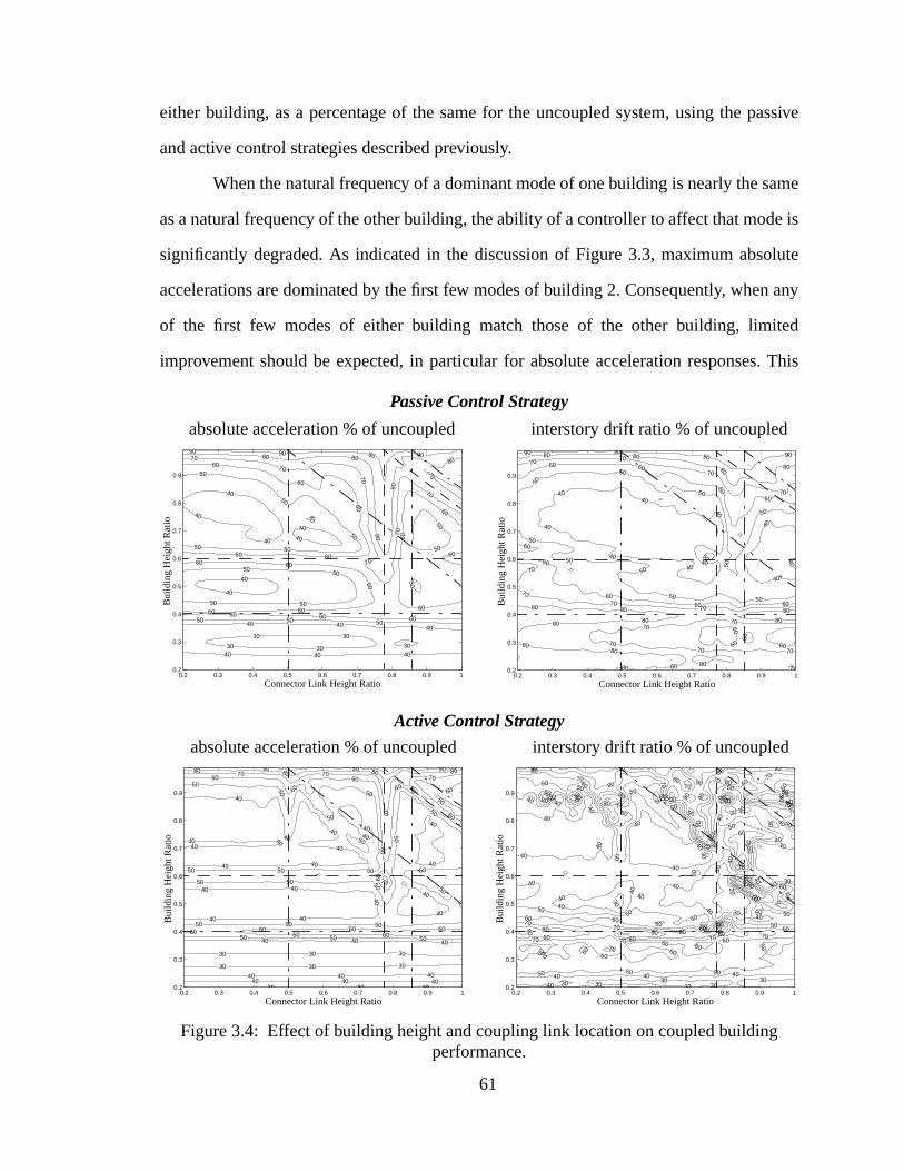
assive
ame
e is
olute
n any
ted
. This
ed
ed
either building, as a percentage of the same for the uncoupled system, using the p
and active control strategies described previously.
When the natural frequency of a dominant mode of one building is nearly the s
as a natural frequency of the other building, the ability of a controller to affect that mod
significantly degraded. As indicated in the discussion of Figure 3.3, maximum abs
accelerations are dominated by the first few modes of building 2. Consequently, whe
of the first few modes of either building match those of the other building, limi
improvement should be expected, in particular for absolute acceleration responses
0.2 0.3 0.4 0.5 0.6 0.7 0.8 0.9 10.2
0.3
0.4
0.5
0.6
0.7
0.8
0.9
Connector Link Height Ratio
Bui
ldin
g H
eigh
t Rat
io
20
303030
3030
30
30
30
30
30
30
30
30
30
30
30
40
40
40
40
40
40
40 40 40
4040
40
40
40
40
40
40
40
4040
40
40
40
40
40
40
40
50
50
50
50
50
50
50
50
5050
5050
50 50 50
50
50
50
50
50
50
50
50
50
50
50
60 60
60
60
60
60
60
60 6060 60
6060 6060
60 60
60
60
60
60
60
60
60
60
60
70
70
70
70
70 70
7070 70
707070
70
70
70
70
70
70
70
70
70
70
70
80
80
80
80
80
8080
8080
80
80
80
80
80
8080
80
80
80
90 90
90
90
90
90
90
90
90
90
9090
90
90
90
100
0.2 0.3 0.4 0.5 0.6 0.7 0.8 0.9 10.2
0.3
0.4
0.5
0.6
0.7
0.8
0.9
Connector Link Height Ratio
Bui
ldin
g H
eigh
t Rat
io
40
40
40
40
40
4040
40
4040
50
50
50
50
50
50
50
50
50 50
50
60 60
60
60
60
60
6060 60
60
60
60
60
7070
70
70
70
70
7070
7070
7070 70
7080 80
8080
80 80
80
80
80 80
8080
80
80
80
90 9090 90
0.2 0.3 0.4 0.5 0.6 0.7 0.8 0.9 10.2
0.3
0.4
0.5
0.6
0.7
0.8
0.9
Connector Link Height Ratio
Bui
ldin
g H
eigh
t Rat
io
30 30
3030
30
40
40
40
40 40 40
40 40 40
40
40
40
40
40
50
50
505050
50 50
5050
50 50 50
50
50
50
60
60
60
606060 60
60
6060 60 60 60
60
60
60
60
70
70
70
70
70
70
70
80 80
80
80
8090909090
0.2 0.3 0.4 0.5 0.6 0.7 0.8 0.9 10.2
0.3
0.4
0.5
0.6
0.7
0.8
0.9
Connector Link Height Ratio
Bui
ldin
g H
eigh
t Rat
io
30 30 30
30 30 30
30 30 30
40
4040
40
4040
40 40
40
40 40
40
4040
40 40 40
40 40 4040 40 40
40
40
40
40
4040
50
50
50
50
505050
50 50 50
50
50
50 50 50
50 50 50
50
50
50
50
60
60
60
60
60
60
60
60 60606060 60
60
70 70
70
70
70
70
80808080 909090
Figure 3.4: Effect of building height and coupling link location on coupled buildingperformance.
absolute acceleration % of uncoupled interstory drift ratio % of uncoupl
Passive Control Strategy
Active Control Strategy
absolute acceleration % of uncoupled interstory drift ratio % of uncoupl
61
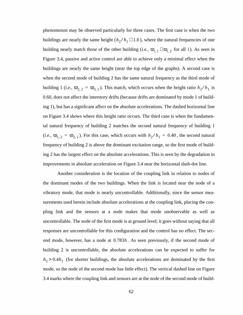
e two
f one
n the
ase is
de of
is
uild-
al line
men-
ng 1
ral
uild-
tion in
e.
of
of a
ea-
e cou-
ll as
at all
e sec-
de of
r for
first
igure
build-
phenomenon may be observed particularly for three cases. The first case is when th
buildings are nearly the same height ( ), where the natural frequencies o
building nearly match those of the other building (i.e., for all ). As seen in
Figure 3.4, passive and active control are able to achieve only a minimal effect whe
buildings are nearly the same height (near the top edge of the graphs). A second c
when the second mode of building 2 has the same natural frequency as the third mo
building 1 (i.e., ). This match, which occurs when the height ratio
0.60, does not affect the interstory drifts (because drifts are dominated by mode 1 of b
ing 1), but has a significant affect on the absolute accelerations. The dashed horizont
on Figure 3.4 shows where this height ratio occurs. The third case is when the funda
tal natural frequency of building 2 matches the second natural frequency of buildi
(i.e., ). For this case, which occurs with , the second natu
frequency of building 2 is above the dominant excitation range, so the first mode of b
ing 2 has the largest effect on the absolute accelerations. This is seen by the degrada
improvements in absolute acceleration on Figure 3.4 near the horizontal dash-dot lin
Another consideration is the location of the coupling link in relation to nodes
the dominant modes of the two buildings. When the link is located near the node
vibratory mode, that mode is nearly uncontrollable. Additionally, since the sensor m
surements used herein include absolute accelerations at the coupling link, placing th
pling link and the sensors at a node makes that mode unobservable as we
uncontrollable. The node of the first mode is at ground level; it goes without saying th
responses are uncontrollable for this configuration and the control has no effect. Th
ond mode, however, has a node at . As seen previously, if the second mo
building 2 is uncontrollable, the absolute accelerations can be expected to suffe
(for shorter buildings, the absolute accelerations are dominated by the
mode, so the node of the second mode has little effect). The vertical dashed line on F
3.4 marks where the coupling link and sensors are at the node of the second mode of
h2 h1⁄ 1.0≅
ωi 1, ωi 2,≅ i
ω2 2, ω3 1,= h2 h1⁄
ω1 2, ω2 1,= h2 h1⁄ 0.40=
0.783h
h2 0.4h1>
62
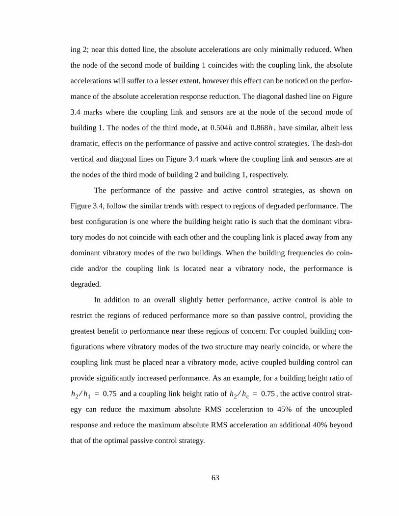
hen
lute
erfor-
Figure
de of
ess
sh-dot
re at
n on
. The
ibra-
any
oin-
e is
to
g the
con-
e the
can
io of
t-
pled
eyond
ing 2; near this dotted line, the absolute accelerations are only minimally reduced. W
the node of the second mode of building 1 coincides with the coupling link, the abso
accelerations will suffer to a lesser extent, however this effect can be noticed on the p
mance of the absolute acceleration response reduction. The diagonal dashed line on
3.4 marks where the coupling link and sensors are at the node of the second mo
building 1. The nodes of the third mode, at and , have similar, albeit l
dramatic, effects on the performance of passive and active control strategies. The da
vertical and diagonal lines on Figure 3.4 mark where the coupling link and sensors a
the nodes of the third mode of building 2 and building 1, respectively.
The performance of the passive and active control strategies, as show
Figure 3.4, follow the similar trends with respect to regions of degraded performance
best configuration is one where the building height ratio is such that the dominant v
tory modes do not coincide with each other and the coupling link is placed away from
dominant vibratory modes of the two buildings. When the building frequencies do c
cide and/or the coupling link is located near a vibratory node, the performanc
degraded.
In addition to an overall slightly better performance, active control is able
restrict the regions of reduced performance more so than passive control, providin
greatest benefit to performance near these regions of concern. For coupled building
figurations where vibratory modes of the two structure may nearly coincide, or wher
coupling link must be placed near a vibratory mode, active coupled building control
provide significantly increased performance. As an example, for a building height rat
and a coupling link height ratio of , the active control stra
egy can reduce the maximum absolute RMS acceleration to 45% of the uncou
response and reduce the maximum absolute RMS acceleration an additional 40% b
that of the optimal passive control strategy.
0.504h 0.868h
h2 h1⁄ 0.75= h2 hc⁄ 0.75=
63
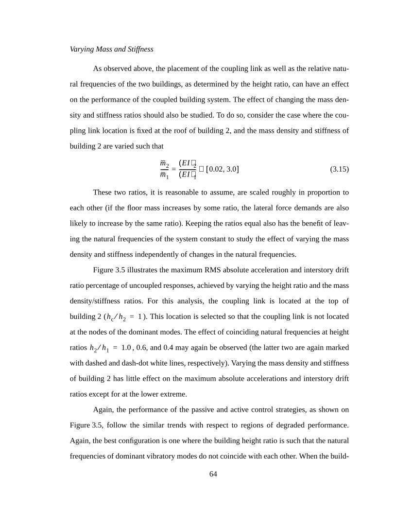
atu-
effect
den-
e cou-
s of
on to
e also
leav-
mass
drift
e mass
of
ted
eight
rked
ffness
drift
n on
nce.
tural
uild-
Varying Mass and Stiffness
As observed above, the placement of the coupling link as well as the relative n
ral frequencies of the two buildings, as determined by the height ratio, can have an
on the performance of the coupled building system. The effect of changing the mass
sity and stiffness ratios should also be studied. To do so, consider the case where th
pling link location is fixed at the roof of building 2, and the mass density and stiffnes
building 2 are varied such that
(3.15)
These two ratios, it is reasonable to assume, are scaled roughly in proporti
each other (if the floor mass increases by some ratio, the lateral force demands ar
likely to increase by the same ratio). Keeping the ratios equal also has the benefit of
ing the natural frequencies of the system constant to study the effect of varying the
density and stiffness independently of changes in the natural frequencies.
Figure 3.5 illustrates the maximum RMS absolute acceleration and interstory
ratio percentage of uncoupled responses, achieved by varying the height ratio and th
density/stiffness ratios. For this analysis, the coupling link is located at the top
building 2 ( ). This location is selected so that the coupling link is not loca
at the nodes of the dominant modes. The effect of coinciding natural frequencies at h
ratios , 0.6, and 0.4 may again be observed (the latter two are again ma
with dashed and dash-dot white lines, respectively). Varying the mass density and sti
of building 2 has little effect on the maximum absolute accelerations and interstory
ratios except for at the lower extreme.
Again, the performance of the passive and active control strategies, as show
Figure 3.5, follow the similar trends with respect to regions of degraded performa
Again, the best configuration is one where the building height ratio is such that the na
frequencies of dominant vibratory modes do not coincide with each other. When the b
m2
m1------
EI( )2
EI( )1-------------= 0.02 3.0,[ ]∈
hc h2⁄ 1=
h2 h1⁄ 1.0=
64
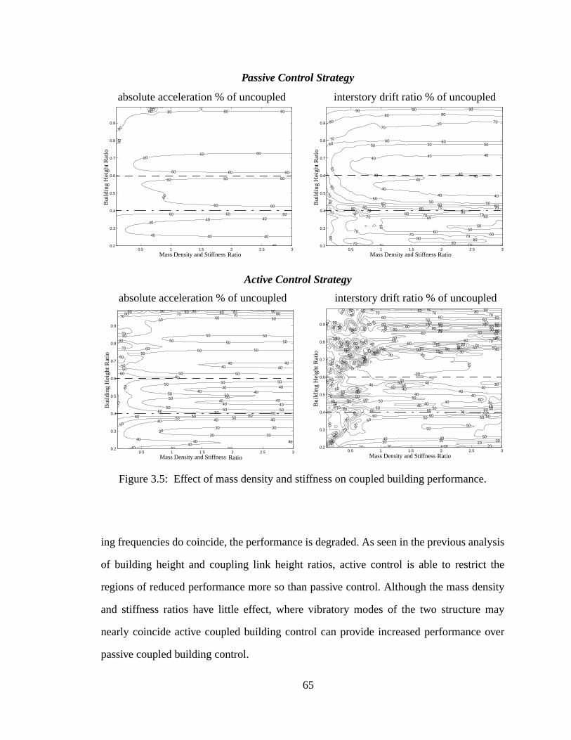
alysis
the
ensity
may
over
e.
d
ed
ing frequencies do coincide, the performance is degraded. As seen in the previous an
of building height and coupling link height ratios, active control is able to restrict
regions of reduced performance more so than passive control. Although the mass d
and stiffness ratios have little effect, where vibratory modes of the two structure
nearly coincide active coupled building control can provide increased performance
passive coupled building control.
0.5 1 1.5 2 2.5 30.2
0.3
0.4
0.5
0.6
0.7
0.8
0.9
Connector Link Height Ratio
Bui
ldin
g H
eigh
t Rat
io
40
404040
40 40 40
60
60 60 60
606060
60 60 60
606060
60
60 60
80
80
80 80 80
80
0.5 1 1.5 2 2.5 30.2
0.3
0.4
0.5
0.6
0.7
0.8
0.9
Connector Link Height Ratio
Bui
ldin
g H
eigh
t Rat
io
30 30
303030
30 30
4040
4040
40 40 40
404040 40
404040 40
404040 40
40
50
5050 50
5050 50
50
50 50
505050 50 50
505050
50 505050
50 50 50
60
60 60 60
60
60
60
6060
60
60 60 6060 60 60
7070 70
70
70
70
80 80 80 8090 90 90 90 90
0.5 1 1.5 2 2.5 30.2
0.3
0.4
0.5
0.6
0.7
0.8
0.9
Connector Link Height Ratio
Bui
ldin
g H
eigh
t Rat
io
404040
4040
40
40 40
4040
505050
50
5050 50
5050
6060 60
60
60 60 60
6060
60
6060
60
70
70
7070 70
70
70 70 70
70707070
7070 70
7080
80
80 80
80
80 808080
80
8080 80
90 90 90
90
0.5 1 1.5 2 2.5 30.2
0.3
0.4
0.5
0.6
0.7
0.8
0.9
Connector Link Height Ratio
Bui
ldin
g H
eigh
t Rat
io
2020
20
20
30 30 30
30 30
30
30
30
30
30
30
30
3030
30
30
4040 40
40
40
4040
40
40
40 4040
4040
40 40
4040
40
4040
40 40
40
4040
50
50 50 50
505050 50 50
5050
5050
50
50
50
50
5050 50
50
50 50 50
50
50
50
50
50
5050
50
5050
60
60 60 60
60
606060
60 60 60
606060
60
60
60
60 60 60
6060
606060
60
60
60
60
60
60
60
70
7070
70
70
70
70
70 70 70
707070 70 70
707070
70
70 70
70
7070
70
70
70
80
80
8080
80 80 80
80
80
80
80
808080
80 80
80
80
80 8080
80
80
80
80
9090
90 90 90
9090
9090
90
90
90
90
90
90
90
9090
909090
100
100
100
100
Figure 3.5: Effect of mass density and stiffness on coupled building performanc
Passive Control Strategy
Active Control Strategy
Mass Density and Stiffness
Mass Density and Stiffness Mass Density and Stiffness
Mass Density and Stiffness
absolute acceleration % of uncoupled interstory drift ratio % of uncouple
absolute acceleration % of uncoupled interstory drift ratio % of uncoupl
65
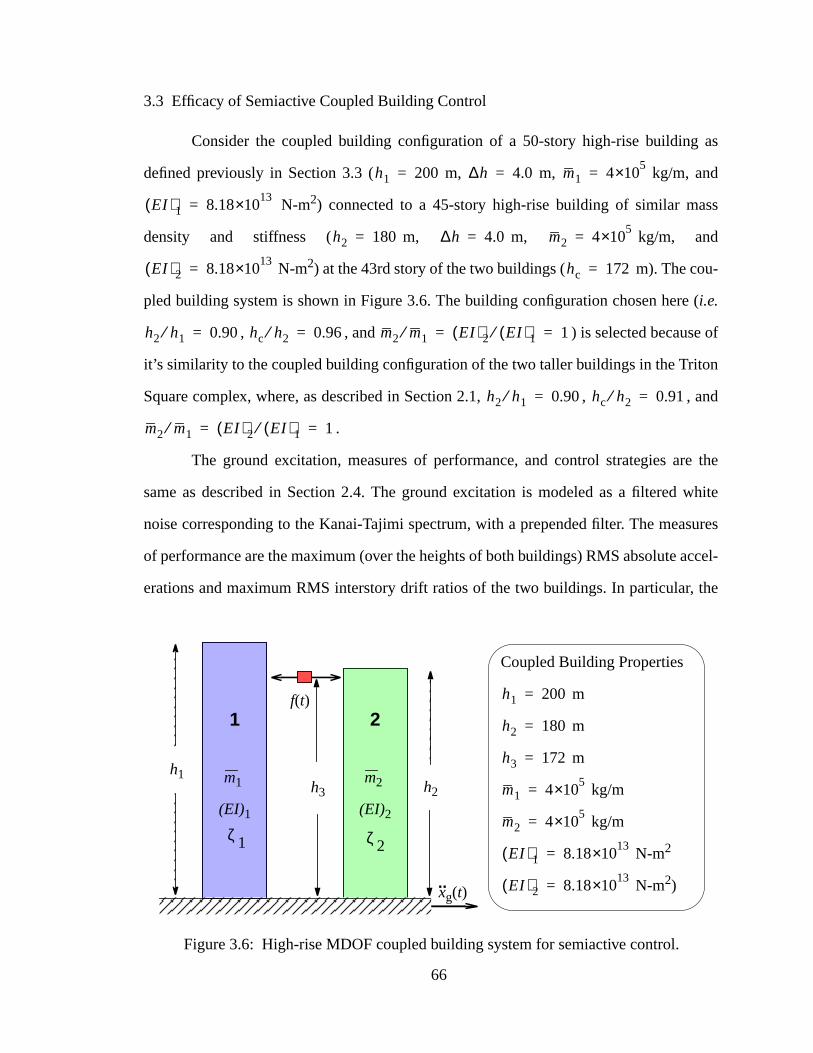
as
d
ss
d
-
(
f
n
and
e the
white
sures
ccel-
the
3.3 Efficacy of Semiactive Coupled Building Control
Consider the coupled building configuration of a 50-story high-rise building
defined previously in Section 3.3 ( m, m, kg/m, an
N-m2) connected to a 45-story high-rise building of similar ma
density and stiffness ( m, m, kg/m, an
N-m2) at the 43rd story of the two buildings ( m). The cou
pled building system is shown in Figure 3.6. The building configuration chosen herei.e.
, , and ) is selected because o
it’s similarity to the coupled building configuration of the two taller buildings in the Trito
Square complex, where, as described in Section 2.1, , ,
.
The ground excitation, measures of performance, and control strategies ar
same as described in Section 2.4. The ground excitation is modeled as a filtered
noise corresponding to the Kanai-Tajimi spectrum, with a prepended filter. The mea
of performance are the maximum (over the heights of both buildings) RMS absolute a
erations and maximum RMS interstory drift ratios of the two buildings. In particular,
h1 200= ∆h 4.0= m1 45×10=
EI( )1 8.1813×10=
h2 180= ∆h 4.0= m2 45×10=
EI( )2 8.1813×10= hc 172=
Figure 3.6: High-rise MDOF coupled building system for semiactive control.
..
1 2
h2
h1 m2m1
f(t)
xg(t)
(EI)1 (EI)2
ζ 1 ζ 2
h3
Coupled Building Properties
m
m
m
kg/m
kg/m
N-m2
N-m2)
h1 200=
h2 180=
h3 172=
m1 45×10=
m2 45×10=
EI( )1 8.1813×10=
EI( )2 8.1813×10=
h2 h1⁄ 0.90= hc h2⁄ 0.96= m2 m1⁄ EI( )2 EI( )1⁄ 1= =
h2 h1⁄ 0.90= hc h2⁄ 0.91=
m2 m1⁄ EI( )2 EI( )1⁄ 1= =
66
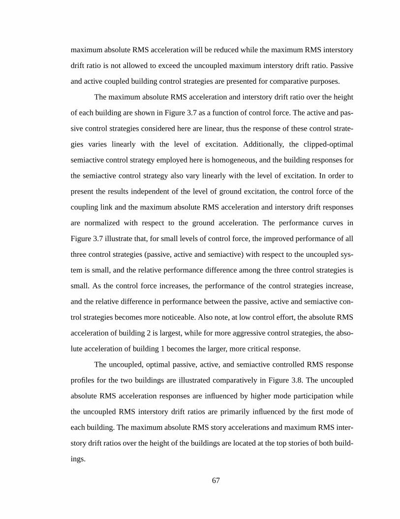
tory
sive
es.
ight
pas-
strate-
al
ses for
r to
f the
nses
es in
f all
d sys-
ies is
rease,
e con-
RMS
abso-
onse
led
while
of
inter-
uild-
maximum absolute RMS acceleration will be reduced while the maximum RMS inters
drift ratio is not allowed to exceed the uncoupled maximum interstory drift ratio. Pas
and active coupled building control strategies are presented for comparative purpos
The maximum absolute RMS acceleration and interstory drift ratio over the he
of each building are shown in Figure 3.7 as a function of control force. The active and
sive control strategies considered here are linear, thus the response of these control
gies varies linearly with the level of excitation. Additionally, the clipped-optim
semiactive control strategy employed here is homogeneous, and the building respon
the semiactive control strategy also vary linearly with the level of excitation. In orde
present the results independent of the level of ground excitation, the control force o
coupling link and the maximum absolute RMS acceleration and interstory drift respo
are normalized with respect to the ground acceleration. The performance curv
Figure 3.7 illustrate that, for small levels of control force, the improved performance o
three control strategies (passive, active and semiactive) with respect to the uncouple
tem is small, and the relative performance difference among the three control strateg
small. As the control force increases, the performance of the control strategies inc
and the relative difference in performance between the passive, active and semiactiv
trol strategies becomes more noticeable. Also note, at low control effort, the absolute
acceleration of building 2 is largest, while for more aggressive control strategies, the
lute acceleration of building 1 becomes the larger, more critical response.
The uncoupled, optimal passive, active, and semiactive controlled RMS resp
profiles for the two buildings are illustrated comparatively in Figure 3.8. The uncoup
absolute RMS acceleration responses are influenced by higher mode participation
the uncoupled RMS interstory drift ratios are primarily influenced by the first mode
each building. The maximum absolute RMS story accelerations and maximum RMS
story drift ratios over the height of the buildings are located at the top stories of both b
ings.
67
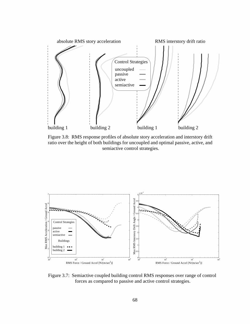
rol
t
105
106
107
108
0
1
2
3
4
5
6
7
Max
RM
S A
ccel
erat
ion
/ Gro
und
Acc
el
RMS Force / Ground Accel [N/(m/sec2)]10
510
610
710
80
0.5
1
1.5
2
2.5
3
3.5
4
4.5
5x 10
−3
Max
RM
S In
ters
tory
Drif
t Ang
le /
Gro
und
Acc
el
RMS Force / Ground Accel [N/(m/sec2)]
Figure 3.7: Semiactive coupled building control RMS responses over range of contforces as compared to passive and active control strategies.
Control Strategies
passiveactivesemiactive
Buildings
building 1building 2
Figure 3.8: RMS response profiles of absolute story acceleration and interstory drifratio over the height of both buildings for uncoupled and optimal passive, active, and
semiactive control strategies.
Control Strategies
passiveactivesemiactive
uncoupled
building 1 building 2 building 1 building 2
absolute RMS story acceleration RMS interstory drift ratio
68
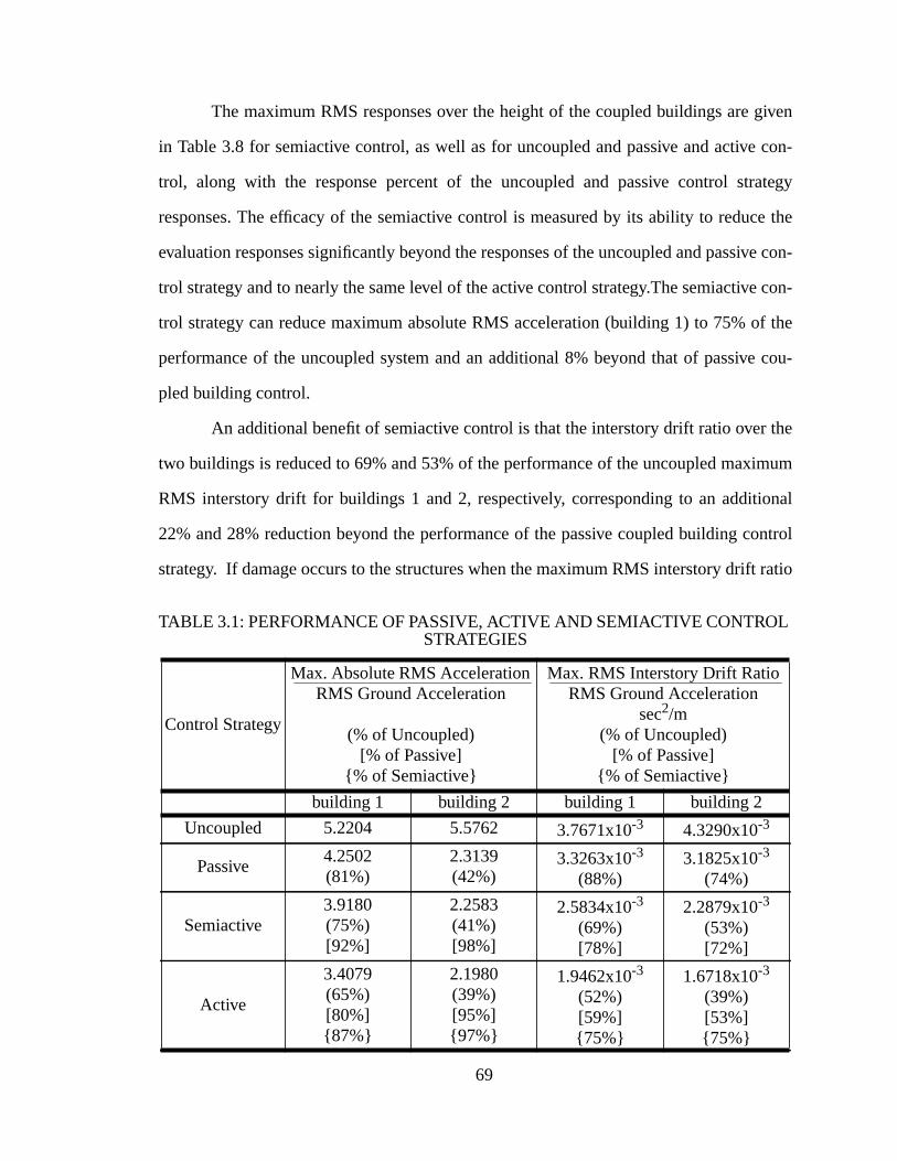
iven
con-
ategy
e the
ve con-
con-
f the
cou-
the
mum
nal
ntrol
ratio
The maximum RMS responses over the height of the coupled buildings are g
in Table 3.8 for semiactive control, as well as for uncoupled and passive and active
trol, along with the response percent of the uncoupled and passive control str
responses. The efficacy of the semiactive control is measured by its ability to reduc
evaluation responses significantly beyond the responses of the uncoupled and passi
trol strategy and to nearly the same level of the active control strategy.The semiactive
trol strategy can reduce maximum absolute RMS acceleration (building 1) to 75% o
performance of the uncoupled system and an additional 8% beyond that of passive
pled building control.
An additional benefit of semiactive control is that the interstory drift ratio over
two buildings is reduced to 69% and 53% of the performance of the uncoupled maxi
RMS interstory drift for buildings 1 and 2, respectively, corresponding to an additio
22% and 28% reduction beyond the performance of the passive coupled building co
strategy. If damage occurs to the structures when the maximum RMS interstory drift
TABLE 3.1: PERFORMANCE OF PASSIVE, ACTIVE AND SEMIACTIVE CONTROLSTRATEGIES
Control Strategy
Max. Absolute RMS AccelerationRMS Ground Acceleration
(% of Uncoupled)[% of Passive]
{% of Semiactive}
Max. RMS Interstory Drift RatioRMS Ground Acceleration
sec2/m(% of Uncoupled)
[% of Passive]{% of Semiactive}
building 1 building 2 building 1 building 2
Uncoupled 5.2204 5.5762 3.7671x10⁻³ 4.3290x10⁻³
Passive4.2502(81%)
2.3139(42%)
3.3263x10⁻³
(88%)3.1825x10⁻³
(74%)
Semiactive3.9180(75%)[92%]
2.2583(41%)[98%]
2.5834x10⁻³
(69%)[78%]
2.2879x10⁻³
(53%)[72%]
Active
3.4079(65%)[80%]{87%}
2.1980(39%)[95%]{97%}
1.9462x10⁻³
(52%)[59%]{75%}
1.6718x10⁻³
(39%)[53%]{75%}
69
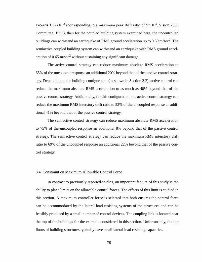
rolled
ccel-
n to
l strat-
l can
of the
can
addi-
ation
ontrol
drift
con-
the
in
force
can be
near
top
exceeds 1.67x10⁻³ (corresponding to a maximum peak drift ratio of 5x10⁻³, Vision 2000
Committee, 1995), then for the coupled building system examined here, the uncont
buildings can withstand an earthquake of RMS ground acceleration up to 0.39 m/sec2. The
semiactive coupled building system can withstand an earthquake with RMS ground a
eration of 0.65 m/sec2 without sustaining any significant damage .
The active control strategy can reduce maximum absolute RMS acceleratio
65% of the uncoupled response an additional 20% beyond that of the passive contro
egy. Depending on the building configuration (as shown in Section 3.2), active contro
reduce the maximum absolute RMS acceleration to as much as 40% beyond that
passive control strategy. Additionally, for this configuration, the active control strategy
reduce the maximum RMS interstory drift ratio to 52% of the uncoupled response an
tional 41% beyond that of the passive control strategy.
The semiactive control strategy can reduce maximum absolute RMS acceler
to 75% of the uncoupled response an additional 8% beyond that of the passive c
strategy. The semiactive control strategy can reduce the maximum RMS interstory
ratio to 69% of the uncoupled response an additional 22% beyond that of the passive
trol strategy.
3.4 Constraint on Maximum Allowable Control Force
In contrast to previously reported studies, an important feature of this study is
ability to place limits on the allowable control forces. The effects of this limit is studied
this section. A maximum controller force is selected that both ensures the control
can be accommodated by the lateral load resisting systems of the structures and
feasibly produced by a small number of control devices. The coupling link is located
the top of the buildings for the example considered in this section. Unfortunately, the
floors of building structures typically have small lateral load resisting capacities.
70
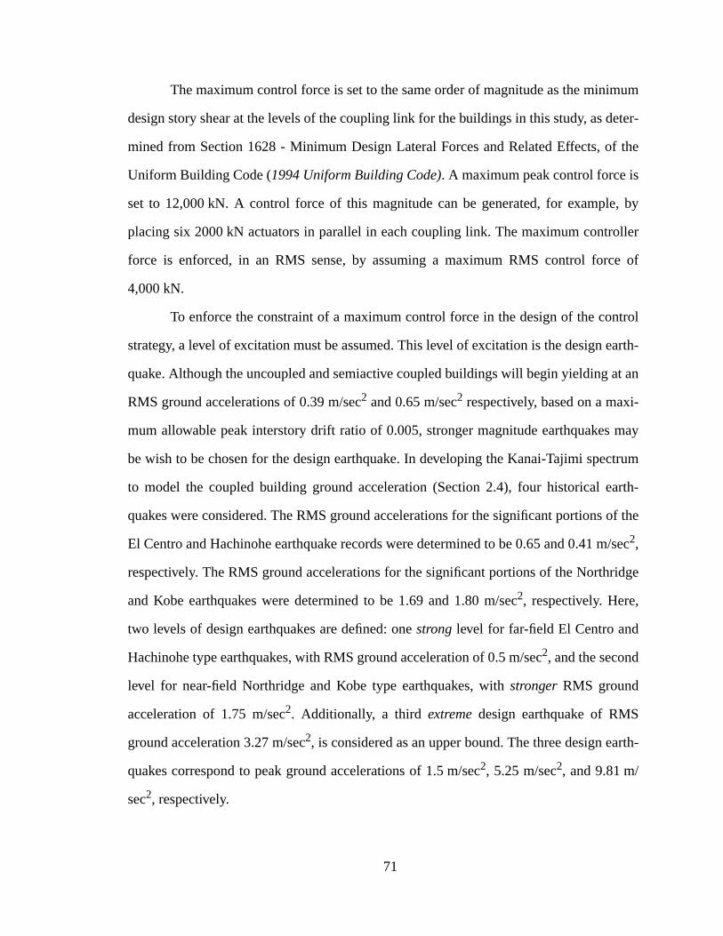
um
eter-
f the
, by
ller
e of
trol
arth-
t an
-
may
ctrum
rth-
of the
/sec
idge
rth-
The maximum control force is set to the same order of magnitude as the minim
design story shear at the levels of the coupling link for the buildings in this study, as d
mined from Section 1628 - Minimum Design Lateral Forces and Related Effects, o
Uniform Building Code (1994 Uniform Building Code). A maximum peak control force is
set to 12,000 kN. A control force of this magnitude can be generated, for example
placing six 2000 kN actuators in parallel in each coupling link. The maximum contro
force is enforced, in an RMS sense, by assuming a maximum RMS control forc
4,000 kN.
To enforce the constraint of a maximum control force in the design of the con
strategy, a level of excitation must be assumed. This level of excitation is the design e
quake. Although the uncoupled and semiactive coupled buildings will begin yielding a
RMS ground accelerations of 0.39 m/sec2 and 0.65 m/sec2 respectively, based on a maxi
mum allowable peak interstory drift ratio of 0.005, stronger magnitude earthquakes
be wish to be chosen for the design earthquake. In developing the Kanai-Tajimi spe
to model the coupled building ground acceleration (Section 2.4), four historical ea
quakes were considered. The RMS ground accelerations for the significant portions
El Centro and Hachinohe earthquake records were determined to be 0.65 and 0.41 m2,
respectively. The RMS ground accelerations for the significant portions of the Northr
and Kobe earthquakes were determined to be 1.69 and 1.80 m/sec2, respectively. Here,
two levels of design earthquakes are defined: onestrong level for far-field El Centro and
Hachinohe type earthquakes, with RMS ground acceleration of 0.5 m/sec2, and the second
level for near-field Northridge and Kobe type earthquakes, withstrongerRMS ground
acceleration of 1.75 m/sec2. Additionally, a third extremedesign earthquake of RMS
ground acceleration 3.27 m/sec2, is considered as an upper bound. The three design ea
quakes correspond to peak ground accelerations of 1.5 m/sec2, 5.25 m/sec2, and 9.81 m/
sec2, respectively.
71
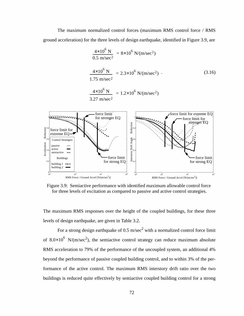
S
9, are
three
lute
l 4%
per-
wo
ong
es.
The maximum normalized control forces (maximum RMS control force / RM
ground acceleration) for the three levels of design earthquake, identified in Figure 3.
. (3.16)
The maximum RMS responses over the height of the coupled buildings, for these
levels of design earthquake, are given in Table 3.2.
For a strong design earthquake of 0.5 m/sec2 with a normalized control force limit
of N/(m/sec2), the semiactive control strategy can reduce maximum abso
RMS acceleration to 79% of the performance of the uncoupled system, an additiona
beyond the performance of passive coupled building control, and to within 3% of the
formance of the active control. The maximum RMS interstory drift ratio over the t
buildings is reduced quite effectively by semiactive coupled building control for a str
46×10 N
0.5 m/sec2------------------------- 8
6×10 N/(m/sec2)=
46×10 N
1.75 m/sec2---------------------------- 2.3
6×10 N/(m/sec2)=
46×10 N
3.27 m/sec2---------------------------- 1.2
6×10 N/(m/sec2)=
105
106
107
108
0
0.2
0.4
0.6
0.8
1
Acc
eler
atio
n %
Red
uctio
n
RMS Force / Ground Accel [N/(m/sec2)]10
510
610
710
80
0.2
0.4
0.6
0.8
1
Inte
rsto
ry D
rift A
ngle
% R
educ
tion
RMS Force / Ground Accel [N/(m/sec2)]
Figure 3.9: Semiactive performance with identified maximum allowable control forcfor three levels of excitation as compared to passive and active control strategie
Control Strategies
passiveactivesemiactive
Buildings
building 1building 2
force limit
force limit
force limit for
force limit
force limit for
for strong EQ
for stronger EQ
extreme EQ
for strong EQ
force limit for extreme EQ
stronger EQ
8.06×10
72
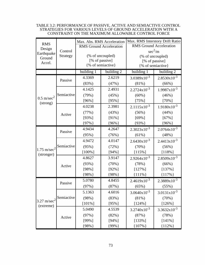
TABLE 3.2: PERFORMANCE OF PASSIVE, ACTIVE AND SEMIACTIVE CONTROLSTRATEGIES FOR VARIOUS LEVELS OF GROUND ACCELERATION WITH A
CONSTRAINT ON THE MAXIMUM ALLOWABLE CONTROL FORCE
RMSDesign
EarthquakeGroundAccel.
ControlStrategy
Max. Abs. RMS AccelerationRMS Ground Acceleration
(% of uncoupled)[% of passive]
{% of semiactive}
Max. RMS Interstory Drift RatioRMS Ground Acceleration
sec2/m(% of uncoupled)
[% of passive]{% of semiactive}
building 1 building 2 building 1 building 2
0.5 m/sec2
(strong)
Passive4.3369 2.6219 3.0389x10⁻³ 2.8530x10⁻³
(83%) (47%) (81%) (66%)
Semiactive4.1425 2.4931 2.2724x10⁻³ 1.9987x10⁻³
(79%) (45%) (60%) (46%)[96%] [95%] [75%] [70%]
Active
4.0238 2.3981 2.1115x10⁻³ 1.9180x10⁻³
(77%) (43%) (56%) (44%)[93%] [91%] [69%] [67%]{97%} {96%} {93%} {96%}
1.75 m/sec2
(stronger)
Passive4.9434 4.2647 2.3023x10⁻³ 2.0764x10⁻³
(95%) (76%) (61%) (48%)
Semiactive4.9472 4.0147 2.6430x10⁻³ 2.4413x10⁻³
(95%) (72%) (70%) (56%)[100%] [94%] [115%] [118%]
Active
4.8627 3.9147 2.9264x10⁻³ 2.8509x10⁻³
(93%) (70%) (78%) (66%)[98%] [92%] [127%] [137%]{98%} {98%} {111%} {117%}
3.27 m/sec2
(extreme)
Passive5.0780 4.8455 2.4619x10⁻³ 2.3889x10⁻³
(97%) (87%) (65%) (55%)
Semiactive5.1363 4.6016 3.0640x10⁻³ 3.0131x10⁻³
(98%) (83%) (81%) (70%)[101%] [95%] [124%] [126%]
Active
5.0490 4.5539 3.2740x10⁻³ 3.3632x10⁻³
(97%) (82%) (87%) (78%)[99%] [94%] [133%] [141%]{98%} {99%} {107%} {112%}
73
nd an
l, for
m
stem,
build-
and
assive,
ore
ontrol
and
con-
trol
3.
ntrol
tem
ng
The
design earthquake, to 60% and 46% of the performance of the uncoupled system a
additional 25% and 30% beyond the performance of passive coupled building contro
buildings 1 and 2, respectively.
For the stronger design earthquake of 1.75 m/sec2 with a normalized control force
of N/(m/sec2) and the extreme earthquake of 3.27 m/sec2 with a normalized con-
trol force of N/(m/sec2), the semiactive control strategy can reduce maximu
absolute RMS accelerations to 95% and 98% of the performance of the uncoupled sy
respectively, with no additional increase beyond the performance of passive coupled
ing control, but within 2% of the performance of active control. For the stronger
extreme design earthquakes, the relative performance difference between the p
active and semiactive control strategies is negligible.
Placing a maximum limit on the coupled building control force provides a m
detailed look at the expected performance of the passive, active, and semiactive c
strategies. As the control force limit is relaxed, the relative performance of semiactive
active control beyond that of passive control increases to a significant level.
3.5 Low-Rise Coupled Building System Analysis
The relative performance of passive, active, and semiactive coupled building
trol is examined for the low-rise coupled building system. Limits on the allowable con
forces are considered, as was done for the high-rise coupled buildings in Section 3.
Low-Rise Coupled Building Model
To insure that the previous performance of passive, active, and semiactive co
strategies is not unique to high-rise buildings, the low-rise coupled building sys
described in Iemura,et al. (1998) is considered. The system consists of two buildi
frames, 5-stories and 3-stories tall, connected at the 3rd story with a coupling link.
2.36×10
1.26×10
74

f the
does
ed at
ilding
em.
ldings
ing the
tion
eedom.
odel,
plane
link can provide passive, active, and semiactive type control forces. The properties o
low-rise coupled building system are given in Table 3. The coupled building system
not have dominant natural frequencies that coincide and the coupling link is not plac
the node of a dominant mode, therefore it is a reasonable candidate for coupled bu
control.
An in-plane dynamic model is developed for the low-rise coupled building syst
The low-rise buildings will behave as shear beams, as opposed to the high-rise bui
that behaved as flexural beams. Consequently, the shear buildings are modeled us
finite element method, employing Euler-Bernoulli beam elements and fixing the rota
at the ends of the beam elements and condensing out these rotational degrees-of-fr
Each beam element corresponds to one building story. The beam element, building m
and building deflection are shown in Figure 3.10. The consistent mass matrix and
rigid frame stiffness are
(3.17)
(3.18)
TABLE 3.3: SUMMARY OF FULL-SCALE STRUCTURAL FRAME MODELS
Building 1(5-STORY FRAME)
( )
Building 2(3-STORY FRAME)
( )
Total Height ( ) 17.22 m 10.65 m
Mass of Each Story ( ) 30 kg 20 kg
Natural Freqs.1st mode2nd mode3rd mode
2.05 Hz6.28Hz
11.01 Hz
2.44 Hz7.63 Hz12.82 Hz
i 1= i 2=
hi
mi
m m 1 0
0 1=
k12EI
L3
------------ 1 1–
1– 1=
75
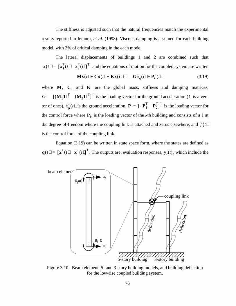
ental
ng
that
ten
ices,
c-
for
ed as
the
n
The stiffness is adjusted such that the natural frequencies match the experim
results reported in Iemura,et al. (1998). Viscous damping is assumed for each buildi
model, with 2% of critical damping in the each mode.
The lateral displacements of buildings 1 and 2 are combined such
and the equations of motion for the coupled system are writ
(3.19)
where , , and are the global mass, stiffness and damping matr
is the loading vector for the ground acceleration ( is a ve
tor of ones), is the ground acceleration, is the loading vector
the control force where is the loading vector of thekth building and consists of a 1 at
the degree-of-freedom where the coupling link is attached and zeros elsewhere, and
is the control force of the coupling link.
Equation (3.19) can be written in state space form, where the states are defin
. The outputs are: evaluation responses, , which include
xi
xj
θi=0
θj=0
i
j
Figure 3.10: Beam element, 5- and 3-story building models, and building deflectiofor the low-rise coupled building system.
beam element
5-story building 3-story building
defle
ctio
n
defle
ctio
n
coupling link
x t( ) x1T
t( ) x2T
t( )[ ]T=
Mx t( ) Cx t( ) Kx t( )+ + G xg t( )– Pf t( )+=
M C K
G M 11( )T M 21( )T[ ]T= 1
xg t( ) P P1T P2
T–[ ]T=
Pk
f t( )
q t( ) xTt( ) xT
t( )[ ]T= ye t( )
76
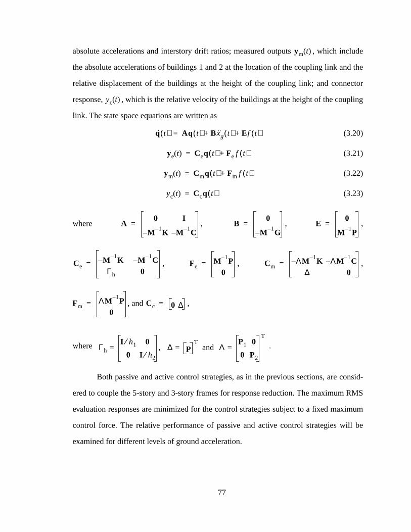
lude
d the
ctor
ling
nsid-
RMS
imum
ill be
absolute accelerations and interstory drift ratios; measured outputs , which inc
the absolute accelerations of buildings 1 and 2 at the location of the coupling link an
relative displacement of the buildings at the height of the coupling link; and conne
response, , which is the relative velocity of the buildings at the height of the coup
link. The state space equations are written as
(3.20)
(3.21)
(3.22)
(3.23)
where , , ,
, , ,
, and ,
where .
Both passive and active control strategies, as in the previous sections, are co
ered to couple the 5-story and 3-story frames for response reduction. The maximum
evaluation responses are minimized for the control strategies subject to a fixed max
control force. The relative performance of passive and active control strategies w
examined for different levels of ground acceleration.
ym t( )
yc t( )
q t( ) Aq t( ) B xg t( ) Ef t( )+ +=
ye t( ) Ceq t( ) Fe f t( )+=
ym t( ) Cmq t( ) Fm f t( )+=
yc t( ) Ccq t( )=
A0 I
M 1– K– M 1– C–= B
0
M 1– G–= E
0
M 1– P=
CeM 1– K– M 1– C–
Γh 0= Fe
M 1– P0
= CmΛM 1– K– ΛM 1– C–
∆ 0=
FmΛM 1– P
0= Cc 0 ∆=
ΓhI h1⁄ 0
0 I h2⁄,= ∆ P
Tand= Λ
P1 0
0 P2
T
=
77
es are
cceler-
xi-
kN.
egies
e been
celer-
drift
tures
e
RMS
an
/sec
solute
al 9%
r 9%
the
cou-
story
To assess the effectiveness of each control strategy, stationary RMS respons
determined for the coupled system subjected to a ground acceleration. The ground a
ation is modeled as previously defined in Section 2.4.
Efficacy of Low-Rise Coupled Building System
The system is considered for both unlimited control force and for a limited ma
mum control force. The maximum allowable RMS control force, when enforced, is 20
The three design earthquakes, from the previous section, are considered: astrong level
with RMS ground acceleration of 0.5 m/sec2, astrongerRMS ground acceleration of 1.75
m/sec2, and anextreme design earthquake of RMS ground acceleration 3.27 m/sec2.
Maximum RMS responses for the passive, active, and semiactive control strat
as well as for the uncoupled system are presented in Table 3.4. The responses hav
normalized with respect to the ground acceleration. The maximum absolute RMS ac
ations occur at the top floors of the building frames and the maximum RMS interstory
ratios occur at the first story of the building frames. If damage occurs to the struc
when the maximum RMS interstory drift ratio exceeds 1.67x10⁻³ (corresponding to a
maximum peak drift ratio of 5x10⁻³, Vision 2000 Committee, 1995), then for the low-ris
coupled building system, the uncontrolled buildings can withstand an earthquake of
acceleration up to 0.48 m/sec2. The semiactive coupled building system can withstand
earthquake of 0.72 m/sec2 before any damage might occur in the buildings.
The case of unlimited control force and a strong design earthquake of 0.5 m2
yield the same results. The semiactive control strategy can reduce maximum ab
RMS acceleration to 69% of the performance of the uncoupled response, an addition
beyond the performance of passive coupled building control, and to within a little ove
of the performance of the active control. The maximum RMS interstory drift ratio over
two buildings is not reduced as effectively as for the high-rise buildings. Semiactive
pled building control for a strong design earthquake reduces the maximum RMS inter
78
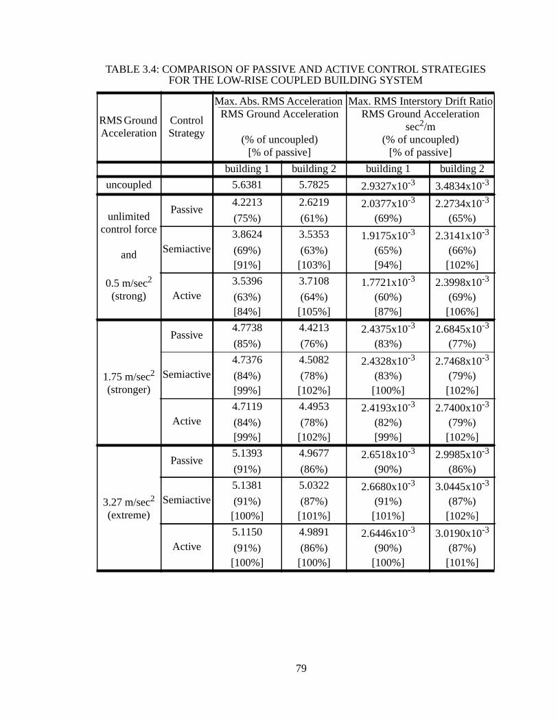
TABLE 3.4: COMPARISON OF PASSIVE AND ACTIVE CONTROL STRATEGIESFOR THE LOW-RISE COUPLED BUILDING SYSTEM
RMS GroundAcceleration
ControlStrategy
Max. Abs. RMS AccelerationRMS Ground Acceleration
(% of uncoupled)[% of passive]
Max. RMS Interstory Drift RatioRMS Ground Acceleration
sec2/m(% of uncoupled)
[% of passive]
building 1 building 2 building 1 building 2
uncoupled 5.6381 5.7825 2.9327x10⁻³ 3.4834x10⁻³
unlimitedcontrol force
and
0.5 m/sec2
(strong)
Passive4.2213 2.6219 2.0377x10⁻³ 2.2734x10⁻³
(75%) (61%) (69%) (65%)
Semiactive3.8624 3.5353 1.9175x10⁻³ 2.3141x10⁻³
(69%) (63%) (65%) (66%)[91%] [103%] [94%] [102%]
Active3.5396 3.7108 1.7721x10⁻³ 2.3998x10⁻³
(63%) (64%) (60%) (69%)[84%] [105%] [87%] [106%]
1.75 m/sec2
(stronger)
Passive4.7738 4.4213 2.4375x10⁻³ 2.6845x10⁻³
(85%) (76%) (83%) (77%)
Semiactive4.7376 4.5082 2.4328x10⁻³ 2.7468x10⁻³
(84%) (78%) (83%) (79%)[99%] [102%] [100%] [102%]
Active4.7119 4.4953 2.4193x10⁻³ 2.7400x10⁻³
(84%) (78%) (82%) (79%)[99%] [102%] [99%] [102%]
3.27 m/sec2
(extreme)
Passive5.1393 4.9677 2.6518x10⁻³ 2.9985x10⁻³
(91%) (86%) (90%) (86%)
Semiactive5.1381 5.0322 2.6680x10⁻³ 3.0445x10⁻³
(91%) (87%) (91%) (87%)[100%] [101%] [101%] [102%]
Active5.1150 4.9891 2.6446x10⁻³ 3.0190x10⁻³
(91%) (86%) (90%) (87%)[100%] [100%] [100%] [101%]
79
rfor-
f
lera-
0-1%
treme
ve and
egies
rise
pro-
lera-
posed
oach
of
s had
en-
link
ese
build-
drift ratio to 66% of the performance of the uncoupled system and 102% of the pe
mance of passive coupled building control.
For the stronger design earthquake of 1.75 m/sec2 and the extreme earthquake o
3.27 m/sec2, the semiactive control strategy can reduce maximum absolute RMS acce
tions to 84% and 91% of the performance of the uncoupled system, an additional
beyond the performance of passive coupled building control. For the stronger and ex
design earthquakes, the relative performance difference between the passive, acti
semiactive control strategies is negligible.
The relative performance of the passive, active, and semiactive control strat
for the low-rise coupled building frames is similar to what was shown for the high-
buildings.
3.6 Chapter Summary
In this chapter, two coupled building control strategies are proposed. The first
posed control strategy is the active control of coupled buildings using absolute acce
tion and relative displacement measurements for feedback control. The second pro
control strategy is semiactive coupled building control, using a clipped-optimal appr
with the active strategy as the primary controller.
Also within this chapter, the effect of building configuration on the performance
passive and active coupled building control strategies is examined. It is observed, a
been previously alluded to (Klein and Healy, 1987, Seto,et al., 1994a), that the optimal
coupled building configuration follow two guidelines. One, where the dominant frequ
cies of the two coupled buildings do not coincide, and the second, where the coupling
is not placed at the node of a dominant vibratory mode. Failing to follow both of th
guidelines leads to a reduction in the performance of the passive and active coupled
ing control strategies.
80
to a
l. For
ith
ar
nd
tion to
timal
ated
u-
ar
um
solute
yond
. For
fit in
, for
tive to
or-
ild-
s not
ontrol
hat of
con-
When building frequencies nearly match, or the coupling link is placed near
vibratory node, active control can provide improved performance over passive contro
example, for a coupled building system with a building height ratio of
(near the height ratio where the second mode of building 2 coincides w
the third mode of building 1) and a coupling link height ratio of (ne
where the coupling link is located at the node of building 2’s seco
mode), the active control strategy can reduce the maximum absolute RMS accelera
45% of the uncoupled response and up to an additional 40% beyond that of the op
passive control strategy.
The performance of the semiactive coupled building control strategy is evalu
for a coupled building system with a building height ratio of and a co
pling link height ratio of . For this system, the coupling link is located ne
a node of building 1’s third mode. The semiactive control is able to reduce the maxim
absolute RMS acceleration to between 75% and 98% of the uncoupled maximum ab
RMS acceleration for various levels of design earthquake, and to an additional 8% be
the optimal passive control strategy (for the case assuming unlimited control force)
larger design level earthquakes, semiactive control provides less additional bene
reducing the maximum absolute RMS acceleration than passive control. Additionally
the larger earthquakes, the buildings may be damaged and the performance objec
reduce maximum accelerations may be of less importance.
Two low-rise buildings are considered for coupling in order to examine if perf
mance for buildings bending in shear deformation is similar to that for the high-rise bu
ings. The buildings do not have coinciding natural frequencies, and the coupling link i
placed at the node of a dominant vibratory mode. For the system considered, active c
reduces the maximum absolute RMS story acceleration an additional 10% beyond t
the optimal passive control. This is consistent with the additional performance active
trol provides beyond passive control for high-rise building system observed.
h2 h1⁄ 0.75=
h2 h1⁄ 0.60=
hc h2⁄ 0.75=
hc h2⁄ 0.783=
h2 h1⁄ 0.90=
hc h2⁄ 0.96=
81
MS
RMS
the
addi-
ns on
ctive
sign
rol is
ontrol
ation
active
Semiactive coupled building control is shown to reduce maximum absolute R
accelerations to 75% and 41% of the uncoupled buildings and reduce the maximum
interstory drift ratios to 69% and 53% of the uncoupled buildings. It is shown that
semiactive control strategy can reduce the maximum absolute RMS acceleration an
tional 8% beyond an optimal passive control strategy. Furthermore, placing restrictio
the maximum control force reduces the overall and relative performance of the semia
control strategy. However, for certain conditions (e.g.,building configuration has coincid-
ing natural frequencies, a coupling link placed at a vibratory node, or a strong de
earthquake), the relative performance of active control beyond that of passive cont
indeed significant. Studies in this chapter have identified scenarios where active c
can provide an additional 40% reduction of the maximum absolute RMS acceler
beyond that of the optimal passive control strategy. For this reason, in Chapter 4 the
control strategy proposed in this chapter is experimentally verified.
82
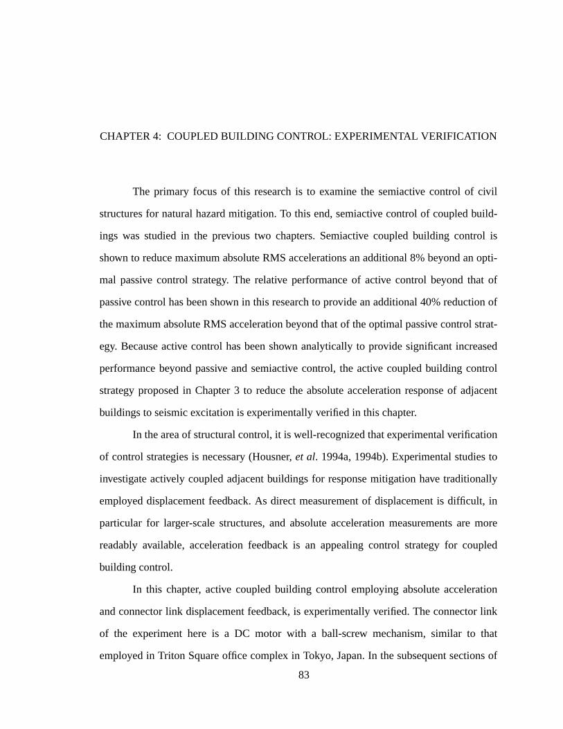
civil
uild-
ol is
opti-
at of
ion of
strat-
ased
ntrol
djacent
tion
to
nally
lt, in
more
upled
tion
r link
that
ns of
CHAPTER 4: COUPLED BUILDING CONTROL: EXPERIMENTAL VERIFICATION
The primary focus of this research is to examine the semiactive control of
structures for natural hazard mitigation. To this end, semiactive control of coupled b
ings was studied in the previous two chapters. Semiactive coupled building contr
shown to reduce maximum absolute RMS accelerations an additional 8% beyond an
mal passive control strategy. The relative performance of active control beyond th
passive control has been shown in this research to provide an additional 40% reduct
the maximum absolute RMS acceleration beyond that of the optimal passive control
egy. Because active control has been shown analytically to provide significant incre
performance beyond passive and semiactive control, the active coupled building co
strategy proposed in Chapter 3 to reduce the absolute acceleration response of a
buildings to seismic excitation is experimentally verified in this chapter.
In the area of structural control, it is well-recognized that experimental verifica
of control strategies is necessary (Housner,et al. 1994a, 1994b). Experimental studies
investigate actively coupled adjacent buildings for response mitigation have traditio
employed displacement feedback. As direct measurement of displacement is difficu
particular for larger-scale structures, and absolute acceleration measurements are
readably available, acceleration feedback is an appealing control strategy for co
building control.
In this chapter, active coupled building control employing absolute accelera
and connector link displacement feedback, is experimentally verified. The connecto
of the experiment here is a DC motor with a ball-screw mechanism, similar to
employed in Triton Square office complex in Tokyo, Japan. In the subsequent sectio
83
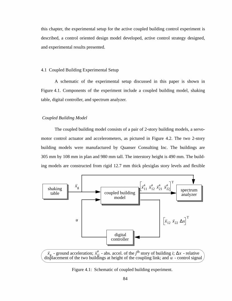
nt is
igned,
n in
king
rvo-
story
are
ild-
ible
nal
this chapter, the experimental setup for the active coupled building control experime
described, a control oriented design model developed, active control strategy des
and experimental results presented.
4.1 Coupled Building Experimental Setup
A schematic of the experimental setup discussed in this paper is show
Figure 4.1. Components of the experiment include a coupled building model, sha
table, digital controller, and spectrum analyzer.
Coupled Building Model
The coupled building model consists of a pair of 2-story building models, a se
motor control actuator and accelerometers, as pictured in Figure 4.2. The two 2-
building models were manufactured by Quanser Consulting Inc. The buildings
305 mm by 108 mm in plan and 980 mm tall. The interstory height is 490 mm. The bu
ing models are constructed from rigid 12.7 mm thick plexiglas story levels and flex
Figure 4.1: Schematic of coupled building experiment.
coupled buildingmodel
spectrumanalyzer
digitalcontroller
x12 x22 ∆xT
xg x11a
x12a
x21a
x22a
T
u
shakingtable
- ground acceleration; - abs. accel. of the jth story of buildingi; - relativedisplacement of the two buildings at height of the coupling link; and - control sig
xg xija ∆x
u
84
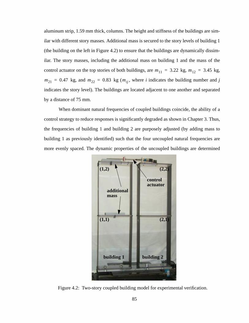
sim-
ng 1
sim-
f the
kg,
arated
of a
. Thus,
ss to
s are
ined
aluminum strip, 1.59 mm thick, columns. The height and stiffness of the buildings are
ilar with different story masses. Additional mass is secured to the story levels of buildi
(the building on the left in Figure 4.2) to ensure that the buildings are dynamically dis
ilar. The story masses, including the additional mass on building 1 and the mass o
control actuator on the top stories of both buildings, are kg,
kg, and kg ( , wherei indicates the building number andj
indicates the story level). The buildings are located adjacent to one another and sep
by a distance of 75 mm.
When dominant natural frequencies of coupled buildings coincide, the ability
control strategy to reduce responses is significantly degraded as shown in Chapter 3
the frequencies of building 1 and building 2 are purposely adjusted (by adding ma
building 1 as previously identified) such that the four uncoupled natural frequencie
more evenly spaced. The dynamic properties of the uncoupled buildings are determ
Figure 4.2: Two-story coupled building model for experimental verification.
building 1 building 2
additionalmass
controlactuator
(1,1)
(1,2)
(2,1)
(2,2)
m11 3.22= m12 3.45=
m21 0.47= m22 0.83= mij
85
uild-
crit-
ding
The
ries.
screw
. The
ow-
tenti-
d. The
the
anism.
tor is
actu-
ce-
vide
have a
m.
with the control actuator disconnected, but left in-place. The natural frequencies of b
ing 1 are 0.90 Hz and 2.70 Hz with corresponding damping ratios of 1% and 0.5% of
ical. The natural frequencies of building 2 are 1.85 Hz and 5.73 Hz with correspon
damping ratios of 1% and 0.5% of critical.
A control actuator is used to provide the forces to the coupled building system.
control actuator is pictured in Figure 4.3. The two buildings are coupled at the top sto
The actuator, manufactured by Quanser Consulting, is a DC servo-motor and ball-
mechanism with a stroke of mm, as dictated by the length of the threaded rod
stroke is limited by the distance of separation of the two buildings (75 mm). This all
able stroke is an order of magnitude larger than necessary for sufficient control. A po
ometer is attached to the motor to measure the rotation of the actuator threaded ro
relative displacement is related to the rotation of the motor through the pitch of
threaded rod attached to the servo-motor and passing through the ball-screw mech
The pitch of the threaded rod is 3.18 mm/turn. Because the servo-motor control actua
inherently open loop unstable, position feedback is employed to stabilize the control
ator. The position control of the coupling link is obtained by a PD controller with displa
ment feedback provided by the potentiometer.
PCB capacitive DC accelerometers, model 3701G3FA3G, are employed to pro
evaluation and measurement responses of the building stories. The accelerometers
Figure 4.3: Control actuator, consisting of a servo-motor with ball-screw mechanis
ball-screwmechanism
threadedrod
servo-motor
100±
86

by a
ucted
ngi-
axi-
test
e the
m the
by a
real
ig-
digi-
Real
n-
range of g and sensitivities of 1000 mV/g. The ground acceleration is measured
DC accelerometer produced by Quanser Consulting, Inc.
Shaking Table
The shaking table used is a small-scale uniaxial earthquake simulator constr
by SMI Technology and located in the Structural Dynamics and Control/Earthquake E
neering Laboratory (SDC/EEL) at the University of Notre Dame. The table has a m
mum displacement of mm and a maximum acceleration of g (with a 11.3 kg
load). The nominal operational frequency range of the simulator is 0-20 Hz. Becaus
shake table motor is inherently open loop unstable, position feedback, measured fro
shake table motor, is employed to stabilize the table. The position control is obtained
PD controller with displacement feedback.
Digital Controller
The digital controller is a PCI MultiQ I/O board1 with the WinCon realtime con-
troller2 installed in a PC. The controller is developed using Simulink and executed in
time using WinCon. The MultiQ I/O board has 13-bit analog/digital (A/D) and 12-bit d
ital/analog (D/A) converters with eight input and eight output analog channels. Four
tal encoders are also available. The Simulink code is converted to C code using the
Time Workshop in MATLAB and interfaced through the WinCon software to run the co
trol algorithms on the CPU of the PC.
1. http://www.quanser.com/english/html/solutions/fs_soln_hardware.html2. http://www.quanser.com/english/html/solutions/fs_soln_software_wincon.html
3±
120± 1±
87
ufac-
-pole
table
of
sis.
rate
ation
stem
del
s at
ine
exper-
olute
hese
ros of
a sin-
nts of
each
ment
out-
Spectrum Analyzer
The spectrum analyzer is a 4-input/2-output PC-based spectrum analyzer man
tured by DSP Technology. The device has a 90 dB signal to noise ratio and includes 8
elliptical antialiasing filters, programmable gains on the inputs/outputs, user selec
sample rates and a MATLAB user interface. These features allow for direct acquisition
high quality data and transfer functions for system identification and response analy
4.2 Experimental Coupled Building Control-Oriented Design Model
A critical precursor to the control design is the development of an accu
dynamic model of the structural system. Here, the approach used for system identific
is to construct a mathematical model to replicate the input/output behavior of the sy
(Dyke, et al. 1996a). As indicated in Figure 4.1, the inputs to the coupled building mo
are the ground acceleration ( ) and the control input to the actuator (u), and the available
outputs are the four absolute story accelerations ( , wherei indicates the building num-
ber, andj indicates the story height) and the relative displacement of the two building
the height of the coupling link ( ).
First, experimental transfer function data is obtained and curve-fit to determ
mathematical representations of the frequency responses. The transfer functions are
imentally determined from the ground acceleration and the control input to the abs
accelerations of each story and the relative displacement of the top of the buildings. T
ten experimental transfer functions are each curve-fit to determine the poles and ze
the system. Since the transfer functions represent the input/output relationships for
gle physical system, a common denominator, of 8th order, is assumed for the eleme
each column of the transfer function matrix. This corresponds to the assumption that
building is modeled with two degrees-of-freedom. Figure 4.4 compares the experi
transfer functions of the coupled building system for the absolute story acceleration
xg
xija
∆x
88
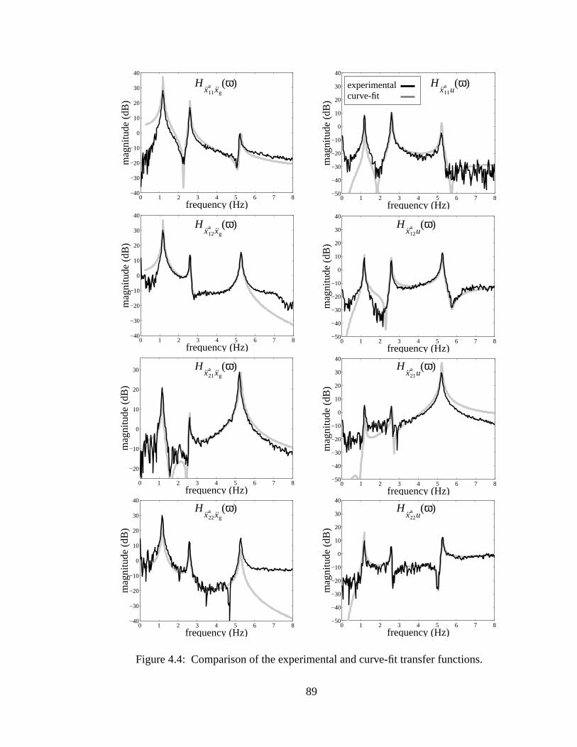
0 1 2 3 4 5 6 7 8−40
−30
−20
−10
0
10
20
30
40
mag
nitu
de (
dB)
frequency (Hz)
0 1 2 3 4 5 6 7 8−40
−30
−20
−10
0
10
20
30
40
mag
nitu
de (
dB)
frequency (Hz)
0 1 2 3 4 5 6 7 8
−20
−10
0
10
20
30
mag
nitu
de (
dB)
frequency (Hz)
0 1 2 3 4 5 6 7 8−40
−30
−20
−10
0
10
20
30
40
mag
nitu
de (
dB)
frequency (Hz)
0 1 2 3 4 5 6 7 8−50
−40
−30
−20
−10
0
10
20
30
40
mag
nitu
de (
dB)
frequency (Hz)
0 1 2 3 4 5 6 7 8−50
−40
−30
−20
−10
0
10
20
30
40
mag
nitu
de (
dB)
frequency (Hz)
0 1 2 3 4 5 6 7 8−50
−40
−30
−20
−10
0
10
20
30
40
mag
nitu
de (
dB)
frequency (Hz)
0 1 2 3 4 5 6 7 8−50
−40
−30
−20
−10
0
10
20
30
40
mag
nitu
de (
dB)
frequency (Hz)
Figure 4.4: Comparison of the experimental and curve-fit transfer functions.
Hx11
a xgω( )
Hx12
a xgω( )
Hx21
a xgω( )
Hx22
a xgω( )
Hx11
a uω( )
Hx12
a uω( )
Hx21
a uω( )
Hx22
a uω( )
experimentalcurve-fit
89
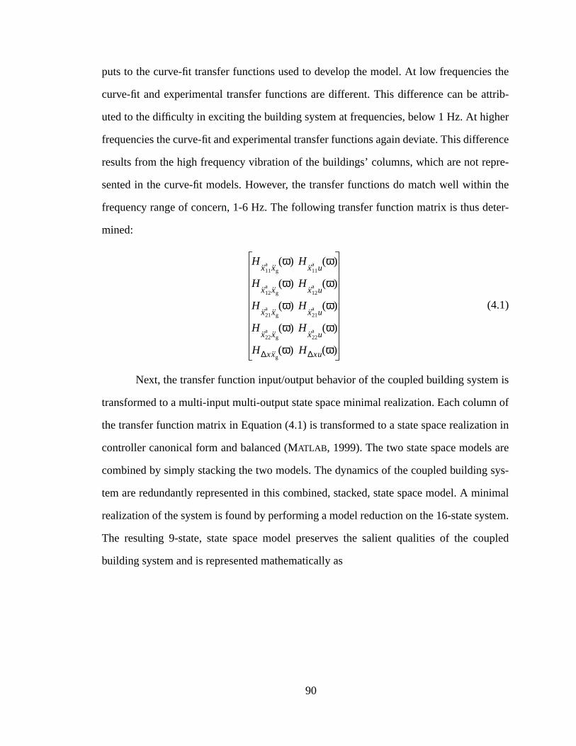
s the
ttrib-
her
rence
pre-
the
ter-
is
n of
on in
re
sys-
inimal
stem.
upled
puts to the curve-fit transfer functions used to develop the model. At low frequencie
curve-fit and experimental transfer functions are different. This difference can be a
uted to the difficulty in exciting the building system at frequencies, below 1 Hz. At hig
frequencies the curve-fit and experimental transfer functions again deviate. This diffe
results from the high frequency vibration of the buildings’ columns, which are not re
sented in the curve-fit models. However, the transfer functions do match well within
frequency range of concern, 1-6 Hz. The following transfer function matrix is thus de
mined:
(4.1)
Next, the transfer function input/output behavior of the coupled building system
transformed to a multi-input multi-output state space minimal realization. Each colum
the transfer function matrix in Equation (4.1) is transformed to a state space realizati
controller canonical form and balanced (MATLAB , 1999). The two state space models a
combined by simply stacking the two models. The dynamics of the coupled building
tem are redundantly represented in this combined, stacked, state space model. A m
realization of the system is found by performing a model reduction on the 16-state sy
The resulting 9-state, state space model preserves the salient qualities of the co
building system and is represented mathematically as
Hx11
a xgω( ) H
x11a u
ω( )
Hx12
a xgω( ) H
x12a u
ω( )
Hx21
a xgω( ) H
x21a u
ω( )
Hx22
a xgω( ) H
x22a u
ω( )
H∆xxgω( ) H∆xu ω( )
90
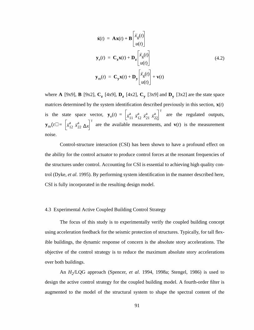
e
,
uts,
ent
t on
ies of
con-
ere,
ept
flex-
. The
tions
to
r is
of the
(4.2)
where [9x9], [9x2], [4x9], [4x2], [3x9] and [3x2] are the state spac
matrices determined by the system identification described previously in this section
is the state space vector, are the regulated outp
are the available measurements, and is the measurem
noise.
Control-structure interaction (CSI) has been shown to have a profound effec
the ability for the control actuator to produce control forces at the resonant frequenc
the structures under control. Accounting for CSI is essential to achieving high quality
trol (Dyke,et al. 1995). By performing system identification in the manner described h
CSI is fully incorporated in the resulting design model.
4.3 Experimental Active Coupled Building Control Strategy
The focus of this study is to experimentally verify the coupled building conc
using acceleration feedback for the seismic protection of structures. Typically, for tall
ible buildings, the dynamic response of concern is the absolute story accelerations
objective of the control strategy is to reduce the maximum absolute story accelera
over both buildings.
An H2/LQG approach (Spencer,et al. 1994, 1998a; Stengel, 1986) is used
design the active control strategy for the coupled building model. A fourth-order filte
augmented to the model of the structural system to shape the spectral content
x t( ) Ax t( ) Bxg t( )
u t( )+=
ye t( ) Czx t( ) Dzxg t( )
u t( )+=
ym t( ) Cyx t( ) Dyxg t( )
u t( )v t( )+ +=
A B Cz Dz Cy Dy
x t( )
ye t( ) x11a
x12a
x21a
x22a
T
=
ym t( ) x12a
x22a
∆xT
= v t( )
91
c-
ters
c-
t the
r. The
story
ontrol
kes
d
tively
the
ller.
h an
ground excitation in theH2/LQG design and analysis. This filter is the Kanai-Tajimi spe
trum with prepended filter as given in Equations (2.21) and (2.22), with parame
rad/sec and , rad/sec and . The obje
tive function is given by
(4.3)
where is a weighting matrix for the regulated outputs which is selected such tha
responses of interest are minimized and is the control signal sent to the actuato
H2/LQG control strategy is designed to minimize absolute root mean square (RMS)
accelerations over both buildings. The selection of the weighting matrixQ, which weights
a linear combination of the absolute story accelerations, determines the particular c
strategy. The optimal weighting matrix is determined iteratively and for this study ta
the form . This weighting matrix was selecte
to insure that the maximum absolute accelerations over both buildings are effec
reduced.
The resultingH2/LQG output feedback compensator is given by
(4.4)
where [13x13], [13x3] and [1x13] are the state space matrices and is
state space vector for theH2/LQG output feedback compensator.
The method of “emulation” is used for the design of the discrete-time contro
Using this technique, the continuous-time controller of Equation (4.4) is emulated wit
equivalent digital filter using a bilinear (Tustin) transformation (MATLAB , 1999). The
resulting discrete system is given by
(4.5)
ωg 1.2 2π( )= ζg 0.3= ωp 5.22 2π( )= ζp 0.2=
J1τ---E ye
T t( )Qye t( ) u2 t( )+{ } td
0
τ
∫τ ∞→lim=
Q
u t( )
Q diag 3.6633 3.8125 6.2826 4.7449=
q t( ) Acq t( ) Bcym t( )+=
u t( ) Ccq t( )=
Ac Bc Cc q t( )
q k 1+( ) Adq k( ) Bdy k( )+=
u k( ) Cdq k( )=
92
f the
screte
ing
stem
emu-
es is
ure is
of the
as
ing
B.
con-
main
build-
. Root
damp-
con-
build-
crew
m the
ero
where [13x13], [13x3] and [1x13] are the discrete state space matrices o
feedback compensator and is the discrete state space vector, is the di
measurements at thekth time step and is the discrete control signal. The sampl
rate of the controller is 0.01 sec, which is greater than 10 times the closed-loop sy
bandwidth. The equivalent discrete system adequately represents the behavior of the
lated continuous-time system over the frequency range of interest.
A consequence of modeling continuous structures with a finite number of mod
that at certain frequencies (for this experiment at frequencies above 6 Hz) the struct
not well represented by the design model. Care must be taken during the design
controller to insure sufficient roll-off of the control effort at higher frequencies.This w
accomplished by analytically determining the loop gain, from Figure 4.1, dur
the design of the controller and rejecting those controllers where d
4.4 Experimental Active Coupled Building Results
Two series of tests are conducted to evaluate the performance of the actively
trolled coupled building system subjected to ground excitation. First, a frequency do
examination is conducted whereby the transfer functions are observed. Second, the
ings are subjected to simulated earthquakes, and the time histories are considered
mean square (RMS) response reduction is observed, which illustrate the increased
ing of the active control strategy.
To provide a baseline for comparison of the active control strategy, two other
figurations are considered: the uncoupled building system and the rigidly connected
ing system. The uncoupled system is realized by simply disconnecting the s
mechanism from the actuator motor. The actuator components are not removed fro
top story of the buildings. The rigidly connected building system is realized with a z
Ad Bd Cd
q k( ) ym k( )
u k( )
Huxgω( )
Huxg62.8( ) 10–>
93
the
oise
to the
g sys-
from
or the
con-
om-
red.
root
ts the
with a
olled
4.1.
.
and
and
ant
1 by
control signal to the control actuator, which locks the motor in place, fixing
distance between the buildings’ top stories.
Frequency Domain Analysis
The coupled building system is subjected to a 10 Hz bandlimited white n
ground excitation. The frequency response functions from the ground acceleration
absolute story accelerations are measured for the actively controlled coupled buildin
tem as well as for the uncoupled and rigidly connected systems. Transfer functions
the ground acceleration to the absolute story accelerations are shown in Figure 4.5 f
uncoupled, rigidly connected and controlled building systems. The analytical active
trol transfer function is also shown in Figure 4.5. The analytically expected results c
pare reasonably well to the experimental active control transfer functions.
An measure of the performance of the active coupled building is conside
The norm of a transfer function is a measure of the upper limit of the ratio of the
mean square (RMS) of the output vector to the RMS of the input (Spencer,et al. 1994).
The norm is measured as the peak value of the transfer function and it represen
maximum RMS gain of that response. For this reason, an measure is associated
“worst case” control design. Thus, as a measure of performance for the actively contr
building configurations, the peak value of the transfer functions are indicated in Table
Both peak values for frequency ranges in the neighborhood of resonant peaks (e.g. 0-2 Hz,
2-4 Hz, and 4-8 Hz) and the maximum peak value over all frequencies are provided
When the buildings are uncoupled, the resonant peaks of building 2 (
) are larger in magnitude than the resonant peaks of building 1 (
). Rigidly connecting the two buildings has the effect of reducing the reson
peaks of building 2 by 3% and 14%, while increasing the resonant peaks of building
u t( ) 0=
H∞
H∞
H∞
H∞
Hx21
a xg
Hx22
a xgH
x11a xg
Hx12
a xg
94
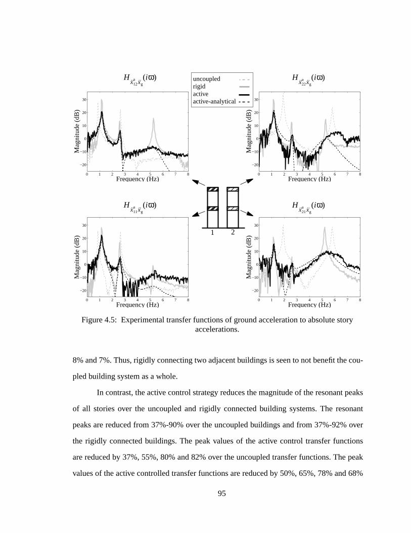
cou-
peaks
nant
over
tions
peak
68%
ry
8% and 7%. Thus, rigidly connecting two adjacent buildings is seen to not benefit the
pled building system as a whole.
In contrast, the active control strategy reduces the magnitude of the resonant
of all stories over the uncoupled and rigidly connected building systems. The reso
peaks are reduced from 37%-90% over the uncoupled buildings and from 37%-92%
the rigidly connected buildings. The peak values of the active control transfer func
are reduced by 37%, 55%, 80% and 82% over the uncoupled transfer functions. The
values of the active controlled transfer functions are reduced by 50%, 65%, 78% and
0 1 2 3 4 5 6 7 8
−20
−10
0
10
20
30
Mag
nitu
de (
dB)
Frequency (Hz)
0 1 2 3 4 5 6 7 8
−20
−10
0
10
20
30
Mag
nitu
de (
dB)
Frequency (Hz)
0 1 2 3 4 5 6 7 8
−20
−10
0
10
20
30
Mag
nitu
de (
dB)
Frequency (Hz)
0 1 2 3 4 5 6 7 8
−20
−10
0
10
20
30
Mag
nitu
de (
dB)
Frequency (Hz)
Figure 4.5: Experimental transfer functions of ground acceleration to absolute stoaccelerations.
Hx12
a xgiω( )
Hx21
a xgiω( )
Hx22
a xgiω( )
Hx11
a xgiω( )
1 2
uncoupledrigidactiveactive-analytical
95
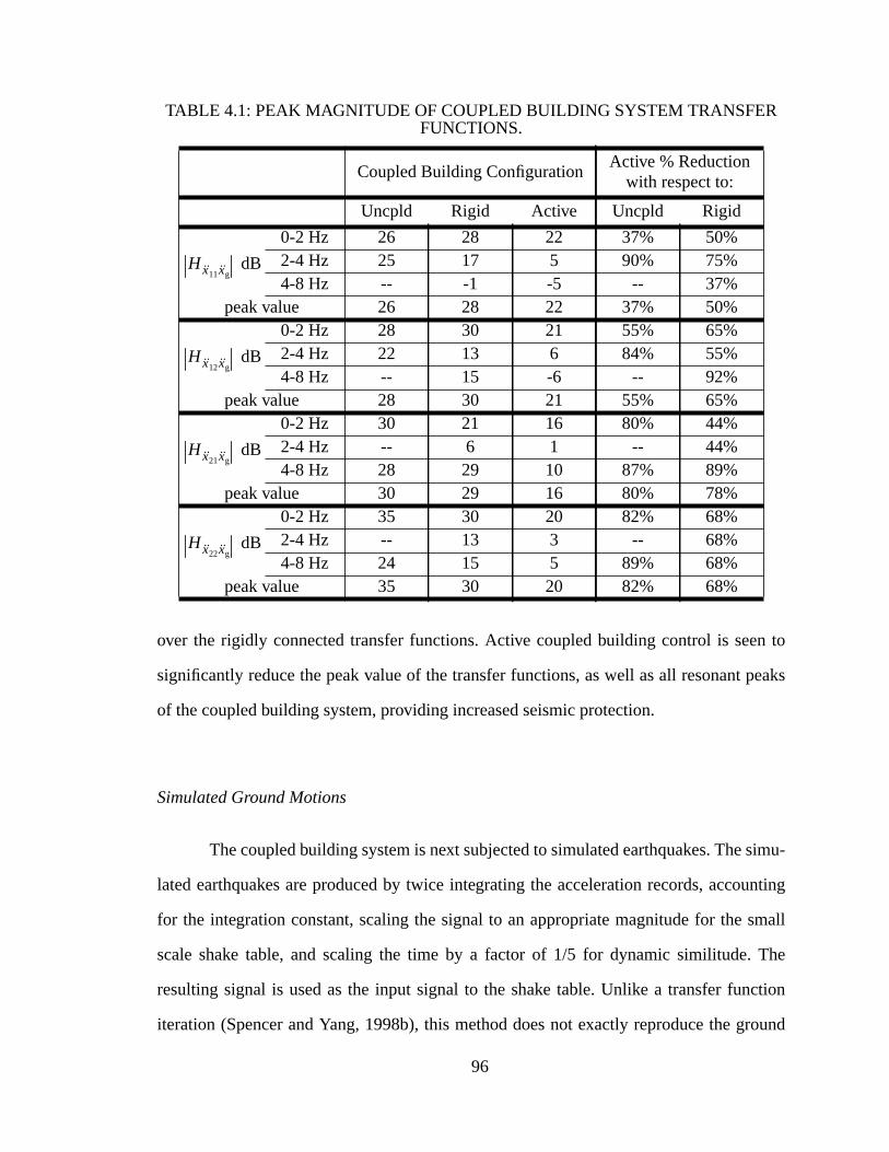
n to
peaks
simu-
unting
small
The
ction
round
over the rigidly connected transfer functions. Active coupled building control is see
significantly reduce the peak value of the transfer functions, as well as all resonant
of the coupled building system, providing increased seismic protection.
Simulated Ground Motions
The coupled building system is next subjected to simulated earthquakes. The
lated earthquakes are produced by twice integrating the acceleration records, acco
for the integration constant, scaling the signal to an appropriate magnitude for the
scale shake table, and scaling the time by a factor of 1/5 for dynamic similitude.
resulting signal is used as the input signal to the shake table. Unlike a transfer fun
iteration (Spencer and Yang, 1998b), this method does not exactly reproduce the g
TABLE 4.1: PEAK MAGNITUDE OF COUPLED BUILDING SYSTEM TRANSFERFUNCTIONS.
Coupled Building ConfigurationActive % Reduction
with respect to:
Uncpld Rigid Active Uncpld Rigid
0-2 Hz 26 28 22 37% 50%
dB 2-4 Hz 25 17 5 90% 75%4-8 Hz -- -1 -5 -- 37%
peak value 26 28 22 37% 50%0-2 Hz 28 30 21 55% 65%
dB 2-4 Hz 22 13 6 84% 55%4-8 Hz -- 15 -6 -- 92%
peak value 28 30 21 55% 65%0-2 Hz 30 21 16 80% 44%
dB 2-4 Hz -- 6 1 -- 44%4-8 Hz 28 29 10 87% 89%
peak value 30 29 16 80% 78%0-2 Hz 35 30 20 82% 68%
dB 2-4 Hz -- 13 3 -- 68%4-8 Hz 24 15 5 89% 68%
peak value 35 30 20 82% 68%
Hx11xg
Hx12xg
Hx21xg
Hx22xg
96
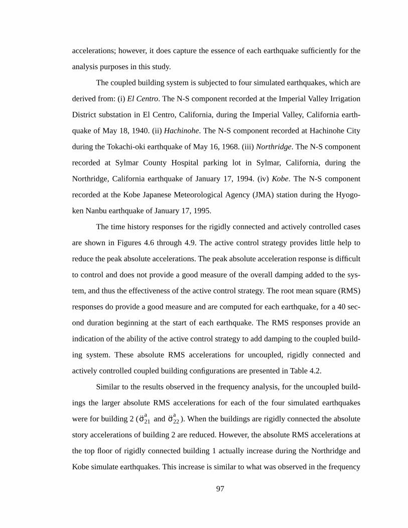
for the
h are
on
th-
ity
the
ogo-
ases
lp to
difficult
e sys-
RMS)
40 sec-
ide an
ild-
and
uild-
uakes
lute
ons at
and
uency
accelerations; however, it does capture the essence of each earthquake sufficiently
analysis purposes in this study.
The coupled building system is subjected to four simulated earthquakes, whic
derived from: (i)El Centro. The N-S component recorded at the Imperial Valley Irrigati
District substation in El Centro, California, during the Imperial Valley, California ear
quake of May 18, 1940. (ii)Hachinohe. The N-S component recorded at Hachinohe C
during the Tokachi-oki earthquake of May 16, 1968. (iii)Northridge. The N-S component
recorded at Sylmar County Hospital parking lot in Sylmar, California, during
Northridge, California earthquake of January 17, 1994. (iv)Kobe. The N-S component
recorded at the Kobe Japanese Meteorological Agency (JMA) station during the Hy
ken Nanbu earthquake of January 17, 1995.
The time history responses for the rigidly connected and actively controlled c
are shown in Figures 4.6 through 4.9. The active control strategy provides little he
reduce the peak absolute accelerations. The peak absolute acceleration response is
to control and does not provide a good measure of the overall damping added to th
tem, and thus the effectiveness of the active control strategy. The root mean square (
responses do provide a good measure and are computed for each earthquake, for a
ond duration beginning at the start of each earthquake. The RMS responses prov
indication of the ability of the active control strategy to add damping to the coupled bu
ing system. These absolute RMS accelerations for uncoupled, rigidly connected
actively controlled coupled building configurations are presented in Table 4.2.
Similar to the results observed in the frequency analysis, for the uncoupled b
ings the larger absolute RMS accelerations for each of the four simulated earthq
were for building 2 ( and ). When the buildings are rigidly connected the abso
story accelerations of building 2 are reduced. However, the absolute RMS accelerati
the top floor of rigidly connected building 1 actually increase during the Northridge
Kobe simulate earthquakes. This increase is similar to what was observed in the freq
σ21a σ22
a
97
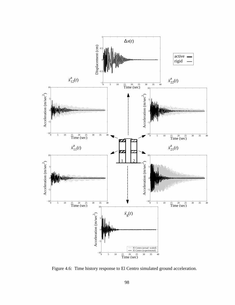
0 5 10 15 20 25 30 35 40−10
−5
0
5
10
Acc
ele
ratio
n (
m/s
ec2 )
Time (sec)
0 5 10 15 20 25 30 35 40−1
−0.5
0
0.5
1
Dis
pla
cem
en
t (c
m)
Time (sec)
0 5 10 15 20 25 30 35 40−10
−5
0
5
10
Acc
ele
ratio
n (
m/s
ec2 )
Time (sec)
0 5 10 15 20 25 30 35 40−10
−5
0
5
10
Acc
ele
ratio
n (
m/s
ec2 )
Time (sec)
El Centro (actual−scaled)El Centro (experimental)
0 5 10 15 20 25 30 35 40−10
−5
0
5
10
Acc
ele
ratio
n (
m/s
ec2 )
Time (sec)0 5 10 15 20 25 30 35 40
−10
−5
0
5
10
Acc
ele
ratio
n (
m/s
ec2 )
Time (sec)
Figure 4.6: Time history response to El Centro simulated ground acceleration.
x21a
t( )x11a
t( )
1 2
xg t( )
x22a
t( )x12a
t( )
∆x t( )
activerigid
98
.
0 5 10 15 20 25 30 35 40−10
−5
0
5
10
Acc
ele
ratio
n (
m/s
ec2 )
Time (sec)
0 5 10 15 20 25 30 35 40−1
−0.5
0
0.5
1
Dis
pla
cem
en
t (c
m)
Time (sec)
0 5 10 15 20 25 30 35 40−10
−5
0
5
10
Acc
ele
ratio
n (
m/s
ec2 )
Time (sec)
0 5 10 15 20 25 30 35 40−10
−5
0
5
10
Acc
ele
ratio
n (
m/s
ec2 )
Time (sec)
Hachinohe (actual−scaled)Hachinohe (experimental)
0 5 10 15 20 25 30 35 40−10
−5
0
5
10
Acc
ele
ratio
n (
m/s
ec2 )
Time (sec)0 5 10 15 20 25 30 35 40
−10
−5
0
5
10
Acc
ele
ratio
n (
m/s
ec2 )
Time (sec)
Figure 4.7: Time history response to Hachinohe simulated ground acceleration
x21a
t( )x11a
t( )
1 2
xg t( )
x22a
t( )x12a
t( )
∆x t( )
activerigid
99
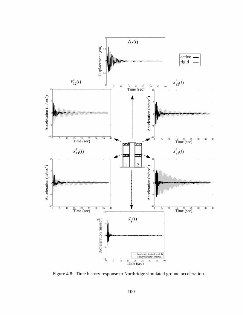
.
0 5 10 15 20 25 30 35 40−10
−5
0
5
10
Acc
ele
ratio
n (
m/s
ec2 )
Time (sec)0 5 10 15 20 25 30 35 40
−10
−5
0
5
10
Acc
ele
ratio
n (
m/s
ec2 )
Time (sec)
0 5 10 15 20 25 30 35 40−1
−0.5
0
0.5
1
Dis
pla
cem
en
t (c
m)
Time (sec)
0 5 10 15 20 25 30 35 40−10
−5
0
5
10
Acc
ele
ratio
n (
m/s
ec2 )
Time (sec)
Northridge (actual−scaled)Northridge (experimental)
0 5 10 15 20 25 30 35 40−10
−5
0
5
10
Acc
ele
ratio
n (
m/s
ec2 )
Time (sec)0 5 10 15 20 25 30 35 40
−10
−5
0
5
10
Acc
ele
ratio
n (
m/s
ec2 )
Time (sec)
Figure 4.8: Time history response to Northridge simulated ground acceleration
x21a
t( )x11a
t( )
1 2
xg t( )
x22a
t( )x12a
t( )
∆x t( )
activerigid
100
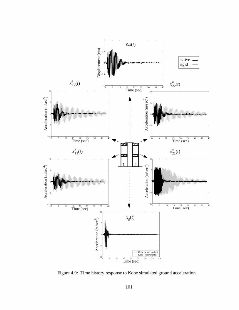
0 5 10 15 20 25 30 35 40−1
−0.5
0
0.5
1
Dis
plac
emen
t (cm
)
Time (sec)
0 5 10 15 20 25 30 35 40−10
−5
0
5
10
Acc
eler
atio
n (m
/sec2 )
Time (sec)
Kobe (actual−scaled)Kobe (experimental)
0 5 10 15 20 25 30 35 40−10
−5
0
5
10
Acc
eler
atio
n (m
/sec2 )
Time (sec)
0 5 10 15 20 25 30 35 40−10
−5
0
5
10
Acc
eler
atio
n (m
/sec2 )
Time (sec)
0 5 10 15 20 25 30 35 40−10
−5
0
5
10
Acc
eler
atio
n (m
/sec2 )
Time (sec)
0 5 10 15 20 25 30 35 40−10
−5
0
5
10
Acc
eler
atio
n (m
/sec2 )
Time (sec)
Figure 4.9: Time history response to Kobe simulated ground acceleration.
x21a
t( )x11a
t( )
1 2
xg t( )
x22a
t( )x12a
t( )
∆x t( )
activerigid
101
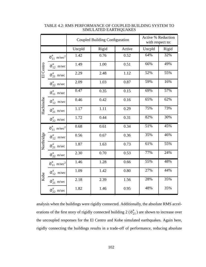
cel-
over
here,
lute
analysis when the buildings were rigidly connected. Additionally, the absolute RMS ac
erations of the first story of rigidly connected building 2 ( ) are shown to increase
the uncoupled responses for the El Centro and Kobe simulated earthquakes. Again
rigidly connecting the buildings results in a trade-off of performance, reducing abso
TABLE 4.2: RMS PERFORMANCE OF COUPLED BUILDING SYSTEM TOSIMULATED EARTHQUAKES
Coupled Building ConfigurationActive % Reduction
with respect to:
Uncpld Rigid Active Uncpld Rigid
El C
entr
o
m/sec2 1.42 0.76 0.52 64% 32%
m/sec 1.49 1.00 0.51 66% 49%
m/sec 2.29 2.48 1.12 52% 55%
m/sec 2.09 1.03 0.87 59% 16%
Hac
hino
he
m/sec0.47 0.35 0.15 69% 57%
m/sec 0.46 0.42 0.16 65% 62%
m/sec 1.17 1.11 0.29 75% 73%
m/sec 1.72 0.44 0.31 82% 30%
Nor
thrid
ge
m/sec2 0.68 0.61 0.34 51% 45%
m/sec 0.56 0.67 0.36 35% 46%
m/sec 1.87 1.63 0.73 61% 55%
m/sec 2.30 0.70 0.53 77% 24%
Kob
e
m/sec2 1.46 1.28 0.66 55% 48%
m/sec 1.09 1.42 0.80 27% 44%
m/sec 2.18 2.39 1.56 28% 35%
m/sec 1.82 1.46 0.95 48% 35%
σ11a
σ12a
σ21a
σ22a
σ11a
σ12a
σ21a
σ22a
σ11a
σ12a
σ21a
σ22a
σ11a
σ12a
σ21a
σ22a
σ21a
102
ration
le.
ions.
rations
idly
s the
by 30-
ctive
oupled
u-
igidly
seen
nses
ding
of the
due to
ism,
ntrol
p of the
the
del to
acceleration responses at some stories while increasing the absolute accele
responses at other stories, thus not benefiting the coupled building system as a who
The active control strategy is able to reduce all of the absolute RMS accelerat
The active control strategy reduces the RMS responses of the absolute story accele
by 52-66% over the uncoupled buildings and by an additional 16-55% over the rig
connected buildings for the El Centro simulated earthquake. Active control reduce
absolute RMS acceleration responses by 65-82% over the uncoupled buildings and
73% over the rigidly connected buildings for the Hachinohe simulated earthquake. A
control reduces the absolute RMS acceleration responses by 35-77% over the unc
buildings and by 24-55% over the rigidly connected buildings for the Northridge sim
lated earthquake and 27-55% over the uncoupled buildings and 35-48% over the r
connected buildings for the Kobe simulated earthquake. The active control strategy is
to significantly reduce all of the coupled building system’s absolute acceleration respo
to four different simulated historical earthquakes.
4.5 Chapter Summary
This chapter details experimental tests conducted on two 2-story flexible buil
models, placed adjacent to one another on a shake table and coupled at the top
building models with a control actuator, to reduce absolute acceleration responses
seismic excitation. The control actuator is a DC servo-motor with a ball screw mechan
similar to the 35-ton control actuators coupling the Triton Square buildings. The co
design uses absolute acceleration and relative displacement measurements at the to
building models, where the actuator is located.
A control-oriented design model is developed by experimentally measuring
transfer functions of the coupled building system and developing a mathematical mo
103
s for
. The
func-
f the
rigidly
ulated
oupled
8% of
rigidly
rela-
lly to
replicate the input/output behavior of the system. This design model fully account
control-structure interaction.
Frequency and time domain analyses are performed for system evaluation
active coupled building system is able to reduce the resonant peaks of the transfer
tions of absolute story acceleration to ground acceleration to between 67-18% o
uncoupled system’s resonant peaks and corresponding to between 50-88% over the
connected resonant peaks. The coupled building system is subjected to four sim
earthquakes and absolute RMS story accelerations are computed. The active c
building system can reduce these absolute RMS story accelerations to as low as 1
the uncoupled absolute RMS accelerations and to as low as 73% compared to the
connected system. Active control, using readily available absolute acceleration and
tive displacement feedback measurements of the coupling link, is shown experimenta
be an effective method of structural control.
104
, sus-
al exci-
s are
on.
f the
988).
the
ration
iced
uch as
ing
ve and
been
925).
ctural
d full-
posed
-
erifies
CHAPTER 5: CABLE DAMPING CONTROL: BACKGROUND
Cables are efficient structural elements that are used in cable-stayed bridges
pension bridges and other cable structures. These cables are subject to environment
tations, such as rain-wind induced vibration, and support excitations. Steel cable
flexible and have low inherent damping, resulting in high susceptibility to vibrati
Vibration can result in premature cable or connection failure and/or breakdown o
cable corrosion protection systems, reducing the life of the cable structure (Watson, 1
Additionally, cable vibrations can have a detrimental effect on public confidence in
safety of cable structures. Transmission lines have also demonstrated significant vib
problems, including those caused by vortex shedding, wake-induced oscillation, and
and ice-free galloping. Fatigue of the transmission lines near clamps or masses (s
aircraft warning spheres) is the principal effect of conductor vibration, though gallop
can cause sparkover between lines of different phase (Tunstall, 1997).
Cable damping, as studied herein, uses transversely attached passive, acti
semiactive dampers to mitigate cable vibration. Suppressing cable vibration has
done, on transmission lines, since the first part of the last century (Stockbridge, 1
However, cable damping employing transversely attached dampers to the cable stru
elements of civil structures is more recent, in fact only over the past two decades.
Numerous passive and active cable damping studies have been performed an
scale applications realized. Semiactive control of a taut cable has recently been pro
(Johnsonet al., 1999, 2000a, and 2000b, Bakeret al. 1999a, and Baker 1999b). This dis
sertation extends the semiactive analytical studies to include cables with sag and v
experimentally cable damping.
105
trol-
able
iactive
stay
e and
cables
ncies
tics of
viron-
and
s are
uned
mping
mis-
nduc-
mpers
mper
iscous
s for
iscous
l fre-
In this chapter a literature review of cable damping control is presented, a con
oriented evaluation model for the in-plane motion of cables with sag is developed, c
excitation and a performance measure are identified, and passive, active and sem
cable damping control strategies presented.
5.1 Cable Damping Literature Review
A number of methods have been proposed to mitigate cable vibrations. For
cables, tying cables together, aerodynamic cable surface modification, and passiv
active axial and transverse cable control have been used to dampen vibration. Tying
together shortens the effective length of the cables, and is intended to shift the freque
of the cable out of the range of the excitation. This strategy deteriorates the aesthe
the cable structure. Changing the surface of the cable to reduce susceptibility to en
mental excitations has also been explored, but is impractical for retrofit applications
may increase motion during high winds. For transmission lines, two primary method
used for reducing vibration. Stockbridge dampers (Stockbridge, 1925), a variety of t
vibration absorbers, are the most common means today for adding supplemental da
to transmission lines (Tunstall, 1997). An alternate solution for multiple parallel trans
sion lines is adding dampers to the bundle spacers routinely used for separating co
tors (Edwards and Boyd, 1965).
Various researchers have proposed passive control of cables using viscous da
attached transverse to the cables. Kovacs (1982) first identified that an optimal da
size exists and developed optimal damping coefficients for the transverse passive v
damper control strategy of a taut cable. Sulekh (1990) and Pachecoet al. (1993) numeri-
cally developed a “universal” design curve to facilitate the design of passive damper
stay cables. This nondimensionalized curve can be used to determine the optimal v
damping properties for a desired mode of any given cable span and fundamenta
106
effi-
that,
ately
tions,
Sky-
89).
c and
an
may
rain-
els of
and
nsion
0 to
e level
cable
apidly
most
with
that
ts the
sym-
quency. Krenk (1999) obtained explicit asymptotic results for the optimal damping co
cients, developing an analytical solution for the design curve. These studies indicate
for a passive linear damper, the maximum supplemental damping ratio is approxim
/2L, where is the distance from the cable anchorage to the damper andL is the
length of the cable.
Transverse passive viscous dampers have been applied to full-scale applica
including the cables on the Brotonne Bridge in France (Gimsing, 1983), the Sunshine
way Bridge in Florida (Watson, 1988) and the Aratsu Bridge in Japan (Yoshimura, 19
The damper location is typically restricted to be close to the bridge deck for aestheti
practical reasons. For short cables, a high /L ratio is feasible and a passive damper c
provide sufficient damping. For increasingly longer bridge cables, passive dampers
not provide enough supplemental damping to eliminate vibration effects, such as
wind induced motion, without significant changes to the aesthetics of the structure.
Several recent papers have shown that semiactive dampers may provide lev
damping far superior to their passive counterparts. Johnsonet al. (1999, 2000a, 2000b)
and Bakeret al. (1999a, 1999b) used a taut string model of in-plane cable vibration
developed a control-oriented model using a static deflection shape in a series expa
for the cable motion. They showed that a “smart” semiactive damper can provide 5
80% reduction in cable response compared to the optimal passive linear damper. Th
of reduction was most significant when the damper was connected close to the
anchorage. A passive damper moved close to the end of the cable was shown to r
lose any ability to add damping to the system, whereas a semiactive damper retained
of its performance even at damper locations below 1% of the cable length (though
larger forces).
The taut string model of cable vibration neglects some cable characteristics
are known to have some effect on passive damper performance. Cable sag effec
dynamics of the cable. In particular, sag modifies the stiffness of the modes that are
xd xd
xd
107
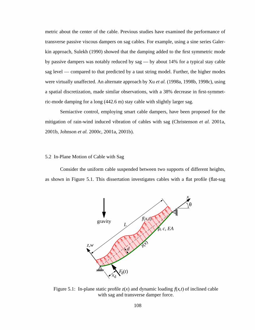
nce of
s Galer-
mode
cable
odes
met-
r the
ights,
t-sag
metric about the center of the cable. Previous studies have examined the performa
transverse passive viscous dampers on sag cables. For example, using a sine serie
kin approach, Sulekh (1990) showed that the damping added to the first symmetric
by passive dampers was notably reduced by sag — by about 14% for a typical stay
sag level — compared to that predicted by a taut string model. Further, the higher m
were virtually unaffected. An alternate approach by Xuet al.(1998a, 1998b, 1998c), using
a spatial discretization, made similar observations, with a 38% decrease in first-sym
ric-mode damping for a long (442.6 m) stay cable with slightly larger sag.
Semiactive control, employing smart cable dampers, have been proposed fo
mitigation of rain-wind induced vibration of cables with sag (Christensonet al. 2001a,
2001b, Johnsonet al. 2000c, 2001a, 2001b).
5.2 In-Plane Motion of Cable with Sag
Consider the uniform cable suspended between two supports of different he
as shown in Figure 5.1. This dissertation investigates cables with a flat profile (fla
Figure 5.1: In-plane static profilez(x) and dynamic loadingf(x,t) of inclined cablewith sag and transverse damper force.
ρ, c, EA
z,w
x
L
θ
f(x,t)
d
xdFd(t)
gravity
z(x)
108
s than
vine,
n ratio
f longi-
he
otion
tion
-
and
lane
en-
bars,
taut
the
rvine,
cables); for a horizontal cable, this assumption requires the sag to span ratio be les
1:8 (for inclined cables the assumption is valid but over a smaller range of sag) (Ir
1981). The primary suspension cables for the Golden Gate Bridge have a sag to spa
of less than 1:8 and can thus be considered as flat-sag cables. Further, the effects o
tudinal flexibility are included and flexural rigidity is ignored. The static profile of t
cable can be approximated by a parabolic curve and the in-plane transverse cable m
, relative to the static profile, is given by the nondimensional equation of mo
(Irvine, 1981)
(5.1)
in the domain , with boundary conditions . is the vis
cous damping per unit length, and denote partial derivatives with respect to
, respectively, is the distributed load on the cable, is a transverse in-p
damper force at location , and is the Dirac delta function. The nondim
sional quantities are related to their dimensional counterparts, shown with over
according to the following relations
whereL is the length of the cable, is the fundamental natural frequency of the
cable,H is the component of cable tension in the longitudinal x-direction, and is
cable mass per unit length. is the nondimensional independent parameter (I
1981)
(5.2)
where is the inclination angle, is the static (stretched) length of the cable
w x t,( )
w x t,( ) cw x t,( )1π2-----w″ x t,( )–
λ2
π2----- w ξ t,( ) ξd
0
1
∫+ + f x t,( ) Fd t( )δ x xd–( )+=
0 x 1≤ ≤ w 0 t,( ) w 1 t,( ) 0= = c
( )′ ˙( ) x
t f x t,( ) Fd t( )
x xd= δ ·( )
t ω0t= x x L⁄= c c ρω0⁄= w x t,( ) w x t,( ) L⁄= ω02 Hπ2 ρL2⁄=
δ x xd–( ) Lδ x xd–( )= f x t,( ) L f x t,( ) π2H⁄= Fd t( ) Fd t( ) π2H⁄=
ω0
ρ
λ2
λ2 ρgL θcosH
---------------------- 2 EAL
HLe----------- 64
dL---
2EALHLe-----------= =
θ Le
109
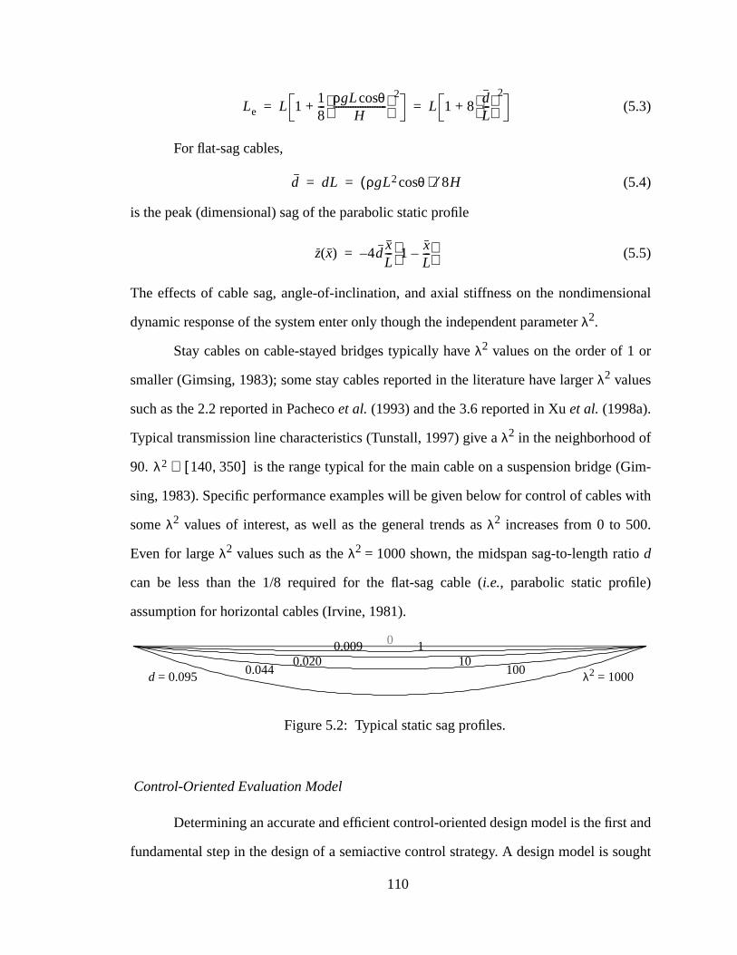
ional
im-
with
t and
ought
(5.3)
For flat-sag cables,
(5.4)
is the peak (dimensional) sag of the parabolic static profile
(5.5)
The effects of cable sag, angle-of-inclination, and axial stiffness on the nondimens
dynamic response of the system enter only though the independent parameterλ2.
Stay cables on cable-stayed bridges typically haveλ2 values on the order of 1 or
smaller (Gimsing, 1983); some stay cables reported in the literature have largerλ2 values
such as the 2.2 reported in Pachecoet al. (1993) and the 3.6 reported in Xuet al. (1998a).
Typical transmission line characteristics (Tunstall, 1997) give aλ2 in the neighborhood of
90. is the range typical for the main cable on a suspension bridge (G
sing, 1983). Specific performance examples will be given below for control of cables
someλ2 values of interest, as well as the general trends asλ2 increases from 0 to 500.
Even for largeλ2 values such as theλ2 = 1000 shown, the midspan sag-to-length ratiod
can be less than the 1/8 required for the flat-sag cable (i.e., parabolic static profile)
assumption for horizontal cables (Irvine, 1981).
Control-Oriented Evaluation Model
Determining an accurate and efficient control-oriented design model is the firs
fundamental step in the design of a semiactive control strategy. A design model is s
Le L 118--- ρgL θcos
H----------------------
2+ L 1 8
dL---
2
+= =
d dL ρgL2 θcos( ) 8H⁄= =
z x( ) 4dxL--- 1 x
L---–
–=
λ2 140 350,[ ]∈
Figure 5.2: Typical static sag profiles.
1
λ2 = 100010010
0
d = 0.095 0.0440.020
0.009
110
mber
have
in the
quire
s
ntrol
ontrol
lower
o the
nite
ctions
ound-
con-
tatic
nver-
ere as
tion
ith a
that can capture the salient features of the dynamic system with a relatively small nu
of degrees-of-freedom (DOFs). Previous transversely-controlled cable models
employed the Galerkin method, using only sine shape functions requiring 350 terms
series (Sulekh, 1990), as well as hybrid-type finite element methods which also re
numerous DOFs to insure accurate results (Xuet al., 1998a). Semiactive control design, a
well as the computation of performance criteria through simulation with numerous co
strategies, is impractical for systems of such size. Thus, successful semiactive c
design is dependant on determining a lower order, control-oriented design model. A
order model is accomplished here by including a static deflection shape in addition t
sine series in the approximation of the cable motion (Johnsonet al., 1999).
Using a Galerkin method, the motion of the cable may be computed using a fi
series approximation
(5.6)
where the are generalized displacements and the are a set of shape fun
that are continuous with piecewise continuous slope and that satisfy the geometric b
ary conditions
(5.7)
A sine series may be used for the shape functions, though Johnsonet al. (2000a,b)
showed that the convergence of this series is slow, making it difficult to construct a
trol-oriented model. However, they also demonstrated that the introduction of a s
deflection shape as an additional shape function significantly improved the series co
gence and provided an excellent control-oriented model. This approach is used h
well, though it must be extended to account for cable sag.
Consider the static deflection of a cable with sag due to a unit load at loca
— the same as the equation of motion (5.1) without the dynamic terms and w
unit point load on the right hand side
w x t,( ) φj x( )qj
t( )j 1=
m
∑=
qj t( ) φj x( )
φj 0( ) φj 1( ) 0= =
x xd=
111
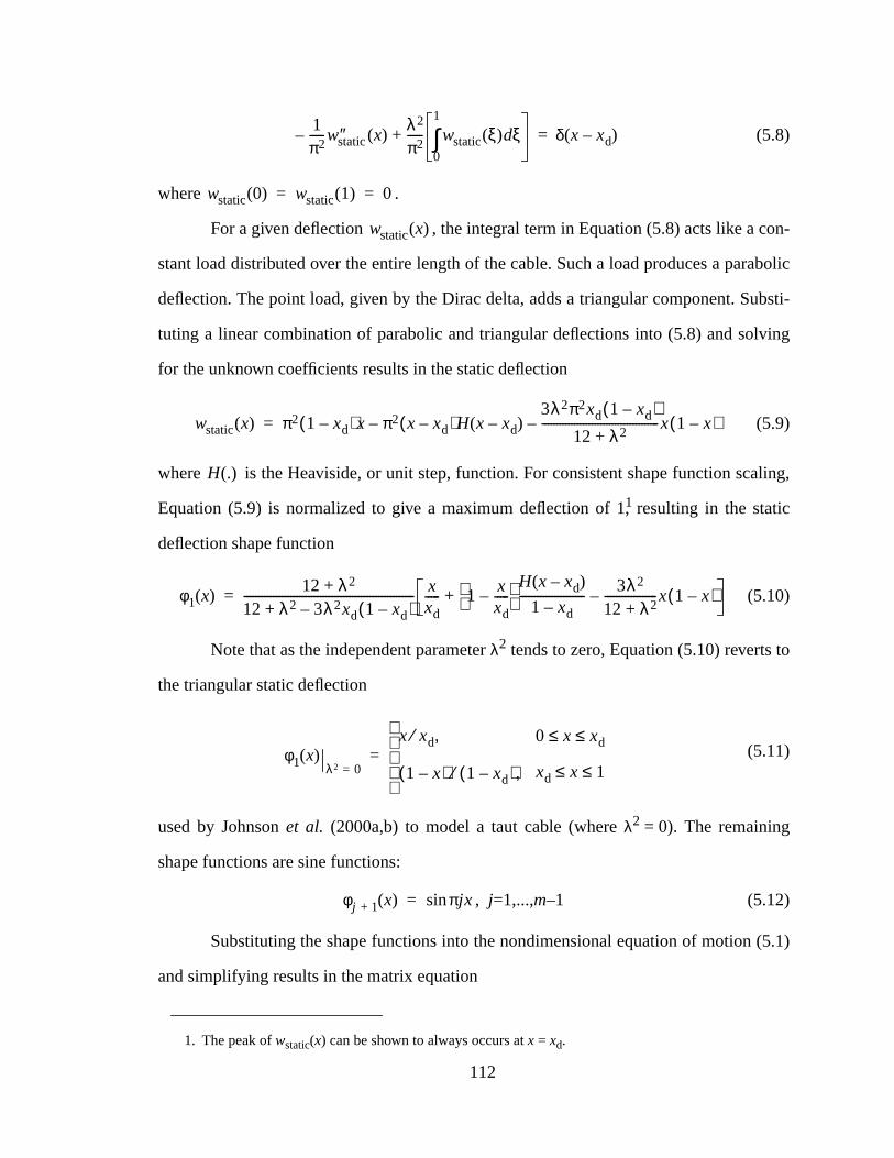
on-
abolic
bsti-
ving
ling,
o
(5.1)
(5.8)
where .
For a given deflection , the integral term in Equation (5.8) acts like a c
stant load distributed over the entire length of the cable. Such a load produces a par
deflection. The point load, given by the Dirac delta, adds a triangular component. Su
tuting a linear combination of parabolic and triangular deflections into (5.8) and sol
for the unknown coefficients results in the static deflection
(5.9)
where is the Heaviside, or unit step, function. For consistent shape function sca
Equation (5.9) is normalized to give a maximum deflection of 11, resulting in the static
deflection shape function
(5.10)
Note that as the independent parameterλ2 tends to zero, Equation (5.10) reverts t
the triangular static deflection
(5.11)
used by Johnsonet al. (2000a,b) to model a taut cable (whereλ2 = 0). The remaining
shape functions are sine functions:
, j=1,...,m–1 (5.12)
Substituting the shape functions into the nondimensional equation of motion
and simplifying results in the matrix equation
1. The peak ofwstatic(x) can be shown to always occurs atx = xd.
1π2-----wstatic″ x( )–
λ2
π2----- wstatic ξ( ) ξd
0
1
∫+ δ x xd–( )=
wstatic 0( ) wstatic 1( ) 0= =
wstatic x( )
wstatic x( ) π2 1 xd–( )x π2 x xd–( )H x xd–( )–3λ2π2xd 1 xd–( )
12 λ2+----------------------------------------x 1 x–( )–=
H .( )
φ1 x( )12 λ2+
12 λ2 3λ2xd 1 xd–( )–+---------------------------------------------------------- x
xd----- 1 x
xd-----–
H x xd–( )
1 xd–---------------------- 3λ2
12 λ2+------------------x 1 x–( )–+=
φ1 x( )λ2 0=
x xd⁄ , 0 x xd≤ ≤
1 x–( ) 1 x– d( )⁄ , xd x 1≤ ≤
=
φj 1+ x( ) πjxsin=
112
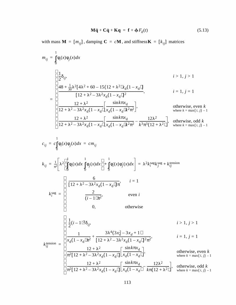
(5.13)
with mass , damping , and stiffness matrices
Mq Cq Kq+ + f f Fd t( )+=
M mij[ ]= C cM= K kij[ ]=
mij φi x( )φj x( ) xd0
1
∫=
12---δij , i > 1 j > 1,
48 130------λ2 4λ2 60 15 12 λ2+( )xd 1 xd–( )–+[ ]+
12 λ2 3λ2xd 1 xd–( )–+[ ]2-------------------------------------------------------------------------------------------------------------, i = 1 j = 1,
12 λ2+12 λ2 3λ2xd 1 xd–( )–+----------------------------------------------------------
kπxdsin
xd 1 xd–( )k2π2------------------------------------ , otherwise evenk,
wherek = max i j,{ } 1–
12 λ2+12 λ2 3λ2xd 1 xd–( )–+----------------------------------------------------------
kπxdsin
xd 1 xd–( )k2π2------------------------------------ 12λ2
k3π3 12 λ2+( )----------------------------------– , otherwise oddk,
wherek = max i j,{ } 1–
=
cij c φi x( )φj x( ) xd0
1
∫ cmij= =
kij1π2----- λ2 φi x( ) xd
0
1
∫ φj x( ) xd0
1
∫
φi′ x( )φj
′ x( ) xd0
1
∫+ λ2kisagkj
sag kijtension+= =
kisag
612 λ2 3λ2xd 1 xd–( )–+[ ]π
------------------------------------------------------------------, i = 1
2i 1–( )π2
---------------------, eveni
0, otherwise
=
kijtension
12--- i 1–( )2δij , i > 1 j > 1,
1xd 1 xd–( )π2------------------------------
3λ4 3xd2 3xd– 1+( )
12 λ2 3λ2xd 1 xd–( )–+[ ]2π2-----------------------------------------------------------------------+ , i = 1 j = 1,
12 λ2+π2 12 λ2 3λ2xd 1 xd–( )–+[ ]--------------------------------------------------------------------
kπxdsin
xd 1 xd–( )------------------------ , otherwise evenk,
wherek = max i j,{ } 1–
12 λ2+π2 12 λ2 3λ2xd 1 xd–( )–+[ ]--------------------------------------------------------------------
kπxdsin
xd 1 xd–( )------------------------ 12λ2
kπ 12 λ2+( )-----------------------------– , otherwise oddk,
wherek = max i j,{ } 1–
=
113
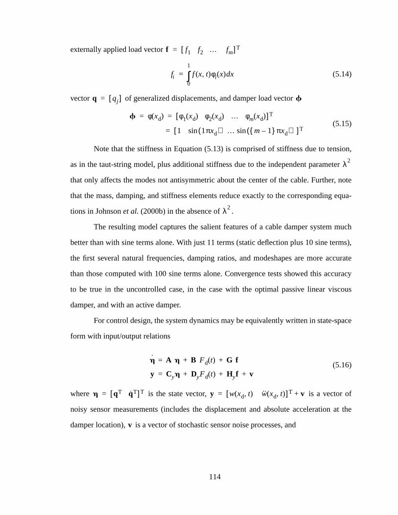
ion,
er
, note
equa-
much
rms),
ccurate
curacy
cous
pace
f
at the
externally applied load vector
(5.14)
vector of generalized displacements, and damper load vector
(5.15)
Note that the stiffness in Equation (5.13) is comprised of stiffness due to tens
as in the taut-string model, plus additional stiffness due to the independent paramet
that only affects the modes not antisymmetric about the center of the cable. Further
that the mass, damping, and stiffness elements reduce exactly to the corresponding
tions in Johnsonet al. (2000b) in the absence of .
The resulting model captures the salient features of a cable damper system
better than with sine terms alone. With just 11 terms (static deflection plus 10 sine te
the first several natural frequencies, damping ratios, and modeshapes are more a
than those computed with 100 sine terms alone. Convergence tests showed this ac
to be true in the uncontrolled case, in the case with the optimal passive linear vis
damper, and with an active damper.
For control design, the system dynamics may be equivalently written in state-s
form with input/output relations
(5.16)
where is the state vector, is a vector o
noisy sensor measurements (includes the displacement and absolute acceleration
damper location), is a vector of stochastic sensor noise processes, and
f f1 f2 … fm[ ]T=
fi f x t,( )φi x( ) xd0
1
∫=
q qj[ ]= f
f φ xd( ) φ1 xd( ) φ2 xd( ) … φm xd( )[ ]T= =
1 1πxd( )sin … m 1–{ }πxd( )sin[ ]T=
λ2
λ2
h = Azh + BzFd t( ) + Gzf
y = Cyh + DyFd t( ) + Hyf + v
h qT qT[ ]T= y w xd t,( ) w xd t,( )[ ]T v+=
v
114
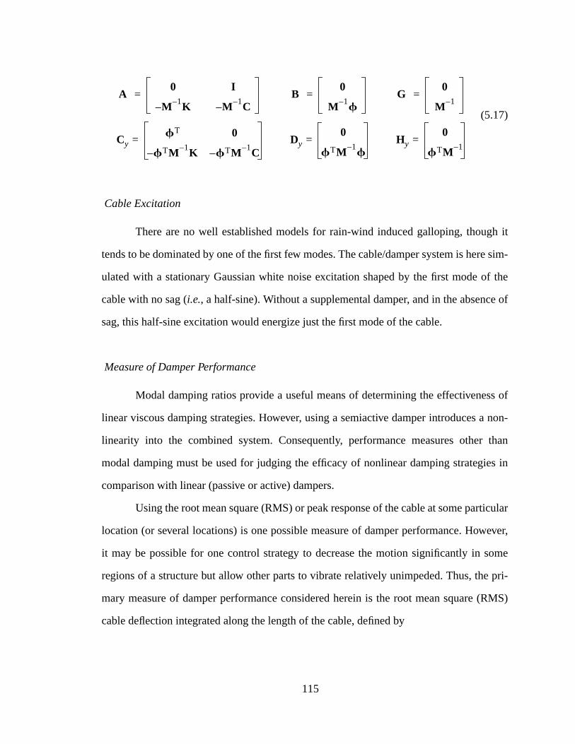
h it
e sim-
f the
e of
s of
a non-
than
es in
ticular
ever,
ome
pri-
(RMS)
(5.17)
Cable Excitation
There are no well established models for rain-wind induced galloping, thoug
tends to be dominated by one of the first few modes. The cable/damper system is her
ulated with a stationary Gaussian white noise excitation shaped by the first mode o
cable with no sag (i.e., a half-sine). Without a supplemental damper, and in the absenc
sag, this half-sine excitation would energize just the first mode of the cable.
Measure of Damper Performance
Modal damping ratios provide a useful means of determining the effectivenes
linear viscous damping strategies. However, using a semiactive damper introduces
linearity into the combined system. Consequently, performance measures other
modal damping must be used for judging the efficacy of nonlinear damping strategi
comparison with linear (passive or active) dampers.
Using the root mean square (RMS) or peak response of the cable at some par
location (or several locations) is one possible measure of damper performance. How
it may be possible for one control strategy to decrease the motion significantly in s
regions of a structure but allow other parts to vibrate relatively unimpeded. Thus, the
mary measure of damper performance considered herein is the root mean square
cable deflection integrated along the length of the cable, defined by
Az0 I
M 1– K– M 1– C–= Bz
0
M 1– f= Gz
0
M 1–=
CyfT 0
fTM 1– K– fTM 1– C–= Dy
0
fTM 1– f= Hy
0
fTM 1–=
115
ing
ance
inter-
t have
988;
ained
trol
rce is
ional
(5.18)
where is a square symmetric matrix such that . The correspond
RMS cable velocity may be computed from the generalized velocities
(5.19)
For stationary response to a stationary stochastic excitation, these perform
measures are not functions of time, but become constants.
5.3 Cable Damping Control Strategies
Three types of dampers are considered in this study. The damper of primary
est is a general semiactive device, one that may exert any requireddissipativeforce. How-
ever, comparison with passive linear viscous dampers, similar to the oil dampers tha
been installed in numerous cable-stayed bridges (Gimsing, 1983; Watson, 1
Yoshimura, 1989), is considered to demonstrate the improvements that may be g
with semiactive damping technology. Additionally, comparison with active con
devices is useful as they bound the achievable performance.
Passive Viscous Damper
If the damping device is a passive linear viscous damper, then the damper fo
(5.20)
where is a nondimensional damping constant, and is the nondimens
velocity at the damper location
σdisplacementt( ) E v2 x t,( ) xd0
1
∫ E qT t( )Mq t( )[ ]= =
trace M 1 2/ E q t( )qT t( )[ ]M 1 2/{ }=
M 1 2/ M 1 2/ M 1 2/ M=
σvelocity t( ) E qT t( )Mq t( )[ ] trace M 1 2/ E q t( )qT t( )[ ]M 1 2/{ }= =
Fd t( ) cdw xd t,( )–=
cd w xd t,( )
116
lysis.
de the
ch to
is an
tively
of
,
n
(5.21)
The modal damping may be determined via a straightforward eigenvalue ana
Note that the optimal passive damper supplies pure damping; stiffness tends to degra
damper performance (Sulekh, 1990; Xuet al., 1998b).
Active Damper
The optimal passive viscous damper provides one benchmark against whi
judge semiactive dampers. The other end of the spectrum of control possibilities
ideal active damper, which may exert any desired force. The performance of the ac
controlled systems give a performance target for semiactive control.
One family ofH2/LQG control designs is considered in this study. This family
controllers performed well for cables with (Johnsonet al., 2000a,b). These con-
trollers use force proportional to an estimate of the state of the system,
where is the feedback gain that minimizes the cost function
(5.22)
whereP satisfies the algebraic Riccati equation
(5.23)
By varying the control weightR, a family of controllers that use varying force levels ca
be designed.
A standard Kalman filter observer is used to estimate the states of the system
(5.24)
w xd t,( ) qi t( )φi xd( )i 1=
m
∑ fTq 0T fT[ ]h= = =
λ20=
Fdactive t( ) L h–=
L R 1– BTP=
J 12--- σdisplacement
2 σvelocity2+( ) Rσforce
2+=
E1T--- 1
2---qTMq 1
2---qTMq R Fd
2+ +( ) td0
T
∫T ∞→lim=
ATP PA PBR 1– BTP– Q+ + 0=
h˙
A L KFCy–( )h L KFy B L KFDy–( ) Fd t( )+ +=
117
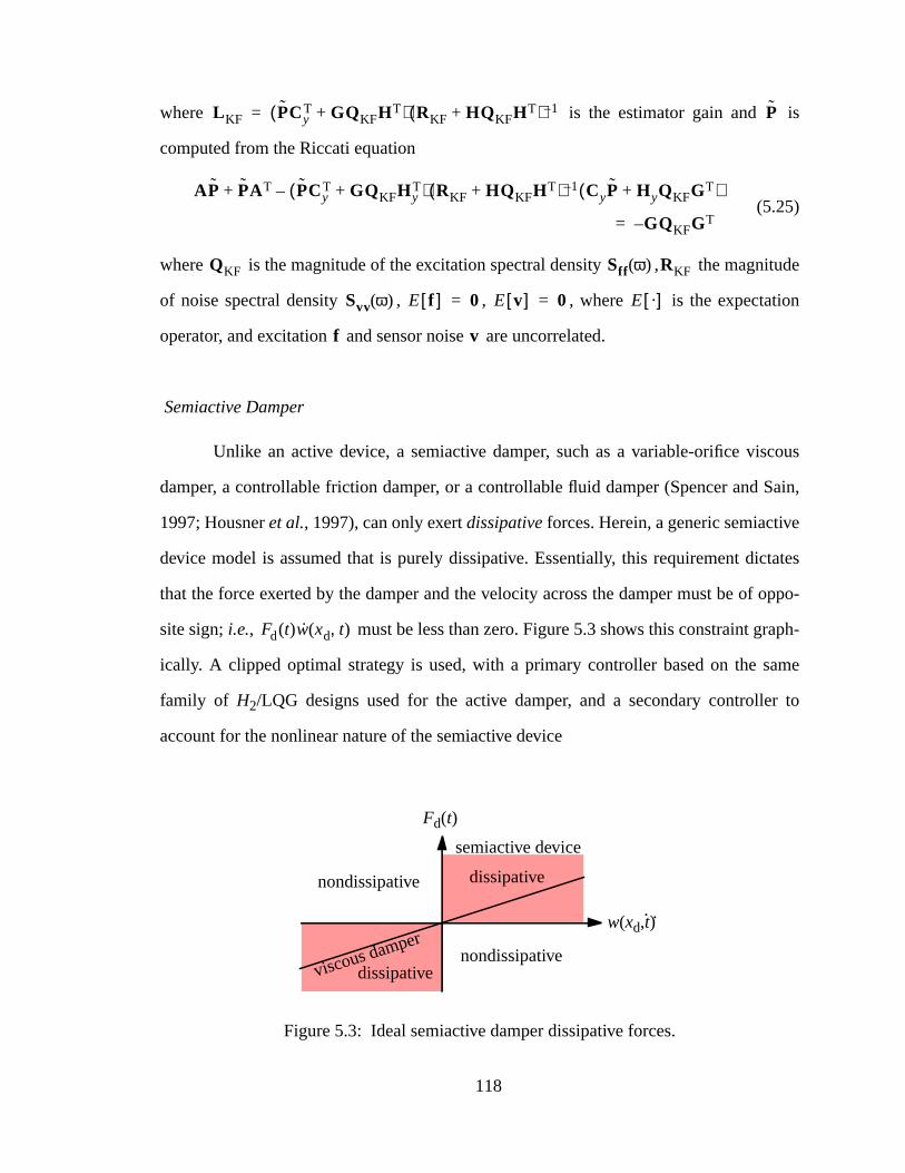
s
tude
on
cous
Sain,
e
tates
oppo-
ph-
ame
r to
where is the estimator gain and i
computed from the Riccati equation
(5.25)
where is the magnitude of the excitation spectral density , the magni
of noise spectral density , , , where is the expectati
operator, and excitation and sensor noise are uncorrelated.
Semiactive Damper
Unlike an active device, a semiactive damper, such as a variable-orifice vis
damper, a controllable friction damper, or a controllable fluid damper (Spencer and
1997; Housneret al., 1997), can only exertdissipativeforces. Herein, a generic semiactiv
device model is assumed that is purely dissipative. Essentially, this requirement dic
that the force exerted by the damper and the velocity across the damper must be of
site sign;i.e., must be less than zero. Figure 5.3 shows this constraint gra
ically. A clipped optimal strategy is used, with a primary controller based on the s
family of H2/LQG designs used for the active damper, and a secondary controlle
account for the nonlinear nature of the semiactive device
L KF PCyT GQKFHT+( ) RKF HQKFHT+( ) 1–= P
AP PAT PCyT GQKFHy
T+( ) RKF HQKFHT+( ) 1– CyP HyQKFGT+( )–+
GQKFGT–=
QKF Sff ω( ) RKF
Svv ω( ) E f[ ] 0= E v[ ] 0= E ·[ ]
f v
Fd t( )w xd t,( )
Fd(t)
w(xd,t).
Figure 5.3: Ideal semiactive damper dissipative forces.
viscous damper
semiactive device
.
dissipative
nondissipative
nondissipative
dissipative
118
ple-
ctive
is an
amper
pable
plot
this,
ance
the
cribed
func-
of the
with a
iactive
le sys-
(5.26)
Here, the secondary controller simply clips non-dissipative commands. For im
mentation, a bang-bang controller with force feedback has been shown to be effe
(Dykeet al., 1996a).
The semiactive device introduced here and used for the analysis in Chapter 6
ideal semiactive device. Of course actual semiactive devices, such as the smart d
examined in Chapters 7 and 8, may be limited in its performance and may not be ca
of achieving all forces in the first and third quadrants of the force versus velocity
shown in Figure 5.3. This limit is identified and discussed in Chapter 8. Having noted
the ideal semiactive device does, however, provide an “upper bound” on the perform
one could expect from a semiactive device.
5.4 Chapter Summary
The effects of cable sag, inclination, and axial stiffness are introduced into
dynamic model of transverse in-plane cable vibration. These parameters are des
completely by the independent parameter . The Galerkin approach using 20 sine
tions and a static deflection shape are used to accurately provide a low-order model
cable system. The static deflection shape used is the static profile of a flat-sag cable
point load applied to the cable at the location of the damper. Passive, active and sem
control strategies are presented. The effects of the sag on the performance of the cab
tem are examined in Chapter 6 using the cable model defined here.
Fd t( )Fd
active t( ) Fdactive t( )v xd t,( ) 0<
0 otherwise
=
λ2
119
ular
med to
n the
via a
emi-
lled as
orth
is, by
will
e and
, the
per-
able/
cation
iffer-
lines
amp-
CHAPTER 6: CABLE DAMPING CONTROL: EFFECTS OF CABLE SAG
In this chapter, the effect of cable sag on cable damping control, in partic
damping ratio, cable response, and damper location, is examined. The cable is assu
have virtually no inherent damping without the supplemental damper, about 0.005% i
first mode. Root mean square (RMS) responses to the excitation are computed
Lyapunov solution for linear (passive and active) strategies and from simulation for s
active dampers. A 1% RMS sensor noise corrupts each sensor measurement (mode
Gaussian pulse processes).
6.1 Effects of Sag on Damping Ratio
Before examining RMS responses with passive and semiactive dampers, it is w
studying the modal properties of the controlled system. Since the semiactive system
definition nonlinear, the active system will be used to compute modal properties and
be compared with passive modal damping. The RMS responses of the optimal activ
optimal semiactive damping strategies will be seen below to be quite similar. Thus
modal properties of the active system are a good indication of “equivalent” modal pro
ties for the semiactive system.
The modal damping that can be provided to the fundamental mode of the c
damper system by passive and active dampers is shown in Figure 6.1 for a damper lo
xd = 0.02. (The reader may note that the five markers, whether filled or not, denote d
ent levels ofλ2, whereas dashed lines with open markers denote the passive, and solid
with filled markers denote the active results.) In the absence of sag, the maximum d
120
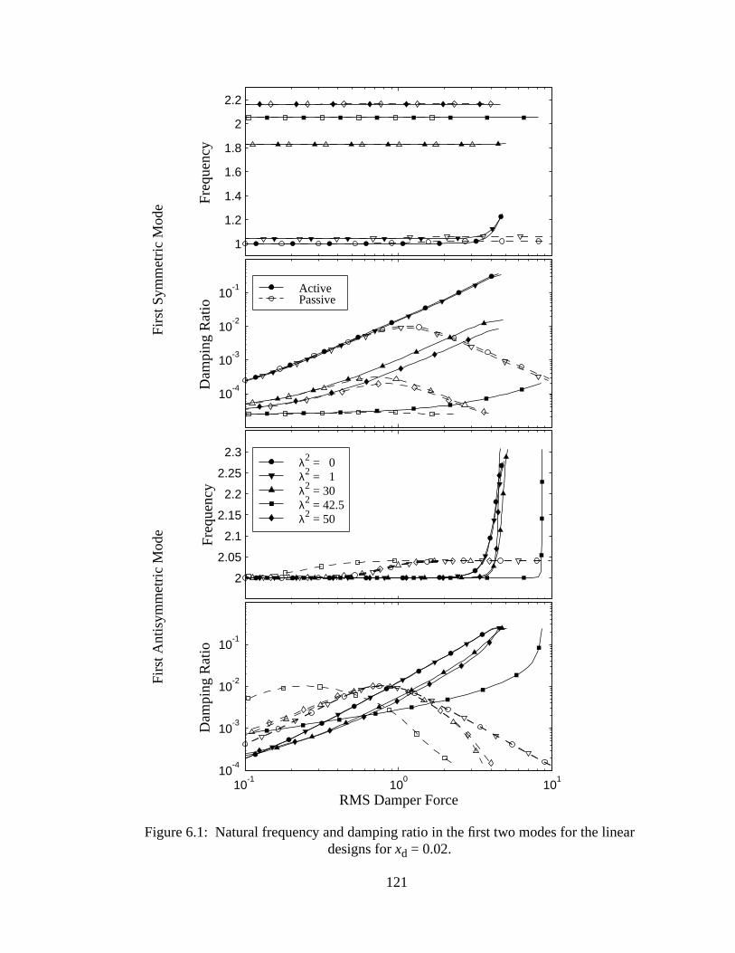
ar
1
1.2
1.4
1.6
1.8
2
2.2
Freq
uenc
y
10-4
10-3
10-2
10-1
Dam
ping
Rat
io
ActivePassive
2
2.05
2.1
2.15
2.2
2.25
2.3
Freq
uenc
y
λ2 = 0λ2 = 1λ2 = 30λ2 = 42.5λ2 = 50
10-1
100
101
10-4
10-3
10-2
10-1
RMS Damper Force
Dam
ping
Rat
io
Figure 6.1: Natural frequency and damping ratio in the first two modes for the linedesigns forxd = 0.02.
Firs
t Sym
met
ric M
ode
Firs
t Ant
isym
met
ric M
ode
121
active
% (a
ng
ever,
. For
only
uced,
-
met-
es to
ments
e and
er the
of
ive
dies
tive
cept
g.
the
ill be
. Fig-
con-
ing in the first symmetric mode provided by a passive damper is 1.03%, whereas the
damper provides over 36% of critical damping. With small sag,λ2 = 1, the passive damp-
ing is degraded slightly to 0.91% (a factor of 0.88); the active system drops to 33.6
factor of 0.93). For a larger sagλ2 = 30, the passive damper is less effective, providi
only 0.04% damping (a factor of 0.039 compared to no sag). The active device, how
still provides almost a 1.6% damping ratio (a factor of 0.044 compared to no sag)
λ2 = 42.5, the passive damper is ineffective for the first symmetric mode, providing
0.002% damping. The active device for this particular level of sag is also severely red
providing only 0.04% damping. For yet larger sag atλ2 = 50, a passive damper can pro
vide 0.04% damping and the active strategy can provide 1% damping in the first sym
ric mode. The natural frequency of the first symmetric mode for larger sag increas
over twice the value at small sag, which gives the cable somewhat smaller displace
with the same excitation, but does not degrade the improvements seen with activ
(below) semiactive dampers. The natural frequencies remain relatively constant ov
range ofxd.
Sag has virtually no effect, except for sag levels in the immediate vicinity
λ2 = 39.5 and 41.93 (note thatλ2 = 42.5 even appears unaffected by sag), on pass
damping for the first antisymmetric mode; this result is consistent with previous stu
(Sulekh, 1990), with the damping remaining about 1% of critical. Similarly, the ac
control of the first antisymmetric mode is unaffected by the inclusion of sag, again ex
for sag levels in the immediate vicinity ofλ2 = 39.5 and 41.93, achieving 30% dampin
The significance ofλ2 = 39.5 and 41.93 are identified in the subsequent discussion on
effects of sag and inclination on modal characteristics of the controlled system, and w
explained in a discussion of the effects of sag on RMS cable response in Section 6.2
ure 6.1 does indicate that an optimal level of control does exists for both the passive
trol and for the active control strategy.
122
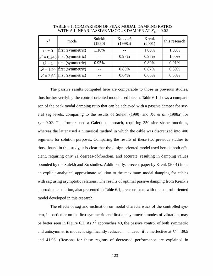
udies,
pari-
r sev-
tions,
o 400
ies to
effi-
alues
finds
bles
nk’s
ented
sys-
ay
tric
ed in
The passive results computed here are comparable to those in previous st
thus further verifying the control-oriented model used herein. Table 6.1 shows a com
son of the peak modal damping ratio that can be achieved with a passive damper fo
eral sag levels, comparing to the results of Sulekh (1990) and Xuet al. (1998a) for
xd = 0.02. The former used a Galerkin approach, requiring 350 sine shape func
whereas the latter used a numerical method in which the cable was discretized int
segments for solution purposes. Comparing the results of these two previous stud
those found in this study, it is clear that the design oriented model used here is both
cient, requiring only 21 degrees-of-freedom, and accurate, resulting in damping v
bounded by the Sulekh and Xu studies. Additionally, a recent paper by Krenk (2001)
an explicit analytical approximate solution to the maximum modal damping for ca
with sag using asymptotic relations. The results of optimal passive damping from Kre
approximate solution, also presented in Table 6.1, are consistent with the control ori
model developed in this research.
The effects of sag and inclination on modal characteristics of the controlled
tem, in particular on the first symmetric and first antisymmetric modes of vibration, m
be better seen in Figure 6.2. Asλ2 approaches 40, the passive control of both symme
and antisymmetric modes is significantly reduced — indeed, it is ineffective atλ2 = 39.5
and 41.93. (Reasons for these regions of decreased performance are explain
TABLE 6.1: COMPARISON OF PEAK MODAL DAMPING RATIOSWITH A LINEAR PASSIVE VISCOUS DAMPER ATXD = 0.02
λ2 modeSulekh(1990)
Xu et al.(1998a)
Krenk(2001)
this research
λ2 = 0 first (symmetric) 1.10% -- 1.00% 1.03%
λ2 = 0.245first (symmetric) -- 0.98% 0.97% 1.00%
λ2 = 1 first (symmetric) 0.95% -- 0.89% 0.91%
λ2 = 1.20 first (symmetric) -- 0.85% 0.87% 0.89%
λ2 = 3.63 first (symmetric) -- 0.64% 0.66% 0.68%
123
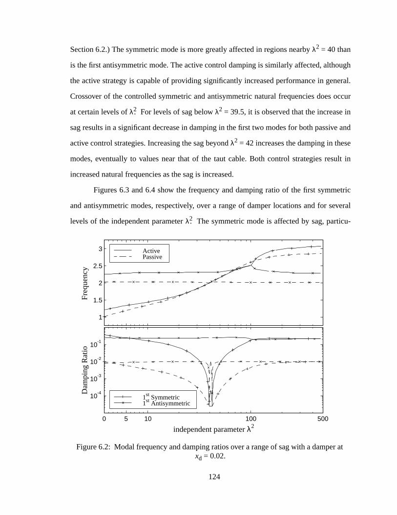
ugh
eral.
occur
in
e and
e
ult in
etric
everal
u-
r at
Section 6.2.) The symmetric mode is more greatly affected in regions nearbyλ2 = 40 than
is the first antisymmetric mode. The active control damping is similarly affected, altho
the active strategy is capable of providing significantly increased performance in gen
Crossover of the controlled symmetric and antisymmetric natural frequencies does
at certain levels ofλ2. For levels of sag belowλ2 = 39.5, it is observed that the increase
sag results in a significant decrease in damping in the first two modes for both passiv
active control strategies. Increasing the sag beyondλ2 = 42 increases the damping in thes
modes, eventually to values near that of the taut cable. Both control strategies res
increased natural frequencies as the sag is increased.
Figures 6.3 and 6.4 show the frequency and damping ratio of the first symm
and antisymmetric modes, respectively, over a range of damper locations and for s
levels of the independent parameterλ2. The symmetric mode is affected by sag, partic
1
1.5
2
2.5
3
Freq
uenc
y
ActivePassive
0 5 10 100 500
10-4
10-3
10-2
10-1
Dam
ping
Rat
io
independent parameter λ2
1st Symmetric1st Antisymmetric
Figure 6.2: Modal frequency and damping ratios over a range of sag with a dampexd = 0.02.
124
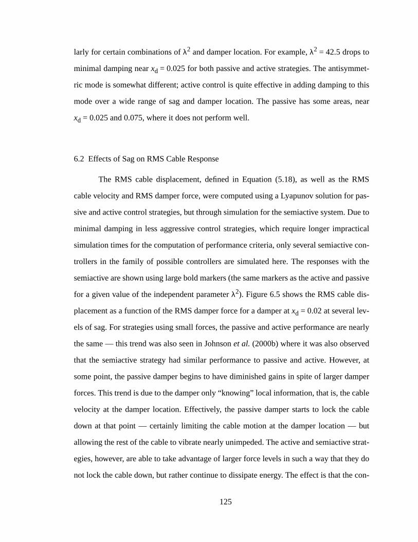
et-
this
s, near
MS
pas-
ue to
tical
con-
the
passive
-
nearly
d
er, at
amper
ble
able
but
strat-
ey do
con-
larly for certain combinations ofλ2 and damper location. For example,λ2 = 42.5 drops to
minimal damping nearxd = 0.025 for both passive and active strategies. The antisymm
ric mode is somewhat different; active control is quite effective in adding damping to
mode over a wide range of sag and damper location. The passive has some area
xd = 0.025 and 0.075, where it does not perform well.
6.2 Effects of Sag on RMS Cable Response
The RMS cable displacement, defined in Equation (5.18), as well as the R
cable velocity and RMS damper force, were computed using a Lyapunov solution for
sive and active control strategies, but through simulation for the semiactive system. D
minimal damping in less aggressive control strategies, which require longer imprac
simulation times for the computation of performance criteria, only several semiactive
trollers in the family of possible controllers are simulated here. The responses with
semiactive are shown using large bold markers (the same markers as the active and
for a given value of the independent parameterλ2). Figure 6.5 shows the RMS cable dis
placement as a function of the RMS damper force for a damper atxd = 0.02 at several lev-
els of sag. For strategies using small forces, the passive and active performance are
the same — this trend was also seen in Johnsonet al. (2000b) where it was also observe
that the semiactive strategy had similar performance to passive and active. Howev
some point, the passive damper begins to have diminished gains in spite of larger d
forces. This trend is due to the damper only “knowing” local information, that is, the ca
velocity at the damper location. Effectively, the passive damper starts to lock the c
down at that point — certainly limiting the cable motion at the damper location —
allowing the rest of the cable to vibrate nearly unimpeded. The active and semiactive
egies, however, are able to take advantage of larger force levels in such a way that th
not lock the cable down, but rather continue to dissipate energy. The effect is that the
125
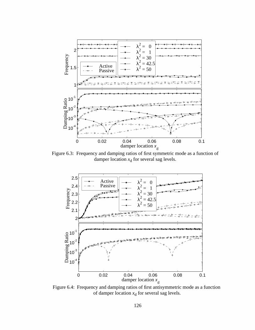
of
on
2
2.1
2.2
2.3
2.4
2.5
Freq
uenc
y
ActivePassive
0 0.02 0.04 0.06 0.08 0.1
10-4
10-3
10-2
10-1
Dam
ping
Rat
io
damper location xd
λ2 = 0λ2 = 1λ2 = 30λ2 = 42.5λ2 = 50
1
1.5
2
Freq
uenc
yActivePassive
0 0.02 0.04 0.06 0.08 0.1
10-4
10-3
10-2
10-1
Dam
ping
Rat
io
damper location xd
λ2 = 0λ2 = 1λ2 = 30λ2 = 42.5λ2 = 50
Figure 6.3: Frequency and damping ratios of first symmetric mode as a function damper locationxd for several sag levels.
Figure 6.4: Frequency and damping ratios of first antisymmetric mode as a functiof damper locationxd for several sag levels.
126
ction,
cous
ameter
nse
d, the
di-
ed in
sponse
7 pro-
g of
in the
le
us, it
for a
orces,
f
trollable semiactive damper is able to achieve a 50% to 80% displacement redu
depending on the sag, compared to the optimal passive linear viscous damper.
Figure 6.6 shows the RMS cable displacement for the passive linear vis
damper, and the optimal active and semiactive dampers versus the independent par
λ2. Without sag (λ2 = 0), the semiactive damper can provide about a 71% respo
decrease compared to the best passive device. With small sag (λ2 = 1), the RMS displace-
ments decrease little for all three damping strategies. Forλ2 = 30, the control performance
for passive, active, and semiactive strategies begin to degrade and aroundλ2 = 40, the
same region where the damping in the first two modes was significantly decrease
RMS performance is poor. Increasingλ2, the performance improves, but there are ad
tional regions where all methods are ineffective. This phenomenon will be discuss
detail in the next section. Nevertheless, the semiactive damper always decreases re
compared to the best passive damper, by as much as 60% to 80%.
To observe what happens near the peaks of reduced performance, Figure 6.
vides a closer look. Indeed, the region of decreased performance aroundλ2 = 40 consists
of two peaks of poor performance with a valley of better performance. The pairin
these two peaks is found for each of the three regions of decreased performance
[0,500] range ofλ2 values studied here. The peaks of poor performance occur atλ2 values
of 4π2, 41.93, 16π2, 167.79, 36π2 and 377.59. Similar results are seen in RMS cab
velocity in Figure 6.8 (though there is a small increase from no sag to small sag). Th
may be concluded that a “smart” damper may provide superior damping to cables
large range of cable sag. Note, however, that the benefit comes with larger damper f
though these force levels (Johnsonet al., 2000b) are still well within the capabilities o
current damper technology.
127
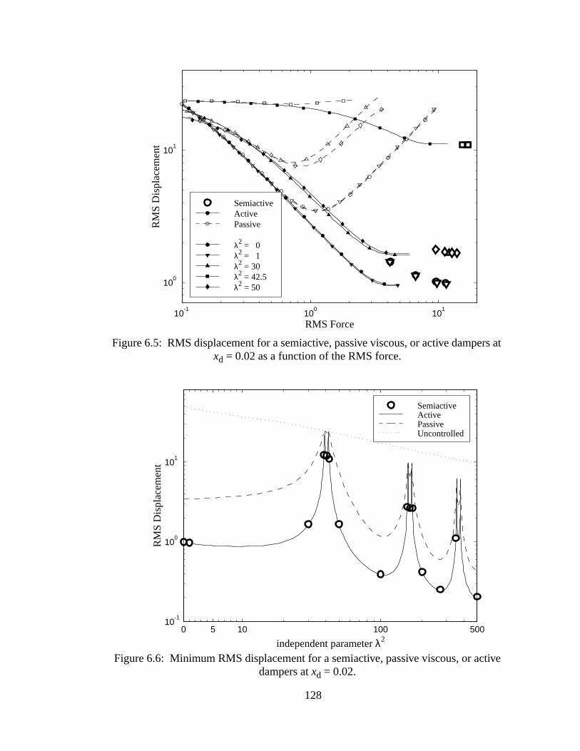
s at
ive
0 5 10 100 50010
-1
100
101
RM
S D
ispl
acem
ent
independent parameter λ2
SemiactiveActivePassiveUncontrolled
10-1
100
101
100
101
RM
S D
ispl
acem
ent
RMS Force
SemiactiveActivePassive
λ2 = 0λ2 = 1λ2 = 30λ2 = 42.5λ2 = 50
Figure 6.5: RMS displacement for a semiactive, passive viscous, or active damperxd = 0.02 as a function of the RMS force.
Figure 6.6: Minimum RMS displacement for a semiactive, passive viscous, or actdampers atxd = 0.02.
128
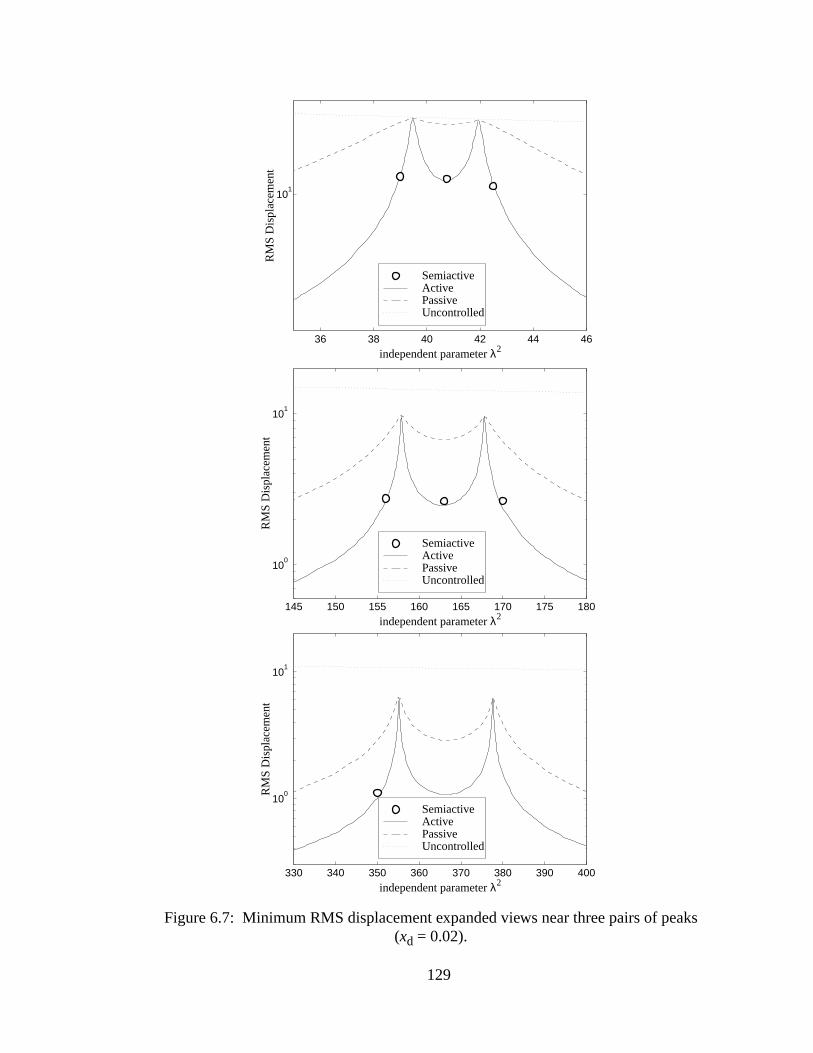
ks
330 340 350 360 370 380 390 400
100
101
RM
S D
ispl
acem
ent
independent parameter λ2
SemiactiveActivePassiveUncontrolled
145 150 155 160 165 170 175 180
100
101
RM
S D
ispl
acem
ent
independent parameter λ2
SemiactiveActivePassiveUncontrolled
36 38 40 42 44 46
101
RM
S D
ispl
acem
ent
independent parameter λ2
SemiactiveActivePassiveUncontrolled
Figure 6.7: Minimum RMS displacement expanded views near three pairs of pea(xd = 0.02).
129
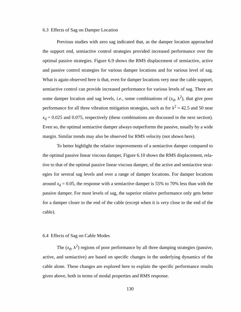
ached
er the
active
f sag.
pport,
re are
ction).
wide
d to
t, rela-
strat-
ations
h the
better
sive,
of the
results
6.3 Effects of Sag on Damper Location
Previous studies with zero sag indicated that, as the damper location appro
the support end, semiactive control strategies provided increased performance ov
optimal passive strategies. Figure 6.9 shows the RMS displacement of semiactive,
and passive control strategies for various damper locations and for various level o
What is again observed here is that, even for damper locations very near the cable su
semiactive control can provide increased performance for various levels of sag. The
some damper location and sag levels,i.e., some combinations of (xd, λ2), that give poor
performance for all three vibration mitigation strategies, such as forλ2 = 42.5 and 50 near
xd = 0.025 and 0.075, respectively (these combinations are discussed in the next se
Even so, the optimal semiactive damper always outperforms the passive, usually by a
margin. Similar trends may also be observed for RMS velocity (not shown here).
To better highlight the relative improvements of a semiactive damper compare
the optimal passive linear viscous damper, Figure 6.10 shows the RMS displacemen
tive to that of the optimal passive linear viscous damper, of the active and semiactive
egies for several sag levels and over a range of damper locations. For damper loc
aroundxd = 0.05, the response with a semiactive damper is 55% to 70% less than wit
passive damper. For most levels of sag, the superior relative performance only gets
for a damper closer to the end of the cable (except when it isveryclose to the end of the
cable).
6.4 Effects of Sag on Cable Modes
The (xd, λ2) regions of poor performance by all three damping strategies (pas
active, and semiactive) are based on specific changes in the underlying dynamics
cable alone. These changes are explored here to explain the specific performance
given above, both in terms of modal properties and RMS response.
130
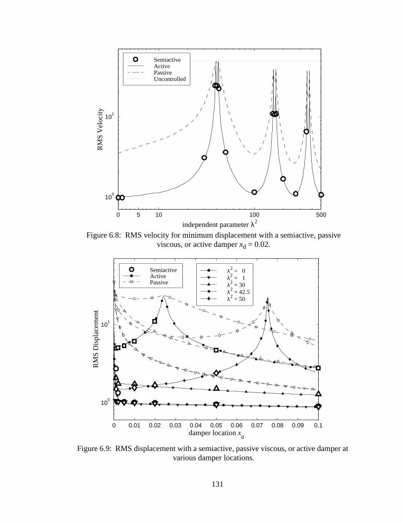
r at
0 0.01 0.02 0.03 0.04 0.05 0.06 0.07 0.08 0.09 0.1
100
101
RM
S D
ispl
acem
ent
damper location xd
λ2 = 0λ2 = 1λ2 = 30λ2 = 42.5λ2 = 50
SemiactiveActivePassive
Figure 6.9: RMS displacement with a semiactive, passive viscous, or active dampevarious damper locations.
0 5 10 100 500
100
101
RM
S V
eloc
ity
independent parameter λ2
SemiactiveActivePassiveUncontrolled
Figure 6.8: RMS velocity for minimum displacement with a semiactive, passiveviscous, or active damperxd = 0.02.
131
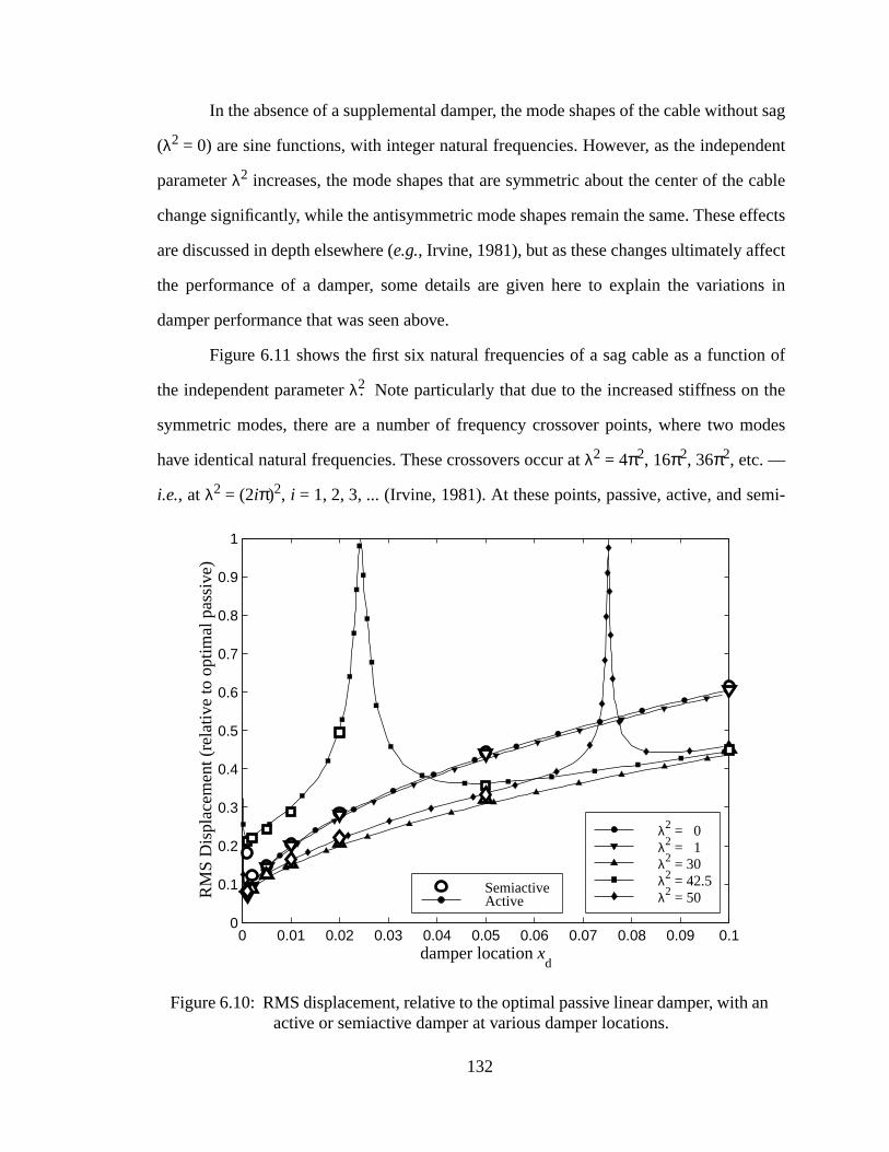
ut sag
ndent
cable
effects
ct
ns in
on of
the
odes
mi-
an
In the absence of a supplemental damper, the mode shapes of the cable witho
(λ2 = 0) are sine functions, with integer natural frequencies. However, as the indepe
parameterλ2 increases, the mode shapes that are symmetric about the center of the
change significantly, while the antisymmetric mode shapes remain the same. These
are discussed in depth elsewhere (e.g., Irvine, 1981), but as these changes ultimately affe
the performance of a damper, some details are given here to explain the variatio
damper performance that was seen above.
Figure 6.11 shows the first six natural frequencies of a sag cable as a functi
the independent parameterλ2. Note particularly that due to the increased stiffness on
symmetric modes, there are a number of frequency crossover points, where two m
have identical natural frequencies. These crossovers occur atλ2 = 4π2, 16π2, 36π2, etc. —
i.e., at λ2 = (2iπ)2, i = 1, 2, 3, ... (Irvine, 1981). At these points, passive, active, and se
0 0.01 0.02 0.03 0.04 0.05 0.06 0.07 0.08 0.09 0.10
0.1
0.2
0.3
0.4
0.5
0.6
0.7
0.8
0.9
1
RM
S D
ispl
acem
ent (
rela
tive
to o
ptim
al p
assi
ve)
damper location xd
λ2 = 0λ2 = 1λ2 = 30λ2 = 42.5λ2 = 50
SemiactiveActive
Figure 6.10: RMS displacement, relative to the optimal passive linear damper, withactive or semiactive damper at various damper locations.
132
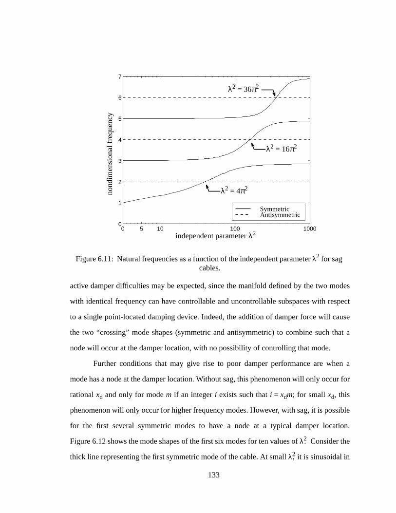
odes
spect
ause
hat a
en a
ur for
sible
tion.
active damper difficulties may be expected, since the manifold defined by the two m
with identical frequency can have controllable and uncontrollable subspaces with re
to a single point-located damping device. Indeed, the addition of damper force will c
the two “crossing” mode shapes (symmetric and antisymmetric) to combine such t
node will occur at the damper location, with no possibility of controlling that mode.
Further conditions that may give rise to poor damper performance are wh
mode has a node at the damper location. Without sag, this phenomenon will only occ
rationalxd and only for modem if an integeri exists such thati = xdm; for small xd, this
phenomenon will only occur for higher frequency modes. However, with sag, it is pos
for the first several symmetric modes to have a node at a typical damper loca
Figure 6.12 shows the mode shapes of the first six modes for ten values ofλ2. Consider the
thick line representing the first symmetric mode of the cable. At smallλ2, it is sinusoidal in
0 5 10 100 10000
1
2
3
4
5
6
7
SymmetricAntisymmetric
Figure 6.11: Natural frequencies as a function of the independent parameterλ2 for sagcables.
independent parameterλ2
nond
imen
sion
al fr
eque
ncy
λ2 = 4π2
λ2 = 16π2
λ2 = 36π2
133
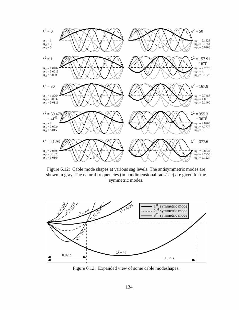
arehe
λ2 = 0
λ2 = 1
λ2 = 30
λ2 = 39.478
λ2 = 41.93
= 4π2
λ2 = 50
λ2 = 157.91
λ2 = 167.8
λ2 = 355.3
λ2 = 377.6
= 36π2
= 16π2
ωs1 = 1ωs2 = 3ωs3 = 5
ωs1 = 1.0402ωs2 = 3.0015ωs3 = 5.0003
ωs1 = 1.8264ωs2 = 3.0632ωs3 = 5.0111
ωs1 = 2ωs2 = 3.0934ωs3 = 5.0153
ωs1 = 2.0406ωs2 = 3.1023ωs3 = 5.0164
ωs1 = 2.1626ωs2 = 3.1354ωs3 = 5.0203
ωs1 = 2.7375ωs2 = 4ωs3 = 5.1222
ωs1 = 2.7486ωs2 = 4.0816ωs3 = 5.1400
ωs1 = 2.8205ωs2 = 4.7777ωs3 = 6
ωs1 = 2.8234ωs2 = 4.7955ωs3 = 6.1224
Figure 6.12: Cable mode shapes at various sag levels. The antisymmetric modesshown in gray. The natural frequencies (in nondimensional rads/sec) are given for t
symmetric modes.
λ2 =
41.93
λ2 = 50
λ2 =
16π2
λ2 =
36π2
λ2 =
167
.8
λ2 = 4π2
λ2 =
377.
6
Figure 6.13: Expanded view of some cable modeshapes.
0.02L0.075L
1st
2nd
3rdsymmetric modesymmetric mode
symmetric mode
134
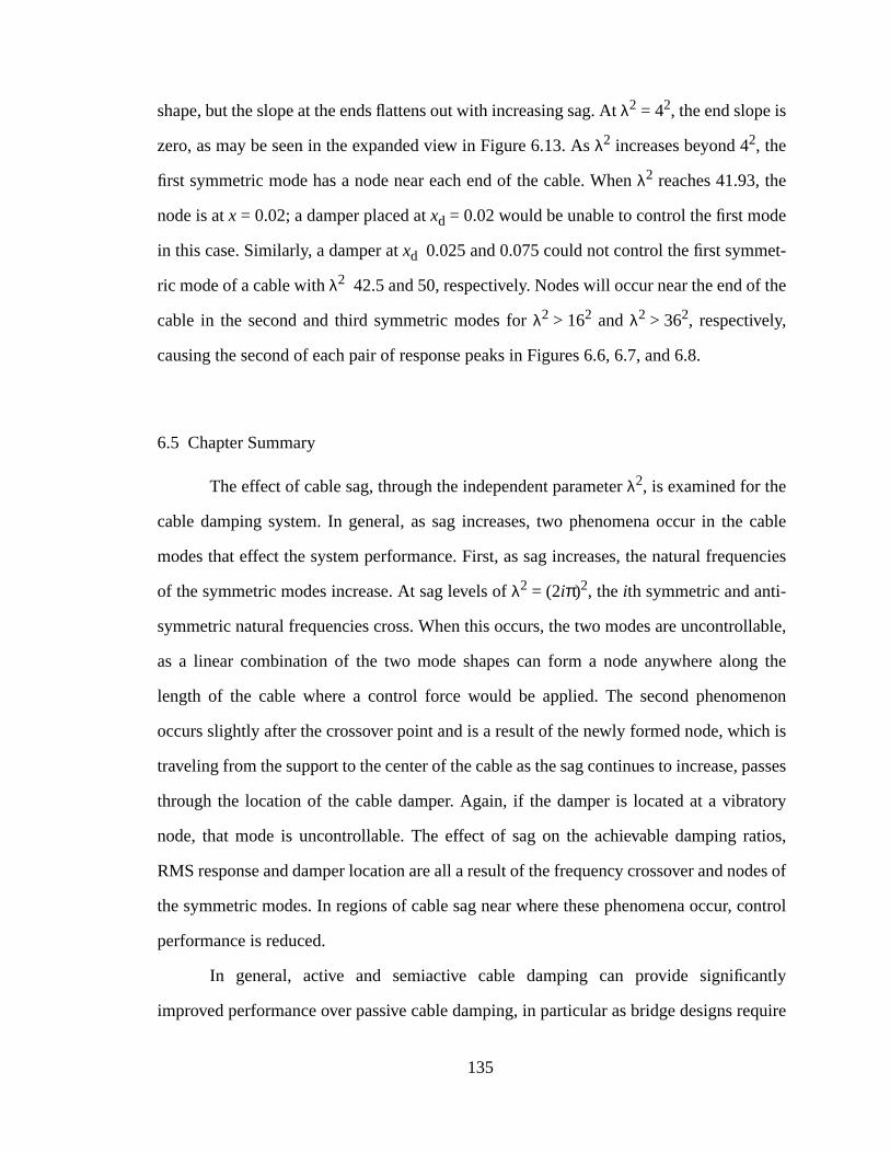
e
t-
the
cable
encies
llable,
g the
enon
ch is
passes
tory
atios,
des of
control
ntly
equire
shape, but the slope at the ends flattens out with increasing sag. Atλ2 = 42, the end slope is
zero, as may be seen in the expanded view in Figure 6.13. Asλ2 increases beyond 42, the
first symmetric mode has a node near each end of the cable. Whenλ2 reaches 41.93, the
node is atx = 0.02; a damper placed atxd = 0.02 would be unable to control the first mod
in this case. Similarly, a damper atxd 0.025 and 0.075 could not control the first symme
ric mode of a cable withλ2 42.5 and 50, respectively. Nodes will occur near the end of
cable in the second and third symmetric modes forλ2 > 162 and λ2 > 362, respectively,
causing the second of each pair of response peaks in Figures 6.6, 6.7, and 6.8.
6.5 Chapter Summary
The effect of cable sag, through the independent parameterλ2, is examined for the
cable damping system. In general, as sag increases, two phenomena occur in the
modes that effect the system performance. First, as sag increases, the natural frequ
of the symmetric modes increase. At sag levels ofλ2 = (2iπ)2, the ith symmetric and anti-
symmetric natural frequencies cross. When this occurs, the two modes are uncontro
as a linear combination of the two mode shapes can form a node anywhere alon
length of the cable where a control force would be applied. The second phenom
occurs slightly after the crossover point and is a result of the newly formed node, whi
traveling from the support to the center of the cable as the sag continues to increase,
through the location of the cable damper. Again, if the damper is located at a vibra
node, that mode is uncontrollable. The effect of sag on the achievable damping r
RMS response and damper location are all a result of the frequency crossover and no
the symmetric modes. In regions of cable sag near where these phenomena occur,
performance is reduced.
In general, active and semiactive cable damping can provide significa
improved performance over passive cable damping, in particular as bridge designs r
135

How-
ideal
rfor-
. For
e con-
ctive
longer cables and the damper location, relative to the length of the cable, is reduced.
ever, the research indicating this increased performance in this chapter assumes
active and semiactive control devices. For the semiactive control to achieve similar pe
mance to active control, the semiactive device must exhibit excellent performance
less than perfect semiactive damper performance, the performance of the semiactiv
trol strategy will be effected. The next chapter, Chapter 7, considers a realistic semia
smart fluid damper for experimental verification of semiactive cable damping.
136
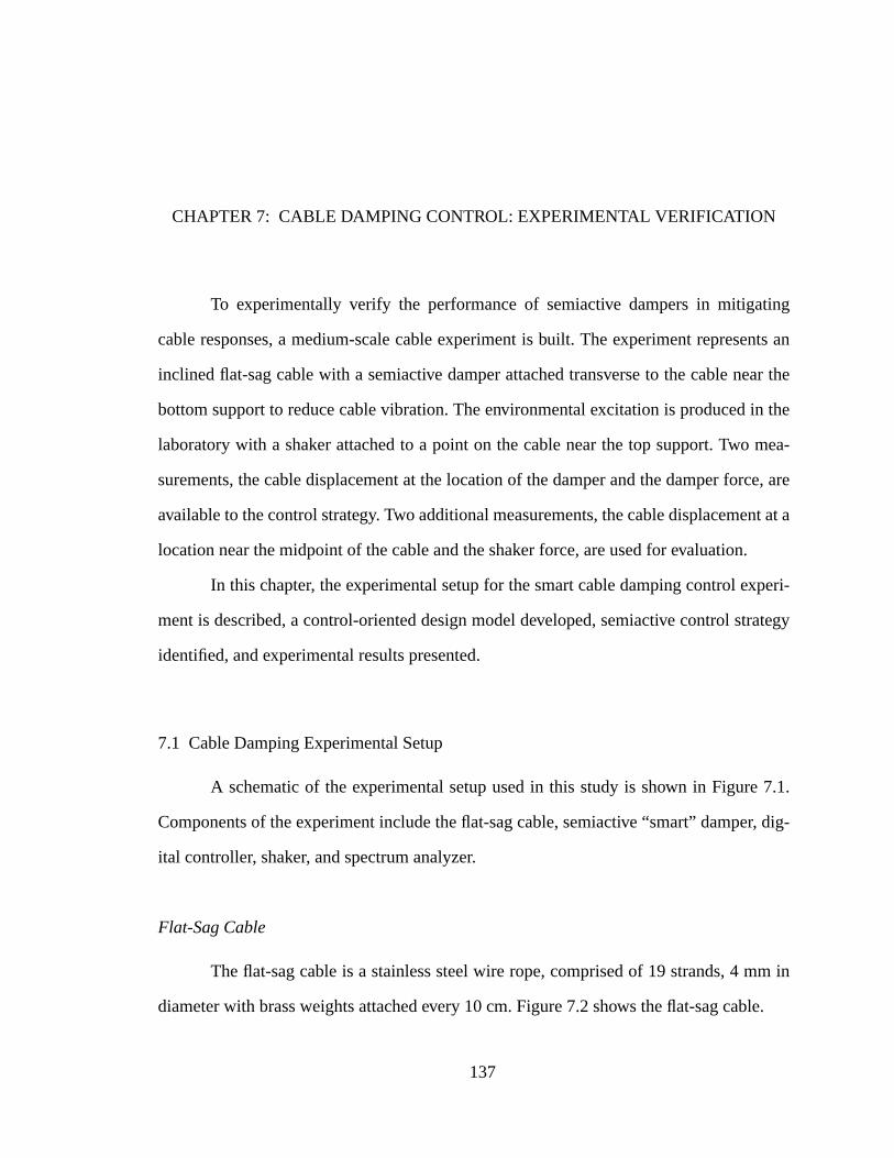
ing
nts an
ar the
n the
mea-
ce, are
nt at a
.
peri-
rategy
7.1.
r, dig-
m in
ble.
CHAPTER 7: CABLE DAMPING CONTROL: EXPERIMENTAL VERIFICATION
To experimentally verify the performance of semiactive dampers in mitigat
cable responses, a medium-scale cable experiment is built. The experiment represe
inclined flat-sag cable with a semiactive damper attached transverse to the cable ne
bottom support to reduce cable vibration. The environmental excitation is produced i
laboratory with a shaker attached to a point on the cable near the top support. Two
surements, the cable displacement at the location of the damper and the damper for
available to the control strategy. Two additional measurements, the cable displaceme
location near the midpoint of the cable and the shaker force, are used for evaluation
In this chapter, the experimental setup for the smart cable damping control ex
ment is described, a control-oriented design model developed, semiactive control st
identified, and experimental results presented.
7.1 Cable Damping Experimental Setup
A schematic of the experimental setup used in this study is shown in Figure
Components of the experiment include the flat-sag cable, semiactive “smart” dampe
ital controller, shaker, and spectrum analyzer.
Flat-Sag Cable
The flat-sag cable is a stainless steel wire rope, comprised of 19 strands, 4 m
diameter with brass weights attached every 10 cm. Figure 7.2 shows the flat-sag ca
137
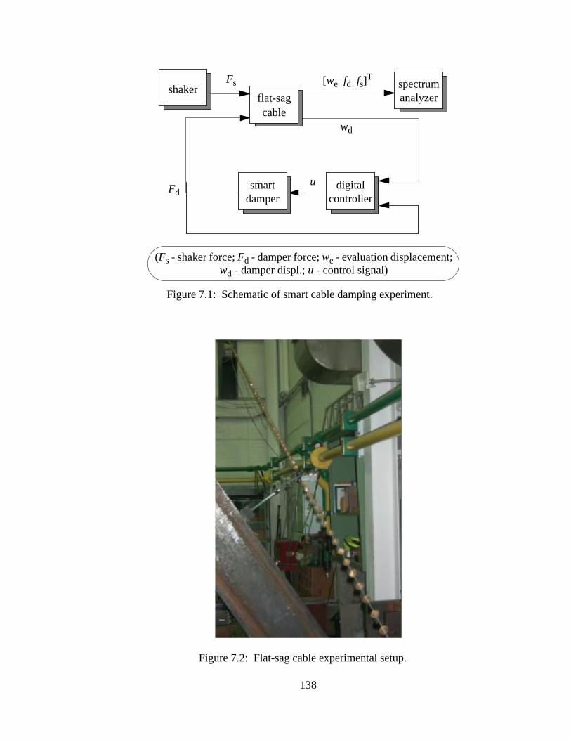
Figure 7.1: Schematic of smart cable damping experiment.
shakerflat-sagcable
spectrumanalyzer
Fs [we fd fs]T
wd
Fdusmart
damperdigital
controller
(Fs - shaker force;Fd - damper force;we - evaluation displacement;wd - damper displ.;u - control signal)
Figure 7.2: Flat-sag cable experimental setup.
138
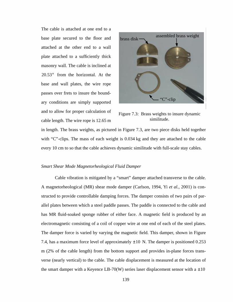
ether
able
les.
able.
f par-
ble and
y an
lates.
gure
.253
ans-
tion of
The cable is attached at one end to a
base plate secured to the floor and
attached at the other end to a wall
plate attached to a sufficiently thick
masonry wall. The cable is inclined at
from the horizontal. At the
base and wall plates, the wire rope
passes over frets to insure the bound-
ary conditions are simply supported
and to allow for proper calculation of
cable length. The wire rope is 12.65 m
in length. The brass weights, as pictured in Figure 7.3, are two piece disks held tog
with “C”-clips. The mass of each weight is 0.034 kg and they are attached to the c
every 10 cm to so that the cable achieves dynamic similitude with full-scale stay cab
Smart Shear Mode Magnetorheological Fluid Damper
Cable vibration is mitigated by a “smart” damper attached transverse to the c
A magnetorheological (MR) shear mode damper (Carlson, 1994, Yiet al., 2001) is con-
structed to provide controllable damping forces. The damper consists of two pairs o
allel plates between which a steel paddle passes. The paddle is connected to the ca
has MR fluid-soaked sponge rubber of either face. A magnetic field is produced b
electromagnetic consisting of a coil of copper wire at one end of each of the steel p
The damper force is varied by varying the magnetic field. This damper, shown in Fi
7.4, has a maximum force level of approximately N. The damper is positioned 0
m (2% of the cable length) from the bottom support and provides in-plane forces tr
verse (nearly vertical) to the cable. The cable displacement is measured at the loca
the smart damper with a Keyence LB-70(W) series laser displacement sensor with a
Figure 7.3: Brass weights to insure dynamicsimilitude.
brass disk
“C”-clip
assembled brass weight
20.53°
10±
10±
139
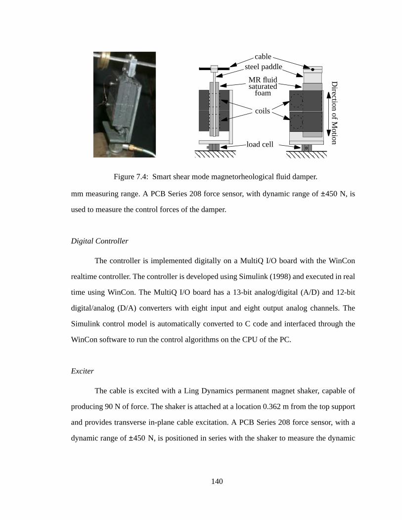
N, is
n
real
bit
The
the
le of
pport
with a
amic
mm measuring range. A PCB Series 208 force sensor, with dynamic range of
used to measure the control forces of the damper.
Digital Controller
The controller is implemented digitally on a MultiQ I/O board with the WinCo
realtime controller. The controller is developed using Simulink (1998) and executed in
time using WinCon. The MultiQ I/O board has a 13-bit analog/digital (A/D) and 12-
digital/analog (D/A) converters with eight input and eight output analog channels.
Simulink control model is automatically converted to C code and interfaced through
WinCon software to run the control algorithms on the CPU of the PC.
Exciter
The cable is excited with a Ling Dynamics permanent magnet shaker, capab
producing 90 N of force. The shaker is attached at a location 0.362 m from the top su
and provides transverse in-plane cable excitation. A PCB Series 208 force sensor,
dynamic range of N, is positioned in series with the shaker to measure the dyn
450±
Figure 7.4: Smart shear mode magnetorheological fluid damper.
MR fluidsaturated
foam
coils
cable
load cell
Direction of M
otionsteel paddle
450±
140
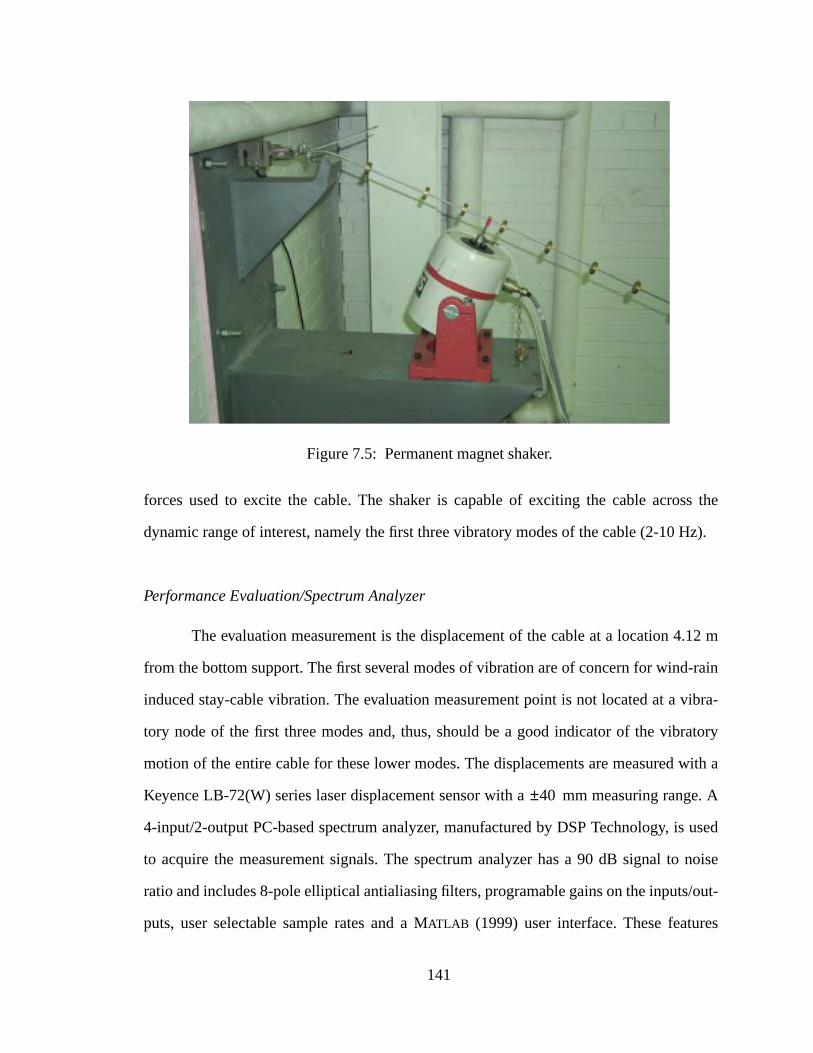
ss the
Hz).
.12 m
-rain
vibra-
atory
with a
ge. A
used
noise
/out-
s
forces used to excite the cable. The shaker is capable of exciting the cable acro
dynamic range of interest, namely the first three vibratory modes of the cable (2-10
Performance Evaluation/Spectrum Analyzer
The evaluation measurement is the displacement of the cable at a location 4
from the bottom support. The first several modes of vibration are of concern for wind
induced stay-cable vibration. The evaluation measurement point is not located at a
tory node of the first three modes and, thus, should be a good indicator of the vibr
motion of the entire cable for these lower modes. The displacements are measured
Keyence LB-72(W) series laser displacement sensor with a mm measuring ran
4-input/2-output PC-based spectrum analyzer, manufactured by DSP Technology, is
to acquire the measurement signals. The spectrum analyzer has a 90 dB signal to
ratio and includes 8-pole elliptical antialiasing filters, programable gains on the inputs
puts, user selectable sample rates and a MATLAB (1999) user interface. These feature
Figure 7.5: Permanent magnet shaker.
40±
141
tifi-
lity
alyti-
mode
iactive
eter
re are:
en-
er .
the
tatic
shape
allow for direct acquisition of high quality data and transfer functions for system iden
cation and response analysis.
7.2 System Identification of Cable Damping Model
A critical precursor to control design is development of a low order, high-qua
model of the system. In this section, the system input/output characteristics are an
cally derived by physically modeling the cable and damper. Flat-sag cable and shear
magnetorheological damper models are developed and combined to model the sem
cable damping system.
Flat-Sag Cable Model with Point Load Excitation
Using the flat-sag cable model identified previously, a model for the 12.65 m
cable, shown in Figure 7.6, is developed. The parameters for the cable tested he
kg/m, m, , N, N/m2,
m2, , , and
,and Hz.
The effects of cable sag, angle-of-inclination, and axial stiffness on the nondim
sional dynamic response of the system enter only though the independent paramet
For the experiment in this study, was determined to be . This value is within
[0,1] range typical for cable stayed-bridges. The sag ratio for this cable is 0.28%.
Using a Galerkin method, the transverse motion of the cable relative to the s
profile may be approximated with a finite series
(7.1)
where the shape functions, , include a sine series as well as static deflection
functions for the cable with sag introduced in Johnsonet al. (2001b) to account for the
ρ 0.407= L 12.65= θ 22.53°= H 2172= E 1.9 11×10=
A 1.26 5–×10= ζ1 0.0015= ζ2 0.003= ζ3 0.005=
ζi 1 2 3, ,≠ 0.0005= ω0 2.89=
λ2
λ2 0.59
w x t,( ) qj t( )φj x( )j 1=
m
∑=
φj x( )
142
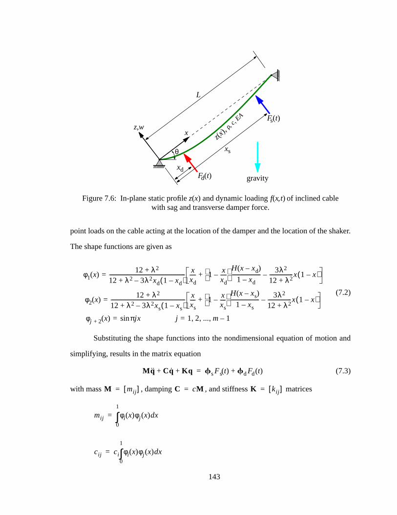
aker.
and
point loads on the cable acting at the location of the damper and the location of the sh
The shape functions are given as
(7.2)
Substituting the shape functions into the nondimensional equation of motion
simplifying, results in the matrix equation
(7.3)
with mass , damping , and stiffness matrices
Figure 7.6: In-plane static profilez(x) and dynamic loadingf(x,t) of inclined cablewith sag and transverse damper force.
z,wx
L
θ xs
Fd(t) gravity
z(x),
ρ,c,
EA Fs(t)
xd
φ1 x( )12 λ2+
12 λ2 3λ2xd 1 xd–( )–+---------------------------------------------------------- x
xd----- 1 x
xd-----–
H x xd–( )
1 xd–---------------------- 3λ2
12 λ2+------------------x 1 x–( )–+=
φ2 x( )12 λ2+
12 λ2 3λ2xs 1 xs–( )–+--------------------------------------------------------- x
xs---- 1 x
xs----–
H x xs–( )
1 xs–---------------------- 3λ2
12 λ2+------------------x 1 x–( )–+=
φj 2+ x( ) πjxsin= j 1 2 ... m 1–, , ,=
Mq Cq Kq+ + fsFs t( ) fdFd t( )+=
M mij[ ]= C cM= K kij[ ]=
mij φi x( )φj x( ) xd0
1
∫=
cij ci φi x( )φj x( ) xd0
1
∫=
143
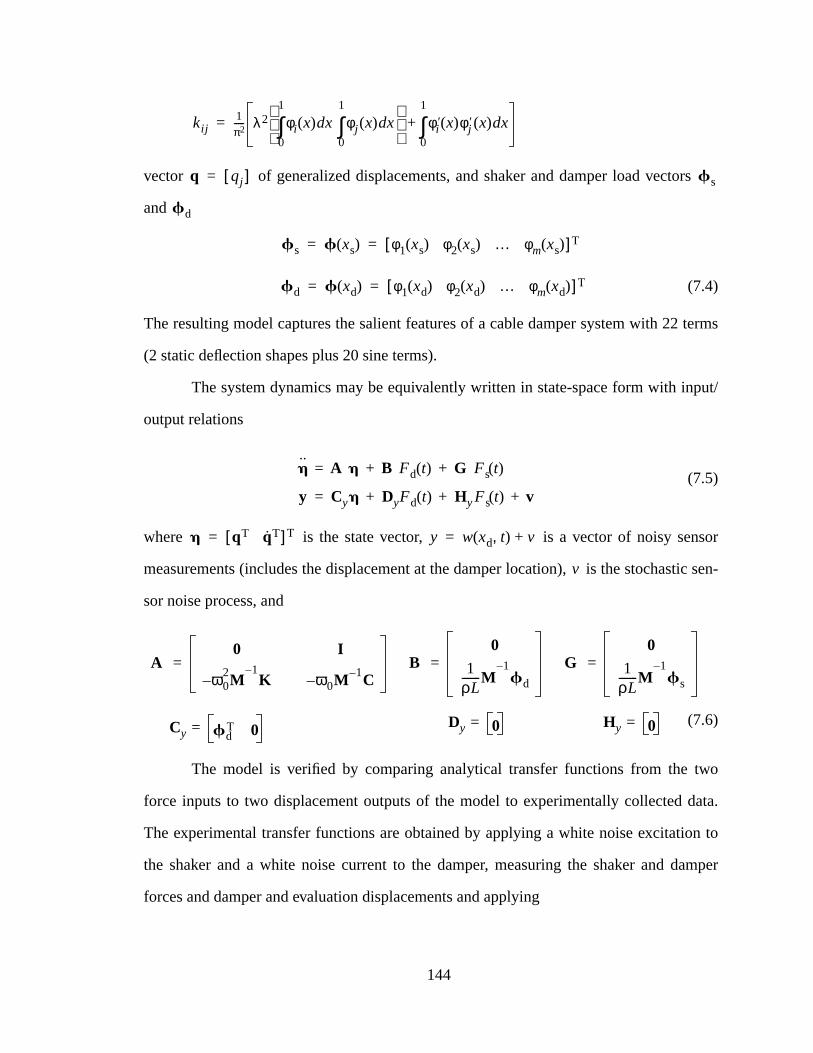
s
terms
put/
or
ic sen-
wo
data.
on to
amper
vector of generalized displacements, and shaker and damper load vector
and
(7.4)
The resulting model captures the salient features of a cable damper system with 22
(2 static deflection shapes plus 20 sine terms).
The system dynamics may be equivalently written in state-space form with in
output relations
(7.5)
where is the state vector, is a vector of noisy sens
measurements (includes the displacement at the damper location), is the stochast
sor noise process, and
(7.6)
The model is verified by comparing analytical transfer functions from the t
force inputs to two displacement outputs of the model to experimentally collected
The experimental transfer functions are obtained by applying a white noise excitati
the shaker and a white noise current to the damper, measuring the shaker and d
forces and damper and evaluation displacements and applying
kij1π2----- λ2 φi x( ) xd
0
1
∫ φj x( ) xd0
1
∫
φi′ x( )φj
′ x( ) xd0
1
∫+=
q qj[ ]= fs
fd
fs f xs( ) φ1 xs( ) φ2 xs( ) … φm xs( )[ ]T= =
fd f xd( ) φ1 xd( ) φ2 xd( ) … φm xd( )[ ]T= =
h = Azh + BzFd t( ) + GzFs t( )
y = Cyh + DyFd t( ) + HyFs t( ) + v
h qT qT[ ]T= y w xd t,( ) v+=
v
Az
0 I
ω02M
1–K– ω0M 1– C–
= Bz
0
1ρL-------M
1–fd
= Gz
0
1ρL-------M
1–fs
=
Cy fdT 0= Dy 0= Hy 0=
144
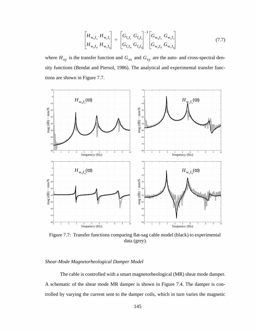
l den-
func-
per.
con-
netic
tal
(7.7)
where is the transfer function and and are the auto- and cross-spectra
sity functions (Bendat and Piersol, 1986). The analytical and experimental transfer
tions are shown in Figure 7.7.
Shear-Mode Magnetorheological Damper Model
The cable is controlled with a smart magnetorheological (MR) shear mode dam
A schematic of the shear mode MR damper is shown in Figure 7.4. The damper is
trolled by varying the current sent to the damper coils, which in turn varies the mag
HwdfsHwefs
HwdfdHwefd
Gf sfsGfdfs
Gf sfdGfdfd
1–Gwdfs
Gwefs
GwdfdGwefd
=
Hxy Gxx Gxy
0 1 2 3 4 5 6 7 8 9 10−80
−70
−60
−50
−40
−30
−20
−10
0
10
mag
(dB
) −
mm
/N
frequency (Hz)
0 1 2 3 4 5 6 7 8 9 10−80
−70
−60
−50
−40
−30
−20
−10
0
10
mag
(dB
) −
mm
/N
frequency (Hz)
0 1 2 3 4 5 6 7 8 9 10−80
−70
−60
−50
−40
−30
−20
−10
0
10
mag
(dB
) −
mm
/N
frequency (Hz)
0 1 2 3 4 5 6 7 8 9 10−80
−70
−60
−50
−40
−30
−20
−10
0
10
mag
(dB
) −
mm
/N
frequency (Hz)
Figure 7.7: Transfer functions comparing flat-sag cable model (black) to experimendata (grey).
Hwefsω( )Hwdfs
ω( )
Hwdfdω( ) Hwefd
ω( )
145
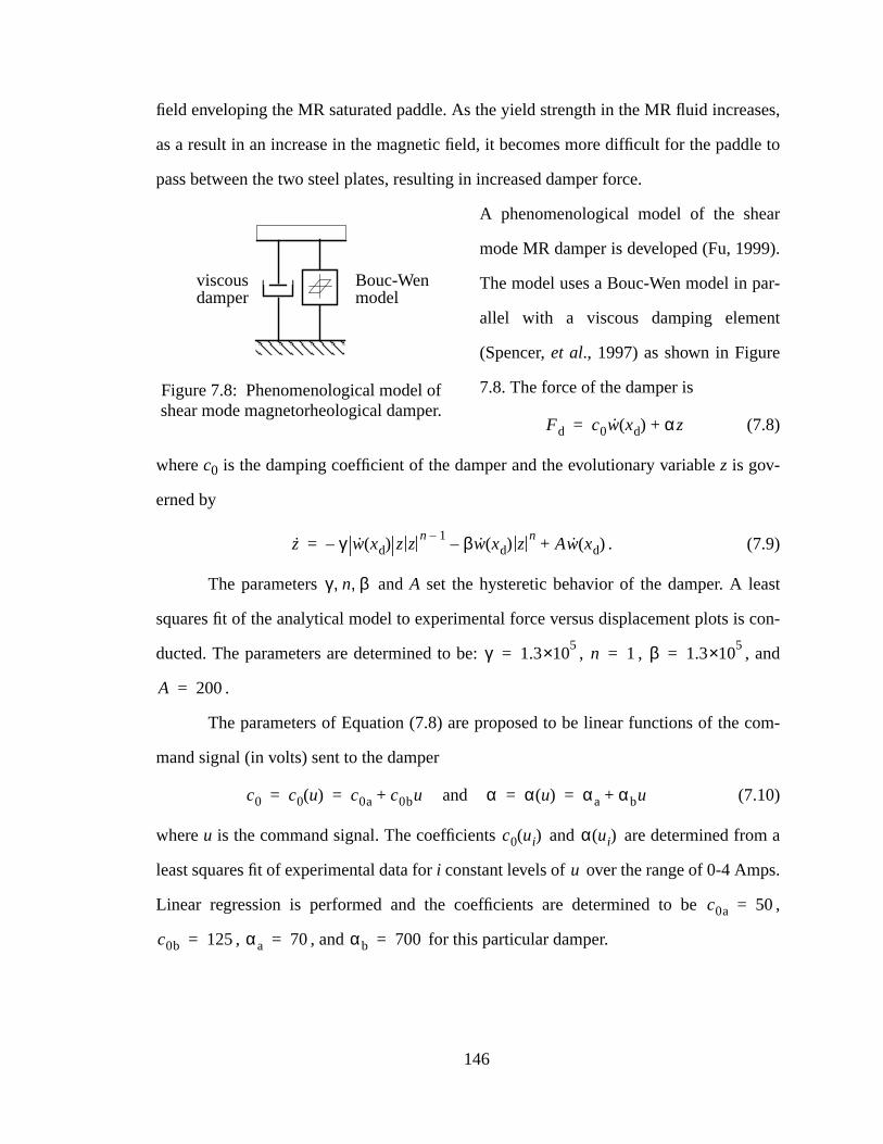
ses,
le to
r
).
r-
t
st
con-
and
com-
m a
s.
,
field enveloping the MR saturated paddle. As the yield strength in the MR fluid increa
as a result in an increase in the magnetic field, it becomes more difficult for the padd
pass between the two steel plates, resulting in increased damper force.
A phenomenological model of the shea
mode MR damper is developed (Fu, 1999
The model uses a Bouc-Wen model in pa
allel with a viscous damping elemen
(Spencer,et al., 1997) as shown in Figure
7.8. The force of the damper is
(7.8)
wherec0 is the damping coefficient of the damper and the evolutionary variablez is gov-
erned by
. (7.9)
The parameters andA set the hysteretic behavior of the damper. A lea
squares fit of the analytical model to experimental force versus displacement plots is
ducted. The parameters are determined to be: , , ,
.
The parameters of Equation (7.8) are proposed to be linear functions of the
mand signal (in volts) sent to the damper
and (7.10)
whereu is the command signal. The coefficients and are determined fro
least squares fit of experimental data fori constant levels of over the range of 0-4 Amp
Linear regression is performed and the coefficients are determined to be
, , and for this particular damper.
Figure 7.8: Phenomenological model ofshear mode magnetorheological damper.
viscousdamper
Bouc-Wenmodel
Fd c0w xd( ) αz+=
z γ w xd( ) z zn 1–
– βw xd( ) zn
– Aw xd( )+=
γ n β, ,
γ 1.35×10= n 1= β 1.3
5×10=
A 200=
c0 c0 u( ) c0a c0bu+= = α α u( ) αa αbu+= =
c0 ui( ) α ui( )
u
c0a 50=
c0b 125= αa 70= αb 700=
146
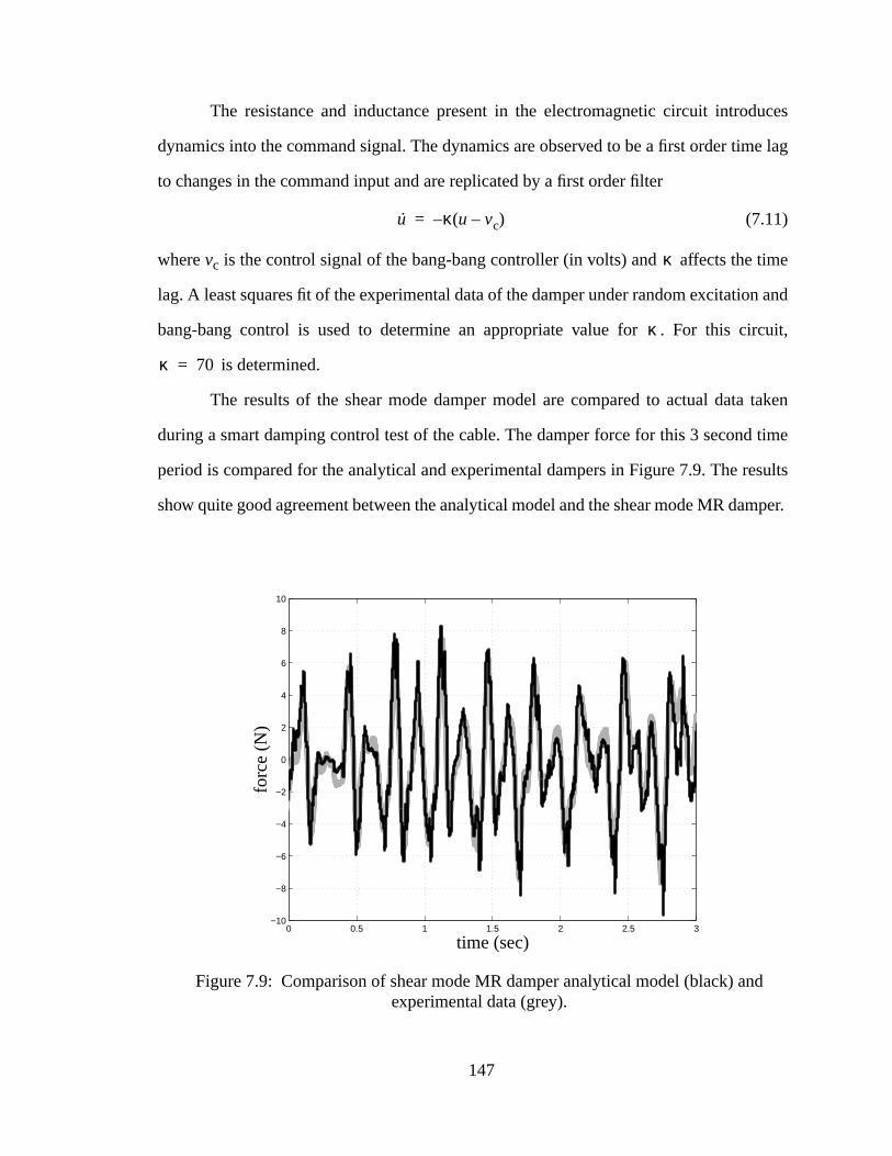
uces
e lag
ime
n and
cuit,
taken
time
sults
mper.
d
The resistance and inductance present in the electromagnetic circuit introd
dynamics into the command signal. The dynamics are observed to be a first order tim
to changes in the command input and are replicated by a first order filter
(7.11)
wherevc is the control signal of the bang-bang controller (in volts) and affects the t
lag. A least squares fit of the experimental data of the damper under random excitatio
bang-bang control is used to determine an appropriate value for . For this cir
is determined.
The results of the shear mode damper model are compared to actual data
during a smart damping control test of the cable. The damper force for this 3 second
period is compared for the analytical and experimental dampers in Figure 7.9. The re
show quite good agreement between the analytical model and the shear mode MR da
u κ u vc–( )–=
κ
κ
κ 70=
Figure 7.9: Comparison of shear mode MR damper analytical model (black) anexperimental data (grey).
0 0.5 1 1.5 2 2.5 3−10
−8
−6
−4
−2
0
2
4
6
8
10
forc
e (N
)
time (sec)
147
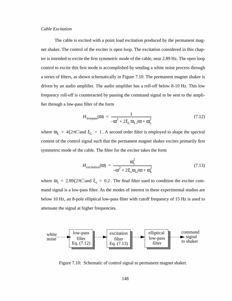
ag-
hap-
loop
ough
ker is
ow
mpli-
ctral
y first
m-
es are
to
Cable Excitation
The cable is excited with a point load excitation produced by the permanent m
net shaker. The control of the exciter is open loop. The excitation considered in this c
ter is intended to excite the first symmetric mode of the cable, near 2.89 Hz. The open
control to excite this first mode is accomplished by sending a white noise process thr
a series of filters, as shown schematically in Figure 7.10. The permanent magnet sha
driven by an audio amplifier. The audio amplifier has a roll-off below 8-10 Hz. This l
frequency roll-off is counteracted by passing the command signal to be sent to the a
fier through a low-pass filter of the form
(7.12)
where and . A second order filter is employed to shape the spe
content of the control signal such that the permanent magnet shaker excites primaril
symmetric mode of the cable. The filter for the exciter takes the form
(7.13)
where and . The final filter used to condition the exciter co
mand signal is a low-pass filter. As the modes of interest in these experimental studi
below 10 Hz, an 8-pole elliptical low-pass filter with cutoff frequency of 15 Hz is used
attenuate the signal at higher frequencies.
H lowpassω( ) 1
ω–2
2ξLωL jω ωL2
+ +-----------------------------------------------------=
ωL 4 2π( )= ξL 1=
Hexcitation ω( )ωs
2
ω–2
2ξsωs jω ωs2
+ +---------------------------------------------------=
ωs 2.89 2π( )= ξs 0.2=
Figure 7.10: Schematic of control signal to permanent magnet shaker.
low-pass elliptical commandsignal
to shaker
whitenoise filter
excitationfilter
filterEq. (7.12) Eq. (7.13)low-pass
148
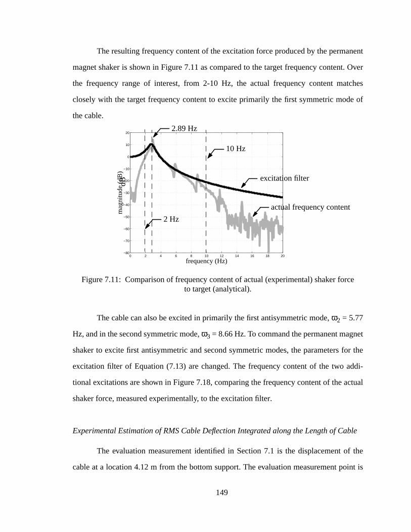
nent
. Over
tches
e of
et
or the
ddi-
ctual
ble
f the
int is
rce
The resulting frequency content of the excitation force produced by the perma
magnet shaker is shown in Figure 7.11 as compared to the target frequency content
the frequency range of interest, from 2-10 Hz, the actual frequency content ma
closely with the target frequency content to excite primarily the first symmetric mod
the cable.
The cable can also be excited in primarily the first antisymmetric mode,ω2 = 5.77
Hz, and in the second symmetric mode,ω3 = 8.66 Hz. To command the permanent magn
shaker to excite first antisymmetric and second symmetric modes, the parameters f
excitation filter of Equation (7.13) are changed. The frequency content of the two a
tional excitations are shown in Figure 7.18, comparing the frequency content of the a
shaker force, measured experimentally, to the excitation filter.
Experimental Estimation of RMS Cable Deflection Integrated along the Length of Ca
The evaluation measurement identified in Section 7.1 is the displacement o
cable at a location 4.12 m from the bottom support. The evaluation measurement po
0 2 4 6 8 10 12 14 16 18 20−80
−70
−60
−50
−40
−30
−20
−10
0
10
20
mag
nitu
de (
dB)
frequency (Hz)
Figure 7.11: Comparison of frequency content of actual (experimental) shaker foto target (analytical).
2.89 HzdB
excitation filter
actual frequency content
10 Hz
2 Hz
149
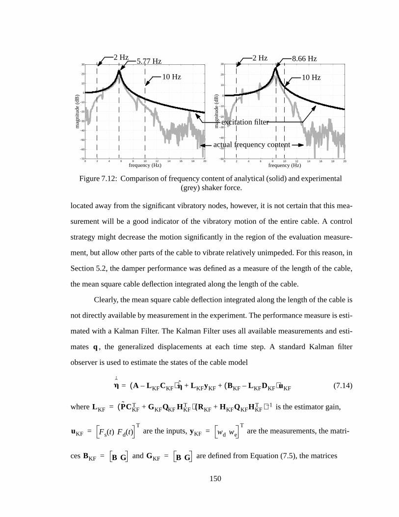
ea-
trol
sure-
n, in
cable,
ble is
s esti-
esti-
filter
tri-
l
located away from the significant vibratory nodes, however, it is not certain that this m
surement will be a good indicator of the vibratory motion of the entire cable. A con
strategy might decrease the motion significantly in the region of the evaluation mea
ment, but allow other parts of the cable to vibrate relatively unimpeded. For this reaso
Section 5.2, the damper performance was defined as a measure of the length of the
the mean square cable deflection integrated along the length of the cable.
Clearly, the mean square cable deflection integrated along the length of the ca
not directly available by measurement in the experiment. The performance measure i
mated with a Kalman Filter. The Kalman Filter uses all available measurements and
mates , the generalized displacements at each time step. A standard Kalman
observer is used to estimate the states of the cable model
(7.14)
where is the estimator gain,
are the inputs, are the measurements, the ma
ces and are defined from Equation (7.5), the matrices
0 2 4 6 8 10 12 14 16 18 20−70
−60
−50
−40
−30
−20
−10
0
10
20
30
mag
nitu
de (
dB)
frequency (Hz)0 2 4 6 8 10 12 14 16 18 20
−60
−50
−40
−30
−20
−10
0
10
20
30
mag
nitu
de (
dB)
frequency (Hz)
Figure 7.12: Comparison of frequency content of analytical (solid) and experimenta(grey) shaker force.
5.77 Hz
excitation filter
actual frequency content
10 Hz
2 Hz 8.66 Hz
10 Hz
2 Hz
q
h˙
A L KFCKF–( )h L KFyKF BKF L KFDKF–( )uKF+ +=
L KF PCKFT GKFQKF HKF
T+( ) RKF HKFQKFHKFT+( ) 1–=
uKF Fs t( ) Fd t( )T
= yKF wd we
T=
BKF B G= GKF B G=
150
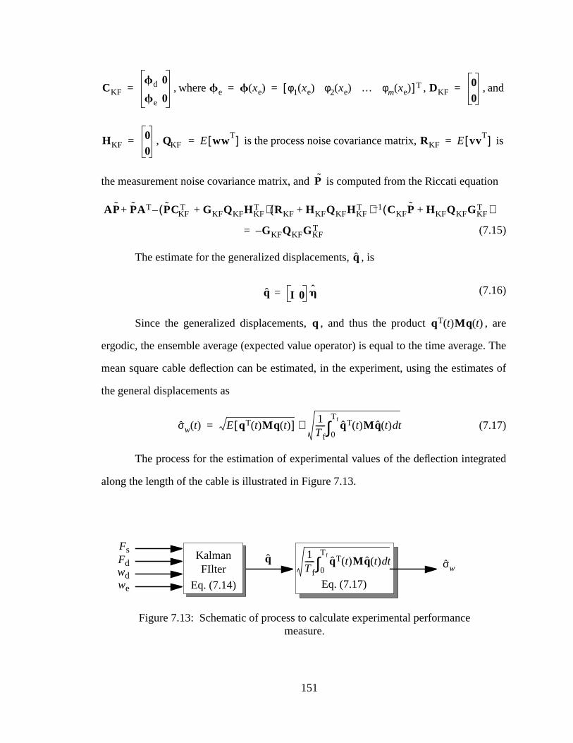
is
ation
, are
e. The
ates of
ated
, where , , and
, is the process noise covariance matrix,
the measurement noise covariance matrix, and is computed from the Riccati equ
(7.15)
The estimate for the generalized displacements, , is
(7.16)
Since the generalized displacements, , and thus the product
ergodic, the ensemble average (expected value operator) is equal to the time averag
mean square cable deflection can be estimated, in the experiment, using the estim
the general displacements as
(7.17)
The process for the estimation of experimental values of the deflection integr
along the length of the cable is illustrated in Figure 7.13.
CKFfd 0
fe 0= fe f xe( ) φ1 xe( ) φ2 xe( ) … φm xe( )[ ]T= = DKF
00
=
HKF00
= QKF E wwT[ ]= RKF E vvT[ ]=
P
AP PAT PCKFT GKFQKFHKF
T+( ) RKF HKF+ QKFHKFT ) 1– CKFP HKFQKFGKF
T+( )(–+
GKFQKFGKFT–=
q
q = I 0 h
q qT t( )Mq t( )
σw t( ) E qT t( )Mq t( )[ ] 1Tf----- qT t( )Mq t( ) td
0
Tf
∫≅=
Figure 7.13: Schematic of process to calculate experimental performancemeasure.
KalmanFIlter
1Tf----- qT t( )Mq t( ) td
0
Tf
∫Fd
Fs
we
wd
q σw
Eq. (7.14) Eq. (7.17)
151
, sup-
re the
ctive
ating
cable
rfor-
oltage
mpli-
oltage
and
ce is
ersus
mart
.14 it
of
lyt-
s var-
ing a
the
pti-
7.3 Passively-Operated Smart Damping Control Strategy
One method of operating smart cable dampers is in a purely passive capacity
plying the dampers with constant optimal voltage. The advantages to this strategy a
relative simplicity of implementing the control strategy as compared to a smart or a
control strategy and that the dampers are more easily optimally tuned in-place, elimin
the need to have passive dampers with unique optimal damping coefficients for each
of a cable-stayed bridge. The limitations to this method are the limited increase in pe
mance over optimally tuned passive dampers, and the dependence of the optimal v
on excitation magnitude and frequency content. The limited performance as well as a
tude and frequency dependence of the optimal passively-operated smart damping v
is shown in this section.
Amplitude Dependence
The dependence on the amplitude of the shaker force is shown in simulation
experimentally. Here the cable is excited in the first mode and the RMS shaker for
varied. The performance of the passively-operated smart damper control strategy v
damper voltage is plotted in Figure 7.14. Both the analytical curves, using the s
damper model of Section 7.2, and experimental points are presented. From Figure 7
is more clear that different damper voltages will be optimal for the different levels
shaker excitations.
The optimal voltage versus excitation level is shown in Figure 7.15, for the ana
ical and experimental systems. During experimental tests, voltage to the damper wa
ied in 0.2 volt increments. The experimental data verifies the analytical results, show
definite dependence of damper voltage on the level of excitation.
If the optimal passively-operated smart damping voltage is determined using
2 N RMS excitation level, the optimal voltage is 0. The performance of this system, o
152
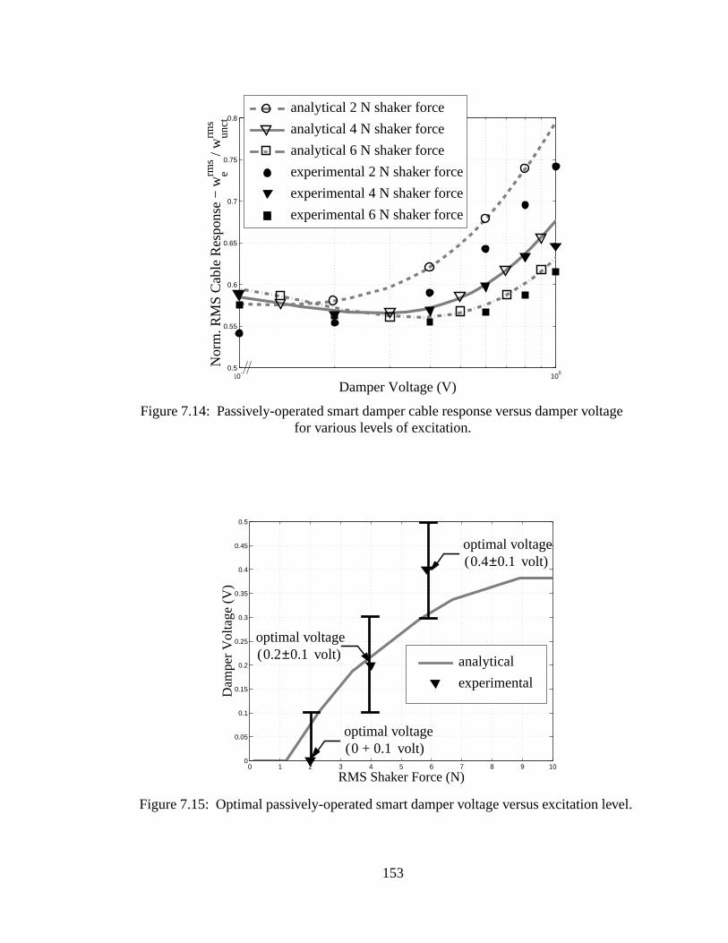
age
vel.
Figure 7.14: Passively-operated smart damper cable response versus damper voltfor various levels of excitation.
10−1
100
0.5
0.55
0.6
0.65
0.7
0.75
0.8
Damper Voltage (V)
Nor
m. R
MS
Cab
le R
espo
nse
− w erm
s / w
unct
rms
experimental 4 N shaker force
experimental 6 N shaker force
experimental 2 N shaker force
analytical 6 N shaker force
analytical 4 N shaker force
analytical 2 N shaker force
Figure 7.15: Optimal passively-operated smart damper voltage versus excitation le
0 1 2 3 4 5 6 7 8 9 100
0.05
0.1
0.15
0.2
0.25
0.3
0.35
0.4
0.45
0.5
RMS Shaker Force (N)
Dam
per
Vol
tage
(V
)
experimental
analytical
optimal voltage( volt)0.4 0.1±
optimal voltage( volt)0.2 0.1±
optimal voltage( volt)0 0.1+
153
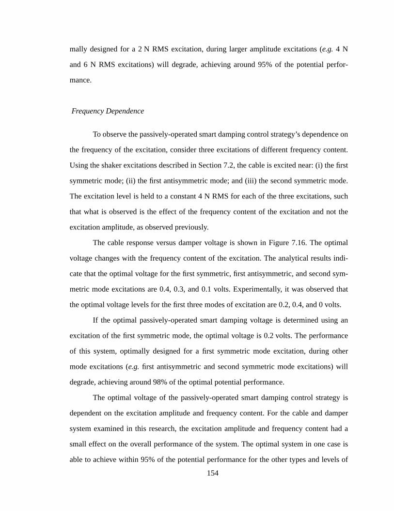
rfor-
ce on
tent.
e first
ode.
h
t the
timal
indi-
sym-
that
olts.
g an
nce
ther
ill
gy is
amper
had a
se is
ls of
mally designed for a 2 N RMS excitation, during larger amplitude excitations (e.g.4 N
and 6 N RMS excitations) will degrade, achieving around 95% of the potential pe
mance.
Frequency Dependence
To observe the passively-operated smart damping control strategy’s dependen
the frequency of the excitation, consider three excitations of different frequency con
Using the shaker excitations described in Section 7.2, the cable is excited near: (i) th
symmetric mode; (ii) the first antisymmetric mode; and (iii) the second symmetric m
The excitation level is held to a constant 4 N RMS for each of the three excitations, suc
that what is observed is the effect of the frequency content of the excitation and no
excitation amplitude, as observed previously.
The cable response versus damper voltage is shown in Figure 7.16. The op
voltage changes with the frequency content of the excitation. The analytical results
cate that the optimal voltage for the first symmetric, first antisymmetric, and second
metric mode excitations are 0.4, 0.3, and 0.1 volts. Experimentally, it was observed
the optimal voltage levels for the first three modes of excitation are 0.2, 0.4, and 0 v
If the optimal passively-operated smart damping voltage is determined usin
excitation of the first symmetric mode, the optimal voltage is 0.2 volts. The performa
of this system, optimally designed for a first symmetric mode excitation, during o
mode excitations (e.g.first antisymmetric and second symmetric mode excitations) w
degrade, achieving around 98% of the optimal potential performance.
The optimal voltage of the passively-operated smart damping control strate
dependent on the excitation amplitude and frequency content. For the cable and d
system examined in this research, the excitation amplitude and frequency content
small effect on the overall performance of the system. The optimal system in one ca
able to achieve within 95% of the potential performance for the other types and leve
154
on of
cant
sively-
l is
force
sign;
pri-
ltage
excitation. However, different cables and different dampers, as well as a combinati
different amplitude and frequency changes in the excitation, may result in more signifi
loss of performance. These concerns should be considered when applying the pas
operated smart damper control strategy.
7.4 Experimental Semiactive Cable Damping Control Strategy
An ideal controllable-fluid damper (Spencer and Sain, 1997; Housneret al., 1997)
can only exertdissipativeforces. For control design, a generic semiactive device mode
assumed that is purely dissipative. Essentially, this requirement dictates that the
exerted by the damper and the velocity across the damper must be of opposite
i.e., must be less than zero. A clipped optimal strategy is used, with a
Figure 7.16: Passively-operated smart damper cable response versus damper vofor various modes excited.
10−1
100
0.5
0.55
0.6
0.65
0.7
0.75
0.8
0.85
0.9
Damper Voltage (V)
Nor
m. R
MS
Cab
le R
espo
nse
− w erm
s / w
unct
rms exp. first antisymmetric excited
exp. second symmetric excited
exp. first symmetric excited
analytical third mode excited
analytical second mode excited
analytical first mode excited
Fd t( )w xd t,( )
155
r the
cable
s of
a non-
than
es in
ance
luation
cable
pri-
s
em,
mary controller based on an LQG design and a secondary controller to account fo
nonlinear nature of the semiactive device. The controller is designed to reduce the
displacement over the length of the cable.
Control Objective
Modal damping ratios provide a useful means of determining the effectivenes
linear viscous damping strategies. However, using a semiactive damper introduces
linearity into the combined system. Consequently, performance measures other
modal damping must be used for judging the efficacy of nonlinear damping strategi
comparison with linear (passive or active) dampers. The measure of damper perform
considered herein is the square root of the mean square cable deflection at the eva
point (4.12 m from the bottom support) and the square root of the mean square
deflection integrated along the length of the cable, as estimated with a Kalman filter.
Primary Controller
An H2/LQG control design, as presented in Section 5.3, is considered for the
mary controller of the cable experiment. The cost function employed here is given a
(7.18)
A second order filter is augmented to the model of the structural syst
Equation (7.5), to weight the spectral content of the shaker excitation in theH2/LQG con-
trol design. The second order filter is
(7.19)
J1 σdisplacement2 Rσforce
2+ E1T--- qTMq R Fd
2+( ) td0
T
∫T ∞→lim= =
Hdesignω( )ωf
2
ω–2
2ξfωf jω ωf2
+ +--------------------------------------------------=
156
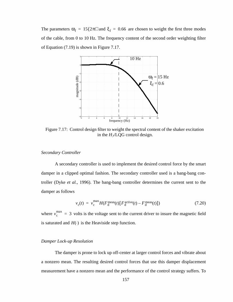
des
filter
mart
con-
the
field
bout
ement
ers. To
tion
The parameters and are chosen to weight the first three mo
of the cable, from 0 to 10 Hz. The frequency content of the second order weighting
of Equation (7.19) is shown in Figure 7.17.
Secondary Controller
A secondary controller is used to implement the desired control force by the s
damper in a clipped optimal fashion. The secondary controller used is a bang-bang
troller (Dyke et al., 1996). The bang-bang controller determines the current sent to
damper as follows
(7.20)
where volts is the voltage sent to the current driver to insure the magnetic
is saturated and is the Heaviside step function.
Damper Lock-up Resolution
The damper is prone to lock up off-center at larger control forces and vibrate a
a nonzero mean. The resulting desired control forces that use this damper displac
measurement have a nonzero mean and the performance of the control strategy suff
ωf 15 2π( )= ξf 0.66=
0 2 4 6 8 10 12 14 16 18 20−6
−5
−4
−3
−2
−1
0
1
mag
nitu
de (
dB)
frequency (Hz)
Figure 7.17: Control design filter to weight the spectral content of the shaker excitain theH2/LQG control design.
ωf = 15 Hz
ξf = 0.6
10 Hz
vc t( ) vcmax
H Fdmeast( ) Fd
active t( ) Fdmeast( )–[ ]( )=
vcmax
3=
H .( )
157
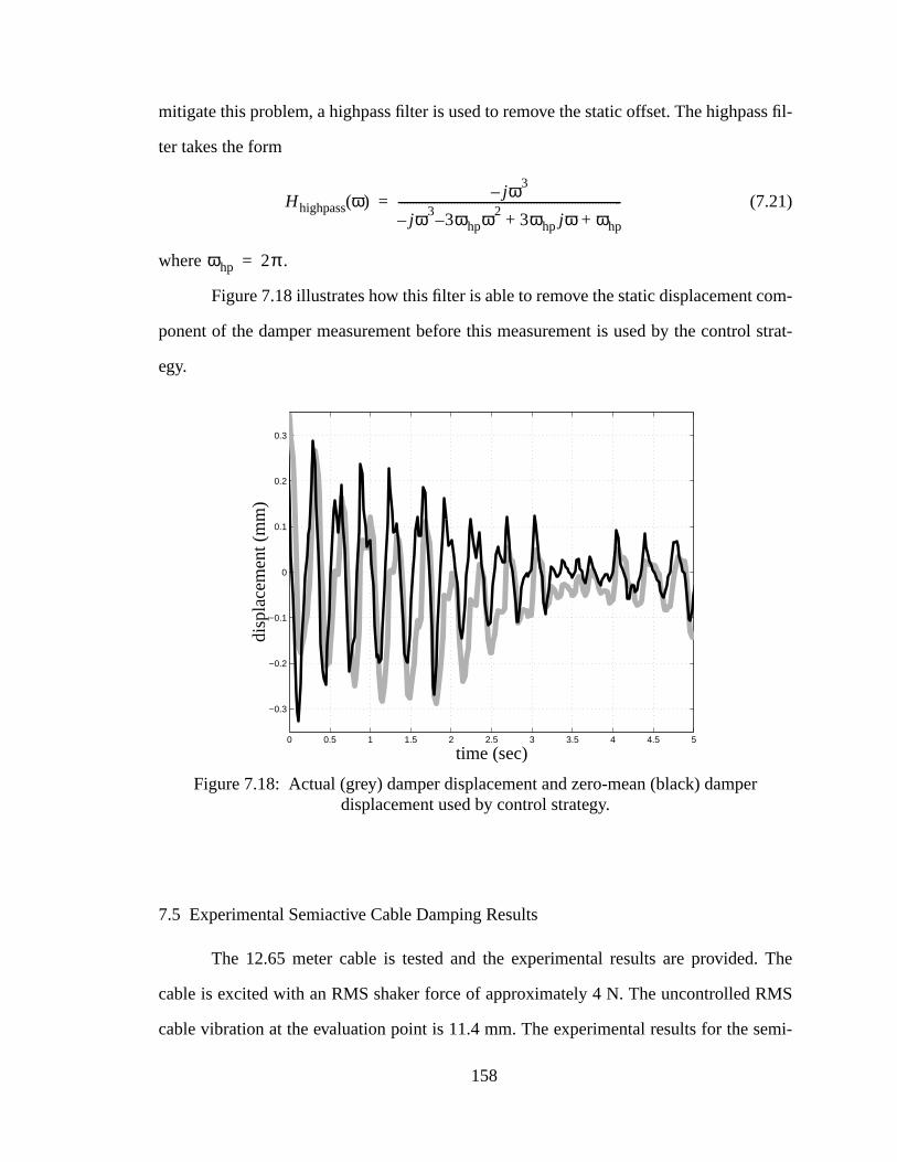
ss fil-
om-
l strat-
. The
MS
emi-
r
mitigate this problem, a highpass filter is used to remove the static offset. The highpa
ter takes the form
(7.21)
where .
Figure 7.18 illustrates how this filter is able to remove the static displacement c
ponent of the damper measurement before this measurement is used by the contro
egy.
7.5 Experimental Semiactive Cable Damping Results
The 12.65 meter cable is tested and the experimental results are provided
cable is excited with an RMS shaker force of approximately 4 N. The uncontrolled R
cable vibration at the evaluation point is 11.4 mm. The experimental results for the s
Hhighpassω( ) jω–3
jω–3
3– ωhpω23ωhp jω ωhp+ +
----------------------------------------------------------------------------=
ωhp 2π=
Figure 7.18: Actual (grey) damper displacement and zero-mean (black) dampedisplacement used by control strategy.
0 0.5 1 1.5 2 2.5 3 3.5 4 4.5 5
−0.3
−0.2
−0.1
0
0.1
0.2
0.3
disp
lace
men
t (m
m)
time (sec)
158
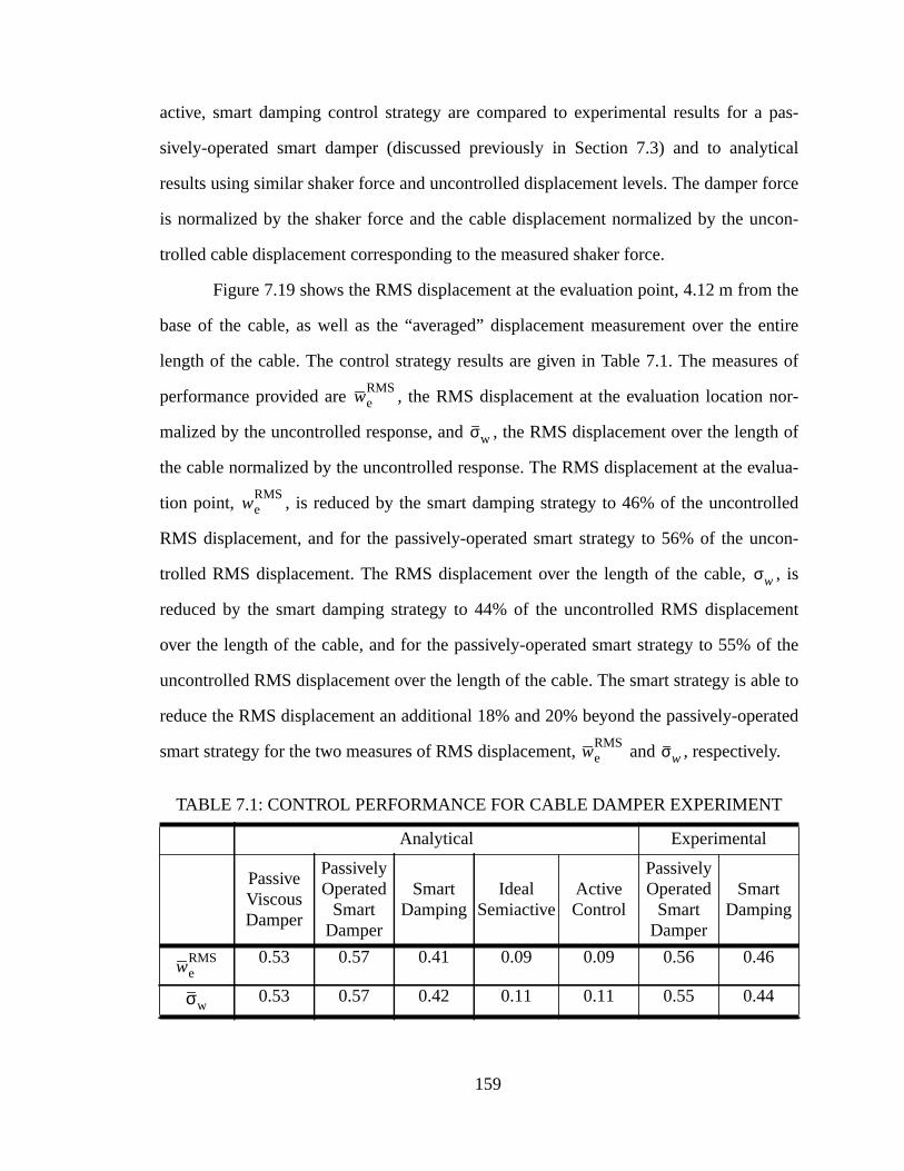
pas-
ytical
force
ncon-
the
entire
res of
nor-
th of
valua-
lled
ncon-
, is
ment
of the
ble to
erated
ely.
active, smart damping control strategy are compared to experimental results for a
sively-operated smart damper (discussed previously in Section 7.3) and to anal
results using similar shaker force and uncontrolled displacement levels. The damper
is normalized by the shaker force and the cable displacement normalized by the u
trolled cable displacement corresponding to the measured shaker force.
Figure 7.19 shows the RMS displacement at the evaluation point, 4.12 m from
base of the cable, as well as the “averaged” displacement measurement over the
length of the cable. The control strategy results are given in Table 7.1. The measu
performance provided are , the RMS displacement at the evaluation location
malized by the uncontrolled response, and , the RMS displacement over the leng
the cable normalized by the uncontrolled response. The RMS displacement at the e
tion point, , is reduced by the smart damping strategy to 46% of the uncontro
RMS displacement, and for the passively-operated smart strategy to 56% of the u
trolled RMS displacement. The RMS displacement over the length of the cable,
reduced by the smart damping strategy to 44% of the uncontrolled RMS displace
over the length of the cable, and for the passively-operated smart strategy to 55%
uncontrolled RMS displacement over the length of the cable. The smart strategy is a
reduce the RMS displacement an additional 18% and 20% beyond the passively-op
smart strategy for the two measures of RMS displacement, and , respectiv
TABLE 7.1: CONTROL PERFORMANCE FOR CABLE DAMPER EXPERIMENT
Analytical Experimental
PassiveViscousDamper
PassivelyOperated
SmartDamper
SmartDamping
IdealSemiactive
ActiveControl
PassivelyOperated
SmartDamper
SmartDamping
0.53 0.57 0.41 0.09 0.09 0.56 0.46
0.53 0.57 0.42 0.11 0.11 0.55 0.44
weRMS
σw
weRMS
σw
weRMS σw
weRMS
σw
159
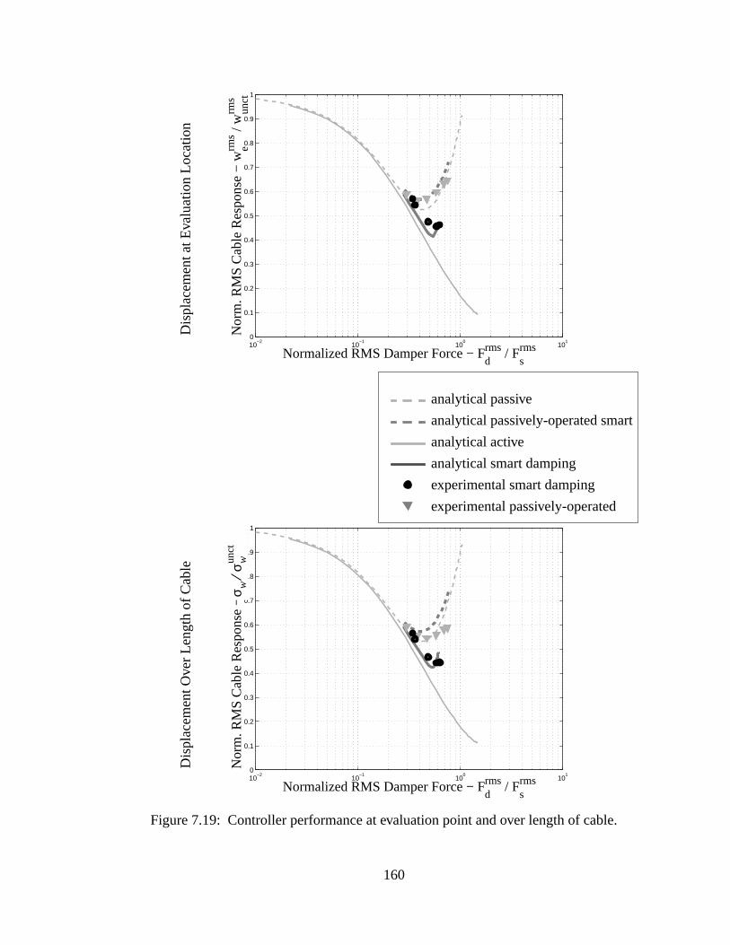
.
Figure 7.19: Controller performance at evaluation point and over length of cable10−2
10−1
100
101
0
0.1
0.2
0.3
0.4
0.5
0.6
0.7
0.8
0.9
1
Normalized RMS Damper Force − Fdrms / F
srms
Nor
m. R
MS
Cab
le R
espo
nse
− w erm
s / w
unct
rms
10−2
10−1
100
101
0
0.1
0.2
0.3
0.4
0.5
0.6
0.7
0.8
0.9
1
Normalized RMS Damper Force − Fdrms / F
srms
Nor
m. R
MS
Cab
le R
espo
nse
− w erm
s / w
unct
rms
Dis
plac
emen
t at E
valu
atio
n Lo
catio
nD
ispl
acem
ent O
ver
Leng
th o
f Cab
le
experimental smart damping
experimental passively-operated
analytical smart damping
analytical active
analytical passively-operated smart
analytical passive
σ wσ wun
ct⁄
160
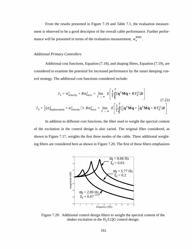
sure-
erfor-
, are
g con-
tent
, as
ight-
asizes
e
From the results presented in Figure 7.19 and Table 7.1, the evaluation mea
ment is observed to be a good descriptor of the overall cable performance. Further p
mance will be presented in terms of the evaluation measurement, .
Additional Primary Controllers
Additional cost functions, Equation (7.18), and shaping filters, Equation (7.19)
considered to examine the potential for increased performance by the smart dampin
trol strategy. The additional cost functions considered include:
(7.22)
In addition to different cost functions, the filter used to weight the spectral con
of the excitation in the control design is also varied. The original filter considered
shown in Figure 7.17, weights the first three modes of the cable. Three additional we
ing filters are considered here as shown in Figure 7.20. The first of these filters emph
weRMS
J2 σvelocity2 Rσforce
2+ E1T--- qTMq R Fd
2+( ) td0
T
∫T ∞→lim= =
J412--- σdisplacement
2 σvelocity2+( ) Rσforce
2+ E1T--- 1
2---qTMq 1
2---qTMq R Fd
2+ +( ) td0
T
∫T ∞→lim= =
0 2 4 6 8 10 12 14 16 18 20−40
−30
−20
−10
0
10
20
30
mag
nitu
de (
dB)
frequency (Hz)
Figure 7.20: Additional control design filters to weight the spectral content of thshaker excitation in theH2/LQG control design.
ωf = 2.89 Hzξf = 0.07
ωf = 5.77 Hzξf = 0.2
ωf = 8.66 Hzξf = 0.03
161
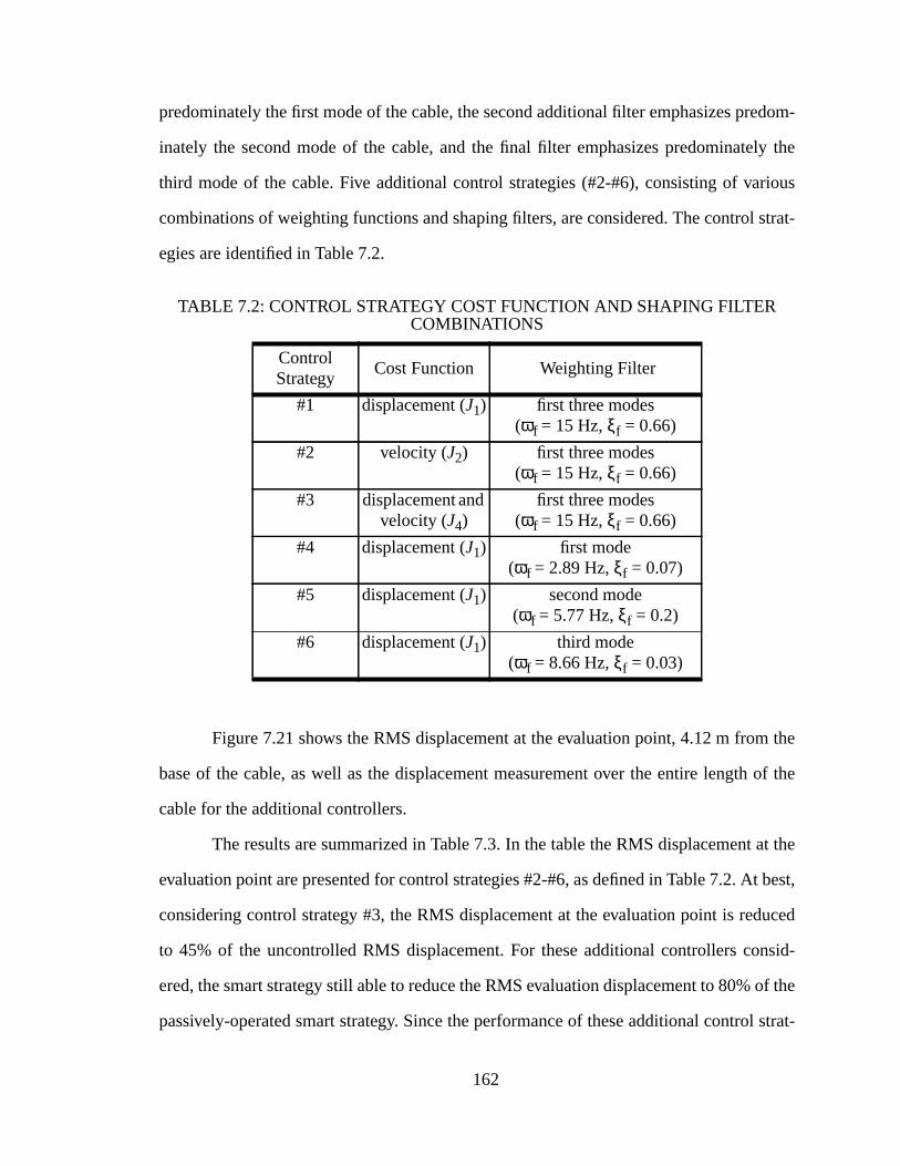
dom-
ly the
ious
strat-
the
of the
at the
t best,
uced
nsid-
of the
l strat-
predominately the first mode of the cable, the second additional filter emphasizes pre
inately the second mode of the cable, and the final filter emphasizes predominate
third mode of the cable. Five additional control strategies (#2-#6), consisting of var
combinations of weighting functions and shaping filters, are considered. The control
egies are identified in Table 7.2.
Figure 7.21 shows the RMS displacement at the evaluation point, 4.12 m from
base of the cable, as well as the displacement measurement over the entire length
cable for the additional controllers.
The results are summarized in Table 7.3. In the table the RMS displacement
evaluation point are presented for control strategies #2-#6, as defined in Table 7.2. A
considering control strategy #3, the RMS displacement at the evaluation point is red
to 45% of the uncontrolled RMS displacement. For these additional controllers co
ered, the smart strategy still able to reduce the RMS evaluation displacement to 80%
passively-operated smart strategy. Since the performance of these additional contro
TABLE 7.2: CONTROL STRATEGY COST FUNCTION AND SHAPING FILTERCOMBINATIONS
ControlStrategy
Cost Function Weighting Filter
#1 displacement (J1) first three modes(ωf = 15 Hz,ξf = 0.66)
#2 velocity (J2) first three modes(ωf = 15 Hz,ξf = 0.66)
#3 displacement andvelocity (J4)
first three modes(ωf = 15 Hz,ξf = 0.66)
#4 displacement (J1) first mode(ωf = 2.89 Hz,ξf = 0.07)
#5 displacement (J1) second mode(ωf = 5.77 Hz,ξf = 0.2)
#6 displacement (J1) third mode(ωf = 8.66 Hz,ξf = 0.03)
162
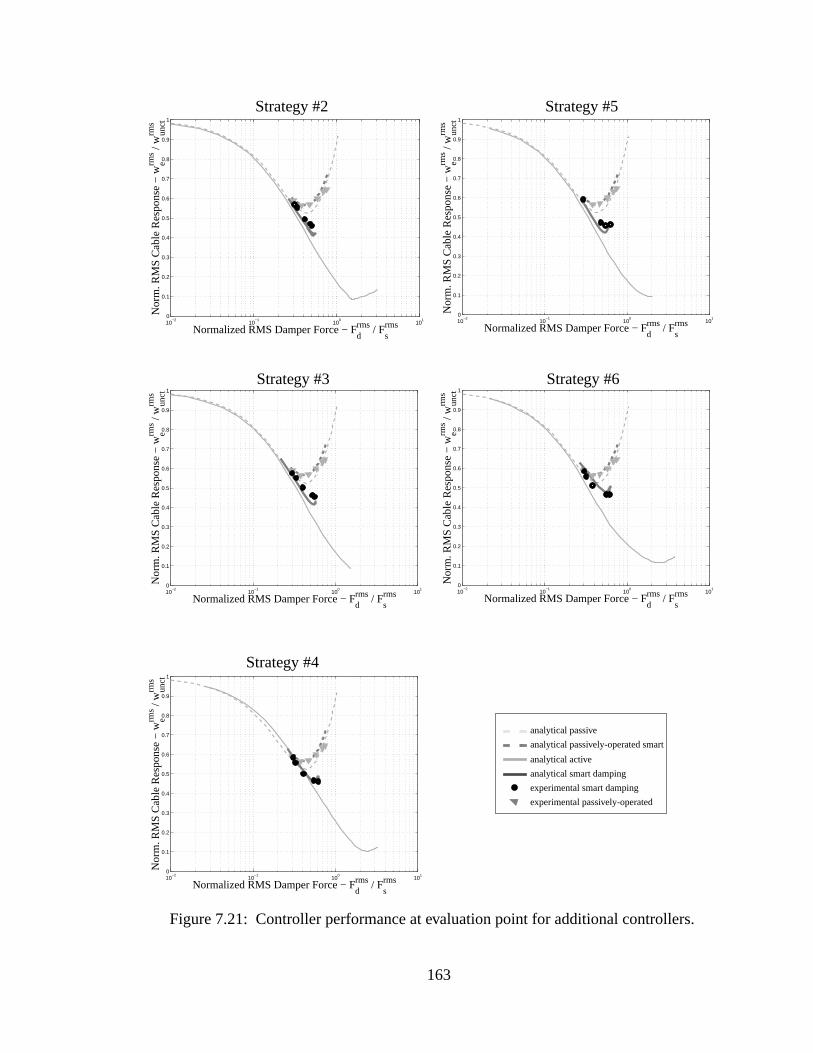
.
10−2
10−1
100
101
0
0.1
0.2
0.3
0.4
0.5
0.6
0.7
0.8
0.9
1
Normalized RMS Damper Force − Fdrms / F
srms
Nor
m. R
MS
Cab
le R
espo
nse
− w erm
s / w
unct
rms
10−2
10−1
100
101
0
0.1
0.2
0.3
0.4
0.5
0.6
0.7
0.8
0.9
1
Normalized RMS Damper Force − Fdrms / F
srms
Nor
m. R
MS
Cab
le R
espo
nse
− w erm
s / w
unct
rms
10−2
10−1
100
101
0
0.1
0.2
0.3
0.4
0.5
0.6
0.7
0.8
0.9
1
Normalized RMS Damper Force − Fdrms / F
srms
Nor
m. R
MS
Cab
le R
espo
nse
− w erm
s / w
unct
rms
10−2
10−1
100
101
0
0.1
0.2
0.3
0.4
0.5
0.6
0.7
0.8
0.9
1
Normalized RMS Damper Force − Fdrms / F
srms
Nor
m. R
MS
Cab
le R
espo
nse
− w erm
s / w
unct
rms
10−2
10−1
100
101
0
0.1
0.2
0.3
0.4
0.5
0.6
0.7
0.8
0.9
1
Normalized RMS Damper Force − Fdrms / F
srms
Nor
m. R
MS
Cab
le R
espo
nse
− w erm
s / w
unct
rms
Figure 7.21: Controller performance at evaluation point for additional controllers
experimental smart damping
experimental passively-operated
analytical smart damping
analytical active
analytical passively-operated smart
analytical passive
Strategy #2 Strategy #5
Strategy #3 Strategy #6
Strategy #4
163

e for
om-
mper is
linear
ment
cable
egies is similar, selecting one control strategy, namely the first control strategy, is don
further studies.
Additional Cable Excitation
The performance of the smart damper, using the first control strategy (#1) is c
pared to analytical results as well as a passive strategy whereby the shear mode da
supplied varying levels of constant current such that the damper behaves as a non
passive damper. The controller performance is illustrated in Figure 7.22.
The results are summarized in Table 7.4. In the table both the RMS displace
at the evaluation point and the estimated RMS displacement over the length of the
are presented.
TABLE 7.3: CONTROL PERFORMANCE, , FOR ADDITIONAL CONTROLSTRATEGIES
ControlStrategy
ANALYTICAL
SmartDamping
EXPERIMENTAL
SmartDamping
#2 0.41 0.46#3 0.41 0.45#4 0.46 0.46#5 0.42 0.46#6 0.48 0.46
TABLE 7.4: CONTROL PERFORMANCE, ( ), FOR 1ST ANTISYMMETRICAND 2ND SYMMETRIC MODE EXCITATIONS
Excitation Analytical Experimental
PassiveViscousDamper
PassivelyOperated
SmartDamper
SmartDamping
IdealSemiactive
ActiveControl
PassivelyOperated
SmartDamper
SmartDamping
1st antisymmetric 0.61 0.64 0.51 0.12 0.64 0.512nd symmetric 0.69 0.69 0.58 0.49 0.70 0.58
weRMS
weRMS
164
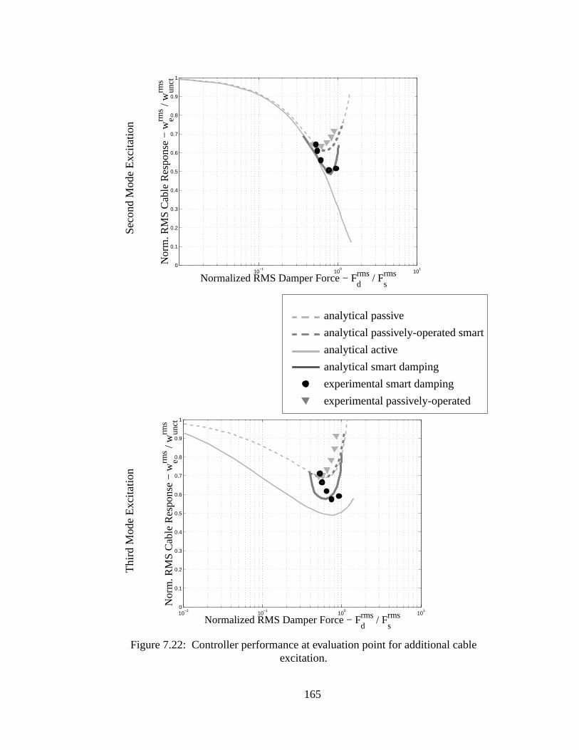
10−1
100
101
0
0.1
0.2
0.3
0.4
0.5
0.6
0.7
0.8
0.9
1
Normalized RMS Damper Force − Fdrms / F
srms
Nor
m. R
MS
Cab
le R
espo
nse
− w erm
s / w
unct
rms
10−2
10−1
100
101
0
0.1
0.2
0.3
0.4
0.5
0.6
0.7
0.8
0.9
1
Normalized RMS Damper Force − Fdrms / F
srms
Nor
m. R
MS
Cab
le R
espo
nse
− w erm
s / w
unct
rms
Figure 7.22: Controller performance at evaluation point for additional cableexcitation.
Sec
ond
Mod
e E
xcita
tion
Thi
rd M
ode
Exc
itatio
n
experimental smart damping
experimental passively-operated
analytical smart damping
analytical active
analytical passively-operated smart
analytical passive
165
point
dis-
spec-
64%
anti-
met-
RMS
ively-
ntrol
ation
e con-
e mea-
rol is
lting
g the
e sig-
odel,
eyond
olves
litude
ticu-
The experimental results show that the RMS displacement at the evaluation
for the smart damping strategy is reduced to 51% and 58% of the uncontrolled RMS
placement for the first antisymmetric and second symmetric mode excitations, re
tively. The passively-operated smart strategy is able to reduce the displacement to
and 70% of uncontrolled RMS displacement at the evaluation location for the first
symmetric and second symmetric mode excitations, respectively. For the first antisym
ric and second symmetric mode excitations, the smart strategy is able to reduce the
evaluation displacement, , an additional 20% and 17% beyond that of the pass
operated smart strategy.
7.6 Chapter Summary
In this chapter, a 12.65 m flat-sag cable is implemented with a semiactive co
strategy employing a shear mode magnetorheological fluid damper. System identific
is performed and models for the cable and smart damper are developed. A semiactiv
trol strategy is proposed and implemented that uses damper displacement and forc
surements for feedback control. A practical issue observed in implementing the cont
when the damper locks up off-center and begins vibrating about off-center point, resu
in a loss of control performance. The off-center vibration issue is resolved by passin
measurement signals through a highpass filter, eliminating the DC component of th
nal. Experimental results are confirmed by analytical studies including the damper m
that smart cable damping achieves reduces cable displacement an additional 20% b
the performance of passive control. The passive control examined experimentally inv
sending a constant control signal to the smart damper. The frequency and amp
dependency of this control strategy are identified; although not significant for this par
lar cable system, this dependency should be considered on a case by case basis.
weRMS
166

sec-
In the next chapter, Chapter 8, control-structure interaction, identified in thistion, is examined in further detail.
167
was
inves-
dered
mula-
ined.
ance
ts of
cable
nk at
the
tant to
ntrol.
l used
7. The
. An
physi-
ngent
cable
l and
CHAPTER 8: INVESTIGATING EXPERIMENTAL AND SIMULATION CABLE
DAMPING CONTROL PERFORMANCE
The experimental and smart damping simulation performance of Chapter 7
shown to be less than the ideal semiactive damper studied in Chapter 6. This chapter
tigates factors that may explain the difference in performance. Two factors are consi
to have a possible effect. First, the bending stiffness of the cable, neglected in the si
tion studies, is examined. Next, the properties of the semiactive damper are exam
This investigation offers an explanation to the difference in cable damping perform
and suggests a solution to experimentally regain this performance.
The analytical cable model developed in Chapter 5 and the simulation resul
Chapters 6 and 7 consider a flat-sag cable model where the bending stiffness of the
is neglected. The point load of the damper acting on the cable model will result in a ki
the point of application. Cable bending stiffness reduces this kinking action. Since
actual cable used in the experiment has an associated bending stiffness, it is impor
consider the effect of the bending stiffness on the performance of cable damping co
The second factor investigated is the difference between the ideal cable mode
in Chapter 6 and the shear mode magnetorheological (MR) damper used in Chapter
issue of controller discretization is identified and the effect on the control studied
alternative arctangent damper model is considered to be more representative of the
cal system than the ideal model. A stiffness element is added in series to the arcta
damper model to observe the effect of device compliance on the performance of the
damper. The investigation provides insight for future damper design for experimenta
full-scale cable damping control strategies.
168
r the
d, as
oint
pe of
ction,
t of
nder
d by
sec,
first
shows
show
le at
r to
inate
ness
mance
erve
mea-
8.1 Investigating Cable Bending Stiffness
When damper forces are applied to the cable, the cable deforms locally. Fo
analytical cable model developed in Chapter 5 where bending stiffness is neglecte
well as in previous studies of cable damping (Fujinoet al. 1993, 1994, 1995, Johnson
et al.2000c, 2001a, 2001b), the cable is allowed to form a kink at the location of the p
load. Physically, with some bending stiffness inherently present in the cable, the slo
the cable deflection cannot be discontinuous, as required to form a kink. In this se
bending stiffness is included in the cable model to examine, analytically, the effec
cable bending stiffness on cable damping control.
Figure 8.1 shows the cable model of Chapter 7 without bending stiffness u
control with a damper located at 2% the total length of the cable (the cable is excite
another point load at the shaker at ). The first profile shown is at time 3.35
just prior to the control force being applied to the cable. This profile represents the
mode vibration of the cable, supported at both ends. The second profile, at 3.36 sec,
the cable just as the control force is applied. The next two profiles at 3.4 and 3.45 sec
the cable with an applied control force and the resulting kink that is formed in the cab
the location of the cable damper. When the control force is turned off, just prio
3.50 sec, the kink disappears. Including bending stiffness in the cable model will elim
the kinking that occurs at the damper. In what follows, the effect of cable bending stiff
on passive and active cable damping control are examined as they bound the perfor
of semiactive “smart” cable damping control.
Flat-Sag Cable Model Incorporating Bending Stiffness
Bending stiffness typical for stay cables is included in the cable model to obs
the effect on cable damping control. The nondimensional parameter is used as a
sure of the bending stiffness and is defined as:
x 0.97=
1 γ⁄
169
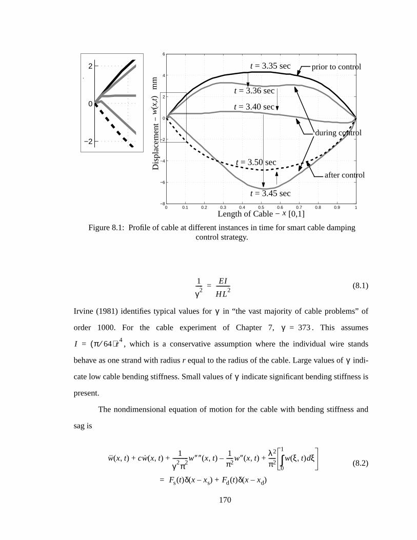
of
mes
nds
i-
ss is
and
g
(8.1)
Irvine (1981) identifies typical values for in “the vast majority of cable problems”
order 1000. For the cable experiment of Chapter 7, . This assu
, which is a conservative assumption where the individual wire sta
behave as one strand with radiusr equal to the radius of the cable. Large values of ind
cate low cable bending stiffness. Small values of indicate significant bending stiffne
present.
The nondimensional equation of motion for the cable with bending stiffness
sag is
(8.2)
0 0.1 0.2 0.3 0.4 0.5 0.6 0.7 0.8−8
−6
−4
−2
0
2
Length of Cable− x [0,1]
Dis
plac
emen
t − w
(mm
) t = 3.36 sec
t = 3.40 sec
t = 3.45 sec
t = 3.50 sec
0 0.1 0.2 0.3 0.4 0.5 0.6 0.7 0.8 0.9 1−8
−6
−4
−2
0
2
4
6
Length of Cable − x [0,1]
Dis
plac
emen
t − w
(m
m)
Figure 8.1: Profile of cable at different instances in time for smart cable dampincontrol strategy.
t = 3.35 sec
t = 3.36 sec
t = 3.40 sec
t = 3.45 sec
t = 3.50 sec
during control
prior to control
after control
x
w(x
,t)m
m
1
γ2----- EI
HL2
----------=
γ
γ 373=
I π 64⁄( )r4=
γ
γ
w x t,( ) cw x t,( )1
γ2π2-----------w″″ x t,( )
1π2-----w″ x t,( )–
λ2
π2----- w ξ t,( ) ξd
0
1
∫+ + +
Fs t( )δ x xs–( ) Fd t( )δ x xd–( )+=
170
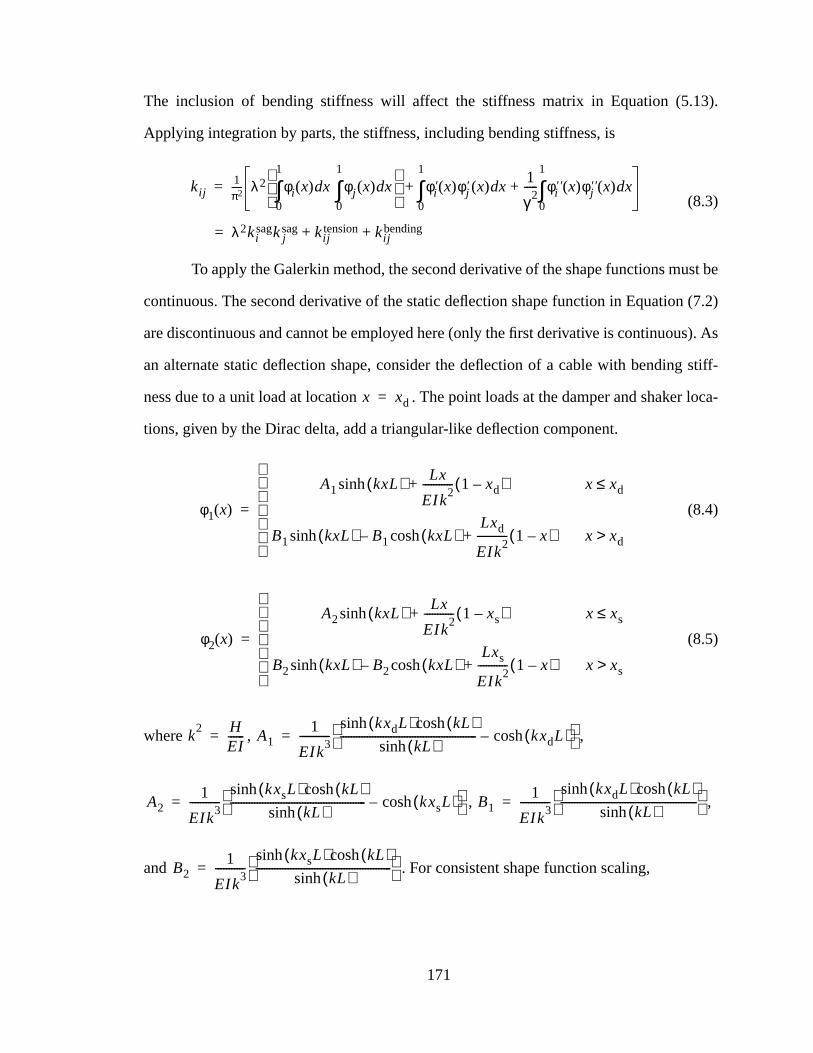
3).
st be
(7.2)
s). As
stiff-
loca-
The inclusion of bending stiffness will affect the stiffness matrix in Equation (5.1
Applying integration by parts, the stiffness, including bending stiffness, is
(8.3)
To apply the Galerkin method, the second derivative of the shape functions mu
continuous. The second derivative of the static deflection shape function in Equation
are discontinuous and cannot be employed here (only the first derivative is continuou
an alternate static deflection shape, consider the deflection of a cable with bending
ness due to a unit load at location . The point loads at the damper and shaker
tions, given by the Dirac delta, add a triangular-like deflection component.
(8.4)
(8.5)
where , ,
, ,
and . For consistent shape function scaling,
kij1π2----- λ2 φi x( ) xd
0
1
∫ φj x( ) xd0
1
∫
φi′ x( )φj
′ x( ) xd0
1
∫ 1
γ2----- φi
′′ x( )φj′′ x( ) xd
0
1
∫+ +=
λ2kisagkj
sag kijtension kij
bending+ +=
x xd=
φ1 x( )
A1 kxL( )sinhLx
EIk2
----------- 1 xd–( )+ x xd≤
B1 kxL( )sinh B1 kxL( )cosh–Lxd
EIk2
----------- 1 x–( )+ x xd>
=
φ2 x( )
A2 kxL( )sinhLx
EIk2
----------- 1 xs–( )+ x xs≤
B2 kxL( )sinh B2 kxL( )cosh–Lxs
EIk2
----------- 1 x–( )+ x xs>
=
k2 H
EI------= A1
1
EIk3
-----------kxdL( ) kL( )coshsinh
kL( )sinh--------------------------------------------------- kxdL( )cosh–
=
A21
EIk3
-----------kxsL( ) kL( )coshsinh
kL( )sinh--------------------------------------------------- kxsL( )cosh–
= B11
EIk3
-----------kxdL( ) kL( )coshsinh
kL( )sinh---------------------------------------------------
=
B21
EIk3
-----------kxsL( ) kL( )coshsinh
kL( )sinh---------------------------------------------------
=
171
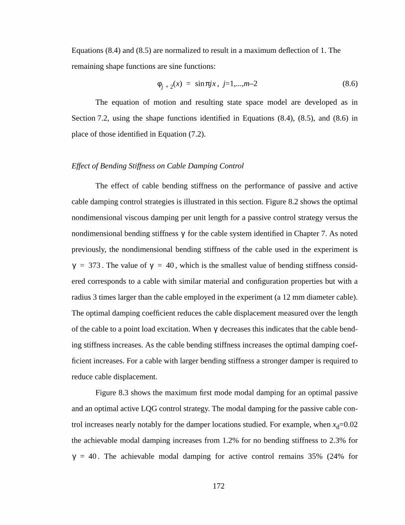
as in
6) in
ctive
timal
s the
oted
nt is
id-
ith a
able).
length
bend-
coef-
red to
sive
con-
% for
for
Equations (8.4) and (8.5) are normalized to result in a maximum deflection of 1. The
remaining shape functions are sine functions:
, j=1,...,m–2 (8.6)
The equation of motion and resulting state space model are developed
Section 7.2, using the shape functions identified in Equations (8.4), (8.5), and (8.
place of those identified in Equation (7.2).
Effect of Bending Stiffness on Cable Damping Control
The effect of cable bending stiffness on the performance of passive and a
cable damping control strategies is illustrated in this section. Figure 8.2 shows the op
nondimensional viscous damping per unit length for a passive control strategy versu
nondimensional bending stiffness for the cable system identified in Chapter 7. As n
previously, the nondimensional bending stiffness of the cable used in the experime
. The value of , which is the smallest value of bending stiffness cons
ered corresponds to a cable with similar material and configuration properties but w
radius 3 times larger than the cable employed in the experiment (a 12 mm diameter c
The optimal damping coefficient reduces the cable displacement measured over the
of the cable to a point load excitation. When decreases this indicates that the cable
ing stiffness increases. As the cable bending stiffness increases the optimal damping
ficient increases. For a cable with larger bending stiffness a stronger damper is requi
reduce cable displacement.
Figure 8.3 shows the maximum first mode modal damping for an optimal pas
and an optimal active LQG control strategy. The modal damping for the passive cable
trol increases nearly notably for the damper locations studied. For example, whenxd=0.02
the achievable modal damping increases from 1.2% for no bending stiffness to 2.3
. The achievable modal damping for active control remains 35% (24%
φj 2+ x( ) πjxsin=
γ
γ 373= γ 40=
γ
γ 40=
172
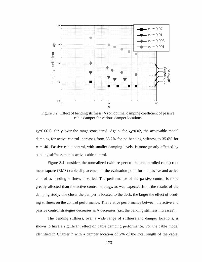
l
for
d by
root
active
more
of the
bend-
e and
s, is
odel
ble,
e
xd=0.001), for over the range considered. Again, forxd=0.02, the achievable moda
damping for active control increases from 35.2% for no bending stiffness to 35.6%
. Passive cable control, with smaller damping levels, is more greatly affecte
bending stiffness than is active cable control.
Figure 8.4 considers the normalized (with respect to the uncontrolled cable)
mean square (RMS) cable displacement at the evaluation point for the passive and
control as bending stiffness is varied. The performance of the passive control is
greatly affected than the active control strategy, as was expected from the results
damping study. The closer the damper is located to the deck, the larger the effect of
ing stiffness on the control performance. The relative performance between the activ
passive control strategies decreases as decreases (i.e., the bending stiffness increases).
The bending stiffness, over a wide range of stiffness and damper location
shown to have a significant effect on cable damping performance. For the cable m
identified in Chapter 7 with a damper location of 2% of the total length of the ca
101
102
103
102
103
104
105
106
Figure 8.2: Effect of bending stiffness ( ) on optimal damping coefficient of passivcable damper for various damper locations.
γ
xd = 0.001
xd = 0.005
xd = 0.01
xd = 0.02
γ
dam
ping
coe
ffici
ent -
c opt
no b
endi
ngst
iffne
ss
γ
γ 40=
γ
173
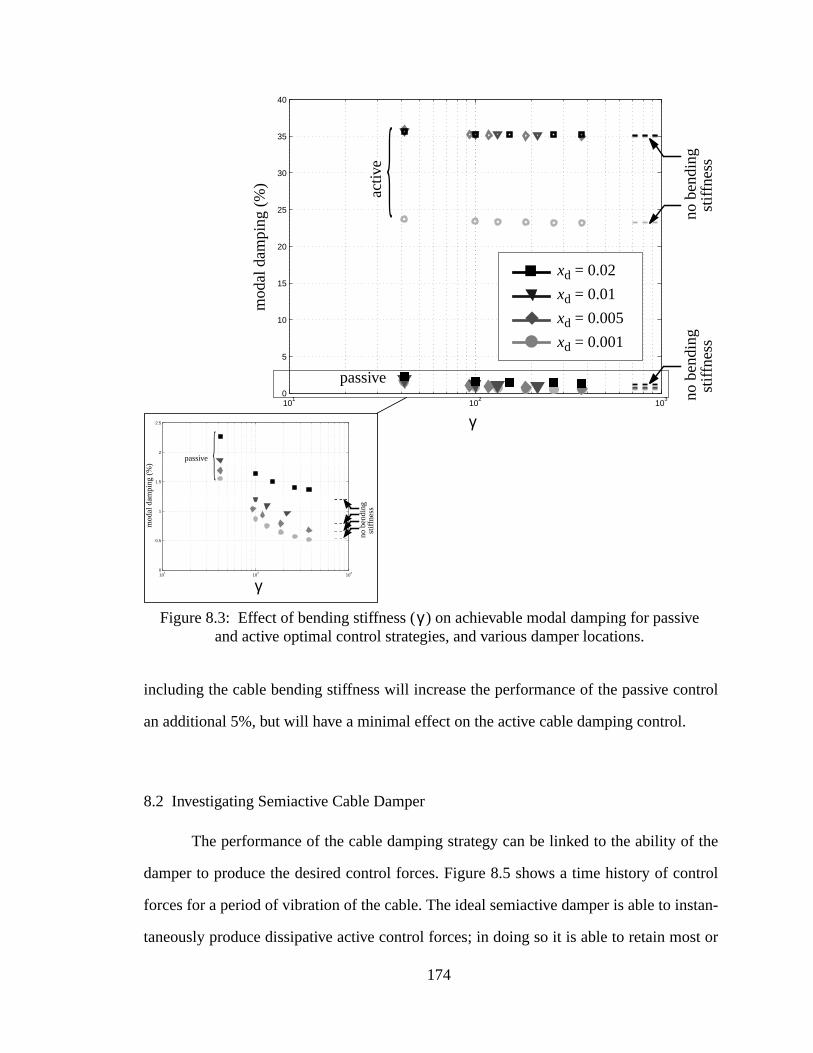
ntrol
f the
ntrol
stan-
st or
ve
including the cable bending stiffness will increase the performance of the passive co
an additional 5%, but will have a minimal effect on the active cable damping control.
8.2 Investigating Semiactive Cable Damper
The performance of the cable damping strategy can be linked to the ability o
damper to produce the desired control forces. Figure 8.5 shows a time history of co
forces for a period of vibration of the cable. The ideal semiactive damper is able to in
taneously produce dissipative active control forces; in doing so it is able to retain mo
101
102
103
0
0.5
1
1.5
2
2.5
101
102
103
0
5
10
15
20
25
30
35
40
Figure 8.3: Effect of bending stiffness ( ) on achievable modal damping for passiand active optimal control strategies, and various damper locations.
γ
xd = 0.001
xd = 0.005
xd = 0.01
xd = 0.02
γ
passiveac
tive {
no b
endi
ngst
iffne
ss
mod
al d
ampi
ng (
%)
no b
endi
ngst
iffne
ss
γ
passive{
no b
endi
ngst
iffne
ss
mod
al d
ampi
ng (
%)
174
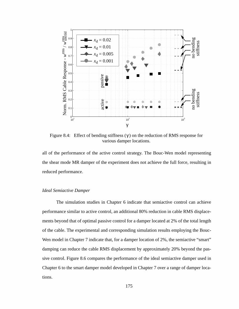
nting
ing in
ieve
ace-
ngth
ouc-
art”
e pas-
sed in
r loca-
r
all of the performance of the active control strategy. The Bouc-Wen model represe
the shear mode MR damper of the experiment does not achieve the full force, result
reduced performance.
Ideal Semiactive Damper
The simulation studies in Chapter 6 indicate that semiactive control can ach
performance similar to active control, an additional 80% reduction in cable RMS displ
ments beyond that of optimal passive control for a damper located at 2% of the total le
of the cable. The experimental and corresponding simulation results employing the B
Wen model in Chapter 7 indicate that, for a damper location of 2%, the semiactive “sm
damping can reduce the cable RMS displacement by approximately 20% beyond th
sive control. Figure 8.6 compares the performance of the ideal semiactive damper u
Chapter 6 to the smart damper model developed in Chapter 7 over a range of dampe
tions.
101
102
103
0
0.1
0.2
0.3
0.4
0.5
0.6
0.7
0.8
0.9
1
Figure 8.4: Effect of bending stiffness ( ) on the reduction of RMS response fovarious damper locations.
γ
xd = 0.001
xd = 0.005
xd = 0.01
xd = 0.02
γ
pass
ive
activ
e
Nor
m. R
MS
Cab
le R
espo
nse
-w
rms /
wrm
sun
ctld
no b
endi
ngst
iffne
ssno
ben
ding
stiff
ness
175
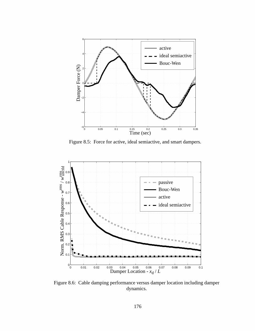
per
Figure 8.5: Force for active, ideal semiactive, and smart dampers.
0 0.05 0.1 0.15 0.2 0.25 0.3 0.35−6
−4
−2
0
2
4
6
Time (sec)
Dam
per
For
ce (
N) Bouc-Wen
ideal semiactive
active
0 0.01 0.02 0.03 0.04 0.05 0.06 0.07 0.08 0.09 0.10
0.1
0.2
0.3
0.4
0.5
0.6
0.7
0.8
0.9
1
Figure 8.6: Cable damping performance versus damper location including damdynamics.
active
Bouc-Wen
ideal semiactive
passive
Damper Location -xd / L
Nor
m. R
MS
Cab
le R
espo
nse
-w
rms /
wrm
sun
ctld
176
per
ptimal
pared
0% of
odel
ptimal
des a
% of
omes
econ-
cable
peri-
f the
ous
r is
ment
mula-
ffect
ctive
ec. For
llers.
ro-
para-
or the
udies.
At a damper location of 10% the total length of the cable, the Bouc-Wen dam
model is able to reduce RMS cable response by 23% relative to the response of the o
passive control strategy, whereas the ideal semiactive damper reduces it by 60% com
to passive control. As the damper location moves closer to the cable support, at 2-1
the total length of the cable, the relative performance of the Bouc-Wen damper m
increases slightly as it is able to reduce cable response by 25-30% compared to the o
passive control strategy. In contrast, the ideal semiactive control performance provi
reduction of up to 84%. At damper locations closer to the cable support, less than 2
the total length of the cable, the ideal semiactive control improved performance bec
even more significant, but the Bouc-Wen damper model performance deteriorates. R
ciling this difference in performance between smart damping and ideal semiactive
damping is examined in this section.
Another difference between the ideal damper system of Chapter 6 and the ex
mental and Bouc-Wen damper model strategy of Chapter 7 is the implementation o
controller. In Chapter 6 the controller is implemented in the simulation as a continu
time controller. In the experiment and simulation of Chapter 7 the digital controlle
implemented as a discrete time controller. For the digital controller used in the experi
a discrete time step of 0.005 sec was the fastest the controller was able to run. All si
tions in Chapter 7 use this time step for discretization. The discretization does not a
the performance of the Bouc-Wen model simulations. However, the ideal semia
damper performance decreases when implemented at a discrete time step of 0.005 s
this study, the ideal damper models are implemented with continuous time contro
Additionally, the simulations in Chapter 7 include a time lag for the control signal to p
duce the desired force which is neglected in the ideal damper of Chapter 6. For com
tive purposes, the performance of the damper models with the time lag is computed f
ideal semiactive damper as well as the proposed damper models in the following st
177
RMS
uous
deal
l sys-
is
gent.
ge of
amper
sults
ctive
ideal
with
is
ental
ax-
eal
hear
eal
ever,
The performance of the ideal semiactive damper is reduced from a normalized
damper displacement of 0.08 to 0.125 for the ideal damper with time lag.
Ideal Semiactive Arcrtangent Damper
The ideal semiactive system, as observed in Figure 5.3, allows for discontin
force at zero damper velocity. This discontinuity cannot be physically realized. An i
semiactive arctangent model is introduced to be more representative of the physica
tem than the ideal model. The semiactive tangent damper model is given as
(8.7)
where is the damper force of the fully active system identified in Section 5.3,
the damper velocity, and is a constant that determines the slope of the inverse tan
The performance of the ideal semiactive arctangent system is studied for a ran
values. Figure 8.7 examines the performance of the ideal semiactive arctangent d
model. This model is compared to both the experimental results and to simulation re
using Bouc-Wen damper model, ideal semiactive damper model, and ideal semia
damper model with time lag. For greater than 100 sec/m, the performance of the
semiactive arctangent system is nearly identical to the ideal semiactive damper (both
time lag). As the slope parameter is reduced, the performance degrades.
To understand the significance of this range of values of , the parameter
determined for the smart cable damper in Chapter 7. Figure 8.8 shows the experim
force versus velocity plot for the smart damper in the 12.65 m cable experiment with m
imum control signal and a sinusoidal excitation. Also on this figure is a plot of the id
semiactive arctangent damper for sec/m which is representative of the s
mode MR damper. Note, from Figure 8.7, that sec/m is sufficient for the id
arctangent damper to achieve the full performance of ideal semiactive damper. How
Fd t( )2π--- µw xd( )[ ]atan F
d
activet( ) Fd
active t( )w xd( ) 0<
0 otherwise
=
Fdactive wd
µ
µ
µ
µ
µ µ
µ 500=
µ 500=
178
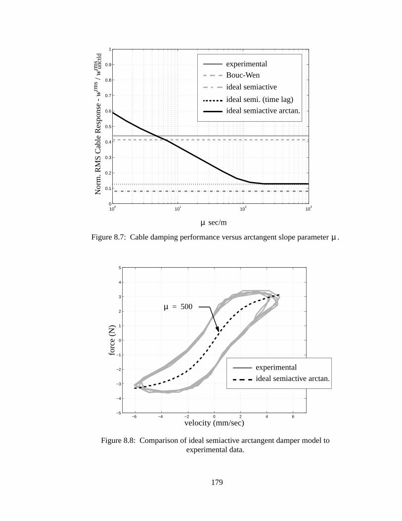
.
100
101
102
103
0
0.1
0.2
0.3
0.4
0.5
0.6
0.7
0.8
0.9
1
Figure 8.7: Cable damping performance versus arctangent slope parameterµ
ideal semiactive
Bouc-Wen
ideal semi. (time lag)
experimental
Nor
m. R
MS
Cab
le R
espo
nse
-w
rms /
wrm
sun
ctld
sec/mµ
ideal semiactive arctan.
−6 −4 −2 0 2 4 6−5
−4
−3
−2
−1
0
1
2
3
4
5
forc
e (N
)
velocity (mm/sec)
Figure 8.8: Comparison of ideal semiactive arctangent damper model toexperimental data.
ideal semiactive arctan.
experimental
µ 500=
179
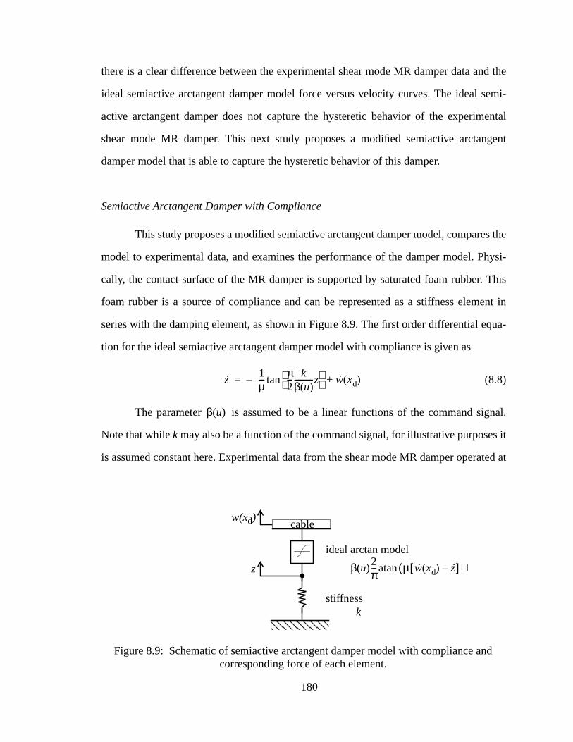
nd the
semi-
ental
ngent
es the
Physi-
. This
ent in
qua-
gnal.
s it
ated at
nd
there is a clear difference between the experimental shear mode MR damper data a
ideal semiactive arctangent damper model force versus velocity curves. The ideal
active arctangent damper does not capture the hysteretic behavior of the experim
shear mode MR damper. This next study proposes a modified semiactive arcta
damper model that is able to capture the hysteretic behavior of this damper.
Semiactive Arctangent Damper with Compliance
This study proposes a modified semiactive arctangent damper model, compar
model to experimental data, and examines the performance of the damper model.
cally, the contact surface of the MR damper is supported by saturated foam rubber
foam rubber is a source of compliance and can be represented as a stiffness elem
series with the damping element, as shown in Figure 8.9. The first order differential e
tion for the ideal semiactive arctangent damper model with compliance is given as
(8.8)
The parameter is assumed to be a linear functions of the command si
Note that whilek may also be a function of the command signal, for illustrative purpose
is assumed constant here. Experimental data from the shear mode MR damper oper
Figure 8.9: Schematic of semiactive arctangent damper model with compliance acorresponding force of each element.
stiffness
ideal arctan model
z
w(xd)
β u( )2π--- µ w xd( ) z–[ ]( )atan
k
cable
z1µ--- π
2--- k
β u( )----------z
tan– w xd( )+=
β u( )
180
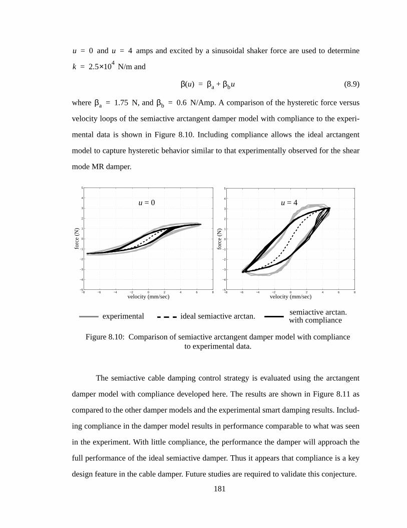
mine
us
peri-
gent
shear
ngent
.11 as
nclud-
seen
the
a key
cture.
ce
and amps and excited by a sinusoidal shaker force are used to deter
N/m and
(8.9)
where N, and N/Amp. A comparison of the hysteretic force vers
velocity loops of the semiactive arctangent damper model with compliance to the ex
mental data is shown in Figure 8.10. Including compliance allows the ideal arctan
model to capture hysteretic behavior similar to that experimentally observed for the
mode MR damper.
The semiactive cable damping control strategy is evaluated using the arcta
damper model with compliance developed here. The results are shown in Figure 8
compared to the other damper models and the experimental smart damping results. I
ing compliance in the damper model results in performance comparable to what was
in the experiment. With little compliance, the performance the damper will approach
full performance of the ideal semiactive damper. Thus it appears that compliance is
design feature in the cable damper. Future studies are required to validate this conje
u 0= u 4=
k 2.54×10=
β u( ) βa βbu+=
βa 1.75= βb 0.6=
−8 −6 −4 −2 0 2 4 6 8−5
−4
−3
−2
−1
0
1
2
3
4
5
forc
e (N
)
velocity (mm/sec)−8 −6 −4 −2 0 2 4 6 8
−5
−4
−3
−2
−1
0
1
2
3
4
5
forc
e (N
)
velocity (mm/sec)
Figure 8.10: Comparison of semiactive arctangent damper model with complianto experimental data.
semiactive arctan.experimental with complianceideal semiactive arctan.
u = 0 u = 4
181
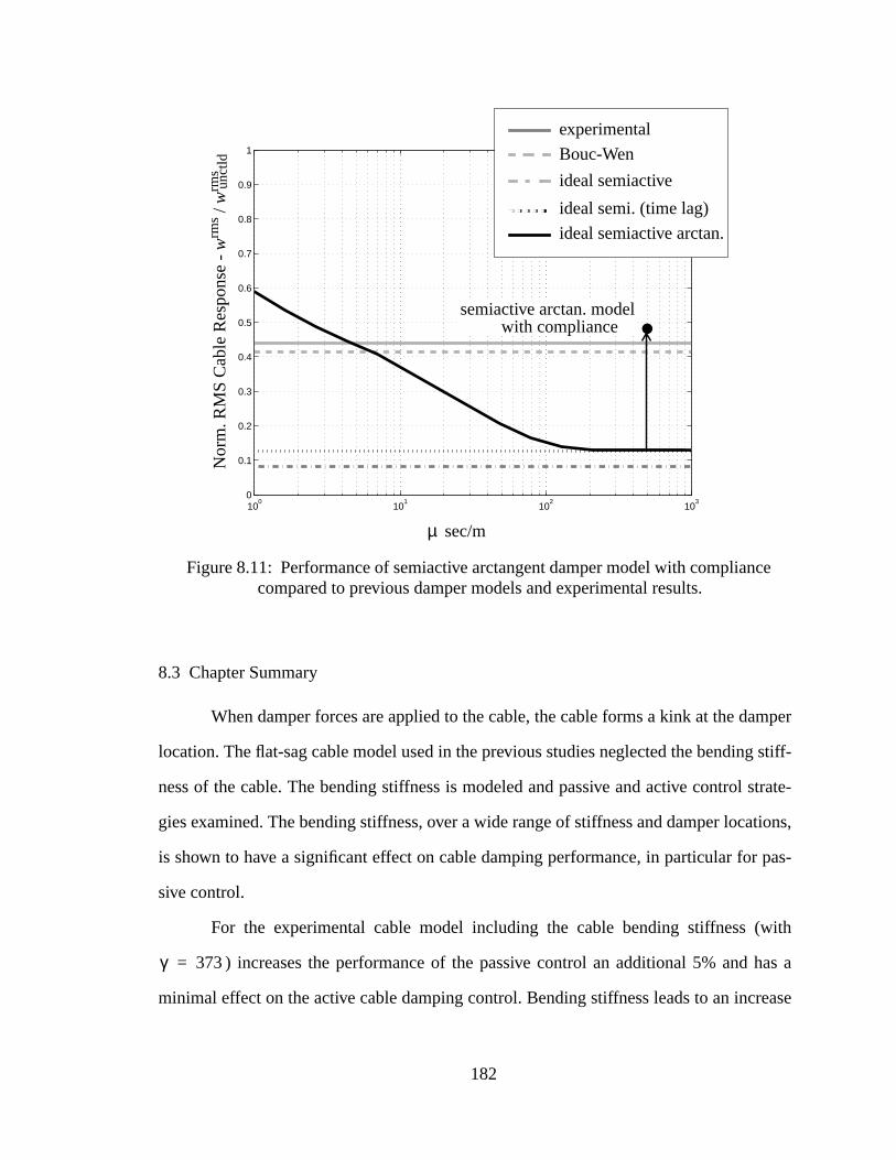
mper
g stiff-
strate-
tions,
pas-
with
has a
rease
ce
8.3 Chapter Summary
When damper forces are applied to the cable, the cable forms a kink at the da
location. The flat-sag cable model used in the previous studies neglected the bendin
ness of the cable. The bending stiffness is modeled and passive and active control
gies examined. The bending stiffness, over a wide range of stiffness and damper loca
is shown to have a significant effect on cable damping performance, in particular for
sive control.
For the experimental cable model including the cable bending stiffness (
) increases the performance of the passive control an additional 5% and
minimal effect on the active cable damping control. Bending stiffness leads to an inc
100
101
102
103
0
0.1
0.2
0.3
0.4
0.5
0.6
0.7
0.8
0.9
1
Figure 8.11: Performance of semiactive arctangent damper model with compliancompared to previous damper models and experimental results.
Nor
m. R
MS
Cab
le R
espo
nse
-w
rms /
wrm
sun
ctld
semiactive arctan. modelwith compliance
sec/mµ
ideal semiactive
Bouc-Wen
ideal semi. (time lag)
experimental
ideal semiactive arctan.
γ 373=
182

erfor-
uc-
fore,
nt in
pre-
control
force
oach
gent
smart
ideal
mper.
hieve
lica-
in cable damping performance and thus does not account for the experimental p
mance of the smart damper.
For values of on the order of 1000, as Irvine identified typical for cable str
tures, the bending stiffness has little effect for both passive and active control. There
the previous models neglecting bending stiffness are shown here to be valid.
A series of damper models are presented to identify the areas for improveme
the semiactive damper design. An ideal semiactive damper model with a time lag is
sented that is able to reduce the cable response 76% beyond that of optimal passive
for a damper location of 2% of the total length of the cable.
An ideal semiactive arctangent damper model is used to better represent the
behavior at zero velocity. The performance of this damper model is shown to appr
that of the ideal semiactive damper model. Compliance is modeled for the arctan
damper to better represent the hysteretic behavior observed experimentally in the
shear mode MR damper. The compliance is shown to reduce performance of the
semiactive arctangent damper.
It appears that damper compliance is a key design feature in the cable da
Future studies should examine and validate the level of compliance required to ac
sufficient semiactive cable damping performance in experimental and full-scale app
tions.
γ
183
zard
d the
per-
h-rise
figu-
pro-
ntrol
e per-
rimen-
tally
posed
rch,
the
duce
assive,
egies
ement
CHAPTER 9: CONCLUSIONS
This research investigated semiactive control of civil structures for natural ha
mitigation. The research has two components, the seismic protection of buildings an
mitigation of wind-induced vibration in cable structures. Analytical, numerical, and ex
imental methods are employed. The dynamic characteristics of the structures, the hig
buildings and flexible cables, are modeled and examined. The effect of structural con
rations on control performance is examined. Viable semiactive control strategies are
posed and the relative merits are compared with optimal active and passive co
strategies, which provide an upper and lower bound, respectively, on the achievabl
formance of semiactive control strategies. Control concepts are demonstrated expe
tally for both the seismically excited coupled building system and the environmen
excited cable damping system. Experimental results were presented to verify the pro
models and control strategies.
In what follows, conclusions for the two specific components of this resea
namely coupled building control and cable damping control are provided. Following
conclusions, future studies are identified.
9.1 Coupled Building Control Conclusions
Active and semiactive coupled building control strategies were proposed to re
the building responses due to seismic excitation. Previous research has identified p
active and, recently, semiactive coupled building control strategies. The control strat
presented here employ readily available absolute acceleration and relative displac
184
ntrol
ctu-
l
ffect
level
sed
den-
tural
m is
e, the
ined.
om-
MS)
yond
RMS
yond
uce
able
ween
arth-
ximum
the
rfor-
nt. In
measurements at the location of the coupling link for feedback control. The active co
strategy employsH2/LQG control, using measurements of absolute acceleration and a
ator displacement feedback. The semiactive control strategy uses clipped-optimaH2/
LQG control requiring these same feedback measurements.
A two-degree-of-freedom coupled building model is used to demonstrate the e
of coupling on the system dynamics. For passive control, it is shown that an optimal
of connector damping exists. A multi-degree-of-freedom coupled building model is u
to demonstrate the effect of building configuration on coupled building performance. I
tified are two concerns regarding the coupled building configurations. First, when na
frequencies of the coupled buildings become similar, the performance of the syste
reduced. Second, when the coupling link is located near the node of a vibratory mod
performance of the system is similarly reduced.
The efficacy of the proposed active and semiactive control strategies are exam
For buildings similar in configuration to those coupled in the Triton Square office c
plex, active control is shown to reduce the maximum absolute root mean square (R
acceleration to 65% of the uncoupled building absolute acceleration and to 20% be
that of passive control. Semiactive control is shown to reduce the maximum absolute
acceleration to 75% of the uncoupled building absolute acceleration and to 8% be
that of passive control. Limiting the maximum allowable control force is shown to red
the performance of all control strategies. As the constraint on the maximum allow
control force becomes more restrictive, the relative difference in performance bet
active, semiactive, and passive control is shown to be reduced. Also, for larger e
quakes, the buildings may be damaged and the performance objective to reduce ma
accelerations may be of less importance than reducing the interstory drift.
When the dominant coupled building natural frequencies become similar or
coupling link is located near the node of a dominant vibratory mode, the relative pe
mance difference between active and passive control is shown to be more significa
185
tion up
tally
5-ton
vel-
ctive
ons of
tem’s
build-
o sim-
tions
mic
te the
g are
es
man-
vels,
gain
sig-
trol is
l for a
semi-
these cases, active control is shown to reduce the maximum absolute RMS accelera
to 40% beyond that of passive control.
The active coupled building control proposed in this research was experimen
demonstrated using a control actuator with a ball-screw mechanism, similar to the 3
control actuators coupling the Triton Square buildings. A model of the system is de
oped for the control design that fully accounts for control-structure interaction. The a
coupled building system is shown to reduce the resonant peaks of the transfer functi
absolute story acceleration to ground acceleration to 18-67% of the uncoupled sys
resonant peaks and to 22-50% of the rigidly connected resonant peaks. The coupled
ing system is shown to reduce the maximum absolute RMS story accelerations due t
ulated ground motions to as little as 18% of the uncoupled absolute RMS accelera
and 45% of the rigidly connected system.
9.2 Cable Damping Control Conclusions
A low-order model is developed to include the effect of cable sag into the dyna
model of transverse in-plane cable vibration. The cable model is used to demonstra
effect of sag on cable damping performance. Two concerns for sag in cable dampin
identified. First, whenλ2 = (2iπ)2, symmetric and antisymmetric natural frequenci
crossover and the performance of cable damping is reduced due to an uncontrollable
ifold. Second, when the level of sag is slightly larger than the frequency crossover le
the newly formed node in the symmetric mode coincides with the damper location, a
resulting in reduced performance for the system.
Active and semiactive cable damping control is shown analytically to provide
nificantly increased performance corresponding to passive control. Semiactive con
shown to reduce cable displacement an additional 80% beyond that of passive contro
damper location at 2% the total length of the cable. These results assume an ideal
186
xpect
fluid
ilar
smart
iactive
erfor-
nge
with
has a
rease
erfor-
enti-
and
here
MR
pre-
e con-
force
oach
gent
smart
ideal
amper.
active damper and serve to provide an “upper bound” on the performance one could e
from semiactive cable damping.
Semiactive cable damping, using a shear mode magnetorheological (MR)
damper, is experimentally verified on a 12.65 m inclined cable that is dynamically sim
to a typical stay cable on a cable-stayed bridge. Combined models for the cable and
damper are established for the control design. Experimental results showed that sem
control is able to reduce the cable displacement an additional 20% beyond the p
mance of passive control.
The effect of including bending stiffness in the cable model is studied over a ra
of stiffness. The experimental cable model including the cable bending stiffness (
) increases the performance of the passive control an additional 5% and
minimal effect on the active cable damping control. Bending stiffness leads to an inc
in cable damping performance and thus does not account for the experimental p
mance of the smart damper. For values of on the order of 1000, as Irvine (1982) id
fied typical for cable structures, the bending stiffness has little effect for both passive
active control. Therefore, the previous models neglecting bending stiffness are shown
to be valid.
The difference between the ideal semiactive and experimental shear mode
damper performance is studied. An ideal semiactive damper model with a time lag is
sented that is able to reduce the cable response 76% beyond that of optimal passiv
trol. An ideal semiactive arctangent damper model is used to better represent the
behavior at zero velocity. The performance of this damper model is shown to appr
that of the ideal semiactive damper model. Compliance is modeled for the arctan
damper to better represent the hysteretic behavior observed experimentally in the
shear mode MR damper. The compliance is shown to reduce performance of the
semiactive arctangent damper and is considered a key design feature in the cable d
γ 373=
γ
187
ble
th-
ntrol
n be
ls of
, and
ive,
sym-
ace-
and
gs.
and
con-
emi-
can
to the
lex.
ol.
tive
ental
r the
ator
ed to
9.3 Future Studies
• The performance of coupled building control is limited by the maximum allowa
control force of the coupling link, particularly for larger magnitude design ear
quakes. Further studies on the detailing required to increase the maximum co
force that may be applied to a high-rise building near the top of the structure ca
examined.
• The coupled building models considered in this research are in-plane mode
two adjacent buildings. Future studies should consider in-plane, out-of-plane
torsional motion of the coupled buildings. Additionally, the performance of act
passive, and semiactive control for asymmetric building clusters as well as a
metric buildings can be examined.
• Active coupled building control using absolute acceleration and relative displ
ment measurements at the location of the coupling link is shown analytically
in a small-scale test to be an effective method of control for high-rise buildin
Experimental tests using building models to consider in-plane, out-of-plane,
torsional motion for seismic excitation can be further verified.
• The Triton Square office complex in Tokyo, Japan, was coupled using active
trol actuators earlier this year (2001). Demonstrating the active and even s
active control strategies proposed in this dissertation on full-scale applications
serve to verify the concepts proposed here as well as provide a comparison
performance of the existing system in place on the Triton Square office comp
• A clipped-optimalH2/LQG control is proposed for smart cable damping contr
This type of controller is shown to have good performance for the ideal semiac
cable damper. The particular shear-mode damper employed in the experim
studies was not able to achieve this ideal performance. The control design fo
experimental studies did not incorporate the dynamics of the combined actu
and cable in the control design process. Future studies should be pursu
188

ture
p to
ping
men-
d to
d for
develop new control algorithms, possibly nonlinear control strategies, to cap
the dynamics of the MR damper.
• Identifying the damper characteristics that limit overall performance can hel
develop smart dampers to provide for increased performance in cable dam
applications. In particular, compliance appears in this research to have a detri
tal effect on cable damping performance. The level of compliance require
achieve sufficient semiactive cable damping performance needs to be verifie
experimental and full-scale applications.
189
the
xcita-
auss-
ill also
n sto-
utput
m per-
state
lace-
ystem
square
and
APPENDIX A: ROOT MEAN SQUARE RESPONSES OF A FIRST ORDER LINEAR
SYSTEM USING THE SOLUTION TO THE LYAPUNOV EQUATION
The ground excitation for the coupled building system in Chapters 2-4 and
cable excitation for the smart cable damping system in Chapters 5-8 are random e
tions. These excitations are modeled in this work as filtered zero-mean stationary G
ian white noise processes. Since the excitation is a stochastic process, the output w
be a stochastic process. In fact, since the system is linear, it will also be a Gaussia
chastic process, fully defined by the mean vector and covariance. The mean of the o
is zero. Thus the root mean square (RMS) response is a good measure of the syste
formance. This appendix outlines the process of determining RMS responses of a
space system of equations (Soong and Grigoriu, 1993).
The covariance of the state vector of the first order linear state space system
(A.1)
can be written as
(A.2)
where is the expected value and is the mean of the state vector. The disp
ments and velocities of the buildings have a zero mean. Therefore, the states of the s
are all zero mean processes ( ), and the covariance reduces to the mean
value of the state
(A.3)
Taking the time derivative of the covariance, as defined in Equation (A.3),
applying the chain rule to the right hand side results in
z t( ) Az t( ) Bw t( )+=
Gzz E zzT mzmzT
–[ ]=
E .[ ] mz
mz 0=
Gzz t( ) E z t( )zTt( )[ ]=
190
the
)
ua-
) is
some
time.
,
(A.7)
as
)
(A.4)
Equation (A.4) can be expanded using the state equation to
(A.5)
The cross-correlation terms and are now determined realizing that
response can be formulated as the following integral of (and assuming
(A.6)
The cross-correlation function can be written using the relationship in Eq
tion (A.6) as
(A.7)
The expected value of the first integral on the right hand side of Equation (A.7
equal to zero by the argument that the response is independent of the excitation
for (the system is causal). This equality can be understood as the excitation at
time in the future, or even at the exact instant, will not affect the state at the present
Also recall that and . Over the interval of the integral,
the expected value of the state and the excitation can be written as
(A.8)
The expected value of the second integral on the right hand side of Equation
can be rewritten, using the covariance matrix of the white noise defined
, as
(A.9)
Taking into account the value of the integral in Equation (A.9) (recall that
(A.10)
Gzz t( ) E zzT zzT+[ ]=
Gzz AGzz GzzAT BGwz GzwBT
+ + +=
Gwz Gzw
z t( ) z t0( ) 0=
z t( ) z u( ) udt0
t∫ Az u( ) Bw u( )+( ) udt0
t∫ Az u( ) udt0
t∫ Bw u( ) udt0
t∫+= = =
Gzw
Gzw t( ) E z t( )w t( )[ ] E Az u( )w t( ) udt0
t∫ Bw u( )wTt( ) ud
t0
t∫+[ ]= =
z u( ) w t( )
u t≤
E w t( )[ ] 0= E z u( )[ ] 0= u t≤
E Az u( )w t( ) udt0
t∫[ ] A E z u( )w t( )[ ] udt0
t∫ A E z u( )[ ]E w t( )[ ] udt0
t∫ 0= = =
E w u( )wTt( )[ ] 2πSoδ u t–( )≡
E Bw u( )wTt( ) ud
t0
t∫[ ] B E w u( )wTt( )[ ] ud
t0
t∫ 2πBSo δ u t–( ) udt0
t∫= =
u t≤
δ u t–( ) udt0
t∫ 0.5=
191
ons
in-
then
state,
s, the
The cross-correlation function of Equation (A.7) can be written using Equati
(A.7) through (A.9) as
(A.11)
Additionally, it can be shown that
(A.12)
Substituting Equations (A.10), (A.11) and (A.12) into Equation (A.5) and comb
ing terms results in the following
(A.13)
Assuming the vectorz is a stationary process (the transient effects have died out),
and Equation (A.13) takes the form
(A.14)
which is in the form of a Lyapunov equation that can be solved in MATLAB using the func-
tion lyap to determine the value of , the covariance matrix of the state vector .
The covariance of the output can be determined from the covariance of the
where , as
(A.15)
The RMS responses are the square root of the covariance of the response
diagonal terms of determined as
(A.16)
Gzw t( ) 0 2πBSo 0.5( )+ πBSo= =
Gwz t( ) πSoBT=
Gzz AGzz GzzAT
2πBSoBT+ +=
Gzz 0=
AGzz GzzAT
2πBSoBT+ + 0=
Gzz z
ye Cz=
GyeyeE yeye
T[ ] E Cz Cz( )T[ ] E CzzTCT[ ] CE zzT[ ]CT CGzzCT
= = = = =
Gyeye
yerms
diag Gyeye( )=
192
The
erkin
an-
).
epre-
an
are
APPENDIX B: MODELING TALL ADJACENT BUILDINGS USING THE
GALERKIN METHOD
The Galerkin method is employed to model the coupled building system.
equations of motion for the coupled building system are determined using the Gal
method.
The in-plane motion for thekth building, subjected to ground acceleration
and the coupling force , is given by the equation of motion for a uniform flexural c
tilevered beam with mass proportional viscous damping (Clough and Penzien, 1993
(B.1)
Applying the Galerkin method, the response of the system is assumed to be r
sented by the finite series
(B.2)
where is the horizontal displacement of thekth building, is theith trial function of
thekth building is theith generalized coordinate of thekth building andn is sufficiently
large.
The trial functions, , are taken as the closed-form eigenfunctions of
Euler-Bernoulli fixed-free beam (cantilever beam). The closed-form eigenfunctions
determined as follows.
xg t( )
f t( )
mk
∂2xk y t,( )
∂t2
----------------------- ck
∂xk y t,( )∂t
--------------------- EIk
∂4xk y t,( )
∂x4
-----------------------+ + mkxg– δ x hc–( ) f t( )∑–=
xk y t,( ) fki
y( )qki
t( )i 1=
n
∑ fkT
y( )qk t( )= =
xk fki
qki
fki
y( )
193
the
ing
it
f the
at
and
ting
ions
con-
is
.5),
not
ng the
Using simple beam theory, the 4th-order partial differential equation governing
flexural vibration of an undamped uniform Euler-Bernoulli beam with no external forc
function (Meirovitch, 1986) is
(B.3)
whereE is the modulus of elasticity,I is the moment of inertia, is the mass per un
length of the beam, and is the lateral response of the building as a function o
height,y, and time,t. The solution of this problem requires two boundary conditions
each end of the beam.
Each building, modeled as a cantilever beam, is fixed at the ground ( )
free at the roof ( ). This results in two geometric boundary conditions (resul
from the system geometry) from the fixed end and two natural boundary condit
(resulting from the force and moment equilibrium) from the free end. The boundary
ditions are
,
, (B.4)
where the notation is employed.
Using separation of variables, a solution of the form
sought. The general solution ofT(t) is
(B.5)
and is periodic with a frequency of . To determine the two constants of Equation (B
initial conditions for the displacement and velocity are required. For this study, it is
necessary to determine these particular constants, as the focus will be on determini
eigenfunction of the system to be used as a trial function in the Galerkin method.
The solution of takes the form
(B.6)
EI–y
4
4
∂∂
x y t,( ) mt2
2
∂∂
x y t,( )=
m
x y t,( )
y 0=
y L=
x 0 t,( ) 0= xyy L t,( ) 0=
xy 0 t,( ) 0= xyyy L t,( ) 0=
xy y t,( )y∂
∂x y t,( )=
x y t,( ) f y( )T t( )=
T t( ) C1 ωt C2 ωtcos+sin=
ω
f y( )
f y( ) C3 by C4 bysinh+ C5 by C6 bycosh+cos+sin=
194
our
om
ant
ated
sys-
from
d
cou-
gonal-
where . Using the four boundary conditions of Equation (B.4), three of the f
constantsC3-C6 can be determined. The values for are solved for numerically fr
the equation
(B.7)
An approximation of the above equation, providing accuracy to four signific
digits for is given as
(B.8)
The first five solutions are =[1.8751, 4.6941, 7.8548, 10.996, 14.137]T, where
the first three terms are found using Equation (B.7) and terms four and five are estim
from Equation (B.8). Once we have solved for the natural frequencies, , of the
tem are found as
(B.9)
The eigenfunctions of the system described in Equation (B.3) are determined
the boundary conditions as
(B.10)
where the constant , is a product of the unsolved constant ofC3-C6 and can be set to any
value to produce a desired norm (e.g., ). At this point, closed form solu-
tions for the mode shapes of cantilevered beams are known, Equation (B.10).
Substituting Equation (B.2) into Equation (B.1), premultiplying by , an
integrating over the height of the building, the combined equations of motion for the
pled building system are
(B.11)
where the mass, damping and stiffness matrices are diagonal as a result of the ortho
ity of the trial functions, and all of the matrices are defined as
b4 ω2
mEI
-----------=
biL
biL biLcoshcos 1–=
i 3>
biLπ2--- 2i 1–( )≅
bL
bL ωi
ωi biL( )2 EI
L4m
----------=
fiy( ) ai biL biLsinh–sin( ) bi y bi ysinh–sin( )
biL biLcosh+cos( ) bi y bi ycosh–cos( )+
[]
=
ai
mfk y( )2yd
0
L
∫ 1=
fkT
y( )
Mq t( ) Cq t( ) Kq t( )+ + G xg t( )– P f t( )+=
195
l
r by
ency,
, , , , , and
, where , ,
, and , and where the moda
damping for each building is determined as follows.
The undamped natural frequencies are found either from Equation (B.9), o
solving the eigenvalue problem
(B.12)
where .
The modal damping matrix for thekth building is then
(B.13)
where and are the model damping ratio and the undamped natural frequ
respectively, for theith mode of thekth building, and the damping matrix for thekth build-
ing is
. (B.14)
MM 1 0
0 M2
= CC1 0
0 C2
= KK1 0
0 K2
= GG1
G2
= PP1
P2
=
q t( )q1 t( )
q2 t( )= M k mk fk
Ty( )fk y( ) yd
0
hk
∫= Gk mk fkT
y( ) yd
0
hk
∫=
Pk fk hc( )= K k EI( )kx
2
2
∂∂ fk
Ty( )
x2
2
∂∂ fk y( )
yd
0
hk
∫=
Ck
M kΛk2 K k+( )Fk 0=
Λk diag ω1k ω2
k ... ωnk
=
Ck
2ζ1 k, ω1 k, 0 0 0
0 2ζ2 k, ω2 k, 0 0
0 0 ... 0
0 0 0 2ζn k, ωn k,
=
ζi k, ωi k,
Ck M kFkCkFk1–
=
196
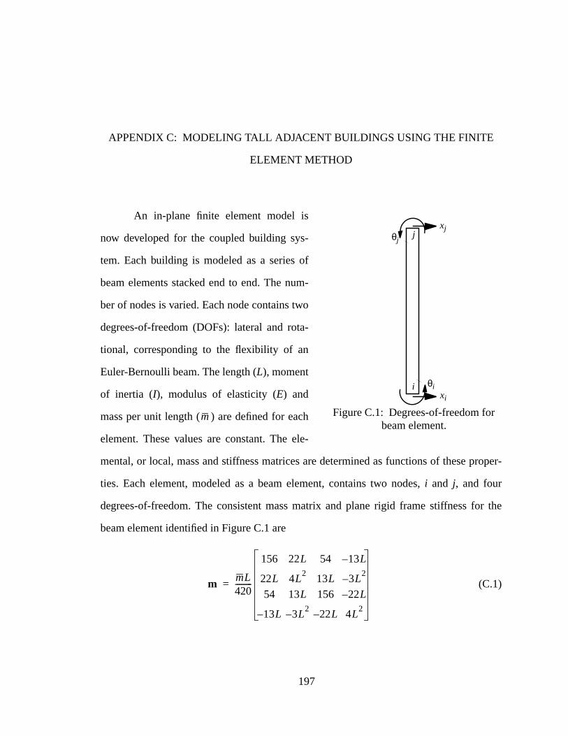
roper-
r the
APPENDIX C: MODELING TALL ADJACENT BUILDINGS USING THE FINITE
ELEMENT METHOD
An in-plane finite element model is
now developed for the coupled building sys-
tem. Each building is modeled as a series of
beam elements stacked end to end. The num-
ber of nodes is varied. Each node contains two
degrees-of-freedom (DOFs): lateral and rota-
tional, corresponding to the flexibility of an
Euler-Bernoulli beam. The length (L), moment
of inertia (I), modulus of elasticity (E) and
mass per unit length ( ) are defined for each
element. These values are constant. The ele-
mental, or local, mass and stiffness matrices are determined as functions of these p
ties. Each element, modeled as a beam element, contains two nodes,i and j, and four
degrees-of-freedom. The consistent mass matrix and plane rigid frame stiffness fo
beam element identified in Figure C.1 are
(C.1)
xi
xj
θi
θj
i
j
Figure C.1: Degrees-of-freedom forbeam element.
m
mmL420---------
156 22L 54 13L–
22L 4L2
13L 3L2
–
54 13L 156 22L–
13L– 3L2
– 22L– 4L2
=
197
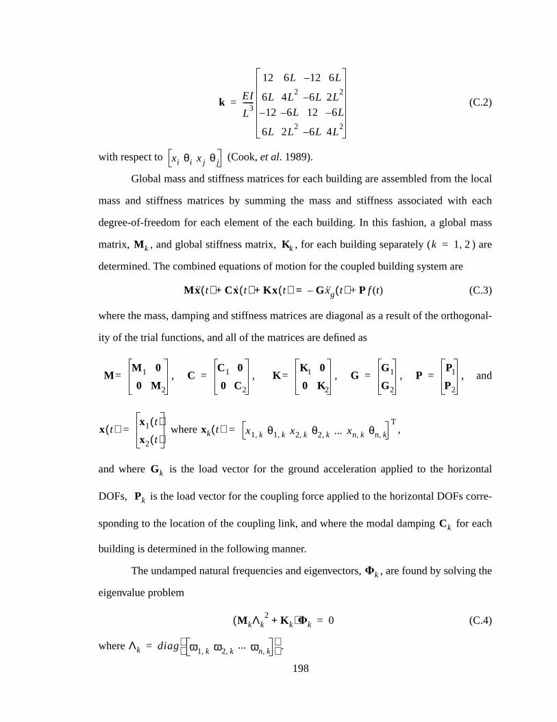
local
each
mass
are
gonal-
ntal
rre-
ach
g the
(C.2)
with respect to (Cook,et al. 1989).
Global mass and stiffness matrices for each building are assembled from the
mass and stiffness matrices by summing the mass and stiffness associated with
degree-of-freedom for each element of the each building. In this fashion, a global
matrix, , and global stiffness matrix, , for each building separately ( )
determined. The combined equations of motion for the coupled building system are
(C.3)
where the mass, damping and stiffness matrices are diagonal as a result of the ortho
ity of the trial functions, and all of the matrices are defined as
, , , , , and
where ,
and where is the load vector for the ground acceleration applied to the horizo
DOFs, is the load vector for the coupling force applied to the horizontal DOFs co
sponding to the location of the coupling link, and where the modal damping for e
building is determined in the following manner.
The undamped natural frequencies and eigenvectors, , are found by solvin
eigenvalue problem
(C.4)
where .
kEI
L3
------
12 6L 12– 6L
6L 4L2
6L– 2L2
12– 6L– 12 6L–
6L 2L2
6L– 4L2
=
xi θi x j θ j
M k Kk k 1 2,=
Mx t( ) Cx t( ) Kx t( )+ + G xg t( )– P f t( )+=
MM 1 0
0 M2
= CC1 0
0 C2
= KK1 0
0 K2
= GG1
G2
= PP1
P2
=
x t( )x1 t( )
x2 t( )= xk t( ) x1 k, θ1 k, x2 k, θ2 k, ... xn k, θn k,
T=
Gk
Pk
Ck
Fk
M kΛk2 K k+( )Fk 0=
Λk diag ω1 k, ω2 k, ... ωn k, =
198
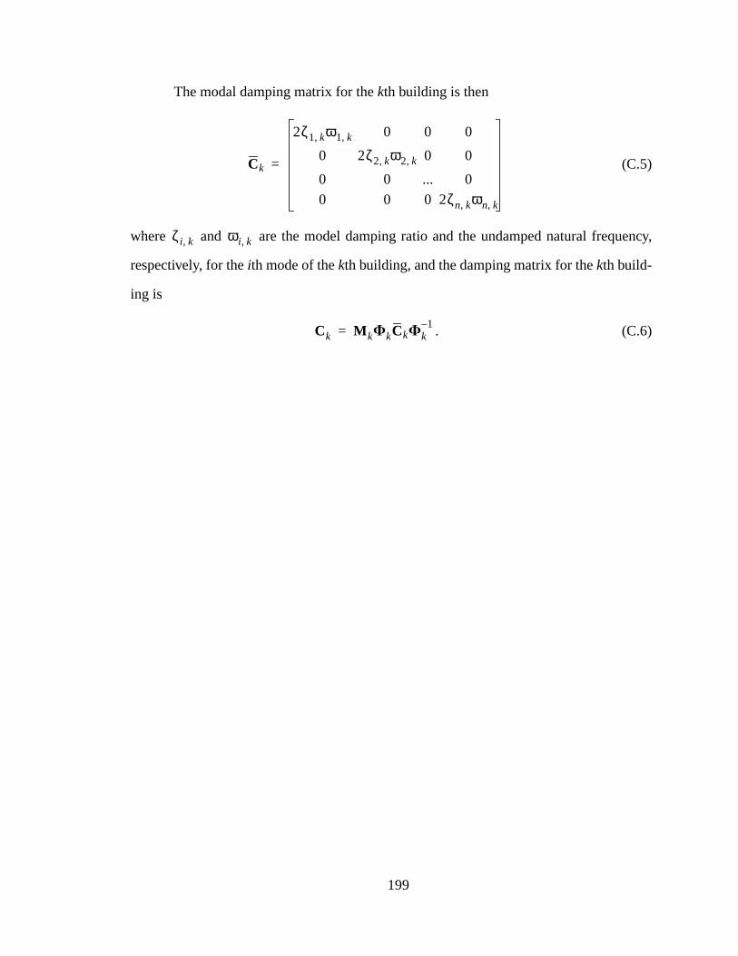
ency,
The modal damping matrix for thekth building is then
(C.5)
where and are the model damping ratio and the undamped natural frequ
respectively, for theith mode of thekth building, and the damping matrix for thekth build-
ing is
. (C.6)
Ck
2ζ1 k, ω1 k, 0 0 0
0 2ζ2 k, ω2 k, 0 0
0 0 ... 0
0 0 0 2ζn k, ωn k,
=
ζi k, ωi k,
Ck M kFkCkFk1–
=
199
andr-
ame.
truc-
e-
the
Don-ch-
BIBLIOGRAPHY
1994 Uniform Building Code, (1994), Chap. 16, Div. III, Section 1628
Baker, G.A., Johnson, E.A., Spencer, B.F., Jr., and Fujino, Y. (1999a), ModelingSemiactive Damping of Stay Cables,13th ASCE Engineering Mechanics Division Confeence, Johns Hopkins University, Baltimore, Maryland, June 13-16, 1999.
Baker, G.A. (1999b).Modeling and Semiactive Damping of Stay Cables. Master’s The-sis, Department of Civil Engineering and Geological Sciences, University of Notre D
Battaini, M., Yang, G., and Spencer, B.F., Jr. (2000), Bench-Scale Experiment for Stural Control,Journal of Engineering Mechanics, ASCE,126(2), 140-148.
Bendat, J.S., and Piersol, A.G. (1986),Random Data Analysis and Measurement Procdures, 2nd Edition, John Wiley & Sons, New York.
Burton, S.A., Makris, N., Konstantopoulos, I., and Antsaklis, P.J. (1996), Modelingresponse of ER damper: phenomenology and emulation,Journal of Engineering Mechan-ics, ASCE,122, 897-906.
Carlson, J.D. (1994), The Promise of Controllable Fluids,Proc. of Actuator 94(H. Borg-mann and K. Lenz, Eds.), AXON Technologie Consult GmbH, 266-270.
Chen, J.C. (1984), Response of Large Space Structures with Stiffness Control,Journal ofSpacecraft Rockets, 21(5), 463-467.
Chen, Y. (2000), Size Design of Viscous Damper Connected with Cable, Report No.ting Bridge - 1, Department of Civil & Structural Engineering, The Hong Kong Polytenic University, August 2000.
200
art’
ontrol
ontrolia
erifi-e
ation-
mpingtruc-
ion,
xperi-res,
Christenson, R.E., and Spencer Jr., B.F. (1999a), Coupled Building Control Using ‘SmDampers,Proc. 13th ASCE Engineering Mechanics Division Conference, Baltimore,Maryland, CD-ROM (6 pages), June 13-16, 1999.
Christenson, R.E., Spencer Jr., B.F., and Johnson, E.A. (1999b), Coupled Building Cusing Active and Smart Damping Strategies, B.H.V. Topping and B. Kumar (eds.),Opti-mization and Control in Civil and Structural Engineering, Civil-Comp Press, 187-195.
Christenson, R.E., Spencer Jr., B.F., and Johnson, E.A. (2000a), Coupled Building Cusing ‘Smart’ Damping Strategies,Proc. SPIE Smart Structures and NDE Sympos,Newport Beach, CA, CD-ROM (9 pages), March 6-9, 2000.
Christenson, R.E., Spencer Jr., B.F., Hori, N., and Seto, K. (2000b), Experimental Vcation of Coupled Building Control,Fourteenth Engineering Mechanics Conferenc,American Society of Civil Engineers, Austin, Texas, May 21-24, 2000.
Christenson, R.E., B.F. Spencer Jr., and E.A. Johnson (2001a), Experimental Verificof Semiactive Damping of Stay Cables,Proceedings of the 2001 American Control Conference, Arlington, Virginia, 5058-5063, June 25-27, 2001.
Christenson, R.E., E.A. Johnson, and B.F. Spencer Jr. (2001b), Smart Stay Cable DaExperiment,2001 Mechanics and Materials Summer Conference, Symposium on Stural Contol, Identification, and Monitoring, San Diego, California, June 27-29, 2001.
Clough, R.W., and Penzien, J. (1993),Dynamics of Structures, McGraw Hill, New York.
Cook, R., Malkus, D.S., and Plesha, M.E. (1989),Concepts and Applications of FiniteElement Analysis, John Wiley & Sons, New York.
Dowdell, D.J., and Cherry, S. (1994), Structural Control Using Semi-Active FrictDampers, Proc. 1st World Conf. on Struct. Control, Pasadena, California, FA1:59-68August 1994.
Dyke, S.J. Spencer Jr., B.F., Quast, P., Sain, M.K., and Kaspari Jr., D.C. (1994a), Emental Verification of Acceleration Feedback Control Strategies for MDOF StructuProc. of the 2nd Int. Conf. on Comp. Mech., Athens, Greece, June 13-15.
201

xperi-don
truc-
ntrol
ple-
ponse
study
entss
eo-
ngita
re,
Dyke, S.J., Spencer Jr., B.F., Quast, P., Kaspari Jr., D.C., and Sain, M.K. (1994b), Emental Verification of Acceleration Feedback Control Strategies for an Active TenSystem, NCEER Technical Report NCEER-94-024.
Dyke, S.J., Spencer Jr., B.F., Quast, P., and Sain, M.K. (1995), The Role of Control-Sture Interaction in Protective System Design,Journal of Engineering Mechanics,ASCE,121(2), 322-338.
Dyke, S.J., B.F. Spencer, Jr., M.K. Sain, and J.D. Carlson (1996a), Modeling and Coof Magnetorheological Dampers for Seismic Response Reduction.Smart Materials andStruct., 5, 565–575.
Dyke, S.J., Spencer Jr., B.F., Quast, P., Kaspari Jr., D.C., and Sain, M.K. (1996b), Immentation of an Active Mass Driver Using Acceleration Feedback Control,Microcomput-ers in Civil Engineering: Special Issue on Active and Hybrid Structural Control, 11, 304-323.
Dyke, S.J., Spencer, B.F., Jr., Sain, M.K., and Carlson, J.D. (1996c), Seismic ResReduction Using Magnetorheological Dampers,Proc. IFAC World Congress, San Fran-cisco, CA, L, 145-150, June 30-July 5, 1996.
Dyke, S.J., Spencer Jr., B.F., Sain, M.K., and Carlson, J.D. (1998), An experimentalof MR dampers for seismic protection,Smart. Mat., and Struct., 5, 693-703.
Edwards, A.T., and Boyd, J.M. (1965), Bundle-Conductor-Spacer Design Requiremand Development of ‘Spacer-Vibration Damper’,IEEE Transactions on Power Apparatuand Systems, PAS-84(10), 924–932.
Ehrgott, R.C., and Masri, S.F. (1994), Structural Control Applications of an Electrorhlogical Device, Proc. Int. Workshop on Struct. Control, USC Publication Number CE-9311, 115-129.
Endo, T., Iijima, T., Okukawa, A., and Ito, M. (1991), The Technical Challenge of a LoCable-Stayed Bridge — Tatara Bridge, In M. Ito, Y. Fujino, T. Miyata, and N. Nar(eds.),Cable-stayed Bridges — Recent Developments and their Future, Elsevier, 417–436.
Ezure, K., Kamozaki, H., and Seto, K. (1993), Vibration Control of Flexible StructuJournal of JSME, No. 930-8, 55-58. (in Japanese)
202

ble
mart-
ble
In-l
on,
ns-
trol
art 1:
art 2:
,
ystem
Ezure, K., Mitsuta, S., and Seto, K. (1994), Modeling and Vibration Control of FlexiStructures Arranged in Parallel,Journal of JSME, 60-571C, 781. (in Japanese)
Fu, Y., Dyke, S.J., and Caicedo, J.M. (1999), Seismic Response Control Using SDampers,Proc. of the 1999 American Control Conference, San Diego, California, June 24, 1999.
Fujino, Y., Warnitchai, P., and Pacheco, B.M. (1993), Active Stiffness Control of CaVibration,Trans. of ASME, 60, 948-953.
Fujino, Y., and Susumpow, T. (1994), An Experimental Study on Active Control ofplane Cable Vibration by Axial Support Motion,Earthquake Engineering and StructuraDynamics, 23, 1283-1297.
Fujino, Y., and Susumpow, T. (1995), Active Control of Cables by Axial Support MotiSmart Mater. Struct.4, A41-A51.
Fujino, Y., and Yoshida, Y. (2001), Wind-Induced Vibration and Control of the TraTokyo Bay Crossing Bridge,Journal of Structural Engineering, ASCE, accepted.
Fukuda, Y. Matsumoto, Y., and Seto, K. (1996), Bending and Torsional Vibration Conof Flexible Structures Arranged in Parallel,Proc. Third International Conference onMotion and Vibration Control (MOVIC), Chiba, Japan,3, 12-17, September 1996.
Gavin, H.P., Hanson, R.D., and Filisko, F.E. (1996a), Electrorheological dampers, panalysis and design,J. Applied Mech., ASME,63, 669-675.
Gavin, H.P., Hanson, R.D., and Filisko, F.E. (1996b), Electrorheological dampers, ptesting and modeling,J. Applied Mech., ASME,63, 676-682.
Gimsing, N.J. (1983). Cable-Supported Bridges, John Wiley & Sons, ChichesterEngland.
Ginsberg, J.H., and Pham, H. (1995), Forced Harmonic Response of a Continuous sDisplaying Eigenvalue Veering Phenomena,Journal of Vibration and Acoustics, 117(4),439-444.
203
lingT.P.
leC
on
on-
truc-
truc-
asri,l Con-
Size
m of
Graham, M.C. (1994),Design Strategies for Coupling Buildings, Master’s Thesis at theMassachusetts Institute of Technology.
Gurley, K., Kareem, A., Bergman, L.A., Johnson, E.A., and Klein, R.E. (1994), Couptall buildings for control of response to wind, in G.I. Schueller, M. Shinozuka, and J.Yao (eds.)Structural Safety & Reliability, Balkema, Rotterdam, 1553-1560
Hagedorn, P. (1988), Active Vibration Damping in Large Flexible Structures,Proc. 17thInt. Congr. Theor. Appl. Mech., Grenoble, France, 83-100 , August 21-27, 1988.
Haramoto, H., Seto, K., and Koike, Y. (1999), Active Vibration Control of Triple FlexibStructures Arranged in Parallel,Proc. of Pioneering International Symposium on MOVIin Mechantronics, Tokyo, Japan, April 1999.
Hori, N., and Seto, K. (1999), Vibration Control of Flexible Space Structures BasedReduced Order Model Method and Filtered LQ Control Theory,Proc. Pioneering Interna-tional Symposium on MOVIC in Mechantronics, Tokyo, Japan, 187-192, April 1999.
Hori, N., Christenson, R.E., Seto, K., and Spencer, B.F., Jr. (2000), Active Vibration Ctrol of Coupled Buildings Using Relative Movement,Proc. of the Fifth Motion and Vibra-tion Conference, Sydney, Australia, December 2000 (6 pages).
Housner, G.W., Soong, T.T., and Masri, S.F. (1994a), Second Generation of Active Stural Control in Civil Engineering,Proc. 1st World Conf. on Struct. Control, Pasadena,California, Panel:3-18, August 1994.
Housner, G.W., Soong, T.T., and Masri, S.F. (1994b), Second Generation of Active Stural Control in Civil Engineering,Microcomputers in Civil Engineering, 11 (5), 289-296.
Housner, G.W., Bergman, L.A., Caughey, T.K., Chassiakos, A.G., Claus, R.O., MS.F., Skelton, R.E., Soong, T.T., Spencer, B.F., Jr., and Yao, J.T.P. (1997), Structuratrol: Past and Present,Journal of Engineering Mechanics, ASCE,123(9), 897–971.
Iemura, H., Igarashi, A., and Inoue, Y. (1998), Dynamic Response Control of RealStructural Systems with Active Mass and Joint Dampers.
Ikawa, N., Yamada, Y., Yokyama, H., and Tachibana, E. (1996), Active Control SysteCoupled Structures with a Negative Stiffness,Journal of JSME(B), 42, 629-634. (in Japa-nese)
204
egy,
of
uc-
com-
Stay
23.
Stay:f
amp-
ing ofm-
Damp-f
ing of
Inaudi, J.A. (1997), Modulated Homogeneous Friction: A Semi-Active Damping StratEarthquake Engrg., and Struct. Dyn., 26, 361-376.
Irvine, H.M. (1981).Cable Structures, MIT Press, Cambridge, Massachusetts.
Iwanami, K., Suzuki, K., and Seto, K. (1986), Studies of the Vibration Control MethodParallel Structures (The Method by the Theory of P, T, Q),Journal of JSME(A), No. 86-0247, 3063-3072. (in Japanese).
Iwanami, K., Suzuki, K., and Seto, K. (1993), Vibration Control Method of Parallel Strtures Connected to Each Other with Damper and Spring,Journal of JSME(C), No. 93-0355, 69-74. (in Japanese)
Jansen, L.M., and Dyke, S.J. (2000), Semiactive control strategies for MR dampers:parative study,J. Engrg. Mech.,ASCE126(8), 795-803.
Johnson, E.A., Spencer, B.F., Jr., and Fujino, Y. (1999), Semiactive Damping ofCables: A Preliminary Study,Proceedings of the 17th International Modal Analysis Con-ference (IMAC XVII), Society for Experimental Mechanics, Bethel, Connecticut, 417–4
Johnson, E.A., Baker, G.A., Spencer, B.F., Jr., and Fujino, Y. (2000a), MitigatingCable Oscillation using Semiactive Damping,Smart Structures and Materials 2000Smart Systems for Bridges, Structures, and Highways(S.C. Liu, ed.), Proceedings oSPIE,3988, 207–216, March 6-9, 2000, .
Johnson, E.A., Baker, G.A., Spencer, B.F., Jr., and Fujino, Y. (2000b), Semiactive Ding of Stay Cables,Journal of Engineering Mechanics, ASCE, accepted.
Johnson, E.A., Christenson, R.E., and Spencer, B.F., Jr. (2000c), Semiactive DampCables with Sag,Proc. of the International Conference on Advances in Structural Dynaics, Hong Kong, China, 327-334, December 2000.
Johnson, E.A., Christenson, R.E., and Spencer, B.F., Jr. (2001a), Smart Stay Cableing - Effects of Sag and Inclination,Structural Safety and Reliability: Proceeding oICOSSAR ‘01, the 8th International Conference on Structural Safety and Reliability, New-port Beach, California, June 2001 (8 pages).
Johnson, E.A., Christenson, R.E., and Spencer, B.F., Jr. (2001b), Semiactive DampCables with Sag,Computer Aided Civil and Infrastructure Engineering, in review.
205

temi-
for
indt-
ns
-17,
ou-
mic
rch ,
portTech-
Kageyama, M., Yohida, O., and Yasui, Y. (1994), A Study on Optimal Damping Sysfor Connected Double Frame Structures,Obayashi Corporation Technical Research Insttute, 1855-1860. (in Japanese)
Kamagata, K. Miyajima K., and Seto, K. (1996), Optimal Design of Damping DevicesVibration Control of Parallel Structures,Proc. Third International Conference on Motionand Vibration Control (MOVIC), Chiba, Japan,2, 334-339, September 1996.
Kareem, A. (1994), The Next Generation of Tuned Liquid Dampers,Proc. 1st WorldConf. on Struct. Control, Pasadena, California, FP3:19-28, August 1994.
Klein, R.E., Cusano, C., and Stukel, J. (1972), Investigation of a Method to Stabilize WInduced Oscillations in Large Structures,Presented at 1972 ASME Winter Annual Meeing, New York, Paper No. 72-WA/AUT-H.
Klein, R.E., and Healy, M.D. (1987), Semi-Active Control of Wind Induced Oscillatioin Structures,Proc. 2nd International Conference on Structural Control, University ofWaterloo, Ontario, Canada, Martinus Nijhoff Publishers, Dordrecht, 354-369, July 151985.
Ko, J.M., Ni, Y.Q., and Ying, Z.G. (1999), Dynamic Response of Adjacent Buildings Cpled with Nonlinear Hysteretic Dampers under Random Seismic Excitation,InternationalSeminar on New Seismic Design Methodologies for Tall Buildings, Beijing, China, Octo-ber 15-16, 1999. Proceedings, 111-122.
Kobori, T., Takahashi, M., Nasu, T., Niwa, N., and Ogasawara, K. (1993), SeisResponse Controlled Structure with Active Variable Stiffness System,EarthquakeEngrg., and Struct. Dyn., 22, 925-941.
Kobori, T. (1998), Mission and perspective towards future structural control reseaProc. of 2 nd World Conf. in Struct. Control, 1, 25-34, Kyoto, Japan, July 1998.
Kovacs, I. (1982), Zur Frage der Seilschwingungen und der Seildampfung,Die Bautech-nik, 10, 325–332, (in German).
Krenk, S. (1999), Vibrations of a Taut Cable with an External Damper, Technical ReNo. 622, September 1999, Danish Center for Applied Mathematics and Mechanics,nical University of Denmark.
206
per,
truc-
is-
i-ys-
ral,
MRng,
truc-.
astic
ntrol
ER
Krenk, S., and Nielsen, S.R.K. (2001), Vibrations of Shallow Cable with Viscous Damsubmitted toRoyal Society Proceedings A(24 pages).
Kunieda, M. (1976), Earthquake Prevent Design and Earthquake Proof Design for Stures,Journal of JSME, 79 (689), 86-91 (in Japanese).
Kurata, N., Kobori, T., Takahashi, M., Niwa, N., and Midorikawa, H. (1999), Actual Semic Response Controlled Building with Semi-Active Damper System,Earthquake Engrg.,and Struct. Dyn., 28, 1427-1447.
Kurata, N., Kobori, T., Takahashi, M., Ishibashi, T., Niwa, N., Tagami, J., and Mdorikawa, H. (2000), Forced Vibration Test of a Building with Semi-Active Damper Stem,Earthquake Engrg., and Struct. Dyn., 29, 629-645.
Lou, J.Y.K., Lutes, L.D., and Li, J.J. (1994), Active Tuned Liquid Damper for StructuControl, Proc. 1st World Conf. on Struct. Control, Pasadena, California, TP1:70-79August 1994.
Lou, W. (2000) The Dynamic Responses of Stay Cable (No.11) Incorporated withdampers in Dongting Bridge, Report for Department of Civil & Structural EngineeriThe Hong Kong Polytechnic University, December 2000. (12 pages)
Luco, J.E., and Wong, H.L. (1994), Control of the Seismic Response of Adjacent Stures,Proc. 1st World Conf. on Struct. Control, Pasadena, CA, TA2-21-30, August 1994
Luco, J.E., and De Barros, C.P. (1998), Optimal Damping between Two Adjacent ElStructures,Earthquake Engineering and Structural Dynamics, 27, 649-659.
Maeda, R., Matsumoto, Y., and Seto, K. (1997), Bending and Torsional Vibration Cofor Flexible Structures Arranged in Parallel using H Control,Journal of JSME(I), No.97-1, 506-507. (in Japanese)
Makris, N., Burton, S.A., Hill, D., and Jordan, M. (1996), Analysis and Design ofDamper for Seismic Protection of Structures,J. Engrg. Mech., 122, 1003-1011.
MATLAB (1999). The MathWorks, Inc., Natick, Massachusetts.
∞
207

g
ral-
ibles),
res
ure
via
lnut
ing
Sys-
Matsumoto, Y., Doi, F., and Seto, K. (1999), Vibration Control for Multiple BuildinStructures Connected with Active Bridges,Proc. of Pioneering International Symposiumon MOVIC in Mechantronics, Tokyo, Japan, April 1999.
Meirovitch, L. (1986),Elements of Vibration Analysis, McGraw Hill, New York.
Mitsuta, S., and Seto, K. (1992), Active Vibration Control of Structures Arranged in Palel, Proc. 1st International Conference on Motion and Vibration Control (MOVIC), Yoko-hama, Japan,1, 146-151, Septmeber 1992.
Mitsuta, S., Okawa, E., Seto, K., and Nagamatsu, A. (1992), Vibration Control of FlexStructure Arranged in Parallel (Vibration Control for Multi-Degree-of-Freedom SystemJournal of JSME (C), 58, No. 552, 64-70. (in Japanese)
Mitsuta, S., Okawa, E., Seto, K., and Ito, H. (1994), Active Vibration Control of StructuArranged in Parallel,JSME International Journal, Series C,37, 3.
Okawa, E., Seto, K., and Mitsuta, S. (1990), Vibration Control of Flexible StructArranged in Parallel (Modeling the Flexible Structure by Physical Model),Journal ofJSME (B), No. 900-44, 435-437. (in Japanese)
Patten W.N. (1998), The I-35 Walnut Creek Bridge: An Intelligent Highway BridgeSemi-Active Structural Control.Proc. Second World Conf. on Struct. Control, 1, 427-436,Kyoto, Japan, July 1998.
Patten W.N. (1999), Field Test of an Intelligent Stiffener for Bridges at the I-35 WaCreek Bridge,Earthquake Engrg., and Struct. Dyn., 28, 109-126.
Pacheco, B.M., Fujino, Y., and Sulekh, A. (1993), Estimation Curve for Modal Dampin Stay Cables with Viscous Damper,Journal of Structural Engineering, ASCE,119(6),1961–1979.
Rabinow, J. (1948), The Magnetic Fluid Clutch,AIEE Transactions, 67, 1308-1315.
Ramallo, J.C., Johnson, E.A., and Spencer, B.F. Jr., (2001), ‘Smart’ Base Isolationtems, J. Engrg. Mech., ASCE, submitted.
208

ration
r
ating
llel,
led
ingper-
tion
in
gi-
Russell, H. (1999), Hong Kong Bids for Cable-Stayed Bridge Record,Bridge Design andEngineering, No. 15 (second quarter), 7.
Sack, R.L., and Patten, W. (1994), Semiactive Hydraulic Structural Control,Proc. Int.Workshop on Struct. Control, USC Publication Number CE-9311, 417-431.
Sakai, D., Sugino, S, Seto, K., Christenson, R.E., and Spencer, B.F., Jr. (1999), VibControl of Parallel Structures Connected with Passive Devices Designed by GA,Proc. ofDETC’99, 1999 ASME Design Engineering Technical Conferences, Las Vegas, Septembe12-15, 1999 (6 pages).
Seto, K., Ookuma, M., Yamashita, S., and Nagamatsu, A. (1987), Method of EstimEquivalent Mass of Multi-Degree-of-Freedom System,JSME International Journal, 30,268.
Seto, K. (1994a), Vibration Control Method for Flexible Structures Arranged in ParaProc. First World Conference on Structural Control, Pasadena, CA,2, FP3-62-71, August1994.
Seto, K., Toba, Y., Matsumoto, Y., and Doi, F. (1994b), Vibration Control of FlexibStructures Arranged in Parallel,Proc. Second International Conference on Motion anVibration Control (MOVIC),Yokohama, Japan, 138-143, September 1994.
Seto, K., Toba, Y., Matsumoto, Y., and Doi, F. (1994c), Vibration Control and ModelMethods for Flexible Structures Arranged in Parallel (Basic Study for Realizing SuTall Buildings),Journal of JSME (C), 61, No. 585, 145-151. (in Japanese)
Seto, K., Toba, Y., and Matsumoto, Y. (1995), Reduced Order Modeling and VibraControl Methods for Flexible Structures Arranged in Parallel,Proc. American ControlConference, Seattle, WA, 2344-2348, June 21-23, 1995.
Seto, K. (1996), A Structural Control Method of the Vibration of Flexible BuildingsResponse to Large Earthquakes and Strong Winds,Proc. 35th Conference on DecisionControl, Kobe, Japan, 658-663, December 1996.
Seto, K. (1998), Vibration Analysis and Vibration Control of MDOF Systems,VibrationEngineering Seminar Class, Nihon University, Science and Technology, Mechanical Enneering Department. (in Japanese).
209
res
kyo,
ese of
l
ral
f-the-
back
ntrol
ed-
Struc-l
unc-.
Seto, K., Reduced-Order Modeling and Vibration Control Method for Flexible StructuArranged in Parallel,Structural Modeling and Vibration Control, Report for Departmentof Mechanical Engineering, College of Science and Technology, Nihon University, ToJapan, 36-47.
Seto, K., Toba, Y., and Doi, F., Active Vibration Control of a Triple Flexible StructurCombined with Actuators, Report for Department of Mechanical Engineering, CollegScience and Technology, Nihon University, Tokyo, Japan.
Simulink (1998). The MathWorks, Inc., Natick, Massachusetts.
Soong, T.T., and Grigoriu, M. (1993),Random Vibration of Mechanical and StructuraSystems, Prentice Hall, New Jersey.
Soong, T.T., and G.F. Dargush. (1997).Passive Energy Dissipation Systems in StructuEngineering, John Wiley and Sons, New York.
Soong, T.T., and Spencer Jr., B.F. (2001), Supplemental Energy Dissipation: State-oArt and State-of-the-Practice,Engineering Structures, submitted.
Spencer Jr., B.F., Dyke, S.J., Sain, M.K., and Quast, P. (1993), Acceleration FeedControl Strategies for Aseismic Protection,Proc., American Control Conf., 1317-1321,June 1993.
Spencer Jr., B.F., Suhardjo, J., and Sain, M.K. (1994), Frequency Domain Optimal CoStrategies for Aseismic Protection,Journal of Engineering Mechanics, ASCE, 120 (1),135–159.
Spencer, B.F., Jr., and Sain, M.K. (1997), Controlling Buildings: A New Frontier in Feback, IEEE Control Systems Magazine: Special Issue on Emerging Technologies(TariqSamad Guest Ed.),17 (6), 19-35.
Spencer, Jr. B.F., Dyke, S.J., and Deoskar H.S. (1998a), Benchmark Problems intural Control: Part 1-Active Mass Driver System,Earthquake Engineering and StructuraDynamics, 27 (11), 1127-1139.
Spencer Jr., B.F., and Yang, G. (1998b), Earthquake Simulator Control by Transfer Ftion Iteration,Proc., American Control Conference, Philadelphia, PA, June, 24-26, 1998
210
tive,in
tion5,
ismicon
n of
itho,
by
forlti--
le
Spencer, B.F. Jr., and Soong, T.T. (1999), New Applications and Development of AcSemi-Active and Hybrid Control Techniques for Seismic and Non-Seismic Vibrationthe USA,Int. Post-SMiRT Conf Seminar on Seismic Isolation, Passive Energy Dissipaand Active Control of Vibration of Structures, Cheju, Korea, Proceedings, August 23-21999.
Spencer Jr., B.F., Johnson, E.A., and Ramallo, J.C. (2000), ’Smart’ Isolation for SeControl, JSME International Journal: Special Issue on Frontiers of Motion and VibratiControl, Series C,43(3), 704-711.
Stengel, R.F. (1986),Stochastic Optimal Control. Wiley-Interscience, New York.
Stockbridge, G.H. (1925), Overcoming Vibration in Transmission Cables,Elec. World,86(26), 1304–1306.
Sugino, S., Minowa, T., Kamagata, K., Kundu, S., and Seto, K. (1997), Optimal DesigDamping Devices for Controlling the Vibration of Parallel Structures using GA,Journalof JSME (I), No. 97-1, 502-503. (in Japanese)
Sulekh, A. (1990),Non-dimensionalized Curves for Modal Damping in Stay Cables wViscous Dampers, Master’s Thesis, Department of Civil Engineering, University of TokyTokyo, Japan.
Susumpow, T., and Fujino, Y. (1995), Active Control of Multimodal Cable VibrationAxial Support Motion,Journal of Engineering Mechanics, ASCE, 964-972.
Toba, Y., Matsumoto, Y., Ezure, K., and Seto, K. (1994), Hybrid Vibration ControlFlexible Structures Arranged in Parallel (Vibration Control Based on Making MuDegree-of-Freedom Physical Model),Journal of JSME(I), No. 940-26, 525-528. (in Japanese)
Toba, Y., Horiuti, N., Doi, F., and Seto, K. (1995), Vibration Control in a Triple FlexibStructures (Basic Study for Realizing Ultratall Buildings),Journal of JSME(C), No. 95-1787, 75-82. (in Japanese)
Triantafyllou, M.S. (1984), The Dynamics of Taut Inclined Cables,Journal of Mechanicsand Applied Mathematics, 37(3), 422–440.
211
An
ake-
s
s
y onl
with
to
in
Tunstall, M.J. (1997), Wind-Induced Vibrations of Overhead Transmission Lines:Overview,Proceedings of the International Seminar on Cable Dynamics, Tokyo, Japan,October 13, 1997, 13–26.
Uang, C-M., and Bertero, V.V. (1988), Use of Energy as a Design Criterion in EarthquResistant Design, Report No. UCB/EERC-88/18, University of California, Berkeley.
Virloguex, M.,et al. (1994), Design of the Normandie Bridge,Proceedings of the Interna-tional Conference on Cable-Stayed and Suspension Bridges, IABSE, Vol. 1, 605–630.
Vision 2000 Committee (1995),Performance Based Seismic Engineering of Building,Structural Engineers Association of California, Sacramento, CA.
Warnitchai, P. (1990),Nonlinear Vibration and Active Control of Cable-stayed Bridge,Ph.D. Thesis, University of Tokyo, Tokyo, Japan.
Warnitchai, P., Fujino, Y., Pacheco, B., and Agret, R. (1993), An Experimental StudActive Tendon Control of Cable-Stayed Bridges,Earthquake Engineering and StructuraDynamics, 22(2), 93-111.
Watson, S.C., and Stafford, D. (1988), Cables in Trouble,Civil Engineering, ASCE,58(4),38–41.
Wei, S.T., and Pierre, C. (1988), Localization Phenomena on Mistuned AssembliesCyclic Symmetry, Part I: Free Vibrations,Journal of Vibration and Acoustics, ASME,111(4), 429–438.
Winslow, W.M. (1947) Method and Means for Translating Electrical Impulses InMechanical Force, US Patent no. 2,417,850.
Winslow, W.M. (1949), Induced Vibration of Suspensions,J. Applied Physics, 20, 1137-1140.
Xu, Y.L., and Yu, Z. (1998a), Vibration of Inclined Sag Cables with Oil DampersCable-Stayed Bridges,Journal of Bridge Engineering, 3(4), 194–203.
212

ag
ith
dja-
Col-
ruc-
n of
micge
tegies
ag
Xu, Y.L., and Yu, Z. (1998b), Mitigation of Three-Dimensional Vibration of Inclined SCable using Discrete Oil Dampers — II. Application,Journal of Sound and Vibration,214(4), 675–693.
Xu, Y.L., Yu, Z. and Ko, J.M. (1998c), Forced Vibration Studies of Sagged Cables wOil Damper Using the Hybrid Method,Engineering Structures, 20(8), 692–705.
Xu, Y.L., He, Q., and Ko, J.M. (1999), Dynamic Response of Damper-Connected Acent Buildings Under Earthquake Excitation,Engineering Structures, 21, 135-148.
Yalla, S., and Kareem, A. (2000), Optimum Absorber Parameters for Tuned Liquidumn Dampers,Journal of Structural Engineering, ASCE,125(8), 906-915.
Yamada, Y., Ikawa, N., Yokoyama, H., and Tachibana, E. (1994), Active Control of Sttures using the Joining Member with Negative Stiffness,Proc. First World Conference onStructural Control, Pasadena, CA,2, TP2-41-49, August 1994.
Yao, J.T.P. (1972), Concept of Structural Control, ASCEJ. Struct. Div., 98, 1567-1574.
Yi, F., and Dyke, S.J. (2000), Structural Control Systems: Performance Assessment,Proc.of American Control Conf., Chicago, IL, June 28-30, 2000.
Yi, F., Dyke, S.J., Caicedo, J.M., and Carlson J.D. (2001), Experimental VerificatioMulti-Input Seismic Control Strategies for Smart Dampers,Journal of EngineeringMechanics, ASCE, in press.
Yoshimura, T., Inoue, A., Kaji, K., and Savage, M. (1989), A Study on the AerodynaStability of the Aratsu Bridge,Proceedings of the Canada-Japan Workshop on BridAerodynamics, Ottawa, Canada, 41–50.
Yoshioka, H., Ramallo, J.C., and Spencer Jr., B.F. (2001), Smart Base Isolation StraEmploying Magnetorheological Dampers.J. Engrg. Mech., ASCE, submitted.
Yu, Z., and Xu, Y.L. (1998a), Mitigation of Three-Dimensional Vibration of Inclined SCable Using Discrete Oil Dampers - I. Formulation,Journal of Sound and Vibration,214(4), 659-673.
213
ag
il &0-1,
nse
Yu, Z., and Xu, Y.L. (1998b), Mitigation of Three-Dimensional Vibration of Inclined SCable Using Discrete Oil Dampers - II. Application,Journal of Sound and Vibration,214(4), 675-693.
Zheng, G., and Chen, Y. (2000), Model Testing of a Model Cable, Department of CivStructural Engineering, The Hong Kong Polytechnic University, Report No. CDT2002000.
Zhu, H., Wen, Y., Iemura, H. (2001), A Study on Interaction Control for Seismic Respoof Parallel Structures,Computers and Structures, 79, 231-242.
214