SEMISMOOTH NEWTON AND AUGMENTED LAGRANGIANMETHODS FOR A SIMPLIFIED FRICTION PROBLEM!

GEORG STADLER†

SIAM J. OPTIM. c" 2004 Society for Industrial and Applied MathematicsVol. 15, No. 1, pp. 39–62

Abstract. In this paper a simplified friction problem and iterative second-order algorithms forits solution are analyzed in infinite dimensional function spaces. Motivated from the dual formulation,a primal-dual active set strategy and a semismooth Newton method for a regularized problem as wellas an augmented Lagrangian method for the original problem are presented and their close relationis analyzed. Local as well as global convergence results are given. By means of numerical tests,we discuss among others convergence properties, the dependence on the mesh, and the role of theregularization and illustrate the e!ciency of the proposed methodologies.

Key words. friction problem, semismooth Newton method, augmented Lagrangians, primal-dual active set algorithm

AMS subject classifications. 74M10, 65K05, 35J85, 49M15

DOI. 10.1137/S1052623403420833

1. Introduction. This paper is devoted to the convergence analysis of iterativealgorithms for the solution of mechanical problems involving friction. As a modelproblem we consider a simplified friction problem that can be stated as the minimiza-tion of the nondi!erentiable functional

!J(y) := 1

2a(y, y) ! (f, y)L2(!) + g""f

|!y(x)| dxover the set Y := {y " H1(") : !y = 0 a.e. on #0},

(P)

where " # Rn is an open bounded domain with Lipschitz continuous boundary #,#0 # # is a possibly empty open set, #f := #\#0, further g > 0, f " L2("), ! denotesthe trace operator, and a(· , ·) denotes a coercive bilinear form on Y $Y . Introducingfor y " H1(") the abbreviation

j(y) := g

#

"f

|!y(x)| dx,

it is well known (cf. [12]) that (P) can be written as the elliptic variational inequalityof the second kind

$Find y " Y such that

a(y, z ! y) + j(z) ! j(y) % (f, z ! y)L2(!) for all z " Y .(1.1)

While usually in engineering papers finite dimensional discretizations of (P) or(1.1) and related problems are studied, little attention has been paid to their infinitedimensional counterparts, specifically to Newton-type methods. This contributionfocuses on the formulation and analysis of second-order solution algorithms for (P)in a function space framework. Such an infinite dimensional analysis gives more

!Received by the editors January 7, 2003; accepted for publication (in revised form) February11, 2004; published electronically October 1, 2004. This work was supported by the “Fonds zurForderung der wissenschaftlichen Forschung” under “SRC 03, Optimization and Control.”

http://www.siam.org/journals/siopt/15–1/42083.html†Institut fur Mathematik, Karl-Franzens-Universitat Graz, Heinrichstraße 36, A-8010 Graz, Aus-

tria (ge.stadler@uni-graz.at).

39

40 GEORG STADLER

insight into the problem, which is also of significant practical importance since theperformance of a numerical algorithm is closely related to the infinite dimensionalproblem structure. In particular, it is desirable that the numerical method can beconsidered as the discrete version of a well-defined and well-behaved algorithm forthe continuous problem. A finite dimensional approach misses important featuresas, for example, the regularity of Lagrange multipliers and its consequences as wellas smoothing and uniform definiteness properties of the involved operators. It iswell accepted that these properties significantly influence the behavior of numericalalgorithms.

In principal there are two approaches to overcome the di$culty associated withthe nondi!erentiability in (P). One is based on resolving the derivative of the abso-lute value function introducing a Lagrange multiplier; the other one is based on anappropriate smoothing of the nondi!erentiable term j(·).

An overrelaxation method and the Uzawa algorithm are proposed in the mono-graphs [12, 11] for the solution of (P), and convergence results for these first-ordermethods are given. The Uzawa method is also suggested for a variational inequalityof the second kind in [14]; however, in that paper no numerical results are given. In[19] iterative techniques for the solution of friction contact problems are presentedand further developed in [15]. Those methods require minimization of a nondi!eren-tiable functional over a convex set in every iteration step, which also motivates ourinvestigation of problem (P).

In [7, 5, 6] a generalized di!erentiability concept (Pang’s B-di!erential) is usedthat allows application of a Newton-like method for discretizations of friction contactproblems, whereas algorithm formulation and analysis are done in finite dimensionalspaces and only few convergence rate results are given. The authors of those con-tributions report on good numerical results and, in [6], an almost mesh independentbehavior of the algorithm is observed, which suggests that the finite dimensionalmethod is induced by an infinite dimensional one. A di!erent approach towards nu-merical realization of discrete elliptic variational inequalities of the second kind wasfollowed in [26, 25], where monotone multigrid methods are employed to derive ane$cient solution method.

For a smoothed variational inequality of the second kind, again in [11] the Uzawamethod is proposed. More recent contributions apply classical Newton methods tothe smoothed finite dimensional problems (see, e.g., [29]).

While there is a large literature on finite dimensional constrained and nondi!er-ential optimization techniques (see, e.g., [10, 31, 30] for finite dimensional semismoothNewton methods), the systematic analysis of these methods in continuous functionspaces started only rather recently [16, 33]. The methods proposed in this paper arerelated to the primal-dual active set strategy for the solution of constrained optimalcontrol problems [1, 2]. This algorithm is closely related to semismooth Newton meth-ods as shown in [16]. The papers [1, 2, 16, 22] apply these methodologies to unilateralpointwise constrained optimization problems; the convergence analysis for bilaterallyconstrained problems (as is the dual of (P)) involves additional problems as will comeout in this contribution (see also [18, 17]). The first-order augmented Lagrangianmethod for nonsmooth optimization is investigated within a Hilbert space frameworkin [21].

This paper is organized as follows: In section 2 the dual problem for (P) andthe extremality conditions are determined, and further possible generalizations ofthe model problem to vector-valued friction problems in linear elasticity are dis-cussed. Section 3 is devoted to a regularization procedure for the dual formulation, the

SSN AND ALM FOR A SIMPLIFIED FRICTION PROBLEM 41

corresponding primal problem, and the convergence of the regularized problems. Insection 4 we state algorithms for the solution of the regularized and the original fric-tion problem and investigate their relation. Section 5 analyzes these algorithms andgives local as well as global convergence results. Finally, section 6 summarizes ournumerical testing.

2. The dual problem. In this section we summarize basic results for (P); fur-ther we calculate the dual problem and corresponding extremality conditions anddiscuss the relation between friction problems in elasticity and the model problem (P).

To simplify notation we use the trace operator !f : Y !& L2(#f ) defined by!f y = (!y)|"f . Before we calculate the dual problem, we state the following existenceand uniqueness result.

Theorem 2.1. Problem (P) or equivalently (1.1) admits a unique solution y "Y .Note that in [8] conditions are stated that guarantee existence and uniqueness

of a solution to (P) in the case that a(· , ·) is not coercive. To get a deeper insightinto problem (P) we next calculate the corresponding dual problem. We start withrewriting problem (P) as

infy#Y

{F (y) + G(!f y)}(2.1)

with the convex functionals

F (y) =1

2a(y, y) ! (f, y)L2(!) and G(!f y) = g

#

"f

|!f y(x)| dx.

Following [9], the dual problem can be written as

sup!#L2("f )

{!F !(!!f!") !G!(")} ,(2.2)

where F ! : Y ! !& R and G! : L2(#f ) !& R denote the convex conjugate functionalsto F and G, and !f ! " L(L2(#f ), Y !) is the adjoint of !f . In (2.2) we already identifiedL2(#f ) with its dual. Calculating (2.2) explicitly results in the following dual problem.

sup|!|$g a.e. on !f

J!(") := !1

2a(w("), w(")),(P!)

where w(") denotes the unique solution of

a(w, v) ! (f, v)L2(!) + (", !f v)L2("f ) = 0 for all v " Y(2.3)

for given " " L2(#f ). From the convexity of F and G, further from the fact that thereexists a y0 " Y such that F (y0) < ', G(!f y0) < ', and from the continuity of G at!f y0, it follows that

infy#Y

J(y) = ! sup|!|$g a.e. on "f

J!(");

that is, no duality gap occurs (see [9]). Existence of a solution " " L2(#f ) for thedual problem (P!) follows from Fenchel’s duality theorem. Thus, by means of dualitytheory we have transformed (P), the unconstrained minimization of a nondi!erentiablefunctional, into (P!), the constrained maximization of a smooth functional.

Following duality theory the solutions y, " of the primal problem (P) and the dualproblem (P!), respectively, are connected by the extremality conditions

!!f!" " #F (y), " " #G(!f y),

42 GEORG STADLER

with # denoting the subdi!erential. These conditions, which also characterize primaland dual solution (cf. [9]), result in

a(y, v) ! (f, v)L2(!) + (", !f v)L2("f ) = 0 for all v " Y(2.4)

and in the complementarity condition%&

'

!f y ( 0 a.e. on A% := {x " #f : " = !g a.e. on #f},!f y = 0 a.e. on I := {x " #f : |"| < g a.e. on #f},!f y % 0 a.e. on A+ := {x " #f : " = g a.e. on #f}.

(2.5)

The next lemma states an equivalent expression for condition (2.5), which will beused frequently. The equivalence follows from results in convex analysis but can alsoeasily be verified by a direct computation.

Lemma 2.2. Condition (2.5) can equivalently be expressed as

!f y = max(0, !f y + $("! g)) + min(0, !f y + $(" + g))(2.6)

for every $ > 0.Concerning a numerical solution of (P) in [11], two methods are proposed. First,

an overrelaxation method for the discretized problem is described and tested; second,Uzawa’s algorithm is applied to (P) and convergence results are given. Since we focuson higher-order methods, and further since for (P!) the iterates of the algorithmspresented in section 4 are not contained in spaces of square integrable functions, weintroduce a regularization procedure for (P!) that allows the statement and analysisof our algorithms in infinite dimensional Hilbert spaces and will be shown to be closelyrelated to augmented Lagrangians.

We conclude this section with a brief discussion of possible generalizations of ourmodel problem (P) to vector-valued friction problems in linear elasticity (see [8, 24]).Let " # Rn be occupied by the elastic body in its nondeformed state and denote byy " Y := Y n the deformation of the body that is fixed on #0, subject to a givenforce on " and to friction conditions on #f . For the material law we take, e.g., theNavier–Lame equations and denote the corresponding bilinear form on Y $ Y bya(· , ·). Then, similarly as for (P), we get the following condition for y:

a(y,v) ! (f ,v)L2(!) + (!,vT )L2("f ) = 0 for all v " Y ,(2.7)

where L2(") := (L2("))n, L2(#f ) = (L2(#f ))n, f " L2(") is a given force, (·)Tdenotes the tangential part along #f , and ! " L2(#f ). Let us assume that the regionof contact between the body and the rigid foundation is fixed (bilateral contact), i.e.,the normal component yN of y along #f is zero, and let us take Tresca’s law to modelfriction on #f . This leads to the conditions yN = 0 and ||!|| ( g on #f (here || · ||denotes the Euclidean norm in Rn) and to

!yT = 0 a.e. on I := {x " #f : ||!|| < g a.e. on #f},yT = 1

g ||yT ||! a.e. on A := {x " #f : ||!|| = g a.e. on #f}.(2.8)

The above complementarity system models the assumption that slip begins if a certainmagnitude of friction traction is exceeded. Note the similarity between (2.4), (2.5)and (2.7), (2.8). In case of planar elasticity (i.e., n = 2), one has that yT = yt, where tis the unit tangential vector along #f and y is a scalar-valued function. This allows usto replace (2.8) by (2.5); i.e., this paper covers friction in planar elasticity. For n % 3,however, compared to (2.5) the expression in (2.8) includes an inherent nonlinearityon A. We plan to extend the results presented in this paper for the simplified modelproblem (P) to elasticity problems with friction for n % 3 in our future research.

SSN AND ALM FOR A SIMPLIFIED FRICTION PROBLEM 43

3. Regularization. In this section we introduce a regularization procedure toovercome the di$culty associated with the nondi!erentiability of the functional Jin (P). Therefore we consequently utilize results from duality theory and discussrelations between the regularization and the primal and dual problem.

For the term""f

|!y(x)| dx in (P), which involves the absolute value function,

many ways to construct sequences of di!erentiable approximations are possible (cf.,e.g., [13, 20]). While these regularizations are mainly motivated by the primal prob-lem, our approximation is motivated by considering the dual problem and by results inthe context of semismooth Newton methods [16, 22, 33] and augmented Lagrangians[21]. In the corresponding primal problem the regularization turns out to be a verynatural one that is related to those used in [11, 14, 28].

This section is organized as follows. After presenting the regularization for thedual problem, we calculate the corresponding primal problem and the optimalitysystem, argue the connection with [11, 14, 22, 28], and investigate the convergence asthe regularization parameter tends to infinity.

3.1. Regularization for (P!). For fixed % > 0 and " " L2(#f ), we consider

sup|!|$g a.e. on "f

J!" (") := !1

2a(w("), w(")) ! 1

2%)"! ")2

L2("f ) +1

2%)")2

L2("f ),(P!")

where again w(") denotes the solution to (2.3) for given ". This regularized problem,which has the form of the auxiliary problem in proximal point methods, is obtainedfrom (P!) by adding

! 1

2%)"! ")2

L2("f ) +1

2%)")2

L2("f )(3.1)

to the objective functional. Standard arguments show that (P!") admits a unique

solution "" for every % > 0. The second term in (3.1), which is a constant, can beneglected from the optimizational point of view; it has been introduced to get a simpleconnection with the corresponding primal problem (see Theorem 3.2).

In what follows we shall use e : Y $ L2(#f ) !& Y ! defined by

*e(y,"), z+Y !,Y = a(y, z) ! (f, z)L2(!) + (", !f z)L2("f ).

This allows us to write (2.3) as e(y,") = 0 in Y !. We now derive the first-orderoptimality conditions for the constrained optimization problem (P!

") using Lagrangemultipliers.

Theorem 3.1. Let "" " L2(#f ) be the unique solution of (P!"). Then there exist

y" " Y and &" " L2(#f ) such that

e(y" ,"") = 0 in Y !,(3.2a)

!f y" + %%1("! "") ! &" = 0 in L2(#f ),(3.2b)

&" ! max(0, &" + $("" ! g)) ! min(0, &" + $("" + g)) = 0 in L2(#f )(3.2c)

hold for every $ > 0.

44 GEORG STADLER

Note that (3.2c) is equivalent to%&

'

&" ( 0 a.e. on A",! := {x " #f : "" = !g a.e. on #f},&" = 0 a.e. on I" := {x " #f : |"" | < g a.e. on #f},&" % 0 a.e. on A",+ := {x " #f : "" = g a.e. on #f}.

(3.3)

3.2. Corresponding primal problem. Next we turn our attention to the pri-mal formulation of problem (P!

"). For ' " R we define

h(x,') =

$g" |%x + '|! g2

2" if |%x + '| > g,

12" (%x + ')2 if |%x + '| ( g.

The function h is a continuously di!erentiable smoothing of the absolute valuefunction. We can now define problem (P"):

miny#Y

J"(y) :=1

2a(y, y) ! (f, y)L2(!) +

#

"f

h(!f y(x), "(x)) dx.(P")

Note that the functional J" is uniformly convex and continuously di!erentiable. Thenext theorem clarifies the connection between (P") and (P!

"). The proof uses standardarguments from duality theory.

Theorem 3.2. Problem (P!") is the dual problem of (P") and we have J!

" ("") =!J"(y"), where "" and y" denote the solutions of (P!

") and (P"), respectively. Fur-

thermore, if one introduces the variable &" := !f y" + %%1(" ! "") " L2(#f ), theextremality conditions yield (3.2a)–(3.2c) and these conditions are su!cient for ""

and y" to be the solution of (P!") and (P"), respectively.

We next discuss by what means the above regularization is related to those usedin other papers. First consider the case that " , 0. Then the smoothing of theabsolute value function in (P") results in

h(x) =

$g|x|! g2

2" if |x| % g" ,

"2x

2 if |x| < g" .

This approximation of the absolute value function has also been studied and usedin [11, 14, 28] for the numerical solution of related problems. Let us now arguethe relation of the above regularization to the one in [22], where " is now arbitrary.For this purpose we choose $ := %%1 in the complementarity condition (3.2c) andeliminate the variable &" using (3.2b). This gives

!f y" + %%1("! "") ! max(0, !f y" + %%1("! g)) ! min(0, !f y" + %%1(" + g)) = 0.(3.4)

One can see that the specific choice of $ := %%1 results in eliminating the variable"" in the max- and min-function, which is of interest regarding semismooth Newtonmethods, as will become clear in the next section. In [22] a formulation related to (3.4)was successfully used to construct an e!ective algorithm for unilaterally constrainedvariational problems of the first kind. However, in the case of (P!

"), which is a bilat-erally constrained optimization problem, (3.4) may mislead us to an algorithm, whichis less e$cient. Obviously, from the theoretical point of view, the two formulationsare equivalent, but the splitting of (3.4) into (3.2b) and (3.2c) contains the additionalparameter $ and thus motivates a slightly di!erent algorithm, as will be discussed insection 4. Next we investigate the convergence as % & '.

SSN AND ALM FOR A SIMPLIFIED FRICTION PROBLEM 45

3.3. Convergence of the regularized problems. We conclude this sectionwith a convergence result with respect to the regularization parameter % (for relatedresults see [11, 22]).

Theorem 3.3. For any " " L2(#f ) the solutions y" of the regularized problems(P") converge to the solution y of the original problem (P) strongly in Y as % & '.Furthermore, the solutions "" of the dual problems (P!

") converge to the solution " of(P!) weakly in L2(#f ).

Proof. Recall the complementarity conditions and the definition of the active andinactive sets (2.5) for the original and (3.3) for the regularized problem. Note thatfor all % > 0 we have |"" | ( g a.e. on #f . We now choose an arbitrary sequence %nsuch that %n & ' for n & '. From the weak compactness of the unit sphere in aHilbert space, we can infer the existence of "! " L2(#f ) and a subsequence ""nk

in

L2(#f ) such that

""nk( "! weakly in L2(#f ).

Since closed convex sets in Hilbert spaces are weakly closed, we have |"!| ( g a.e. inL2(#f ). The weak convergence of (""nk

) in L2(#f ) implies y"nk( y! weakly in Y

for some y! " Y and that the pair (y!,"!) also satisfies e(y!,"!) = 0. We henceforthdrop the subscript nk with %nk . It follows that

a(y" ! y, y" ! y) = (!f y,"" ! ")L2("f ) + (!f y" , "! "")L2("f ).(3.5)

We are now going to estimate the above two terms separately. Let us first turn ourattention to the term (!f y,"" ! ")L2("f ). We have that

!f y("" ! ") = !f y("" ! g) ( 0 a.e. on A+,

since !f y % 0 and "" ( g. Similarly we find that !f y(""!") ( 0 on A% utilizing !f y ( 0and "" % !g. Finally, on I we have !f y = 0 which yields, since #f = A% - A+ - I,that

(!f y,"" ! ")L2("f ) ( 0.(3.6)

Next we consider !f y"(" ! "") on the sets A",%,A",+, and I" , which also form a

disjoint splitting of #f . On A",% the variable "" is equal to !g and %!f y" + " ( !gholds. This implies

!f y"("! "") = !f y"(" + g) ( %%1(!g ! ")(" + g) a.e. on A",%.(3.7)

By a similar calculation one finds

!f y"("! "") ( %%1(g ! ")("! g) a.e. on A",+.(3.8)

On I" we have "" = %!f y" + " and thus |%!f y" + "| < g, which shows that a.e.

!f y"("! "") = !f y"("! %!f y" ! ") = !%|!f y" |2 + !f y"("! ")( !%|!f y" |2 + |!f y" ||"! "| (! %|!f y" |2 + %%1(g + |"|)|"! "|.

(3.9)

Hence, using (3.7), (3.8), and (3.9), one gets

(!f y" , "! "")L2("f ) ( %%1(g + |"|, |"| + |"| + g)L2("f ).(3.10)

46 GEORG STADLER

Using (3.5), (3.6), (3.10), and the coercivity (with constant ) > 0) of a(· , ·) on Y , wecan estimate

0 ( lim sup"&'

))y" ! y)2H1(!) ( lim sup

"&'a(y" ! y, y" ! y)

( lim"&'

(!f y" , "! "")L2("f ) ( lim"&'

%%1(g + |"|, |"| + |"| + g)L2("f ) = 0.(3.11)

It follows that y" & y strongly in Y and hence y! = y. Passing to the limit ine(y" ,"") = 0 and using that weak limits are unique imply "! = ". Thus we haveproved that every sequence %n with %n & ' for n & ' contains a subsequence%nk such that ""nk

( " in L2(#f ) and y"nk& y in Y . Since (y, ") is the unique

solution to (3.2a)–(3.2c), the whole family {(y" ,"")} converges in the sense given inthe statement of the theorem.

As a corollary to the proof of Theorem 3.3 one obtains a convergence rate of y"to y.

Corollary 3.4. Let y" and y be solutions of (P") and (P), respectively. Thenthere exists a C > 0 independent of % such that

)y" ! y)H1(!) (C.%.(3.12)

Proof. The inequality follows from (3.11) and the coercivity of a(· , ·) on Y .

4. Algorithms for the solution of (P!!) and (P!). In this section we present

iterative algorithms to solve (P!") and (P!). To simplify notation we drop the sub-

script % for the iterates (yk" ,"k" , &

k" ) of the algorithms. The solution variables of the

regularized problem are still denoted by (y" ,"" , &").

4.1. Primal-dual active set algorithm for (P!!). The primal-dual active set

algorithm (PDAS) is related to the algorithms in [1, 2, 18, 17, 22] in the context ofconstrained optimal control and obstacle problems. It is an iterative algorithm whichuses the current variables "k, &k for (P!

") to predict new active sets Ak+1% , Ak+1

+ forthe constrained optimization problem (P!

"), whereas this prediction is motivated fromexpressing the complementarity condition in the form (3.2c). On these active sets thevariable "k+1 is fixed. Thus in each iteration step the method requires solving theequality constrained problem

sup!#L2("f )

J!" (") s.t. " = !g on Ak+1

% , " = g on Ak+1+ ,(4.1)

which admits a unique solution. Note that, compared to inequality constrained opti-mization, equality constrained problems are significantly easier to handle, both theo-retically and numerically. The algorithm is specified next.

Algorithm 1: (PDAS)

1. Choose y0 " {y " Y : #y#n |"f

" L2(#f )}, $ > 0 and set "0 := !#y0

#n |"f,

&0 := !f y0 + %%1("! "0), k := 0.2. Determine

Ak+1% = {x " #f : &k + $("k + g) < 0},

Ak+1+ = {x " #f : &k + $("k ! g) > 0},

Ik+1= #f \ (Ak+1% -Ak+1

+ ).

3. If k % 1, Ak+1% = Ak

%, and Ak+1+ = Ak

+ stop, else

SSN AND ALM FOR A SIMPLIFIED FRICTION PROBLEM 47

4. Solve problem (4.1) for "k+1 on Ik+1 and the corresponding yk+1 " Y andupdate

&k+1 =

%&

'

!f yk+1 + %%1(" + g) on Ak+1% ,

!f yk+1 + %%1("! g) on Ak+1+ ,

0 on Ik+1,

k := k + 1 and goto step 2.Note that &k+1 is the Lagrange multiplier for the equality constraints in (4.1). Thejustification of the stopping criterion in step 3 of (PDAS) is given in the followinglemma (see also [2]). The proof relies on the fact that, if the active sets coincide fortwo consecutive iterations, the quantities & and " satisfy the sign-structure as requiredby the complementarity conditions (3.3).

Lemma 4.1. If Algorithm (PDAS) stops, the last iterate is the solution to system(3.2a)–(3.2c).

We now discuss the influence of the parameter $ on the iteration sequence fork % 1. On Ik we have that &k = 0 and thus $ has no influence when determiningthe new active and inactive sets. On Ak

% we have "k = !g and distinguish two cases:

The set where &k < 0 belongs to Ak+1% for the next iteration independently from $.

In case &k > 0 we have &k + $("k ! g) = &k ! 2$g. The set where &k ! 2$g ( 0moves to Ik+1 if &k ! 2$g > 0 to Ak+1

+ for the next iteration. Hence, only in thiscase $ influences the sequence of iterates. Smaller values for $ make it more likelythat points belong to Ak

% /Ak+1+ . A similar observation as for Ak

% holds true for Ak+,

which shows that with $ > 0 one can control the probability that points are shiftedfrom one active set to the other within one iteration. We also remark that, if forsome $ := $1 > 0 one has Ak

% /Ak+1+ = Ak

+ /Ak+1% = 0, then for every $ % $1 also

Ak% /Ak+1

+ = Ak+ /Ak+1

% = 0 and the sets Ak+1% ,Ak+1

+ , and Ik+1 are the same for all$ % $1. This observation will be of interest regarding our local convergence analysisof (PDAS).

4.2. Semismooth Newton method for (P!!). This section applies an infinite-

dimensional semismooth Newton method (SS) to (P!"). We use the di!erentiability

concept as introduced in [16], which we recall for the reader’s convenience later in thissection.

We start with writing the optimality system (3.2a)–(3.2c) as one nonlinear op-erator equation utilizing (3.4). For this purpose we denote by y the solution to theproblem

a(y, v) ! (f, v)L2(!) = 0 for all v " Y.

Further we introduce B%1 " L(H% 12 , Y ), the solution mapping for the variational

equality

a(y, v) ! *", !f v+H" 12 ,H

12

= 0 for all v " Y

for given " " H% 12 (#f ). We can now define the Neumann-to-Dirichlet operator

C := !fB%1|L2("f ) " L(L2(#f ), L2(#f ))(4.2)

and summarize some of its properties in the next lemma.

48 GEORG STADLER

Lemma 4.2. The Neumann-to-Dirichlet operator defined in (4.2) is self-adjoint,positive definite, injective, and compact.

Proof. Self-adjointness, positive definiteness, and injectivity follow easily fromthe properties of a(· , ·). Sobolev’s embedding theorem implies the compactness ofC.

With the help of the operators B%1 and C one can write the solution y to e(y,") =0 in Y ! for given " " L2(#f ) as y = !B%1" + y and !f y as !C" + !f y. This allowselimination of the variable !f y in (3.4). We introduce the mapping F : L2(#f ) !&L2(#f ) by

F (") = C"! !f y ! %%1("! ") + max(0,!C" + !f y + %%1("! g))+ min(0,!C" + !f y + %%1(" + g)).

(4.3)

Note that F (") = 0 characterizes " as the solution of (P!"). In what follows we utilize

for S # #f the extension-by-zero operator ES : L2(S) !& L2(#f ) defined by

ES(g)(x) :=

!g(x) if x " S,0 else.

(4.4)

Its adjoint operator E!S : L2(#f ) !& L2(S) is the restriction operator onto S. Writing

the optimality system as done in (4.3) suggests applying a semismooth Newton methodto solve F (") = 0. We briefly summarize those facts on semismooth Newton methodswhich are relevant for the following results. Let X,Y, and Z be Banach spaces andF : D # X !& Z be a nonlinear mapping with open domain D.

Definition 4.3. The mapping F : D # X !& Z is called Newton di!erentiableon the open subset U # D if there exists a mapping G : U !& L(X,Z) such that

limh&0

1

)h))F (x + h) ! F (x) !G(x + h)h) = 0(4.5)

for every x " U .The mapping G in the above definition is referred to as generalized derivative.

The following convergence result for a generalized Newton method holds (see [4]).Theorem 4.4. Suppose that x! " D is a solution to F (x) = 0 and that F is

Newton di"erentiable in an open neighborhood U containing x! and that {)G(x)%1) :x " U} is bounded. Then the Newton-iteration

xk+1 = xk !G(xk)%1F (xk)(4.6)

converges superlinearly to x! provided that )x0 ! x!) is su!ciently small.To apply a Newton iteration to the mapping F , we need to consider Newton dif-

ferentiability of the max- and min-operator. For this purpose let X denote a functionspace of real-valued functions on some " # Rn, and further max(0, y) and min(0, y)the pointwise max- and min-operations, respectively. We now introduce candidatesfor the generalized derivatives

Gmax(y)(x) =

$1 if y(x) % 0,

0 if y(x) < 0,Gmin(y)(x) =

$1 if y(x) ( 0,

0 if y(x) > 0.(4.7)

Then we have the following result (see [16]).Theorem 4.5. The mappings max(0, ·) : Lq(") !& Lp(") and min(0, ·) :

Lq(") !& Lp(") with 1 ( p < q < ' are Newton di"erentiable on Lq(") withgeneralized derivatives Gmax and Gmin, respectively.

SSN AND ALM FOR A SIMPLIFIED FRICTION PROBLEM 49

Note that Theorem 4.5 requires a norm gap (i.e., p < q) to hold true. In [16] itis shown that the functions defined in (4.7) cannot serve as generalized gradients ifp % q. We now quote a chain rule for Newton di!erentiability (for a proof see [22]).

Theorem 4.6. Let F2 : Y !& X be an a!ne mapping with F2y = By + b,B " L(Y,X), b " X, and assume that F1 : D # X !& Z is Newton di"erentiable onthe open subset U # D with generalized derivative G. If F%1

2 (U) is nonempty, thenF = F1 1 F2 is Newton di"erentiable on F%1

2 (U) with generalized derivative given byG(By + b)B " L(Y, Z) for y " F%1

2 (U).We can now apply the above results to the mapping F . Observe that Rg(C) #

H12 (#f ) and that

H12 (#f ) *& Lq(#f ) for

$q = 2(n%1)

n%2 if n % 3,

q < ' if n = 2,(4.8)

where n % 2 denotes the dimension of ". Note that q > 2 for all n % 2. From Theo-rems 4.5 and 4.6 it follows that F is Newton di!erentiable on L2(#f ). A generalizedderivative of F is given by

GF (")(+) =

(EIE

!IC +

1

%

)+(4.9)

with the following definition for A%, A+, I:

A% = {x " #f : !A" + !f y + %%1("! g) % 0},A+ = {x " #f : !A" + !f y + %%1(" + g) ( 0},I = #f \ (A% -A+).

Calculating (4.6) explicitly results in a semismooth Newton-iteration step for thesolution of F (") = 0 that is equal to one iteration step of (PDAS) with $ = %%1.

An analogous result for unilaterally constrained optimal control problems wasestablished in [16]. Note that the norm gap required for Newton di!erentiability ofthe max- and min-function results from directly exploiting the smoothing property ofthe operator C. This has become possible since we chose $ := %%1 in (3.2c) whichallowed elimination of the explicit appearance of " in the max- and min-function.Taking advantage of this fact, the above semismooth Newton method does not requirea smoothing step, as do the semismooth Newton methods in [33].

We now investigate whether (PDAS) with arbitrary $ > 0 can also be interpretedas a Newton method. We introduce F : Y $L2(#f )$L2(#f ) !& Y !$L2(#f )$L2(#f )by

F (y,", &) :=

*

+e(y,")!f y + %%1("! ") ! && ! max(0, & + $("! g)) ! min(0, & + $(" + g))

,

-(4.10)

and observe that F (y,", &) = 0 characterizes y and " as solutions to (P") and (P!"),

respectively. Applying now the Newton iteration (4.6) with the generalized derivativeof the max- and min-function as given in (4.7) to the mapping F results in Algorithm(PDAS) which can be seen similarly as for (SS). In section 5.2 it is shown that forcertain problems, (PDAS) converges locally superlinearly without the necessity of asmoothing step as used in [33] to get local superlinear convergence of semismoothNewton methods.

50 GEORG STADLER

We conclude this section with some remarks on the development of semismoothNewton methods. The application of generalized Newton methods for semismoothproblems in finite dimensions has a rather long history (see, e.g., [10, 31, 30] and thereferences given there). Recently, in [4, 16, 27, 33] concepts for generalized deriva-tives in infinite dimensions were introduced. Our work uses the notion of slant dif-ferentiability in a neighborhood as proposed in [16], which is a slight adaptation ofthe terminology introduced in [4], where the term slant di"erentiability at a pointis also introduced. A similar concept is proposed in [27], where the name “New-ton map” is coined. Applications of such pointwise approaches to Newton’s method,however, presuppose knowledge of the solution. The di!erentiability concept in [16]coincides with a specific application of the theory developed in [33]; we refer to thediscussion on this relationship in [16]. As in [22] and also motivated by [27], weuse instead of the notion slant di!erentiability in a neighborhood the name Newtondi"erentiability.

4.3. Augmented Lagrangian methods for (P!). Augmented Lagrangianmethods (ALMs) combine ordinary Lagrangian methods and penalty methods with-out su!ering of the disadvantages of these methods. For instance, the augmentedLagrangian method converges without requiring that the penalty parameter tends toinfinity. For a detailed discussion of these methods we refer to [3, 21].

To argue the close relation of the regularization for (P!) to augmented La-grangians recall that (3.2b), (3.2c) can equivalently be expressed as (3.4) and, aftermultiplication with %, as

"" = %!f y" + "! max(0, %!f y" + "! g) ! min(0, %!f y" + " + g).(4.11)

The augmented Lagrangian method is an iterative algorithm for the calculationof " in (P!).

It sets " := "l in (4.11) and determines "l+1 from the solution of (4.11), (3.2a).Note that the augmented Lagrangian method can be seen as an implicit version ofUzawa’s algorithm (see [21]). The whole method is specified next.

Algorithm 3: (ALM)1. Choose % > 0, "0 " L2(#f ) and set l := 0.2. Solve for (yl+1,"l+1, &l+1) " Y $ L2(#f ) $ L2(#f ) system (3.2a)–(3.2c) with

" := "l.3. Update l := l + 1 and goto step 2.

The auxiliary problem in step 2 of (ALM) has exactly the form of our regularizedproblem and can thus e$ciently be solved using (PDAS) or (SS). The question arisesconcerning the precision to which the system in step 2 is solved. Several strategiesare possible, such as solving the system exactly for all l or performing only one it-eration step of the semismooth Newton method in each iteration. We tested severalstrategies and report on them in section 6. Note that in (ALM) the regularizationparameter % plays the role of a penalty parameter, which is not necessarily takento infinity; nevertheless (ALM) detects the solution of (P!), as will be shown insection 5.4.

5. Convergence analysis. In this section we present local convergence resultsfor (SS) and (PDAS) as well as a conditional global convergence result for (SS) andunconditional global convergence of (ALM).

SSN AND ALM FOR A SIMPLIFIED FRICTION PROBLEM 51

5.1. Local superlinear convergence of (SS). In this section we give a lo-cal convergence result for algorithm (SS) for the solution of the regularized frictionproblem.

Theorem 5.1. If )"0 ! "")L2("f ) is su!ciently small, then the iterates "k of(SS) converge to ("") superlinearly in L2(#f ). Furthermore, the corresponding primaliterates yk converge superlinearly to y" in Y .

Proof. We have only to show superlinear convergence of "k to "" in L2(#f ); thensuperlinear convergence of yk to y" in Y # H1(") follows since B%1 is continuous.

We already argued Newton di!erentiability of F " L(L2(#f ), L2(#f )). To applyTheorem 4.4 it remains to verify that the generalized gradients GF " L(L2(#f ), L2(#f ))of F have uniformly bounded inverses. Recall the definition of the extension-by-zerooperator E. and its adjoint E!

. as given in (4.4). Let (hA" , hA+ , hI) " L2(A%) $L2(A+) $ L2(I) and consider the equation

GF (")(+) = GF (")(+A" , +A+ , +I) = (hA" , hA+ , hI).(5.1)

Recalling the explicit form (4.9) of GF , we get from (5.1) that +A" = %hA" and+A+ = %hA+ must hold; further

(1

%+ E!

ICEI

)+I = hI ! %E!

ICEA"hA" ! %E!ICEA+hA+ .

Due to the positivity of C we can define a new scalar product **· , ·++ on L2(I) by

**x, y++ :=

.(1

%+ E!

ICEI

)x, y

/

L2(I)for x, y " L2(I).

Utilizing the positivity of C we have that the product **· , ·++ is coercive with constant%%1 independently from I. Applying the Lax–Milgram lemma, one finds not onlythat (5.1) admits a unique solution +I, but also that

)+I)L2(I) ( %)hI)L2(I) + %2)C)L(L2("f ))

0)hA")L2(A") + )hA+)L2(A+)

1.

This proves the uniform boundedness of GF (")%1 with respect to " " L2(#f ) andends the proof.

5.2. Local superlinear convergence of (PDAS). As observed at the end ofsection 4, algorithm (PDAS) cannot directly be interpreted as a locally superlinearconvergent semismooth Newton method if no smoothing steps are used. However,exploiting the role of $ in (PDAS) (see the discussion after Lemma 4.1), it turns outthat local superlinear convergence holds for (PDAS) as well, provided the dimensionn of " is 2.

Corollary 5.2. Assume that n = 2 and #0 # # is a su!ciently regular subset.If )"0 ! "")L2("f ) is su!ciently small, the iterates (yk,"k) of (PDAS) with $ % %%1

converge superlinearly in Y $ L2(#f ).Proof. The idea of this proof is to show that in a neighborhood of the solution

"" the iterates "k of (PDAS) coincide with "k from (SS), which allows application ofTheorem 5.1 also for (PDAS).

Step 1. We first consider only (SS) and denote by + > 0 the convergence radiusof this semismooth Newton method. We introduce a +0 with 0 < +0 ( +, which willbe further specified below, and choose "0 " L2(#f ) such that )"0 ! "")L2("f ) ( +0.

52 GEORG STADLER

Since +0 ( + the method converges and )"k ! "k+1)L2("f ) ( 2+0 for k % 1. Note that

the di!erence of the corresponding variables yk ! yk+1 solves

a(yk ! yk+1, v) + ("k ! "k+1, !f v)L2("f ) = 0 for all v " Y.

It thus follows from regularity results for mixed elliptic problems [32] that

)yk ! yk+1)C0(!) ( C)"k ! "k+1)L2("f ) for some C > 0.

For the corresponding traces we have

)!f (yk ! yk+1))C0("f ) ( C)"k ! "k+1)L2("f ) ( 2C+0.(5.2)

We now show that for +0 su$ciently small Ak% /Ak+1

+ = Ak+ /Ak+1

% = 0. We prove

this claim by contradiction; i.e., we assume that J = Ak+ /Ak+1

% 2= 0. Then, almosteverywhere on J we have

!yk%1 + %%1("! g) > 0 and !yk + %%1(" + g) < 0,

which implies !(yk+1 ! yk) > 2g%%1. Thus, utilizing (5.2)

2g%%1 < )!(yk+1 ! yk))C0("f ) ( 2C+0.(5.3)

If we choose +0 ( gC" , relation (5.3) cannot hold true and therefore J = 0. An

analogous observation holds true for Ak% /Ak+1

+ , which shows that

Ak% /Ak+1

+ = Ak+ /Ak+1

% = 0 if +0 ( g

C%.(5.4)

Step 2. Recall that the iterates of (PDAS) with $ = %%1 coincide with those of(SS). Thus, if )L2("f ))"0 ! "" ( +0, then Ak

% / Ak+1+ = Ak

+ / Ak+1% = 0 for (PDAS)

with $ = %%1. It follows from the discussion after Lemma 4.1 that for the active setscalculated from (PDAS) using $ % %%1 also Ak

%/Ak+1+ = Ak

+/Ak+1% = 0 holds. This

shows that (SS) and (PDAS) determine the same iterates for the variable "" providedthat )"0 ! "")L2("f ) < +0. Hence, superlinear L2-convergence for "k determined from

(PDAS) holds. For the variables yk superlinear convergence in Y follows from thecontinuity of the solution mapping B%1.

5.3. Conditional global convergence of (SS). Our global convergence resultis based on an appropriately defined functional which decays when evaluated alongthe iterates of the algorithm. A related strategy to prove global convergence (i.e., con-vergence from arbitrary initialization) is used in [23] in the context of optimal controlproblems. In what follows we use the notation from (PDAS) with $ := %%1 for (SS).For (", &) " L2(#f ) $ L2(#f ) we define the functional

M(", &) :=1

%2

#

"f

|("! g)+|2 + |(" + g)%|2 dx +

#

A!+

|&%|2 dx +

#

A!"

|&+|2 dx,(5.5)

where A!+ = {x " #f : "(x) % g} and A!

% = {x " #f : "(x) ( !g}. By (·)+ and(·)% we denote the positive and negative part, i.e., (·)+ := max(0, ·) and (·)% :=!min(0, ·). As a preparatory step for the following estimates we prove a lemma thatcan easily be verified using the spectral theorem for compact and positive definiteoperators.

SSN AND ALM FOR A SIMPLIFIED FRICTION PROBLEM 53

Lemma 5.3. Let X be a real Hilbert space with inner product (· , ·) and C " L(X)be injective, self-adjoint, positive, and compact. Then

(y, y) ( )C)L(X)(C%1y, y)

for all y " Rg(C).Following Lemma 4.2 the Neumann-to-Dirichlet mapping C, as given in (4.2),

fulfills the conditions of Lemma 5.3. Utilizing the operator C step 4 of (PDAS)implies

C%1!f yk+1 = !"k+1 = !

%2&

2'

g on Ak+1+ ,

%!f yk+1 + " on Ik+1,

!g on Ak+1% ,

!f yk+1 + %%1("! "k+1) ! &k+1 = 0.(5.6)

With the above notation we get

C%1(!f (yk ! yk+1)) = "k+1 ! "k =

%2&

2'

RkA+ on Ak+1

+ ,

%(!f (yk+1 ! yk)) + RkI on Ik+1,

RkA" on Ak+1

% ,

(5.7)

where

RkA+

=

%2&

2'

0 on Ak+1+ /Ak

+,

g ! "k < 0 on Ak+1+ / Ik,

2g < %&k on Ak+1+ /Ak

%,

RkI =

%2&

2'

%!f yk + "! g = %&k ( 0 on Ik+1 /Ak+,

0 on Ik+1 / Ik,%&k % 0 on Ik+1 /Ak

%,

RkA+

=

%2&

2'

!2g > %&k on Ak+1% /Ak

+,

!g ! "k > 0 on Ak+1% / Ik,

0 on Ak+1% /Ak

%.

Let us denote by Rk the function defined on #f , whose restrictions to Ak+1% , Ik+1, and

Ak+1+ coincide with Rk

A" , RkI , and RAk

", respectively. Note that, from the definition

of Rk, we have

)Rk)2L2("f ) ( %2M("k, &k).(5.8)

To shorten the notation we introduce +ky := !f (yk+1 ! yk). Multiplying (5.7) by !+kyresults in

C%1(+ky )(+ky ) = !Rk+ky ! ,Ik+1%(+ky )2

a.e. on #f , where ,Ik+1 denotes the characteristic function for Ik+1. Thus,

(C%1+ky , +ky )L2("f ) =

#

"f

!Rk+ky dx! %

#

Ik+1

(+ky )2 dx ( )Rk)L2("f ))+ky)L2("f ),(5.9)

54 GEORG STADLER

where we used the Cauchy–Schwarz inequality and"Ik+1(+ky )2 dx % 0. Utilizing

Lemma 5.3 for the Neumann-to-Dirichlet mapping C and (5.9) yields

)+ky)L2("f ) ( )C)L(L2("f )))Rk)L2("f ).(5.10)

We can now prove the following convergence theorem for (SS), or equivalently for(PDAS), with $ = %%1.

Theorem 5.4. If % < )C)%1L(L2("f )), then

M("k+1, &k+1) < M("k, &k)

for k = 0, 1, 2, . . . with ("k, &k) 2= ("" , &"), where ("k, &k) denote the iterates of(PDAS) with $ = %%1. Moreover, (yk,"k, &k) converges to (y" ,"" , &") strongly inY $ L2(#f ) $ L2(#f ).

Proof. Recall that from the definition of (PDAS) with $ = %%1 one gets

"k+1 = %!f yk+1 + " on Ik+1,&k+1 = !f yk+1 + %%1(" + g) on Ak+1

% ,&k+1 = !f yk+1 + %%1("! g) on Ak+1

+ .

We therefore have

&k+1 = +ky + !f yk + %%1("! g) = +ky +

%2&

2'

&k ! %%1(g ! "k) > 0 on Ak+1+ /Ak

%,

%%1("k ! g) > 0 on Ak+1+ / Ik,

&k > 0 on Ak+1+ /Ak

+.

Thus, |(&k+1)%| := |max(0,!&k+1)| (| +ky | a.e. on Ak+1+ . Note that

A!,k+1+ := {x " #f : "k+1(x) % g} = Ak+1

+ - {x " Ik+1 : "k+1(x) % g},

which implies, using &k+1 = 0 on Ik+1, that

|(&k+1)%| (| +ky | a.e. on A!,k+1+ .(5.11)

Analogously, it follows that

|(&k+1)+| (| +ky | a.e. on A!,k+1% ,(5.12)

where A!,k+1% := {x " #f : "k+1(x) ( !g}. Moreover, on Ik+1

"k+1 ! g = %+ky + %!f yk + "! g = %+ky +

%2&

2'

%(&k + %%1("k ! g)) ( 0 on Ik+1 /Ak%,

"k ! g ( 0 on Ik+1 / Ik,%&k ( 0 on Ik+1 /Ak

+.

The above estimate shows that

|("k+1 ! g)+| ( %|+ky | a.e. on Ik+1,(5.13)

and analogously one can show

|("k+1 + g)%| ( %|+ky | a.e. on Ik+1.(5.14)

SSN AND ALM FOR A SIMPLIFIED FRICTION PROBLEM 55

Since on active sets "k+1 is set to either g or !g, we have on Ak+1% - Ak+1

+ that("k+1!g)+ = ("k+1 +g)% = 0. Further, at most one of the expressions at a.a. x " #f

|("k+1 ! g)+|, |("k+1 + g)%|, |(&k+1)%|, |(&k+1)+|

can be strictly positive, which shows, combining (5.11)–(5.14), that

M("k+1, &k+1) ( )+ky)2L2("f ).(5.15)

Combining (5.8) and (5.10) with (5.15) shows that

M("k+1, &k+1) ( %2)C)2L(L2("f ))M("k, &k).(5.16)

Our assumption on % implies that

)C)2L(L2("f ))%

2 < 1,(5.17)

which shows that

M("k+1, &k+1) < M("k, &k)

unless ("k, &k) = ("" , &"). Combining (5.8), (5.10), (5.15), and (5.16) it follows that

)+ky)2L2("f ) ( )C)2

L(L2("f )))Rk)2L2("f ) ( %2)C)2

L(L2("f ))M("k, &k)

( %2)C)2L(L2("f )))+k%1

y )2L2("f ) (

3%)C)L(L2("f ))

42(k+1)M("0, &0),(5.18)

which shows, utilizing (5.17), that limk&' M("k, &k) = limk&' )Rk)L2("f ) = 0.

Further, summing up (5.18) over k and utilizing (5.17) results in5'

k=1 )+ky)2L2("f ) <

', which shows that there exists a z " L2(#f ) such that limk&' !f yk = z in L2(#f ).Using (5.7) results in

)"k+1 ! "k)L2("f ) ( %)+ky)L2("f ) + )Rk)L2("f )

(3%)C)L(L2("f ))

4k(%2)C)L(L2("f )) + %)M("0, &0)

12 ,

and thus there exists " " L2(#f ) with limk&' "k = " in L2(#f ). From (5.6) one getslimk&' &k = & " L2(#f ) for & " L2(#f ). Since 0 = limk&' M("k, &k) = M(", &), thepair (", &) satisfies condition (3.2c). From (3.2a) follows the existence of y " Y suchthat limk&' yk = y in Y . Note that, since (yk,"k, &k) satisfies (3.2a), (3.2b), thisis also the case for (y, ", &). Hence (y, ", &) = (y" ,"" , &") due to the uniqueness of asolution to (3.2a)–(3.2c), which ends the proof.

Note that for unilaterally constrained problems global convergence results canpossibly be gained using monotonicity properties of the involved operators (see, e.g.,[22]), where the maximum principle for the Laplace operator is used to prove globalconvergence. For bilaterally constrained problems (such as (P!

")), however, mono-tonicity of the iterates does not hold, even if the operator satisfies a maximumprinciple.

5.4. Global convergence of (ALM). The next theorem states global conver-gence of (ALM) for all % > 0 and shows that large % increases the speed of convergence.In the statement of the next theorem we denote the coercivity constant of a(· , ·) onY by ) > 0.

56 GEORG STADLER

Theorem 5.5. The iterates "l of (ALM) and the corresponding variables yl

satisfy

))yl+1 ! y)2H1(!) +

1

2%)"l+1 ! ")2

L2("f ) (1

2%)"l ! ")2

L2("f )(5.19)

and

)'6

k=1

)yl+1 ! y)2H1(!) (

1

2%)"0 ! ")2

L2("f ),(5.20)

which implies that yl !& y strongly in Y and "l ( " weakly in L2(#f ).Proof. From the fact that y and " are the solutions to (P) and (P!), respectively,

it follows that

a(y, yl+1 ! y) ! (f, yl+1 ! y)L2(!) + (", !f (yl+1 ! y))L2("f ) = 0,(5.21)

and since yl+1 and "l+1 solve (P") and (P!") with " := "l, we infer

a(yl+1, yl+1 ! y) ! (f, yl+1 ! y)L2(!) + ("l+1, !f (yl+1 ! y))L2("f ) = 0.(5.22)

Subtracting (5.21) from (5.22) results in

a(yl+1 ! y, yl+1 ! y) + ("l+1 ! ", !f (yl+1 ! y))L2("f ) = 0.(5.23)

Note that one can write (4.11) and (2.6) as

"l+1 = P (%!f yl+1 + "l) and " = P (%!f y + "),(5.24)

where P : L2(#f ) & L2(#f ) denotes the pointwise projection onto the convex set{v " L2(#f ) : |v| ( g a.e. on L2(#f )}. Thus we get

("l+1 ! ", !f (yl+1 ! y))L2("f ) = %%1("l+1 ! ", (%!f y

l+1 + "l) ! (%!f y + "))L2("f )

! %%1("l+1 ! ","l ! ")L2("f )

% %%1)"l+1 ! ")2L2("f ) ! %%1("l+1 ! ","l ! ")L2("f ),

where we used that

("l+1 ! ", (%!f yl+1 + "l ! "l+1) ! (%!f y + "! "))L2("f ) % 0,

which holds using (5.24) and since P is a projection onto a convex set. Using (5.23)and the coercivity of a(· , ·) on Y , we get

))yl+1 ! y)2H1(!) ( a(yl+1 ! y, yl+1 ! y) = !("l+1 ! ", !f (y

l+1 ! y))L2("f )

( ! 1

%)"l+1 ! ")2

L2("f ) +1

%("l+1 ! ","l ! ")L2("f )

( ! 1

2%)"l+1 ! ")2

L2("f ) +1

2%)"l ! ")2

L2("f ),

which proves (5.19). Summing up (5.19) with respect to l, we obtain (5.20).

SSN AND ALM FOR A SIMPLIFIED FRICTION PROBLEM 57

Table 6.1Number of iterations for di!erent values of ! for Example 1.

! 102 104 106 108

No. of iterations 2 3 3 3

6. Numerical tests. In this section we present three test examples for thealgorithms proposed in section 5 for the solution of (P!

") and (P!). For simplicitywe use for all examples the unit square as domain, i.e., " = (0, 1) $ (0, 1) and thebilinear form

a(y, z) := (3y,3z)L2(!) + µ(y, z)L2(!) for y, z " Y ,

which is coercive if µ > 0 or #0 # # has positive measure. For our calculations weutilize a finite di!erence discretization with the usual five-point stencil approximationto the Laplace operator. The discretization of the normal derivative is based onone-sided di!erences and all linear systems are solved exactly. We denote by N thenumber of gridpoints in one space dimension, which means we work on N $N -grids.To investigate convergence properties we frequently report on

dl! := )"! "l)L2("f ),(6.1)

where " := "1016 is the solution of (P!") with % = 1016 and "l denotes the actual

iterate. We compare our results with those obtained using the Uzawa algorithm,which can be interpreted as an explicit form of the augmented Lagrangian method[21]. While (ALM) converges for every % > 0 the Uzawa method converges for only% " ['1,'2] with 0 < '1 < '2, where '1 and '2 are in general not known [11]. Weinitialize the Uzawa method with "0 := 0 and report on the number of iterations(one iteration requires one linear solve), where the iteration is stopped if dl! < 10%4.

Unless otherwise specified, we use " = 0, and $ = 1 for (PDAS). As initialization for(PDAS), (SS), and (ALM), the solution to (3.2a)–(3.2c) with &0 = 0 is used, whichcorresponds to the solution of (P!

") neglecting the constraints on ".

6.1. Example 1. This example is taken from [11]. The data are as follows:#f = ([0, 1] $ {0}) - ([0, 1] $ {1}), g = 1.5, µ = 0, and

f(x) =

$10 if x " (0, 1

2 ) $ (0, 1),

!10 if x " [ 12 , 1) $ (0, 1).

Choosing N = 80 the Uzawa algorithm requires 32 iterations for % = 10 and 17iterations for % = 20 and does not converge for % = 30. In our tests for (PDAS)and (SS) we vary the value for the regularization parameter % and investigate theconvergence as % & '. Table 6.1 reports on the number of iterations needed by (SS)for various values of % and N = 80. It can be seen that the algorithm requires only veryfew iterations to find the solution and that increasing the regularization parameterfor this example does not increase the number of iterations required to detect thesolution (cf. [22], where a di!erent behavior for obstacle problems is observed). Weremark that for (SS) no points are shifted from the lower active set to the upper orconversely within one iteration and thus (PDAS) determines the same iterates as (SS)for all $ % %%1.

58 GEORG STADLER

00.2

0.40.6

0.81 0

0.2

0.4

0.6

0.8

1

-0. 2

-0.15

-0. 1

-0.05

0

0.05

0.1

0.15

0.2

% |||y" ! y|||1 4.46e-1

10 1.79e-1

102 2.30e-2

103 2.49e-3

104 2.54e-4

105 2.54e-5

106 2.54e-6

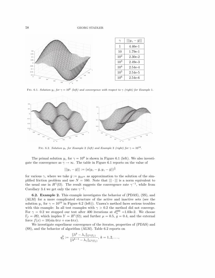
Fig. 6.1. Solution y! for ! = 108 (left) and convergence with respect to ! (right) for Example 1.

00.2

0.40.6

0.81

0

0.2

0.4

0.6

0.8

1-0. 3

-0. 2

-0. 1

0

0.1

0.2

00.2

0.40.6

0.81

0

0.2

0.4

0.6

0.8

1

-0. 2

-0. 1

0

0.1

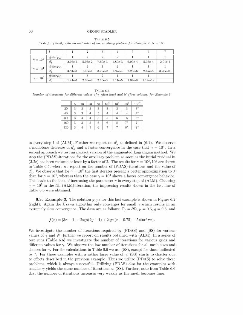
Fig. 6.2. Solution y! for Example 2 (left) and Example 3 (right) for ! = 1010.

The primal solution y" for % = 108 is shown in Figure 6.1 (left). We also investi-gate the convergence as % & '. The table in Figure 6.1 reports on the value of

|||y" ! y||| := (a(y" ! y, y" ! y))12

for various %, where we take y := y1016 as approximation to the solution of the sim-plified friction problem and use N = 160. Note that ||| · ||| is a norm equivalent tothe usual one in H1("). The result suggests the convergence rate %%1, while fromCorollary 3.4 we get only the rate %% 1

2 .

6.2. Example 2. This example investigates the behavior of (PDAS), (SS), and(ALM) for a more complicated structure of the active and inactive sets (see thesolution y" for % = 1010 in Figure 6.2 (left)). Uzawa’s method faces serious troubleswith this example: In all test examples with % > 0.2 the method did not converge.For % = 0.2 we stopped our test after 400 iterations at d400

! =1.03e-2. We choose#f = #", which implies Y = H1("); and further µ = 0.5, g = 0.4, and the externalforce f(x) = 10(sin 4-x + cos 4-x).

We investigate superlinear convergence of the iterates, properties of (PDAS) and(SS), and the behavior of algorithm (ALM). Table 6.2 reports on

qk! :=)"k ! "")L2("f )

)"k%1 ! "")L2("f ), k = 1, 2, . . . ,

SSN AND ALM FOR A SIMPLIFIED FRICTION PROBLEM 59

Table 6.2Values for qk" in Example 2, ! = 50.

k 1 2 3 4 5

qk" 0.58 0.45 0.25 0.18 0.00

Table 6.3Number of iterations of (SS) and (PDAS) for di!erent values of ! for Example 2, N = 160.

! 3 5 10 50 100 150 160 103 1010

#iterSS 3 4 4 5 6 7 div div div#iterPD 3 4 4 5 6 5 5 6 6

Table 6.4Tests for (ALM) with exact solve of the auxiliary problem for Example 2, N = 160.

l 1 2 3 4 5 6 7

#iterPD 6 3 2 1 1 1 1! = 102

dl" 2.55e-2 8.54e-3 3.62e-3 1.62e-3 7.45e-4 3.58e-4 1.77e-4

#iterPD 6 1 1 1 1! = 104

dl" 4.00e-4 3.06e-6 2.67e-8 2.62e-10 2.84e-12

for % = 50. We observe superlinear convergence of the iterates determined with (SS).Table 6.3 shows the number of iterations #iterSS and #iterPD required by (SS)

and (PDAS), respectively, to find the solution for di!erent values of %. We observea slight increase in the number of iterations as % increases. For % % 160 (SS) doesnot detect the solution, whereas (PDAS) does. Using (SS) for these examples wecan observe the following behavior: Points in #f move from Ak%1

% to Ak+, and then

from Ak+ back to Ak+1

% for some k % 2, and due to this scattering the algorithmdoes not find the solution (cf. the remark on the role of $ in (PDAS) after Lemma4.1). Algorithm (PDAS) with $ = 1 does not experience such problems and finds thesolution after a few iterations for all tested % > 0.

To avoid possible di$culties due to the local convergence of (SS), we test twoglobalization strategies: First we use a continuation procedure with respect to %,motivated from the local convergence result for (SS). We solve for % = 150 and usethe solution as initialization for the algorithm with larger %. This procedure turns outto be successful for only a moderate increase in %. Increasing % moderately, typicallyonly one or two more iterations are needed to find the solution for larger %. However,this method appears inconvenient and costly. Next we test backtracking with J" asmerit function to globalize (SS). This strategy works successfully, but in particularfor larger %, several backtracking steps are necessary in each iteration. The resultingstepsize is very small and thus overall up to 50 iterations are needed to find thesolution. This behavior becomes more distinct for large %.

We also apply algorithm (ALM) for the solution of this example. In a first attemptwe solve the auxiliary problem in (ALM) exactly using (PDAS), whereas this methodis initialized with the solution of the auxiliary problem in the previous iteration stepof (ALM). Due to the local superlinear convergence of (PDAS), the auxiliary problemis solved in very few iterations, as can be seen in Table 6.4, where for % = 102

and % = 104 we report on the number of iterations #iterPD required by (PDAS)

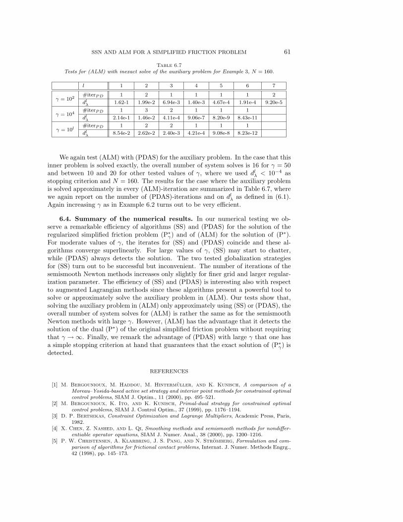
60 GEORG STADLER

Table 6.5Tests for (ALM) with inexact solve of the auxiliary problem for Example 2, N = 160.

l 1 2 3 4 5 6 7

#iterPD 1 2 2 2 1 1 1! = 102

dl" 2.96e-1 5.03e-2 7.60e-3 1.89e-3 9.99e-4 5.36e-4 2.91e-4

#iterPD 1 2 1 2 1 1 1! = 104

dl" 3.81e-1 1.46e-1 3.79e-2 1.87e-4 2.20e-6 2.67e-8 3.28e-10

#iterPD 1 3 2 1 1 1! = 10l

dl" 1.41e-1 2.30e-2 2.16e-3 1.11e-5 1.04e-8 1.14e-12

Table 6.6Number of iterations for di!erent values of ! (first line) and N (first column) for Example 3.

5 10 30 50 102 103 105 1010

20 3 3 3 3 3 3 3 3!

40 3 3 4 5 4 4 4 4!

80 3 4 4 5 5 6 6 6!

160 3 3 5 5 6 8 7! 7!

320 3 4 5 6 7 7 8! 8!

in every step l of (ALM). Further we report on dl! as defined in (6.1). We observea monotone decrease of dl! and a faster convergence in the case that % = 104. In asecond approach we test an inexact version of the augmented Lagrangian method: Westop the (PDAS)-iterations for the auxiliary problem as soon as the initial residual in(3.2c) has been reduced at least by a factor of 2. The results for % = 102, 104 are shownin Table 6.5, where we report on the number of (PDAS)-iterations and the value ofdl!. We observe that for % = 102 the first iterates present a better approximation to "than for % = 104, whereas then the case % = 104 shows a faster convergence behavior.This leads to the idea of increasing the parameter % in every step of (ALM). Choosing% = 10l in the lth (ALM)-iteration, the impressing results shown in the last line ofTable 6.5 were obtained.

6.3. Example 3. The solution y1010 for this last example is shown in Figure 6.2(right). Again the Uzawa algorithm only converges for small % which results in anextremely slow convergence. The data are as follows: #f = #", µ = 0.5, g = 0.3, and

f(x) = |3x! 1| + 2sgn(2y ! 1) + 2sgn(x! 0.75) + 5 sin(6-x).

We investigate the number of iterations required by (PDAS) and (SS) for variousvalues of % and N ; further we report on results obtained with (ALM). In a series oftest runs (Table 6.6) we investigate the number of iterations for various grids anddi!erent values for %. We observe the low number of iterations for all mesh-sizes andchoices for %. For the calculations in Table 6.6 we use (SS), except for those indicatedby !. For these examples with a rather large value of %, (SS) starts to chatter dueto e!ects described in the previous example. Thus we utilize (PDAS) to solve theseproblems, which is always successful. Utilizing (PDAS) also for the examples withsmaller % yields the same number of iterations as (SS). Further, note from Table 6.6that the number of iterations increases very weakly as the mesh becomes finer.

SSN AND ALM FOR A SIMPLIFIED FRICTION PROBLEM 61

Table 6.7Tests for (ALM) with inexact solve of the auxiliary problem for Example 3, N = 160.

l 1 2 3 4 5 6 7

#iterPD 1 2 1 1 1 1 2! = 102

dl" 1.62-1 1.99e-2 6.94e-3 1.40e-3 4.67e-4 1.91e-4 9.20e-5

#iterPD 1 3 2 1 1 1! = 104

dl" 2.14e-1 1.46e-2 4.11e-4 9.06e-7 8.20e-9 8.43e-11

#iterPD 1 2 2 1 1 1! = 10l

dl" 8.54e-2 2.62e-2 2.40e-3 4.21e-4 9.08e-8 8.23e-12

We again test (ALM) with (PDAS) for the auxiliary problem. In the case that thisinner problem is solved exactly, the overall number of system solves is 16 for % = 50and between 10 and 20 for other tested values of %, where we used dl! < 10%4 asstopping criterion and N = 160. The results for the case where the auxiliary problemis solved approximately in every (ALM)-iteration are summarized in Table 6.7, wherewe again report on the number of (PDAS)-iterations and on dl! as defined in (6.1).Again increasing % as in Example 6.2 turns out to be very e$cient.

6.4. Summary of the numerical results. In our numerical testing we ob-serve a remarkable e$ciency of algorithms (SS) and (PDAS) for the solution of theregularized simplified friction problem (P!

") and of (ALM) for the solution of (P!).For moderate values of %, the iterates for (SS) and (PDAS) coincide and these al-gorithms converge superlinearly. For large values of %, (SS) may start to chatter,while (PDAS) always detects the solution. The two tested globalization strategiesfor (SS) turn out to be successful but inconvenient. The number of iterations of thesemismooth Newton methods increases only slightly for finer grid and larger regular-ization parameter. The e$ciency of (SS) and (PDAS) is interesting also with respectto augmented Lagrangian methods since these algorithms present a powerful tool tosolve or approximately solve the auxiliary problem in (ALM). Our tests show that,solving the auxiliary problem in (ALM) only approximately using (SS) or (PDAS), theoverall number of system solves for (ALM) is rather the same as for the semismoothNewton methods with large %. However, (ALM) has the advantage that it detects thesolution of the dual (P!) of the original simplified friction problem without requiringthat % & '. Finally, we remark the advantage of (PDAS) with large % that one hasa simple stopping criterion at hand that guarantees that the exact solution of (P!

") isdetected.

REFERENCES

[1] M. Bergounioux, M. Haddou, M. Hintermuller, and K. Kunisch, A comparison of aMoreau–Yosida-based active set strategy and interior point methods for constrained optimalcontrol problems, SIAM J. Optim., 11 (2000), pp. 495–521.

[2] M. Bergounioux, K. Ito, and K. Kunisch, Primal-dual strategy for constrained optimalcontrol problems, SIAM J. Control Optim., 37 (1999), pp. 1176–1194.

[3] D. P. Bertsekas, Constraint Optimization and Lagrange Multipliers, Academic Press, Paris,1982.

[4] X. Chen, Z. Nashed, and L. Qi, Smoothing methods and semismooth methods for nondi!er-entiable operator equations, SIAM J. Numer. Anal., 38 (2000), pp. 1200–1216.

[5] P. W. Christensen, A. Klarbring, J. S. Pang, and N. Stromberg, Formulation and com-parison of algorithms for frictional contact problems, Internat. J. Numer. Methods Engrg.,42 (1998), pp. 145–173.

62 GEORG STADLER

[6] P. W. Christensen and J. S. Pang, Frictional contact algorithms based on semismooth New-ton methods, in Reformulation: Nonsmooth, Piecewise Smooth, Semismooth and Smooth-ing Methods, Appl. Optim. 22, M. Fukushima and L. Qi, eds., Kluwer Academic Publishers,Dordrecht, The Netherlands, 1999, pp. 81–116.

[7] P. W. Christensen, A nonsmooth Newton method for elastoplastic problems, Comput. Meth-ods Appl. Mech. Engrg., 191 (2002), pp. 1189–1219.

[8] G. Duvaut and J.-L. Lions, Inequalities in Mechanics and Physics, Springer-Verlag, Berlin,1976.

[9] I. Ekeland and R. Temam, Convex Analysis and Variational Problems, Classics Appl. Math.28, SIAM, Philadelphia, 1999.

[10] F. Facchinei and J.-S. Pang, Finite-Dimensional Variational Inequalities and Complemen-tarity Problems, Vol. 1 and 2, Springer Ser. Oper. Res., Springer-Verlag, New York, 2003.

[11] R. Glowinski, J.-L. Lions, and R. Tremolieres, Numerical Analysis of Variational Inequal-ities, North–Holland, Amsterdam, 1981.

[12] R. Glowinski, Numerical Methods for Nonlinear Variational Problems, Springer-Verlag, NewYork, 1984.

[13] W. Han, A regularization procedure for a simplified friction problem, Math. Comput. Mod-elling, 15 (1991), pp. 65–70.

[14] W. Han, On the numerical approximation of a frictional contact problem with normal compli-ance, Numer. Funct. Anal. Optim., 17 (1996), pp. 307–321.

[15] J. Haslinger, Z. Dostal, and R. Kucera, On a splitting type algorithm for the numericalrealization of contact problems with Coulomb friction, Comput. Methods Appl. Mech.Engrg., 191 (2002), pp. 2261–2281.

[16] M. Hintermuller, K. Ito, and K. Kunisch, The primal-dual active set strategy as a semis-mooth Newton method, SIAM J. Optim., 13 (2003), pp. 865–888.

[17] M. Hintermuller and G. Stadler, A semi-smooth Newton method for constrained linear-quadratic control problems, ZAMM Z. Angew. Math. Mech., 83 (2003), pp. 219–237.

[18] M. Hintermuller, A primal-dual active set algorithm for bilaterally control constrained opti-mal control problems, Quart. Appl. Math., 61 (2003), pp. 131–160.

[19] I. Hlavacek, J. Haslinger, J. Necas, and J. Lovisek, Solution of Variational Inequalitiesin Mechanics, Appl. Math. Sci. 66, Springer-Verlag, New York, 1988.

[20] H. C. Huang, W. Han, and J. S. Zhou, The regularization method for an obstacle problem,Numer. Math., 69 (1994), pp. 155–166.

[21] K. Ito and K. Kunisch, Augmented Lagrangian methods for nonsmooth, convex optimizationin Hilbert spaces, Nonlinear Anal., 41 (2000), pp. 591–616.

[22] K. Ito and K. Kunisch, Semi-smooth Newton methods for variational inequalities of the firstkind, M2AN Math. Model. Numer. Anal., 37 (2003), pp. 41–62.

[23] K. Ito and K. Kunisch, The primal-dual active set method for nonlinear optimal controlproblems with bilateral constraints, SIAM J. Control Optim., 43 (2004), pp. 357–376.

[24] N. Kikuchi and J. T. Oden, Contact Problems in Elasticity: A Study of Variational In-equalities and Finite Element Methods, SIAM Stud. Appl. Math. 8, SIAM, Philadelphia,1988.

[25] R. Kornhuber, Adaptive Monotone Multigrid Methods for Nonlinear Variational Problems,Adv. Numer. Math., Teubner, Stuttgart, 1997.

[26] R. Kornhuber, Monotone multigrid methods for elliptic variational inequalities. II, Numer.Math., 72 (1996), pp. 481–499.

[27] B. Kummer, Generalized Newton and NCP-methods: Convergence, regularity, actions, Discuss.Math. Di"er. Incl. Control Optim., 20 (2000), pp. 209–244.

[28] C.-Y. Lee and J. T. Oden, A priori error estimation of hp-finite element approximations offrictional contact problems with normal compliance, Internat. J. Engrg. Sci., 31 (1993),pp. 927–952.

[29] A. Y. T. Leung, G. Chen, and W. Chen, Smoothing Newton method for solving two- andthree-dimensional frictional contact problems, Internat. J. Numer. Methods Engrg., 41(1998), pp. 1001–1027.

[30] L. Qi and J. Sun, A nonsmooth version of Newton’s method, Math. Programming, 58 (1993),pp. 353–367.

[31] L. Qi, Convergence analysis of some algorithms for solving nonsmooth equations, Math. Oper.Res., 18 (1993), pp. 227–244.

[32] G. Savare, Regularity and perturbation results for mixed second order elliptic problems, Comm.Partial Di"erential Equations, 22 (1997), pp. 869–899.

[33] M. Ulbrich, Semismooth Newton methods for operator equations in function spaces, SIAM J.Optim., 13 (2003), pp. 805–841.