Embed Size (px)
Citation preview

The Kuratowski–Ryll-Nardzewski Theorem
and semismooth Newton methods for
Hamilton–Jacobi–Bellman equations
Iain Smears
INRIA Paris
Linz, November 2016
joint work with
Endre Suli, University of Oxford

Overview
Talk outline
1. Introduction: Howard’s algorithm / policy iteration for
Hamilton–Jacobi–Bellman equations.
2. Semismoothness of HJB operators in function spaces.
3. Applications to discontinuous Galerkin FEM approximations of HJB equations
with Cordes coefficients.
Overview
Talk outline
1. Introduction: Howard’s algorithm / policy iteration for
Hamilton–Jacobi–Bellman equations.
2. Semismoothness of HJB operators in function spaces.
3. Applications to discontinuous Galerkin FEM approximations of HJB equations
with Cordes coefficients.

1. Hamilton–Jacobi–Bellman Equation
F [u] := supα∈Λ
[Lαu − f α] = 0 in Ω,
u = 0 on ∂Ω,(HJB)
where Lαu := aα(x) : D2u + bα(x) · ∇u − cα(x) u.
Notation: aα(x) : D2u =d∑
i,j=1
aαij (x)uxi xj , bα(x) · ∇u =d∑
i=1
bαi (x)uxi .
Assumptions:
• bounded domain Ω,
• control set Λ is a compact metric space,
• continuous functions a, b, c and f in x ∈ Ω and α ∈ Λ.
Remark: Further assumptions are required for well-posedness of the problem, but
not for the semismoothness discussed here.
1/28

1. Motivation
Howard’s algorithm / policy iteration
Formal structure
1. Choose an initial guess u0.
2. For each k ≥ 0, choose αk : Ω→ Λ such that
αk(x) ∈ argmaxα∈Λ (Lαuk − f α)(x), ∀ x ∈ Ω.
3. Then, find uk+1 as a solution of the PDE
Lαkuk+1 = f αk in Ω, with uk+1 = 0 on ∂Ω,
where Lαk v := aαk (x)(x) : D2v + bαk (x)(x) · ∇v − cαk (x)v
In practice: used in a discrete context after discretization by a numerical method.
2/28
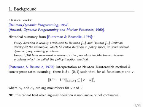
1. Background
Classical works:
[Bellman,Dynamic Programming, 1957]
[Howard, Dynamic Programming and Markov Processes, 1960].
Historical summary from [Puterman & Brumelle, 1979]:
Policy iteration is usually attributed to Bellman [...] and Howard [...] Bellman
developed the technique, which he called iteration in policy space, to solve several
dynamic programming problems.
Howard [16] later developed a version of this procedure for Markovian decision
problems which he called the policy-iteration method.
[Puterman & Brumelle, 1979]: interpretation as Newton–Kantorovich method &
convergence rates assuming: there is δ ∈ (0, 1] such that, for all functions u and v ,
‖Lαv − Lαu‖L(X ,Y ) . ‖v − u‖δX
where αv and αu are arg-maximisers for v and u.
NB: this cannot hold when arg-max operation is non-unique or not continuous.
3/28

1. Background
On solver algorithms for HJB: [Santos & Rust, 2004] Analysis of policy iteration
for finite dimensional MDP problems.
[Bokanowski, Maroso, Zidani, 2009]: Superlinear convergence and
semismoothness of finite dimensional HJB operators of form
minα∈AN
[Bαx− cα] = 0
with matrices Bα ∈ RN×N and vectors x, c ∈ RN , (see also discussion of
Bellman–Isaacs).
Variant algorithms and applications: penalty methods [Reisinger & Witte, 2011,
2012], coupled value-policy iteration [Alla, Falcone, Kalise, 2015]
Semismooth Newton methods [Ulbrich, 2002], [Hintermuller, Ito, Kunisch, 2002]
(primal-dual active set method as as semismooth Newton method)
4/28

1. Semismooth Newton methods
Notation: Let X and Y be sets. We write G : X ⇒ Y if G is a set-valued map
that maps X into the subsets of Y .
Definition of semismoothness [Ulbrich, 2002]
Let X and Y be Banach spaces.
Let F : X → Y .
Let DF : X ⇒ L(X ,Y ) with non-empty images.
We say that F is DF -semismooth on U if, for all x ∈ U,
lim‖e‖X→0
1
‖e‖Xsup L∈DF [u+e]‖F [u + e]− F [u]− L e‖Y = 0.
Then DF is then called a generalised differential of F on U.
Semismoothness + uniform stability of linearizations:
supL∈DF [v ],v∈X
‖L−1‖L(Y ,X ) <∞
=⇒ local superlinear convergence of semismooth Newton method.5/28
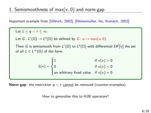
1. Semismoothness of max(v , 0) and norm-gap
Important example from [Ulbrich, 2002], [Hintermuller, Ito, Kunisch, 2002]
Let 1 ≤ q < r ≤ ∞.
Let G : Lr (Ω)→ Lq(Ω) be defined by G : u 7→ max(u, 0).
Then G is semismooth from Lr (Ω) to Lq(Ω) with differential DF [v ] the set
of all L ∈ L∞(Ω) of the form:
L(x) =
1 if v(x) > 0
0 if v(x) < 0
an arbitrary fixed value if v(x) = 0
Norm gap: the restriction q < r cannot be removed (counter-examples).
How to generalise this to HJB operators?
6/28

Overview
Talk outline
1. Introduction: Howard’s algorithm / policy iteration for
Hamilton–Jacobi–Bellman equations.
2. Semismoothness of HJB operators in function spaces.
3. Applications to discontinuous Galerkin FEM approximations of HJB equations
with Cordes coefficients.
7/28

1. Motivation
Howard’s algorithm / policy iteration
Formal structure
1. Choose an initial guess u0.
2. For each k ≥ 0, choose αk : Ω→ Λ such that
αk(x) ∈ argmaxα∈Λ (Lαuk − f α)(x), ∀ x ∈ Ω.
3. Then, find uk+1 as a solution of the PDE
Lαkuk+1 = f αk in Ω, with uk+1 = 0 on ∂Ω,
where Lαk v := aαk (x)(x) : D2v + bαk (x)(x) · ∇v − cαk (x)v
In practice: used in a discrete context after discretization by a numerical method.
8/28

2. Semismoothness of HJB operators
For FEM applications: let Th be a mesh on Ω.
Space X = W 2,r (Ω, Th), 1 ≤ r ≤ ∞, with norm:
‖u‖W 2,r (Ω;Th) =
∑K∈Th
‖u‖rW 2,r (K)
1r
.
Function u ∈W 2,r (Ω, Th) have element-wise gradient ∇hu and Hessian D2hu.
For Λ compact and continuous coefficients, F : W 2,r (Ω, Th)→ Lr (Ω) is well
defined and Lipschitz continuous
F [u] := supα∈Λ
[Lαu − f α].
9/28

2. Semismoothness: argmax set-valued map
For each u ∈ X , we define u =(u,∇hu,D
2hu)∈ Lr (Ω;Rm) for suitable m.
We then view the differential operator F [u] as a composition of x 7→ u(x) with the
scalar function F : Ω× Rm → R defined by
F (x , v) = supα∈Λ
[aα(x) : M + bα(x) · p − cα(x)z − f α(x)], v = (z , p,M)
Define the set-valued map Ω× Rm 3 (x , v) 7→ Λ(x , v) ⊂ Λ by
Λ(x , v) := argmaxα∈Λ[aα(x) : M + bα(x) · p − cα(x)z − f α(x)]
Straightforward: Λ(x , v) is non-empty and closed in Λ.
10/28

2. Semismoothness: argmax set-valued map
Important lemma:
The mapping Λ(·, ·) : Ω× Rm ⇒ Λ is upper semicontinuous:
For every (x , v) ∈ Ω×Rm, and any open neighbourhood U of Λ(x , v),
there is an open neighbourhood V of (x , v) such that Λ(y ,w) ⊂ U
for all (y ,w) ∈ V .
(x,v)
(xn,vn)
(xn,vn) ! (x,v)
10/28

2. Kuratowski–Ryll-Nardzewski Theorem
Kuratowski–Ryll-Nardzewski
Let Ω ⊂ Rd be a bounded open set,
let Λ be a compact metric space,
let Λ(·, ·) : Ω × Rm ⇒ Λ be an upper semicontinuous set-valued function,
such that Λ(x , v) is non-empty and closed for every (x , v) ∈ Ω× Rm.
Then, for any Lebesgue measurable function u : Ω → Rm, there exists a
Lebesgue measurable selection α : Ω→ Λ such that
α(x) ∈ Λ(x , u(x)
)for a.e. x ∈ Ω.
(Presented here in the form needed for our purposes - original result is rather more general)
Kuratowski & Ryll-Nardzewski, Bull. Acad. Polon. Sci., 1965:
A general theorem on selectors.
A (specialised) proof in Aubin & Cellina, Differential Inclusions, 1984.
11/28

2. The generalized differential of HJB operators
Recall u(x) = (u(x),∇hu(x),D2hu(x)) for u ∈W 2,r (Ω; Th).
Define the set of measurable selections Λ[u]:
Λ[u] = α : Ω→ Λ; α Lebesgue measurable, α(x) ∈ Λ(x , u(x)) a.e. in Ω .
Kuratowski–Ryll-Nardzewski Thm =⇒ Λ[u] is non-empty for all u ∈W 2,r (Ω; Th).
Define the differential
DF [u] := Lα = aα : D2h + bα · ∇h − cα, α ∈ Λ[u]
The measurability of α ∈ Λ[u] implies that Lα is well defined in
L(W 2,r (Ω; Th), Lr (Ω)).
12/28

2. Semismoothness of HJB operators
DF [u] := Lα = aα : D2h + bα · ∇h − cα, α ∈ Λ[u]
Theorem [S. & Suli, SINUM, 2014]
Let 1 ≤ q < r ≤ ∞.
The operator F : W 2,r (Ω; Th)→ Lq(Ω) is DF -semismooth on W 2,r (Ω; Th):
lim‖e‖
W 2,r (Ω;Th)→0
1
‖e‖W 2,r (Ω;Th)
supLα∈DF [u+e]
‖F [u + e]− F [u]− Lαe‖Lq(Ω) = 0.
Remark: The sup implies any choice of measurable selection is sufficient.
I. S. & E. Suli, SIAM J. Numer. Anal. 2014:
Discontinuous Galerkin finite element approximation of Hamilton–Jacobi–Bellman
equations with Cordes coefficients.
13/28
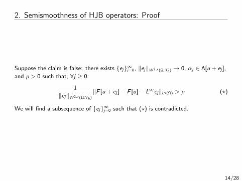
2. Semismoothness of HJB operators: Proof
Suppose the claim is false: there exists ej∞j=0, ‖ej‖W 2,r (Ω;Th) → 0, αj ∈ Λ[u + ej ],
and ρ > 0 such that, ∀j ≥ 0:
1
‖ej‖W 2,r (Ω;Th)
‖F [u + ej ]− F [u]− Lαj ej‖Lq(Ω) > ρ (?)
We will find a subsequence of ej∞j=0 such that (?) is contradicted.
14/28

2. Semismoothness of HJB operators: Proof
1. Passing to a subsequence, we have (ej ,∇hej ,D2hej)→ 0 pointwise a.e. in Ω.
2. Key inequality: using the definition of F , we can show (pointwise):
|F [u+ej ](x)−F [u](x)−Lαj ej(x)| ≤ |Lαej(x)−Lαj ej(x)| ∀α ∈ Λ(x , u(x)), a.e. x .
This implies
|F [u + ej ]− F [u]− Lαj ej | . Gj (|ej |+ |∇ej |+ |D2hej |), (??)
where the function Gj is defined by:
Gj := infα∈Λ(·,u(·))
|aα − aαj |+ |bα − bαj |+ |cα − cαj | .
Remark: Gj is measurable (can be written as a composition of a lower
semicontinous function with measurable functions).
15/28

2. Semismoothness of HJB operators: Proof
Recall Gj := infα∈Λ(·,u(·)) |aα − aαj |+ |bα − bαj |+ |cα − cαj |.Recall also αj(x) ∈ Λ(x , u(x) + ej(x)) for a.e. x ∈ Ω.
(x,u)
(x,u(x) + ej(x))
(x,u(x) + ej(x)) ! (x,u(x))
Upper semi-continuity of Λ(·, ·) leads to
Gj → 0 pointwise a.e. in Ω.
16/28

2. Semismoothness of HJB operators: Proof
Also, we have a uniform bound supj≥0‖Gj‖L∞(Ω) ≤ C because all coefficients are
uniformly bounded on Ω× Λ.
Lebesgue’s Dominated Convergence Theorem:
limj→∞‖Gj‖Ls (Ω) = 0 for any 1 ≤ s <∞.
Recall (??):
|F [u + ej ]− F [u]− Lαj ej | . Gj (|ej |+ |∇ej |+ |D2hej |), (??)
If q < r , Holder’s inequality implies that we can find s ∈ [1,∞) s.t.
0 < ρ ≤ 1
‖ej‖W 2,r (Ω;Th)
‖F [u + ej ]− F [u]− Lαj ej‖Lq(Ω) ≤ ‖Gj‖Ls (Ω) → 0.
Remarks: the norm gap appears because there are cases where ‖Gj‖L∞(Ω) 6→ 0.
17/28

2. Semismoothness of HJB operators
DF [u] := Lα = aα : D2h + bα · ∇h − cα, α ∈ Λ[u]
Theorem [S. & Suli, SINUM, 2014]
Let 1 ≤ q < r ≤ ∞.
The operator F : W 2,r (Ω; Th)→ Lq(Ω) is DF -semismooth on W 2,r (Ω; Th):
lim‖e‖
W 2,r (Ω;Th)→0
1
‖e‖W 2,r (Ω;Th)
supLα∈DF [u+e]
‖F [u + e]− F [u]− Lαe‖Lq(Ω) = 0.
Remark: The sup implies any choice of measurable selection is sufficient.
I. S. & E. Suli, SIAM J. Numer. Anal. 2014:
Discontinuous Galerkin finite element approximation of Hamilton–Jacobi–Bellman
equations with Cordes coefficients.
18/28

Overview
Talk outline
1. Introduction: Howard’s algorithm / policy iteration for
Hamilton–Jacobi–Bellman equations.
2. Semismoothness of HJB operators in function spaces.
3. Applications to discontinuous Galerkin FEM approximations of HJB equations
with Cordes coefficients.
19/28

3. Cordes condition
From now on, we suppose
• Ω is bounded Lipschitz domain
• aα uniformly elliptic, cα ≥ 0, uniformly over Ω×.
Policy iteration:
Lαkuk+1 = f αk , αk ∈ Λ[uk ]
Is this linear PDE well-posed for general uniformly elliptic coefficients aα?
In general: no! Due to discontinuities in aα:
• Non-uniqueness of strong solutions [Gilbarg & Trudinger, 2001]
• Non-uniquess of viscosity solutions [Nadirashvili, 1997], [Safonov, 1999].
However: yes under a further assumption:
• Cordes condition (next slide) : well-posedness in H2(Ω) ∩ H10 (Ω).
20/28

3. Cordes condition
From now on, we assume that Ω is convex:
Cordes condition: Case 1: without advection and reaction
Assume that there exists ε ∈ (0, 1] s. t.
|aα(x)|2(Tr aα(x))2 ≤
1
d − 1 + ε∀ x ∈ Ω, α ∈ Λ. (Cordes0)
Cordes condition: Case 2: extension to bα 6= 0 and cα 6= 0
Assume that there exist λ > 0 and ε ∈ (0, 1] s. t.
|aα|2 + |bα|2/2λ+ (cα/λ)2
(Tr aα + cα/λ)2≤ 1
d + εin Ω, ∀α ∈ Λ. (Cordes1)
Thm: [Cordes 1956], [Maugeri, Palagachev, Softova 2000]
There is C = C(ε) s.t. for any measurable α→ Λ:
‖(Lα)−1‖L2→H2∩H10≤ C .
21/28

3. Cordes condition
Well-posedness theorem [S. & Suli, SINUM, 2014]
Under these assumptions, there exists a unique u ∈ H2(Ω) ∩ H10 (Ω) that
solves (HJB) pointwise a.e. in Ω.
Remarks
• If dimension d = 2, (Cordes0) ⇐⇒ uniform ellipticity.
• Proof is based on Cordes condition and Miranda–Talenti inequality for convex
domains:
|u|H2(Ω) := ‖D2u‖L2(Ω) ≤ ‖∆u‖L2(Ω) ∀ u ∈ H2(Ω) ∩ H10 (Ω).
22/28

3. Applications to numerical scheme
Construction an hp-version discontinuous Galerkin finite element scheme in [S. &
Suli, SINUM 2013 + SINUM 2014 + Num. Math. 2016]:
• Discrete Stability in H2: uh is uniquely defined, and stable in discrete
norm ‖·‖H2(Ω;Th) + |·|Jh .
• Consistency for true solution : if u ∈ Hs(Ω, Th) with s > 5/2.
• Near-best approximation w.r.t H2-conforming subspaces.
• Convergence rates: if u ∈ Hs(Ω, Th) with s > 5/2:
‖u − uh‖H2(Ω;Th) .hmin(p+1,s)−2
ps−5/2‖u‖Hs (Ω).
Main idea: based on approximating a strongly monotone operator formulation of
the PDE:
A(u; v) =
∫Ω
supα∈Λ
[γα(Lαu − f α)](∆v − λv)dx = 0 ∀v ∈ H2(Ω) ∩ H10 (Ω);
23/28

3. Applications to numerical scheme
Discrete linearised problems:
Akh(uk+1
h , vh) =∑K∈Th
〈γαk f αk , Lλvh〉K ∀ vh ∈ Vh,p,
where the bilinear form Akh : Vh,p × Vh,p → R is defined by
Akh(wh, vh) :=
∑K∈Th
〈(γαkLαkwh, Lλvh〉K + linear stabilization terms from Ah(·; ·).
Superlinear convergence [S. & Suli, SINUM, 2014]
There exists R > 0, possibly depending on h and p, such that
if ‖uh − u0h‖H2(Ω;Th) < R, then superlinear convergence:
limk→∞
‖uh − uk+1h ‖H2(Ω;Th)
‖uh − ukh‖H2(Ω;Th)
= 0
24/28
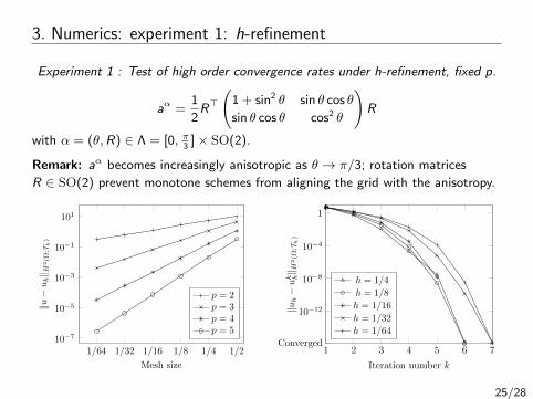
3. Numerics: experiment 1: h-refinement
Experiment 1 : Test of high order convergence rates under h-refinement, fixed p.
aα =1
2R>(
1 + sin2 θ sin θ cos θ
sin θ cos θ cos2 θ
)R
with α = (θ,R) ∈ Λ = [0, π3
]× SO(2).
Remark: aα becomes increasingly anisotropic as θ → π/3; rotation matrices
R ∈ SO(2) prevent monotone schemes from aligning the grid with the anisotropy.
1/21/41/81/161/321/6410−7
10−5
10−3
10−1
101
Mesh size
‖u−
uh‖ H
2(Ω
;Th
)
p = 2p = 3p = 4p = 5
1 2 3 4 5 6 7Converged
10−12
10−8
10−4
1
Iteration number k
‖uh−uk h‖ H
2(Ω
;Th
)
h = 1/4
h = 1/8
h = 1/16
h = 1/32
h = 1/64
25/28

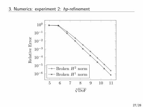
3. Numerics: experiment 2: hp-refinement
Experiment 2: test of exponential convergence rates under hp-refinement
Let Ω = (0, 1)2, bα := (0, 1), cα := 10 and define
aα := α>(
20 1
1 0.1
)α, α ∈ Λ := SO(2), λ =
1
2.
(Cordes1) holds with ε ≈ 0.0024 (nearly degenerate, strongly anisotropic).
Solution:
u(x , y) = (2x − 1)(e1−|2x−1| − 1
)(y +
1− ey/δ
e1/δ − 1
), δ := 0.005 = O(ε)
• Near-degenerate and anisotropic diffusion.
• Sharp boundary layer.
• Non-smooth solution.
26/28

3. Numerics: experiment 2: hp-refinement
Experiment 2: test of exponential convergence rates under hp-refinement
Let Ω = (0, 1)2, bα := (0, 1), cα := 10 and define
aα := α>(
20 1
1 0.1
)α, α ∈ Λ := SO(2), λ =
1
2.
(Cordes1) holds with ε ≈ 0.0024 (nearly degenerate, strongly anisotropic).
Solution:
u(x , y) = (2x − 1)(e1−|2x−1| − 1
)(y +
1− ey/δ
e1/δ − 1
), δ := 0.005 = O(ε)
Boundary layer adapted meshes with p-refinement: 2 ≤ pK ≤ 10, from 100 to
1320 DoFs.
26/28
3. Numerics: experiment 2: hp-refinement
5 6 7 8 9 10 11
10−6
10−5
10−4
10−3
10−2
10−1
100
3√DoF
RelativeError
Broken H2 norm
Broken H1 norm
27/28
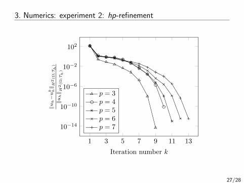
3. Numerics: experiment 2: hp-refinement
1 3 5 7 9 11 13
10−14
10−10
10−6
10−2
102
Iteration number k
‖uh−uk h‖ H
2(Ω
;Th
)
‖uh‖ H
2(Ω
;Th
)
p = 3p = 4p = 5p = 6p = 7
27/28

Conclusions
Conclusions:
• General semismoothness result for HJB operators with Λ a general compact
metric space and continuous coefficients.
• Usage of the measurable selection theorem of Kuratowski–Ryll-Nardzewski.
• Application to DGFEM for HJB equations with Cordes coefficients: superlinear
convergence of the semismooth Newton method
• Numerical experiments showing fast convergence and weak dependence of the
iteration counts on h and p.
Linear nondivergence form PDE: Discontinuous Galerkin finite element
approximation of nondivergence form elliptic equations with Cordes coefficients, I. S.
& E. Suli, SIAM J. Numer. Anal. 2013.
Elliptic HJB: Discontinuous Galerkin finite element approximation of
Hamilton–Jacobi–Bellman equations with Cordes coefficients, I. S. & E. Suli, SIAM
J. Numer. Anal. 2014.
Parabolic HJB: Discontinuous Galerkin finite element methods for time-dependent
Hamilton–Jacobi–Bellman equations with Cordes coefficients, I. S. & E. Suli,
Numerische Mathematik 2016.
Thank you!28/28

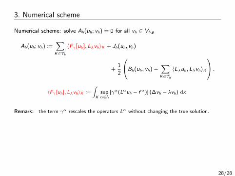
3. Numerical scheme
Numerical scheme: solve Ah(uh; vh) = 0 for all vh ∈ Vh,p
Ah(uh; vh) :=∑K∈Th
〈Fγ [uh], Lλvh〉K + Jh(uh, vh)
+1
2
Bh(uh, vh)−∑K∈Th
〈Lλuh, Lλvh〉K
.
28/28
3. Numerical scheme
Numerical scheme: solve Ah(uh; vh) = 0 for all vh ∈ Vh,p
Ah(uh; vh) :=∑K∈Th
〈Fγ [uh], Lλvh〉K + Jh(uh, vh)
+1
2
Bh(uh, vh)−∑K∈Th
〈Lλuh, Lλvh〉K
.
〈Fγ [uh], Lλvh〉K :=
∫K
supα∈Λ
[γα(Lαuh − f α)] (∆vh − λvh) dx .
Remark: the term γα rescales the operators Lα without changing the true solution.
28/28

3. Numerical scheme
Numerical scheme: solve Ah(uh; vh) = 0 for all vh ∈ Vh,p
Ah(uh; vh) :=∑K∈Th
〈Fγ [uh], Lλvh〉K + Jh(uh, vh)
+1
2
Bh(uh, vh)−∑K∈Th
〈Lλuh, Lλvh〉K
.
Jump penalisation with µF ' p2K/hK and ηF ' p4
K/h3K for F ⊂ ∂K :
Jh(uh, vh) :=∑
F∈F i,bh
[µF 〈J∇T uhK, J∇T vhK〉F + ηF 〈JuhK, JvhK〉F
]+∑F∈F i
h
µF 〈J∇uh · nF K, J∇vh · nF K〉F .
28/28

3. Numerical scheme
Numerical scheme: solve Ah(uh; vh) = 0 for all vh ∈ Vh,p
Ah(uh; vh) :=∑K∈Th
〈Fγ [uh], Lλvh〉K + Jh(uh, vh)
+1
2
Bh(uh, vh)−∑K∈Th
〈Lλuh, Lλvh〉K
.
〈Lλuh, Lλvh〉K :=
∫K
(∆uh − λuh) (∆vh − λvh) dx .
28/28

3. Numerical scheme
Numerical scheme: solve Ah(uh; vh) = 0 for all vh ∈ Vh,p
Ah(uh; vh) :=∑K∈Th
〈Fγ [uh], Lλvh〉K + Jh(uh, vh)
+1
2
Bh(uh, vh)−∑K∈Th
〈Lλuh, Lλvh〉K
.
Weak enforcement of Miranda–Talenti inequality:
Bh(uh, vh) :=∑K∈Th
[〈D2uh,D
2vh〉K + 2λ〈∇uh,∇vh〉K + λ2〈uh, vh〉K]
+∑F∈F i
h
[〈divT∇Tuh, J∇vh · nF K〉F + 〈divT∇Tvh, J∇uh · nF K〉F
]−
∑F∈F i,b
h
[〈∇T∇uh · nF , J∇T vhK〉F + 〈∇T∇vh · nF , J∇T uhK〉F
]− λ
∑F∈F i,b
h
[〈∇uh · nF , JvhK〉F + 〈∇vh · nF , JuhK〉F ]
− λ∑F∈F i
h
[〈uh, J∇vh · nF K〉F + 〈vh, J∇uh · nF K〉F ]
28/28

3. Numerical scheme
Numerical scheme: solve Ah(uh; vh) = 0 for all vh ∈ Vh,p
Ah(uh; vh) :=∑K∈Th
〈Fγ [uh], Lλvh〉K + Jh(uh, vh)
+1
2
Bh(uh, vh)−∑K∈Th
〈Lλuh, Lλvh〉K
.
Consistency, Stability, Convergence rates [S. & Suli, SINUM, 2014]
• Discrete Stability: uh is uniquely defined, and stable in discrete norm
‖·‖H2(Ω;Th) + |·|Jh .
• Consistency: Ah(u; vh) = 0 for the solution u, if u ∈ Hs(Ω, Th) with
s > 5/2.
• Near-best approximation w.r.t H2-conforming subspaces.
• Convergence rates: ‖u − uh‖H2(Ω;Th) .hs
ps−1/2 ‖u‖Hs (Ω) if
u ∈ Hs(Ω, Th) with s > 5/2.
28/28

3. Discrete Semismooth Newton method
Algorithm
1. Choose an initial guess u0h ∈ Vh,p.
2. Given ukh ∈ Vh,p, k ∈ N, choose αk ∈ Λ[uk
h ].
3. Solve
Akh(uk+1
h , vh) =∑K∈Th
〈γαk f αk , Lλvh〉K ∀ vh ∈ Vh,p,
where the bilinear form Akh : Vh,p × Vh,p → R is defined by
Akh(wh, vh) :=
∑K∈Th
〈(γαkLαkwh, Lλvh〉K + linear stabilization terms from Ah(·; ·).
Well-posedness : the bilinear forms Akh(·, ·) have a uniform coercivity constant.
Superlinear convergence [S. & Suli, SINUM, 2014]
There exists R > 0, possibly depending on h and p, such that
if ‖uh − u0h‖H2(Ω;Th) < R, then uk
h → uh superlinearly.
28/28