Scholars' Mine Scholars' Mine

Masters Theses Student Theses and Dissertations

Fall 2016

Sensitivity analysis of geomechanical parameters in a two-way Sensitivity analysis of geomechanical parameters in a two-way

coupling reservoir simulation coupling reservoir simulation

Hector Gabriel Donoso

Follow this and additional works at: https://scholarsmine.mst.edu/masters_theses

Part of the Petroleum Engineering Commons

Department: Department:

Recommended Citation Recommended Citation Donoso, Hector Gabriel, "Sensitivity analysis of geomechanical parameters in a two-way coupling reservoir simulation" (2016). Masters Theses. 7596. https://scholarsmine.mst.edu/masters_theses/7596

This thesis is brought to you by Scholars' Mine, a service of the Missouri S&T Library and Learning Resources. This work is protected by U. S. Copyright Law. Unauthorized use including reproduction for redistribution requires the permission of the copyright holder. For more information, please contact scholarsmine@mst.edu.

SENSITIVITY ANALYSIS OF GEOMECHANICAL PARAMETERS IN A TWO-

WAY COUPLING RESERVOIR SIMULATION

by

HECTOR GABRIEL DONOSO GOMEZ

A THESIS

Presented to the Faculty of the Graduate School of the

MISSOURI UNIVERSITY OF SCIENCE AND TECHNOLOGY

In Partial Fulfillment of the Requirements for the Degree

MASTER OF SCIENCE IN PETROLEUM ENGINEERING

2016

Approved by

Dr. Peyman Heidari, Advisor

Dr. Ralph Flori

Dr. Baojun Bai

ii

2016

Hector Gabriel Donoso Gomez

All Rights Reserved

iii

ABSTRACT

Currently reservoir simulators model geomechanical effects such as compaction,

subsidence, fault reactivation, breach of the seal integrity, etc. using only the rock

compressibility to change the pore volume. However, rock compressibility as a scalar

quantity is unfit to represent the true rock mechanics in the reservoir. In order to

accurately represent geomechanical effects in a reservoir simulation, a two-way coupling

simulation of the stress analyzer and the reservoir simulator was done. Based on the

poroelasticity theory during the production or depletion of the reservoir the porosity and

permeability changed due to the stress or pore pressure changes.

A sensitivity analysis was carried out in order to understand how geomechanical

parameters impact reservoir performance under a certain set of assumptions. In the

material modeling steps elastic and plastic rocks were created for the simulation. The

Mohr-Coulomb failure criterion was implemented for the yield criteria of the materials.

Sensitivity analysis study enabled us to understand why stress changes, rock

deformation and rock failure occur during the depletion of the reservoir. Engineers will

also be able to prevent disasters because different ranges of rock mechanics were

identified as key factors in vertical displacement and stress changes in the reservoir.

Overall, geomechanical parameters directly affecting reservoir performance will be

identified and therefore improved due to this study.

iv

ACKNOWLEDGEMENTS

I would first like to thank my thesis advisor Dr. Peyman Heidari, for his guidance

and assistance. He allowed me to research my own topic and develop my own work, but

he always directed me to the right direction when I was struggling.

My research wouldn’t have been completed without the help of my committee

members Dr. Baojun Bai and Dr. Ralph Flori. They always showed a sense of

encouragement and support toward my work.

I would also like to acknowledge my colleagues: Kelsi Leverett, Sameer

Salasakar, Mahta Ansari, Pu Han, Yao Wang and Hasan Al-Saedi.

Lastly I want to acknowledge my wife, parent and brother for their endless

support.

v

TABLE OF CONTENTS

Page

ABSTRACT ……………………………………………………………………………iii

ACKNOWLEDGEMENTS ………………………………………………………………iv

LIST OF FIGURES ……...……………………………………………………………...vii

LIST OF TABLES ……………………………………………………………………….ix

NOMENCLATURE ……………………………………………………………………...xi

SECTION

1. INTRODUCTION …………………………………………………………………...1

1.1 MOTIVATION .....................................................................................................4

1.2 OUTLINE OF THE THESIS ................................................................................5

2. RESERVOIR GEOMECHANICS …………...……………………………………...6

2.1 TERZAGHI’S PRINCIPLE ..................................................................................6

2.2 RESERVOIR COMPACTION AND SUBSIDENCE .........................................7

2.3 STRESS ................................................................................................................8

2.3.1 Principal Stress..........................................................................................9

2.3.2 In-situ Stress..............................................................................................9

2.3.3 E. M. Anderson Classification ................................................................10

2.4 MOHR CIRCLE .................................................................................................10

2.5 FAULT REGIME ...............................................................................................10

2.6 STRAIN ..............................................................................................................12

2.7 CONSTITUTIVE LAWS ...................................................................................14

2.8 ELASTIC DEFORMATION ..............................................................................14

2.9 PLASTIC DEFORMATION ..............................................................................15

2.10 POROELASTIC DEFORMATION ...................................................................15

2.11 VISCOELASTIC DEFORMATION ..................................................................16

3. CREATING A GEOMECHANICAL GRID……………………………………. 18

3.1 RESERVOIR GRID............................................................................................18

3.2 MAKE/EDIT GEOMECHANICAL GRID ........................................................18

vi

3.2.1 Sideburden ..............................................................................................20

3.2.2 Overburden .............................................................................................22

3.2.3 Underburden ...........................................................................................24

3.3 MATERIAL MODELING..................................................................................26

3.3.1 Material Library ......................................................................................26

3.3.2 Defining Loading Conditions .................................................................29

3.3.3 Pressure, Temperature and Water Saturation ..........................................31

3.3.4 Boundary Conditions ..............................................................................31

3.3.5 Simulation Case ......................................................................................32

3.3.6 Running The Simulation .........................................................................33

4. COUPLING IN A POROUS MEDIA ……………………………………………35

4.1 HYDRO-MECHANICAL COUPLING .............................................................35

4.2 PERMEABILITY UPDATING METHOD ........................................................36

4.3 POROSITY UPDATING METHOD .................................................................37

5. RESULTS AND DISCUSSION ………………………………………………….39

5.1 CASE 1: RESERVOIR VS TWO WAY COUPLING SIMULATION .............39

5.2 CASE 2: SENSITIVITY ANALYSIS OF GEOMECHANICAL

PARAMETERS ..................................................................................................41

5.2.1 Case 2A: Young Modulus Alteration .....................................................44

5.2.2 Case 2B: Poisson’s Ratio Alteration .......................................................47

5.2.3 Case 2C: Biot’s Coefficient Alteration ...................................................49

5.3 CASE 3: FACIES SENSITIVITY ANALYSIS .................................................49

5.4 CASE 4: CORRELATION ANALYSIS OF GEOMECHANICAL

PARAMETERS ..................................................................................................50

6. CONCLUSION AND RECOMMENDATIONS ………………………………...61

BIBLIOGRAPHY ………………………………………………………………………..63

VITA ……………………………………………………………………………………..65

vii

LIST OF FIGURES

Page

Figure 1.1: Displacement fields for a uniform pressure drawdown.....................................2

Figure 2.1: Terzaghi's principle ...........................................................................................7

Figure 2.2: In-situ stress (O'Connell 1994) ........................................................................10

Figure 2.3: E. M. Andersonian classification scheme taken from (Anderson 1951) .........11

Figure 2.4: Reverse faulting regime found in Gullfaks reservoir ......................................11

Figure 2.5: Stresses acting on a solid (Ingebritsen and Sanford 1998) ..............................12

Figure 2.6: Stress vs Strain curve for Steel ........................................................................16

Figure 2.7: Viscoelastic Stress vs Strain Curve .................................................................17

Figure 3.1: Gullfak's Reservoir Grid ..................................................................................19

Figure 3.2: Geomechanical Grid of Model ........................................................................20

Figure 3.3: Stress deforming side burden ..........................................................................21

Figure 3.4: Example of rotational angle of grid .................................................................22

Figure 3.5: Overburden surfaces ........................................................................................23

Figure 3.6: Finalized overburden grid ...............................................................................24

Figure 3.7: Underburden surfaces ......................................................................................25

Figure 3.8: Finalized underburden grid .............................................................................25

Figure 3.9: Top view of reservoir (Duncan, Wright et al.) and top view of reservoirs

faults (left) ........................................................................................................30

Figure 5.1: Well A16 cumulative oil production (sm3) of regular reservoir simulation

(blue) and of coupled simulation with geomechanics included (red). .............40

Figure 5.2: Well A16 cumulative gas production (sm3) of regular reservoir simulation

(blue) and of coupled simulation with geomechanics included (red). .............41

Figure 5.3: Well A12 cumulative oil production (sm3) of regular reservoir simulation

(blue) and of coupled simulation with geomechanics included (red). .............43

Figure 5.4: Well A12 cumulative gas production (sm3) of regular reservoir simulation

(blue) and of coupled simulation with geomechanics included (red). .............43

Figure 5.5: Well A12 Cumulative oil production Young Modulus change. ......................46

Figure 5.6: Well A12 Cumulative gas production Young Modulus change......................46

Figure 5.7: Well A12 Cumulative oil production Poisson’s ratio change. ........................51

viii

Figure 5.8: Well A12 Cumulative gas production Poisson’s ratio change.. ......................51

Figure 5.9: Well A12 Cumulative oil production Biot’s Coefficient change. ...................53

Figure 5.10: Well A12 Cumulative gas production Biot’s Coefficient change. ................54

Figure 5.11: Facies distribution present in reservoir model. .............................................55

Figure 5.12: Average permeability rate of change for sand facies ....................................56

Figure 5.13: Average permeability rate of change for fine silt facies ...............................57

Figure 5.14: Average permeability rate of change for clay facies .....................................57

Figure 5.15: Average permeability rate of change for silt facies .......................................58

ix

LIST OF TABLES

Page

Table 3.1: Sideburden elasticity model properties .............................................................27

Table 3.2: Overburden elasticity model properties ............................................................27

Table 3.3: Underburden elasticity model properties ..........................................................28

Table 3.4: Plates elasticity model properties .....................................................................29

Table 3.5: Reservoir grid elasticity model property ranges ...............................................29

Table 3.6: Fault discontinuity parameters ..........................................................................30

Table 3.7: Pressure data in bar’s for each time-step ..........................................................34

Table 5.1: Cumulative oil production for both simulations ...............................................42

Table 5.2: Cumulative gas production for both simulations ..............................................42

Table 5.3: Min and max value for geomechanical parameters altered ..............................44

Table 5.4: Cumulative oil and gas production for Case 2A and control simulation

(Case Ct) ..........................................................................................................45

Table 5.5: Cumulative oil production by individual well for changes in Young

Modulus ...........................................................................................................47

Table 5.6: Cumulative gas production by individual well for changes in young

modulus ............................................................................................................48

Table 5.7: Cumulative oil and gas production for all Case 2B and control simulation

(Case Ct) ..........................................................................................................50

Table 5.8: Cumulative oil production by individual well for changes in Poisson’s ratio ..52

Table 5.9: Cumulative gas production by individual well for changes in Poisson’s

ratio ..................................................................................................................53

Table 5.10: Cumulative oil and gas production for all Case 2C and control simulation

Case Ct) ............................................................................................................54

Table 5.11: Cumulative oil production by individual well for changes in Biot’s

coefficient. .......................................................................................................55

Table 5.12: Cumulative gas production by individual well for changes in Biot’s

coefficient ........................................................................................................56

Table 5.13: Cumulative oil and gas production for simulations with variations in its

Young Modulus ...............................................................................................58

x

Table 5.14: Cumulative oil and gas production for simulations with variations in its

Poisson’s ratio ..................................................................................................59

Table 5.15: Cumulative oil and gas production for simulations with variations in its

Biot’s coefficient ..............................................................................................59

Table 5.16: Correlation analysis of elastic geomechancial parameters .............................60

xi

NOMENCLATURE

Symbol Description

ф Porosity

cr Compressibility factor

p Pressure (bar)

p0 Initial Pressure (bar)

Vp Pore Volume

Vb Bulk Volume

Vb0 Initial Bulk Volume

σ Stress

SH Maximum horizontal stress

Sh Minimum stress

Sv Vertical stress

ρ Density

z Depth (meters)

g Gravity (m/s2)

ρw Density of water

zw Water depth

ϵ Strain

A Stress path

Pp Pore pressure

α Biot’s Coefficient

F Force

k Spring Constant

X Distance

Kt Bulk Modulus of dry rock

Ks Bulk Modulus of mineral

xii

PVf Final Pore Volume

PV0 Initial Pore Volume

PVcor Pore Volume corrected

1

1. INTRODUCTION

Geomechanics made its initial appearance in the oil and gas industry when

engineers where planning how to perform a successful hydraulic fracturing. Hydraulic

fracturing will occur when the pressure of the injected fluid creates enough force so that

it exceeds the tensile strength of the rock surrounding the wellbore. Once this occurs the

rock will fail and create fractures which will travel through the area of the rock with the

least resistance. So stimulation engineers had to fully understand the formations stresses

in order to have an estimate of the pressure needed to fracture the rock and in which

directions the fractures would tend to occur.

From here several new areas in the oil and gas industry started to use the

understanding of rock mechanics to their benefit. But the main focus of Geomechanics

was simply to understand the rock surrounding the wellbore. The stress field of the

overall reservoir was never looked as being of importance. Until disasters started to occur

due to reservoir production and depletion. The geomechanical effects that are caused by

reservoir production are fault reactivation, breach of the seal integrity, well failure,

bedding parallel slip, subsidence and compaction. Compaction itself will possibly lead to

subsidence of the overburden, also a reduction in permeability and porosity. The most

famous disaster due to subsidence was in the Ekofisk oil fields (Sulak and

Petroleum,1991) which happened in the North Sea. Subsidence can lead to possible

damage to your well and equipment. This is because the reservoir will be moving

downwards but the drilling or completion equipment remains stationary and could be

crushed by the added weight. Fault reactivation can definitely affect wellbore stability,

fluid leakage into the surface and cause subsidence. These are all problems that can be

dealt with accordingly if the simulation model can accurately estimate when, why and

where they are going to occur.

Currently reservoir simulations try to simulate these geomechanical effects using

only the rock compressibility in order to change the pore volume. Rock compressibility is

the only rock mechanics parameter in the entire reservoir simulation. Being only a scalar

quantity it is unfit to represent the true rock mechanics in the reservoir. Several

2

assumptions are made when using this methodology. The total stress is assumed to be

constant and also the loading conditions inside the reservoir are supposed to be the same

as in the laboratory where simple loading is applied to a core sample in order to calculate

the rock compressibility. The basic approach is to create the problem into a 1D problem

meaning that there only a vertical deformation of the rock and also that each column of

grid-blocks will deform independently of each other. In Figure 1.1 an axisymmetric disc

shaped reservoir is placed under a pressure drawdown that is happening uniformly

throughout the model. The model shows that the overburden will not deform the same

way in every grid block column (Gutierrex & Lewis,1998).

Figure 1.1: Displacement fields for a uniform pressure drawdown

In a reservoir a uniaxial test can be done to acquire geomechanical properties

from the rocks. The uniaxial tests consists of simply applying a load in the vertical

direction to a core sample in order to monitor the deformation of the rock and when rock

failure occurs. The test results that this experiment can yield are uniaxial compressive

strength, Young modulus and Poisson ratio. So technically the rock surrounding the core

sample is not taken into consideration making the rock compressibility which was

calculated in the lab a rough estimate of the real rock compressibility.

3

In a standard reservoir simulation the rock compressibility changes the porosity as

seen in the following equation:

Φ = Φ0[1 + 𝑐𝑟 (𝑝 − 𝑝0) (1)

This shows that porosity is a function of pressure which depends also on the rock

compressibility of the rock. The equation for calculating the pore volume of the grid-

blocks is the following:

𝑉𝑝 = 𝑉𝑏0Φ (2)

The previous equation is incorrect because the pore volume actually deforms due

to various stresses applied to the rock, pore pressure variations and temperature changes

to some extent. This deformation happens due to Terzaghi’s principle of effective stress

(Terzaghi, 1966). The actual equation should look like the following (Toshiaki, Saito and

Sumihiko,2003):

𝑉𝑏 = 𝑉𝑏0(1 − 𝜀𝑣) (3)

The true porosity is later calculated as:

Φ = 𝑉𝑝/𝑉𝑏 (4)

Now pore volume and the porosity are a function of stress as well. This new

relationship is written as the following:

Φ =𝑉𝑝

𝑉𝑏= 𝑓(𝑝, 𝑇, 𝜎); 𝑉𝑝 = 𝑓(𝑝, 𝑇, 𝜎) (5)

Since most reservoir models don’t allow for a change in pore volume during the

simulation run a pseudo porosity is created to recalculate the volumes correctly (Settari

and Walters,2001) using the following equation:

Φ∗ =𝑉𝑝

𝑉𝑏 (6)

The real issue is running a reservoir simulation that can update its rock

compressibility and porosity after each time-step; after a stress analysis program has

calculated the displacement field, stress and strain parameters. For this to occur you need

a platform software that has two engine software’s that can run the reservoir simulation

and the stress analysis at the same time. Both of them have to interchange information in

order to change the porosity and permeability of the reservoir simulation. But the porosity

should be changing due to the new stresses and rock compressibility calculated by the

4

stress analyzer. The sharing and updating of parameters between both engines is called

two-way coupling.

This paper focuses on using a newly developed coupling software created by

Schlumberger called Reservoir Geomechanics. It is an optional module in the Petrel E&P

platform. The module was created as a response of Schlumberger acquiring the Visage

Finite element software (engine) on 2007 which would help solve stress equations and

help relate how reservoir parameters can be a function of stress variation. Petrel E&P

having ECLIPSE (engine) as its reservoir simulator needed a stress analyzer and a

coupling program that could link these software’s all together. Therefore the Reservoir

Geomechanics module was created for two main reasons. The module will take a 3D

model created in Petrel E&P and alter it in order for it to run with Visage. Then it also

has to act as the coupling program between Eclipse and Visage.

By doing a two way coupling simulation it is possible to predict stress changes,

rock deformation and rock failure that might occur in the future due to depletion.

Engineers will also be able to take into account compaction and subsidence in the

reservoir simulation. This is important because it determines the well completions

survivability, vertical displacement movement and reservoir performance. It also gives

the opportunity of performing a sensitivity analysis in order to determine how parameters

alter reservoir performance.

1.1 MOTIVATION

Currently less than 5% of all reservoir simulations have been coupled with a

stress analyzer in order to correctly model the deformation of rocks and there effects on

the permeability of the reservoir. It is believed that two way coupling simulations are a

waste of time and money in most reservoir simulations. This is the case because most of

the research on the benefits and consequences of running a coupled simulations are done

only in homogeneous or perfectly layered models which do not model actual reservoirs

accurately. This is why this research focuses on using the Gullfaks reservoir.

By using an existing reservoir model people will see how much a typical reservoir

model might overestimate its cumulative oil and gas production.

5

1.2 OUTLINE OF THE THESIS

The structure of the thesis is as follows:

• Section 1 presents a general discussion, beginning with the overall concept of

how geomechanics has its place in the in the oil and gas industry. Next, the

motivation for this work and an outline of the thesis is presented.

• Section 2 discusses basic reservoir geomechanics principles which help

understand why a stress analyzer is used in order to properly model the

permeability reduction of a reservoir during its depletion. Terzaghis principle is

explained and the possible benefits/consequences of reservoir compaction.

• Section 3 explains step by step how to transform a reservoir model into a

geomechanical model. This includes the creation of the side, under and over

burden. All of the geomechanical parameters included into the model and the

boundary condition used for the simulation. An explanation of how the

permeability and porosity is also included in this section.

• Section 4 describes how the coupling occurs in a porous media. The equations

used in a hydro-mechanical coupling are displayed and explained. Also the

function used for the permeability updating and how it works is explained.

• Section 5 displays and explains the results of the research. The section explains all

of the different cases created in order to display how coupled simulations can alter

the reservoir performance drastically.

• Section 6 is the last section which focuses on providing conclusions from the

results. Any recommendations based on the research and follow ups will be

explained as well.

6

2. RESERVOIR GEOMECHANICS

During the production or depletion of a reservoir several geomechanical effects

may occur but the main ones focused in this research are compaction and subsidence of

the subsurface. If subsidence occurs in the ground level it is directly related to a

compaction occurring in the reservoir due to the production of gas, hydrocarbons or

water. These geomechanical effects are rarely seen as a problem in the industry because

the level of compaction of a reservoir is usually insignificant, so the probability of any

serious subsidence occurring is rare. But ground subsidence cannot be overlooked

because reports have shown that entire surfaces have been vertically displaced about 10

meters. Recent examples of subsidence can be seen in the North Sea on the Valhall and

Ekofisk reservoirs. In order for subsidence to occur in this magnitude several conditions

have to be present.

In a way subsidence can be prevented if proper water flooding is implemented in

the reservoir in order to prevent a drastic pressure drop. Preventing pore pressure drops

are important because it is a key factor in the deformation of the rock (Terzaghi, 1925).

This deformation of the rock will have a direct impact in reservoir performance. This

occurs because the permeability and tortuosity of the reservoir is affected.

During the depletion of a reservoir there are temperature, pressure and saturation

changes. These changes have an effect on the stress state of the reservoir and its

surroundings (Zoback 2007). This section focuses on explaining what stress is and how it

behaves in the subsurface. The E. M. Anderson’s classification scheme is also explained

in order to understand how principal stresses act during a normal, strike-slip or reverse

faulting.

2.1 TERZAGHI’S PRINCIPLE

Karl Von Terzaghi stated that when a rock is subjected to a force in the

subsurface it is opposed by the pressure of the fluid inside the pores of the rock. The

equation in order to determine the effective stress can be seen in Figure 2.1. The total

7

stress applied to a rock is subtracted by the pore pressures force in order to determine the

effective stress. For Terzaghi “effective” stress is used to determine changes in volume,

shape or strength of the rock.

Figure 2.1: Terzaghi's principle

The pore pressure acts as a force that maintains the rocks in place and preventing

them from deforming. As the pore pressure differential increases the effective stress will

also increase meaning that there is more room for deformation. When a rock deforms by

expansion it can close pore throats due to the reduction in porosity. This means that the

porosity and permeability will be altered.

2.2 RESERVOIR COMPACTION AND SUBSIDENCE

Reservoir compaction is a volumetric change of the reservoir due to the

production or depletion of a reservoir. Subsidence is the lowering or change of level of

the surface which is a result of the compaction of the subsurface. In reservoirs

compaction and subsidence can cause serious economic consequences due to a reduction

in permeability. But they are not always negative consequences. As compaction of the

reservoir occurs the porosity of the rock reduces. This reduction in porosity may lead to

8

an increase in pressure which actually acts as a production drive mechanism. (Doornhof,

Kristiansen et al. 2006).

Compaction drive occurs when the expulsion of the reservoir fluid within a rocks

pore is caused by the reduction in pore volume. This will only have a significant increase

in production if the pore compressibility is high. This usually occurs in shallow or

unconsolidated reservoirs where the rock is able to compress further than a deep

consolidated reservoir. In some cases compaction can lead to 50 to 80% of the reservoirs

total energy (Settari 2013).

2.3 STRESS

It is possible to imagine stress as being the force that deforms a material (Davis

and Reynolds 1996). The deformation of the material will occur if the strength is

surpassed. The actual definition is the force that acts on a given area. Stress is commonly

represented by the σ symbol and the equation that defines it is the following:

σ =𝐹𝑜𝑟𝑐𝑒

𝐶𝑟𝑜𝑠𝑠−𝑆𝑒𝑐𝑡𝑖𝑜𝑛𝑎𝑙 𝐴𝑟𝑒𝑎 (7)

In this paper stress will be represented in the SI unit mega Pascal’s represented as

MPa. The English unit for stress is psi, where 145 psi = 1MPa respectively. Stresses can

be seen as a tensor which represents all of the forces passing through a single point

(Zoback 2007). The stress will be used to calculate the deformation of the rock which is

represented as strain. This is why ts necessary to use Visage as the geomechancail

simulator so that it can calculate the volumetric strain which represents the change in

porosity. Without it the updating of the permeability through the two-way coupling

simulation would not be possible. It would have to be estimated by the rock

compressibility or a permeability updating table which could be included in the reservoir

simulation without the addition of geomechanics. But these tables are based on mostly

homogeneous and isotropic materials and are never as accurate as running a two-way

coupling simulation in order to properly model the deformation of the rock. In order to

properly model permeability loss stress paths have to be modeled as well.

9

2.3.1 Principal Stress. In order to accurately describe the state of stress of a

point in the subsurface three stress tensors where created. They are the maximum,

intermediate and minimum principal stresses. In order to label a stress as a principal

stress they have to be occurring in a free surface which means that the tangential forces

are negligible at this plane (O'Connell 1994, Doornhof, Kristiansen et al. 2006). This

occurs below the surface so this is one of the reasons E. M. Anderson’s used principal

stresses in order to classify relative stress magnitudes in normal, strike-slip and reverse

faults. Principal stresses are also used in the field of reservoir geomechanics and will be

used in this research

2.3.2 In-situ Stress. There are several ways of viewing stress as a measurement

but for this research in-situ stresses will be used to describe the stresses at the sub

surface. This is because in-situ stresses can be represented by only three orthogonal

principal stresses where no shear stress occurs (Jaeger, Cook et al. 2007). The three

principal stresses are labeled as Sv, SH and Sh. These are the vertical, maximum horizontal

and minimum horizontal stress respectively. Assuming the surface is flat and that no

shear stresses develop Sv is seen as the overburden stress that is applied to the reservoir.

Then the minimum and maximum horizontal stresses are orthogonal to the vertical stress

as can be seen in Figure 2.2. Also stresses applied to a cube can be seen in Figure 2.5.

In order to calculate Sv the integral of the rock densities ρ taken from the surface

to the desired depth z.

𝑆𝑣 = ∫ 𝜌(𝑧)𝑔𝑑𝑧𝑧

0 (8)

In this equation g is the gravitational acceleration and the density is the function

of the depth. But if the calculation has to be made for a reservoir in the offshore there is a

water correction that has to be implemented into the equation.

𝑆𝑣 = 𝜌𝑤𝑔𝑧𝑤 + ∫ 𝜌(𝑧)𝑔𝑑𝑧𝑧

0 (9)

In this new equation ρw is the density of water and it is multiplied by g and zw

which is the water depth. The first part of the equation adds the force of the overlying

water that is on top of the surface and the density of water is estimated to be 1 g/cm3.

Usually the pressure of a column of water increases by 0.44 psi/ft.

10

Figure 2.2: In-situ stress (O'Connell 1994)

2.3.3 E. M. Anderson Classification. E. M. Anderson came up with a

classification in order to understand how stress magnitudes should form due to three

faulting regimes. These three are normal, strike-slip and reverse faulting. In a normal

fault regime σ1 is the vertical stress and σ3 is the minimum horizontal stress. A strike-slip

fault regime has σ1 as maximum horizontal stress and σ3 as the minimum horizontal

stress. The last fault regime is reverse faulting here σ1 is maximum horizontal stress and

σ3 is the vertical stress. A clear image of the regimes can be seen in Figure 2.3.

2.4 MOHR CIRCLE

During changes of stresses on a geological formation faulting may occur. This

happens during reservoir depletion which alters the pressure in the sub surface. This can

cause faulting which can alter reservoir performance. In order to understand and visualize

when faulting would occur a tool was created Otto Mohr (Mohr 1882).

2.5 FAULT REGIME

The fault regime for the Gullfaks reservoir is of reverse faulting which indicates

that the principal stress with the highest force is SH. The principal stress with the least

11

force will be SV, a better picture of the faulting regime can be viewed in Figure 2.4. The

boundary conditions used for the simulation can be seen in Section 3.3.4.

Figure 2.3: E. M. Andersonian classification scheme taken from (Anderson 1951)

Figure 2.4: Reverse faulting regime found in Gullfaks reservoir

12

2.6 STRAIN

Stress changes can alter or deform a solid. This deformation is expressed as the

strain a solid has gone through. For example if a vertical load is applied to a solid it will

start to deform in its height by shrinking. If the stress being applied to a solid are as the

following:

The strain is calculated by taking the distance the solid shrunk labeled w and

dividing it by the original height of the solid before the loading occurred. This can also be

calculated using the same method for each direction:

𝜀𝑥𝑥 = 𝛛𝐮

𝛛𝐱 𝜀𝑦𝑦 =

𝛛𝐯

𝛛𝐲 𝜀𝑧𝑧 =

𝛛𝐰

𝛛𝐳 (10)

In this equation u, v and w represent the displacement after a stress change. Then

the final strain for each direction is represented by ϵxx, ϵyy and ϵzz. In order to get the total

volumetric strain ϵv one has to add all of the strains in each direction”

𝜀𝑥𝑥 + 𝜀𝑦𝑦 + 𝜀𝑧𝑧 = 𝜀𝑣 (11)

Figure 2.5: Stresses acting on a solid (Ingebritsen and Sanford 1998)

13

In order to calculate shear strain which do not occur in right angles a new set of

equations can be used.

𝜀𝑥𝑦 = 1

2

𝛛𝐮

𝛛𝐲+

𝛛𝐯

𝛛𝐱, 𝜀𝑥𝑧 =

1

2

𝛛𝐯

𝛛𝐳 +

𝛛𝐰

𝛛𝐱, 𝜀𝑦𝑧 =

1

2

𝛛𝐯

𝛛𝐳+

𝛛𝐰

𝛛𝐲 (12)

This implies that shear strain is half the increase in a starting right angle

measurement with respect to the coordinate system.

Changes may occur in the reservoir stress paths by depletion. In order to

understand how stress paths change during depletion the poroelastic theory is used. This

means that the reservoir would be isotropic, linearly elastic and it would extend infinitely

horizontally. Also it is assumed that when the reservoir pressure reduces by a value of

“x”, the effective vertical stress increases by this same value of “x”. This is basically

stated by Terzaghi’s principle (Terzaghi 1966). For simplicity Biot’s coefficient is

assumed to be unity. There is also no strain in the horizontal planes. If we take into

consideration all of the previous assumptions to be true it is possible to state the

following.

∆𝜎′𝐻 − 𝑣∆𝜎′ℎ − 𝑣∆𝜎′𝑉 = 0 (13)

And

∆𝜎′ℎ − 𝑣∆𝜎′𝐻 − 𝑣∆𝜎′𝑉 = 0 (14)

Since there is no strain in this model v poisons ratio would become 0 and

therefore it is possible to say that changes in the minimum and maximum horizontal

effective stress are the same.

∆𝜎′𝐻 = ∆𝜎′ℎ (15)

The relationship between the effective horizontal stresses and the effective

vertical stress is given by:

∆𝜎′𝐻 = ∆𝜎′ℎ = (𝑣

1−𝑣) ∗ ∆𝜎′𝑉 (16)

The equation can be simplified so that the stress path A can be calculated with

any of the horizontal stresses and the pore pressure Pp.

14

𝐴 =∆𝑆𝐻𝑜𝑟

∆𝑃𝑝= (

1−2𝑣

1−𝑣) (17)

𝐴 =∆𝑆𝐻𝑜𝑟

∆𝑃𝑝= 𝛼 (

1−2𝑣

1−𝑣) (18)

If Biot’s coefficient is not unity the formula can be changed into the following. It

is important to remember that the vertical stress is constant during depletion when the

horizontal extent of the reservoir is infinite. If this is not the case the vertical stress will

not maintain constant during depletion. But it has been proven that if the ratio between

lateral extent and the width is greater than 10:1 the vertical stress will act as a constant

stress as well. The overall stress path results will be almost identical to a reservoir with

an infinite lateral extension. These stress path equation should not be used in a real life

situation because no reservoir is isotropic, inelastic, and homogeneous or is laterally

extended infinitely.

2.7 CONSTITUTIVE LAWS

A constitutive law states how a rock deforms when a stress is applied to it. Since

all rocks are not the same they deform in various ways. It is important to know how a

rock will deform because during depletion the reservoir will undergo compaction and

subsidence. Compaction can lead to an enhancement in production. But it can also affect

the permeability of the rocks drastically. If subsidence occurs there might be wellbore

stability issues or induced faulting. The most basic way for a rock to deform in a

reservoir is elastically.

2.8 ELASTIC DEFORMATION

When a force is applied to a material it will start to deform. If the force being

applied to the material is released and the material returns to its original state it means it

deformed elastically. If this occurs and the stress vs strain is linearly proportional the

deformation is categorized as being a linearly elastic material. The linear elastic

deformation is governed by Hooke’s Law.

𝐹 = 𝑘𝑋 (19)

15

In Hooke’s Law the force is labeled as F, k is the spring constant and X is the

displacement of the spring. In order to translate this equation to a rock mechanics point of

view the equation is written as:

𝜎 = 𝐸ϵ (20)

Here the stress σ becomes the force being applied to the material. The constant of

proportionality which is represented by k in Hooke’s law is changed to E representing the

materials Young modulus. Since strain ϵ also measured deformation it replaces X in

Hooke’s law.

2.9 PLASTIC DEFORMATION

During an elastic deformation the material will return to its original state. But if

the material does not return to its original state after the force is released it means it

underwent plastic deformation which is irreversible. When stress is increasing there will

be a yield point where the slope of the line (young modulus) begins to change. The

change occurs because the material has gotten to a point where it will deform at a higher

pace as the stress increases. Any deformation occurring after the yield point is labeled as

plastic deformation. During the plastic deformation two things can occur. The material

can start to undergo strain hardening which is when atomic dislocation can increase the

strength of the material allowing it to deform less as stress is increased. If after the yield

point the material deforms rapidly the material has started to undergo necking which is

caused because a reduction in the cross sectional area of the material. It doesn’t matter if

necking or strain hardening occurs during the process the final stage is when the material

fractures at the end. The stress versus strain graph for steel can be seen in Figure 2.6.

2.10 POROELASTIC DEFORMATION

Rocks especially in reservoirs will have pores saturated with fluids. This fluid will

allow the rock to deform in a poroelastic behavior meaning that the rate of speed the

force is applied to the material will cause a different results. Meaning that the stiffness of

the material is related to how the force is being applied. If the force is applied slowly to

16

the material the fluid inside the pore is allowed to drain out (drained) of the material so it

does not influence the overall stiffness of the rock.

Figure 2.6: Stress vs Strain curve for Steel

The rock would deform as if no liquids where present in the pores. But when

force is applied to a material rapidly and the liquid is not allowed to drain (undrained) the

pore pressure increases. The result would be an increase of the overall strength of the

rock and a reduction in the deformation rate. In order for this deformation too take place

the material should have interconnected pores which are saturated with a fluid. Also the

volume of the pore spaces is smaller than the total volume of the rock.

2.11 VISCOELASTIC DEFORMATION

This deformation is similar to the elastic deformation but instead it’s when a

viscous material has irreversible deformation after a force is applied to it. How the rock

responds is also related to the rate of speed of the load being applied to the material and

also the viscosity. When a load is applied quickly the rocks behaves stiffer than when a

load is applied slowly. Then the viscosity acts as a second stiffness factor that comes into

17

effect after the material has surpassed its yield point. A highly viscous material will

respond by deforming at higher stresses than a less viscous material. This response can be

viewed in the stress vs strain curve in Figure 2.7.

Figure 2.7: Viscoelastic Stress vs Strain Curve

18

3. CREATING A GEOMECHANICAL GRID

Reservoir simulations have different governing equations and numerical methods

than geomechanical modeling. This means that the reservoir grid has to undergo some

modifications before any geomechanical analysis is possible. The addition of an over,

under and side burden to the reservoir grid is necessary. There will be a significant

increase in computations done by the computer due to the increasing in size of the grid

and the number of grid blocks. Calculations are more complicated and more factors have

to be taken into consideration. This is one of the main reasons companies decide not to do

geomechanical analysis of their reservoir, it takes at least ten times more than a standard

simulation. The initial reservoir grid was built using Petrel and the actual simulation was

completed using Eclipse. Inside Petrel a new module (Reservoir Geomechanics) was used

in order to create the geomechanical grid. This is the first step in order to run a

geomechanical analysis.

3.1 RESERVOIR GRID

The reservoir grid is based on the geological model of the reservoir. The

geological model usually consists of horizons which are representing bedding planes and

also contain faults. The reservoir grid will attempt to recreate as accurately as possible

the geological formations. No model is an exact replica of a real world reservoir but the

closer you get to it the more accurate your findings will be during the simulation. The

purpose of the grid is so that the fluid flow equations of the geological model can be

solved.

3.2 MAKE/EDIT GEOMECHANICAL GRID

Once the reservoir simulation is finished the new geomechanical grid feature is

available in Petrel. It is in charge of adding a under, over and side burden to the previous

reservoir grid. The thickness of the model has to be relatively thick so that any substantial

buckling can be avoided. The change in grid is also done so that the far field stresses

19

caused by the boundary conditions are not felt by the reservoir directly. It is unrealistic to

place the stress and loading conditions directly into each of the reservoirs grid blocks.

Stress would never be dispersed equally along each of the grid blocks so it is necessary to

expand the grid in order to make the simulation as close to real life as possible. The

recommended aspect ratio (horizontal to vertical) is of 3 to 1. By doing this the model

will be excessively deep which is done on purpose. This extra underburden is labeled as

the bedrock which acts as a stiff rock that helps prevent buckling. The stiff rock below

will resist deforming therefore preventing buckling form occurring. The reservoir grid

representing the Gullfak’s reservoir used for this research can be seen in Figure 3.1.

Figure 3.1: Gullfak's Reservoir Grid

This is the reservoir grid without any of the geomechanical modifications done to

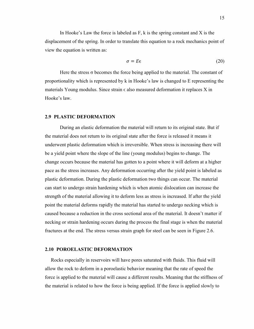
it. The finalized geomechanical grid can be seen in Figure 3.2. The workflow in order to

create this finalized grid is explained in detail throughout Section 3.

20

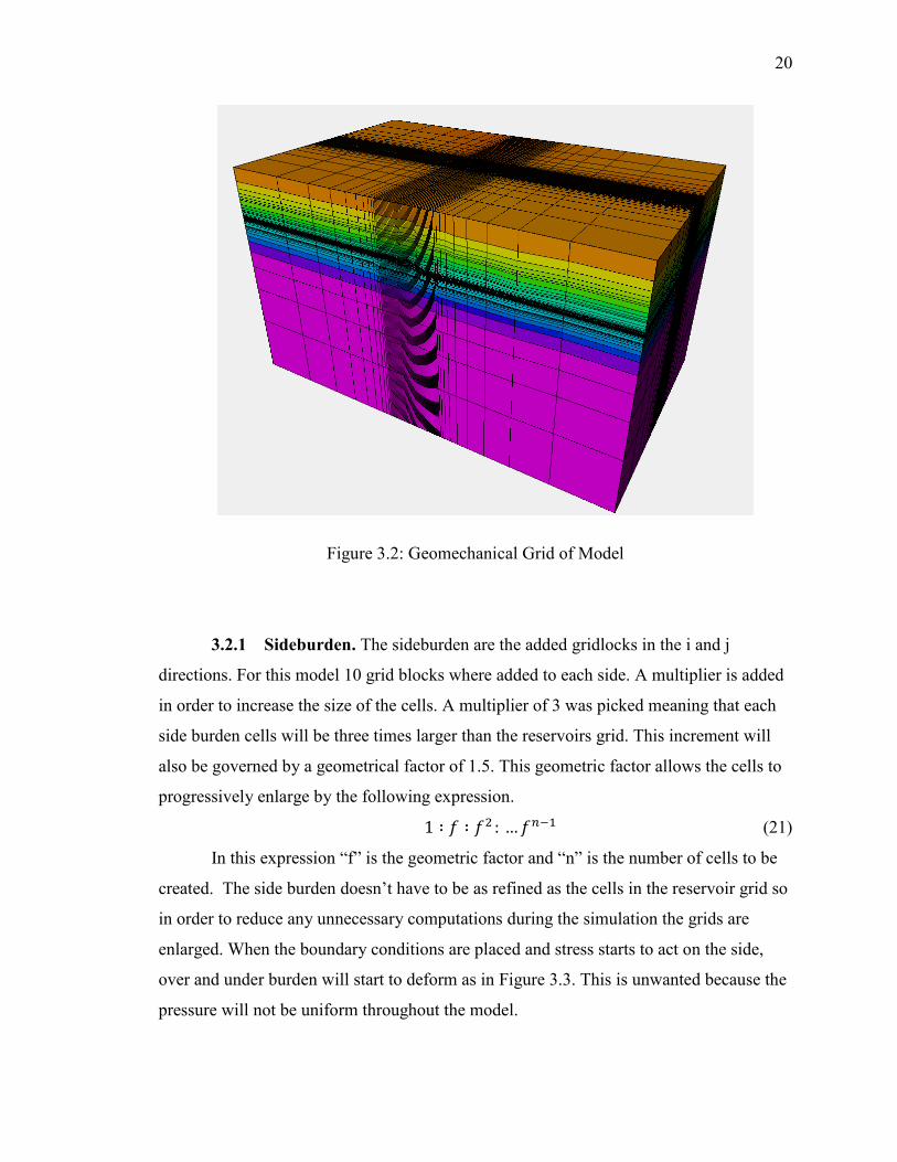
Figure 3.2: Geomechanical Grid of Model

3.2.1 Sideburden. The sideburden are the added gridlocks in the i and j

directions. For this model 10 grid blocks where added to each side. A multiplier is added

in order to increase the size of the cells. A multiplier of 3 was picked meaning that each

side burden cells will be three times larger than the reservoirs grid. This increment will

also be governed by a geometrical factor of 1.5. This geometric factor allows the cells to

progressively enlarge by the following expression.

1 ∶ 𝑓 ∶ 𝑓2 : … 𝑓𝑛−1 (21)

In this expression “f” is the geometric factor and “n” is the number of cells to be

created. The side burden doesn’t have to be as refined as the cells in the reservoir grid so

in order to reduce any unnecessary computations during the simulation the grids are

enlarged. When the boundary conditions are placed and stress starts to act on the side,

over and under burden will start to deform as in Figure 3.3. This is unwanted because the

pressure will not be uniform throughout the model.

21

Figure 3.3: Stress deforming side burden

As seen in Figure 3.3 once the stress is applied to the model the top region

deforms because of the pressure gradient that was placed in the boundary condition. The

rock in the bottom is denser and can withstand more stress before deforming. So in order

to prevent this deformation two stiff plates are added to the sides of the model. These stiff

plates are incompetent rocks that will not deform during compression so the stress can be

more uniformly distributed to the model. These stiff plates have to have a young modulus

of 1.5 times larger than the highest young modulus in the model. The plate thickness

picked for this model was of 50 meters and with a Young modulus of 52.5.

When the reservoir grid was created a rotation of -30 degrees was implemented

into it. This was probably done in order for the reservoir to fit into a geological formation

or other neighboring grids. In order to quickly figure out the rotation there is a feature

called “calculate angle from grid” in the first menu. It is possible to view how the side

burden is added to a grid with a rotation. In Figure 3.4 the reservoir grid can be seen with

a rotation (a). When the rotation is calculated the software can build a sideburden with

the same rotation so that it meshes accurately with the reservoir grid (b).

22

Figure 3.4: Example of rotational angle of grid

3.2.2 Overburden. The overburden is the overlaying rock of the reservoir. It

should be from the top of the reservoir to the surface. Adding an overburden allows for

the correct calculation of the vertical stress using equation 6. The overburden was done

differently from the side burden. For the overburden you have the option of creating it

based on surfaces and then in between each surface there is the option of adding grid

blocks. Three surfaces that emulate the reservoir shape are used for this step. The first

surface was created at a depth between 267 and 695 meters (orange). The second surface

is at a depth of 1,003 and 1,503 meters (yellow). The third surface created was at a depth

of 1,500 and 2,030 meters (light green). These surfaces all are a perfect copy of the

reservoir surface. This is why each surface has a depth range. It is possible to view each

of the surfaces with respect to the reservoir which is located at the bottom in Figure 3.5.

23

Figure 3.5: Overburden surfaces

Then the number of cells can be placed each division of surfaces. There are four

areas in which cells need to be distributed. The first area is from the surface level of 0

meters to the first overburden surface. For this depth range 1 division was made with a

geometric factor of 1.5. There is no need for a fine grid when close to the boundary

conditions because the fine grid should only be done when close to the reservoir. Any

additional cells will only increase the simulation time. Going from the first overburden to

the second overburden surface 5 divisions were created with a geometric factor of 1.5.

This would be the second area in the overburden. The third area is in-between the second

and third overburden surface. In this area 5 divisions were made and each one was

distributed by a geometric factor of 1.5. The last area would be in between the third

overburden surface till the actual reservoir. Here 6 divisions were made and distributed

by a geometric factor of 1.5. This increment will also be governed by a geometrical

factor of 1.5. The final overburden of the model can be seen in Figure 3.6. It is possible to

view how the grid becomes finer as it nears the acual reservoir in order to properly model

the stress paths found in he reservoir. Also to reduce simulation time because no real

calculations have to be done to grid blocks near the perimeter of the model.

24

Figure 3.6: Finalized overburden grid

3.2.3 Underburden. For the underburden two surfaces were created in order for

the cell distribution. The first surface is at a depth of 2,050 and 2,700 meters (light blue).

The following surface was created in between the depths 2,750 and 3,350 meters (dark

blue). These surfaces can be seen in respect to the reservoir grid in Figure 3.7.

The cells for the underburden start from the reservoir to the first underburden

surface with the light blue color. For his area 10 divisions were created with a

geometrical factor of 1.5. The next area is in between the two surfaces created for the

underburden. Here 8 divisions were created with a geometrical factor of 1.5. The last area

is from the deepest surface to a depth of 9,500 meters. In here 5 divisions were created

with a geometrical factor of 1.5. It is possible to view the finalized underburden in Figure

3.8. It is similar to the overburden but is extended in the z direction further due to not

having a height constraint. The overburden can only extend to the top of the reservoir

while the underburden has a wider range of freedom for the z direction. This flexibility

allows you to build the model three times larger than the reservoir grid. Therefore

satisfying the general rule of thumb that states that the geomechanical model has to be at

least three times larger than the reservoir model.

25

Figure 3.7: Underburden surfaces

Figure 3.8: Finalized underburden grid

26

3.3 MATERIAL MODELING

Once the geomechanics grid is created material modeling is needed in order to

create the materials that will be introduced into each cell. In the previous steps the cells

were created but the type of rocks and its geomechanical parameters have not yet been

assigned. Materials are created in order to place them into the overburden, sideburden,

underburden and the plates. These materials will specify if they are elastic or plastic

material. If a material is elastic the young modulus, Poisson’s ratio, bulk density and the

Biot’s elastic coefficient is needed. If the material deforms plastically the elastic

parameters are still needed but a yield criteria is also required. Depending on which

failure criteria is picked different yield criteria properties will be needed. In this research

only the Mohr-Coulomb failure criterion is used. With this failure model it is necessary to

place the unconfined compressive stress, friction angle, dilation angel, tensile stress

cutoff and hardening/softening coefficient.

3.3.1 Material Library. Petrel already has some predetermined materials which

are saved into the material library. Since most of the rocks surrounding the reservoir

might be unknown it is safe to place the predetermined materials in Petrel for the side,

under, or overburden. But if the specific geomechanical parameters surrounding the

reservoir are known it is possible to create a new material and introduce them into the

model. There are also a list of typical rocks found in the subsurface. For example there

are predetermined materials for sandstone, siltstone, shale, salt, limestone, chalk and clay.

These materials can be deform plastically and elastic. Also the faults have predetermined

materials as well.

For this research the predetermined materials found in the material library were

used for the side, over and underburden. The geomechanical parameters for each material

can be seen in Table 3.1, Table 3.2, and Table 3.4. It is important to remember that all of

these materials where heterogeneous but once they were changed they became

homogeneous. These changes will alter te reservoir performance, this change will be

measured in order to see which parameter alters reservoir performance the most out of all

the paramters. The parameters altered are Young modulus, Poisson’s ratio and Biot’s

coefficient.

27

Table 3.1: Sideburden elasticity model properties

Property Value Unit

Young Modulus 25 GPa

Poisson’s Ratio 0.25

Bulk Density 2.304 g/cm3

Biot’s Elastic Constant 1

Table 3.2: Overburden elasticity model properties

Property Value Unit

Young Modulus 10 GPa

Poisson’s Ratio 0.28

Bulk Density 2.304 g/cm3

Biot’s Elastic Constant 1

In order for the side burden to deform uniformly plates are placed on the sides in

order for them to act as competent rock that will not deform easily under pressure. The

general rule of thumb is that the young modulus for the plates has to be twice as much as

the sideburdens of the geological model. For this project the plates had 50 GPA placed on

them while the sideburdens had 25GPA. This converted the plates into competent rcks

that will not deform under high pressures.

There is no need to create a new material for the reservoir grid since all of the

cells already have predefined values. Since all of the cells have different values it is

28

possible to see the range of the elasticity model property ranges in Table 3.5. If a

reservoir is highly compacted the addition of faults is crucial in order to proper model the

deformation of the rocks and grains during the simulation run. Faults are also a factor in

the simulation so a material is also created in order to correctly model the reservoir. The

discontinuity parameters needed for the faults can be seen in Table 3.6. Since the data

base did not include all of the 26 faults discontinuity parameters the same values were

used for each one. These are preset or default values recommended by the software in

case no data is available on the faults. If no specific has been collected on the faults

present in a reservoir it is best to leave parameters in default because they model average

faults so no outliers would be present in the model.

Table 3.3: Underburden elasticity model properties

Property Value Unit

Young Modulus 10 GPa

Poisson’s Ratio 0.23

Bulk Density 2.304 g/cm3

Biot’s Elastic Constant 1

29

Table 3.4: Plates elasticity model properties

Property Value Unit

Young Modulus 52.5 GPa

Poisson’s Ratio 0.23

Bulk Density 2.304 g/cm3

Biot’s Elastic Constant 1

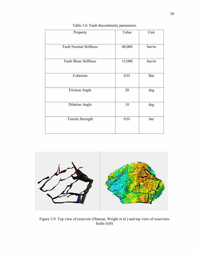
3.3.2 Defining Loading Conditions. Before the simulation runs can commence

the boundary conditions and the pressure data for each time-step is needed. A top view of

the reservoir can be seen on the right of Figure 3.9. The individual faults can be seen on

the left hand side of Figure 3.9.

Table 3.5: Reservoir grid elasticity model property ranges

Property Value Unit

Young Modulus 9.34-34.02 GPa

Poisson’s Ratio 0.23 – 0.29

Bulk Density 2.25 – 2.50 g/cm3

Biot’s Elastic Constant 1

30

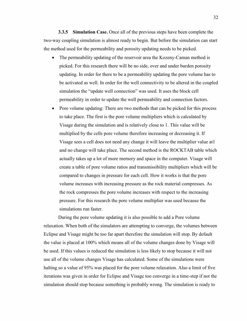
Table 3.6: Fault discontinuity parameters

Property Value Unit

Fault Normal Stiffness 40,000 bar/m

Fault Shear Stiffness 15,000 bar/m

Cohesion 0.01 Bar

Friction Angle 20 deg

Dilation Angle 10 deg

Tensile Strength 0.01 bar

Figure 3.9: Top view of reservoir (Duncan, Wright et al.) and top view of reservoirs

faults (left)

31

3.3.3 Pressure, Temperature and Water Saturation. For the two way

coupling too work accurately a pressure, temperature and water saturation is needed for

each time-step. If a time-step is missing one of these parameters it will use the previous

time-steps data. So if one time-step is missing a water saturation entry it will use the

water saturation data from the previous time-step. The range of pressure for each time-

step can be seen in Table 3.7.

In this research temperature will be omitted but water saturations will be used.

The saturation ranges are all from 0.2 to 1 during all of the time-steps. So there is no need

to display these ranges.

3.3.4 Boundary Conditions. There are three types of boundary conditions

possible which are gravity pressure, initialization and explicit initialization.

Gravity pressure: This method will simulate the initial stress using tectonic

stresses that are labeled as Sh and SH. These represent the minimum and

maximum horizontal stresses respectively. If this method is used the use of stiff

plates is recommended because pressure gradients will be used. If they are not

placed in the sideburden the pressure will not be distributed properly in the

embedded grid. The input values for this method are a Sh gradient (minimum

horizontal stress gradient), SH/Sh (Ratio of the maximum horizontal stress

gradient to minimum horizontal stress gradient), Sh azimuth (The angle that the

minimum horizontal stress creates onto a horizontal plane with respect to the

north bearing) and sea pressure gradient.

Initialization: This method will calculate the initial stress using the ratio between

the horizontal tectonic stresses and the vertical stress caused by compression. The

vertical stress is calculated using equation 6. There is an option that allows you to

add some vertical compressive stress as well. After the vertical stress is calculated

it is a matter of simple placing a Sh/Vertical and SH/vertical ratio. With this

method stiff plates in the sideburden are not required.

Explicit Initialization: This method takes a total stress property in the xx, yy, zz,

xy, yz and zx direction. Also an undefined gradient given in bar/m is needed for

each direction. This method also does need the help of stiff plates in the

sideburden.

32

3.3.5 Simulation Case. Once all of the previous steps have been complete the

two-way coupling simulation is almost ready to begin. But before the simulation can start

the method used for the permeability and porosity updating needs to be picked.

The permeability updating of the reservoir area the Kozeny-Caman method is

picked. For this research there will be no side, over and under burden porosity

updating. In order for there to be a permeability updating the pore volume has to

be activated as well. In order for the well connectivity to be altered in the coupled

simulation the “update well connection” was used. It uses the block cell

permeability in order to update the well permeability and connection factors.

Pore volume updating: There are two methods that can be picked for this process

to take place. The first is the pore volume multipliers which is calculated by

Visage during the simulation and is relatively close to 1. This value will be

multiplied by the cells pore volume therefore increasing or decreasing it. If

Visage sees a cell does not need any change it will leave the multiplier value at1

and no change will take place. The second method is the ROCKTAB table which

actually takes up a lot of more memory and space in the computer. Visage will

create a table of pore volume ratios and transmissibility multipliers which will be

compared to changes in pressure for each cell. How it works is that the pore

volume increases with increasing pressure as the rock material compresses. As

the rock compresses the pore volume increases with respect to the increasing

pressure. For this research the pore volume multiplier was used because the

simulations run faster.

During the pore volume updating it is also possible to add a Pore volume

relaxation. When both of the simulators are attempting to converge, the volumes between

Eclipse and Visage might be too far apart therefore the simulation will stop. By default

the value is placed at 100% which means all of the volume changes done by Visage will

be used. If this values is reduced the simulation is less likely to stop because it will not

use all of the volume changes Visage has calculated. Some of the simulations were

halting so a value of 95% was placed for the pore volume relaxation. Also a limit of five

iterations was given in order for Eclipse and Visage too converge in a time-step if not the

simulation should stop because something is probably wrong. The simulation is ready to

33

begin now. When running the simulation 2 processors were used for Eclipse and 6 for

Visage.

3.3.6 Running The Simulation. Once the geomechanical grid is completed and

the specifications for the case have been finished it is possible to start the simulation. The

simulations usually ran from 5 to 8 hours depending on how many iterations were needed

for convergence. A typical simulation without the geomechanical analysis took only

about thirty seconds. The increase in simulation time is due to the added calculations

Visage has to do in order to update the pore volume and permeability. When the

simulation run is finished Petrel creates a Visage file that needs to be uploaded. If the

information is loaded properly the original Eclipse simulation will be overwritten with

the two way coupling results.

34

Table 3.7: Pressure data in bar’s for each time-step

Time-step Pressure (Zhang) Time-step Pressure (Zhang)

[0] January 01 2017 173.96-224.37 [10] January 01 2027 12.08-176.77

[1] January 01 2018 23.236-176.77 [11] January 01 2028 11.40-176.77

[2] January 01 2019 22.01-176.77 [12] January 01 2029 10.77-176.77

[3] January 01 2020 20.18-176.77 [13] January 01 2030 10.19-176.77

[4] January 01 2021 18.38-176.77 [14] January 01 2031 9.67-176.77

[5] January 01 2022 16.94-176.77 [15] January 01 2032 9.21-176.77

[6] January 01 2023 15.94-176.77 [16] January 01 2033 8.81-176.77

[7] January 01 2024 14.89-176.77 [17] January 01 2034 8.42-176.77

[8] January 01 2025 13.82-176.77 [18] January 01 2035 8.06-176.77

[9] January 01 2026 12.87-176.77 [19] January 01 2036 7.74-176.77

[10] January 01 2027 12.08-176.77 [20] January 01 2037 7.47-176.77

35

4. COUPLING IN A POROUS MEDIA

When trying to understand how rock behavior or soil mechanics works one of the

simple ways to analyze them is if the model is static. When a static analysis is done the

rocks or soils are usually classified between drained or undrained (Duncan, Wright et al.

2014). When a load is applied to a drained rock liquids for example water is allowed to

enter and leave the rock. If the water is allowed to leave and enter freely the water

pressure in the pore pressure will not change due to the change in loads. But if the rock is

classified as undrained water cannot flow in or out of the rock. So if different loads are

applied during a static analysis the pressure within the pores will change as well. Since

the focus of this research is analyzing the rock behavior with respect to time intervals

things get more complicated. When the reservoir is undergoing depletion the rock/soils

will be experiencing hydraulic boundary conditions, loading and pore pressure changes.

In order to attempt to accurately simulate all of these changes happening at once the

governing equations of flow of pore fluid that goes through the rocks and the equations

relating to the rocks mass. When both problems are solved at the same time it is known as

a fully coupled simulation. In this research Petrel will be in charge of the fluid flow part

and Visage of the stress/strain analysis.

4.1 HYDRO-MECHANICAL COUPLING

The basis of hydromechanical coupling is that due to the deformation of the

geological formations the groundwater pressure is affected and its overall flow. But it is

important to note that it also works the other way around. Groundwater pressure changes

will affect how rocks will deform or fail. Petrel models this problem by defining the

effective stress as the following.

∆𝜎 = ∆𝜎′ + 𝑚 ∗ 𝛼∆𝑝 (22)

In this equation ∆σ is the total stress, ∆σ’ is the effective stress, m is a value that

becomes 1 for normal stresses and 0 for shear mechanisms. The α symbol is Biot’s

coefficient and ∆p is the change in pore pressure. It is important to note that the stress and

36

pore pressure are tension positive values. This equation is basically Terzaghis principle

with a small modification which is the addition of Biot’s coefficient. Biot’s Coefficient is

defined as:

𝛼 = 1.0 − 𝐾𝑡/𝐾𝑠 (23)

In this equation Kt is equal to the Bulk modulus of the dry rock and Ks is the Bulk

modulus of the mineral form of the rock. Since the bulk modulus is drastically smaller

than the minerals form bulk modulus the value is usually quite small. This typically

leaves Biot’s coefficient as being close to 1. Effective stress accounts for volumetric

strains caused by the compression of the rock and is defined as

∆𝜎′ = 𝐷′ ∗ ∆ε (24)

where D’ is the effective constitutive matrix which is then introduced to the equilibrium

equations.

∇𝜎 + 𝐹 = 0 (25)

In this equation F stands for the forces applied. In the model the flow of the pore

fluid is defined by Darcy’s law represented by v. The equation in order to calculate the

compressibility and continuity of the fluid is:

∇𝑇 ∗ 𝑣 − 𝑄 = (m𝑇 − m𝑇∗𝐷′

3𝐾𝑠)

𝜕ε

𝜕𝑡+ ⌊

1−φ

𝐾𝑠+

φ

𝐾𝑤−

1

(3𝐾𝑠)2 ∗ m𝑇 ∗ 𝐷′ ∗ 𝑚⌋ (𝜕p

𝜕𝑡) (26)

where φ is the porosity, t time, ε strain, Kw bulk modulus of the fluid and Q stands for

fluid flow of sources or sinks. With these equations it is possible to introduce the stress

effects into the typical reservoir simulation governing equations.

4.2 PERMEABILITY UPDATING METHOD

In order for the permeability updating two methods are possible in the software.

There are predefined functions or tables defining permeability multipliers (KM) that alter

the initial permeability (K0). In order to create an initial permeability the following

equation is used where the initial permeability is the matrix function of the permeability

for each direction.

37

Permeability is not isotropic so this step is necessary in order to acquire the

correct permeability. This formula is used for each grid block in the calculation of the

initial permeability.

𝐾0 = ⌊

𝐾𝑥 0 00 𝐾𝑦 0

0 0 𝐾𝑧

⌋ (27)

Where Kx, is the permeability in the x direction Ky permeability in y direction and

Kz permeability in z direction. These permeability reading are taken from the reservoir

simulation provided by Eclipse. The permeability multipliers are then multiplied by the

initial permeability of each cell in order to change them as the simulation progresses.

These multipliers are calculated for each time step. So the change in permeability for this

research is calculated using the Kozeny-Carman function (Carman 1956) which is

𝐾 = 𝐾0 ∗ (

𝜎03

(1+𝜎0)2

𝜎3

(1−𝜎)2

) (28)

K is the permeability for the current time-step.

4.3 POROSITY UPDATING METHOD

In a regular reservoir simulation the pore volume is modified by a single

parameter called the pore volume compressibility factor. This value is not calculated by

an equation in the software but inputted by the user after acquiring values from rock

mechanics test from the reservoir rocks. But there is another factor that has to be taken

into consideration when calculating the pore volume which is the stress changes during

the production of the reservoir. The stress behavior is calculated by Visage after each

time-step during the two way coupling simulation. Depending on the stress behavior

Visage will create a pore volume multiplier for each cell after each time-step. But if a cell

does not require a pore volume change the multiplier will be unity so that no changes are

made to that cell. This would happen if the stress and strain where not significant enough

to change the pore volume of a cell after a time-step. Some gridblocks might even suffer

an increase of porosity due to stress paths changing during the simulation run. Also

Visage will calculate the correct stress paths so pressure will be distributed accurately.

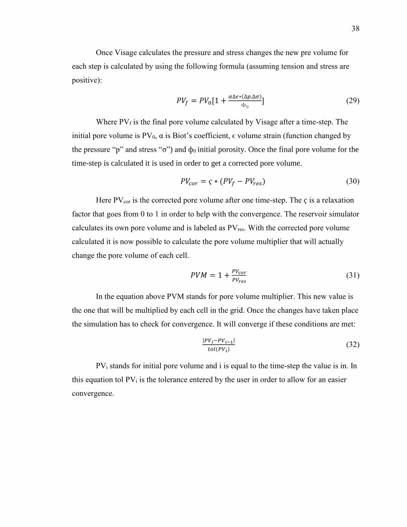
38

Once Visage calculates the pressure and stress changes the new pre volume for

each step is calculated by using the following formula (assuming tension and stress are

positive):

𝑃𝑉𝑓 = 𝑃𝑉0[1 +𝛼∆𝜖∗(∆𝑝,∆𝜎)

Φ0] (29)

Where PVf is the final pore volume calculated by Visage after a time-step. The

initial pore volume is PV0, α is Biot’s coefficient, ϵ volume strain (function changed by

the pressure “p” and stress “σ”) and ф0 initial porosity. Once the final pore volume for the

time-step is calculated it is used in order to get a corrected pore volume.

𝑃𝑉𝑐𝑜𝑟 = 𝜍 ∗ (𝑃𝑉𝑓 − 𝑃𝑉𝑟𝑒𝑠) (30)

Here PVcor is the corrected pore volume after one time-step. The 𝜍 is a relaxation

factor that goes from 0 to 1 in order to help with the convergence. The reservoir simulator

calculates its own pore volume and is labeled as PVres. With the corrected pore volume

calculated it is now possible to calculate the pore volume multiplier that will actually

change the pore volume of each cell.

𝑃𝑉𝑀 = 1 +𝑃𝑉𝑐𝑜𝑟

𝑃𝑉𝑟𝑒𝑠 (31)

In the equation above PVM stands for pore volume multiplier. This new value is

the one that will be multiplied by each cell in the grid. Once the changes have taken place

the simulation has to check for convergence. It will converge if these conditions are met:

|𝑃𝑉𝑖−𝑃𝑉𝑖−1|

𝑡𝑜𝑙(𝑃𝑉𝑖) (32)

PVi stands for initial pore volume and i is equal to the time-step the value is in. In

this equation tol PVi is the tolerance entered by the user in order to allow for an easier

convergence.

39

5. RESULTS AND DISCUSSION

Once the geomechanical grid was created the simulations could commence. The

purpose of the simulations is to show that there is a possibility of over or under

estimating the production of oil and gas. The simulations will also allow for a better

understanding of how each facies in the reservoir reacts to the reduction of permeability

due to the depletion of the reservoir. The four facies in the reservoir are sand, silt, fine silt

and clay. All the simulations will run from January 1, 2017 to January 1, 2037. During

these 20 years the time-step was placed at 1 year. So each simulation result contain 20

data points for each parameter.(Fakcharoenphol, Hu et al. 2012)

Several test simulations where conducted in order to see if during the 20 years of

production the rocks would fail and deform plastically. But with the reservoirs current

geomechanial parameters and rock physics there seemed to be no plastic deformation

after each simulation. This indicated that pore pressure coupling was not enough for the

rocks to fail .This switched the focus to mainly testing how the elastic parameters which

consisted of poisons ratio, young modulus and Biot’s coefficient altered the reservoir

performance. In order to measure the reservoir performance the cumulative oil and gas

parameters where measured for each simulation. It is also important to remember that the

reservoir contains 6 producing and 4 injector wells.

5.1 CASE 1: RESERVOIR VS TWO WAY COUPLING SIMULATION

The main point of this research is to prove that a two way coupling simulation can

deliver a more accurate representation of a reservoirs performance. Typical reservoir

simulations may be inaccurate due to the fact that only the rock compressibility factor is

used in order to model how a rock deforms and the permeability in some cases is

maintained constant during the simulation. In order to prove this point two simulations

were run. One is the regular black oil simulation done by Eclipse using the original data

from the Gullfaks reservoir model. The second simulation is the two way coupling

simulation between Eclipse and Visage. The geomechanical model created in Section 4

40

was used for this simulation since an overburden, underburden and sideburden are needed

for a successful run (Davis and Reynolds 1996). For this set of simulation no parameters

where modified, all of the actual data from the reservoir was maintained exact. The result

of both of these simulations can be seen in the following figures. In Figure 5.1 we can see

well A16 where it is possible to see that there was an oil production overestimation of

22% and gas production overestimation of 30.5%. This well had the highest production

difference between all six wells. In Figure 5.2 the cumulative gas production between

both cases is graphed.

Figure 5.1: Well A16 cumulative oil production (sm3) of regular reservoir simulation

(blue) and of coupled simulation with geomechanics included (red)

It is possible to view the oil production data for each individual well for both

simulations in Table 5.1. The next set of data Table 5.2 shows the gas production data for

each well and both simulations. The trend is that when geomechanics is added to the

simulation oil productions lower due to a decrease in permeability in all directions. The

average permeability drop was about 16 millidarcy throughout the reservoir. The

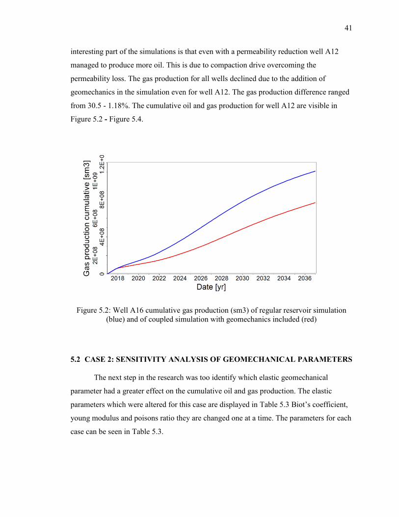
41

interesting part of the simulations is that even with a permeability reduction well A12

managed to produce more oil. This is due to compaction drive overcoming the

permeability loss. The gas production for all wells declined due to the addition of

geomechanics in the simulation even for well A12. The gas production difference ranged

from 30.5 - 1.18%. The cumulative oil and gas production for well A12 are visible in

Figure 5.2 - Figure 5.4.

Figure 5.2: Well A16 cumulative gas production (sm3) of regular reservoir simulation

(blue) and of coupled simulation with geomechanics included (red)

5.2 CASE 2: SENSITIVITY ANALYSIS OF GEOMECHANICAL PARAMETERS

The next step in the research was too identify which elastic geomechanical

parameter had a greater effect on the cumulative oil and gas production. The elastic

parameters which were altered for this case are displayed in Table 5.3 Biot’s coefficient,

young modulus and poisons ratio they are changed one at a time. The parameters for each

case can be seen in Table 5.3.

42

Table 5.1: Cumulative oil production for both simulations

Well Cum. Oil Prod. without

Geomechanics (sm^3)

Cum. Oil Prod. with

Geomechanics (sm^3)

Production

difference

A10 8.65E+05 7.88E+05 8.88%

A15 1.93E+06 1.76E+06 8.41%

A16 3.92E+06 3.053E+06 22.19%

B8 7.91E+05 7.66E+05 3.08%

B9 1.50E+06 1.44E+06 3.40%

A12 7.54E+05 8.06E+05 -6.94%

Table 5.2: Cumulative gas production for both simulations

Well Cum. Gas Prod. without

Geomechanics (sm^3)

Cum. Gas Prod. with

Geomechanics (sm^3)

Production

difference

A10 2.83E+08 2.50E+08 11.71%

A15 7.64E+08 7.07E+08 7.44%

A16 1.11E+09 7.72E+08 30.51%

B8 2.77E+08 2.71E+08 2.04%

B9 1.03E+09 1.02E+09 1.18%

A12 4.56E+08 4.04E+08 11.34%

43

Figure 5.3: Well A12 cumulative oil production (sm3) of regular reservoir simulation

(blue) and of coupled simulation with geomechanics included (red)

Figure 5.4: Well A12 cumulative gas production (sm3) of regular reservoir simulation

(blue) and of coupled simulation with geomechanics included (red)

44

Table 5.3: Min and max value for geomechanical parameters altered

Parameters Min Mid-point Max

Young Modulus 9 GPA 17 GPA 35 GPA

Poisson’s Ratio 0.23 0.27 0.29

Biot’s Coefficient 0.8 0.9 1

5.2.1 Case 2A: Young Modulus Alteration. Case 2A consisted of altering the

young modulus in order to identify how it has an effect on reservoir performance. In

order to do this the control simulation had its young modulus property modified and two

new test runs took place. These tests consisted in changing the original heterogeneous

young modulus which included an average of 17 GPA (Case Ct) into a new homogeneous

property. This new young modulus would include a homogenous distribution of 9 (Case

2A-1) and (Case 2A-2) 35 GPA. These two values where picked because they are the

minimum and maximum young modulus found in the original reservoir model. In Figure

5.5 the cumulative oil produced for well A12 is displayed in order to understand what

occurs when the young modulus is altered. In this figure three simulations are present; the

control simulation (red), control simulation with a young modulus of 9 GPA (green) and

control simulation with a young modulus of 35 GPA (black). The results for the

cumulative gas production can be viewed in Figure 5.6.. So production should lower as

the young modulus of the rocks increase, at least that was the hypothesis and logic behind

what should occur after the simulations were run and compared to the control case. From

all of the parameters this one should be the one that has a higher effect on reservoir

performance. Poisson’s ratio only states how the rock deforms in the y and x direction.

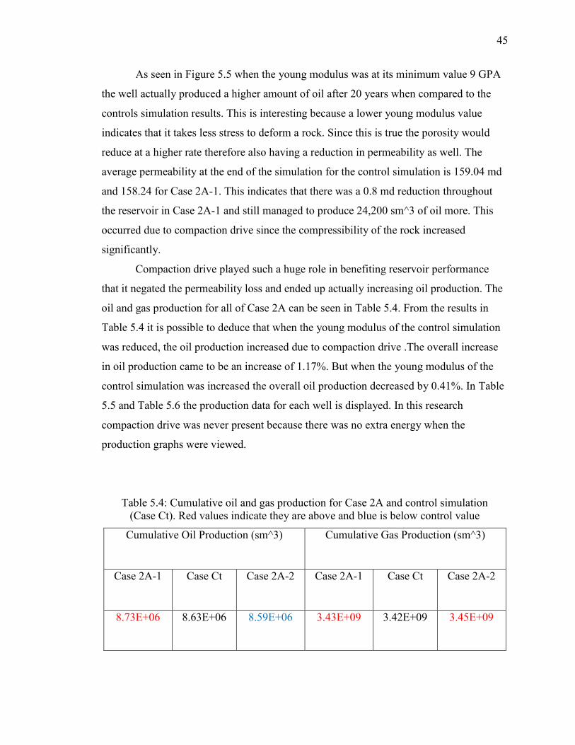
45

As seen in Figure 5.5 when the young modulus was at its minimum value 9 GPA

the well actually produced a higher amount of oil after 20 years when compared to the

controls simulation results. This is interesting because a lower young modulus value

indicates that it takes less stress to deform a rock. Since this is true the porosity would

reduce at a higher rate therefore also having a reduction in permeability as well. The

average permeability at the end of the simulation for the control simulation is 159.04 md

and 158.24 for Case 2A-1. This indicates that there was a 0.8 md reduction throughout

the reservoir in Case 2A-1 and still managed to produce 24,200 sm^3 of oil more. This

occurred due to compaction drive since the compressibility of the rock increased

significantly.

Compaction drive played such a huge role in benefiting reservoir performance

that it negated the permeability loss and ended up actually increasing oil production. The

oil and gas production for all of Case 2A can be seen in Table 5.4. From the results in

Table 5.4 it is possible to deduce that when the young modulus of the control simulation

was reduced, the oil production increased due to compaction drive .The overall increase

in oil production came to be an increase of 1.17%. But when the young modulus of the

control simulation was increased the overall oil production decreased by 0.41%. In Table

5.5 and Table 5.6 the production data for each well is displayed. In this research

compaction drive was never present because there was no extra energy when the

production graphs were viewed.

Table 5.4: Cumulative oil and gas production for Case 2A and control simulation

(Case Ct). Red values indicate they are above and blue is below control value

Cumulative Oil Production (sm^3) Cumulative Gas Production (sm^3)

Case 2A-1 Case Ct Case 2A-2 Case 2A-1 Case Ct Case 2A-2

8.73E+06 8.63E+06 8.59E+06 3.43E+09 3.42E+09 3.45E+09

46

Figure 5.5: Well A12 Cumulative oil production Young Modulus change

Figure 5.6: Well A12 Cumulative gas production Young Modulus change

47

5.2.2 Case 2B: Poisson’s Ratio Alteration. The same logic applies for the runs

in which the Poisson’s ratio are changed. Here the minimum value found in the reservoir

model was 0.23 (Case 2B-1), average 0.27 (Case Ct) and maximum 0.29 (Case 2B-1).

Using the min and max values found in the reservoir model two new runs were possible.

The cumulative oil production comparison for well A12 between the three runs can be

seen in Figure 5.7. Figure 5.8 displays the cumulative gas production is displayed for the

Poisson ratio changes.

Table 5.5: Cumulative oil production by individual well for changes in Young Modulus

Cases 2A Cumulative Oil Production (sm^3)

Wells Case 2A-1 Case Ct Case 2A-2

A10 7.96E+05 7.88E+05

7.78E+05

A15 1.78E+06

1.77E+06

1.74E+06

A16 3.08E+06

3.05E+06

3.03E+06

B8 7.80E+05

7.67E+05

8.26E+05

B9 1.47E+06

1.45E+06

1.43E+06

A12 8.30E+05

8.06E+05

7.91E+05

48

From visual inspection of Figure 5.7 and Figure 5.8 altering the Poisson ratio of

the control case had little to no effect on its reservoirs performance. There was only a

0.51% increase in oil production in Case B-1 while Case B-2 showed an oil production

reduction of 0.11%. For the gas cumulative production Case 2B-1 showed a decline in

production of 0.29% and Case B-2 had an increase of production of 0.38%. It is possible

to view the reservoirs exact production values for each case in Table 5.7. In Table 5.8 and

Table 5.9 the production data for each individual well is displayed.

Table 5.6: Cumulative gas production by individual well for changes in young modulus

Cases 2A Cumulative Gas Production (sm^3)

Wells Case 2A-1 Case Ct Case 2A-2

A10 2.50E+08

2.50E+08

2.52E+08

A15 7.06E+08

7.07E+08

7.16E+08

A16 7.76E+08

7.72E+08

7.83E+08

B8 2.71E+08

2.71E+08

2.62E+08

B9 1.01E+09

1.45E+06

1.02E+09

A12 4.14E+08

8.06E+05

4.14E+08

49

5.2.3 Case 2C: Biot’s Coefficient Alteration. For case 2C the process changed a

bit. Biot’s coefficient is assumed to be 1 in the control simulation and the original

reservoir simulation. So it is not possible to pick a min and max value. The maximum

possible value for Biot’s coefficient is 1 so two values below 1 were picked. These values

were 0.8 (Case 2C-1) and 0.9 (Case 2C-2). The logic for choosing these two values is that

0.8 is usually the minimum value placed in reservoir simulations and 0.9 is simply in-

between the other two points. The results after Biot’s coefficient change can be viewed in

Figure 5.9 and Figure 5.10. The results for Well A12 show that in Case 2C-1 there was an

increase in oil production of 2.18% and Case 2C-2 displayed a slight decrease of 0.28%.

While both showed an increase of about 1.85% and an increase of gas production of

1.86%. This is a curious finding because since Biot’s coefficient was reduced to 0.9 the

oil production lowered but if Biot’s coefficient was lowered again to 0.8 it had an

increase in oil production. The actual oil and gas produced in Case2C can be viewed at

Table 5.10. In Table 5.11 the production data for each individual well is displayedthe

production data for each individual well is displayed

5.3 CASE 3: FACIES SENSITIVITY ANALYSIS

The goal of Case 3 was to determine which facies underwent a higher

permeability loss due to the addition of geomechanics in the simulation. Only the two

simulations from Case 1 were used for this case. These are the original reservoir

simulation and the two way coupling simulation labeled (Ct). There are four facies

present in this reservoir silt, fine silt, sand and clay. The distribution of each facies can be

seen in Figure 5.11.

In order to determine the degree of permeability loss for each facies the rate of

change for each time step was determined. A total of 20 points were picked for each

facies which include the permeability in the x, y and z direction. The final permeability of

each point and time-step was an average between all directions. In order to acquire the

rate of change of permeability through each time-step the second time-step was divided

by the first permeability reading. Then the third by the second reading, these steps were

repeated for all of the time-steps.

50

All of the readings range from 0.998 to 1, the closer they are to 1 indicates that

there is less of a change between timesteps. The first rate of change from each pint was

removed because it was exaggerated since the permeability changed drastically from the

initialization step to the first year. The average rate of permeability loss for each facies

can be viewed in Figure 5.12 - Figure 5.15, each graph contains 19 data points. A

logarithmic trend line was fitted to each graph in order to acquire an enhanced idea of the

change in permeability. The facies with the highest rate of change are sand and fine silt.

5.4 CASE 4: CORRELATION ANALYSIS OF GEOMECHANICAL

PARAMETERS

This case is a correlation analysis between the elastic geomechanical parameters

chosen in case 2 and the cumulative oil/gas production. By finding the relationship

between these parameters it is possible to have an idea of how sensitive reservoir

performance is to variations in the reservoirs young modulus, Poisson ratio and Biot’s

coefficient. For this correlation analysis the control served as the middle point for each

parameter. The data set for the correlation analysis consisted of 30 data points; 15 for

cumulative oil production and 15 for cumulative gas production. In Table 5.13 it is

possible to view the values picked for the young modulus alteration and the cumulative

oil/gas production of each simulation.

Table 5.7: Cumulative oil and gas production for all Case 2B and control simulation

(Case Ct)

Cumulative Oil Production (sm^3) Cumulative Gas Production (sm^3)

Case 2B-1 Case Ct Case 2B-2 Case 2B-1 Case Ct Case 2B-2

8.67E+06 8.63E+06 8.62E+06 3.41E+09 3.42E+09 3.43E+09

51

Figure 5.7: Well A12 Cumulative oil production Poisson’s ratio change

Figure 5.8: Well A12 Cumulative gas production Poisson’s ratio change

52

Table 5.8: Cumulative oil production by individual well for changes in Poisson’s ratio

Cases 2B Cumulative Oil Production (sm^3)

Wells Case 2B-1 Case Ct Case 2B-2

A10 7.91E+05

7.88E+05

7.87E+05

A15 1.77E+06

1.77E+06

1.76E+06

A16 3.06E+06

3.05E+06

3.05E+06

B8 7.85E+05

7.67E+05

7.62E+05

B9 1.45E+06

1.45E+06

1.45E+06

A12 8.13E+05

8.06E+05

8.14E+05

Using the data from Table 5.14 - 5.16 a correlation analysis was conducted for

each parameter. The results of this study can be viewed in. All of the parameters showed

a negative correlation with respect to cumulative oil production. For the cumulative gas

production all parameters showed a negative correlation except Young modulus which

had a correlation of 0.46. This analysis tells us that whenever Young modulus, Poisson’s

ratio and Biot’s coefficient rises the cumulative oil/gas production might decrease as a

consequence. Except for the cumulative gas production for any Young modulus change

which has the opposite effect.

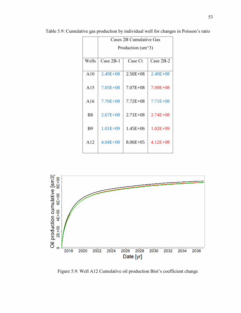
53

Table 5.9: Cumulative gas production by individual well for changes in Poisson’s ratio

Cases 2B Cumulative Gas

Production (sm^3)

Wells Case 2B-1 Case Ct Case 2B-2

A10 2.49E+08

2.50E+08

2.49E+08

A15 7.05E+08

7.07E+08

7.09E+08

A16 7.70E+08

7.72E+08

7.71E+08

B8 2.67E+08

2.71E+08

2.74E+08

B9 1.01E+09

1.45E+06

1.02E+09

A12 4.04E+08

8.06E+05

4.12E+08

Figure 5.9: Well A12 Cumulative oil production Biot’s coefficient change

54

Figure 5.10: Well A12 Cumulative gas production Biot’s coefficient change

Table 5.10: Cumulative oil and gas production for all Case 2C and control simulation

(Case Ct)

Cumulative Oil Production (sm^3) Cumulative Gas Production (sm^3)

Case 2C-1 Case Ct Case 2C-2 Case 2C-1 Case Ct Case 2C-2

8.760E+06 8.63E+06 8.57E+06

3.44E+09 3.42E+09 3.44E+09

55

Table 5.11: Cumulative oil production by individual well for changes in Biot’s

coefficient

Cases 2C Cumulative Oil Production (sm^3)

Wells Case 2C-1 Case Ct Case 2C-2

A10 7.97E+05

7.88E+05

7.83E+05

A15 1.77E+06

1.77E+06

1.76E+06

A16 3.08E+06

3.05E+06

3.04E+06

B8 7.68E+05

7.67E+05

7.50E+05

B9 1.46E+06

1.45E+06

1.44E+06

A12 8.24E+05

8.06E+05

8.04E+05

Figure 5.11: Facies distribution present in reservoir model

56

Table 5.12: Cumulative gas production by individual well for changes in Biot’s

coefficient

Cases 2C Cumulative Gas Production (sm^3)

Wells Case 2C-1 Case Ct Case 2C-2

A10 2.51E+08

2.50E+08

2.50E+08

A15 7.12E+08

7.07E+08

7.11E+08

A16 7.78E+08

7.72E+08

7.75E+08

B8 2.74E+08

2.71E+08

2.75E+08

B9 1.01E+09

1.02E+09

1.02E+09

A12 4.12E+08

4.04E+08

4.12E+08

Figure 5.12: Average permeability rate of change for sand facies

y = 0.0005ln(x) + 0.9985

0.998

0.9985

0.999

0.9995

1

0 5 10 15 20

57

Figure 5.13: Average permeability rate of change for fine silt facies

Figure 5.14: Average permeability rate of change for clay facies

y = 0.0004ln(x) + 0.9987

0.998

0.9985

0.999

0.9995

1

0 5 10 15 20

y = 0.0003ln(x) + 0.999

0.998

0.9985

0.999

0.9995

1

0 5 10 15 20

58

Figure 5.15: Average permeability rate of change for silt facies

Table 5.13: Cumulative oil and gas production for simulations with variations in its

Young Modulus

Young modulus

(GPA)

Cumulative Oil

Production (sm^3)

Cumulative Gas

Production (sm^3)

9 8.73E+06 3.43E+09

13 8.65E+06 3.42E+09

17 8.62E+06 3.43E+09

26 8.51E+06 3.45E+09

35 8.59E+06 3.43E+09

y = 0.0004ln(x) + 0.9988

0.998

0.9985

0.999

0.9995

1

0 5 10 15 20

59

Table 5.14: Cumulative oil and gas production for simulations with variations in its

Poisson’s ratio

Poisson’s Ratio Cumulative Oil

Production (sm^3)

Cumulative Gas

Production (sm^3)

0.23 8.67E+06 3.41E+09

0.25 8.64E+06 3.42E+09

0.27 8.62E+06 3.43E+09

0.28 8.60E+06 3.41E+09

0.29 8.62E+06 3.43E+09

Table 5.15: Cumulative oil and gas production for simulations with variations in its

Biot’s coefficient

Biot’s Coefficient Cumulative Oil

Production (sm^3)

Cumulative Gas

Production (sm^3)

0.8 8.70E+06 3.44E+09

0.85 8.71E+06 3.43E+09

0.9 8.57E+06 3.44E+09

0.95 8.60E+06 3.43E+09

1 8.62E+06 3.43E+09

60

Table 5.16: Correlation analysis of elastic geomechancial parameters

Correlations

Parameter Cumulative oil Production Cumulative Gas

Production

Young Modulus -0.69 0.46

Poisson’s Ratio -0.88 0.48

Biot’s Coefficient -0.69 0.65

61

6. CONCLUSION AND RECOMMENDATIONS

In this study a two way coupling simulation between Visage and Eclipse was ran.

Then its production data was compared to the typical reservoir simulation. The reservoir

simulation had a 9.6% overestimation in its cumulative oil production. There was also an

overestimation of 10.7% in its cumulative gas production. This production difference

occurred because permeability in the two way coupling was not maintained constant as in

the reservoir simulation. The two way coupling used a geomechanical analyzer in order

to correctly model the deformation of the rocks. By modeling the deformation of the rock

the porosity reduction due to the depletion of the reservoir can lead to an accurate

estimation of the permeability loss. After 20 years of production there was an overall

reduction of 16 md throughout the reservoir. This proves that for some reservoirs running

a two way coupling simulation can lead to a more accurate representation of a reservoirs

performance.

Since the research assumes that the rock deforms elastically there are only three

parameters which could have been altered in order for the sensitivity analysis. These

parameters are the reservoirs Young Modulus, Poisson’s ratio and Biot’s coefficient. The

modeling of Plastic deformation was not possible since the rock did not fail within the

allowed simulation time of 20 years. The parameter which displayed the greatest

variation on cumulative oil production was the alteration of the Young Modulus. The

total production difference was of results added to a total of 1.58%. While Biot’s

coefficient influenced cumulative gas production variation the most with 1.19%. From

the correlation analysis all of the parameters for the cumulative oil production had a

negative relationship. But for cumulative gas production altering the Young modulus had

a positive relationship while the other two parameters showed a negative relationship.

The permeability loss of each facies was also analyzed. By taking the

permeability loss variation between each time-step it was possible to view that sand and

fine silt are the ones that suffer the most during a simulation. This is due to the range of

there geomechanical parameters which implies they deform at a faster rate therefore

62

suffering a higher rate of permeability loss. If a reservoir contains a high percentage of

sand or fine silt it is recommended to run a two way coupling simulation in order to

properly model the rock deformation.

63

BIBLIOGRAPHY

Anderson, E. M. (1951). "The Dynamics of Faulting and Dyke Formation With

Applications to Britain."

Carman, P. C. (1956). Flow of gases through porous media. New York, Academic Press.

Davis, G. H. and S. J. Reynolds (1996). Structural geology of rocks and regions. New

York, John Wiley.

Doornhof, D., T. G. Kristiansen, N. B. Nagel, P. D. Pattillo and C. Sayers (2006).

"Compaction and subsidence." Oilfield Review 18(3): 50-68.

Duncan, J. M., S. G. Wright and T. L. Brandon (2014). Soil strength and slope stability.

Hoboken, New Jersey, Wiley.

Fakcharoenphol, P., L. Hu and Y.-s. Wu (2012). "Fully-Implicit Flow and Geomechanics

Model : Application for." Proceedings of the 37th Workshop on geothermal

Reservoir Engineering, Stanford.

Ingebritsen, S. E. and W. E. Sanford (1998). Groundwater in geologic processes.

Cambridge, Cambridge University Press.

Jaeger, J. C., N. G. W. Cook and R. W. Zimmerman (2007). Fundamentals of rock

mechanics. Malden, MA, Blackwell Pub.

Mohr, O. (1882). Ueber die Darstellung des Spannungszustandes und des

Deformationszustandes

eines Körperelementes und über die Anwendung derselben in der

Festigkeitslehre.

O'Connell (1994). "Geological history of the Peace River Arch in Geological Atlas of the

Western Canada Sedimentary Basin,." Canadian Society of Petroleum Geologists

and Alberta Research Council.

Settari, A. (2013). "Reservoir Compaction." Journal of Petroleum Technology 54(08):

62-69.

Terzaghi, K. (1966). Theoretical soil mechanics. New York, John Wiley.

64

Zhang, T., Bombarde, S., Strebelle, S. B., and Oatney, E. (2006). "3D porosity modeling

of a carbonate reservoir using multiple-point statistics simulation." SPE 96308,

vol. 11(3): 375-379.

Zoback, M. D. (2007). Reservoir Geomechanics. Cambridge, Cambridge University

Press.

65

VITA

Hector Gabriel Donoso was born on February 7, 1989 and received his first

Bachelor of Science in Industrial Engineering from the University of Louisville in

December 2012. He received his second Bachelor of Science in Petroleum Engineering

from Missouri University of Science and Technology in May 2014. He continued to

study at Missouri University of Science and Technology where he obtained his Master of

Science in Petroleum Engineering in December 2016.