Sensitivity of multiangle imaging to natural mixtures … of multiangle imaging to natural mixtures of aerosols over ocean Ralph Kahn, Pranab Banerjee, and Duncan McDonald Jet Propulsion

Sensitivity of multiangle imaging to natural mixturesof aerosols over ocean

Ralph Kahn, Pranab Banerjee, and Duncan McDonaldJet Propulsion Laboratory, California Institute of Technology, Pasadena

Abstract. Multiangle remote sensing data can discriminate among aerosol air mass types,as represented by climatologically probable, external mixtures of component particles.Retrievals are performed over a comparison space of four-component mixtures, selectedfrom six commonly observed components having assumed, fixed microphysical propertiesbut with mixing ratios free to vary from 0% to 100%. We refer to this approach, whichassumes climatologically probable component particles and derives aerosol mixtures fromthe observations, as a “climatological retrieval.” On the basis of simulated MultiangleImaging Spectroradiometer (MISR) observations over dark water, the retrieval candistinguish mixtures containing large, spherical particles (sea salt), nonspherical particles(accumulation and coarse mode dust), and small, dark particles (black carbon) to within20% or better of each component’s true mixing ratio. This is sufficient to distinguishmaritime from continental aerosol air masses. The retrievals, which use all nine MISRangles and the two wavelengths least affected by ocean surface reflectance (672 and 867nm), are not good at distinguishing medium, spherical, nonabsorbing (sulfate) frommedium, spherical, absorbing (carbonaceous) particles. However, the sum is retrieved towithin 20% of the true mixing ratio or better. This is significantly more detail about theproperties of particle mixtures than has previously been retrieved from satellite data, andin all cases, the derived total column aerosol optical depth remains well constrained, to atleast 0.05 or 20%, whichever is larger. We expect the MISR data, with its frequent globalcoverage, to complement in situ and field data, which can provide greater detail aboutaerosol size and composition locally. This combined effort should advance our knowledgeof aerosol behavior globally and our ability to model the impact of aerosols on theclimatically important solar radiation budget.

1. Introduction

Recent advances in modeling the Earth’s climate and study-ing its radiation balance have brought us to a point where thecontributions made by aerosols to the global radiation budgetsignificantly affect the results [e.g., Andreae, 1995; Charlson etal., 1992; Cusack et al., 1998; Hansen et al., 1997; Haywood etal., 1999; Li et al., 1997; Penner et al., 1994]. Aerosols arethought to contribute to direct radiative forcing in the atmo-sphere and indirectly through their influence as nucleationsites for cloud particles. Knowledge of both aerosol opticaldepth and microphysical properties of particles are needed toadequately model aerosol effects on climate.

Currently, we must rely on satellite remote sensing to pro-vide the spatial and temporal coverage required for globalmonitoring of atmospheric aerosols. However, the retrieval ofaerosol properties by remote sensing is a notoriously underde-termined problem, and the only operational, global-scale, sat-ellite-based retrieval of aerosols derives aerosol optical depthfrom single-angle, monospectral data, using assumed values forall the aerosol microphysical properties [Rao et al., 1989; Stoweet al., 1997].

Multiangle, multispectral remote sensing observations, suchas those anticipated from the Earth Observing System (EOS)Multiangle Imaging Spectroradiometer (MISR), provide a

type of information about the characteristics of aerosols neverbefore obtained from satellites [Martonchik et al., 1998; Dineret al., 1998a]. The instrument is unique in having higher spatialresolution, a wider range of downtrack view angles, and higherprecision onboard calibration than even the recently flownPOLDER instrument [Deschamps et al., 1994]. MISR waslaunched into polar orbit on December 18, 1999, aboard theEOS Terra satellite. It measures the upwelling shortwave ra-diance from Earth in four spectral bands, centered at 446, 558,672, and 867 nm, at each of nine view angles spread out in theforward and aft directions along the flight path at 70.58, 60.08,45.68, 26.18, and nadir. Over a period of 7 min, as the spacecraftflies overhead, a 360 km wide swath of Earth is successivelyviewed by each of the cameras. As a result, MISR samples avery large range of scattering angles, between about 608 and1608 at midlatitudes. The maximum spatial sampling rate is275 m, and global coverage is acquired about once in nine daysat the equator. The nominal mission lifetime is 6 years.

MISR data are being used to characterize surface albedoand bidirectional reflectance, and cloud properties. We alsohave algorithms to retrieve aerosol optical depth and to dis-tinguish air masses containing different mixes of atmosphericaerosols, globally.

This is the third in a series of theoretical papers that exploreour ability to retrieve information about atmospheric particlesfrom MISR. The first two papers ask how well we can distin-guish among particles having systematically and independentlyvarying ranges of microphysical properties. A four-dimensional

Copyright 2000 by the American Geophysical Union.

Paper number 2000JD900497.0148-0227/00/2000JD900497$09.00

JOURNAL OF GEOPHYSICAL RESEARCH, VOL. 106, NO. D16, PAGES 18,219–18,238, AUGUST 27, 2001

18,219

space was explored, covering natural ranges of effective size,real and imaginary refractive indexes, and optical depth [Kahnet al., 1998]. A separate investigation looked at optical depth,effective size, and spherical versus randomly oriented non-spherical shapes, for Saharan dust-like composition [Kahn etal., 1997]. The “generic” approach to aerosol retrieval, adoptedin these studies, interprets top-of-atmosphere radiances interms of a column-averaged, cross-section-weighted mean ef-fective aerosol population having unimodal, lognormal sizedistribution, and uniform composition.

On the basis of the simulations, we showed that over calmocean surfaces, and with commonly observed ranges of particleoptical depth and size distribution, the MISR algorithm canretrieve column optical depth for all but the darkest particlesto an accuracy better than 0.05 or 20%, whichever is larger,even if the microphysical properties of the particles are poorlyknown. It can distinguish spherical from nonspherical particleshaving Saharan dust-like composition. At most latitudes,MISR can also identify three to four distinct size groups be-tween 0.1 and 2.0 mm characteristic radius and two to threecompositional groups over the natural range of refractive indices.

These results indicate that the MISR aerosol retrieval candistinguish about a dozen groupings of particles over the nat-ural range of physical properties: three sizes, two or threecompositions, and spherical versus randomly oriented non-spherical particles. This represents a major improvement overcurrent operational remote sensing aerosol retrievals, suggest-ing that with MISR data, we should be able to track air masseson a global scale based on the microphysical properties of theaerosols within them.

The generic retrieval produces aerosol physical propertieswith a minimum of assumptions; of the column-average parti-cle microphysical properties, only a distribution function forparticle size, though not the characteristic radius itself, is as-sumed. This is a good approach for assessing the informationcontent of observations. However, the effective column-average particle properties obtained may not correspond toany particles actually observed in the field or predicted bytransport models. Under natural conditions, component parti-cles are mixed. Constraints on mixtures of particles in the airmass are needed to (1) identify air mass source regions, (2)track the evolution of air masses as they are advected down-stream from their sources, (3) make meaningful comparisonsbetween MISR retrievals and in situ aerosol samples, and (4)make meaningful comparisons between MISR retrievals andtransport model results.

In this paper we develop a MISR algorithm for retrievingaerosol air mass types, as represented by external mixtures ofcomponent particles. Since it is impractical to test every con-ceivable mixture of every possible component, we adopt a“climatological” retrieval approach, which asks how well wecan distinguish among mixtures of assumed, climatologicallyprobable component particles with MISR data. The additionalassumptions allow us to probe directly the way MISR mightidentify air masses containing common mixtures of aerosols inEarth’s atmosphere and to compare retrieval results with insitu observations and with aerosol transport model predictions.

Some of the best known satellite aerosol retrieval algorithmscurrently in use are climatological algorithms. These includethe advanced very high resolution radiometer (AVHRR) stan-dard retrieval [Stowe et al., 1997], and a two-channel algorithmapplied to the Ocean Color Temperature Scanner (OCTS)instrument, which flew aboard the ADEOS spacecraft [Higu-

rashi and Nakajima, 1999]. These algorithms adopt one- ortwo-component climatologies, appropriate to data from theprevious generation of remote sensing instruments but notadequate to take advantage of the additional informationabout particle properties in the MISR multiangle observations.

In section 2 we develop a climatology of four-componentmixtures, based on an analysis of published global, monthlyaerosol transport model results. This climatology is richenough to represent a range of aerosol characteristics coveringthe entire transport model data set, to at least the level ofdetail to which MISR is sensitive, based on the generic re-trieval results. We also make an effort to assess the quality ofthe climatology data, since the value of a climatological re-trieval rests on the accuracy of the assumed climatology. Sec-tion 3 describes the way we analyze the multidimensional par-ticle mixture sensitivity data. As in previous studies, weconcentrate on situations under which the MISR sensitivity toparticle properties (except possibly absorption) is likely to begreatest: over cloud-free, calm ocean. Results and conclusionsare presented in the subsequent sections.

2. An Aerosol Climatology of Four-ComponentMixtures

One of the motivations for flying MISR and other EOSinstruments is that current knowledge of the global-scale dis-tribution of aerosol air mass types is inadequate for the pur-poses of many climate change studies. However, the slate is notcompletely blank. Field observers have identified about a half-dozen broad classes of component aerosols (though their de-tailed properties vary considerably in space and time) and havediscovered that only certain combinations of components arefound commonly in nature [e.g., Prospero et al., 1983;d’Almeida et al., 1991; Kopke et al., 1997, and references there-in]. We use results from a collection of global transport models(summarized by Tegen et al. [1997]) to identify climatologicallyprobable groupings of component aerosols.

Each transport model estimates the monthly global distribu-tion of one or more of six common component aerosols: sul-fate, carbonaceous, and black carbon particles [Liousse et al.,1996], accumulation and coarse mode dust [Tegen and Fung,1995], and sea-salt particles [Tegen et al., 1997]. Some charac-teristics of these models are given in Table 1. We resampledeach model output to a uniform 18 by 18 global grid, usingbilinear interpolation. (At the 18 scale, the model results aresmooth, so resampling does not introduce spurious gradients.)For each model, the aerosol column mass per unit area wasconverted to an optical depth contribution using the factor incolumn 6 of Table 1. We linearly superposed the six dataplanes to obtain a global grid containing monthly estimates oftotal column aerosol optical depth and a fraction of total op-tical depth contributed by each of the component aerosols,evaluated at midvisible wavelengths (MISR band 2, at 558 nm).

The climatology developed in this section amounts to a newclassification of aerosol mixtures. It is aimed at meeting twoobjectives. First, it must boil the transport model results downto a small number of aerosol component groupings, which wecall mixing groups, which encompass the climatologically prob-able combinations of component aerosols for all locations andmonths. A mixing group consists of all possible fractionalamounts of four component aerosols; the microphysical prop-erties of each component are assumed and fixed, but the mix-ing ratios of each component are free to vary from 0% to

KAHN ET AL.: MULTIANGLE AEROSOL RETRIEVAL18,220

100%, in increments of 5%. This produces 1771 mixtures permixing group. We find that five mixing groups are needed tospan the climatology. In subsequent sections we test each set ofmeasurements by comparing it with all mixtures in all fivemixing groups, for each of 21 values of column aerosol opticaldepth, a total of 185,955 comparison models.

The second goal of the climatology is to identify air masstypes, composed of specific fractional amounts of componentparticles in the mixing groups, which give a fair representationof the global-scale spatial and temporal aerosol mixture pat-terns. These representative air mass types are not needed forclimatological retrievals with MISR data, but for the sensitivitystudy, they are used to generate sample measurements. Thesensitivity study asks how narrow a range of mixtures, fromamong all those in the entire comparison space, give accept-able matches to the simulated MISR radiances in each set ofsample measurements. A narrower range indicates that theretrieval is more specific as to the identity and fraction of eachcomponent present.

2.1. Mixture Classification

We begin by defining mixing groups as combinations ofcomponent particles in the aerosol climatology. We expectMISR to make about a dozen distinctions based on aerosolmicrophysical properties [Kahn et al., 1998, 1997]. This amountof detail is captured by mixtures of four component aerosols;having fewer components would eliminate some climatologi-cally common mixtures that MISR can identify, whereas in-cluding more components adds only redundant retrieval re-sults. So we classify the six-layer, aggregated, global transportmodel data set according to the four component particles thatcontribute most to the total column optical depth at eachlocation and month. The two components that contribute leastto a given space-time grid cell are ignored for that cell.

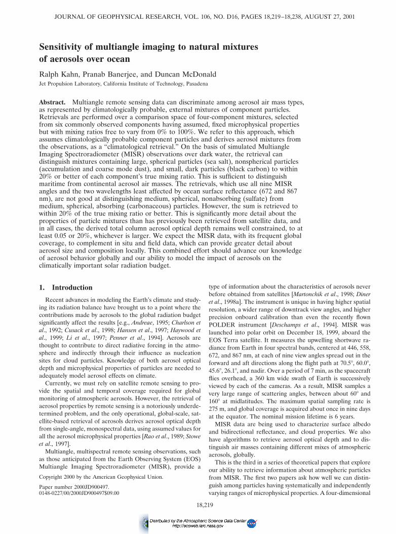
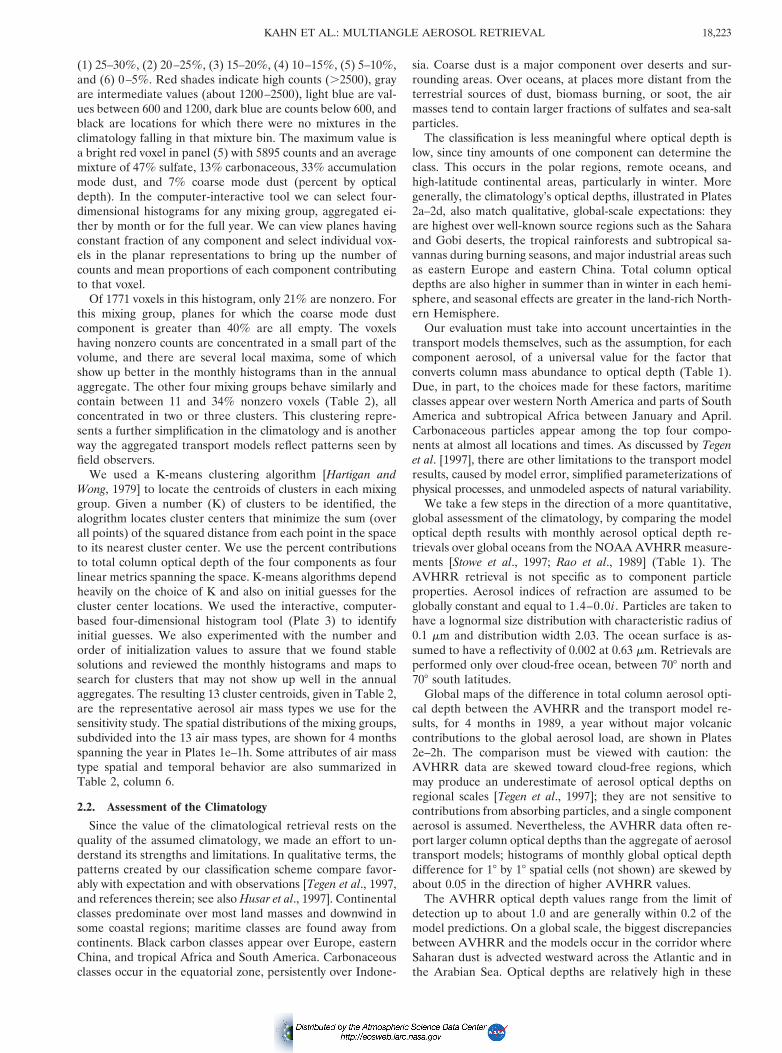
Plates 1a–1d give maps of particle mixing groups for 4months spanning the year. The corresponding total columnoptical depths, also derived from the aggregated transportmodel results, are shown in Plates 2a–2d. Although the modelresults for most aerosol components were developed indepen-dently of each other, the mixture data are highly clustered. Ofthe 15 possible combinations of four component particles thatcan be made from the six included in the climatology, only fivecombinations are needed to describe the top four componentsfor nearly the entire data set. This is an enormous simplifica-tion, indicating that in at least one respect, the aggregatedtransport models reflect aerosol mixture patterns noted by fieldobservers. These mixing groups meet the first objective of theclimatology, to provide a broad comparison space. Their com-positions are given as major headings in Table 2.

All five mixing groups contain sulfate particles. We label as“maritime” those groups that contain sea-salt particles; we call“continental” those groups that do not have sea salt among thefour most abundant component particles but do have accumu-lation mode dust. The other aerosol components contributingto each group determine whether the classification is “dusty,”“carbonaceous,” or “black carbon.” Representative colors forthe maps in Plate 1 are chosen so that the most commonmaritime classes appear in shades of blue; the most commoncontinental classes are brown. For those that remain, classesrich in black carbon are gray, those having high carbonaceousaerosol fraction are green, and the ones abundant in coarsedust are yellow.

We now address the second objective of the climatology, toTab

le1.

Mon

thly

,Glo

balA

eros

olT

rans

port

Mod

els

Use

din

Thi

sSt

udy

Com

pone

ntA

eros

olSo

urce

Ref

eren

ceSp

atia

lRes

olut

ion

Qua

ntiti

esR

epor

ted

Uni

tsG

iven

Fac

tor

Use

dto

Con

vert

Col

umn

Mas

spe

rA

rea

tot

Acc

umul

atio

nan

dco

arse

min

eral

dust

*G

ISS

Teg

enan

dF

ung

[199

5]48

358

tota

lcol

umn

dust

optic

alde

pth,

regr

oupe

din

to2

size

bins

:,1

mm

(acc

umul

atio

n),1

–10

mm

(coa

rse)

none

1.5

m2

g21

(acc

umul

atio

nm

ode)

;0.

33

m2

g21

(coa

rse

mod

e)

Sea

salt*

GIS

ST

egen

etal

.[19

97]

483

58to

talc

olum

nae

roso

lopt

ical

thic

knes

sno

ne0.

3m

2g2

1

Sulfa

tes†

LL

NL

Lio

usse

etal

.[19

96]

;4.

583

7.58

colu

mn

mas

slo

adg

m2

28.

5m

2g2

1

Car

bona

ceou

spa

rtic

les*

GIS

SL

ious

seet

al.[

1996

]48

358

tota

lcol

umn

aero

solo

ptic

alth

ickn

ess

none

8.0

m2

g21

Bla

ckca

rbon

*G

ISS

Lio

usse

etal

.[19

96]

483

58to

talc

olum

nae

roso

lopt

ical

thic

knes

sno

ne9.

m2

g21

Tot

alae

roso

l‡(a

ssum

es“s

ulfa

te”

optic

alpr

oper

ties)

NO

AA

/AV

HR

RSt

owe

etal

.[19

97]

183

18gl

obal

ocea

ns1

708

to2

708

latit

ude

tota

lcol

umn

optic

alde

pth

(at

0.63

mm

)no

neop

tical

dept

had

just

men

tap

plie

dt9

51.

56t

10.

03

Sulfa

tes*

GIS

SC

hin

etal

.[19

96]

483

58to

talc

olum

nae

roso

lopt

ical

thic

knes

sno

ne6.

0m

2g2

1(l

and)

10m

2g2

1(o

cean

)

*Dat

aob

tain

edfr

omT

egen

etal

.[19

97],

God

dard

Inst

itute

ofSp

ace

Stud

ies

(web

site

(htt

p://w

ww

.gis

s.na

sa.g

ov/g

acp/

tran

spor

t/)19

97.

†Obt

aine

dfr

omJ.

Penn

eret

al.,

from

the

Law

renc

eL

iver

mor

eN

atio

nalL

abor

ator

y(L

LN

L)

mod

el,p

erso

nalc

omm

unic

atio

n,19

98.

‡Obt

aine

dfr

omL

.Sto

we

etal

.,N

atio

nalO

cean

ogra

phic

and

Atm

osph

eric

Adm

inis

trat

ion

(NO

AA

),pe

rson

alco

mm

unic

atio

n,19

97.

18,221KAHN ET AL.: MULTIANGLE AEROSOL RETRIEVAL

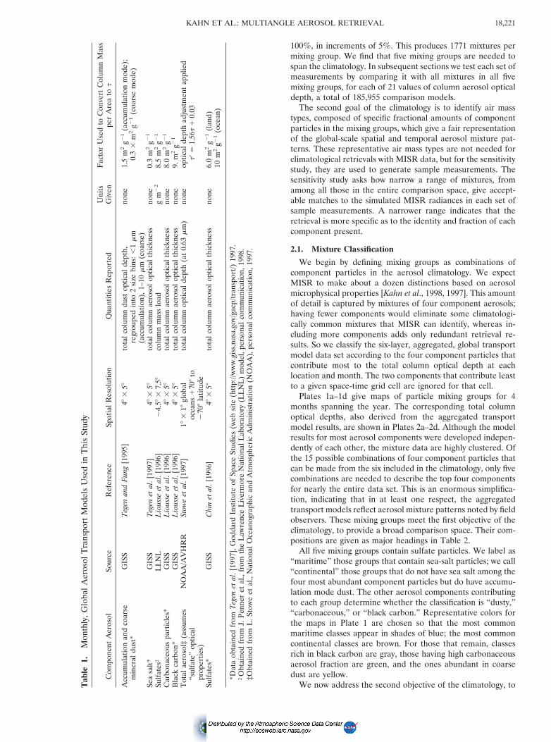
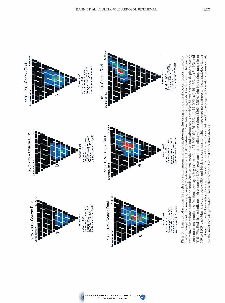
identify representative air mass types having specific fractionalamounts of component particles, to be used as sample atmo-spheres in the sensitivity study. Plate 3 illustrates that theactual proportions of the four components within each groupare also highly clustered in the transport model results. Thisplate shows slices through a four-dimensional histogram of theaerosol components for the “carbonaceous 1 dusty continen-tal” mixing group, aggregated over the year. The full diagramis a tetrahedron, divided into voxels that correspond to mix-tures having different proportions of each of the four compo-nent particles (in this case: sulfate, accumulation mode dust,coarse mode dust, and carbonaceous particles). Vertices of thetetrahedron represent 100% of a component, and along the

edges are mixtures of only two components. Each triangularfacet is a standard ternary mixing diagram; in the facet interiorare three-component mixtures of systematically varying pro-portions. Points interior to the tetrahedron volume correspondto four-component mixtures. For this four-dimensional histo-gram we have chosen a 5% increment. The voxel at one of thevertices of the tetrahedron is colored according to the numberof occurrences in the climatology of a mixture with 100% of thecomponent aerosol associated with that vertex, immediatelyadjacent voxels have at least 95% but less than 100% of thatcomponent, etc.

Plate 3 shows six planes having constant coarse mode dustfraction, corresponding to bins containing coarse mode dust of

Table 2. Climatological Mixing Groups and Representative Air Mass Types

Classification Component 1 Component 2 Component 3 Component 4 Notes

1. Carbonaceous 1dusty maritime

sulfate sea salt carbonaceous accum. dust 34% of voxels are nonzero

1a (0.67) 0.13 0.10 0.10 middle- to high-latitude oceans, winter; Nov.–May, southern oceans; May–Sept., NorthAtlantic

1b 0.41 0.13 (0.27) (0.19) tropical to subtropical oceans, all year; June–Oct., remote southern oceans

1c 0.40 (0.32) 0.17 0.11 southern midlatitude oceans, all year; Nov.–March, remote southern oceans

2. Dusty maritime 1coarse dust

sulfate sea salt accum. dust coarse dust 14% of voxels are nonzero

2a (0.52) 0.17 0.21 0.10 downwind of deserts: Australia, Africa, SouthAmerica, peak during southern summer;Oct.–Jan., N. W. Africa

2b 0.29 0.13 (0.39) (0.19) same pattern as 2a but closer to continentalsource regions

3. Carbonaceous 1black carbon maritime

sulfate sea salt carbonaceous black carbon 11% of voxels are nonzero

3a (0.51) 0.18 0.26 0.05 ocean near Indonesia, all year; Dec.–March,North Atlantic; Jan.–Feb., oceans nearcentral Africa; May–July, oceans neartropical South America; July–Sept., oceansnear central America

3b 0.35 0.10 (0.47) (0.08) same pattern as 3a but closer to continentalsource regions

4. Carbonaceous 1dusty continental

sulfate accum. dust coarse dust carbonaceous 21% of voxels are nonzero

4a (0.61) 0.21 0.05 0.13 Feb.–Nov., eastern North America;July–Sept., western North America; Jan.–March, South America; Jan.–March,southern Africa; Oct., India; July–Oct.,Korea

4b 0.40 (0.35) 0.09 (0.16) March–July, Oct.–Nov., western NorthAmerica; Sept.–Dec., South America;April–Oct., S. Africa; Jan.–March, centralAsia; April–June, Nov.–Dec., Korea

4c 0.22 (0.51) (0.16) 0.11 Arabia and North Africa, all year; Nov.–Dec.,S. Africa; March–Dec., central Asia; Jan.–April, July–Dec., Australia

5. Carbonaceous 1black carbon continental

sulfate accum. dust carbonaceous black carbon 15% of voxels are nonzero

5a (0.59) 0.12 0.23 0.06 April–Oct., Europe; Jan.–March, north Asia;July–Sept., east China; Nov.–March, eastNorth America; Nov.–March, equatorialSouth America

5b 0.25 0.12 (0.54) 0.09 Tropical-subtropical Africa, all year; Dec.–March, west Europe; Jan.–March, northAsia; Jan.–March, east China

5c 0.44 (0.23) (0.26) 0.07 Nov.–Jan., west Europe; Oct.–March, eastEurope; Nov.–Feb., north Asia; Oct.–Dec.,April–July, east China; Dec.–April,equatorial South America

Relative abundances are given as fractions of the total optical depth in MISR band 2 (558 nm effective wavelength). Numbers in parenthesesare distinctive constituents of the mixture. “Accum. dust” stands for accumulation mode dust.


(1) 25–30%, (2) 20–25%, (3) 15–20%, (4) 10–15%, (5) 5–10%,and (6) 0–5%. Red shades indicate high counts (.2500), grayare intermediate values (about 1200–2500), light blue are val-ues between 600 and 1200, dark blue are counts below 600, andblack are locations for which there were no mixtures in theclimatology falling in that mixture bin. The maximum value isa bright red voxel in panel (5) with 5895 counts and an averagemixture of 47% sulfate, 13% carbonaceous, 33% accumulationmode dust, and 7% coarse mode dust (percent by opticaldepth). In the computer-interactive tool we can select four-dimensional histograms for any mixing group, aggregated ei-ther by month or for the full year. We can view planes havingconstant fraction of any component and select individual vox-els in the planar representations to bring up the number ofcounts and mean proportions of each component contributingto that voxel.

Of 1771 voxels in this histogram, only 21% are nonzero. Forthis mixing group, planes for which the coarse mode dustcomponent is greater than 40% are all empty. The voxelshaving nonzero counts are concentrated in a small part of thevolume, and there are several local maxima, some of whichshow up better in the monthly histograms than in the annualaggregate. The other four mixing groups behave similarly andcontain between 11 and 34% nonzero voxels (Table 2), allconcentrated in two or three clusters. This clustering repre-sents a further simplification in the climatology and is anotherway the aggregated transport models reflect patterns seen byfield observers.

We used a K-means clustering algorithm [Hartigan andWong, 1979] to locate the centroids of clusters in each mixinggroup. Given a number (K) of clusters to be identified, thealogrithm locates cluster centers that minimize the sum (overall points) of the squared distance from each point in the spaceto its nearest cluster center. We use the percent contributionsto total column optical depth of the four components as fourlinear metrics spanning the space. K-means algorithms dependheavily on the choice of K and also on initial guesses for thecluster center locations. We used the interactive, computer-based four-dimensional histogram tool (Plate 3) to identifyinitial guesses. We also experimented with the number andorder of initialization values to assure that we found stablesolutions and reviewed the monthly histograms and maps tosearch for clusters that may not show up well in the annualaggregates. The resulting 13 cluster centroids, given in Table 2,are the representative aerosol air mass types we use for thesensitivity study. The spatial distributions of the mixing groups,subdivided into the 13 air mass types, are shown for 4 monthsspanning the year in Plates 1e–1h. Some attributes of air masstype spatial and temporal behavior are also summarized inTable 2, column 6.

2.2. Assessment of the Climatology

Since the value of the climatological retrieval rests on thequality of the assumed climatology, we made an effort to un-derstand its strengths and limitations. In qualitative terms, thepatterns created by our classification scheme compare favor-ably with expectation and with observations [Tegen et al., 1997,and references therein; see also Husar et al., 1997]. Continentalclasses predominate over most land masses and downwind insome coastal regions; maritime classes are found away fromcontinents. Black carbon classes appear over Europe, easternChina, and tropical Africa and South America. Carbonaceousclasses occur in the equatorial zone, persistently over Indone-

sia. Coarse dust is a major component over deserts and sur-rounding areas. Over oceans, at places more distant from theterrestrial sources of dust, biomass burning, or soot, the airmasses tend to contain larger fractions of sulfates and sea-saltparticles.

The classification is less meaningful where optical depth islow, since tiny amounts of one component can determine theclass. This occurs in the polar regions, remote oceans, andhigh-latitude continental areas, particularly in winter. Moregenerally, the climatology’s optical depths, illustrated in Plates2a–2d, also match qualitative, global-scale expectations: theyare highest over well-known source regions such as the Saharaand Gobi deserts, the tropical rainforests and subtropical sa-vannas during burning seasons, and major industrial areas suchas eastern Europe and eastern China. Total column opticaldepths are also higher in summer than in winter in each hemi-sphere, and seasonal effects are greater in the land-rich North-ern Hemisphere.

Our evaluation must take into account uncertainties in thetransport models themselves, such as the assumption, for eachcomponent aerosol, of a universal value for the factor thatconverts column mass abundance to optical depth (Table 1).Due, in part, to the choices made for these factors, maritimeclasses appear over western North America and parts of SouthAmerica and subtropical Africa between January and April.Carbonaceous particles appear among the top four compo-nents at almost all locations and times. As discussed by Tegenet al. [1997], there are other limitations to the transport modelresults, caused by model error, simplified parameterizations ofphysical processes, and unmodeled aspects of natural variability.

We take a few steps in the direction of a more quantitative,global assessment of the climatology, by comparing the modeloptical depth results with monthly aerosol optical depth re-trievals over global oceans from the NOAA AVHRR measure-ments [Stowe et al., 1997; Rao et al., 1989] (Table 1). TheAVHRR retrieval is not specific as to component particleproperties. Aerosol indices of refraction are assumed to beglobally constant and equal to 1.4–0.0i . Particles are taken tohave a lognormal size distribution with characteristic radius of0.1 mm and distribution width 2.03. The ocean surface is as-sumed to have a reflectivity of 0.002 at 0.63 mm. Retrievals areperformed only over cloud-free ocean, between 708 north and708 south latitudes.

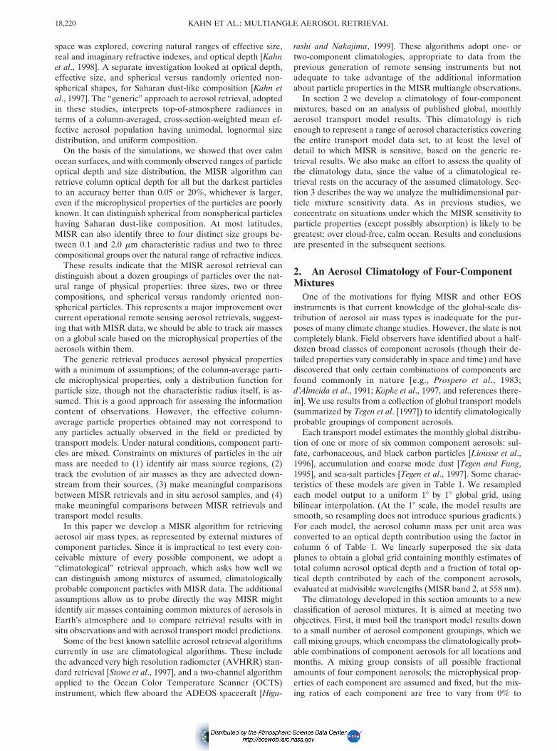
Global maps of the difference in total column aerosol opti-cal depth between the AVHRR and the transport model re-sults, for 4 months in 1989, a year without major volcaniccontributions to the global aerosol load, are shown in Plates2e–2h. The comparison must be viewed with caution: theAVHRR data are skewed toward cloud-free regions, whichmay produce an underestimate of aerosol optical depths onregional scales [Tegen et al., 1997]; they are not sensitive tocontributions from absorbing particles, and a single componentaerosol is assumed. Nevertheless, the AVHRR data often re-port larger column optical depths than the aggregate of aerosoltransport models; histograms of monthly global optical depthdifference for 18 by 18 spatial cells (not shown) are skewed byabout 0.05 in the direction of higher AVHRR values.

The AVHRR optical depth values range from the limit ofdetection up to about 1.0 and are generally within 0.2 of themodel predictions. On a global scale, the biggest discrepanciesbetween AVHRR and the models occur in the corridor whereSaharan dust is advected westward across the Atlantic and inthe Arabian Sea. Optical depths are relatively high in these


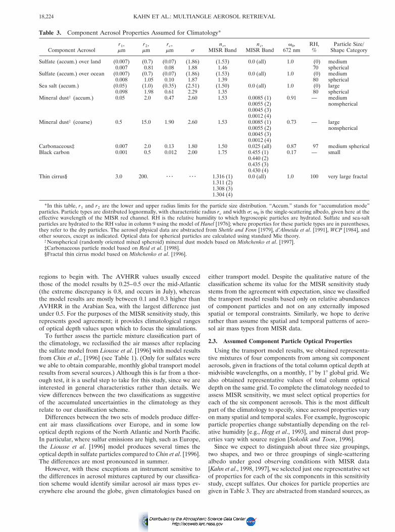
regions to begin with. The AVHRR values usually exceedthose of the model results by 0.25–0.5 over the mid-Atlantic(the extreme discrepancy is 0.8, and occurs in July), whereasthe model results are mostly between 0.1 and 0.3 higher thanAVHRR in the Arabian Sea, with the largest difference justunder 0.5. For the purposes of the MISR sensitivity study, thisrepresents good agreement; it provides climatological rangesof optical depth values upon which to focus the simulations.

To further assess the particle mixture classification part ofthe climatology, we reclassified the air masses after replacingthe sulfate model from Liousse et al. [1996] with model resultsfrom Chin et al., [1996] (see Table 1). (Only for sulfates werewe able to obtain comparable, monthly global transport modelresults from several sources.) Although this is far from a thor-ough test, it is a useful step to take for this study, since we areinterested in general characteristics rather than details. Weview differences between the two classifications as suggestiveof the accumulated uncertainties in the climatology as theyrelate to our classification scheme.

Differences between the two sets of models produce differ-ent air mass classifications over Europe, and in some lowoptical depth regions of the North Atlantic and North Pacific.In particular, where sulfur emissions are high, such as Europe,the Liousse et al. [1996] model produces several times theoptical depth in sulfate particles compared to Chin et al. [1996].The differences are most pronounced in summer.

However, with these exceptions an instrument sensitive tothe differences in aerosol mixtures captured by our classifica-tion scheme would identify similar aerosol air mass types ev-erywhere else around the globe, given climatologies based on

either transport model. Despite the qualitative nature of theclassification scheme its value for the MISR sensitivity studystems from the agreement with expectation, since we classifiedthe transport model results based only on relative abundancesof component particles and not on any externally imposedspatial or temporal constraints. Similarly, we hope to deriverather than assume the spatial and temporal patterns of aero-sol air mass types from MISR data.

2.3. Assumed Component Particle Optical Properties

Using the transport model results, we obtained representa-tive mixtures of four components from among six componentaerosols, given in fractions of the total column optical depth atmidvisible wavelengths, on a monthly, 18 by 18 global grid. Wealso obtained representative values of total column opticaldepth on the same grid. To complete the climatology needed toassess MISR sensitivity, we must select optical properties foreach of the six component aerosols. This is the most difficultpart of the climatology to specify, since aerosol properties varyon many spatial and temporal scales. For example, hygroscopicparticle properties change substantially depending on the rel-ative humidity [e.g., Hegg et al., 1993], and mineral dust prop-erties vary with source region [Sokolik and Toon, 1996].

Since we expect to distinguish about three size groupings,two shapes, and two or three groupings of single-scatteringalbedo under good observing conditions with MISR data[Kahn et al., 1998, 1997], we selected just one representative setof properties for each of the six components in this sensitivitystudy, except sulfates. Our choices for particle properties aregiven in Table 3. They are abstracted from standard sources, as

Table 3. Component Aerosol Properties Assumed for Climatology*

Component Aerosolr1,mm

r2,mm

rc,mm s

nr,MISR Band

ni,MISR Band

v0,672 nm

RH,%

Particle Size/Shape Category

Sulfate (accum.) over land (0.007) (0.7) (0.07) (1.86) (1.53) 0.0 (all) 1.0 (0) medium0.007 0.81 0.08 1.88 1.46 70 spherical

Sulfate (accum.) over ocean (0.007) (0.7) (0.07) (1.86) (1.53) 0.0 (all) 1.0 (0) medium0.008 1.05 0.10 1.87 1.39 80 spherical

Sea salt (accum.) (0.05) (1.0) (0.35) (2.51) (1.50) 0.0 (all) 1.0 (0) large0.098 1.98 0.61 2.29 1.35 80 spherical

Mineral dust† (accum.) 0.05 2.0 0.47 2.60 1.53 0.0085 (1) 0.91 — medium0.0055 (2) nonspherical0.0045 (3)0.0012 (4)

Mineral dust† (coarse) 0.5 15.0 1.90 2.60 1.53 0.0085 (1) 0.73 — large0.0055 (2) nonspherical0.0045 (3)0.0012 (4)

Carbonaceous‡ 0.007 2.0 0.13 1.80 1.50 0.025 (all) 0.87 97 medium sphericalBlack carbon 0.001 0.5 0.012 2.00 1.75 0.455 (1) 0.17 — small

0.440 (2)0.435 (3)0.430 (4)

Thin cirrus§ 3.0 200. z z z z z z 1.316 (1) 0.0 (all) 1.0 100 very large fractal1.311 (2)1.308 (3)1.304 (4)

*In this table, r1 and r2 are the lower and upper radius limits for the particle size distribution. “Accum.” stands for “accumulation mode”particles. Particle types are distributed lognormally, with characteristic radius rc and width s; v0 is the single-scattering albedo, given here at theeffective wavelength of the MISR red channel. RH is the relative humidity to which hygroscopic particles are hydrated. Sulfate and sea-saltparticles are hydrated to the RH value in column 9 using the model of Hanel [1976]; where properties for these particle types are in parentheses,they refer to the dry particles. The aerosol physical data are abstracted from Shettle and Fenn [1979], d’Almeida et al. [1991], WCP [1984], andother sources, except as indicated. Optical data for spherical particles are calculated using standard Mie theory.

†Nonspherical (randomly oriented mixed spheroid) mineral dust models based on Mishchenko et al. [1997].‡Carbonaceous particle model based on Reid et al. [1998].§Fractal thin cirrus model based on Mishchenko et al. [1996].


Plate 1. (a–d) Global maps for January, April, July, and October, respectively, showing the spatial distri-bution of the five aerosol mixing groups defined as major headings in Table 2, based on the aggregate ofaerosol transport models listed in Table 1. (e–h) Global maps for January, April, July, and October, respec-tively, showing the spatial distribution of the 13 representative air mass types, defined in Table 2. To obtainthese maps, each point was first classified by aerosol mixing group and then subclassified according to therepresentative air mass type nearest it, using percent contributions to total column optical depth of eachcomponent as the four-dimensional, linear distance metric.


Plate 2. (a–d) Global maps of total column aerosol optical depth (“tau”) for January, April, July, andOctober, respectively, derived from the transport models of Tegen et al. [1997]. (e–h) Difference mapsbetween AVHRR-retrieved total column aerosol optical depth for 1989 [Stowe et al., 1997] and the corre-sponding monthly transport model results for January, April, July, and October, respectively. The blue regionsindicate places where no AVHRR data exist.


Pla

te3.

Exa

mpl

eof

sect

ions

thro

ugh

afo

ur-d

imen

sion

alhi

stog

ram

,sho

win

gcl

uste

ring

inth

ecl

imat

olog

ical

prop

ortio

nsof

the

aero

solc

ompo

nent

sfo

rm

ixin

ggr

oup

4(“

carb

onac

eous

1du

sty

cont

inen

tal”

inT

able

2),a

ggre

gate

dov

era

year

.Thi

sm

ixin

ggr

oup

incl

udes

sulfa

te,a

ccum

ulat

ion

mod

edu

st,c

oars

em

ode

dust

,and

carb

onac

eous

part

icle

s.Sh

own

here

are

six

plan

esha

ving

cons

tant

coar

sem

ode

dust

frac

tion,

corr

espo

ndin

gto

bins

of(a

)25

–30%

,(b)

20–2

5%,(

c)15

–20%

,(d)

10–1

5%,(

e)5–

10%

,and

(f)0

–5%

.Red

shad

esin

dica

tehi

ghco

unts

(.25

00),

gray

are

inte

rmed

iate

valu

es(a

bout

1200

–250

0),l

ight

blue

valu

esra

nge

from

600

to12

00,d

ark

blue

are

coun

tsbe

low

600,

and

blac

kar

elo

catio

nsfo

rw

hich

ther

ew

ere

nom

ixtu

res

inth

ecl

imat

olog

yfa

lling

inth

atm

ixtu

rebi

n.B

elow

each

sect

ion

are

num

eric

alva

lues

ofth

enu

mbe

rof

hits

,and

the

aver

age

frac

tion

ofea

chco

mpo

nent

,fo

rth

em

ost

heav

ilypo

pula

ted

pixe

lin

that

sect

ion.

See

text

for

furt

her

deta

ils.


referenced in this table.We hydrated the sulfate particles to equilibrium at 70%

relative humidity for “continental” air mass types and to 80%for “maritime” air masses using the hydration model of Hanel[1976]. We also defined two vertical distributions for accumu-lation mode dust; one, used for “continental” air mass types,places all the dust in a near-surface layer, as we do for all othercomponents. The second, used for “maritime” air masses tosimulate dust particles transported far from their source re-gions, distributes the particles between 5 and 10 km above thesurface, with a scale height of 10 km. We used a Mie algorithmto relate physical to optical properties for the spherical parti-cles; for nonspherical dust and cirrus, we obtained T-matrixresults from Mishchenko et al. [1996, 1997; personal commu-nication, 2000]. Extinction and scattering properties for distri-butions of particles are calculated as weighted averages. Thelognormal size distribution used is

dN~r!dr 5

1

r ln ~s! Î2pexp F2

~ln ~r! 2 ln ~rc!!2

2~ln ~s!2! G . (1)

The width parameter (s) and characteristic radius (rc) foreach case are given in Table 3, and N(r) is the number densityof particles at radius (r).

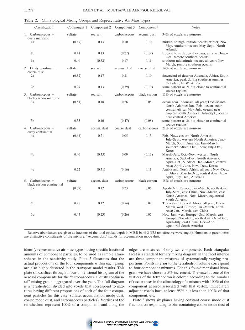
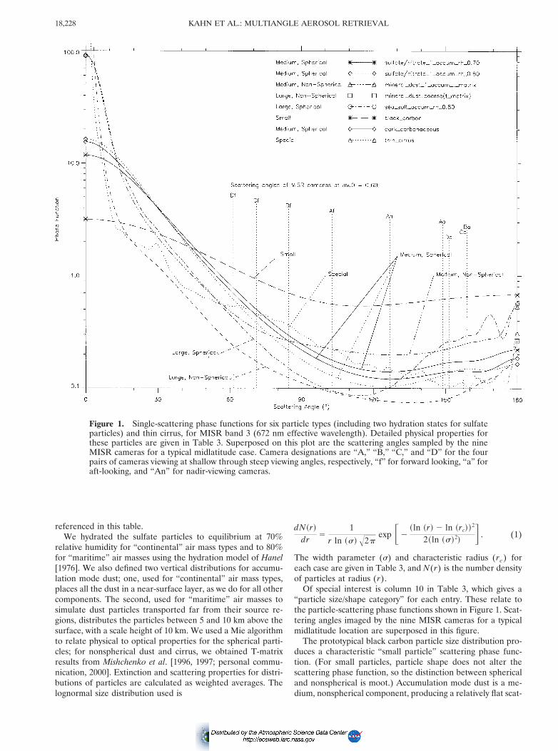
Of special interest is column 10 in Table 3, which gives a“particle size/shape category” for each entry. These relate tothe particle-scattering phase functions shown in Figure 1. Scat-tering angles imaged by the nine MISR cameras for a typicalmidlatitude location are superposed in this figure.

The prototypical black carbon particle size distribution pro-duces a characteristic “small particle” scattering phase func-tion. (For small particles, particle shape does not alter thescattering phase function, so the distinction between sphericaland nonspherical is moot.) Accumulation mode dust is a me-dium, nonspherical component, producing a relatively flat scat-

Figure 1. Single-scattering phase functions for six particle types (including two hydration states for sulfateparticles) and thin cirrus, for MISR band 3 (672 nm effective wavelength). Detailed physical properties forthese particles are given in Table 3. Superposed on this plot are the scattering angles sampled by the nineMISR cameras for a typical midlatitude case. Camera designations are “A,” “B,” “C,” and “D” for the fourpairs of cameras viewing at shallow through steep viewing angles, respectively, “f” for forward looking, “a” foraft-looking, and “An” for nadir-viewing cameras.


tering phase function between a 708 and 1608 scattering angle.Carbonaceous particles, as well as the two sulfate components,are categorized as medium, spherical. The coarse mode dustand sea salt are large, nonspherical and large, spherical particletypes, respectively. Each has a steeply sloped scattering phasefunction at small scattering angles. The thin cirrus model pro-duces a scattering phase function distinct from the other com-ponent aerosols. We also expect to distinguish absorbing(“dirty”) from nonabsorbing (“clean”) particles. In Table 3 thedust, carbonaceous, and black carbon particles are absorbing.It is on the basis of these differences among particle scatteringphase functions and absorption characteristics that we expectto discriminate among natural mixtures of particles with MISRdata.

3. Our Approach to the Aerosol MixtureSensitivity Study

Our approach to the climatological sensitivity study is similarto that adopted by Kahn et al. [1998] for the generic retrievalstudy. We use simulations of top-of-atmosphere radiation toexplore the sensitivity of multiangle observations to aerosolproperties. The MISR Team has developed a radiative transfercode, based on the matrix operator method [Grant and Hunt,1968]. It simulates reflectances as would be observed by MISRfor arbitrary choice of aerosol mixture, amount, and verticaldistribution, variable surface reflectance properties, and user-selected Sun and viewing geometry [Diner et al., 1998a]. Radi-ances for mixtures of aerosol components are obtained bycombining radiances for the individual components, weightedby their fractional contribution to optical depth, according tothe modified linear mixing method of Abdou et al. [1997]. Forthe present study we simulated MISR measurements over aFresnel-reflecting flat ocean surface, in a cloud-free, Rayleigh-scattering atmosphere with a surface pressure of 1.013 bar, astandard midlatitude temperature profile, and aerosols (excepttransported accumulation mode dust) concentrated in a near-surface layer.

We assume here that the vertical distribution of aerosols hasa negligible effect on the results. Our tests with particles insideand above the Rayleigh scattering layer show that the effectmay be significant, particularly at the blue and green wave-lengths and at the steepest viewing angles. However, mostatmospheric aerosols are concentrated near the surface, andthe MISR dark water retrievals use only the red and infraredchannels, for which Rayleigh scattering is small. Other particlemodels will be added as needed when we are analyzing MISRdata, particularly when we have the benefit of detailed fieldmeasurements at the observation site. For MISR retrievalsover ocean we also model Sun glint and whitecaps, whichdepend on near-surface wind speed [Martonchik et al., 1998],and of course, we anticipate modifying the MISR retrievalalgorithm, as needed, as we gain experience working withspacecraft data.

We designate one set of simulated reflectances as the MISR“measurements.” For a measurement the atmosphere has afixed total aerosol optical depth and specified fractional con-tributions from each of four component particles. We then testwhether the measured radiances can be distinguished, withininstrument uncertainty, from a series of “comparison” modelreflectances. The five mixing groups identified in the climatol-ogy and listed as the major headings in Table 2 define the spaceof comparison models. Each comparison model represents a

choice of four component particles. We vary the mixing ratio ofeach component systematically from 0 to 100%.

Test results for one set of measurements, against all possiblecomparison models within a mixing group, can be arranged ina tetrahedron, similar to the four-dimensional histograms usedfor the climatology analysis (Plate 3). The vertices of the tet-rahedron represent tests against comparison models contain-ing 100% of each of the four components, the edges are testsagainst mixtures of two components, the facets show testsagainst three components arrayed in standard ternary dia-grams, and the interior voxels represent tests against four-component mixtures. We use a grid of 5% steps in each di-mension.

We also vary the total aerosol optical depth for comparisonmodels over a grid, ranging from 0 to 1 in steps of 0.05. So theentire comparison-model parameter space for a climatologicalretrieval consists of five mixing groups, each composed of 21tetrahedra that cover the range of total optical depth values, atotal of nearly 186,000 comparison models. The goal of thissensitivity study is to determine the ranges of comparisonmodel particle mixtures and total optical depths that give ac-ceptable matches to the 13 climatologically representative at-mospheric air mass types listed in Table 2.

3.1. Testing Agreement Between “Measurements”and Comparison Models

Over ocean the MISR retrieval makes use of up to 18 mea-surements: nine angles at each of the two longest MISR wave-lengths (bands 3 and 4, centered at 672 and 867 nm, respec-tively), where the water surface is darkest. We define four testvariables to decide whether a comparison model is consistentwith the measurements. Each is based on the x2 statisticalformalism [e.g., Bevington and Robinson, 1992].

One test variable weights the contributions from each ob-served reflectance according to the slant path through theatmosphere of the observation

xabs2 5

1N^wk&

Ol53

4 Ok51

9 wk@rmeas~l , k! 2 rcomp~l , k!#2

sabs2 ~l , k; rmeas!

, (2)

where rmeas is the simulated “measurement” of atmosphericequivalent reflectance, and rcomp is the simulated equivalentreflectance for the comparison model. (We define equivalentreflectance as the radiance multiplied by p and divided by theexoatmospheric solar irradiance at normal incidence.) Values land k are the indices for wavelength band and camera, N is thenumber of measurements included in the calculation, wk areweights, chosen to be the inverse of the cosine of the viewingangle appropriate to each camera k (i.e., the weights are pro-portional to the air mass through which the camera views),^wk& is the average of weights for all the measurements in-cluded in the summation; sabs (l , k; rmeas) is the absolutecalibration uncertainty in the equivalent reflectance for MISRband l and camera k. The nominal value of sabs for MISR fallsbetween 0.03 for a target with equivalent reflectance of 100%and 0.06 for an equivalent reflectance of 5%, in all channels[Diner et al., 1998a]. For the simulations we model sabs asvarying linearly with equivalent reflectance over this range.

The xabs2 alone reduces 18 measurements to a single statistic;

xabs2 emphasizes the absolute reflectance, which depends

heavily on aerosol optical depth for bright aerosols over a darksurface. However, there is more information in the measure-


ments that we can use to improve the retrieval discriminationability.

A second x2 test variable emphasizes the geometric proper-ties of the scattering, which depend heavily on particle size andshape. For the xgeom

2 test variable, each spectral measurementis divided by the corresponding spectral measurement in thenadir camera:

xgeom2 5

1N^wk&

z Ol53

4 Ok51

kÞnadir

9 wkF rmeas~l, k!

rmeas~l, nadir! 2rcomp~l, k!

rcomp~l, nadir!G2

sgeom2 ~l, k; rmeas!

. (3a)

Here sgeom2 (a dimensionless quantity) is the uncertainty in the

camera-to-camera equivalent reflectance ratio, derived fromthe expansion of errors for a ratio of measurements (s2( f( x ,y)) 5 (f/ x)2sx

2 1 (f/ y)2sy2 [e.g., Bevington and Robin-

son, 1992]):

sgeom.cal2 ~l, k; rmeas! 5

scam2 ~l, k; rmeas!

rmeas2 ~l, nadir!

1scam

2 ~l, nadir; rmeas!rmeas2 ~l, k!

rmeas4 ~l, nadir!

, (3b)

scam(l, k; rmeas) is the contribution of (band l, camera k) tothe camera-to-camera relative calibration reflectance uncer-tainty; scam is nominally one-third the corresponding value ofsabs for the MISR instrument [Diner et al., 1998a]. Note thatscam includes the effects of systematic calibration errors forratios of equivalent reflectance between cameras, as well asrandom error due to instrument noise, though the latter hasbeen neglected in these simulations, based on the high signal-to-noise ratio demonstrated during MISR camera testing[Bruegge et al., 1998].

Similarly, we define a spectral x2 as

x spec2 5

1N^wk&

Ok51

9 wkF rmeas~band4, k!

rmeas~band3, k!2

rcomp~band4, k!

rcomp~band3, k!G2

s spec2 ~l, k; rmeas!

,

(4a)

with

s spec2 ~l, k; rmeas! 5

sband2 ~l, k; rmeas!

rmeas2 ~band3, k!

1sband

2 ~band3, k; rmeas!rmeas2 ~l, k!

rmeas4 ~band3, k!

, (4b)

sband(l, k; rmeas) is the contribution of (band l, camera k) tothe band-to-band relative calibration reflectance uncertainty;sband is nominally one-third the corresponding value of sabs

for the MISR instrument.We include a maximum deviation test variable that is the

single largest term contributing to xabs2 (see equation (2)):

xmax_dev2 5 Max

l,k

@rmeas~l, k! 2 rcomp~l, k!#2

sabs2 ~l, k; rmeas!

. (5)

All the other test variables are averages of up to 18 measure-ments. xmax dev

2 makes the greatest use of any band-specific orscattering-angle-specific phenomenon, such as a rainbow or a

spectral absorption feature, in discriminating between themeasurements and the comparison models.

3.2. Evaluating the x2 Test Variables

We defined four dependent variables to be used in compar-ing measurements with models (xabs

2 , xgeom2 , xspec

2 , andxmax dev

2 ). Since each x2 variable is normalized to the number ofchannels used, they are “reduced” x2 quantities, and a valueless than or about unity implies that the comparison model isindistinguishable from the measurements. Values larger thanabout 1 imply that the comparison model is not likely to beconsistent with the observations. In more detail, x2 , 1 meansthat the average difference between the measured and thecomparison quantities is less than the associated measurementerror. If the quantity in the numerator of a reduced x2 variabledefinition with 17 degrees of freedom is sampled from a pop-ulation of random variables, an upper bound of 1 correspondsformally to an average confidence of about 50% that we arenot rejecting a comparison model when in fact it should beaccepted; for an upper bound of 2, the confidence increases toalmost 99% [Bevington and Robinson, 1992]. This is not strictlytrue for the “x2” variables defined here. They are actually theaverages of correlated measurements from multiple bands andcameras, though each term contributing to these variables mayitself be distributed as x2. So a given upper bound is likely tobe a less stringent constraint than the formalism implies.

To illustrate the values of the test variables, we developed acolor bar with three segments: a logarithmic segment for valuesbetween 1025 and 1 depicted in shades of blue, a logarithmicsegment for values between 5 and 104 depicted in shades ofred, and a linear segment shown in light green, yellow, andorange shades for the intermediate values [Kahn et al., 1998].Thus red shades in the figures indicate situations where themodel is clearly distinguishable from the measurement,whereas blue shades indicate that the model is indistinguish-able from the measurement. Black is reserved for exact agree-ment between model and measurement, which can occur inthis study because we are working with simulated observations.Note that the color table has been designed so that if thefigures are photocopied in black and white, first-order infor-mation about the ability to distinguish among models is pre-served.

4. Sensitivity to Natural Aerosol MixesWe are now ready to assess the MISR retrieval of climato-

logically probable aerosol mixtures over dark water. Table 2defines the extensive comparison space of five mixing groupswhich covers every proportion of four-component mixtures forthe climatologically probable combinations of six componentparticles. The sensitivity study is accomplished by identifyingthe ranges of mixtures within the comparison space which givesatisfactory matches to each of the 13 representative air masstypes identified in section 2.1 and also given in Table 2. Anarrow range indicates that MISR retrievals should be good atidentifying that air mass type. We look first at simulations forair masses having moderate aerosol optical depth. We nextexamine how sensitivity is affected by low optical depth. Oncethe general patterns for all 13 air mass types have been char-acterized and explained in terms of the physical properties ofthe component particles, we briefly discuss the effects of thincirrus and of the geographic latitude of observation upon theresults.


4.1. MISR Sensitivity to 13 Representative Air Mass Types,Based on Five Climatologically Probable Mixing Groups

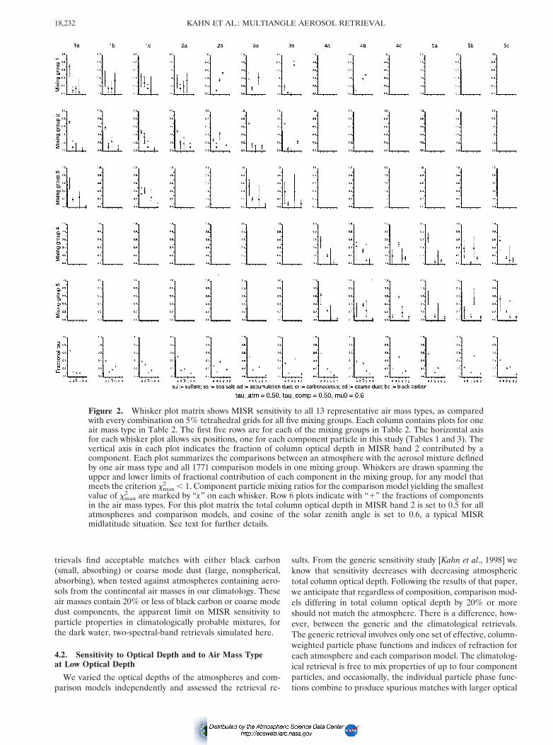
We begin this section by taking a close look at several spe-cific cases and then examine summaries of the entire compar-ison space. Plate 4 shows the results of tests between simulatedMISR measurements for an atmosphere with aerosol air masstype 2a (Table 2) and the 1771 comparison model mixturesthat comprise mixing group 2 (dusty maritime 1 coarse dust).The optical depth in MISR band 2 is set to 0.5 for both theatmosphere and the comparison models in this first example,and typical MISR midlatitude geometry has been adopted; wesubsequently vary the aerosol optical depth systematically overthe entire range from 0.0 to 1.0. The comparison model casesare arranged in a tetrahedron, and Plate 4 shows slices throughthis tetrahedron covering the interesting part of the space.Each pixel is divided into five fields. The upper left subpixel iscolored with the result of the xabs

2 test, the upper right has theresult of the xgeom

2 test, the lower left shows the xmax_dev2 test,

and the lower right contains the xspec2 test, each using the color

bar described in section 3.2. The background is colored withthe result of the most constraining of these four tests (the onewith the highest value), since, if any one of the tests indicatesthat the comparison model does not match the observation, thecomparison model must be rejected. We call this value xmax

2 .Only four planes in Plate 4 have pixels with xmax

2 , 1. So ifwe use this as the criterion for accepting a comparison model,the fraction of the total optical depth contributed by coarsemode dust is constrained to fall between 5% and 20%, since nomodels having coarse mode dust fraction outside this rangematch the observations. Similarly, the sulfate particle mixingratio is confined to the range 50–55%, accumulation modedust must fall between 5 and 35%, and sea salt is constrainedbetween 5 and 25%. Plate 4 also indicates the correlationsamong acceptable fractions for each component. The actualcomposition for air mass type 2a is 10% coarse mode dust,52% sulfate, 21% accumulation mode dust, and 17% sea salt.In this case, the MISR retrieval constrains all the componentparticle types in the mixture to within 15% of their true opticaldepth mixing ratios, and the best constraint is better than 5%.

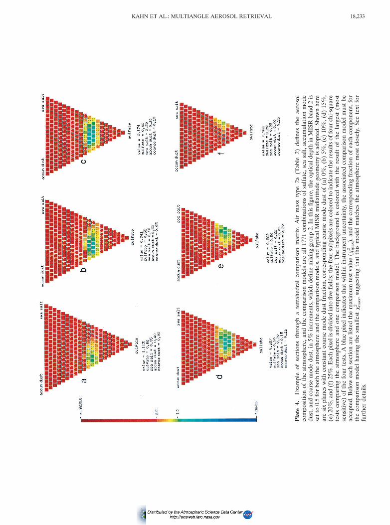
Plates 5a–5d show sections through the tetrahedral compar-ison space for mixing group 4 (carbonaceous 1 dusty conti-nental), for an atmosphere with an aerosol composition givenby air mass type 4a (Table 2). Four planes with constant coarsemode dust mixing ratio, ranging from 0 to 15%, are presented.In this case, the xmax

2 , 1 criterion yields solutions only forcoarse mode dust between 0 and 10% mixing ratio, based onMISR band 2 optical depth contribution, and for accumulationmode dust between 20 and 25%. The sulfate and carbonaceousparticles form a mixing line; models having as much as 70%sulfate (and 0% carbonaceous particles) or as little as 40%sulfate (and 40% carbonaceous particles) meet the acceptancecriterion. For these mixtures of particles over a dark watersurface, a simulated MISR retrieval using the red and near-infrared bands and all nine angles cannot distinguish sulfates,which are “medium, spherical, nonabsorbing” particles, fromcarbonaceous, which are “medium, spherical, absorbing” par-ticles (Table 3). However, the sum of the fractional contribu-tions to optical depth of sulfate and carbonaceous particles isalways around 75%. This is close to the true value, the sum of61% sulfate and 13% carbonaceous particle-mixing ratios.

A similar result appears in Plates 5e–5h, which examines thesensitivity of MISR to an atmosphere having aerosol compo-

sition given by air mass type 4c, in the tetrahedral comparisonspace for mixing group 4. Air mass type 4c contains only 22%sulfate and 11% carbonaceous particle optical depth contribu-tions, along with 51% accumulation mode dust and 16% coarsemode dust. Using the xmax

2 , 1 criterion, acceptable matchesare found for coarse mode dust between 10 and 20%, andaccumulation mode dust from 45 to 55%, reflecting the largerdust contribution for air mass type 4c than for type 4a. Again,sensitivities are around 610% in optical depth mixing ratio,surrounding the expected value, except for sulfate and carbo-naceous aerosols, which form a mixing line.

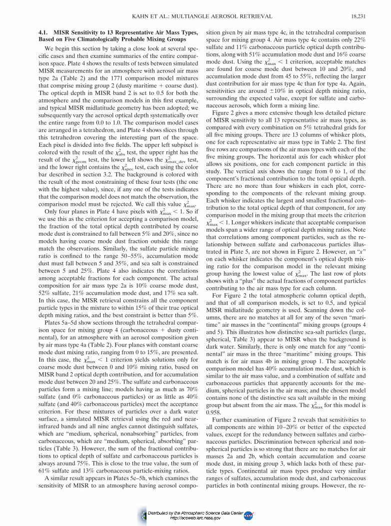
Figure 2 gives a more extensive though less detailed pictureof MISR sensitivity to all 13 representative air mass types, ascompared with every combination on 5% tetrahedral grids forall five mixing groups. There are 13 columns of whisker plots,one for each representative air mass type in Table 2. The firstfive rows are comparisons of the air mass types with each of thefive mixing groups. The horizontal axis for each whisker plotallows six positions, one for each component particle in thisstudy. The vertical axis shows the range from 0 to 1, of thecomponent’s fractional contribution to the total optical depth.There are no more than four whiskers in each plot, corre-sponding to the components of the relevant mixing group.Each whisker indicates the largest and smallest fractional con-tribution to the total optical depth of that component, for anycomparison model in the mixing group that meets the criterionxmax

2 , 1. Longer whiskers indicate that acceptable comparisonmodels span a wider range of optical depth mixing ratios. Notethat correlations among component particles, such as the re-lationship between sulfate and carbonaceous particles illus-trated in Plate 5, are not shown in Figure 2. However, an “x”on each whisker indicates the component’s optical depth mix-ing ratio for the comparison model in the relevant mixinggroup having the lowest value of xmax

2 . The last row of plotsshows with a “plus” the actual fractions of component particlescontributing to the air mass type for each column.

For Figure 2 the total atmospheric column optical depth,and that of all comparison models, is set to 0.5, and typicalMISR midlatitude geometry is used. Scanning down the col-umns, there are no matches at all for any of the seven “mari-time” air masses in the “continental” mixing groups (groups 4and 5). This illustrates how distinctive sea-salt particles (large,spherical, Table 3) appear to MISR when the background isdark water. Similarly, there is only one match for any “conti-nental” air mass in the three “maritime” mixing groups. Thismatch is for air mass 4b in mixing group 1. The acceptablecomparison model has 40% accumulation mode dust, which issimilar to the air mass value, and a combination of sulfate andcarbonaceous particles that apparently accounts for the me-dium, spherical particles in the air mass; and the chosen modelcontains none of the distinctive sea salt available in the mixinggroup but absent from the air mass. The xmax

2 for this model is0.958.

Further examination of Figure 2 reveals that sensitivities toall components are within 10–20% or better of the expectedvalues, except for the redundancy between sulfates and carbo-naceous particles. Discrimination between spherical and non-spherical particles is so strong that there are no matches for airmasses 2a and 2b, which contain accumulation and coarsemode dust, in mixing group 3, which lacks both of these par-ticle types. Continental air mass types produce very similarranges of sulfates, accumulation mode dust, and carbonaceousparticles in both continental mixing groups. However, the re-


trievals find acceptable matches with either black carbon(small, absorbing) or coarse mode dust (large, nonspherical,absorbing), when tested against atmospheres containing aero-sols from the continental air masses in our climatology. Theseair masses contain 20% or less of black carbon or coarse modedust components, the apparent limit on MISR sensitivity toparticle properties in climatologically probable mixtures, forthe dark water, two-spectral-band retrievals simulated here.

4.2. Sensitivity to Optical Depth and to Air Mass Typeat Low Optical Depth

We varied the optical depths of the atmospheres and com-parison models independently and assessed the retrieval re-

sults. From the generic sensitivity study [Kahn et al., 1998] weknow that sensitivity decreases with decreasing atmospherictotal column optical depth. Following the results of that paper,we anticipate that regardless of composition, comparison mod-els differing in total column optical depth by 20% or moreshould not match the atmosphere. There is a difference, how-ever, between the generic and the climatological retrievals.The generic retrieval involves only one set of effective, column-weighted particle phase functions and indices of refraction foreach atmosphere and each comparison model. The climatolog-ical retrieval is free to mix properties of up to four componentparticles, and occasionally, the individual particle phase func-tions combine to produce spurious matches with larger optical

Figure 2. Whisker plot matrix shows MISR sensitivity to all 13 representative air mass types, as comparedwith every combination on 5% tetrahedral grids for all five mixing groups. Each column contains plots for oneair mass type in Table 2. The first five rows are for each of the mixing groups in Table 2. The horizontal axisfor each whisker plot allows six positions, one for each component particle in this study (Tables 1 and 3). Thevertical axis in each plot indicates the fraction of column optical depth in MISR band 2 contributed by acomponent. Each plot summarizes the comparisons between an atmosphere with the aerosol mixture definedby one air mass type and all 1771 comparison models in one mixing group. Whiskers are drawn spanning theupper and lower limits of fractional contribution of each component in the mixing group, for any model thatmeets the criterion xmax

2 , 1. Component particle mixing ratios for the comparison model yielding the smallestvalue of xmax

2 are marked by “x” on each whisker. Row 6 plots indicate with “1” the fractions of componentsin the air mass types. For this plot matrix the total column optical depth in MISR band 2 is set to 0.5 for allatmospheres and comparison models, and cosine of the solar zenith angle is set to 0.6, a typical MISRmidlatitude situation. See text for further details.


Pla

te4.

Exa

mpl

eof

sect

ions

thro

ugh

ate

trah

edra

lco

mpa

riso

nm

atri

x.A

irm

ass

type

2a(T

able

2)de

fines

the

aero

sol

com

posi

tion

ofth

eat

mos

pher

e,an

dth

eco

mpa

riso

nm

odel

sar

eal

l177

1co

mbi

natio

nsof

sulfa

te,s

easa

lt,ac

cum

ulat

ion

mod

edu

st,a

ndco

arse

mod

edu

st,i

n5%

incr

emen

ts,w

hich

defin

em

ixin

ggr

oup

2.In

this

figur

e,th

eop

tical

dept

hin

MIS

Rba

nd2

isse

tto

0.5

for

both

the

atm

osph

ere

and

the

com

pari

son

mod

els,

and

typi

calM

ISR

mid

latit

ude

geom

etry

isad

opte

d.Sh

own

here

are

six

plan

esw

ithco

nsta

ntco

arse

mod

edu

stfr

actio

n,co

rres

pond

ing

coar

sem

ode

dust

of(a

)0%

,(b)

5%,(

c)10

%,(

d)15

%,

(e)

20%

,and

(f)

25%

.Eac

hpi

xeli

sdi

vide

din

tofiv

efie

lds;

the

four

subp

ixel

sar

eco

lore

dto

indi

cate

the

resu

ltsof

four

chi-s

quar

ete

sts

com

pari

ngth

eat

mos

pher

ean

don

eco

mpa

riso

nm

odel

.T

heba

ckgr

ound

isco

lore

dw

ithth

ere

sult

ofth

ela

rges

t(m

ost

sens

itive

)of

the

four

test

s.A

blue

pixe

lind

icat

esth

atw

ithin

inst

rum

ent

unce

rtai

nty,

the

asso

ciat

edco

mpa

riso

nm

odel

mus

tbe

acce

pted

.Bel

owea

chse

ctio

nar

elis

ted

the

max

imum

test

valu

e( x

max

2),

and

the

corr

espo

ndin

gfr

actio

nof

each

com

pone

nt,f

orth

eco

mpa

riso

nm

odel

havi

ngth

esm

alle

stx

max

2,s

ugge

stin

gth

atth

ism

odel

mat

ches

the

atm

osph

ere

mos

tcl

osel

y.Se

ete

xtfo

rfu

rthe

rde

tails

.


Pla

te5.

(a–

d)Sa

me

asPl

ate

4bu

tfo

ran

atm

osph

ere

with

aero

sol

com

posi

tion

give

nby

air

mas

sty

pe4a

(Tab

le2)

and

com

pari

son

mod

els

defin

edby

mix

ing

grou

p4

(car

bona

ceou

s1

dust

yco

ntin

enta

l,T

able

2).S

how

nhe

rear

efo

urpl

anes

havi

ngco

nsta

ntco

arse

mod

edu

stfr

actio

n,co

rres

pond

ing

to(a

)0%

,(b)

5%,(

c)10

%,a

nd(d

)15

%.(

e–h)

Sam

eas

Plat

es5a

–5d

but

with

the

atm

osph

ere

defin

edby

air

mas

sty

pe4c

.The

four

plan

essh

own

are

sect

ions

with

cons

tant

coar

sem

ode

dust

frac

tion,

corr

espo

ndin

gto

(e)

10%

,(f)

15%

,(g)

20%

,and

(h)

25%

.Air

mas

sty

pe4c

cont

ains

39%

less

sulfa

te,3

0%m

ore

accu

mul

atio

nm

ode

dust

,and

11%

mor

eco

arse

mod

edu

stth

anai

rm

ass

type

4a.


depth differences. Fortunately, these tend to be isolated solu-tions, whereas there is usually a range of acceptable modelssurrounding the values for a correct solution, as shown inFigure 2. We further discuss spurious solutions below.

When the 13 atmospheres have optical depth 0.5, there areno matches for comparison models having optical depths lessthan 0.4, for any mixing group. Nor are there any matches forcomparison models with optical depths greater than 0.6, exceptfor several isolated cases. The exceptions involve black carbon,which is in the comparison models but not in the atmospheresfor these cases, and accumulation mode dust, which is in theatmospheres but not the comparison models. Increased blackcarbon fraction substitutes for accumulation mode dust andkeeps the absolute reflectance low, while small adjustments insea salt, sulfate, and carbonaceous fractions complete thematches.

The phase function plots for individual particle types inFigure 1 provide some insight into these spurious cases. Theblack carbon phase function is relatively flat over the range ofscattering angles viewed by the forward cameras (about 608 to1008) and aft cameras (about 1508 to 1608). Since the phasefunction for accumulation mode dust, which is present in theatmospheres but absent from the comparison models, is alsofairly flat over these angles, matches are possible.

Multiple scattering accounts for between 50 and 70% of thesignal in all these cases, so there are limits as to how far it isuseful to carry interpretations based on reasoning from singlescattering. We conclude that we can account qualitatively forthe trends in the spurious matches. If this were a retrievalinvolving real data, such a match would be suspect because (1)only a few isolated cases give matches for each comparisonmodel optical depth, rather than 5% to 20% ranges of frac-tional amounts, as occur for true solutions, and (2) the mixingratio of black carbon, 20% or more, falls significantly outsidethe climatologically probable range.

The situation is far simpler for atmospheres having totalcolumn optical depth 0.5 and comparison models having loweroptical depths. There is no particle in the climatology with arelatively flat scattering phase function that can increase re-flectances, as black carbon lowers them when the comparisonmodel optical depth is higher. For comparison models havingoptical depth below 0.4, there are no matches at all.

When the total atmospheric column aerosol optical depthfalls to between 0.1 and 0.2 in MISR band 2, information aboutparticle properties decreases, the number of matches grows,and some of the substitutions occur more readily than at higheroptical depth. For example, with atmospheric and comparisonmodel optical depths at 0.2, solutions are found in mixinggroup 2 (which is maritime) for all six continental air masstypes, though the amount of sea salt in the solutions is usuallyeither 0 or 5%. In other cases, combinations of accumulationmode dust and carbonaceous particles in a comparison modelcan account for the contributions of coarse mode dust in theatmosphere at these low overall optical depths.

However, even at low optical depths the ability to discrimi-nate large, spherical particles (sea salt), nonspherical particles(accumulation and coarse mode dust), and small, dark parti-cles (black carbon) is preserved, to within 20% of the compo-nent’s true contribution to the total optical depth. In addition,sensitivity to optical depth itself remains high. For an atmo-sphere having 0.2 total column optical depth, there are nomatches at all when the comparison model optical depths are0.15 or lower, or when they are higher than 0.35. As with the

more optically thick atmospheres, spurious matches can occurwhen comparisons are made with models having higher opticaldepth and containing black carbon (mixing groups 3 and 5).Once again, in all these cases, black carbon accounts for aclimatologically high fraction of the total optical depth. Suchcases would be suspect in an actual retrieval.

4.3. Sensitivity Issues Related to Thin Cirrusand to Geographic Latitude

The MISR data processing algorithms use several cloud-detection approaches to eliminate observations containingclouds [e.g., Diner et al., 1998a; Gao and Kaufman, 1995].Although we expect these masks to be effective over a widerange of natural conditions, they are unlikely to be reliablewhen the cirrus normal optical depth is less than a few tenthsat midvisible wavelengths.

Thin cirrus is fundamentally different from the componentparticles considered in previous sections. There are commonmechanisms that form optically thin hazes of cirrus ice crystalsat most latitudes. Climatological constraints on the spatial andtemporal distribution of thin cirrus are so loose that by includ-ing it, we create an additional dimension in the sensitivitystudy.

We performed a preliminary study of four-component mix-tures that include thin cirrus, assuming cirrus microphysicalproperties from the fractal model of Mishchenko et al. [1996],listed in Table 3 and shown in Figure 1. A new set of mixinggroups was created, containing both cirrus and sulfate compo-nents, along with sea salt for maritime groups, accumulationmode dust for the continental groups, and one of the remain-ing entries in Table 1 as the fourth component. New air masstypes were defined, based loosely on the patterns in Table 2,but containing 10, 20, and 50% cirrus contributions to the totalcolumn aerosol optical depth.

The study involved three additional sets of tests: atmo-spheres containing cirrus versus comparison models withoutcirrus, atmospheres without cirrus against comparison modelscontaining cirrus, and atmospheres containing cirrus againstcomparison models containing cirrus. Most of the behaviorfollows patterns described in sections 4.1 and 4.2.

In nearly all cases the retrieval can distinguish thin cirrusfrom other component particles if the total column aerosoloptical depth is greater than about 0.2 and the cirrus contri-bution is more than about 20%. The ability of MISR to identifyaerosol air mass types is significantly reduced when cirrus ispresent, but the sensitivity to total aerosol optical depth is notdiminished. A more extensive study of thin cirrus sensitivity,one that incorporates several cirrus particle models as well ascomparisons with MISR observations, will be the subject of afuture paper.

Since the range of scattering angles observed by MISR var-ies with latitude, we also expanded the sensitivity study toinclude high- and low-latitude cases. At high latitudes therange of scattering angles sampled by MISR increases, extend-ing from about 408 to 1608. The patterns are very similar tothose at midlatitudes; the lengths of whiskers are shorter insome cases but not significantly so relative to the ranges ofuncertainty. At low latitudes, scattering angle coverage is lim-ited to between about 1058 and 1658. Whisker lengths arelonger in some cases, and a few more coincidental matchesoccur, but the conclusions of this and previous sections remainintact.


5. Discussion and ConclusionsIn earlier theoretical work we performed generic retrieval

simulations for a MISR-like instrument. Such retrievals makea minimum of assumptions about the particles present andseek column-averaged, cross-section-weighted mean aerosolproperties. The results provide insight into the informationcontent of the observations. We found that for natural rangesof particle properties, under good observing conditions, theMISR retrieval can make about a dozen distinctions based onparticle size (small, medium, large), shape (spherical and ran-domly oriented nonspherical), and composition (absorbing andnonabsorbing), along with estimates of aerosol column opticaldepth.

A limitation of the generic retrieval approach is that cross-section-weighted mean aerosol properties are difficult to com-pare with in situ and field measurements, and with the resultsof any physically based aerosol transport model, since thesedescribe the behavior of mixtures of component particles. Thecurrent paper explores climatological retrievals for simulatedMISR data. Such retrievals constrain the proportions of indi-vidual components in climatologically probable mixtures. Weconclude that multiangle, multispectral imaging containsenough information about particle properties to warrantadopting this retrieval approach as well.

Since the value of a climatological retrieval depends on thequality of an assumed climatology, we base our assumptions onresults from some of the best available global, monthly aerosoltransport models. Our analysis shows that the entire global,monthly data set, aggregated from transport models for the sixmost common component particles, can be represented by aclimatology containing only five mixing groups, each composedof all possible proportions of four externally mixed compo-nents. The mixing groups define the climatological retrievalcomparison space. We also find that within each mixing group,the climatologically probable mixtures cluster into only two orthree representative air mass types, having specific proportionsof the four components in that group. For the sensitivity study,these representative air mass types characterize the sampleatmospheres that are tested against the comparison space. Themixing group and representative air mass type results are sum-marized in Table 2 and Plate 1.

To complete the climatology, we must assume microphysicalproperties for each component aerosol (Table 3). The valuesused here were obtained from standard sources and reflect thecharacteristic differences among component particles. How-ever, detailed microphysical properties of component particlesvary with source region and air mass meteorological history.When performing retrievals with MISR data, we anticipateusing additional constraints from in situ and field measure-ments whenever possible to reduce the uncertainties.

On the basis of midlatitude simulations, for the assumedclimatology, good viewing conditions, and moderate aerosoloptical depth (nominally 0.5 at 0.56 mm wavelength), MISRcan retrieve sea salt (large, spherical particles) and accumula-tion mode dust (medium, nonspherical particles) to within20% of the true mixing ratio or better. This is sufficient todistinguish maritime from continental aerosol air masses.MISR retrievals over dark water, using nine angles and the redand near-IR channels, are not good at distinguishing sulfates(medium, spherical, nonabsorbing) from carbonaceous parti-cles (medium, spherical, absorbing); however, the sum is re-trieved to within 20% of the true mixing ratio or better.

Coarse mode dust and black carbon particles contribute lessthan 20% to the total column aerosol optical depth everywherein the climatology. Though models having the correct compo-sition usually yield the lowest xmax

2 , comparison models withadjusted amounts of other components can usually be found tomeet the acceptance criterion for atmospheres containing theless abundant particles.

In spite of the added flexibility offered by the climatologicalretrieval in allowing mixtures of components having differentsingle-scattering phase functions, constraints on total aerosoloptical depth are nearly as tight as those for the generic re-trieval. With an atmospheric aerosol optical depth of 0.5 nocomparison models having optical depth less than 0.4 orgreater than 0.75 match any of the atmospheres. The matchingcomparison models having optical depths greater than 0.60 allcontain large fractions of black carbon, and most are isolatedsolutions that arise from fortuitous combinations of particle-scattering phase functions. In actual retrievals, such caseswould be suspect, because (1) retrieved component mixingratios for true solutions are not isolated; they typically span arange of 5–20%, and (2) mixtures containing 20% or moreblack carbon are climatologically improbable.

When the total atmospheric aerosol column optical depth isreduced to 0.2, the constraints are looser than for the 0.5 cases,and some substitutions of component particles occur morereadily. However, the ability to distinguish large, spherical par-ticles (sea salt), nonspherical particles (accumulation andcoarse mode dust), and small, dark particles (black carbon) ispreserved, at least to within 20% or better of the expectedvalues; and even with reduced sensitivity to particle microphys-ical properties, the total aerosol optical depth is constrained to0.05 or better, if one rejects cases having implausibly largefractions of black carbon or coarse mode dust.

We can relate the climatological retrieval approach devel-oped here to other satellite aerosol retrievals. The MISR cli-matological retrieval looks at five mixing groups, each com-posed of four component particles in all possible combinations.Each mixing group can be represented by a tetrahedron, asdescribed in sections 2.1 and 4.1.

The AVHRR phases 1 and 2 aerosol retrieval algorithms[Stowe et al., 1997] can be viewed as climatological retrievalsthat interpret one-channel measurements using one vertex ofone tetrahedron as the comparison space. For the phase 2algorithm, a medium spherical (sulfate-like) particle type isassumed, having a lognormal size distribution with character-istic radius 0.1 mm, width 2.03, and index of refraction 1.4 20.0i. For interpreting single-channel observations the aerosolclimatology developed for the MISR analysis seems to supportthis choice; sulfates are the only particles common to all airmass types, and they frequently account for a substantial frac-tion of the column aerosol optical depth, particularly overocean.

Many two-channel AVHRR algorithms are cast as genericrather than climatological retrievals [e.g., Durkee et al., 1991;Stowe et al., 1997; Mishchenko et al., 1999]. These produceaerosol column optical depth, and a constraint on columnmean, cross-section-weighted particle size from a continuum ofpossible values, for assumed particle size distribution function,particle shape, and indices of refraction; but here the linebetween generic and climatological retrievals blurs. Havingassumed size distribution function, shape, and indices of re-fraction, the ratio of two-component particles can be uniquelycalculated from a retrieved size constraint such as a value of


the Angstrom coefficient. Attempts are made in these studiesto interpret the size constraints resulting from the retrievals interms of climatologically probable components.

A retrieval developed for AVHRR [Higurashi and Naka-jima, 1998], and also applied to the OCTS instrument [Naka-jima and Higurashi, 1998; Nakajima et al., 1999], takes a clima-tological approach, solving explicitly for the ratio of small tolarge particle components along with aerosol column opticaldepth. This retrieval assumes two lognormal distributions ofspherical particles having characteristic radii 0.17 and 3.44 mm,and for the OCTS case, widths 1.3 and 2.75, respectively. Theindex of refraction is set to 1.5 2 0.005i for all particles. Thisapproach amounts to using the edge of one tetrahedron as thecomparison space. The components chosen are a mediumspherical particle (corresponding to the carbonaceous or sul-fate components in the MISR climatology) and a large spher-ical particle (similar to the MISR sea salt, though larger). Theresults of the present study seem to fit well with this selection.Of the six components in the MISR retrieval, sulfate andcarbonaceous particles are difficult for satellite remote sensinginstruments to distinguish over dark water. Spherical and non-spherical particles are difficult to distinguish for instrumentslacking multiangle capability, and sensitivity to small, darkparticles (black carbon) over dark water is not so high as forother components. This collapses the MISR six-componentcomparison space down to one large spherical and one me-dium spherical component.

The standard dark water aerosol retrieval for the multispec-tral, nadir-looking Moderate-Resolution Imaging Spectroradi-ometer (MODIS) instrument, flying on the Terra platformalong with MISR, is a hybrid of generic and climatologicalapproaches [Tanre et al., 1997]. The algorithm solves for aero-sol column optical depth and the ratio of contributions frompairs of lognormally distributed components, one mediumspherical, the other, large spherical. However, in addition, theretrieval selects a best fit medium spherical component fromamong five options having incrementally different radii, widths,and indices of refraction. Similarly, the large spherical compo-nent is selected from among six options.

From an aerosol climatology perspective, one qualitativelynew contribution of MISR is an ability to distinguish sphericalfrom nonspherical particles. We are driven to create a com-parison space of five four-component mixing groups so we canexplicitly include climatologically important coarse dust andblack carbon components, to which MISR has some sensitivity,but which are rarely among the two or three most abundantparticles in natural air masses. By reporting the range of ac-ceptable solutions over an extensive, climatologically basedcomparison space, the MISR climatological retrieval distin-guishes among aerosol air mass types with passive remotesensing observations.

In this series of MISR aerosol retrieval papers, we havesorted through an enormous amount of simulated data. Wehave identified patterns in the MISR sensitivity to atmosphericaerosols using both a column-average-particle “generic” ap-proach and a retrieval strategy for aerosol mixtures whichrelies on a climatology of component particles having assumedmicrophysical properties. The retrievals were performed usingthe MISR red and near-infrared channels, at all nine lookangles, over dark water. Enhancements to these retrieval strat-egies are possible, such as including data from the MISR blueor green channels, if issues of ocean surface reflectance atthese wavelengths and increased sensitivity to the vertical dis-

tribution of aerosols can be addressed. We may find ways toimprove aerosol retrieval sensitivity by incorporating data fromother instruments, such as longer wavelength channels fromMODIS.

However, it is time to look at real data. With instrumentobservations, uncertainties introduced by specific attributes ofthe environment will need to be considered: the vertical dis-tribution of aerosols, the surface bidirectional reflectance func-tion, the actual physical properties of the aerosols and anycirrus ice crystals present, and variability of surface and aerosolproperties within the scene. Where possible, we will rely on insitu and field measurements to help constrain the solutionspace. Analysis of observations from AirMISR, the aircraftversion of our multiangle instrument [Diner et al., 1998b], is thesubject of continuing work [Kahn et al., 2000]; and we are justbeginning to look at data from MISR itself.

Acknowledgments. We thank Jeff Kiehl, Joyce Penner, LarryStowe, and Ina Tegen for sharing their aerosol data with us, SundarChristopher, Yoram Kaufman, Michael Mishchenko, Lorraine Remer,and Irina Sokolik for valuable discussions about particle properties,and Amy Braverman, David Diner, and John Martonchik for discus-sions on a wide range of related scientific issues. This research issupported by the EOS-MISR instrument program, and by the Climateand Radiation Research and Analysis Program in the Earth SciencesDivision of the National Aeronautics and Space Administration, underR. Curran. This work is performed at the Jet Propulsion Laboratory,California Institute of Technology, under contract with NASA.

ReferencesAbdou, W. A., J. V. Martonchik, R. Kahn, R. West, and D. Diner, A

modified linear-mixing method for calculating atmospheric path ra-diances of aerosol mixtures, J. Geophys. Res., 102, 16,883–16,888,1997.

Andreae, M. O., Climatic effects of changing atmospheric aerosollevels, in World Survey of Climatology, vol. 16, Future Climates of theWorld, A. Henderson-Sellers (Ed.), pp. 341–392, Elsevier Sci., NewYork, 1995.

Bevington, P. R., and D. K. Robinson, Data Reduction and ErrorAnalysis for the Physical Sciences, 2nd ed., 328 pp., McGraw-Hill,New York, 1992.

Bruegge, C. J., V. G. Duval, N. L. Chrien, R. P. Korechoff, B. J.Gaitley, and E. B. Hochberg, MISR prelaunch instrument calibra-tion and characterization results, IEEE Trans. Geosci. Remote Sens.,36, 1186–1198, 1998.

Charlson, R. J., S. Schwartz, J. Hales, R. Cess, J. Coakley Jr.,J. Hansen, and D. Hofmann, Climate forcing by anthropogenicaerosols, Science, 255, 423–430, 1992.

Chin, M., D. J. Jacob, G. M. Gardner, P. A. Spiro, M. Foreman-Fowler, and D. L. Savoie, A global three-dimensional model oftropospheric sulfate, J. Geophys. Res., 101, 18,669–18,690, 1996.

Cusack, S., A. Slingo, J. M. Edwards, and M. Wild, The radiativeimpact of a simple aerosol climatology on the Hadley Centre atmo-spheric GCM, Q. J. R. Meteorol. Soc., 124, 2517–2526, 1998.

d’Almeida, G. A., P. Koepke, and E. P. Shettle, Atmospheric Aerosols:Global Climatology and Radiative Characteristics, A. Deepak, Hamp-ton, Va., 1991.

Deschamps, P. Y., F. M. Breon, M. Leroy, A. Podaire, A. Brichaud,J. C. Buriez, and G. Seze, The POLDER mission: Instrument char-acteristics and scientific objectives, IEEE Trans. Geosci. RemoteSens., 32, 598–615, 1994.

Diner, D. J., et al., Multiangle Imaging SpectroRadiometer (MISR)description and experiment overview, IEEE Trans. Geosci. RemoteSens., 36, 1072–1087, 1998a.

Diner, D. J., et al., The Airborne Multi-angle Imaging SpectroRadi-ometer (AirMISR): Instrument description and first results, IEEETransact. Geosci. Remote Sens., 36, 1339–1349, 1998b.

Durkee, P. A., F. Pfeil, E. Frost, and R. Shema, Global analysis ofaerosol particle characteristics, Atmos. Environ., Ser. A, 25, 2457–2471, 1991.


Gao, B.-C., and Y. J. Kaufman, Selection of the 1.375-mm MODISchannel for remote sensing of cirrus clouds and stratospheric aero-sols from space, J. Atmos. Sci., 52, 4231–4237, 1995.

Grant, I. P., and G. E. Hunt, Solution of radiative transfer problemsusing invariant Sn method, Mon. Not. R. Astron. Soc., 141, 27–41,1968.

Hanel, G., The properties of atmospheric aerosol particles as functionsof relative humidity at thermodynamic equilibrium with the sur-rounding moist air, Adv. Geophys., 19, 73–188, 1976.

Hansen, J. E., and L. D. Travis, Light scattering in planetary atmo-spheres, Space Sci. Rev., 16, 527–610, 1974.

Hansen, J., M. Sato, A. Lacis, and R. Ruedy, The missing climateforcing, Philos. Trans. R. Soc. London, Ser. B, 352, 231–240, 1997.

Hartigan, J. A., and M. A. Wong, Algorithm AS 136: A K-meansclustering algorithm, Appl. Stat., 28, 100–108, 1979.

Haywood, J. M., V. Ramaswamy, and B. J. Soden, Tropospheric aero-sol climate forcing in clear-sky satellite observations over the oceans,Science, 283, 1299–1303, 1999.

Hegg, D., T. Larson, and P.-F. Yuen, A theoretical study of the effectof relative humidity on light scattering by tropospheric aerosols, J.Geophys. Res., 98, 18,435–18,439, 1993.

Herman, J. R., P. K. Bhartia, O. Torres, C. Hsu, C. Seftor, andE. Celarier, Global distribution of UV-absorbing aerosols fromNimbus 7/TOMS data, J. Geophys. Res., 102, 16,911–16,922, 1997.

Higurashi, A., and T. Nakajima, Development of a two-channel aero-sol retrieval alogrithm on a global scale using NOAA AVHRR, J.Atmos. Sci., 56, 924–941, 1999.

Husar, R. B., J. M. Prospero, and L. L. Stowe, Characterization oftropospheric aerosols over ocean with the NOAA-advanced veryhigh resolution radiometer optical thickness operational product, J.Geophys. Res., 102, 16,889–16,909, 1997.

Kahn, R., R. West, D. McDonald, B. Rheingans, and M. I. Mish-chenko, Sensitivity of multiangle remote sensing observations toaerosol sphericity, J. Geophys. Res., 102, 16,861–16,870, 1997.

Kahn, R., P. Banerjee, D. McDonald, and D. Diner, Sensitivity ofmultiangle imaging to aerosol optical depth, and to pure-particlesize distribution and composition over ocean, J. Geophys. Res., 103,32,195–32,213, 1998.

Kahn, R., P. Banerjee, D. McDonald, and J. V. Martouchik, Aerosolproperties derived from aircraft multiangle imaging over MontereyBay, J. Geophys. Res., in press, 2000.

Kopke, P., M. Hess, I. Schult, and E. Shettle, Global aerosol data set,Max Planck Inst. Meterol. Rep., 243, Hamburg, Germany, 1997.

Li, Z., L. Moreau, and A. Arking, On solar energy disposition: Aperspective from observation and modeling, Bull. Am. Meteorol.Soc., 78, 53–70, 1997.

Liousse, C., J. Penner, C. Chuang, J. Walton, H. Eddleman, andH. Cachier, A global three-dimensional model study of carbona-ceous aerosols, J. Geophys. Res., 101, 19,411–19,432, 1996.

Martonchik, J. V., D. J. Diner, R. Kahn, M. M. Verstraete, B. Pinty,H. R. Gordon, and T. P. Ackerman, Techniques for the retrieval ofaerosol properties over land and ocean using multiangle imaging,IEEE Trans. Geosci. Remote Sens., 36, 1212–1227, 1998.

Mishchenko, M. I., W. B. Rossow, A. Macke, and A. A. Lacis, Sensi-tivity of cirrus cloud albedo, bidirectional reflectance and opticalthickness retrieval accuracy to ice particle shape, J. Geophys. Res.,101, 16,973–16,985, 1996.

Mishchenko, M. I., L. Travis, R. Kahn, and R. West, Modeling phasefunctions for dust-like tropospheric aerosols using a shape mixture

of randomly oriented polydisperse spheroids, J. Geophys. Res., 102,16,831–16,847, 1997.

Mishchenko, M. I., I. V. Geogdzhayev, B. Cairns, W. B. Rossow, andA. Lacis, Aerosol retrievals over the ocean by use of channels 1 and2 AVHRR data: Sensitivity analysis and preliminary results, Appl.Opt., 38, 7325–7341, 1999.

Nakajima, T., and A. Higurashi, A use of two-channel radiances for anaerosol characterization from space, Geophys. Res. Lett., 25, 3815–3818, 1998.

Nakajima, T., A. Kigurashi, K. Aoki, T. Endoh, H. Fukushima,M. Toratani, Y. Mitomi, B. G. Mitechell, and R. Frouin, Earthphase analysis of OCTS radiance data for aerosol remote sensing,IEEE Trans. Geosci. Remote Sens., 37, 1575–1585, 1999.

Penner, J. E., R. J. Charlson, J. M. Hales, N. S. Laulainen, R. Leifer,T. Novakov, J. Ogren, L. F. Radke, S. E. Schwartz, and L. Travis,Quantifying and minimizing uncertainty of climate forcing by an-thropogenic aerosols, Bull. Am. Meteorol. Soc., 75, 375–400, 1994.

Prospero, J. M., R. J. Charlson, V. Mohnen, R. Jaenicke, A. C. Delany,J. Moyers, W. Zoller, and K. Rahn, The atmospheric aerosol system:An overview, Rev. Geophys. Space Phys., 21, 1607–1629, 1983.

Rao, C. R. N., L. L. Stowe, and E. P. McClain, Remote sensing ofaerosols over the oceans using AVHRR data: Theory, practice andapplications, Int. J. Remote Sens., 10, 743–749, 1989.

Reid, J. S., P. V. Hobbs, R. J. Ferek, D. R. Blake, J. V. Martins, M. R.Dunlap, and C. Liousse, Physical, chemical, and optical properties ofregional hazes dominated by smoke in Brazil, J. Geophys. Res., 103,32,059–32,080, 1998.

Shettle, E. P., and R. W. Fenn, Models for the aerosols of the loweratmosphere and the effects of humidity variations on their opticalproperties, AFGL-TR-79-0214, 94 pp., Air Force Geophys. Lab.,Bedford, Mass., 1979.

Sokolik, I. N., and O. B. Toon, Direct radiative forcing by anthropo-genic airborne mineral aerosols, Nature, 381, 681–683, 1996.

Stowe, L. L., A. M. Ignatov, and R. R. Singh, Development, validation,and potential enchancements to the second-generation operationalaerosol product at the National Environmental Satellite, Data, andInformation Service of the National Oceanic and Atmospheric Ad-ministration, J. Geophys. Res., 102, 16,923–16,934, 1997.

Tanre, D., Y. J. Kaufman, M. Herman, and S. Mattoo, Remote sensingof aerosols over oceans using the MODIS/EOS spectral radiances, J.Geophys. Res., 102, 16,971–16,988, 1997.

Tegen, I., and I. Fung, Contribution to the atmospheric mineral aero-sol load from land surface modification, J. Geophys. Res., 100,18,707–18,726, 1995.

Tegen, I., P. Hollrig, M. Chin, I. Fung, D. Jacob, and J. Penner,Contribution of different aerosol species to the global aerosol ex-tinction optical thickness: Estimates from model results, J. Geophys.Res., 102, 23,895–23,915, 1997.

World Climate Programme (WCP), A preliminary cloudless standardatmosphere for radiation computation, WCP-112, 53 pp., Int. Assoc.for Meteorol. and Atmos. Phys., Boulder, CO, 1984.

P. Banerjee, R. Kahn, and D. McDonald, Jet Propulsion Laboratory,California Institute of Technology, MS 169-237, 4800 Oak GroveDrive, Pasadena CA 91109. ([email protected])

(Received November 30, 1999; revised July 24, 2000;accepted July 31, 2000.)


Documents

Sensitivity of multiangle imaging to natural mixtures … of multiangle imaging to natural mixtures of aerosols over ocean Ralph Kahn, Pranab Banerjee, and Duncan McDonald Jet Propulsion