Sensitivity of fluid flow to fault core architecture and petrophysicalproperties of fault rocks in siliciclastic reservoirs: a synthetic fault

model study

Niclas Fredman1,2, Jan Tveranger1, Siv Semshaug1, Alvar Braathen1,3 and Einar Sverdrup4

1Centre for Integrated Petroleum Research, University of Bergen, Allégaten 41, N-5007 Bergen, Norway2Present address: Statoil ASA, Strandveien 4, N-7500 Trondheim, Norway (e-mail: NICF@statoil.com)

3Present address: University Centre in Svalbard, 9171 Longyearbyen, Norway4Ener Petroleum ASA, PO Box 128, N-1325 Lysaker, Norway

ABSTRACT: Fluid flow simulation models of faulted reservoirs normally includefaults as grid offset in combination with 2D transmissibility multipliers. Thisapproach tends to oversimplify the way effects caused by the actual 3D architectureof fault zones are handled. By representing faults as 3D rock volumes in reservoirmodels, presently overlooked structural features may be included and potentiallyyield a more realistic description of structural heterogeneities. This paper describes afirst effort to map the effect, including a volumetric fault zone description, has onfluid flow simulation.

An experimental 3D model grid including a single normal fault, defined as avolumetric grid, was constructed. Subsequently, the fault grid was populated withtwo conceptual fault deformation products – sand lenses and fault rock – using anobject-based stochastic facies modelling technique. In order to evaluate the effect ofvarying petrophysical properties, fault rock permeability and sand lens permeabilitywere varied deterministically between 0.01 mD and 1 mD and 50 mD and 500 mD,respectively. The impact of fault core architecture was investigated by deterministi-cally varying sand lens fraction and sand lens connectivity. This yielded 24 modelconfigurations, executed in 20 stochastic realizations each. Fluid flow simulation wasperformed on 480 model realizations.

Simulation results show that the most important parameters influencing fluid flowacross the fault were fault rock matrix permeability, and whether or not the sandlenses were connected to the undeformed host rock. Sand lens permeability and sandlens fraction turned out to be less important for fluid flow than fault rock matrixpermeability and sand lens connectivity.

KEYWORDS: fault modelling, fluid flow, fault facies, stochastic modelling

INTRODUCTION

Reservoir uncertainty characterization and fluid flow simulationare important tools when trying to understand and predictreservoir performance. To date, most efforts have focused onestablishing uncertainties attached to sedimentological par-ameters. Studies focusing on structural parameters, in contrast,have been fewer, and a reservoir model is often restricted to asingle or a few deterministic, structural models (Lescoffit &Townsend 2002; Ottesen et al. 2005). Considering the impactfaults have on reservoir fluid flow (Bouvier et al. 1989; Knipe1992; Gibson 1998; Manzocchi et al. 1999; Fisher et al. 2001;Fisher & Knipe 2001; Shipton et al. 2002), further studies aimedat quantifying how structural factors affect reservoir perform-ance are clearly needed. Furthermore, these studies should notbe limited by restrictions imposed by the currently availablemodelling tools, but use field observations as their startingpoint. Several workers have investigated the impact of sub-seismic faulting, fault geometry, fault density, fault displace-

ment and sealing properties (e.g. Damsleth et al. 1998; England& Townsend 1998; Hollund et al. 2002; Lescoffit & Townsend2002; Holden et al. 2003; Ottesen et al. 2005; Tveranger et al.2007). Previous studies have also used discrete grid cells toinvestigate single- (López & Smith 1996; Caine & Forster 1999;Flodin et al. 2001) and multi-phase flow properties of faultrocks (e.g. Manzocchi et al. 1998, 2002; Rivenæs & Dart 2002;Al Busafi et al. 2005). Volumetric fault modelling of fault corearchitecture, in contrast, is still novel work and few publicationsare available. Berg & Øian (2007) used a hierarchical, determin-istic model to investigate the effect of fault zone architecture onmulti-phase flow. Nøttveit (2005) also used a hierarchicalapproach for volumetric modelling of fault zone architectureand fractures.

Field studies suggest that fault zones can be divided into twomain elements (Fig. 1); the central fault core and the outer,surrounding damage zone (e.g. Caine et al. 1996). In poorlylithified sediments this subdivision can be extended by adding a

Petroleum Geoscience, Vol. 13 2007, pp. 1–16 1354-0793/07/$15.00 � 2007 EAGE/Geological Society of London

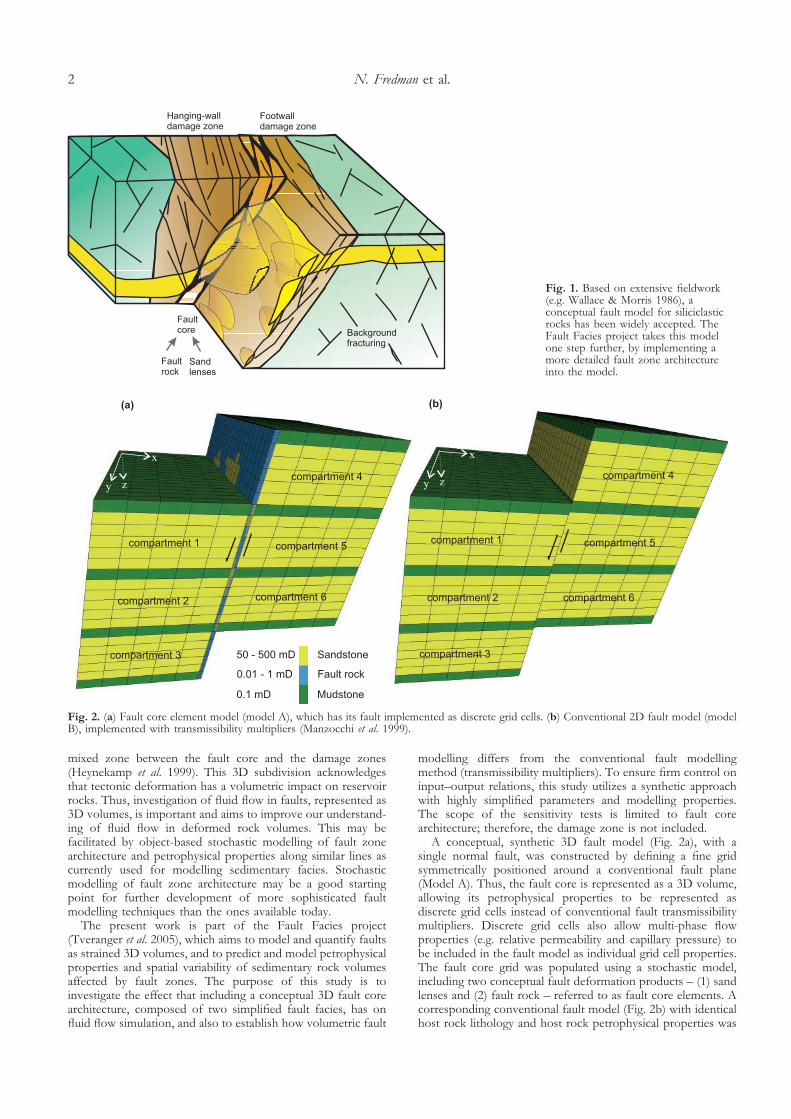
mixed zone between the fault core and the damage zones(Heynekamp et al. 1999). This 3D subdivision acknowledgesthat tectonic deformation has a volumetric impact on reservoirrocks. Thus, investigation of fluid flow in faults, represented as3D volumes, is important and aims to improve our understand-ing of fluid flow in deformed rock volumes. This may befacilitated by object-based stochastic modelling of fault zonearchitecture and petrophysical properties along similar lines ascurrently used for modelling sedimentary facies. Stochasticmodelling of fault zone architecture may be a good startingpoint for further development of more sophisticated faultmodelling techniques than the ones available today.

The present work is part of the Fault Facies project(Tveranger et al. 2005), which aims to model and quantify faultsas strained 3D volumes, and to predict and model petrophysicalproperties and spatial variability of sedimentary rock volumesaffected by fault zones. The purpose of this study is toinvestigate the effect that including a conceptual 3D fault corearchitecture, composed of two simplified fault facies, has onfluid flow simulation, and also to establish how volumetric fault

modelling differs from the conventional fault modellingmethod (transmissibility multipliers). To ensure firm control oninput–output relations, this study utilizes a synthetic approachwith highly simplified parameters and modelling properties.The scope of the sensitivity tests is limited to fault corearchitecture; therefore, the damage zone is not included.

A conceptual, synthetic 3D fault model (Fig. 2a), with asingle normal fault, was constructed by defining a fine gridsymmetrically positioned around a conventional fault plane(Model A). Thus, the fault core is represented as a 3D volume,allowing its petrophysical properties to be represented asdiscrete grid cells instead of conventional fault transmissibilitymultipliers. Discrete grid cells also allow multi-phase flowproperties (e.g. relative permeability and capillary pressure) tobe included in the fault model as individual grid cell properties.The fault core grid was populated using a stochastic model,including two conceptual fault deformation products – (1) sandlenses and (2) fault rock – referred to as fault core elements. Acorresponding conventional fault model (Fig. 2b) with identicalhost rock lithology and host rock petrophysical properties was

Fig. 1. Based on extensive fieldwork(e.g. Wallace & Morris 1986), aconceptual fault model for siliciclasticrocks has been widely accepted. TheFault Facies project takes this modelone step further, by implementing amore detailed fault zone architectureinto the model.

Fig. 2. (a) Fault core element model (model A), which has its fault implemented as discrete grid cells. (b) Conventional 2D fault model (modelB), implemented with transmissibility multipliers (Manzocchi et al. 1999).

N. Fredman et al.2

also constructed using 2D fault transmissibility multipliers(model B). Fluid flow simulation was executed and set up as atwo-phase flow using oil and water.

FAULTS IN RESERVOIR MODELLING

Faults in flow simulation

It is generally accepted that faults can act as both barriers andconduits to fluid flow (Antonellini & Aydin 1994; Caine et al.1996; Fulljames & Zalán 1997; Fisher & Knipe 1998, 2001).There are two processes that can form a sealing fault: (1)juxtaposing a unit with zero permeability against a reservoirunit; or (2) sealing fault rock development, i.e. membrane seal(e.g. Fisher & Knipe 1998; Sperrevik et al. 2002; Yielding 2002).Cementation seals may also develop (Fisher et al. 2000), butthese are not considered here.

A number of software packages allow users to build sophis-ticated 3D geological models that serve as input to fluidflow simulators (e.g. IRAP-RMSTM, PetrelTM, GocadTM). Theconventional way of including faults in these models is toimplement cross-fault flow properties as fault transmissibilitymultipliers (Manzocchi et al. 1999). What these software solu-tions have in common is that they describe fault permeabilityand transmissibility as 2D properties attached to a fault plane.Consequently, 3D fault core architecture is largely ignored andfeatures, such as intra-fault vertical fluid flow, can be handledonly ad hoc, using deterministic methods.

A common approach to calculate fault transmissibility mul-tipliers is to use the Shale Gouge Ratio (SGR) algorithm (1),defined by Yielding et al. (1997) and the fault zone permeabilityalgorithm (2), defined by Manzocchi et al. (1999).

SGR = �shale_bed_thicknessfault_throw

(1)

log �kfz� = � 4SGR �14

log �D��1 � SGR�5 (2)

In equation (1), shale_bed_thickness is the total amount ofimpure material that has slipped past a particular point on thefault, and fault_throw is the total fault throw. In equation (2),SGR is the Shale Gouge Ratio, D is the fault displacement (m)and kfz is the fault zone permeability (mD). Fault zonedisplacement/thickness relationships (Hull 1988; Evans 1990;Knott et al. 1996; Foxford et al. 1998; Walsh et al. 1998;Sperrevik et al. 2002), Clay Smear Potential (Bouvier et al. 1989)and Shale Smear Factor (Lindsay et al. 1993) are also commonconstituents in fault transmissibility multiplier calculations.Stand-alone SGR curves can also be used, allowing users todefine their own SGR/fault zone permeability relationship.

Typically, the shale content is described by a Vshale parameterin a standard reservoir model. It is also possible to includeeffects of brittle deformation, cementation and effects related tomaximum burial depth and depth at time of deformation.Another important – and expedient – technique in fault sealanalysis is to use juxtaposition and fault seal diagrams (Childs etal. 1997; Knipe 1997) to evaluate the sealing capacity. Formature fields, or at least for those fields for which someproduction data are available, fault transmissibility multiplierscan also be derived deterministically from history matching.This may result in transmissibility multipliers with limitedrelation to the actual structural geology. Deterministic historymatching based on homogeneous transmissibility multipliers isable to match present-day history, but may have poor predictivevalue (Ottesen et al. 2005).

Fault core architecture and permeability structure

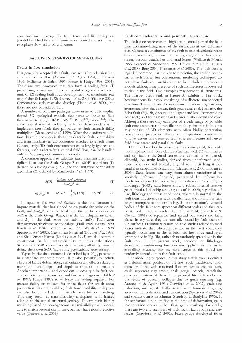
The fault core represents the high-strain central part of the faultzone accommodating most of the displacement and deforma-tion. Common constituents of the fault core in siliciclastic rocksof extensional regimes include: fault gouge, slip surfaces, claysmear, breccia, cataclasites and sand lenses (Wallace & Morris1986; Peacock & Sanderson 1992; Childs et al. 1996; Clausenet al. 2003; Berg 2004; Kristensen et al. 2005). The fault core isregarded commonly as the key to predicting the sealing poten-tial of fault zones, but conventional modelling techniques donot allow fault core architecture to be included in reservoirmodels, although the presence of such architectures is observedreadily in the field. Two examples may serve to illustrate this.The Hartley Steps fault in Figure 3a exhibits a 1 m thick,heterogeneous fault core consisting of a discrete, unconnectedsand lens. The sand lens shows downwards-increasing rotation,intermixed with shale smear, fault gouge and coal. Similarly, theBaba fault (Fig. 3b) displays one larger sand lens (connected tohost rock) and four smaller sand lenses further down the core.Although these are only examples of a wide range of possiblefault core architectures, they illustrate the point that fault coresmay consist of 3D elements with often highly contrastingpetrophysical properties. The important question to answer isto what extent this observed fault core architecture influencesfluid flow across and parallel to faults.

The model used in the present study is conceptual, thus, onlytwo simplified fault core elements are included: (1) sand lensesand (2) fault rock. Sand lenses are defined as elongated,ellipsoid, low-strain bodies, derived from undeformed sand-stone host rock and typically aligned with their longest axisparallel or subparallel to fault dip (Clausen et al. 2003; Lindanger2003). Sand lenses can vary from almost undeformed tointensely deformed, fractured, penetrated by deformationbands and exposed for secondary mineralization. According toLindanger (2003), sand lenses show a robust internal relativegeometrical relationship (x-: y-: z-axis of 1: 10: 9), regardless ofsize, lithology and stress conditions, where x is normal to thefault (lens thickness), y is fault parallel (lens width) and z is lensheight (compare to the lens in Fig. 3 for orientation). Lensoidbodies of the fault core appear on different scales and they canbe stacked on top of each other (Gibbs 1984; Gabrielsen &Clausen 2001) or separated and spread out across the faultplane. In any case, they are normally bound by fault rocks orslip surfaces. Preliminary results on field studies related to sandlenses indicate that when represented in the fault core, theytypically occur near to the undeformed host rock sand layer(exemplified in Fig. 3b), rather than randomly spread out in thefault core. In the present work, however, no lithology-dependent conditioning function was applied for the faciesmodelling, meaning that the sand lenses in this model arerandomly spread out in the fault core.

For modelling purposes, in this study a fault rock is definedas a deformation product of the host rock (mudstone, sand-stone or both), with modified flow properties and, as such,could represent clay smear, shale gouge, breccia, cataclasiteor a combination of these. Low permeability fault rocks arethe result of porosity collapse due to grain crushing (e.g.Antonellini & Aydin 1994; Crawford et al. 2002), grain-sizereduction, mixing of phyllosilicates with framework grains,increased mineralization and cementation (Sperrevik et al. 2002)and contact quartz dissolution (Sverdrup & Bjørlykke 1996). Ifthe sandstone is non-lithified at the time of deformation, grainre-orientation occurs rather than grain crushing. Generally,there are two end-members of fault rocks: fault gouge and claysmear (Crawford et al. 2002). Fault gouge developed from

Fault core architecture and fluid flow 3

sandstones containing 15–40% shale or mud is referred to asphyllosilicate framework fault rock (Fisher & Knipe 1998) andthe permeability in these rocks is controlled by pore character-istics and phyllosilicate content (e.g. Knipe 1992; Fisher &Knipe 1998). Fault rock developed from sequences containingmore than 40% clay is referred to here as clay smear and usuallyforms from clay-rich horizons being dragged and smeared intothe fault zone (Lehner & Pilaar 1997).

MODEL SET-UP AND EXECUTION

Fault modelling

Two simple synthetic fault models were constructed: one 3Dfault core model (model A) and one 2D fault transmissibilitymodel (model B) (Fig. 2). Host rock lithology, model dimen-sions and petrophysical properties were identical in the twomodels (Table 1). The modelling grid was populated with a

Fig. 3. (a) Heterogeneous normal fault from Hartley Steps, UK and (b) the Baba fault, Sinai. Together, the sand lenses are expected to enhancefluid flow across and vertically along the fault. The concept of bringing fault zone architecture into fault modelling is illustrated by (c), wheresand lenses are incorporated into the geomodel.

N. Fredman et al.4

layer-cake stratigraphy, consisting of four mudstone layersinterbedded with three sandstone layers. All modelling opera-tions, including the dynamic fluid flow simulation, were ex-ecuted in RMS using a corner point grid (Ding & Lemonnier1995).Model A This includes the fault as a 6 m wide, volumetricallydefined fault core grid (Fig. 4); the fault core architecture wasimplemented by populating this grid with sand lenses and faultrock.

In order to generate smooth, realistic geometries of thesimulated sand lens objects, the fault core element faciesmodelling was executed in a separate, finer-scale fault core grid(10�80�100 grid cells). The fine-scale fault core was thendiscretely upscaled (Fig. 5) to the coarser simulation grid(5�20�25 grid cells). The effect this upscaling has on fluidflow simulation and sand lens connectivity is not addressed inthis study. The modelling workflow sequence for models Aand B is shown in Figure 6, while grid details are displayed inTable 2.

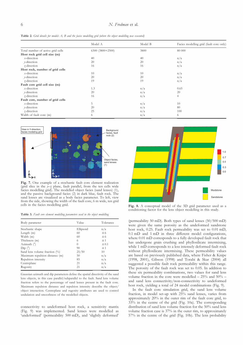
The stochastic facies modelling was executed using a stan-dard object-based (Haldorsen & Damsleth 1990; Wietzerbin& Mallet 1994) facies modelling tool, the Facies:Compositemodule in RMS, originally developed for a wide range ofsedimentary facies modelling purposes. In this study, however,the module was used in a non-standard fashion, to model faultcore architecture. For modelling purposes, the sand lensesserved as the simulated object facies and the fault rock servedas the passive ‘background’ facies (Fig. 7). The sand lenses weremodelled as ellipsoids, and their body geometry defined by anumber of Gaussian parameters (Table 3). A continuous 3Dgrid parameter (Fig. 8) was used as a conditioning factor for thesand lens object modelling; it describes the spatial probabilitydistribution of lenses as a linear function with a maximum valueat the centre of the fault core and decreasing outwards, but iskept constant along fault strike.

In order to investigate the sensitivity of fluid flow topetrophysical properties, sand lens fraction and sand lens

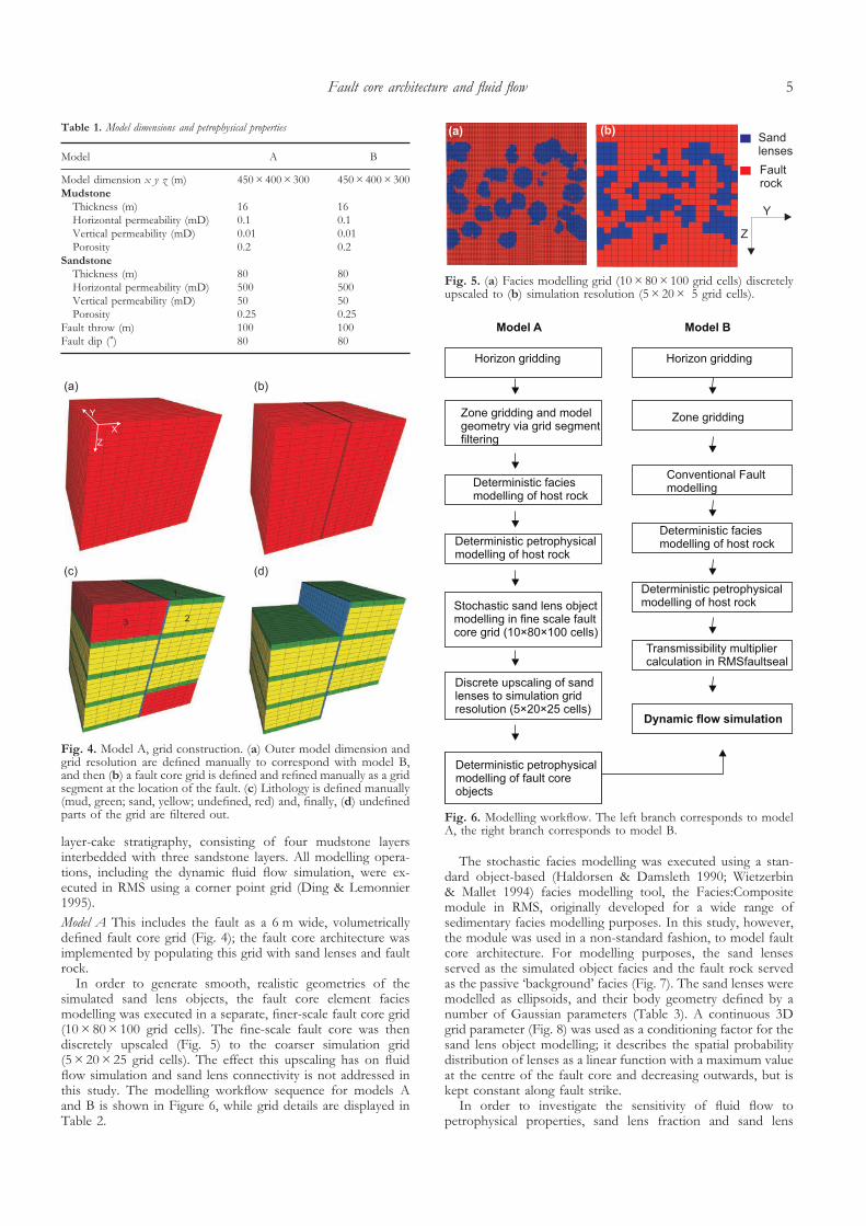
Table 1. Model dimensions and petrophysical properties

Model A B

Model dimension x y z (m) 450�400�300 450�400�300Mudstone

Thickness (m) 16 16Horizontal permeability (mD) 0.1 0.1Vertical permeability (mD) 0.01 0.01Porosity 0.2 0.2

Sandstone

Thickness (m) 80 80Horizontal permeability (mD) 500 500Vertical permeability (mD) 50 50Porosity 0.25 0.25

Fault throw (m) 100 100Fault dip (�) 80 80

Fig. 4. Model A, grid construction. (a) Outer model dimension andgrid resolution are defined manually to correspond with model B,and then (b) a fault core grid is defined and refined manually as a gridsegment at the location of the fault. (c) Lithology is defined manually(mud, green; sand, yellow; undefined, red) and, finally, (d) undefinedparts of the grid are filtered out.

Fig. 5. (a) Facies modelling grid (10�80�100 grid cells) discretelyupscaled to (b) simulation resolution (5�20� 5 grid cells).

Fig. 6. Modelling workflow. The left branch corresponds to modelA, the right branch corresponds to model B.

Fault core architecture and fluid flow 5

connectivity to undeformed host rock, a sensitivity matrix(Fig. 9) was implemented. Sand lenses were modelled as‘undeformed’ (permeability 500 mD), and ‘slightly deformed’

(permeability 50 mD). Both types of sand lenses (50/500 mD)were given the same porosity as the undeformed sandstonehost rock, 0.25. Fault rock permeability was set to 0.01 mD,0.1 mD and 1 mD in three different model configurations,where 0.01 mD corresponds to a fully developed fault rock thathas undergone grain crushing and phyllosilicate intermixing,while 1 mD corresponds to a less intensely deformed fault rockwithout phyllosilicate intermixing. These permeability valuesare based on previously published data, where Fisher & Knipe(1998, 2001), Gibson (1998) and Torabi & Skar (2004) allsuggested a possible fault rock permeability within this range.The porosity of the fault rock was set to 0.05. In addition tothese six permeability combinations, two values for sand lensvolume fraction in the core were modelled – 25% and 50% –and sand lens connectivity/non-connectivity to undeformedhost rock, yielding a total of 24 model combinations (Fig. 9).

In the fault core simulation grid, the sand lens volumefraction, in model set-up with 25% sand lenses, varies fromapproximately 20% in the outer rim of the fault core grid, to33% in the centre of the grid (Fig. 10a). The correspondingdistribution of sand lens volume fraction for the 50% sand lensvolume fraction case is 37% in the outer rim, to approximately57% in the centre of the grid (Fig. 10b). The lens probability

Table 2. Grid details for models A, B and the facies modelling grid (where the object modelling was executed)

Model A Model B Facies modelling grid (fault core only)

Total number of active grid cells 6300 (3800+2500) 3800 80 000Host rock grid cell size (m)

x-direction 40 40 n/ay-direction 20 20 n/az-direction 16 16 n/a

Host rock, number of grid cells

x-direction 10 10 n/ay-direction 20 20 n/az-direction 19 19 n/a

Fault core grid cell size (m)

x-direction 1.3 n/a 0.65y-direction 20 n/a 20z-direction 16 n/a 4

Fault core, number of grid cells

x-direction 5 n/a 10y-direction 20 n/a 80z-direction 25 n/a 100

Width of fault core (m) 6 n/a 6

Fig. 7. One example of a stochastic fault core element realization(grid slice in the y–z plane, fault parallel, from the ten cells widefacies modelling grid). The modelled object facies (sand lenses) (1),and the passive background facies (2) in dark blue, fault rock. Thesand lenses are visualized as a body facies parameter. To left, viewfrom the side, showing the width of the fault core, 6 m wide, ten gridcells in the facies modelling grid.

Table 3. Fault core element modelling parameters used in the object modelling

Body parameter Value Tolerance

Stochastic shape Ellipsoid n/aLength (m) 60 �6Width (m) 60 �6Thickness (m) 6 �1Azimuth (�) 0 �0.1Dip (�) 90 �1Sand lens volume fraction (%) 25/50 10Maximum repulsion distance (m) 50 n/aRepulsion intensity 85 n/aCentreplane 21 n/aRugosity 21 n/a

Gaussian azimuth and dip parameters define the spatial directivity of the sandlens objects, in this case parallel/subparallel to the fault. Sand lens volumefraction refers to the percentage of sand lenses present in the fault core.Maximum repulsion distance and repulsion intensity describe the object/object interaction. Centreplane and rugosity attributes are used to controlundulation and smoothness of the modelled objects.

Fig. 8. A conceptual model of the 3D grid parameter used as aconditioning factor for the lens object modelling in this study.

N. Fredman et al.6

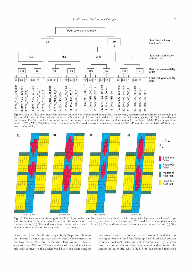
factor (Fig. 8) and the ellipsoid object body shape contribute tothe outwards decreasing body density trend. Consequently, inthe two cases, 25% and 50% sand lens volume fraction,approximately 20% and 37% respectively of the sand lens faciesgrid cells connect to the undeformed host rock (sandstone or

mudstone). Sand lens connectivity to host rock is defined ashaving at least one sand lens facies grid cell in physical contactwith one host rock facies grid cell. Non-connectivity betweenhost rock and sand lenses was implemented by deterministicallysetting the outer grid cells (1/5, 5/5) to background fault rock

Fig. 9. Model A. Fluid flow sensitivity analyses on sand lens volume fraction, sand lens connectivity, and permeability were set up according tothis sensitivity matrix. Each of the bottom combinations (1–24) was executed in 20 stochastic realizations, giving 480 fault core elementrealizations. The 24 combinations are text coded according to the boxes in the matrix and are referred to as ‘flow models’. For example, flowmodel 1 (25%_YES_500_0.01) refers to a model with 25% sand lens volume fraction, connected 500 mD sand lenses, and 0.01 mD fault rockmatrix permeability.

Fig. 10. The fault core simulation grid (5�20�25 grid cells) seen from the side (x–z plane), which conceptually illustrates the ellipsoid shapeand distribution of the sand lens bodies, and the concept of connected/unconnected sand lenses. (a) 25% sand lens volume fraction withconnected lenses; (b) 50% sand lens volume fraction with connected lenses. (c) 25% sand lens volume fraction with unconnected lenses; (d) 50%sand lens volume fraction with unconnected sand lenses.

Fault core architecture and fluid flow 7

facies (Figs 10c, 10d). A direct consequence of this modifica-tion is a reduction of the number of sand lens facies grid cellsthat are present in the fault core. The ‘25% lens fraction’ casewith unconnected cells now actually contains approximately19%, and the ‘50% lens fraction’ case approximately 32% sandlens facies cells in the fault core.Model B The fault in model B was implemented with faulttransmissibility multipliers (Manzocchi et al. 1999). The faulttransmissibility multipliers were calculated with equation (3)(Roxar 2005), where Tmult is the fault transmissibility multiplier,Wfz is the fault zone thickness (m), kfw is the footwall gridblock permeability (mD), khw is the hanging-wall grid blockpermeability (mD), L is the grid cell dimension (m) and kfz isthe fault zone permeability (mD):

Tmult =� 1kfw

+ 1khw

�

��1 � �Wfz

L��

kfw

+�1 � �Wfz

L��

khw

+

�2Wfz�

Lkfz

�(3)

The fault zone permeability, kfz, was calculated using equa-tion (2). In the study, however, the effect of including sandlenses in model A with respect to simulation response is beinginvestigated, so the fault zone permeability, kfz, in model B,must correspond to the fault rock matrix permeability in modelA. In that way it is possible to evaluate sand lens impact onfluid flow. The matching of kfz to the fault rock permeabilityrequires three values for kfz, 0.01 mD, 0.1 mD and 1 mD,which were achieved by the use of a Vshale parameter, incombination with a multiplier called ‘brittle factor’ (Roxar2005). Vshale is the mud fraction in every grid cell, and the brittlefactor is a deterministic multiplier between 1 and 100, whichoperates uniformly on the entire fault plane and directly on thefault zone permeability, kfz. The idea behind the brittle factor isthat brittle deformation by cataclasis and/or brecciation mayinitiate cracks and microfractures, and actually increase the porespace, thus increasing the effective permeability (Roxar 2005).For the present lithology, equation (2) calculates the fault zonepermeability, kfz, to approximately 0.14 mD (SGR=0.16–0.18 ,D=100 m). Subsequently, Vshale and brittle factor were usedtogether to adjust 0.14 to the matching values of 0.01 mD,0.1 mD and 1 mD.

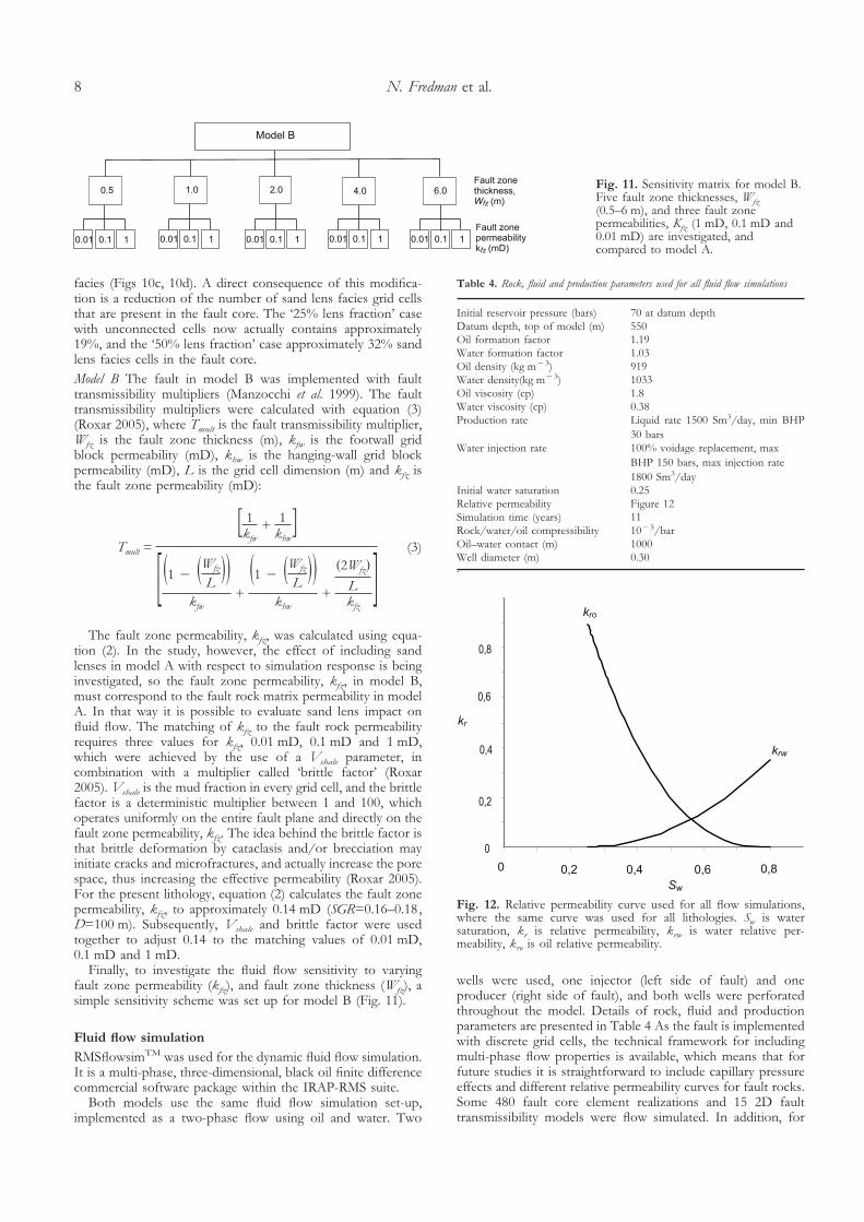
Finally, to investigate the fluid flow sensitivity to varyingfault zone permeability (kfz), and fault zone thickness (Wfz), asimple sensitivity scheme was set up for model B (Fig. 11).

Fluid flow simulation

RMSflowsimTM was used for the dynamic fluid flow simulation.It is a multi-phase, three-dimensional, black oil finite differencecommercial software package within the IRAP-RMS suite.

Both models use the same fluid flow simulation set-up,implemented as a two-phase flow using oil and water. Two

wells were used, one injector (left side of fault) and oneproducer (right side of fault), and both wells were perforatedthroughout the model. Details of rock, fluid and productionparameters are presented in Table 4 As the fault is implementedwith discrete grid cells, the technical framework for includingmulti-phase flow properties is available, which means that forfuture studies it is straightforward to include capillary pressureeffects and different relative permeability curves for fault rocks.Some 480 fault core element realizations and 15 2D faulttransmissibility models were flow simulated. In addition, for

Fig. 11. Sensitivity matrix for model B.Five fault zone thicknesses, Wfz

(0.5–6 m), and three fault zonepermeabilities, Kfz (1 mD, 0.1 mD and0.01 mD) are investigated, andcompared to model A.

Table 4. Rock, fluid and production parameters used for all fluid flow simulations

Initial reservoir pressure (bars) 70 at datum depthDatum depth, top of model (m) 550Oil formation factor 1.19Water formation factor 1.03Oil density (kg m�3) 919Water density(kg m�3) 1033Oil viscosity (cp) 1.8Water viscosity (cp) 0.38Production rate Liquid rate 1500 Sm3/day, min BHP

30 barsWater injection rate 100% voidage replacement, max

BHP 150 bars, max injection rate1800 Sm3/day

Initial water saturation 0.25Relative permeability Figure 12Simulation time (years) 11Rock/water/oil compressibility 10�5/barOil–water contact (m) 1000Well diameter (m) 0.30.

Fig. 12. Relative permeability curve used for all flow simulations,where the same curve was used for all lithologies. Sw is watersaturation, kr is relative permeability, krw is water relative per-meability, kro is oil relative permeability.

N. Fredman et al.8

reasons of comparison, three additional fault core elementmodels with uniform fault core permeability (1 mD, 0.1 mDand 0.01 mD) were flow simulated, giving a total of 498 flowsimulated models.

FLUID FLOW SIMULATION RESULTS

All fluid flow simulations were run for 4018 days. Monitoredparameters include oil recovery, mean injection well bottom

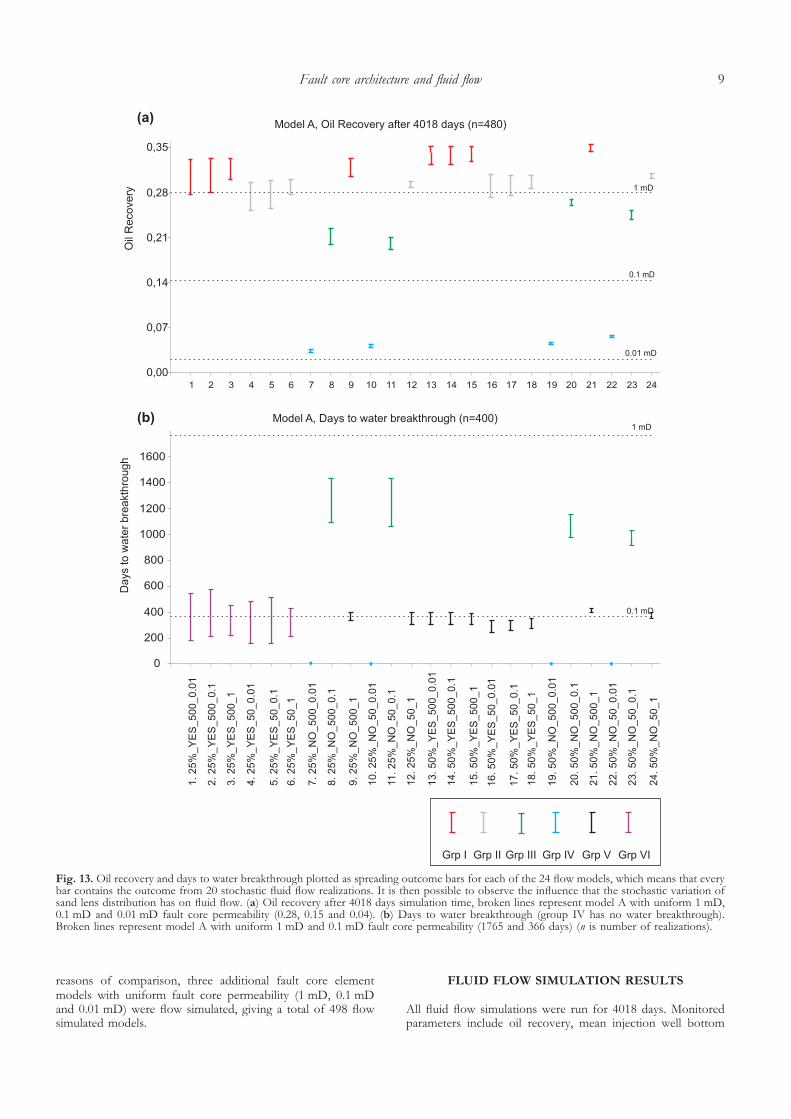
Fig. 13. Oil recovery and days to water breakthrough plotted as spreading outcome bars for each of the 24 flow models, which means that everybar contains the outcome from 20 stochastic fluid flow realizations. It is then possible to observe the influence that the stochastic variation ofsand lens distribution has on fluid flow. (a) Oil recovery after 4018 days simulation time, broken lines represent model A with uniform 1 mD,0.1 mD and 0.01 mD fault core permeability (0.28, 0.15 and 0.04). (b) Days to water breakthrough (group IV has no water breakthrough).Broken lines represent model A with uniform 1 mD and 0.1 mD fault core permeability (1765 and 366 days) (n is number of realizations).

Fault core architecture and fluid flow 9

hole pressure (BHP), days to water breakthrough, and watercut. Simulation response for five fault core parameters wasinvestigated: (p1) sand lens volume fraction; (p2) connectivitybetween sand lenses and undeformed host rock; (p3) sand lenspermeability; (p4) stochastic distribution of sand lenses; (p5)fault rock matrix permeability.

Figure 13a shows oil recovery at the end of simulation after4018 days, while Figure 13b shows days to water breakthrough.Results from Figures 14 and 15 facilitate a subdivision of the 24flow models based on oil recovery and days to water break-through into six groups – I, II, III, IV, V and VI – eachhighlighted with a different colour. The first four groups (I–IV)

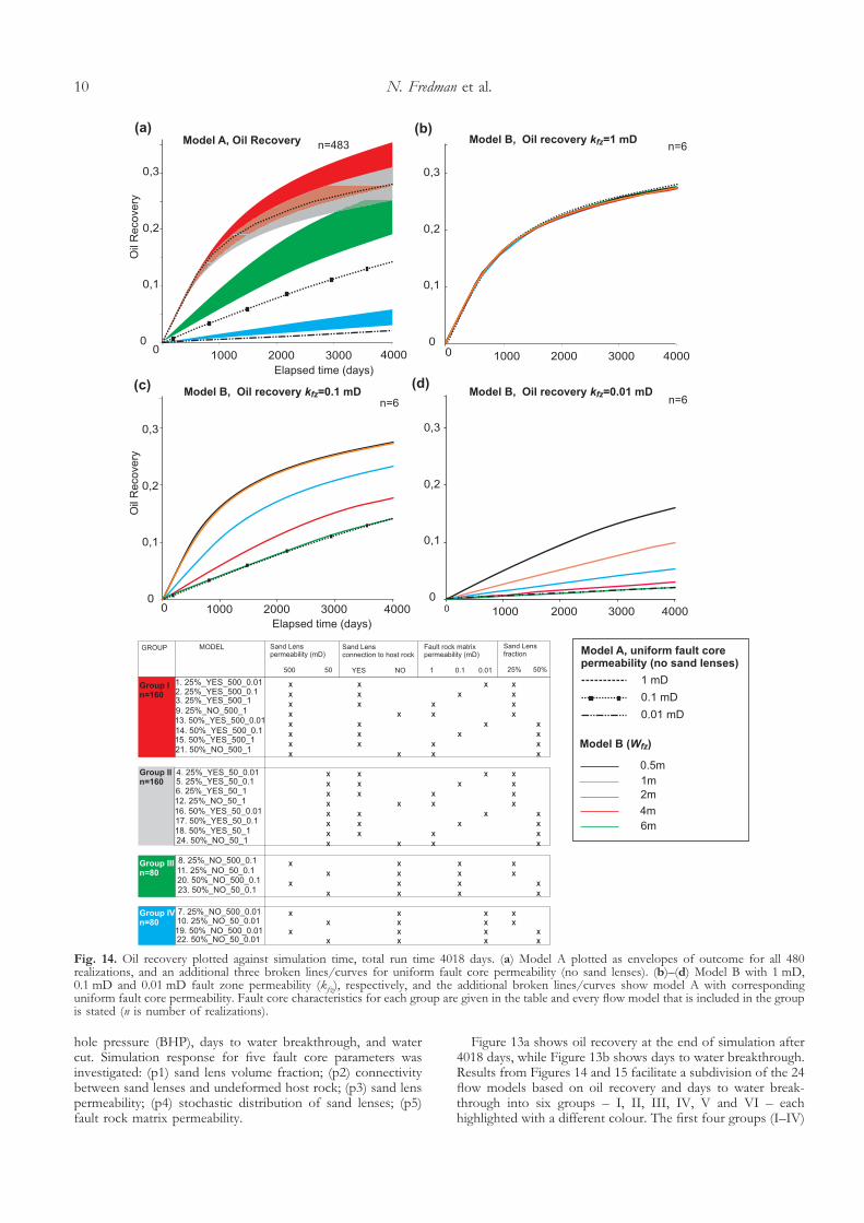
Fig. 14. Oil recovery plotted against simulation time, total run time 4018 days. (a) Model A plotted as envelopes of outcome for all 480realizations, and an additional three broken lines/curves for uniform fault core permeability (no sand lenses). (b)–(d) Model B with 1 mD,0.1 mD and 0.01 mD fault zone permeability (kfz), respectively, and the additional broken lines/curves show model A with correspondinguniform fault core permeability. Fault core characteristics for each group are given in the table and every flow model that is included in the groupis stated (n is number of realizations).

N. Fredman et al.10

are distinguished based on oil recovery and the last two groups(V–VI) on the basis of days to water breakthrough. Thesubdivision of the groups is summarized in Table 5; they canalso be identified in Figure 13.

Figures 14 and 15 show oil recovery and water cut over timefor models A and B. The spread of simulation responses for the

six groups, shown as coloured sectors (outcome envelopes),indicates the total spread of all model realizations over time foreach group. Three separate simulations with uniform fault corepermeability (no sand lenses) for model A are shown in Figures13, 14 and 15 as ‘uniform fault core permeability’. Figures14b–d, 15b–d show oil recovery and water cut for model B

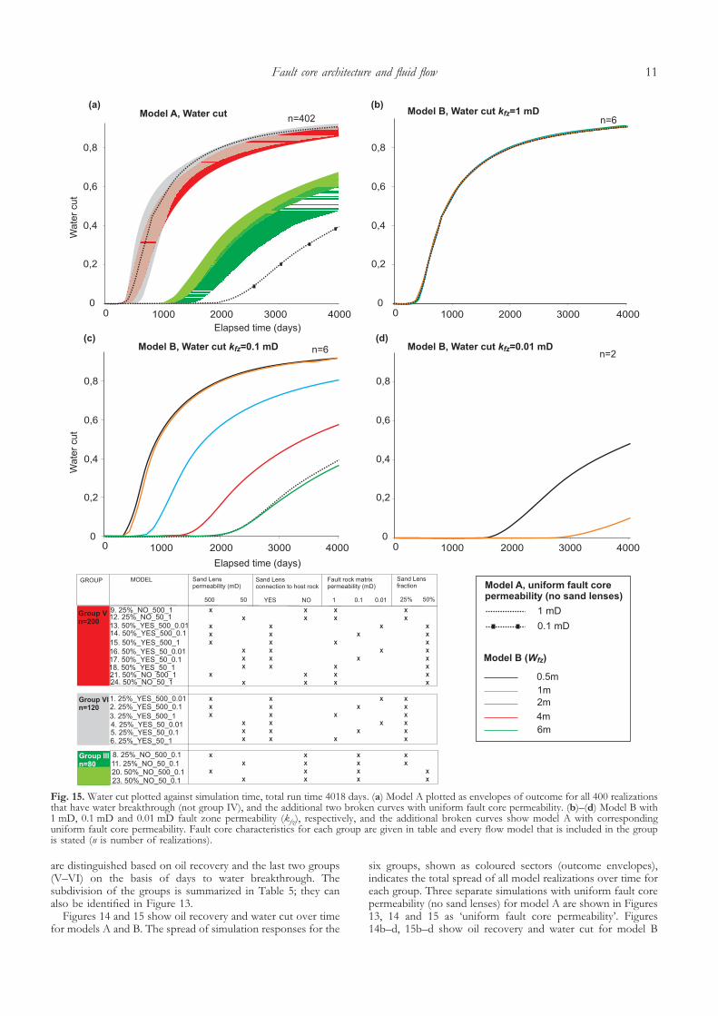
Fig. 15. Water cut plotted against simulation time, total run time 4018 days. (a) Model A plotted as envelopes of outcome for all 400 realizationsthat have water breakthrough (not group IV), and the additional two broken curves with uniform fault core permeability. (b)–(d) Model B with1 mD, 0.1 mD and 0.01 mD fault zone permeability (kfz), respectively, and the additional broken curves show model A with correspondinguniform fault core permeability. Fault core characteristics for each group are given in table and every flow model that is included in the groupis stated (n is number of realizations).

Fault core architecture and fluid flow 11

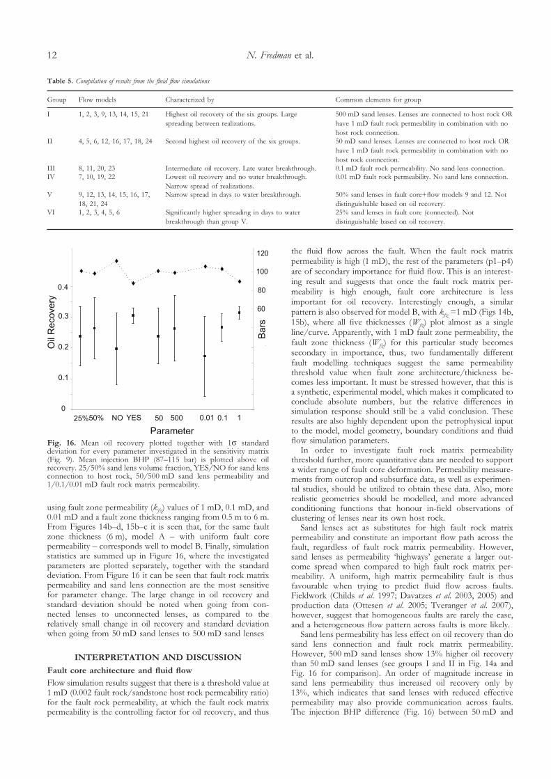
using fault zone permeability (kfz) values of 1 mD, 0.1 mD, and0.01 mD and a fault zone thickness ranging from 0.5 m to 6 m.From Figures 14b–d, 15b–c it is seen that, for the same faultzone thickness (6 m), model A – with uniform fault corepermeability – corresponds well to model B. Finally, simulationstatistics are summed up in Figure 16, where the investigatedparameters are plotted separately, together with the standarddeviation. From Figure 16 it can be seen that fault rock matrixpermeability and sand lens connection are the most sensitivefor parameter change. The large change in oil recovery andstandard deviation should be noted when going from con-nected lenses to unconnected lenses, as compared to therelatively small change in oil recovery and standard deviationwhen going from 50 mD sand lenses to 500 mD sand lenses

INTERPRETATION AND DISCUSSION

Fault core architecture and fluid flow

Flow simulation results suggest that there is a threshold value at1 mD (0.002 fault rock/sandstone host rock permeability ratio)for the fault rock permeability, at which the fault rock matrixpermeability is the controlling factor for oil recovery, and thus

the fluid flow across the fault. When the fault rock matrixpermeability is high (1 mD), the rest of the parameters (p1–p4)are of secondary importance for fluid flow. This is an interest-ing result and suggests that once the fault rock matrix per-meability is high enough, fault core architecture is lessimportant for oil recovery. Interestingly enough, a similarpattern is also observed for model B, with kfz =1 mD (Figs 14b,15b), where all five thicknesses (Wfz) plot almost as a singleline/curve. Apparently, with 1 mD fault zone permeability, thefault zone thickness (Wfz) for this particular study becomessecondary in importance, thus, two fundamentally differentfault modelling techniques suggest the same permeabilitythreshold value when fault zone architecture/thickness be-comes less important. It must be stressed however, that this isa synthetic, experimental model, which makes it complicated toconclude absolute numbers, but the relative differences insimulation response should still be a valid conclusion. Theseresults are also highly dependent upon the petrophysical inputto the model, model geometry, boundary conditions and fluidflow simulation parameters.

In order to investigate fault rock matrix permeabilitythreshold further, more quantitative data are needed to supporta wider range of fault core deformation. Permeability measure-ments from outcrop and subsurface data, as well as experimen-tal studies, should be utilized to obtain these data. Also, morerealistic geometries should be modelled, and more advancedconditioning functions that honour in-field observations ofclustering of lenses near its own host rock.

Sand lenses act as substitutes for high fault rock matrixpermeability and constitute an important flow path across thefault, regardless of fault rock matrix permeability. However,sand lenses as permeability ‘highways’ generate a larger out-come spread when compared to high fault rock matrix per-meability. A uniform, high matrix permeability fault is thusfavourable when trying to predict fluid flow across faults.Fieldwork (Childs et al. 1997; Davatzes et al. 2003, 2005) andproduction data (Ottesen et al. 2005; Tveranger et al. 2007),however, suggest that homogeneous faults are rarely the case,and a heterogeneous flow pattern across faults is more likely.

Sand lens permeability has less effect on oil recovery than dosand lens connection and fault rock matrix permeability.However, 500 mD sand lenses show 13% higher oil recoverythan 50 mD sand lenses (see groups I and II in Fig. 14a andFig. 16 for comparison). An order of magnitude increase insand lens permeability thus increased oil recovery only by13%, which indicates that sand lenses with reduced effectivepermeability may also provide communication across faults.The injection BHP difference (Fig. 16) between 50 mD and

Table 5. Compilation of results from the fluid flow simulations

Group Flow models Characterized by Common elements for group

I 1, 2, 3, 9, 13, 14, 15, 21 Highest oil recovery of the six groups. Largespreading between realizations.

500 mD sand lenses. Lenses are connected to host rock ORhave 1 mD fault rock permeability in combination with nohost rock connection.

II 4, 5, 6, 12, 16, 17, 18, 24 Second highest oil recovery of the six groups. 50 mD sand lenses. Lenses are connected to host rock ORhave 1 mD fault rock permeability in combination with nohost rock connection.

III 8, 11, 20, 23 Intermediate oil recovery. Late water breakthrough. 0.1 mD fault rock permeability. No sand lens connection.IV 7, 10, 19, 22 Lowest oil recovery and no water breakthrough.

Narrow spread of realizations.0.01 mD fault rock permeability. No sand lens connection.

V 9, 12, 13, 14, 15, 16, 17,18, 21, 24

Narrow spread in days to water breakthrough. 50% sand lenses in fault core+flow models 9 and 12. Notdistinguishable based on oil recovery.

VI 1, 2, 3, 4, 5, 6 Significantly higher spreading in days to waterbreakthrough than group V.

25% sand lenses in fault core (connected). Notdistinguishable based on oil recovery.

Fig. 16. Mean oil recovery plotted together with 1� standarddeviation for every parameter investigated in the sensitivity matrix(Fig. 9). Mean injection BHP (87–115 bar) is plotted above oilrecovery. 25/50% sand lens volume fraction, YES/NO for sand lensconnection to host rock, 50/500 mD sand lens permeability and1/0.1/0.01 mD fault rock matrix permeability.

N. Fredman et al.12

500 mD sand lenses is also minor, which further supports thisconclusion.

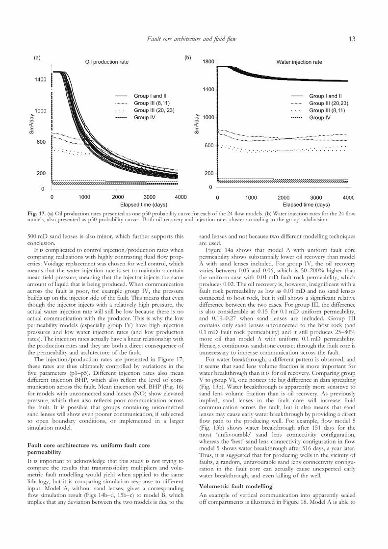
It is complicated to control injection/production rates whencomparing realizations with highly contrasting fluid flow prop-erties. Voidage replacement was chosen for well control, whichmeans that the water injection rate is set to maintain a certainmean field pressure, meaning that the injector injects the sameamount of liquid that is being produced. When communicationacross the fault is poor, for example group IV, the pressurebuilds up on the injector side of the fault. This means that eventhough the injector injects with a relatively high pressure, theactual water injection rate will still be low because there is noactual communication with the producer. This is why the lowpermeability models (especially group IV) have high injectionpressures and low water injection rates (and low productionrates). The injection rates actually have a linear relationship withthe production rates and they are both a direct consequence ofthe permeability and architecture of the fault.

The injection/production rates are presented in Figure 17;these rates are thus ultimately controlled by variations in thefive parameters (p1–p5). Different injection rates also meandifferent injection BHP, which also reflect the level of com-munication across the fault. Mean injection well BHP (Fig. 16)for models with unconnected sand lenses (NO) show elevatedpressure, which then also reflects poor communication acrossthe fault. It is possible that groups containing unconnectedsand lenses will show even poorer communication, if subjectedto open boundary conditions, or implemented in a largersimulation model.

Fault core architecture vs. uniform fault corepermeability

It is important to acknowledge that this study is not trying tocompare the results that transmissibility multipliers and volu-metric fault modelling would yield when applied to the samelithology, but it is comparing simulation response to differentinput. Model A, without sand lenses, gives a correspondingflow simulation result (Figs 14b–d, 15b–c) to model B, whichimplies that any deviation between the two models is due to the

sand lenses and not because two different modelling techniquesare used.

Figure 14a shows that model A with uniform fault corepermeability shows substantially lower oil recovery than modelA with sand lenses included. For group IV, the oil recoveryvaries between 0.03 and 0.06, which is 50–200% higher thanthe uniform case with 0.01 mD fault rock permeability, whichproduces 0.02. The oil recovery is, however, insignificant with afault rock permeability as low as 0.01 mD and no sand lensesconnected to host rock, but it still shows a significant relativedifference between the two cases. For group III, the differenceis also considerable at 0.15 for 0.1 mD uniform permeability,and 0.19–0.27 when sand lenses are included. Group IIIcontains only sand lenses unconnected to the host rock (and0.1 mD fault rock permeability) and it still produces 25–80%more oil than model A with uniform 0.1 mD permeability.Hence, a continuous sandstone contact through the fault core isunnecessary to increase communication across the fault.

For water breakthrough, a different pattern is observed, andit seems that sand lens volume fraction is more important forwater breakthrough than it is for oil recovery. Comparing groupV to group VI, one notices the big difference in data spreading(Fig. 13b). Water breakthrough is apparently more sensitive tosand lens volume fraction than is oil recovery. As previouslyimplied, sand lenses in the fault core will increase fluidcommunication across the fault, but it also means that sandlenses may cause early water breakthrough by providing a directflow path to the producing well. For example, flow model 5(Fig. 13b) shows water breakthrough after 151 days for themost ‘unfavourable’ sand lens connectivity configuration,whereas the ‘best’ sand lens connectivity configuration in flowmodel 5 shows water breakthrough after 516 days, a year later.Thus, it is suggested that for producing wells in the vicinity offaults, a random, unfavourable sand lens connectivity configu-ration in the fault core can actually cause unexpected earlywater breakthrough, and even killing of the well.

Volumetric fault modelling

An example of vertical communication into apparently sealedoff compartments is illustrated in Figure 18. Model A is able to

Fig. 17. (a) Oil production rates presented as one p50 probability curve for each of the 24 flow models. (b) Water injection rates for the 24 flowmodels, also presented as p50 probability curves. Both oil recovery and injection rates cluster according to the group subdivision.

Fault core architecture and fluid flow 13

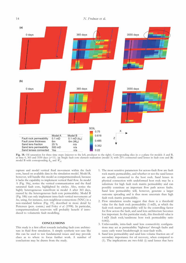
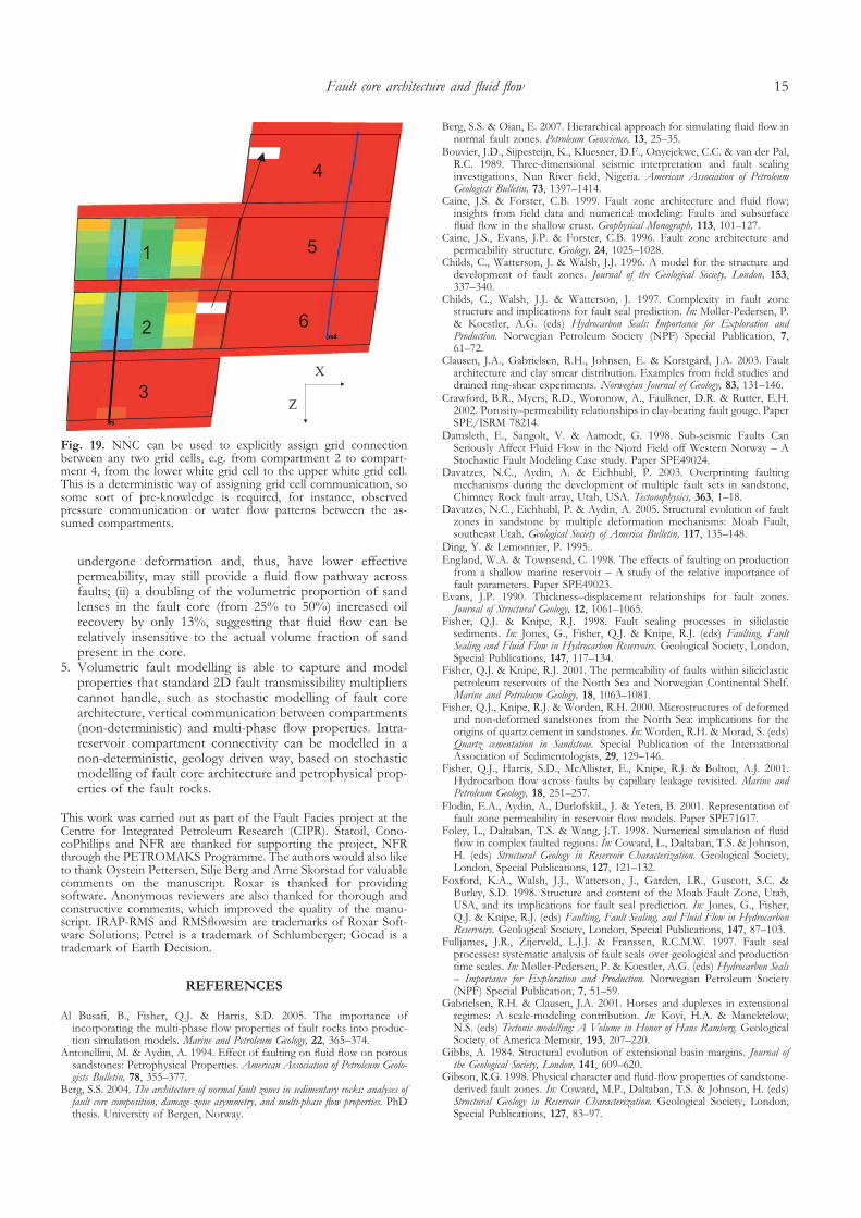
capture and model vertical fluid movement within the faultcore, based on available data in the simulation model. Model B,however, will handle this model as compartmentalized, becauseit lacks the capability to implement vertical fluid flow. In modelA (Fig. 18a), notice the vertical communication and the fluidsaturated fault core, highlighted by circles. Also, notice thehighly heterogeneous waterfront in model A after 365 days,caused by the heterogeneous fault core permeability. Model B(Fig. 18b) can only implement intra-fault vertical movements adhoc, using, for instance, non-neighbour-connections (NNC) in anon-standard fashion (Fig. 19), described in more detail byPettersen (pers. comm.) and Foley et al. (1998). In particular,compartmentalized reservoirs will probably benefit if intro-duced to volumetric fault modelling.

CONCLUSIONS

This study is a first effort towards including fault core architec-ture in fluid flow simulation. A simple synthetic test case likethis can be used to test fundamental issues and may provideclues as to where to focus further work. A number ofconclusions may be drawn from the study.

1. The most sensitive parameters for across-fault flow are faultrock matrix permeability, and whether or not the sand lensesare actually connected to the host rock. Sand lenses inphysical connection with undeformed host rock may be asubstitute for high fault rock matrix permeability and canpossibly constitute an important flow path across faults.Sand lens permeability will, however, generate a largeroutcome spreading and is thus more uncertain than highfault rock matrix permeability.

2. Flow simulation results suggest that there is a thresholdvalue for the fault rock permeability (1 mD), at which thefault rock matrix permeability will be the controlling factorfor flow across the fault, and sand lens architecture becomesless important. In this particular study, this threshold value is1 mD (fault rock/sandstone host rock permeability ratio0.002).

3. Unfavourable, intra-fault sand lens connectivity configura-tions may act as permeability ‘highways’ through faults andcause early water breakthrough in near-fault wells.

4. Sand lens permeability and sand lens volume fraction are ofsecondary importance for oil recovery, when compared to(1). The implications are two-fold: (i) sand lenses that have

Fig. 18. Oil saturation for three time steps (injector to the left, producer to the right). Corresponding slice in x–z plane for models A and B,at time 0, 365 and 3550 days (y=11). (a) Single fault core element realization (model A) with 25% connected sand lenses in fault core and (b)model B with corresponding kfz and Wfz.

N. Fredman et al.14

undergone deformation and, thus, have lower effectivepermeability, may still provide a fluid flow pathway acrossfaults; (ii) a doubling of the volumetric proportion of sandlenses in the fault core (from 25% to 50%) increased oilrecovery by only 13%, suggesting that fluid flow can berelatively insensitive to the actual volume fraction of sandpresent in the core.

5. Volumetric fault modelling is able to capture and modelproperties that standard 2D fault transmissibility multiplierscannot handle, such as stochastic modelling of fault corearchitecture, vertical communication between compartments(non-deterministic) and multi-phase flow properties. Intra-reservoir compartment connectivity can be modelled in anon-deterministic, geology driven way, based on stochasticmodelling of fault core architecture and petrophysical prop-erties of the fault rocks.

This work was carried out as part of the Fault Facies project at theCentre for Integrated Petroleum Research (CIPR). Statoil, Cono-coPhillips and NFR are thanked for supporting the project, NFRthrough the PETROMAKS Programme. The authors would also liketo thank Øystein Pettersen, Silje Berg and Arne Skorstad for valuablecomments on the manuscript. Roxar is thanked for providingsoftware. Anonymous reviewers are also thanked for thorough andconstructive comments, which improved the quality of the manu-script. IRAP-RMS and RMSflowsim are trademarks of Roxar Soft-ware Solutions; Petrel is a trademark of Schlumberger; Gocad is atrademark of Earth Decision.

REFERENCES

Al Busafi, B., Fisher, Q.J. & Harris, S.D. 2005. The importance ofincorporating the multi-phase flow properties of fault rocks into produc-tion simulation models. Marine and Petroleum Geology, 22, 365–374.

Antonellini, M. & Aydin, A. 1994. Effect of faulting on fluid flow on poroussandstones: Petrophysical Properties. American Association of Petroleum Geolo-gists Bulletin, 78, 355–377.

Berg, S.S. 2004. The architecture of normal fault zones in sedimentary rocks: analyses offault core composition, damage zone asymmetry, and multi-phase flow properties. PhDthesis. University of Bergen, Norway.

Berg, S.S. & Øian, E. 2007. Hierarchical approach for simulating fluid flow innormal fault zones. Petroleum Geoscience, 13, 25–35.

Bouvier, J.D., Sijpesteijn, K., Kluesner, D.F., Onyejekwe, C.C. & van der Pal,R.C. 1989. Three-dimensional seismic interpretation and fault sealinginvestigations, Nun River field, Nigeria. American Association of PetroleumGeologists Bulletin, 73, 1397–1414.

Caine, J.S. & Forster, C.B. 1999. Fault zone architecture and fluid flow;insights from field data and numerical modeling: Faults and subsurfacefluid flow in the shallow crust. Geophysical Monograph, 113, 101–127.

Caine, J.S., Evans, J.P. & Forster, C.B. 1996. Fault zone architecture andpermeability structure. Geology, 24, 1025–1028.

Childs, C., Watterson, J. & Walsh, J.J. 1996. A model for the structure anddevelopment of fault zones. Journal of the Geological Society, London, 153,337–340.

Childs, C., Walsh, J.J. & Watterson, J. 1997. Complexity in fault zonestructure and implications for fault seal prediction. In: Møller-Pedersen, P.& Koestler, A.G. (eds) Hydrocarbon Seals: Importance for Exploration andProduction. Norwegian Petroleum Society (NPF) Special Publication, 7,61–72.

Clausen, J.A., Gabrielsen, R.H., Johnsen, E. & Korstgård, J.A. 2003. Faultarchitecture and clay smear distribution. Examples from field studies anddrained ring-shear experiments. Norwegian Journal of Geology, 83, 131–146.

Crawford, B.R., Myers, R.D., Woronow, A., Faulkner, D.R. & Rutter, E.H.2002. Porosity–permeability relationships in clay-bearing fault gouge. PaperSPE/ISRM 78214.

Damsleth, E., Sangolt, V. & Aamodt, G. 1998. Sub-seismic Faults CanSeriously Affect Fluid Flow in the Njord Field off Western Norway – AStochastic Fault Modeling Case study. Paper SPE49024.

Davatzes, N.C., Aydin, A. & Eichhubl, P. 2003. Overprinting faultingmechanisms during the development of multiple fault sets in sandstone,Chimney Rock fault array, Utah, USA. Tectonophysics, 363, 1–18.

Davatzes, N.C., Eichhubl, P. & Aydin, A. 2005. Structural evolution of faultzones in sandstone by multiple deformation mechanisms: Moab Fault,southeast Utah. Geological Society of America Bulletin, 117, 135–148.

Ding, Y. & Lemonnier, P. 1995..England, W.A. & Townsend, C. 1998. The effects of faulting on production

from a shallow marine reservoir – A study of the relative importance offault parameters. Paper SPE49023.

Evans, J.P. 1990. Thickness–displacement relationships for fault zones.Journal of Structural Geology, 12, 1061–1065.

Fisher, Q.J. & Knipe, R.J. 1998. Fault sealing processes in siliclasticsediments. In: Jones, G., Fisher, Q.J. & Knipe, R.J. (eds) Faulting, FaultSealing and Fluid Flow in Hydrocarbon Reservoirs. Geological Society, London,Special Publications, 147, 117–134.

Fisher, Q.J. & Knipe, R.J. 2001. The permeability of faults within siliciclasticpetroleum reservoirs of the North Sea and Norwegian Continental Shelf.Marine and Petroleum Geology, 18, 1063–1081.

Fisher, Q.J., Knipe, R.J. & Worden, R.H. 2000. Microstructures of deformedand non-deformed sandstones from the North Sea: implications for theorigins of quartz cement in sandstones. In: Worden, R.H. & Morad, S. (eds)Quartz cementation in Sandstone. Special Publication of the InternationalAssociation of Sedimentologists, 29, 129–146.

Fisher, Q.J., Harris, S.D., McAllister, E., Knipe, R.J. & Bolton, A.J. 2001.Hydrocarbon flow across faults by capillary leakage revisited. Marine andPetroleum Geology, 18, 251–257.

Flodin, E.A., Aydin, A., DurlofskiL, J. & Yeten, B. 2001. Representation offault zone permeability in reservoir flow models. Paper SPE71617.

Foley, L., Daltaban, T.S. & Wang, J.T. 1998. Numerical simulation of fluidflow in complex faulted regions. In: Coward, L., Daltaban, T.S. & Johnson,H. (eds) Structural Geology in Reservoir Characterization. Geological Society,London, Special Publications, 127, 121–132.

Foxford, K.A., Walsh, J.J., Watterson, J., Garden, I.R., Guscott, S.C. &Burley, S.D. 1998. Structure and content of the Moab Fault Zone, Utah,USA, and its implications for fault seal prediction. In: Jones, G., Fisher,Q.J. & Knipe, R.J. (eds) Faulting, Fault Sealing, and Fluid Flow in HydrocarbonReservoirs. Geological Society, London, Special Publications, 147, 87–103.

Fulljames, J.R., Zijerveld, L.J.J. & Franssen, R.C.M.W. 1997. Fault sealprocesses: systematic analysis of fault seals over geological and productiontime scales. In: Møller-Pedersen, P. & Koestler, A.G. (eds) Hydrocarbon Seals– Importance for Exploration and Production. Norwegian Petroleum Society(NPF) Special Publication, 7, 51–59.

Gabrielsen, R.H. & Clausen, J.A. 2001. Horses and duplexes in extensionalregimes: A scale-modeling contribution. In: Koyi, H.A. & Mancktelow,N.S. (eds) Tectonic modelling: A Volume in Honor of Hans Ramberg. GeologicalSociety of America Memoir, 193, 207–220.

Gibbs, A. 1984. Structural evolution of extensional basin margins. Journal ofthe Geological Society, London, 141, 609–620.

Gibson, R.G. 1998. Physical character and fluid-flow properties of sandstone-derived fault zones. In: Coward, M.P., Daltaban, T.S. & Johnson, H. (eds)Structural Geology in Reservoir Characterization. Geological Society, London,Special Publications, 127, 83–97.

Fig. 19. NNC can be used to explicitly assign grid connectionbetween any two grid cells, e.g. from compartment 2 to compart-ment 4, from the lower white grid cell to the upper white grid cell.This is a deterministic way of assigning grid cell communication, sosome sort of pre-knowledge is required, for instance, observedpressure communication or water flow patterns between the as-sumed compartments.

Fault core architecture and fluid flow 15

Haldorsen, H.H. & Damsleth, E. 1990. Stochastic Modeling. Journal ofPetroleum Technology, 00, 404–412.

Heynekamp, M.R., Goodwin, L.B., Mozley, P.S. & Haneberg, W.C. 1999.Controls on fault-zone architecture in poorly lithified sediments, RioGrande Rift, New Mexico: Implications for fault-zone permeability andfluid flow. In: Goodwin, L.B., Mozley, P.S., Moore, J.M. & Haneberg, W.C.(eds) Faults and Subsurface Fluid Flow in the Shallow Crust. GeophysicalMonograph. American Geophysical Union, 113, 27–49.

Holden, L., Mostad, P., Nielsen, B.F., Gjerde, J., Townsend, C. & Ottesen, S.2003. Stochastic Structural Modeling. Mathematical Geology, 35 (8), 899–914.

Hollund, K., Mostad, P., Nielsen, B.F. et al. 2002. Havana – a fault modellingtool. In: Koestler, A.G. & Hunsdale, R. (eds) Hydrocarbon Seal Quantification.Norwegian Petroleum Society (NPF), Special Publication, 11, 157–171.

Hull, J. 1988. Thickness–displacement relationships for deformation zones.Journal of Structural Geology, 10, 431–435.

Knipe, R.J. 1992. Faulting processes and fault seal. In: Larsen, R.M., Brekke,H., Larsen, B.T. & Talleraas, E. (eds) Structural and Tectonic Modelling and itsApplication to Petroleum Geology. Norwegian Petroleum Society (NPF) SpecialPublication, 1, 325–342.

Knipe, R.J. 1997. Juxtaposition and seal diagrams to help analyze fault seals inhydrocarbon reservoirs. American Association of Petroleum Geologists Bulletin,81, 187–195.

Knott, S.D., Beach, A., Brockbank, P.J., Brown, J.L., McCallum, J.E. &Welbon, A.I. 1996. Spatial and mechanical controls on normal faultpopulations. Journal of Structural Geology, 18, 359–372.

Kristensen, M.B., Childs, C.J. & Korstgård, J.A. 2005. Fault zone struc-ture and smear distribution within soft sediment faults. In: Kristensen,M.B. (ed.) Soft sediment folding – Investigation of the 3D geometry and fault zoneproperties. PhD thesis. University of Aarhus, Danmark.

Lehner, F.K. & Pilaar, W.F. 1997. The emplacement of clay smears insynsedimentary normal faults: inferences from field observations nearFrechen, Germany. In: Møller-Pedersen, P. & Koestler, A.G. (eds) Hydro-carbon Seals: Importance for Exploration and Production. Norwegian PetroleumSociety (NPF) Special Publication, 7, 39–50.

Lescoffit, G. & Townsend, C. 2002. Quantifying the impact of the faultmodelling parameters on production forecasting from clastic reservoirs.AAPG Hedberg Research Conference, ‘Evaluating the Hydrocarbon Sealing Potentialof Faults and Caprocks’, December 1–5, Barossa Valley, South Australia, 46–48.

Lindanger, M. 2003. A study of rock lenses in extensional faults, focusing on factorscontrolling shapes and dimensions. Cand.Scient. thesis. University of Bergen,Norway.

Lindsay, N.G., Murphy, F.C., Walsh, J.J. & Watterson, J. 1993. Outcropstudies of shale smear on fault surfaces. In: Flint, S. & Bryant, A.D. (eds)The Geological Modelling of Hydrocarbon Reservoirs and Outcrop Analogues. SpecialPublication of the International Association of Sedimentologists, 15,113–123.

López, D.L. & Smith, L. 1996. Fluid flow in fault zones: Influence ofhydraulic anisotropy and heterogeneity on the fluid flow and heat transferregime. Water Resources Research, 32, 3227–3235.

Manzocchi, T., Ringrose, P.S. & Underhill, J.R. 1998. Flow through faultsystems in high-porosity sandstones. In: Coward, M.P., Daltaban, T.S. &Johnson, H. (eds) Structural Geology in Reservoir Characterization. GeologicalSociety, London, Special Publications, 127, 65–82.

Manzocchi, T., Walsh, J.J., Nell, P. & Yielding, G. 1999. Fault transmissibilitymultipliers for flow simulation models. Petroleum Geoscience, 5, 53–63.

Manzocchi, T., Heath, A.E., Walsh, J.J. & Childs, C. 2002. The representationof two phase fault-rock properties in flow simulation models. PetroleumGeoscience, 8, 119–132.

Nøttveit, H. 2005. Fault zone modelling: A hierarchical approach for numericalmodelling of fault structures, upscaling and flow simulation. MSc thesis. Universityof Bergen, Norway.

Ottesen, S., Townsend, C. & Øverland, K.M. 2005. Investigating the effect ofvarying fault geometry and transmissibility on recovery. Using a newworkflow for structural uncertainty modeling in a clastic reservoir. In:Boult, P. & Kaldi, J. (eds) Evaluating fault and cap rock seals. AAPG Hedbergseries, 2, 125–136.

Peacock, D.C.P. & Sanderson, D.J. 1992. Effects of layering and anisotropyon fault geometry. Journal of the Geological Society, London, 149, 793–802.

Rivenæs, J.C. & Dart, C. 2002. Reservoir compartmentalisation by water-saturated faults – Is evaluation possible with today’s tools? In: Koestler,A.G. & Hunsdale, R. (eds) Hydrocarbon Seal Quantification. NorwegianPetroleum Society (NPF), Special Publication, 11, 173–186.

Roxar 2005. Irap RMS 7.4 User Guide. Roxar, Stavanger.Shipton, Z.K., Evans, J.P., Robeson, K.R., Forster, C.B. & Snelgrove, S. 2002.

Structural heterogeneity and permeability in eolian sandstone: Implicationsfor subsurface modeling of faults. American Association of Petroleum GeologistsBulletin, 86, 863–883.

Sperrevik, S., Gillespie, P.A., Fisher, Q.J., Halvorsen, T. & Knipe, R.J. 2002.Empirical estimation of fault rock properties. In: Koestler, A.G. &Hunsdale, R. (eds) Hydrocarbon Seal Quantification. Norwegian PetroleumSociety (NPF), Special Publication, 11, 109–125.

Sverdrup, E. & Bjørlykke, K. 1996. Fault properties and development ofcemented fault zones in sedimentary basins. Field examples and predictivemodels. In: EDITOR?, A. (ed.) TITLE?. Norwegian Petroleum Society(NPF), Special Publication, 7, 91–106.

Torabi, A. & Skar, T. 2004. Petrophysical properties of faulted sandstonereservoirs – A compilation study. Report, Centre for Integrated PetroleumResearch, University of Bergen, Norway.

Tveranger, J., Braathen, A., Skar, T. & Skauge, A. 2005. Centre for IntegratedPetroleum Research – Research activities with emphasis on fluid flow infault zones. Norwegian Journal of Geology, 85, 63–71.

Tveranger, J., Howell, J., Aanonsen, S.I., Kolbjørnsen, O., Semshaug, S.L. &Skorstad, A. 2007. Assessing structural controls on reservoir performancein different stratigraphic settings. Journal?, 00, 00–01.

Wallace, R.E. & Morris, H.T. 1986. Characteristics of faults and shear zonesin deep mines. PAGEOPH, 124, 107–125.

Walsh, J.J., Watterson, J., Heath, A. & Childs, C. 1998. Representation andscaling of faults in fluid flow models. Petroleum Geoscience, 4, 241–251.

Wietzerbin, L.J. & Mallet, J.L. 1994. Parametrization of complex 3Dheterogeneities: A new CAD approach. Paper SPE26423.

Yielding, G., Freeman, B. & Needham, D.T. 1997. Quantitative fault sealprediction. American Association of Petroleum Geologists Bulletin, 81, 897–917.

Yielding, G. 2002. Shale Gouge Ratio – calibration by geohistory. In:Koestler, A.G. & Hundsdale, R. (eds) Hydrocarbon Seal Quantification.Norwegian Petroleum Society (NPF), Special Publication, 11, 1–17.

Received 1 January 2006; revised typescript accepted 1 January 2007.

N. Fredman et al.16