Embed Size (px)
Citation preview

MATH:7450 (22M:305) Topics in Topology: Scien:fic and Engineering Applica:ons of Algebraic Topology
Sept 23, 2013: Image data Applica:on.
Fall 2013 course offered through the University of Iowa Division of Con:nuing Educa:on
Isabel K. Darcy, Department of Mathema:cs
Applied Mathema:cal and Computa:onal Sciences, University of Iowa
hRp://www.math.uiowa.edu/~idarcy/AppliedTopology.html
Construc:ng func:onal brain networks with 97 regions of interest (ROIs) extracted from FDG-‐PET data for 24 aRen:on-‐deficit hyperac:vity disorder (ADHD), 26 au:sm spectrum disorder (ASD) and 11 pediatric control (PedCon). Data = measurement fj taken at region j Graph: 97 ver:ces represen:ng 97 regions of interest edge exists between two ver:ces i,j if correla:on between fj and fj ≥ threshold
How to choose the threshold? Don’t, instead use persistent homology
Discrimina:ve persistent homology of brain networks, 2011 Hyekyoung Lee Chung, M.K.; Hyejin Kang; Bung-‐Nyun Kim;Dong Soo Lee

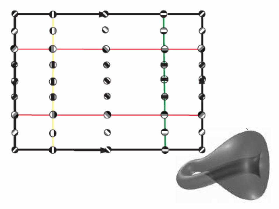
Ver:ces = Regions of Interest Create Rips complex by growing epsilon balls (i.e. decreasing threshold) where distance between two ver:ces is given by where fi =
measurement at loca:on i

hRp://www.ima.umn.edu/videos/?id=856 hRp://ima.umn.edu/2008-‐2009/ND6.15-‐26.09/ac:vi:es/Carlsson-‐Gunnar/imafive-‐handout4up.pdf

hRp://www.ima.umn.edu/videos/?id=1846 hRp://www.ima.umn.edu/2011-‐2012/W3.26-‐30.12/ac:vi:es/Carlsson-‐Gunnar/imamachinefinal.pdf
Applica:on to Natural Image Sta:s:cs With V. de Silva, T. Ishkanov, A. Zomorodian
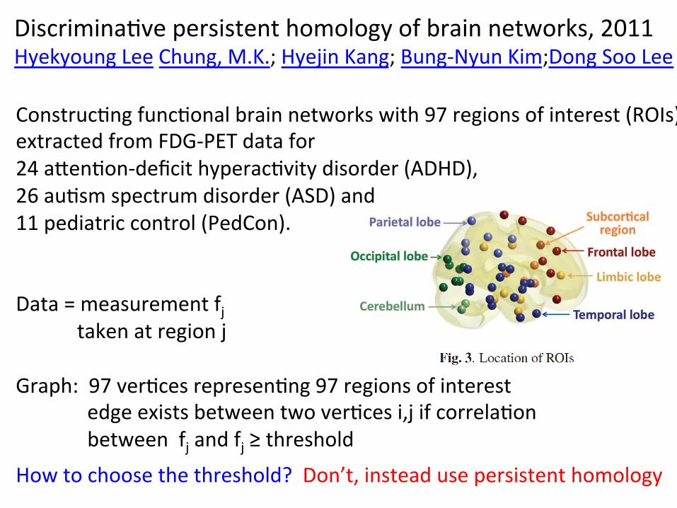
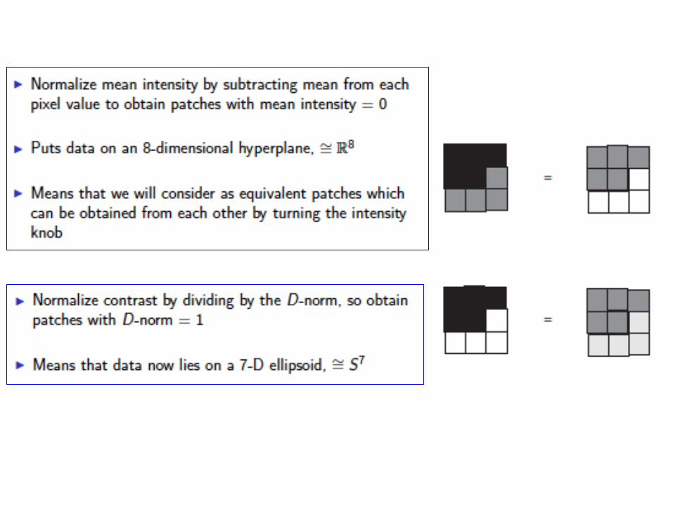
An image taken by black and white digital camera can be viewed as a vector, with one coordinate for each pixel
Each pixel has a “gray scale” value, can be thought of as a real number (in reality, takes one of 255 values) Typical camera uses tens of thousands of pixels, so images lie in a very high dimensional space, call it pixel space, P
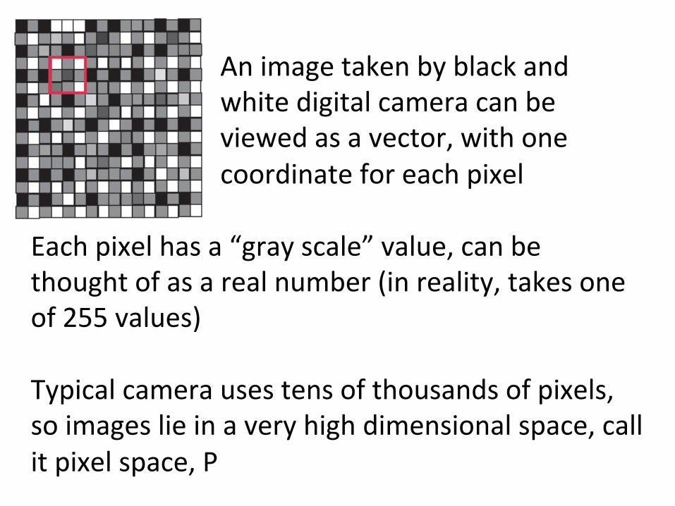
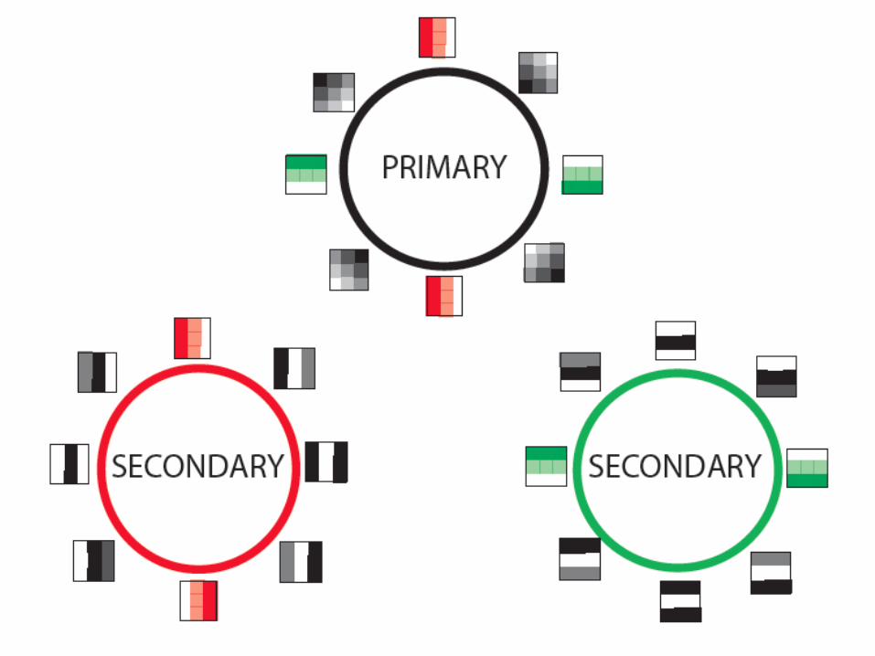
Lee-‐Mumford-‐Pedersen [LMP] study only high contrast patches.
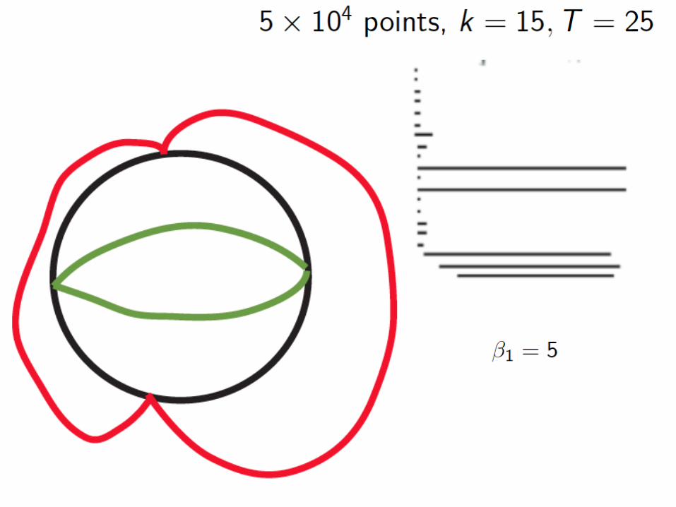
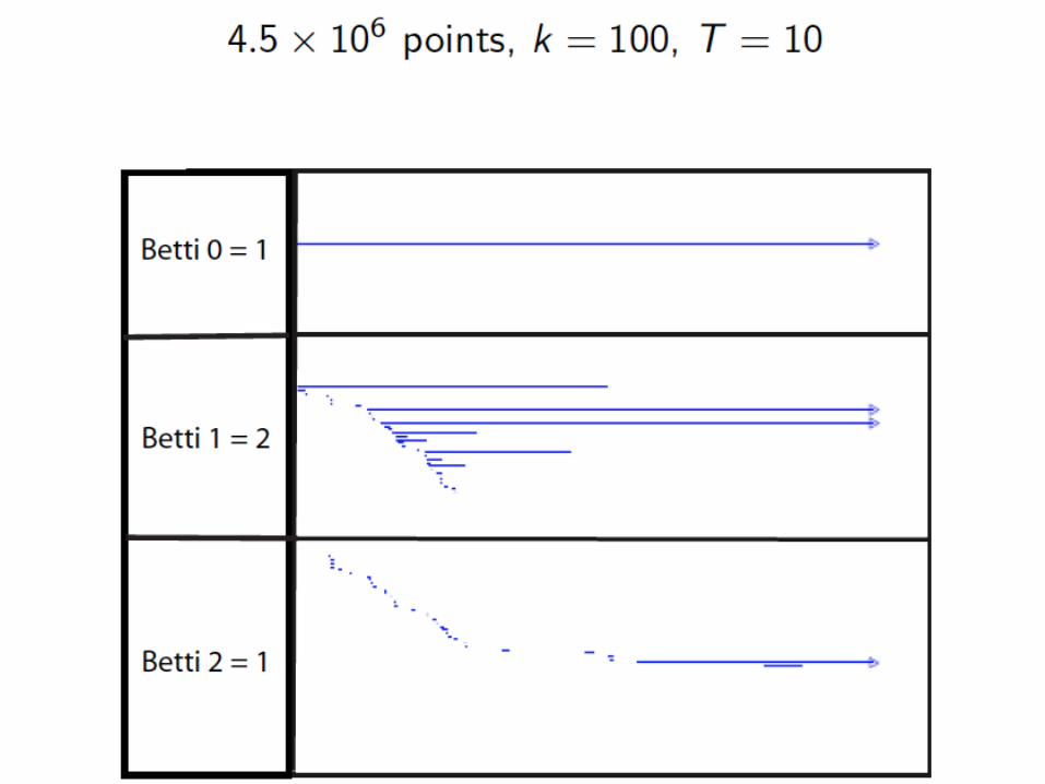
Collec:on: 4.5 x 10⁶ high contrast patches from a collec:on of images obtained by van Hateren and van der Schaaf

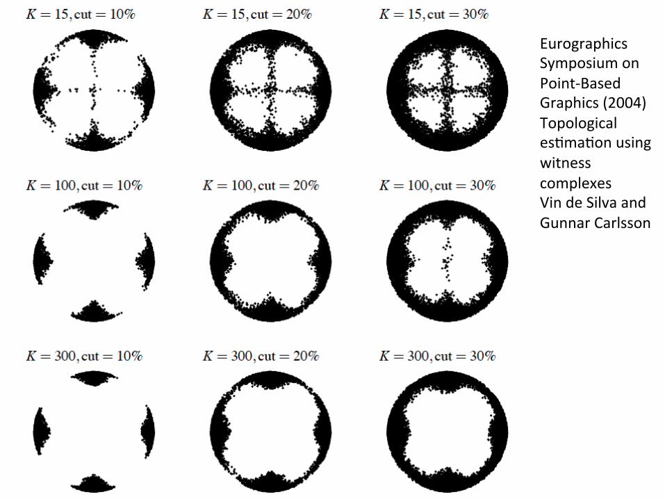
Eurographics Symposium on Point-‐Based Graphics (2004) Topological es:ma:on using witness complexes Vin de Silva and Gunnar Carlsson
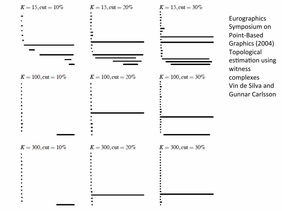
Eurographics Symposium on Point-‐Based Graphics (2004) Topological es:ma:on using witness complexes Vin de Silva and Gunnar Carlsson

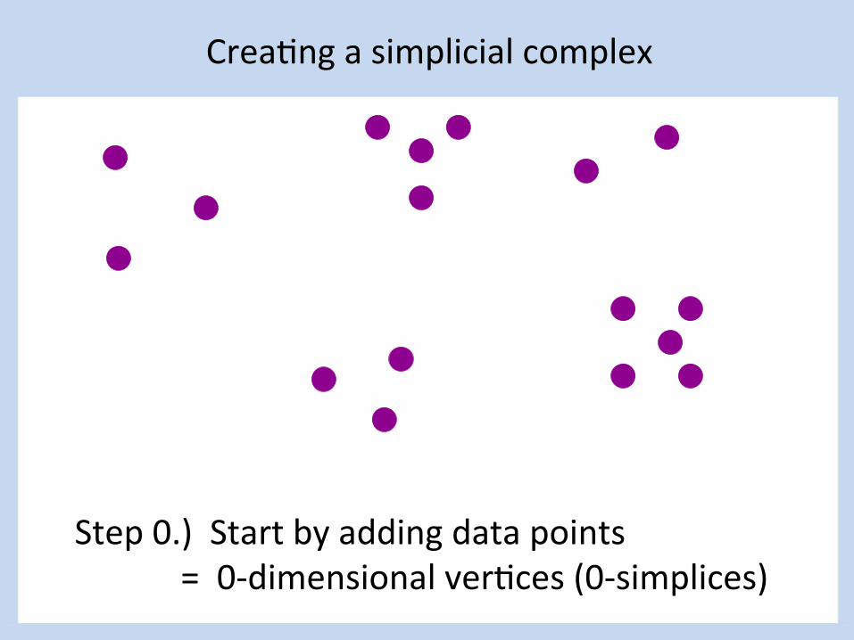
Crea:ng a simplicial complex
Step 0.) Start by adding data points = 0-‐dimensional ver:ces (0-‐simplices)
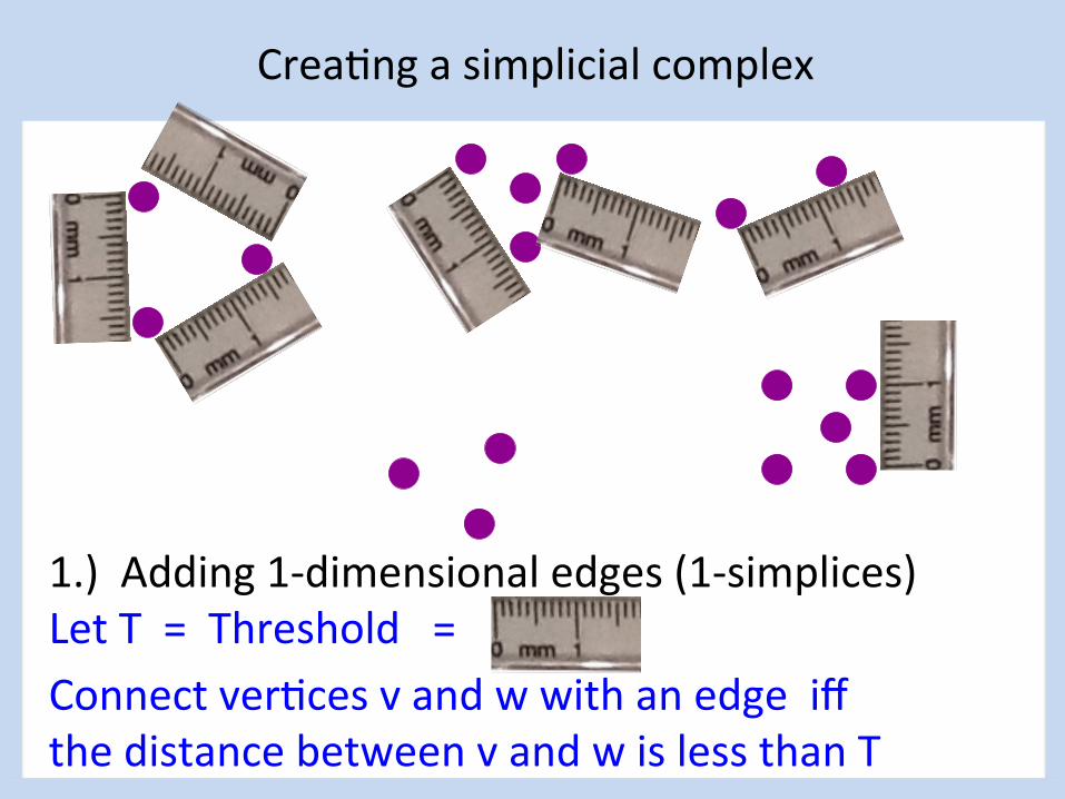
Crea:ng a simplicial complex
1.) Adding 1-‐dimensional edges (1-‐simplices) Let T = Threshold =
Connect ver:ces v and w with an edge iff the distance between v and w is less than T

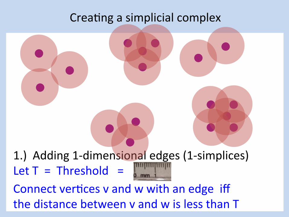
Crea:ng a simplicial complex
1.) Adding 1-‐dimensional edges (1-‐simplices) Let T = Threshold =
Connect ver:ces v and w with an edge iff the distance between v and w is less than T
Crea:ng a simplicial complex
1.) Adding 1-‐dimensional edges (1-‐simplices) Let T = Threshold =
Connect ver:ces v and w with an edge iff the distance between v and w is less than T
Crea:ng a simplicial complex
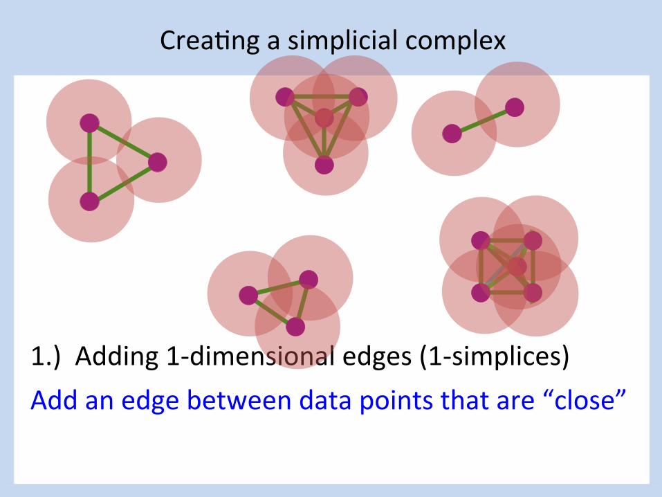
1.) Adding 1-‐dimensional edges (1-‐simplices)
Add an edge between data points that are “close”
Crea:ng a simplicial complex
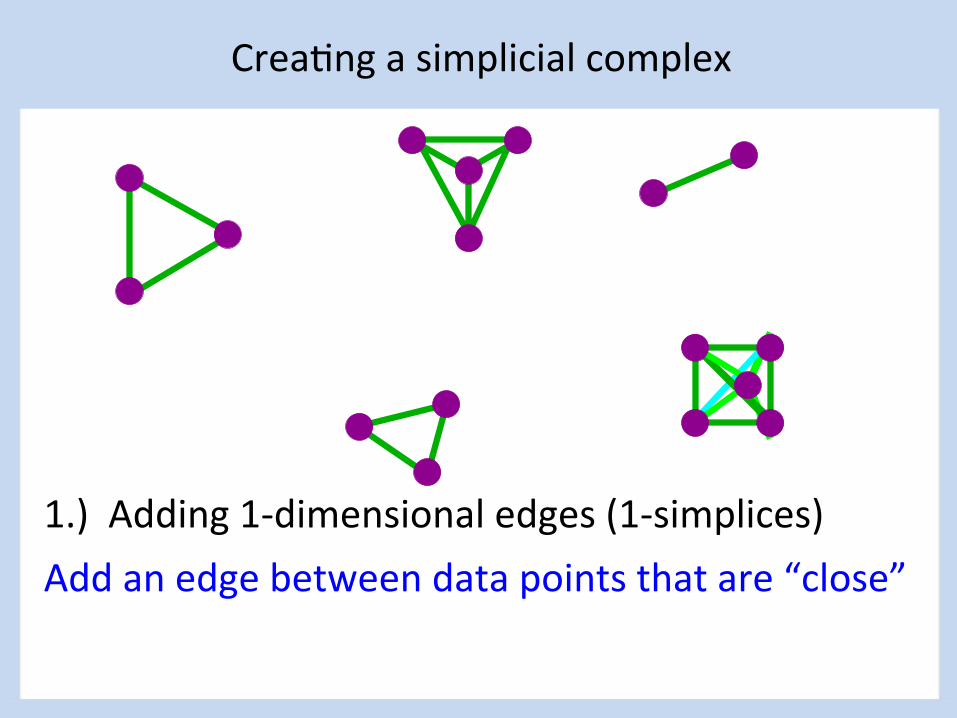
1.) Adding 1-‐dimensional edges (1-‐simplices)
Add an edge between data points that are “close”
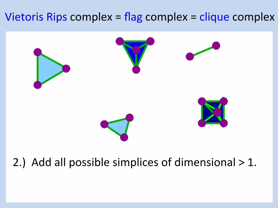
Vietoris Rips complex = flag complex = clique complex
2.) Add all possible simplices of dimensional > 1.
Crea:ng the Čech simplicial complex
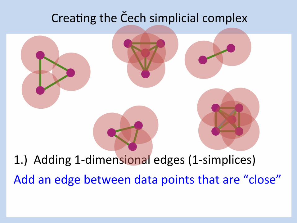
1.) Adding 1-‐dimensional edges (1-‐simplices)
Add an edge between data points that are “close”
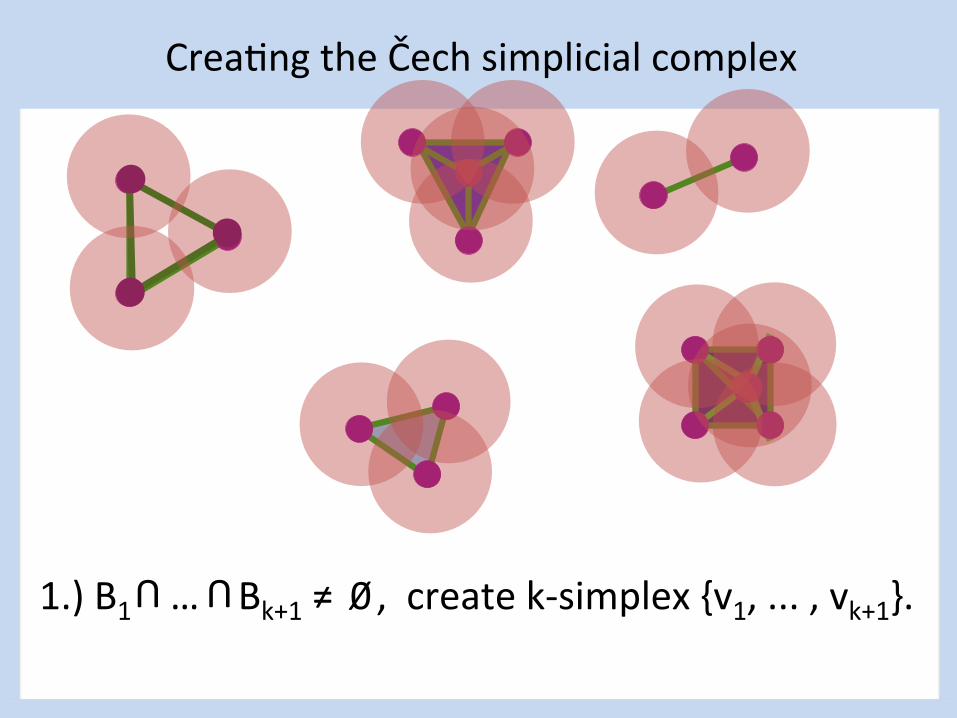
Crea:ng the Čech simplicial complex
1.) B1 … Bk+1 ≠ ⁄ , create k-‐simplex {v1, ... , vk+1}.
U U
0
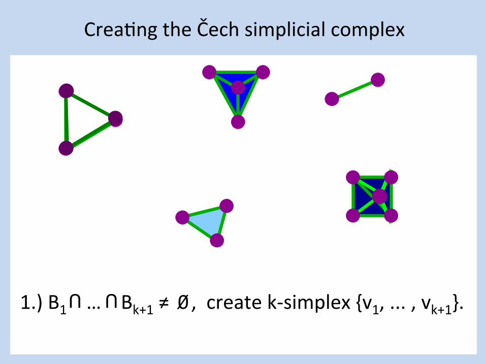
Crea:ng the Čech simplicial complex
1.) B1 … Bk+1 ≠ ⁄ , create k-‐simplex {v1, ... , vk+1}.
U U
0
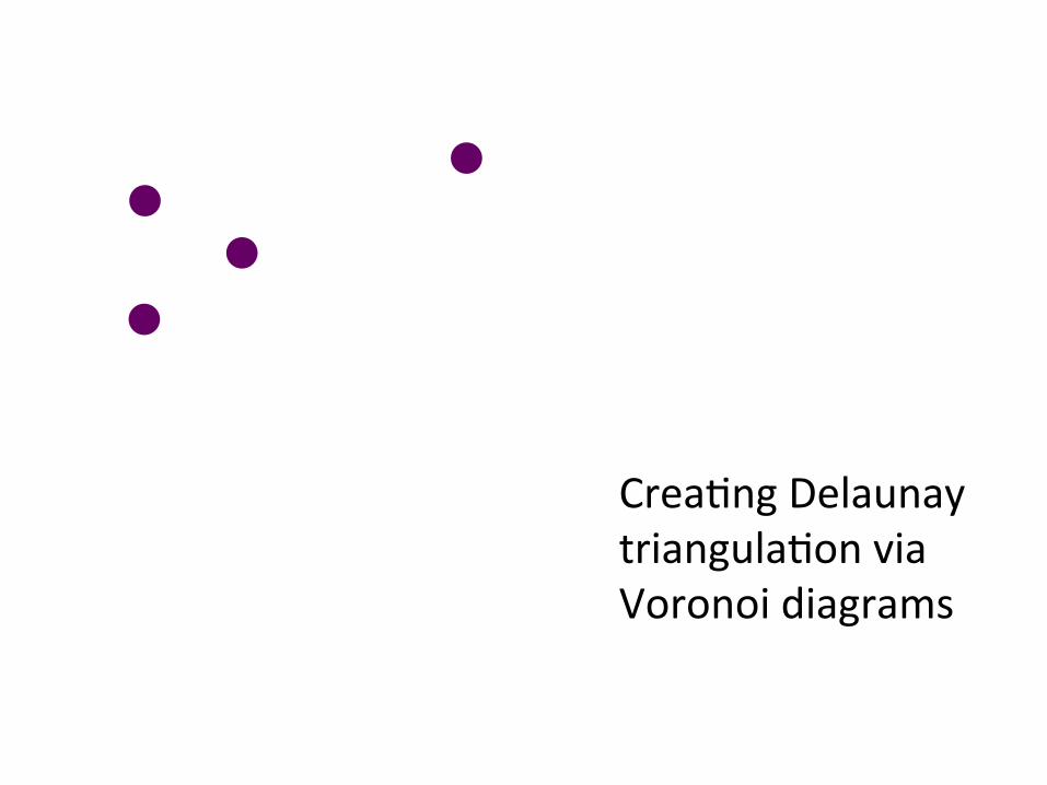
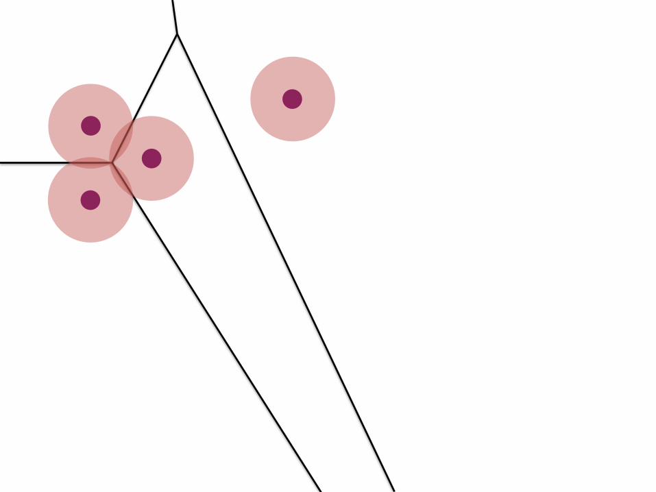
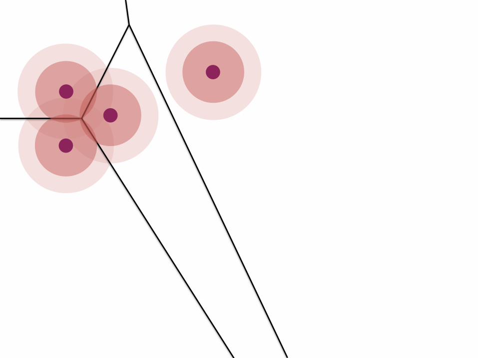
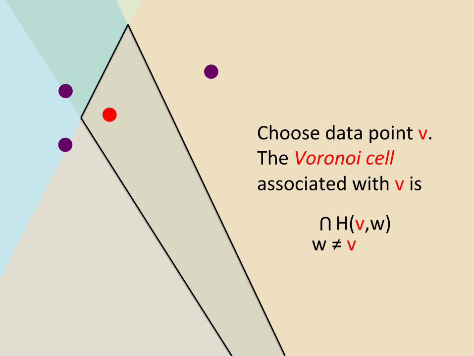
Crea:ng Delaunay triangula:on via Voronoi diagrams
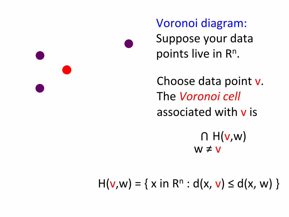
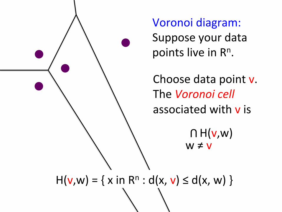
Voronoi diagram: Suppose your data points live in Rn. Choose data point v. The Voronoi cell associated with v is
H(v,w)
U
w ≠ v
H(v,w) = { x in Rn : d(x, v) ≤ d(x, w) }

Voronoi diagram: Suppose your data points live in Rn. Choose data point v. The Voronoi cell associated with v is
H(v,w)
U
w ≠ v
H(v,w) = { x in Rn : d(x, v) ≤ d(x, w) }
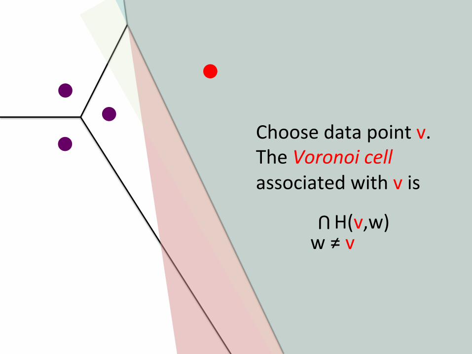
Choose data point v. The Voronoi cell associated with v is
H(v,w)
U
w ≠ v

Choose data point v. The Voronoi cell associated with v is
H(v,w)
U
w ≠ v

Choose data point v. The Voronoi cell associated with v is
H(v,w)
U
w ≠ v
Choose data point v. The Voronoi cell associated with v is
H(v,w)
U
w ≠ v
Voronoi diagram: Suppose your data points live in Rn. Choose data point v. The Voronoi cell associated with v is
H(v,w)
U
w ≠ v
H(v,w) = { x in Rn : d(x, v) ≤ d(x, w) }
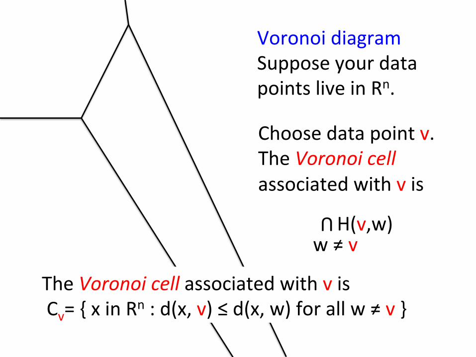
Voronoi diagram Suppose your data points live in Rn.
The Voronoi cell associated with v is Cv= { x in Rn : d(x, v) ≤ d(x, w) for all w ≠ v }
Choose data point v. The Voronoi cell associated with v is
H(v,w)
U
w ≠ v

The Voronoi cell associated with v is Cv= { x in Rn : d(x, v) ≤ d(x, w) for all w ≠ v }
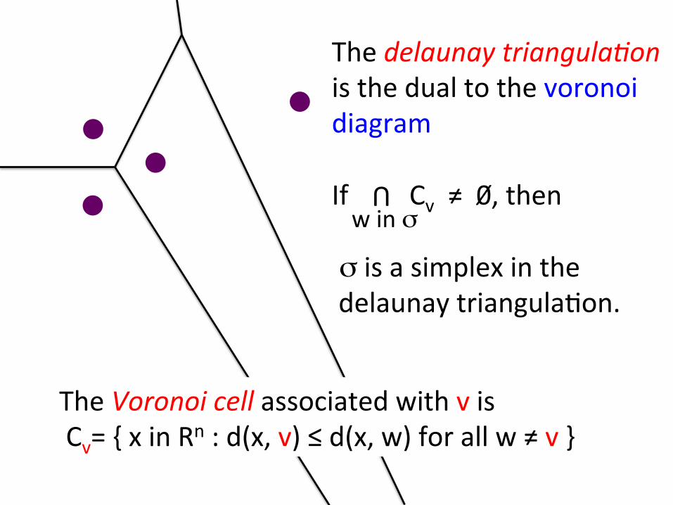
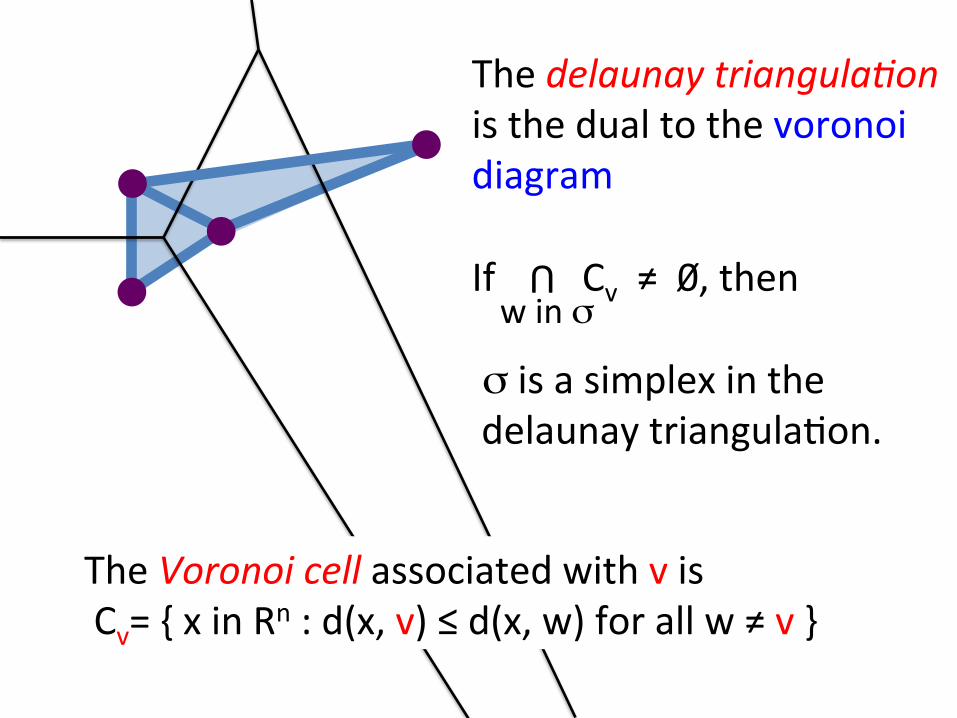
The delaunay triangula0on is the dual to the voronoi diagram If Cv ≠ 0, then σ is a simplex in the delaunay triangula:on.
U
w in σ ⁄
The delaunay triangula0on is the dual to the voronoi diagram If Cv ≠ 0, then σ is a simplex in the delaunay triangula:on.
U
w in σ ⁄
The Voronoi cell associated with v is Cv= { x in Rn : d(x, v) ≤ d(x, w) for all w ≠ v }

The delaunay triangula0on is the dual to the voronoi diagram If Cv ≠ 0, then σ is a simplex in the delaunay triangula:on.
U
w in σ ⁄
The Voronoi cell associated with v is Cv= { x in Rn : d(x, v) ≤ d(x, w) for all w ≠ v }
The delaunay triangula0on is the dual to the voronoi diagram If Cv ≠ 0, then σ is a simplex in the delaunay triangula:on.
U
w in σ ⁄
The Voronoi cell associated with v is Cv= { x in Rn : d(x, v) ≤ d(x, w) for all w ≠ v }