J. Austral. Math. Soc. (Series B) 23 (1982), 332-347

NUMERICAL INTEGRATION ON THE SPHERE

KENDALL ATKINSON

(Received 28 October 1980)

(Revised 1 February 1981)

Abstract

This is a discussion of some numerical integration methods for surface integrals over theunit sphere in R3. Product Gaussian quadrature and finite-element type methods areconsidered. The paper concludes with a discussion of the evaluation of singular doublelayer integrals arising in potential theory.

1. IntroductionThis is a discussion of some numerical integration methods for the surfaceintegral

/ ( / ) = / AQ)do, (1.1)Ju

with U the unit sphere in R3. The integration formulae will include productGaussian quadrature and some methods based on breaking U into smallertriangular elements with various associated low order integration schemes.

The motivation for discussing such methods arises from the desire to solveintegral equations defined over simple smooth surfaces S in R3,

Xp(P) - f K{P, Q)p(Q) da(Q) = +(P), P e S. (1.2)

Such equations can arise in a variety of applications, although we are particu-larly interested in those equations arising from solving potential theory problemsin R3. To deal with integrals over a general surface S, we assume there is asmooth 1-1 mapping of U onto S; then an integral over S can be transformedinto one of the form (1.1).

© Copyright Australian Mathematical Society 1982.

332

[2 ] Numerical integration on the sphere 333

The product Gaussian quadrature formula is discussed and illustrated inSection 2. Methods for triangulating the sphere and some associated integrationformulas are given in Section 3. Since most kernel functions K(P, Q), in (1.2),are singular in potential theory applications, we discuss the evaluation of onesuch integral in Section 4.

For a review of integration methods on the sphere, see Keast and Diaz [6],Lebedev [7], and Stroud [13, Sections 2.6 and 8.4]. The methods discussed in thepresent paper are not optimal, but they are well-suited to the solution of integralequations. Moreover, the theory of optimal methods is far from complete, as hasbeen noted in [7]; consequently it would not be possible to carry out a completeerror analysis of the resulting numerical methods for solving (1.2).

2. Product Gaussian quadrature

Let / ( / ) be written using spherical coordinates

/ ( / ) = F' fW F{9, <j>) sin 0 dB d<f>, (2.1)•'o •'o

with/(0, <J>) =f(x, y, z). The integral is approximated by1m m

4(/) = ^ 2 2 " , M , <*>,)• (2.2)

The {0,} are chosen so that (cos(0,)} and {tv,} are the Gauss-Legendre nodesand weights on [-1, 1]. The points ty are evenly spaced on [0, 2m\ with spacing•n/m; usually

<t>j=jv/m or \j - ^ U/m. (2.3)

With this choice of node points and weights, Im{f) integrates exactly anypolynomial f(x, y, z) of degree less than 2m; see [13, page 40] for a proof. For anintegration formula, the degree of precision is n if the formula is exact for somepolynomial of degree n + 1. Hence Im(f) has degree of precision 2m — 1.

The formula Im(f) is less efficient than the optimal formulae of [7], but notbadly so. For methods of an increasing degree of precision, Lebedev introducesthe efficiency index

) , (2.4)

where n is the degree of precision and N(n) the number of associated nodepoints on if. The larger the index for a given n, the more efficient is the method.The formulae developed by Lebedev satisfy ij(n) -» 1 as n -» oo. The aboveGaussian formula has index ij(2m — 1) = 2/3 for m > 1. Lebedev's formulaeuse only 2/3 the number of node points used by Im(f). This is not a largedifference and it is offset somewhat by the ease with which Im(f) is constructed.

334 Kendall Atkinson [3]

Convergence results for Im(f) can be obtained from an approximation theo-rem of Ragozin [11]. Using this, it is straightforward to show that, if f(x,y, z) isk times continuously differentiable on U, then

|/(/) - Uf)\ < Cl ((2m - l)k) for m > 1. (2.5)

This bound shows the same rapid convergence associated with Gaussian quadra-ture for one variable integration. A short proof of (2.5) is given in [1].

EXAMPLES. Four numerical examples will be given, and they will be referencedby the four different surfaces 5, that are used. The first two examples are

f ex da, i = 1, 2, (2.6)

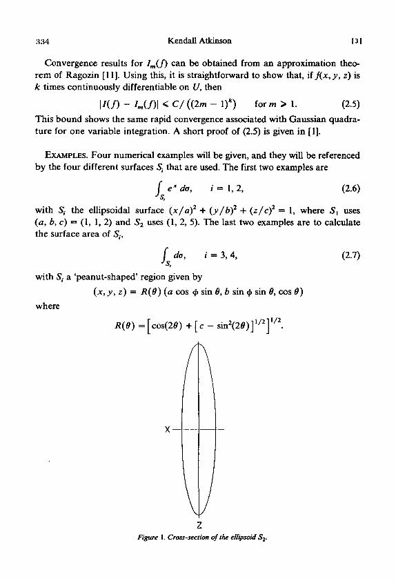
with S, the ellipsoidal surface (x/a)2 + (y/b)2 + (z/cf = 1, where 5, uses(a, b, c) = (1, 1, 2) and S2 uses (1, 2, 5). The last two examples are to calculatethe surface area of 5,,

f da,Js,i = 3, 4, (2.7)

with S, a 'peanut-shaped' region given by

(x,y, z) = R(6) (a cos <j> sin 9, b sin <f> sin 9, cos 9)

where

R(9) =[cos(20) +[c - sin2(20)]1/2]'/2.

Figure 1. Cross-section of the ellipsoid S2-

[4 ] Numerical integration on the sphere 335

Figure 2. Cross-section of the surface S3.

Figure 3. Cross-section of the surface St.

Surface 53 uses (a, b, c) = (1, 2, 2) and S4 uses (1, 2, 1.1). The cross-sections inthe x, z-plane of the surfaces S2, S3, and 54 are shown in Figures 1 to 3. Surfaces5"2 and S4 are somewhat more ill-behaved than 5, and S3.

Table 1 contains the numerical results for the four integrals. The column ngives the number of integration nodes. As expected, the convergence is rapid.

336 Kendall Atkinson

TABLE 1

Errors for product Gaussian quadrature

[ s ]

m n

4 328 128

12 28816 51220 800

Relative error for the integration over 5,

i = 1

-3.0E-4-1.3E-6-9.0E-9

O.0E-12<5.0E-12

/ = 2

-1.5E-3-8.6F-5-7.3E-6-7.9E-7-9.9E-8

i - 3

7.8E-31.4E-4

-3.3E-6-3.7E-7-1.2E-8

-3.4E-2-2.2E-2-5.9E-3-1.4E-3-3.7E-4

3. Finite element integration

Letting {A,, . . . , An} be a triangulation of U, we can write

/(/)=£ JAAQ)da. (3.1)

We will consider numerical approximations to / ( / ) based on approximatingeach integral over Ay using a fixed low order integration rule. First, we discusshow to triangulate U.

The usual manner of subdividing U is based on using a rectangular ortriangular grid on the rectangle {(0, <£)|0 < 9 < 7r, 0 < <|> < 2IT), and this ismapped onto a triangulation of U using the standard spherical coordinatesformula. The advantage of this method is its simplicity, and usually it is rapid toimplement. The main disadvantage is that it results in a very nonuniformdistribution of nodes and elements on U; usually there are relatively more nodesnear the poles z = ± 1. The elements are also quite varied in shape and size, ingeneral. For these reasons, we consider another method of subdivision.

Create an initial triangulation of U by inscribing a tetrahedron, octahedron,or icosahedron inside U, and then project it outward onto the surface U. Thisgives a uniform subdivision of equilateral spherical triangles, with 4, 8, or 20faces, respectively. To subdivide an existing triangulation {A,}, we divide eachface A, into four smaller triangles: find the midpoints of the sides of A,, and thenconnect them by great circle paths. If A,- is not too large, then the four newtriangles created from A, will be almost congruent, and will be nearly similar toA,. This triangulation method leads to a fairly uniform subdivision of U,particularly when the initial subdivision is an icosahedron. Denote the threetriangulation schemes by T,n, Ton, and Tin, depending on whether the initial

[6] Numerical integration on the sphere 337

triangulation uses a tetrahedron, octahedron, or icosahedron, The subscript nindicates the number of faces.

THE CENTROID RULE. The simplest method for estimating the integral over A,is

(3.2)

where Qt is the centroid of A,. If t>,, v2 and u3 denote the vertices of A,, define

' Qi = («i + v2 + v3)/\vi + v2+ v3\. (3.3)

Using this in (3.1), we obtain

/(/) « £ /(ft) Area(A,) = Cn(f), (3.4)

and we shall call this the 'centroid rule'. This simple rule is surprisingly accurate,especially when certain triangulations of U are being used.

If/((?) is twice continuously differentiate on U, then a bound on the rate ofconvergence is given by

A proof is sketched later in this section. The numerical results given belowalso seem to confirm the correctness of the order.

Nonetheless, the method has another interesting aspect. Table 2 gives thedegree of precision d of Cn(f) for the various polyhedral triangulation schemes.These are somewhat surprising results for such a simple method. Clearly, thistriangulation method is important, as other nonuniform triangulations generallyhave only degree of precision 0 or 1. The results of Table 2 can be proved in astraightforward way, based on the results of [12].

TABLE 2

Degree of precision of the centroid rule

Triangulation

Degree of Precision

T T T1 l,n A o,n * i,n

2 3 5

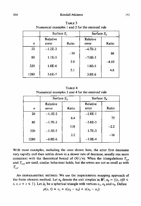
EXAMPLES. We use the integrals (2.6) and (2.7) that were used for the productGaussian quadrature. The triangulation method is Tin, and the results are givenin Tables 3 and 4.

338 Kendall Atkinson

TABLE 3

Numerical examples 1 and 2 for the centroid rule

[71

n

80

320

1280

Surface S1,

Relativeerror

— 1.Z.E.-J

1.1E-5

1.8E-6

3.6E-7

Ratio

-10

5.9

5.1

Surface S2

Relativeerror

—4.7E-3

-7.0E-5

1.8E-5

3.8E-6

Ratio

66

-4.10

4.6

TABLE 4

Numerical examples 3 and 4 for the centroid rule

n

20

80

320

1280

Surface S3

Relativeerror

-1.1E-2

-1.7E-3

-1.5E-5

-6.8E-6

Ratio

6.4

118

2.2

Surface SA

Relativeerror

-2.8E-1

-3.8E-3

1.7E-3

-1.0E-4

Ratio

75

-2.2

-16

With most examples, including the ones shown here, the error first decreasesvery rapidly and then settles down to a slower rate of decrease, usually one moreconsistent with the theoretical bound of O(\/n). When the triangulations Ttn

and To „ are used, similar behaviour holds, but the errors are not as small as with

A N ISOPARAMETRIC METHOD. We use the isoparametric mapping approach ofthe finite element method. Let a0 denote the unit simplex in R2, a0 = {(s, t)\0 <s, t, s + t < 1}. Let A, be a spherical triangle with vertices vu v2 and v3. Define

p(s, t) = o, + t(v2 - u,) + s(v3 - c,)

(8) Numerical integration on the sphere 339

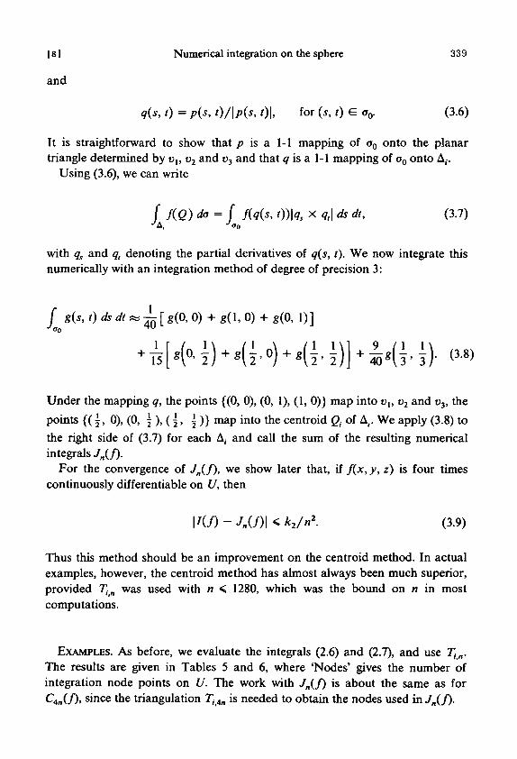
and

q(s, t) = p(s, t)/\p(s, 01, for (s, t) G a0. (3.6)

It is straightforward to show that p is a 1-1 mapping of 0O onto the planartriangle determined by vu v2 and v3 and that q is a 1-1 mapping of a0 onto A,.

Using (3.6), we can write

f(Q) do = \ f{q{s, t))\qs X q,\ ds dt, (3.7)J

with qs and q, denoting the partial derivatives of q(s, t). We now integrate thisnumerically with an integration method of degree of precision 3:

g(s, t)dsdt^~[ g(0, 0) + g(l, 0) + g(0, 1)]'0 W

+ T^

Under the mapping q, the points {(0, 0), (0, 1), (1, 0)} map into vx, v2 and v3, thepoints {(j, 0), (0, \ ), ( j , j )} map into the centroid Qt of A,. We apply (3.8) tothe right side of (3.7) for each A, and call the sum of the resulting numericalintegrals Jn(f).

For the convergence of /„(/), we show later that, if f(x, y, z) is four timescontinuously differentiable on U, then

|/(/) - JnU)\ < k2/n\ (3.9)

Thus this method should be an improvement on the centroid method. In actualexamples, however, the centroid method has almost always been much superior,provided Tin was used with n < 1280, which was the bound on n in mostcomputations.

EXAMPLES. AS before, we evaluate the integrals (2.6) and (2.7), and use Tin.The results are given in Tables 5 and 6, where 'Nodes' gives the number ofintegration node points on U. The work with •/„(/) is about the same as forQn(/)>

s m c e t n e triangulation 7],M is needed to obtain the nodes used in Jn(f).

340 Kendall Atkinson

TABLE 5

Numerical examples 1 and 2 for the isoparametric method

[9]

n Nodes

20 62

80 242

320 962

Surface S,

Relativeerror

-2.8E-2

-2.OE-3

-1.3E-4

Ratio

13.7

15.3

Surface S2

Relativeerror

-3.0E-2

-2.1E-3

-1.3E-4

Ratio

14.3

16.0

TABLE 6

Numerical examples 3 and 4 for the isoparametric method

n Nodes

20 62

80 242

320 962

Surface S3

Relativeerror

-3.2E-2

-2.9E-3

-1.3E-4

Ratio

11

12

Surface S4

Relativeerror

-1.8E-1

-5.8E-3

8.4E-4

Ratio

31

-6.9

Based on our examples, the centroid rule should be used in preference to theisoparametric method /„(/), provided n is not too large and Tin is used. Withother values of n or other triangulations, /„(/) is much more competitive, andpossibly superior. Comparing with the other examples for the product Gaussianquadrature, the latter is generally superior in accuracy to Cn(/), especially atmoderate to high error tolerances.

ERROR BOUND DERIVATIONS. We will give only a sketch of the proof of (3.9);the details are straightforward, but algebraically complicated. First, note that theintegration rule (3.8) is exact for all polynomials g(s, I) of degree < 3. For ageneral differentiable function g(s, t), an error formula can be found in thestandard way: expand g(s, t) in a Taylor series through the third degree plus aremainder term, and apply the error functional for (3.8) to this equation. Theerror will be proportional to the fourth derivatives of g.

I io 1 Numerical integration on the sphere 341

To apply this to deriving (3.9), first assume that f(x,y, z) is defined in aneighborhood of U, with continuous and bounded fourth order derivatives.Since (3.8) is applied to (3.7), consider the fourth derivative of the integrand in(3.7). It can be shown that

34

, t))\q, X q,\] <Cmax{|t;1-t;2|6, |t>, - t>3|6}. (3.10)

In addition, the following results can be shown for our triangulations Tt „, To „,and Tun:

cjn < Area(A,) < c2/2, for i = 1, . . . , n, (3.12)

where c, and c2 > 0 and independent of n; furthermore,

c3 max{|c, - v2f, \v2 - v3\2, \v3 - t>,|2} < Area(A,)

< c4 min{|t>i - v2\2, \v2 - v3\

2,\v3 - u, |2}, (3.12)

with i = 1, . . . , n, u,, v2 and v3 the vertices of A,, and c3 and c4 > 0 indepen-dent of n. Combining all of these results with the error formula for (3.8), derivedusing a Taylor series, we obtain (3.9).

For functions f(Q) defined only on U, if they are four times differentiateusing a local parametrization on U, then they can be extended to a new functionon a neighborhood of U; and the extensions can be chosen to have the samedegree of differentiability. For a discussion of this, see [4, pages 13, 100].

The proof of (3.5) is quite similar. We write

>-/(&)Area(A,)

M*. 0)1* x q,\ as * - \j[q{\, I))|,,(I, I) x q,{\, I

2

= £/'> + E?>. (3.13)

The point ( \ , 3 ) is the centroid of o0, and Q, = q{ y , 3 ). The integration rule

/ g{s,t)dsdt~)rg(\,\) (3.14)

has degree of precision 1. Using the same kind of proof as that given for (3.9), itfollows that

P = O(l/n2). (3.15)

342 Kendall Atkinson [ 111

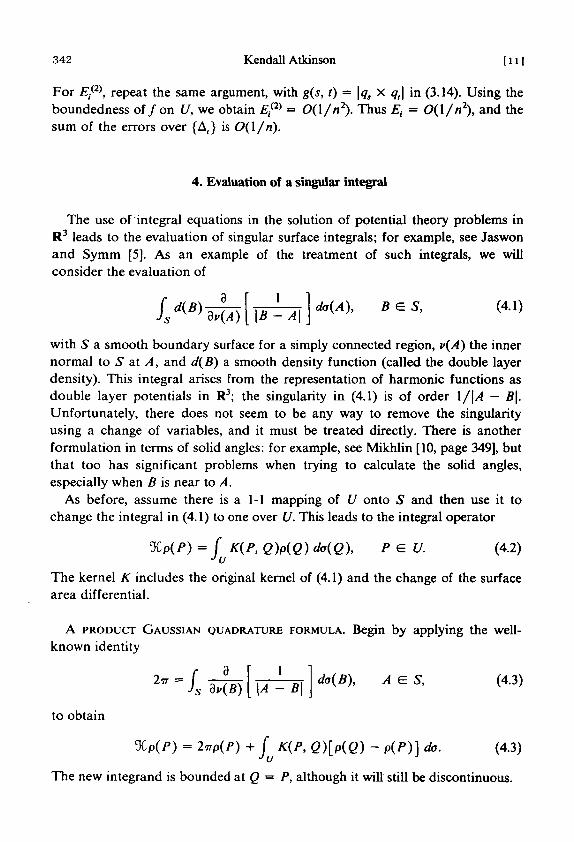
For ZT/2), repeat the same argument, with g(s, i) = \qs X q,\ in (3.14). Using theboundedness o f /on U, we obtain £,(2) = 0(1/n2). Thus Ei = O(l//i2), and thesum of the errors over {A,} is O(\/n).

4. Evaluation of a singular integral

The use of integral equations in the solution of potential theory problems inR3 leads to the evaluation of singular surface integrals; for example, see Jaswonand Symm [5]. As an example of the treatment of such integrals, we willconsider the evaluation of

f d(B)dv(A)

with S a smooth boundary surface for a simply connected region, v(A) the innernormal to S at A, and d(B) a smooth density function (called the double layerdensity). This integral arises from the representation of harmonic functions asdouble layer potentials in R3; the singularity in (4.1) is of order \/\A — B\.Unfortunately, there does not seem to be any way to remove the singularityusing a change of variables, and it must be treated directly. There is anotherformulation in terms of solid angles: for example, see Mikhlin [10, page 349], butthat too has significant problems when trying to calculate the solid angles,especially when B is near to A.

As before, assume there is a 1-1 mapping of U onto S and then use it tochange the integral in (4.1) to one over U. This leads to the integral operator

%p(P) = f K(P, Q)p(Q) da(Q), P&U. (4.2)Ju

The kernel K includes the original kernel of (4.1) and the change of the surfacearea differential.

A PRODUCT GAUSSIAN QUADRATURE FORMULA. Begin by applying the well-known identity

to obtain

%p(P) = 2-np(P) + f K(P, Q)[P(Q) - p(P)] da. (4.3)

The new integrand is bounded at Q = P, although it will still be discontinuous.

Numerical integration on the sphere 343

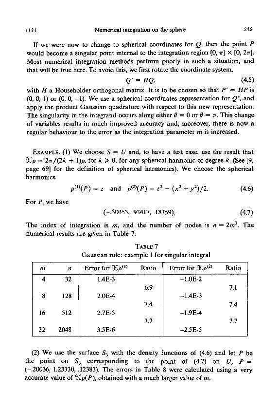
If we were now to change to spherical coordinates for Q, then the point Pwould become a singular point internal to the integration region [0, w] X [0, 2m\.Most numerical integration methods perform poorly in such a situation, andthat will be true here. To avoid this, we first rotate the coordinate system,

Q' = HQ, (4.5)

with H a Householder orthogonal matrix. It is to be chosen so that P' = HP is(0, 0, 1) or (0, 0, -1). We use a spherical coordinates representation for Q', andapply the product Gaussian quadrature with respect to this new representation.The singularity in the integrand occurs along either 0 = 0 or 9 = n. This changeof variables results in much improved accuracy and, moreover, there is now aregular behaviour to the error as the integration parameter m is increased.

EXAMPLE. (1) We choose S = U and, to have a test case, use the result that%p = 2ir/(2k + l)p, for k > 0, for any spherical harmonic of degree k. (See [9,page 69] for the definition of spherical harmonics). We choose the sphericalharmonics

pm(P) = z and p(2>(P) = z2 - (x2 + y2)/2. (4.6)

For P, we have

(-.30353, .93417, .18759). (4.7)

The index of integration is m, and the number of nodes is n = 2m2. Thenumerical results are given in Table 7.

TABLE 7

Gaussian rule: example 1 for singular integral

m

4

8

16

32

n

32

128

512

2048

Error for %pw

1.4E-3

2.0E-4

2.7E-5

3.5E-6

Ratio

6.9

7.4

7.7

Error for SCp(2)

-1.0E-2

-1.4E-3

-1.9E-4

-2.5E-5

Ratio

7.1

7.4

7.7

(2) We use the surface S3 with the density functions of (4.6) and let P bethe point on 53 corresponding to the point of (4.7) on U, P =(-.20036, 1.23330, .12383). The errors in Table 8 were calculated using a veryaccurate value of %p(P), obtained with a much larger value of m.

344 Kendall Atkinson [13]

TABLE 8

Gaussian rule: example 2 for singular integral

m

4

8

16

32

n

32

128

512

2048

Error for 9Cp(1)

-5.2E-2

-5.7E-4

-5.4E-5

-7.2E-6

Ratio

92

11

7.4

Error in DCp<2)

5.6E-2

-6.0E-4

-3.0E-5

-4.0E-6

Ratio

-93

20

7.4

In these examples and with all other examples we calculated, the error has theasymptotic form

c/ (m3) + O{\/m<). (4.8)

As the surface becomes more ill-behaved, the value of m must be larger beforethe behaviour (4.8) becomes apparent. With surfaces S2 and S4, this happenswith m = 64, but the error is still quite small with smaller values of m. With anerror of the form (4.8), Richardson extrapolation can be used to accelerate theconvergence, and that should be an important tool with these singular problems.A similar strategy is suggested by Lyness [8].

A FINITE ELEMENT INTEGRATION FORMULA. Most numerical methods forevaluating (4.1) are based on first writing it as a sum of smaller integrals, basedon some triangulation of S,

£ / d{B)-= 1 "'A,

1dv(B) [\A-B\

da(B).

Usually each integral over A, is approximated by the central rule, and thesurface area of A, is approximated by the area of the planar triangle determinedby the vertices of Ay. For examples, see Jaswon and Symm [5, page 233], Birtleset al. [3], and Wait [14, page 303]; the last paper also uses a quadraticisoparametric method, with improved results. This is a very flexible approach tothe evaluation of integrals like (4.1), but it also leads to greater inaccuracy thanif the special nature of the kernel and surface were taken into account.

We approximate (4.2) using the centroid rule, with a crude modification toavoid elements containing the singular point P, using

[ 141 Numerical integration on the sphere 345

, QJMQJ) Area(A,)

\ * - 2 K(P, Qj) Aica^j)]P(V), (4.9)L ^ A , J

where Qj is the centroid of A,, and V is some centrally located point in the unionof all elements Ay containing P. The approximation uses (4.3). Empirically, thebehaviour of this method is best when P is a centroid of one of the triangles A,.

EXAMPLE. (1) We let S = U, and let p and P be given by (4.6) and (4.7). Thetriangulation Tin is used, and P is a centroid of one of the faces of Ti20- Theresults are given in Table 9.

TABLE 9

Centroid rule: example 1 for singular integral

n

20

80

320

1280

5120

Error in %pm

-5.7E-3

-9.4E-4

-1.4E-4

-1.9E-5

-2.9E-6

Ratio

6.1

7.0

7.1

6.7

Error in DCp(2>

4.2E-2

6.8E-e

9.8E-4

1.4E-4

2.1E-5

Ratio

6.2

7.0

7.1

6.6

(2) We use the same surface S3, density p, and point P as with example 2 forproduct Gaussian quadrature. The results are given in Table 10.

TABLE 10

Centroid rule: example 2 for singular integral

n

20

80

320

1280

5120

Error in %pw

1.6E-1

-5.9E-2

1.6E-2

-4.1E-3

1.0E-3

Ratio

-2.7

-3.7

-3.8

-4.0

Error in 9Cp(2)

1.2

-1.4E-2

3.5E-3

-1.3E-4

1.9E-4

Ratio

-83

-4.0

-28

-.7

346 Kendall Atkinson [ i s |

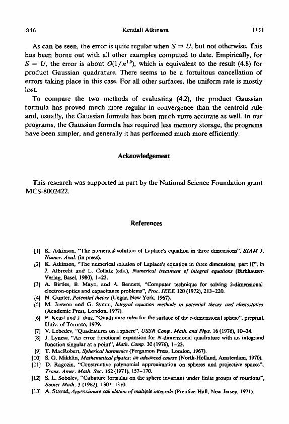
As can be seen, the error is quite regular when S = U, but not otherwise. Thishas been borne out with all other examples computed to date. Empirically, forS = U, the error is about O(l/n15), which is equivalent to the result (4.8) forproduct Gaussian quadrature. There seems to be a fortuitous cancellation oferrors taking place in this case. For all other surfaces, the uniform rate is mostlylost.

To compare the two methods of evaluating (4.2), the product Gaussianformula has proved much more regular in convergence than the centroid ruleand, usually, the Gaussian formula has been much more accurate as well. In ourprograms, the Gaussian formula has required less memory storage, the programshave been simpler, and generally it has performed much more efficiently.

Acknowledgement

This research was supported in part by the National Science Foundation grantMCS-8002422.

References

[1] K. Atkinson, "The numerical solution of Laplace's equation in three dimensions", SI AM J.Numer. Anal, (in press).

[2] K. Atkinson, "The numerical solution of Laplace's equation in three dimensions, part II", inJ. Albrecht and L. Collate (eds.), Numerical treatment of integral equations (Birkhauser-Verlag, Basel, 1980), 1-23.

[3] A. Birtles, B. Mayo, and A. Bennett, "Computer technique for solving 3-dimensionalelectron-optics and capacitance problems", Proc. IEEE 120(1972), 213-220.

[4] N. Gunter, Potential theory (Ungar, New York, 1967).[S] M. Jaswon and G. Symm, Integral equation methods in potential theory and elastostatics

(Academic Press, London, 1977).[6] P. Keast and J. diaz, "Quadrature rules for the surface of the ̂ -dimensional sphere", preprint,

Univ. of Toronto, 1979.[7] V. Lebedev, "Quadratures on a sphere", USSR Comp. Math, and Phys. 16 (1976), 10-24.[8] J. Lyness, "An error functional expansion for jV-dimensional quadrature with an integrand

function singular at a point", Math. Comp. 30 (1976), 1-23.[9] T. MacRobert, Spherical harmonics (Pergamon Press, London, 1967).

[10] S. G. Mikhlin, Mathematical physics: an advanced course (North-Holland, Amsterdam, 1970).[11] O. Ragozin, "Constructive polynomial approximation on spheres and projective spaces",

Trans. Amer. Math. Soc. 162 (1971), 157-170.[12] S. L. Sobolev, "Cubature formulas on the sphere invariant under finite groups of rotations",

Soviet Math. 3 (1962), 1307-1310.[13] A. Stroud, Approximate calculation of multiple integrals (Prentice-Hall, New Jersey, 1971).

1161 Numerical integration on the sphere 347

[14] R. Wait, "Use of finite elements in multi-dimensional problems in practice", in J. Walsh andM. Delves (eds.), Numerical solution of integral equations (Oxford University Press, 1974),300-311.

Mathematics DepartmentUniversity of IowaIowa CityIowa 52242U.S.A.