Embed Size (px)
Citation preview

Sequential Resource Allocation for Nonprofit Operations
Robert W. Lien, Seyed M.R. Iravani and Karen R. Smilowitz
Department of Industrial Engineering and Management SciencesNorthwestern University, Evanston, IL 60208, USA
Abstract
This paper studies a sequential resource allocation problem motivated by distribution opera-tions of a nonprofit organization. The alternate objectives that arise in nonprofit, as opposed tocommercial, operations lead to new variations on traditional problems in operations research andinventory management. Specifically, we consider the problem of distributing a scarce resource tomeet sequentially observed customer demand. In a commercial setting, the amount distributed toeach customer is determined to maximize profit; however, this objective may lead to inequitabledistributions among customers. Our work in a nonprofit setting solves the sequential resource al-location problem with an objective function aimed at equitable and sustainable service. We defineservice in terms of fill rate (the ratio of the allocated amount to observed demand) and develop anobjective function to maximize the expected minimum fill rate among customers. Through a dy-namic programming framework, we characterize the structure of the optimal allocation policy for agiven sequence of customers. In addition, we address customer visitation sequencing by identifyingproperties to consider in sequencing decisions to optimize the objective. For both inventory allo-cation and customer sequencing decisions, we develop heuristic methods which yield near-optimalsolutions.
Subject classifications: Inventory/production: sequential resource allocation. Transportation.Area of review: Manufacturing, Service and Supply Chain Operations
1 Introduction and Motivation
While America has the strongest national economy with a GDP of 13.2 trillion dollars in 2006, 12.3%
of its population was below the poverty line in that same year. Based on the most recent hunger
study from America’s Second Harvest, thirty-six million Americans suffer from hunger. Twenty-five
million of these Americans rely on America’s Second Harvest and their network of pantries, shelters
and soup kitchens for food. The largest suppliers to these agencies are regional and local food banks.
Food banks are large distribution centers which collect, store and distribute food. Much of this food
is donated by sources of surplus food such as supermarkets and grocery chains. According to the U.S.
Department of Agriculture, 100 billion pounds of food are wasted each year in the United States. The
goal of American’s Second Harvest (ASH) and the agencies in their network is to match surplus food
with those in need. This matching is a large-scale distribution and inventory management problem
that occurs each day at thousands of nonprofit agencies across the country. Much research has been
conducted on related supply chain problems in commercial settings where the goal of such systems
1

is either to maximize profit or minimize cost. Little work, however, has been conducted in nonprofit
applications. In such settings, the objectives are often more difficult to quantify since issues such as
equity and sustainability must be considered, yet efficient operations are still crucial.
Several decades of research in commercial supply chains have resulted in papers that model a wide
range of inventory management decisions. In general, these models are designed to maximize a firm’s
profit and provide useful insight in inventory management. Many firms assign a substantial budget
to R&D activities to improve the profitability of their organization; nonprofit organizations rarely
have funds for such activities. Unfortunately, many models developed for commercial settings are
not applicable to nonprofit organizations. It is essential to provide answers to inventory management
questions that occur in nonprofit organizations such as food banks, where the main objectives are to
ensure that food is distributed fairly and waste is minimized.
The Greater Chicago Food Depository (GCFD) is an active ASH member. According to a 2005
study by the GCFD and ASH, 500,000 people in the Chicago region are served by the GCFD each
year. Lisa Koch, GCFD’s former director of public policy, notes “more and more people are in need
of supplemental and emergency food, and we need continued support to shrink the gap between those
who need help and our means to provide it.” We have worked with the GCFD to address this gap,
focusing on their Food Rescue Program (FRP). The FRP distributes perishable food from donors (e.g.
supermarkets and restaurants) to agencies (e.g. shelters and soup kitchens). Over 80 donors and 100
agencies participate in the FRP, which moves over 4 million pounds of food annually.
The FRP operates 5 truck routes, each visiting, on average, 8 donors and 4-5 agencies daily. A
sample route is shown in Figure 1. Stop A represents the GCFD warehouse where trucks are housed
(referred to as the depot in this paper), stops represented by B through E are donors and stops F
through I are agencies. Due to operating schedules of the donor sites, routes first visit all donors
before visiting agencies. Routes are scheduled weeks in advance and remain fairly regular to facilitate
driver familiarity. The frequency of visits to a location over the course of a month depends on the
supply (for donors) and food need (for agencies).
Donation amounts are unknown until observed upon the driver’s arrival. All donated food is
accepted and loaded; there is typically ample truck capacity for the donated food. Food demand
depends on available storage and budget at the agencies; agencies are charged 4 cents per pound. Under
current operations, because of lack of personnel at agencies and timing of delivery operations, agency
requests are revealed only upon arrival. The allocation of food to agencies is left to the discretion of
2
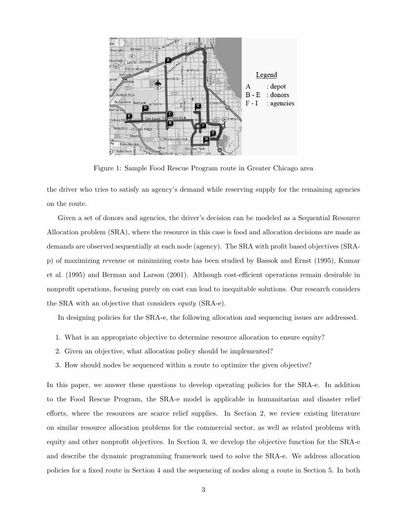
Figure 1: Sample Food Rescue Program route in Greater Chicago area
the driver who tries to satisfy an agency’s demand while reserving supply for the remaining agencies
on the route.
Given a set of donors and agencies, the driver’s decision can be modeled as a Sequential Resource
Allocation problem (SRA), where the resource in this case is food and allocation decisions are made as
demands are observed sequentially at each node (agency). The SRA with profit based objectives (SRA-
p) of maximizing revenue or minimizing costs has been studied by Bassok and Ernst (1995), Kumar
et al. (1995) and Berman and Larson (2001). Although cost-efficient operations remain desirable in
nonprofit operations, focusing purely on cost can lead to inequitable solutions. Our research considers
the SRA with an objective that considers equity (SRA-e).
In designing policies for the SRA-e, the following allocation and sequencing issues are addressed.
1. What is an appropriate objective to determine resource allocation to ensure equity?
2. Given an objective, what allocation policy should be implemented?
3. How should nodes be sequenced within a route to optimize the given objective?
In this paper, we answer these questions to develop operating policies for the SRA-e. In addition
to the Food Rescue Program, the SRA-e model is applicable in humanitarian and disaster relief
efforts, where the resources are scarce relief supplies. In Section 2, we review existing literature
on similar resource allocation problems for the commercial sector, as well as related problems with
equity and other nonprofit objectives. In Section 3, we develop the objective function for the SRA-e
and describe the dynamic programming framework used to solve the SRA-e. We address allocation
policies for a fixed route in Section 4 and the sequencing of nodes along a route in Section 5. In both
3

sections we derive analytical results which provide insights in developing effective heuristic methods.
In Section 6, we combine the heuristic allocation and sequencing methods and compare the results
against optimal operating policies. In Section 7, we present a numerical study to assess the value
of demand information, and in Section 8 we study the expected waste under the optimal allocation
policy. Lastly, in Section 9 we conclude the paper and discuss research extensions.
2 Literature Review
Several papers have addressed allocation for the SRA-p on fixed delivery routes in commercial op-
erations. Bassok and Ernst (1995) examine a system where demand is observed sequentially upon
arrival at a customer. Given varying profit margins by customer, the driver may be willing to trade a
sure profit for potentially higher profit at a customer later in the route. They show that the revenue
maximizing allocation policy at each customer is a threshold policy independent of customer demand.
Kumar et al. (1995) evaluate static and dynamic allocation policies in delivery routes with long travel
times between customers. Static policies are predetermined allocation amounts that do not change
once customers are visited, while dynamic policies adjust as demand is observed. In their model, the
driver has preliminary inventory information for customers, though actual inventory levels change dur-
ing vehicle travel. Berman and Larson (2001) study a similar problem in the allocation of industrial
gases. They apply an incremental cost structure to quantify the value of timely delivery and product
fulfillment. These papers optimize profit/cost-based objectives, where the profit/cost from serving a
customer is directly added in the objective function.
Some research on nonprofit applications have similar additive objective functions that maximize
utility/service or minimize costs, see Chou et al. (2008), Wong and Meyer (1993) and Johnson et al.
(2005). However, the majority of operations research literature in nonprofit settings incorporate equity
as an objective. See Pollock et al. (1994) for a review of operations research work in the public sector,
with a focus on government activities; and Johnson and Smilowitz (2007) for an overview of research
in community-based nonprofit operations. Gass (1994) discusses the differences between private and
public applications of operations research and notes the particular emphasis on equity in nonprofit
operations. Further, Savas (1978) identifies efficiency, effectiveness and equity as key performance
measures in nonprofit settings.
The literature has considered different methods to measure and incorporate equity. In Mandell
(1991), equity is measured with the Gini coefficient, and is incorporated as an objective in a multi-
4

objective mathematical programming model. This work considers the tradeoff between effectiveness
and equity as applied to the allocation of books to libraries. Campbell et al. (2008) explore two
objective functions for the local distribution of supplies in a relief effort. To minimize disparity in
response times to recipients, the authors consider the objectives of minimizing the arrival of supplies to
the last recipient and minimizing the average arrival of supplies. They show that the choice of objective
function can have significant impact on solutions. Swaminathan (2003) considers the application of
allocating scarce drugs to clinics and hospitals. In this work, tradeoffs between equity, effectiveness and
efficiency are modeled in an multi-objective mathematical program. In these papers, static decision
models, such as mathematical programs, are appropriate since decisions are made at a single epoch;
in our work, however, each node represents a decision epoch.
Our paper contributes to the literature by introducing a sequential allocation problem with a
nonprofit objective. By necessity, we employ a measure of equity and an objective function which are
different from what has been done in the literature. Because of the mathematical structure of the
objective function, the solution methods and results from commercial sequential allocation research
are not directly applicable. In this paper, we develop a new model and solution approaches to address
the unique problem motivated by the FRP.
3 Sequential Allocation Model
In Section 3.1, we develop the objective function for the SRA-e. In Section 3.2, we present the dynamic
programming formulation to solve the model with analytical results for optimal values.
3.1 Objective Function Development
Consider the simple FRP example presented in Figure 2, in which the supply is collected from one
donor (source) and distributed to two agencies (nodes). Since all donations are accepted and loaded,
our model aggregates donors into one supply source without loss of generality. The first decision epoch
for the SRA-e model occurs at node 1, which is the first agency visited on the route. Demand (Di) at
node i follows the discrete probability distribution presented in the figure. Let di denote the observed
demand at node i and xi denote the amount allocated to i. We define the fill rate at node i as βi = xidi
.
The amount of initial supply (s0) is a known parameter of the model. Let si denote the units of supply
available upon arrival at node i; therefore, s1 = s0 and si = si−1 − xi−1.
In the example in Figure 2, s0 = 130 units of supply. Upon arrival at node 1, allocation is
5

Figure 2: Example of a food distribution route
determined to optimize a chosen objective function. For example, if the objective is to minimize
expected waste, it is optimal to satisfy all of the observed demand at node 1. Therefore, if d1 = 80,
then x1 = 80, and if d1 = 120, then x1 = 120. As a result, the available supply upon arrival at
node 2 is s2 = 50 with probability 0.5 and s2 = 10 with probability 0.5. The allocation at node 2 is
x2 = min{d2, s2}; the demand at node 2 is fully satisfied if possible. Considering all possible demand
realizations for the nodes, under the objective of minimizing waste, the expected waste is 2.5 units,
which is 2% of the initial supply. The expected fill rates at nodes 1 and 2 are E[β1] = 100% and
E[β2] = 56%, respectively.
The above solution minimizes expected waste (and maximizes expected distribution), yet there is
a 44% difference between the fill rates of the agencies. The goal of maintaining equity among agencies
is not achieved. To consider equity while maintaining a high level of distribution, we consider the
objective of maximizing the expected minimum fill rate (i.e. max{E[min{β1, β2}]
}). Note that the fill
rates of all nodes are bounded below by the minimum fill rate and above by 1. Increasing the minimum
fill rate among all nodes improves overall distribution by increasing the fill rates of all agencies and
improves equity by reducing the difference between fill rates.
We show in Section 3.2 that using dynamic programming under this objective the optimal allocation
policy is as follows: If d1 = 80, then x1 = 75, and if d1 = 120, then x1 = 87. As a result, s2 = 55 with
probability 0.5 and s2 = 43 with probability 0.5. As with the previous objective, x2 = min{d2, s2}.
Considering all four possible demand realizations, the expected fill rates at nodes 1 and 2 are E[β1] =
83% and E[β2] = 91%, respectively. The expected waste is 4.5 units, which is 3.5% of the initial and
only 1.5% more than the previous objective.
We focus on maximizing the expected minimum fill rate, which is consistent with the goals of the
GCFD:
6

• Equity - This objective ensures that agencies are treated equally by serving an equitable portion
of each agency’s needs.
• Sustainability of each agency - Raising overall distribution ensures that all participant agencies
benefit from the food distribution program. Agencies are the most important means in helping
the hungry; sustaining them is a primary concern for the food bank.
• Publicity statement - The food bank can improve and publicize the level of service to all agencies
in the program. The decision process is more transparent, which can improve cooperation among
donors, agencies and the food bank. Good publicity is crucial for private funding and community
support.
3.2 Dynamic Programming Model
For a SRA-e consisting of N nodes in the fixed sequence 1→ 2→ · · · → N , a dynamic programming
model can be generalized as follows. At each node, an allocation decision is made given the current
supply, observed demand at the node, minimum fill rate among nodes already visited, and demand
distributions of nodes yet to be visited. Suppose that nodes 1 to i − 1 have been visited and the
resource allocation decisions resulted in fill rates β1, β2, . . . , βi−1. Let βi−1min = min{β1, β2, . . . , βi−1}.
To obtain x∗i , the optimal allocation policy at node i, we solve the following optimality equation:
Z(i)(si, βi−1min, di) = max
xi
EDi+1
[1 ∧ βi−1
min ∧xidi∧ Z(i+1)(si − xi, βimin, di+1)
](1)
where a∧b = min{a, b}, and Z(i)(si, βi−1min, di) is the optimal expected minimum fill rate for the sequence
1 → 2 → · · · → N , given that nodes 1 to i − 1 have been visited with a minimum fill rate βi−1min, and
supply si is available upon arrival at node i which has demand di. For node N , the last node in the
sequence, the allocation is the minimum of demand or supply: x∗N = sN ∧ dN , and
Z(N)(sN , βN−1min , dN ) = 1 ∧ βN−1
min ∧sN ∧ dNdN
. (2)
To find the optimal resource allocation at all stages, one needs to solve for Z(1)(s1, β1min, d1), where
β1min = 1. The optimal expected minimum fill rate can be obtained as follows:
Z(s1) = ED1
[Z(1)(s1, 1, d1)
]. (3)
To simplify notation, let BDi+1(xi|si, βi−1min, di) represent the expected minimum fill rate for allocation
xi at node i.
BDi+1(xi|si, βi−1min, di) = EDi+1
[1 ∧ βi−1
min ∧xidi∧ Z(i+1)(si − xi, βimin, di+1)
]. (4)
7
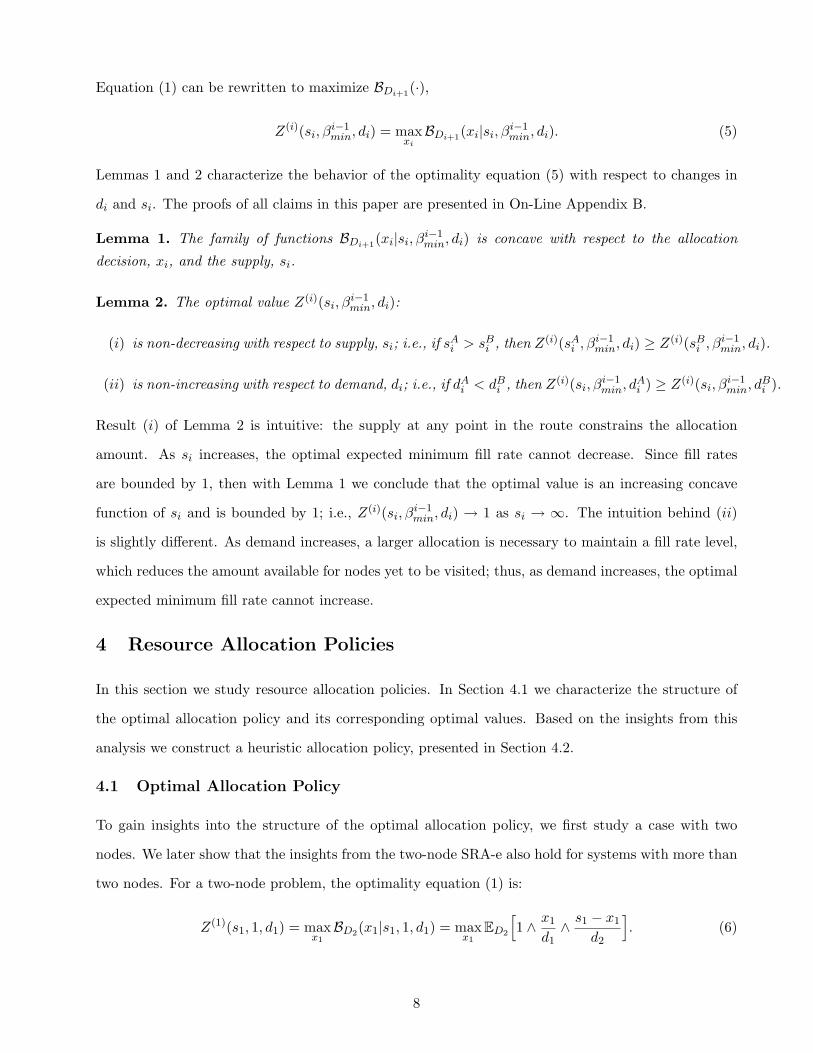
Equation (1) can be rewritten to maximize BDi+1(·),
Z(i)(si, βi−1min, di) = max
xi
BDi+1(xi|si, βi−1min, di). (5)
Lemmas 1 and 2 characterize the behavior of the optimality equation (5) with respect to changes in
di and si. The proofs of all claims in this paper are presented in On-Line Appendix B.
Lemma 1. The family of functions BDi+1(xi|si, βi−1min, di) is concave with respect to the allocation
decision, xi, and the supply, si.
Lemma 2. The optimal value Z(i)(si, βi−1min, di):
(i) is non-decreasing with respect to supply, si; i.e., if sAi > sBi , then Z(i)(sAi , βi−1min, di) ≥ Z(i)(sBi , β
i−1min, di).
(ii) is non-increasing with respect to demand, di; i.e., if dAi < dBi , then Z(i)(si, βi−1min, d
Ai ) ≥ Z(i)(si, βi−1
min, dBi ).
Result (i) of Lemma 2 is intuitive: the supply at any point in the route constrains the allocation
amount. As si increases, the optimal expected minimum fill rate cannot decrease. Since fill rates
are bounded by 1, then with Lemma 1 we conclude that the optimal value is an increasing concave
function of si and is bounded by 1; i.e., Z(i)(si, βi−1min, di) → 1 as si → ∞. The intuition behind (ii)
is slightly different. As demand increases, a larger allocation is necessary to maintain a fill rate level,
which reduces the amount available for nodes yet to be visited; thus, as demand increases, the optimal
expected minimum fill rate cannot increase.
4 Resource Allocation Policies
In this section we study resource allocation policies. In Section 4.1 we characterize the structure of
the optimal allocation policy and its corresponding optimal values. Based on the insights from this
analysis we construct a heuristic allocation policy, presented in Section 4.2.
4.1 Optimal Allocation Policy
To gain insights into the structure of the optimal allocation policy, we first study a case with two
nodes. We later show that the insights from the two-node SRA-e also hold for systems with more than
two nodes. For a two-node problem, the optimality equation (1) is:
Z(1)(s1, 1, d1) = maxx1
BD2(x1|s1, 1, d1) = maxx1
ED2
[1 ∧ x1
d1∧ s1 − x1
d2
]. (6)
8

Since the second node is the last node visited, its allocation is (s1 − x1) ∧ d2, which is the minimum
of available supply and observed demand. The objective function value of the entire sequence is:
Z(s1) = ED1
[Z(1)(s1, 1, d1)
]. (7)
The structure of the optimal allocation policy, x∗1, with respect to d1 and s1 is illustrated in Figure
3 for a two-node example where both nodes observe Normally distributed demand with µ = 60 and
σ = 18. The initial supply, s1, ranges from 10 to 250, and the observed demand at node 1, d1, ranges
from 13 to 103.
Figure 3: Optimal resource allocation policy x∗1 as a function of d1 and s1
From Figure 3, we see that x∗1 is non-decreasing in d1 for any value of s1. For each value of s1, x∗1
follows a piecewise function with respect to d1. The piecewise nonlinear structure has the following
property: there exists a value of demand, Td(s1), such that if d1 ≤ Td(s1) then x∗1 = d1. For any value
of d1 x∗1 is piecewise linear function of s1. For each value of d1, there exists a value of supply, Ts(d1),
such that if s1 < Ts(d1), then x∗1 is a linear function of s1; otherwise x∗1 = d1.
We prove these observations in Theorems 1 and 2. Theorem 1 characterizes the threshold structure
of the optimal solution with respect to demand at node 1, and Theorem 2 presents the sensitivity of
9

the optimal solution and objective value with respect to supply.
Theorem 1. (Structure of Optimal Resource Allocation Policy) In a two-node SRA-e problem,
for a given supply s1, the optimal allocation x∗1 is a piecewise function of d1. Specifically, there exists
a threshold, Td(s1), such that:
(i) if d1 ≤ Td(s1), then the optimal allocation, x∗1 = d1.
(ii) if d1 > Td(s1), then the optimal allocation, x∗1 = H1(s1, d1), where H1(s1, d1) < d1.
(iii) the threshold value, Td(s1), is non-decreasing in s1, and H1(s1, d1) is a strictly increasing concave
function of d1.
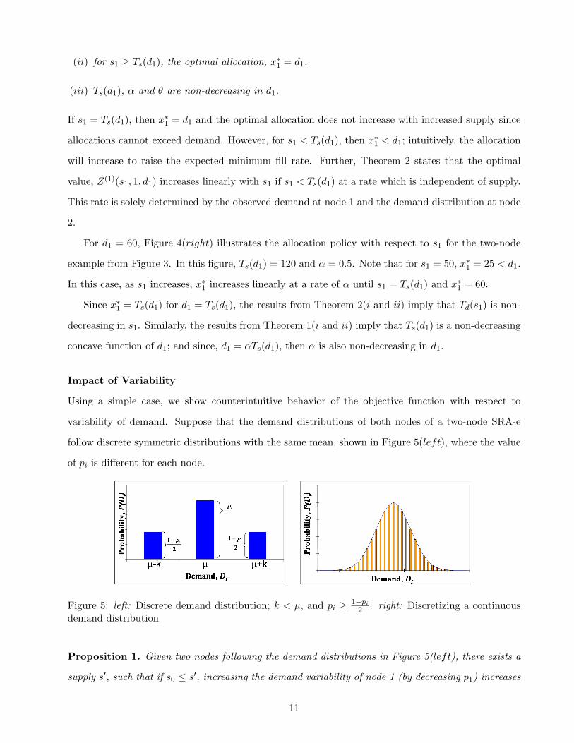
Figure 4: Optimal resource allocation policy (left) for a given value of s1 = 100 and (right) for agiven value of d1 = 60
For s1 = 100, the structure of the optimal allocation policy with respect to d1 is illustrated in Figure
4(left) for the two-node example in Figure 3. The threshold value is Td(100) = 45. If demand at
node 1 is relatively small (i.e., d1 ≤ Td(100) = 45), then demand at node 1 can be fully satisfied with
sufficient supply left to satisfy demand at the second node. For d1 > Td(100) = 45, it is not optimal
to fulfill node 1’s demand in full, x∗1 = H1(100, d1) < d1, and as d1 increases, supply must still be
held for the second node. Therefore, the allocation will not increase at the same rate as demand, and
H1(100, d1) is an increasing concave function of d1.
Theorem 2. (Sensitivity of the Optimal Resource Allocation Policy to Supply) In a two-
node SRA-e problem, for a given demand d1 there exists a supply level, Ts(d1), such that:
(i) for s1 < Ts(d1), the optimal allocation, x∗1 = H1(s1, d1) < d1, where H1(s1, d1) is an increasing
linear function of s1 (i.e., H1(s1, d1) = αs1). Furthermore, the optimal objective function value
at node 1, Z(1)(s1, 1, d1) is increasing with supply s1 at a constant ratio, θ.
10
(ii) for s1 ≥ Ts(d1), the optimal allocation, x∗1 = d1.
(iii) Ts(d1), α and θ are non-decreasing in d1.
If s1 = Ts(d1), then x∗1 = d1 and the optimal allocation does not increase with increased supply since
allocations cannot exceed demand. However, for s1 < Ts(d1), then x∗1 < d1; intuitively, the allocation
will increase to raise the expected minimum fill rate. Further, Theorem 2 states that the optimal
value, Z(1)(s1, 1, d1) increases linearly with s1 if s1 < Ts(d1) at a rate which is independent of supply.
This rate is solely determined by the observed demand at node 1 and the demand distribution at node
2.
For d1 = 60, Figure 4(right) illustrates the allocation policy with respect to s1 for the two-node
example from Figure 3. In this figure, Ts(d1) = 120 and α = 0.5. Note that for s1 = 50, x∗1 = 25 < d1.
In this case, as s1 increases, x∗1 increases linearly at a rate of α until s1 = Ts(d1) and x∗1 = 60.
Since x∗1 = Ts(d1) for d1 = Ts(d1), the results from Theorem 2(i and ii) imply that Td(s1) is non-
decreasing in s1. Similarly, the results from Theorem 1(i and ii) imply that Ts(d1) is a non-decreasing
concave function of d1; and since, d1 = αTs(d1), then α is also non-decreasing in d1.
Impact of Variability
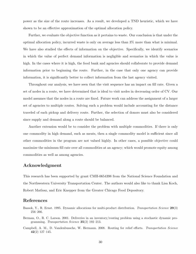
Using a simple case, we show counterintuitive behavior of the objective function with respect to
variability of demand. Suppose that the demand distributions of both nodes of a two-node SRA-e
follow discrete symmetric distributions with the same mean, shown in Figure 5(left), where the value
of pi is different for each node.
Figure 5: left: Discrete demand distribution; k < µ, and pi ≥ 1−pi
2 . right: Discretizing a continuousdemand distribution
Proposition 1. Given two nodes following the demand distributions in Figure 5(left), there exists a
supply s′, such that if s0 ≤ s′, increasing the demand variability of node 1 (by decreasing p1) increases
11

the expected minimum fill rate, where
s′ =2µ(2µ+ k)(p2µ+ k)
(1 + p2)(µ+ k)2 − (1− p2)µ2.
Proposition 1 claims that if s0 is less than threshold s′, then increasing the variability in demand in
node 1 improves the objective function, which is contrary to common intuition that demand variability
worsens system performance. In our SRA-e model, we observe several cases where increasing demand
variability leads to higher system performance. One reason for these dynamics is that low supply levels
result in low fill rates. In this case, increasing demand variability increases the probability of lower
demand observations, and therefore increases the expected fill rates. For high supply levels, lower
demand observations are satisfied fully resulting in a fill rate of 1, which is the maximum; therefore,
the solution does not benefit from the increased probability of lower demand values.
Note that by including more levels of demands, this discrete representation of a distribution in
Proposition 1 can be generalized to mimic the shape of symmetric unimodal continuous probability dis-
tributions as shown in Figure 5(right). While this exponentially increases the number of combinations
to consider in the analysis, it does not change the derived insight from Proposition 1.
Numerically solving for the optimal resource allocation policy for the SRA-e is computationally
intensive since the optimality equation, Z(i)(si, βi−1min, di), is evaluated for a three-dimensional state
space. To numerically evaluate Z(s0), it is necessary to discretize the state space. Let `s, `β and `d
represent the number of discretization intervals for supply, fill-rate and demands, respectively. The
number of intervals for the resource allocation (`xi) is dependent on supply, demand and fill-rate. If
si ≥ di, then `xi = `ββi−1min, since xi is constrained by the minimum fill rate and is chosen to meet the
fill rate intervals. If si < di, then xi is also limited by supply, thus `xi = `β(βi−1min∧
sidi
). For an N -node
SRA-e, at node N , there are `s`β`d possible states, and Z(N)(·) is determined with one computation for
each state since the optimal allocation policy is sN∧dN . For nodes 2 through N−1 there are also `s`β`d
possible states each, and Z(i)(·) is evaluated with `xi computations for each state to determine the
optimal allocation. For node 1, there are `d possible states since s1 = s0 and β0min = 1; the evaluation
of Z(0)(·) requires `x1 computations for each state to determine the optimal allocation. In total,
the number of computations needed to evaluate Z(s0) is equal to `d`x1 +∑N−1
i=1 (`s`β`d`xi) + `s`β`d.
For a three-node SRA-e, where supply and fill rate are discretized into 100 intervals and demand is
discretized into 20 intervals, the number of computations necessary to determine x∗1 and evaluate Z(s0)
12

is on the order of 108. Further, the computations needed to solve the dynamic program grow with the
number of nodes. This highlights the need for near-optimal heuristics that are easy to calculate. We
consider heuristic policies which produce allocation policies that mimic the structure of the optimal
policy and result in a near-optimal objective value.
4.2 Resource Allocation Heuristics
With the insights from two-node models, we develop a heuristic solution for the N -node problem
which we call the Two-node Decomposition (TND) heuristic. TND decomposes the N -node SRA-e
into sequential two-node problems; therefore, we first develop a two-node allocation heuristic.
4.2.1 Two-Node Problem
Based on Theorem 1, for a given supply at node 1 in a two-node problem, the optimal allocation policy
can be reasonably approximated by a piecewise function consisting of a linear function and a concave
function. Therefore, a two-node allocation heuristic policy at node 1, x1, would take on the structure:
x1 = min{H1(s1, d1), d1}, where H1(s1, d1) is an approximation of H1(s1, d1).
Suppose ρ is a forecast for demand at node 2. Using this forecast, our heuristic obtains H1(s1, d1)
by solving H1(s1,d1)d1
= s1−H1(s1,d1)ρ , which yields H1(s1, d1) = s1
d1d1+ρ . We plot x1 as a function of d1 in
Figure 6 for s1 = 100 and an arbitrary value for ρ; i.e., ρ = 55.
Figure 6: Heuristic allocation policy
The heuristic allocation curve in Figure 6 is similar in shape to the optimal allocation curve in
Figure 4(left). Note that if forecast ρ is accurate (i.e., ρ is exactly equal to the demand at node 2),
then our heuristic results in the optimal allocation policy (i.e., H1(s1, d1) = H1(s1, d1)). If one cannot
guarantee a precise value for ρ, which is generally the case, one must choose ρ such that H1(s1, d1)
approximates H1(s1, d1) as accurately as possible.
13

It is clear that ρ depends on the magnitude of and variability in the demand of node 2. Our
heuristic bases the value of ρ on the median of the demand (m2), to capture the magnitude, adjusted
by a correction factor (δ2√σ2), to account for demand variability. Specifically, ρ is calculated as
follows: ρ = m2 + δ2√σ2, where δ2 = m1−m2
avg(m1,m2) , which is the difference between median demands
standardized by the average median demand.
The correction factor (δ2√σ2), consists of σ2 to account for demand variability in node 2, and δ2
to account for dissimilarity in the demand magnitude between nodes 1 and 2. Dissimilarity in the
demand magnitude affects fill rate value of supply at each node. For example, if demand at node 1 is
significantly lower than that at node 2, then increasing the allocation to node 1 by one unit has more
impact on its fill rate than increasing the allocation to node 2 by one unit. In this case the correction
factor would be negative, since m1 < m2, to reduce the value of ρ. Similarly, if the demand magnitude
at node 1 is significantly greater than that at node 2, then the fill rate value of supply at node 2 is
greater and the correction factor would increase the value of ρ.
From numerical studies, we find that basing ρ on median is more effective than basing ρ on mean
for a wider variety of demand distributions. For example, if the demand at node 2 is strongly skewed
to the left, the probability of demand being significantly more than µ is much larger than 0.5. Basing ρ
on mean would assign too small a weight on node 2’s demand and therefore, allocate too much to node
1. However, when ρ is based on median, regardless of the shape of the distribution, the probability
that the demand be smaller or larger than median is always 0.5, so the inventory reserved for node 2
will not be too large or too small. A similar argument holds for demand distributions that are skewed
to the right. For symmetric distributions, using median is identical to using the mean.
The complete two-node allocation heuristic can be written:
x1 = min{H1(s1, d1), d1} (8)
H1(s1, d1) = s1d1
d1 + (m2 + δ2√σ2)
(9)
4.2.2 N-Node Problem
The TND heuristic consists of three phases:
Phase 1. Decomposition: The N -node problem is decomposed into sequential two-node problems.
For example, at node 1, the TND heuristic solves a two-node SRA-e consisting of nodes 1 and 2.
At node 2, the method solves another two-node SRA-e consisting of nodes 2 and 3, and so on.
14

Phase 2. Supply Allotment: For each sequential two-node SRA-e, the available supply is divided
so that one portion is allotted to solve the two-node problem and the other is reserved for the
other nodes not yet visited. For example, for N = 5, a portion of s1 is allotted for the two-node
problem for nodes 1 and 2, and the rest is reserved for nodes 3, 4 and 5. At node 2, a portion of
s2 is alloted for the two-node problem for nodes 2 and 3, and the rest is reserved for remaining
nodes 4 and 5, and so on. The allotment (si) for the two-node SRA-e for nodes i and i + 1 is
determined by:
si = siµi + µi+1∑N
j=i µj(10)
At each visit, si is calculated so that an appropriate amount of supply is available for allocation
to the two-node problem i and i + 1. The fraction of available supply si that is allotted to the
two-node problem, si, is proportional to the average demand of the two node relative to the total
average demand of the unvisited nodes. Note that, although one can also base the allotment on
median, we observed in our numerical study that using medians instead of means to determine
supply allotments reduces the effectiveness of the TND algorithm.
Phase 3. Resource Allocation: For each sequential two-node problem consisting of nodes i and
j with the alloted supply si determined by (10), the two-node allocation heuristic is used to
determine the allocation amount:
xi = min{Hi(si, di), βi−1mindi} (11)
Hi(si, di) = sidi
di + (mi+1 + δi+1√σi+1)
(12)
Note that (11) includes the term βi−1min, the minimum fill rate among nodes visited, which differs
from (8). In the N -node problem, βi−1min depends on the observed demand and allocation decisions
at nodes 1 to i − 1; in the two-node problem, β0min = 1. Allocation according to (11) implies
that there is no incentive to allocate an amount that will result in a higher fill rate than βi−1min,
which is the current minimum fill rate since the objective is to maximize the minimum fill rate
of the entire sequence. One would rather reserve supply to address future demand volatility.
The TND heuristic algorithm begins at node 1 with initial supply, s0, and steps through the three
phases as each node is visited. The following is a complete description of the algorithm:
15

TND Heuristic Allocation AlgorithmStep 0: Initialize i = 1, s1 = s0 and β0
min = 1.Step 1: Determine supply allotment, si, using si = si
µi+µi+1∑j=i...N µj
.
Step 2: Determine resource allocation, xi, for the two-node problem for nodes i andi+ 1 after observing di: using xi = min{Hi(si, di), βi−1
mindi}, whereHi(si, di) = si
didi+(mi+1+δi+1
√σi+1) .
Step 3: Update βimin = βi−1min ∧
xidi
and si+1 = si − xi.Step 4: If i + 1 < N , then set i = i + 1 and go to Step 1. Else i + 1 = N STOP;
xN = sN ∧ dN .
Note that the TND heuristic algorithm reduces to the two-node allocation heuristic when N = 2.
4.2.3 Excess Priority and Excess Sharing Heuristics
We evaluate the performance of the TND heuristic against the optimal allocation policy, as well as
four heuristic allocation policies developed as benchmarks to evaluate the performance of our TND
heuristic: (i) Excess Priority heuristic based on mean, (ii) Excess Priority heuristic based on median,
(iii) Excess Sharing heuristic based on mean, and (iv) Excess Sharing heuristic based on median. All
of these heuristics consider a threshold value κi for node i, and allocate inventory xi to node i as
follows:
xi ={di : if di ≤ κiκi : if di > κi
Excess Priority Heuristic Based on Mean:
Under this heuristics, initial values for thresholds κ(o)i , for all i, are calculated based on the mean of
demand at all nodes as follows:
κ(o)i = s0
µi∑Nj=1 µj
. (13)
These initial thresholds are updated after the demand at a node is observed. Specifically, after visiting
node i, if there is excess supply (i.e., if node i requests less than its assigned threshold), then the
excess is available immediately for allocation to node i + 1. Under Excess Priority heuristics, after
allocation at node i, only the threshold value at node i + 1 is updated. More formally, suppose that
κ(i)i+1 is the updated threshold at node i+ 1 after nodes 1 to i are visited. Then, after visiting node i,
the value of κ(i)i+1 for node i+ 1 is obtained as follows:
κ(i)i+1 =
{κ
(o)i+1 + (κ(i−1)
i − di) : if di ≤ κ(i−1)i
κ(o)i+1 : if di > κ
(i−1)i
Note that, upon arrival to node i+ 1, the heuristic tends to allocate all the excess (unused) supply at
node i (i.e., κ(i−1)i − di) to node i + 1 by increasing the initial threshold at node i + 1 from κ
(o)i+1 to
16

κ(o)i+1 + (κ(i−1)
i −di). If there is no excess supply at node i, then the initial allocation threshold at node
i+ 1 does not change.
The Excess Priority Heuristic Based on Median is analogous to the above, except median mi is
used in place of mean µi for all i = 1, 2, . . . , N .
Excess Sharing Heuristic Based on Mean:
The Excess Sharing Heuristics use the same initial values for threshold as in (13). However, after
visiting node i, if there is excess supply (i.e., if the demand in node i is less than its assigned thresh-
old), then the excess is shared among all remaining nodes, by revising all thresholds in those nodes.
Specifically, after visiting node i, the thresholds κ(i)j are revised for all nodes j = i+ 1, i+ 2, . . . , N as
follows:
κ(i)j =
κ(i−1)j + (κ(i−1)
i − di) µj∑Nk=i+1 µk
: if di ≤ κ(i−1)i
κ(i−1)j : if di > κ
(i−1)i
The Excess Sharing Heuristic Based on Median is analogous to the above, except median mi is used
in place of mean µi for all i = 1, 2, . . . , N .
4.2.4 Performance Evaluation of Allocation Heuristics
In the numerical study, we evaluate the performance of our TND, excess priority, and excess sharing
heuristics with that of the optimal allocation policy
In our numerical studies, we consider instances with 2 to 7 nodes. In the FRP, the majority of routes
visit 7 agencies or less. Demands are observed from gamma distributions, which allow the modeling of
settings with low and high variability corresponding to coefficient of variation (CV) less and greater
than 1. Demand distributions are discretized into equally spaced intervals and all possible sample
paths are enumerated to calculate the performance of each allocation policy. Table 1 summarizes the
SRA-e scenarios in our analysis, which can be organized into three categories.
Node sets A to D consist of nodes with identical demand means, either low (50) or high (150).
The CVs of the demand within the sets are uniformly distributed over a range. We consider a wide
range of CV (0.5 - 1.5) and a narrow range (0.75 - 1.25). For example, for an instance with 5 nodes
with the wide range of CV, the CV’s assigned to the 5 nodes are 0.5, 0.75, 1.0, 1.25, and 1.5. For
node sets A to D, we consider five sequences: The CV↗ sequence visits nodes in order of lowest to
highest CV, and the CV↘ sequence visits nodes in order of highest to lowest CV. The CV ∧ sequence
places the higher CV nodes in the middle of the route and the lower CV nodes at the beginning and
17

Node set µ CV SequencesA 50 0.5 - 1.5
CV↗, CV↘, CV ∧, CV ∨, CV ∼B 150 0.5 - 1.5C 50 0.75 - 1.25D 150 0.75 - 1.25E 50 - 150 0.5
µ↗, µ↘, µ∧, µ∨, µ∼F 50 - 150 1.5G 75 - 125 0.5H 75 - 125 1.5
I 50-1500.5 - 1.5
CV↗, CV↘, CV ∧, CV ∨, CV ∼Large µ with large CV
J 50-1500.5 - 1.5
Large µ with small CV
Table 1: SRA-e scenarios in numerical study
end of the routes. The CV ∨ sequence is the opposite, where the higher CV nodes are at the beginning
and end of the routes, and lower CV nodes are in the middle of the route. Finally, the CV ∼ sequence
alternates the nodes with low and high CV.
Node sets E to H consist of nodes with identical CV, either low (0.5) or high (1.5). The mean
demand within the node sets are uniformly distributed over a wide range (50 - 150) or narrow range
(75 - 125). We consider five sequences: µ↗, µ↘, µ∧, µ∨ and µ∼ which follow the same sequencing
logic as CV sequencing.
Node sets I and J, consist of nodes with different µ and CV; µ is uniformly distributed from 50 to
150 and CV is distributed from 0.5 to 1.5. In node set I, the nodes with large µ have high CV and
in node set J, the nodes with large µ have low CV. For both sets, we consider the same sequences as
node sets A to D.
We consider the five sequences for each of the ten node sets in Table 1, resulting in 50 different
routes for instances with 3 to 7 nodes. In two-node instances there are only two possible sequences
resulting in 20 different routes. For each of these 270 routes, we consider five levels of initial supply
ranging from 0.5 to 1.5 times the total mean demand of the nodes in a route (i.e.,∑N
i=1 µi). In total,
our study evaluates each allocation policy in 1,350 different scenarios.
Let gH represent the objective value for the TND heuristic, and let gµ and gm represent the
objective values for the corresponding mean and median allocation heuristic policies, respectively.
Table 2 lists the average and maximum optimality gaps (i.e. Z − gh) for the five policies considered.
In our numerical analysis we observe the following:
18

TND Excess Priority Excess SharingNumber of Z − gH Z − gµ Z − gm Z − gµ Z − gm
nodes Avg Max Avg Max Avg Max Avg Max Avg Max2 0.6% 2.6% 3.0% 15.5% 4.9% 23.9% 3.0% 15.5% 4.9% 23.9%3 0.7% 3.0% 4.7% 12.7% 6.8% 26.9% 5.4% 13.2% 8.4% 27.7%4 0.8% 2.9% 6.2% 13.5% 7.7% 29.8% 8.1% 14.7% 10.3% 31.9%5 1.2% 3.2% 7.6% 14.0% 9.1% 33.4% 10.5% 18.0% 12.9% 37%6 1.7% 4.2% 8.8% 14.5% 10.4% 36.1% 12.8% 21.0% 15.2% 40.8%7 2.3% 4.9% 9.8% 15.5% 11.5% 37.2% 14.8% 23.7% 17.2% 43.0%
Total 1.3% 4.9% 7.1% 15.5% 8.8% 37.2% 9.1% 23.7% 11.5% 43.0%
Table 2: Average and maximum optimality gaps
• For all policies, the average optimality gaps increase with the number of nodes. On average,
the TND heuristic is within 1.3% of the optimal allocation policy and at worst less than 5%
from optimal for routes up to seven nodes. The TND heuristic errors trend upward for larger
problems; however, the heuristic’s performance is significantly better than that of the other four
heuristics in most cases.
• In a direct comparison, the TND heuristic is, on average, 5.8% and 7.5% better than the excess
priority mean and median objectives, respectively, with maximum differences of 15.4% and
32.3%. Even though the differences between the TND heuristic and excess priority median
heuristic is large, there are cases in which the excess priority median heuristic results in a higher
objective than the TND heuristic. These cases are typically in node sets A, B, I and J with the
CV↗ sequence. The differences are, on average, less than 0.5% and as high as 1.5%, which are
relatively small when compared to the difference in cases where the TND heuristic is better. For
node sets A, B, I and J, where nodes are visited in CV↗ sequence, the optimality gap of the
excess priority median heuristic is much smaller than the aggregated results in Table 2. For these
scenarios, the average gaps range from 0.7% for a two-node problem to 3.7% for a seven-node
problem. Therefore, in these cases, both the excess priority median and the TND heuristic are
effective approximations for the optimal policy.
• The excess priority mean and median heuristics are, on average, 2.0% and 2.7% better than the
excess sharing mean and median heuristics, respectively. This may seem counterintuitive since
the excess sharing policy seems more equitable as it redistributes the excess supply among all
nodes not yet visited. However, this redistribution is calculated based on the assigned thresholds
that may not be optimal. Therefore, it is better to use the excess supply as needed now (when the
19

demand is realized) rather than redistributing the excess among remaining nodes, expecting that
they will definitely be needed later in the remaining nodes. This, as we observed in our numerical
study, leads to excess priority heuristic producing less waste than excess sharing heuristic, and
therefore a more effective inventory allocation.
In Table 3, we present the average and maximum optimality gaps, as well as the percent of cases
in which the TND objective is within 2% of the optimal value for each node set. The detail results
for Excess Priority and Excess Sharing heuristics are presented in On-Line Appendix A. The TND
heuristic performs within 2% of the optimal allocation policy for a significant majority of cases. For
scenarios with higher demand variability (sets B, F, H, I and J), the gaps are slightly higher. The
sharpest comparison is the difference between sets E and G to F and H, respectively, which are sets
with the same mean but with different CV. The TND heuristic is based on approximating demand,
and therefore will have lower optimality gaps for settings with more predictable demand such as in
sets E and G. However, for settings with more demand variability as in sets F and H, the average
optimality gap is less than 2% and in 77% of the cases in these two sets, the performance of the
heuristic is within 2% of that of the optimal allocation policy.
A B C D E F G H I JAverage optimality gap 1.1% 1.2% 1.1% 1.1% 0.8% 1.8% 0.7% 1.8% 1.4% 1.2%
Maximum optimality gap 3.6% 3.7% 3.1% 3.0% 3.2% 4.9% 2.6% 4.2% 4.3% 4.4%% of cases gap ≤ 2% 93% 88% 91% 91% 97% 83% 99% 71% 87% 90%
Table 3: TND heuristic optimality gaps by node sets
The numerical studies show that the TND heuristic determines an allocation policy which results
in significantly better objective values than the benchmark policies. The heuristic’s objective is within
2% of an optimal allocation policy in about 90% of the cases. Although the gaps of the TND heuristic
increase with route size, they remain significantly better than the benchmark heuristics errors which
increase at a higher rate. Given the service time at a node and the travel time between nodes, many
pick-up and delivery applications are limited in the number of stops per route, see pickup and delivery
test cases presented in Savelsbergh and Sol (1995). Service times in the FRP are approximately 10-20
minutes for donors and 15-30 minutes for agencies, and travel distances between nodes are between 10
to 20 minutes. It is easy to see that routes are not likely to visit more than 7 agencies, since donors
must be visited on routes as well. Our heuristic is valuable as well in applications with many nodes
per route, since the computational complexity does not allow one to compute the optimal allocation
20

policy.
5 Sequencing Policies
Sequencing nodes in the SRA-e along a route impacts the expected minimum fill rate, as shown in
Section 4. In the case of the FRP, this can also impact the distance traveled and the associated travel
cost. However, if travel costs are low compared to stopping costs, or if all locations are located in
a dense area (such as the agencies in Figure 1), then the total distances or costs of the visitation
sequences do not differ significantly. In such settings, it may be beneficial to find the best sequence of
nodes that optimizes the fill rate objective.
The impact of sequencing can be significant; consider the example in Figure 2. Let the demand at
node 1 remain the same, but the demand at node 2 be either 10 or 90 with equal probability. When
node 1 is visited first, given s0 = 130, we have Z = 70%. If node 2 is visited first, then Z = 82%
which is 12% higher. This is a simple example that shows sequencing can have a significant impact
on the objective value. In this section, we address the sequencing decision when given a set of nodes
to visit. We begin with a study of optimal sequencing policies for special cases in Section 5.1. Based
on these results we construct a sequencing heuristic for general problems, which we present in Section
5.2.
5.1 Optimal Sequencing Policy
To investigate the impact of mean on the optimal sequence, we first study a two-node problem where
nodes observe demands from the same family of distributions with different means, but with identical
standard deviations. In this case, we are able to show that it is optimal to sequence the node with
lower demand mean first.
Theorem 3. In a two-node SRA-e problem in which two nodes observe demand from the same family
of distributions with different means, but with identical standard deviations, visiting the nodes in
increasing order of demand mean will result in a higher expected minimum fill rate.
We now consider a case where nodes observe demand from distributions with identical means but
different standard deviations, such as the discrete demand distribution in Figure 5(left) in Section
4.1.
21

Theorem 4. In a two-node SRA-e problem in which two nodes follow the demand distributions in
Figure 5(left), if p1 < p2, then the expected minimum fill rate is greater when node 1 (which has a
higher standard deviation) is visited first.
Theorem 4 suggests that it is optimal to sequence the nodes in decreasing order of standard
deviation. This result is not surprising; it is intuitive that visiting the node with higher demand
variability first is preferable. This sequencing minimizes the effect of variability, since the demand at
the first node is observed and the uncertainty arises from the second node which has more predictable
demand.
In Theorem 3, the demand variability of both nodes are identical in an absolute sense, since they
have identical standard deviation. However, their coefficient of variations (CV), a measure of relative
demand variability, differ since the distributions have different means. The node with the smaller
mean has higher CV, and thus higher relative demand variability. The result in Theorem 3 implies
that it is better to visit the node with higher relative demand variability first, which is consistent with
the insight from Theorem 4.
Both Theorem 3 and 4 imply that relative CV can be a good rule for sequencing nodes. This
principle of sequencing in decreasing order of CV is extended to more general problems next.
5.2 Sequencing Heuristic
Following Theorems 3 and 4, we define the following routing heuristic for more general problems.
Sequencing Heuristic: Sequence nodes in decreasing order of CV. If CV’s are identical, sequence
nodes in decreasing order of standard deviation.
We test the sequencing heuristic in two- to six-node instances with node sets described in Table 1
under the optimal resource allocation policy. For a N -node problem, the optimal sequence is found
by comparing the objective function of all N ! sequences under their corresponding optimal allocation
policies. Therefore, we limit the tests to routes of six nodes or less. We consider five supply levels
for the 10 node sets, resulting in 50 cases for each route size. In total, we evaluate the sequencing
heuristic in 250 different scenarios. The results are summarized in Table 4.
The first row in Table 4 presents the percent of cases in which the heuristic determines the optimal
sequence. The second row presents the percent of cases in which the difference between expected
minimum fill rate of the heuristic sequence and that of the optimal sequence is less than 1%. Lastly,
22

Number of nodes2 3 4 5 6 Total
Optimal sequence chosen 64% 50% 44% 44% 32% 47%Within 1% of optimal sequence 96% 96% 98% 100% 100% 98%
Maximum optimality gap 1.5% 1.3% 1.1% 0.9% 0.8% 1.5%
Table 4: Effectiveness of the sequencing heuristic
the third row presents the maximum difference in objective function value between the sequencing
heuristic and optimal sequence.
In general, in 47% of cases, the sequencing heuristic chooses the optimal sequence. These cases
are typically in routes where nodes vary in CV; i.e., A, B, C, D, I and J. In these sets, the sequencing
heuristic chooses the optimal sequence in 75% of cases. For node sets where nodes have identical CV
(sets E, F, G and H), the sequencing heuristic chooses the optimal sequence in only 4% of these cases.
However, the heuristic chooses a sequence within 1% of the optimal 98% of the time and the maximum
difference in objective for all cases is 1.5%. These results confirm that the sequencing heuristic is an
effective method to determine a near-optimal visitation sequence.
6 Resource Allocation Heuristic with Sequencing Heuristic
In this section, we evaluate the performance of our sequencing and TND heuristics when used together
to solve the SRA-e problem. For each node set described in Table 1, we determine the optimal sequence
under optimal allocation and calculate the optimality gap in expected minimum fill rate from: the
same optimal sequence under our TND heuristic (SeqoptAllocheu), our heuristic sequence under optimal
allocation (SeqheuAllocopt), and our heuristic sequence under our allocation heuristic (SeqheuAllocheu).
The results for two- to six-node problems, averaged over supply levels for each node set, are shown in
Table 5.
Number of SeqoptAllocheu SeqheuAllocopt SeqheuAllocheunodes Avg Max Avg Max Avg Max
2 0.5% 2.6% 0.2% 1.5% 1.0% 2.6%3 0.6% 1.8% 0.2% 1.3% 0.8% 2.0%4 1.0% 2.6% 0.2% 1.1% 0.9% 1.7%5 1.5% 3.0% 0.2% 0.9% 1.3% 2.1%6 2.1% 4.2% 0.2% 0.8% 1.8% 3.3%
Total 1.1% 4.2% 0.2% 1.5% 1.2% 3.3%
Table 5: Average and maximum optimality gaps
The results for SeqoptAllocheu consider only one sequence (i.e., the optimal sequence), and thus
23

differ from the results in Table 2 that are averages over five sequences. The optimality gap values for
SeqoptAllocheu are consistent with those from Table 2, with low average and maximum values at 1.1%
and 4.2%, respectively. The results for SeqheuAllocopt are from the same data summarized in Table
4; here, we include the averages. The average and maximum optimality gaps for SeqheuAllocheu are
1.2% and 3.3%, respectively. These values are not significantly different from the gap values when
only one heuristic is implemented, thus there is no compounding effect in combining the heuristics.
We can conclude that combining the sequencing and TND heuristics results in near optimal solutions.
7 Value of Information
In some applications, it may be possible to obtain demand information prior to visiting the first node.
In this section, we evaluate the benefit of advanced demand information. In Section 7.1, we compare
the performance of the SRA-e in the case of unknown demands with the case where all demands are
known (complete information). In Section 7.2, we consider a setting where demand information is
only available from a single node (partial information).
7.1 Complete Information
Let υc represent the value of complete information: the absolute difference between the objective
value when the demand at all nodes are known before visiting the first node and when demand is
revealed only upon arrival at a node. We limit the numerical study to routes of six nodes and compute
the maximum expected minimum fill rates for the routes described in Table 1, for a total of 250
scenarios. From our results, the average and maximum value of υc over all scenarios is 9.1% and
18.7%, respectively. The average value of complete information is between 9% and 10% for each node
set except E and G, where the average υc is 6.8%, due to the low CV values in these sets. Based on
the data, we make the following observations:
Observation 1. The value of complete information (υc) is increasing with increasing variability of
demand (i.e., CV) at all nodes. Furthermore, the value of information is decreasing as the initial
supply (s0) becomes very large or very small.
Observation 2. For a given set of nodes, the maximum value of complete information (υc) is obtained
when the nodes are sequenced in increasing order of demand variability.
As an example, consider scenarios in node set E and G with supply greater than the average demand
24

of the route. The average value of complete information is only 1.2% and at most 2.5%. In such
scenarios, obtaining complete information does not provide significant benefit. In contrast, consider
scenarios in node sets A, B, C, D, F, H, I and J with supply lower than the average demand of the
route, and routed in either CV↗ or µ↗. The average value of υc is 16.6% and at most 18.7%. In these
cases, obtaining complete information significantly improves the objective of maximizing the expected
minimum fill rate.
The intuition behind Observation 1 is as follows. It is clear that the value of information increases in
variability in demand, since as the variability in demand increases, predicting demand in nodes becomes
more difficult. To understand the impact of initial supply on the value of information, consider an
extreme case that the initial supply is very limited, e.g., s0 = 2 and the average demand in each node
of a three-node problem is µi = 100 for i = 1, 2, 3. Note that, in this case, having complete demand
information does not have much impact on the allocation decision, since the minimum expected fill
rate would be zero, regardless of whether the demand information is utilized or not. However, as
the initial supply increases, the demand information becomes more useful, and therefore the value of
information increases. The value of information starts to decreases as the initial supply becomes very
large. Consider the above example, and assume that the initial supply is s0 = 10, 000 instead of two.
It is clear that the value of information is almost zero. Since ample supply is available for all nodes, the
optimal decision is to allocate to each node whatever it requests, regardless of the demand information
of remaining nodes. Therefore, the value of information decreases as initial supply becomes very large
or very small.
Observation 2 states that the value of complete information is highest when nodes are sequenced
in increasing order of demand variability. Note that when making an allocation decision at node i, the
decision maker faces the uncertainty in demands in nodes i + 1 to N . When nodes are sequenced in
increasing order of demand variability, the decision making at each node i (i = 1, 2, . . . , N) involves
more uncertainty compared to that of any other sequencing of nodes. Higher uncertainty corresponds
to a higher value of information. Thus the value of information is highest in cases where nodes are
sequenced in increasing order of demand variability.
7.2 Partial Information
In practice, it may be difficult to obtain demand information from all nodes. For example, in the
FRP, obtaining demand information is difficult due to lack of personnel and the timing of delivery
25

operations. It is more likely that demand information can be obtained from one or two nodes. We
consider strategies of obtaining demand information from only one node and evaluate the portion of
υc which is captured by observing demand from a single node. We address the following questions for
the same six-node routes used in the numerical study for complete information:
1. Which position along the route provides the most valuable demand information? This excludes
the first node, since its demand is known immediately before any decision is made.
2. Do the demand characteristics such as average demand (µ) and coefficient of variation (CV) of
a node have an impact on the value of its demand information?
In answering question 1, for each node position along the route, we calculate the maximum expected
minimum fill rate if demand from that node is obtained. Figure 7 presents the average objective values,
from scenarios with node sets A-E, where information is obtained from the ith node in the route, from
no nodes and from all nodes. The results for node sets F-J are similar.
Figure 7: Average objective values for information from different node positions, node sets A-E
From Figure 7, we see that, on average, υc is at least 6% greater than the value of obtaining
information from a single node. We define the value of partial information (υp), as follows:
υp =gc − gpυc
,
26

where υp represents the portion of υc captured and where gp and gc represents the objective value
for the scenario with partial and complete information, respectively. For the sixth position, υp is on
average 30% which is greater than obtaining information from any other position. In other words,
one can obtain, on average, 30% of the value of complete information if one receives information only
from the last node in the sequence. Further, we are able to make the following observation:
Observation 3. In general, the value of demand information from one node (υp) is greater than that
of another node if it is visited later in the sequence.
By this observation, it is best to obtain information from the farthest position in a route as possible.
The intuition is that the information from nodes at the end of a route are useful in more decisions than
information from nodes at the beginning of the route. For our six-node problem, information from the
sixth node is used in decisions at the first through fifth nodes, while information at the second node
is only useful in the allocation decision at the first node.
In answering question 2, from Figure 7, we also see that υp is greater if the node providing
information has higher demand variability. For example, consider the ↘ and ∧ sequences (for both µ
and CV), where the node with the highest variability is sequenced third. In Figure 7, we see that υp
for the third position is greater in these two sequences than in the other three sequences. Similarly,
we see that if information was obtained from the fourth position, υp is highest for the ∧ sequence, and
by contrast is lowest for the ∨ sequence.
To further investigate the impact of a node’s demand characteristics, we consider obtaining demand
information from nodes with the following: largest and smallest µ, and largest and smallest CV . Note
that for µ, node sets A-D are not considered since nodes have identical µ; and for CV, node sets E-H
are not considered since nodes have identical CV. We present the average υp of each characteristic in
Table 6.
Information from node with . . .Sequence Highest µ Lowest µ Highest CV Lowest CV↗ 34.6% 5.0% 31.8% 3.8%↘ 12.5% 16.0% 5.9% 24.2%∧ 21.6% 20.8% 16.1% 25.4%∨ 34.0% 9.4% 36.3% 6.8%∼ 5.4% 5.0% 5.2% 6.4%
Total 21.6% 11.2% 19.1% 13.3%
Table 6: Average υp captured by each case
27

From the results in Table 6, we make the following observation:
Observation 4. The demand characteristics of a node have an impact on its value of demand in-
formation; its value is higher if the node has higher µ or higher CV relative to other nodes in the
sequence.
As an example, consider the ↗ and ↘ sequences. In the ↗ sequence, the nodes with the highest µ
and CV are positioned last in the sequence; while in the ↘ sequence, the nodes with the smallest µ
and CV are positioned last in the sequence. On average, the difference of υp between ‘Highest µ’ for
↗ and ‘Lowest µ’ for↘ is 34.6%−16.0% = 18.6%, which implies that the last node’s µ has an impact
on υp. In addition, the average difference of υp between ‘Highest µ’ for ↘ and ‘Lowest µ’ for ↗ is
12.5%− 5.0% = 7.5%; therefore, the value υp is higher if the demand information is from a node with
higher µ. Similar results hold for CV, and for the ∧ and ∨ seqeunces.
In conclusion, in scenarios with low CV and high supply the value of information is minimal, in
all other scenarios the objective can be improved by obtaining demand information. The greatest
impact of information is in scenarios with high CV, low supply and routed in increasing order of
demand variability. The benefit may be as high as an 18.7% increase in expected minimum fill rate. If
information can only be obtained from one node, the value of information is maximized if the node is as
far along in the sequence as possible. The benefit from obtaining information from the last sequenced
node is as high as an 7.2% increase in expected minimum fill rate. The value of information can be
further improved if the selected node has higher µ or CV relative to other nodes in the sequence.
8 Expected Waste
In the FRP, the food distributed is perishable and considered wasted if not distributed. Along with
the objective of promoting equity, minimizing waste is also a goal. In this section, we compare the
expected waste under an objective that maximizes the expected minimum fill rate with that under an
allocation policy that minimizes the expected waste.
We measure waste as the percentage of s0 that is not distributed to nodes. The waste minimization
allocation policy allocates the maximum possible amount at each node so to minimize the amount of
undistributed supply. The expected waste under an allocation policy is calculated through a computer
program that generates all sample paths of demand realizations. In Table 7, we present the average
28

difference in the expected minimum fill rate and expected waste for the two policies. Let Z and ω
represent the expected minimum fill rate and expected waste from the fill rate objective, respectively,
and let gW and ωW represent the expected minimum fill rate and expected waste from the waste
objective, respectively.
Fill rate optimality gap Expected waste optimality gapNumber of nodes Z − gW ω − ωW
2 8.0% 1.2%3 11.9% 1.7%4 13.1% 2.4%5 14.5% 2.7%6 15.5% 3.1%7 16.3% 3.4%
Total 13.2% 2.4%
Table 7: Average difference in expected minimum fill rate and expected waste between fill rate andwaste policies
From the results in Table 7, we make the following observation:
Observation 5. The optimal allocation policy for the objective of maximizing the expected minimum
fill rates results in close-to-minimal expected waste levels.
The results show that operating under the optimal resource allocation policy results in 2.4% more
expected waste, on average, then the minimal waste allocation policy. This is relatively small when
compared to the poor performance in expected minimum fill rate of the waste minimization policy.
Under a waste minimization policy the expected minimum fill rate is on average 13.2% worse than
that of the optimal value. This is not surprising, since the waste minimization objective produces
an extreme allocation policy which ignores fill rates. The optimal resource allocation policy produces
only 2.4% additional waste; therefore, following the objective of maximizing the expected minimum
fill rates keeps waste at a level close to the minimum.
9 Conclusion
In this paper we address design and operating policies of a nonprofit sequential resource allocation
problem. Motivated by the goal of the GCFD to provide equitable service while maintaining a high
level of distribution to its agencies, we defined the allocation objective to maximize the expected
minimum fill rate. Because of the complexity of the objective, it is not possible to derive a closed form
solution; further, solving for optimal allocations with dynamic programming requires more computing
29
power as the size of the route increases. As a result, we developed a TND heuristic, which we have
shown to be an effective approximation of the optimal allocation policy.
Further, we evaluate the objective function as it pertains to waste. Our conclusion is that under the
optimal allocation policy, incurred waste is only on average less than 3% more than what is minimal.
We have also studied the effects of information on the objective. Specifically, we identify scenarios
in which the value of perfect demand information is negligible and scenarios in which the value is
high. In the cases where it is high, the food bank and agencies should collaborate to provide demand
information prior to beginning the route. Further, in the case that only one agency can provide
information, it is significantly better to collect information from the last agency visited.
Throughout our analysis, we have seen that the visit sequence has an impact on fill rate. Given a
set of nodes in a route, we have determined that is ideal to visit nodes in decreasing order of CV. Our
model assumes that the nodes in a route are fixed. Future work can address the assignment of a larger
set of agencies to multiple routes. Solving such a problem would include accounting for the distance
traveled of each pickup and delivery route. Further, the selection of donors must also be considered
since supply and demand along a route should be balanced.
Another extension would be to consider the problem with multiple commodities. If there is only
one commodity in high demand, such as meats, then a single commodity model is sufficient since all
other commodities in the program are not valued highly. In other cases, a possible objective could
maximize the minimum fill rate over all commodities at an agency; which would promote equity among
commodities as well as among agencies.
Acknowledgment
This research has been supported by grant CMII-0654398 from the National Science Foundation and
the Northwestern University Transportation Center. The authors would also like to thank Lisa Koch,
Robert Matlosz, and Eric Knepper from the Greater Chicago Food Depository.
References
Bassok, Y., R. Ernst. 1995. Dynamic allocations for multi-product distribution. Transportation Science 29(3)256–266.
Berman, O., R. C. Larson. 2001. Deliveries in an inventory/routing problem using a stochastic dynamic pro-gramming. Transportation Science 35(2) 192–213.
Campbell, A. M., D. Vandenbussche, W. Hermann. 2008. Routing for relief efforts. Transportation Science42(2) 127–145.
30

Chou, M., C. Teo, H. Zheng. 2008. Process flexibility revisited: Graph expander and food-from-the-heart.Working paper, National University of Singapore Business School.
Gass, S. 1994. Public sector analysis and operations research/management science. Handbooks in OperationsResearch and Management Science, vol. 6. Elseiver Science B.V., 23–45.
Johnson, M. P., W. L. Gorr, S. Roehrig. 2005. Location of service facilities for the elderly. Annals of OperationsResearch 136(1) 329–349.
Johnson, M. P., K. R. Smilowitz. 2007. Community-based operations research. INFORMS Tutorials in Opera-tions Research 102–123.
Kumar, A., L. B. Schwarz, J. E. Ward. 1995. Risk-pooling along a fixed delivery route using a dynamicinventory-allocation policy. Management Science 41(2) 344–362.
Mandell, M. B. 1991. Modeling effectiveness-equity trade-offs in public service delivery systems. ManagementScience 37(4) 467–482.
Pollock, S. M., M. H. Rothkopf, A. Barnett, eds. 1994. Operations Research and the Public Sector , Handbooksin Operations Research and Management Science, vol. 6. Elsevier Science Publishing, New York.
Savas, E. S. 1978. On equity in providing public services. Management Science 24(8) 800–806.
Savelsbergh, M.W.P., M. Sol. 1995. The general pickup and delivery problem. Transportation Science 29 17–29.
Swaminathan, J. M. 2003. Decision support for allocating scarce drugs. Interfaces 33(2) 1–11.
Wong, D. W. S., J. W. Meyer. 1993. A spatial decision support system approach to evaluate the efficiency of ameals-on-wheels program. Professional Geographer 45(3) 332–341.
31

ON-LINE APPENDIX A
Benchmark Policy Optimality Gaps by Node Sets
In this appendix we present the extended results of the benchmark study for resource allocation heuristics. InTable 8, we present the average and maximum optimality gaps, and the percent of cases in which the heuristicobjective is within 2% of the optimal value for each node set. Results are presented for the TND, Excess Priorityand Excess Sharing heuristics.
Node setA B C D E F G H I J
TNDHeuristic
Average optimality gap 1.1% 1.2% 1.1% 1.1% 0.8% 1.8% 0.7% 1.8% 1.4% 1.2%Maximum optimality gap 3.6% 3.7% 3.1% 3.0% 3.2% 4.9% 2.6% 4.2% 4.3% 4.4%
% of cases gap ≤ 2% 93% 88% 91% 91% 97% 83% 99% 71% 87% 90%
PriorityMean
Average optimality gap 6.6% 6.6% 6.6% 6.7% 6.0% 7.3% 5.7% 7.4% 6.8% 7.2%Maximum optimality gap 12.2% 12.4% 11.6% 11.5% 12.9% 15.5% 12.3% 15.5% 14.8% 15.2%
% of cases gap ≤ 2% 5% 5% 2% 2% 11% 10% 11% 8% 10% 10%
PriorityMedian
Average optimality gap 10.8% 10.7% 7.7% 6.9% 6.0% 7.3% 5.7% 6.7% 8.5% 15.3%Maximum optimality gap 30.0% 30.2% 19.6% 16.6% 12.9% 15.7% 12.3% 13.4% 23.5% 37.2%
% of cases gap ≤ 2% 20% 20% 12% 9% 11% 10% 11% 8% 20% 15%
SharingMean
Average optimality gap 9.2% 9.2% 9.2% 9.3% 7.2% 10.5% 6.9% 10.8% 9.0% 10.0%Maximum optimality gap 19.3% 19.5% 18.6% 18.6% 16.6% 23.6% 15.3% 21.5% 20.4% 23.7%
% of cases gap ≤ 2% 5% 5% 2% 2% 8% 8% 10% 8% 10% 9%
SharingMedian
Average optimality gap 14.7% 14.7% 10.8% 9.9% 7.2% 10.5% 6.9% 10.1% 11.6% 19.9%Maximum optimality gap 36.4% 36.9% 27.1% 25.1% 16.6% 23.7% 15.4% 21.8% 29.3% 43.0%
% of cases gap ≤ 2% 15% 15% 10% 8% 8% 8% 10% 8% 14% 12%
Table 8: Optimality gaps by node sets for allocation heuristics
ON-LINE APPENDIX B
Proofs of the Analytical Results
For reference we provide a list of equations from the paper:
Z(i)(si, βi−1min, di) = max
xiEDi+1
[1 ∧ βi−1
min ∧xidi∧ Z(i+1)(si − xi, βimin, di+1)
](A-1)
BDi+1(xi|si, βi−1min, di) = EDi+1
[1 ∧ βi−1
min ∧xidi∧ Z(i+1)(si − xi, βimin, di+1)
](A-2)
Z(i)(si, βi−1min, di) = max
xiBDi+1(xi|si, βi−1
min, di) (A-3)
Lemma 1. The family of functions BDi+1(xi|si, βi−1min, di) is concave with respect to the allocation decision, xi,
and the supply, si, for i = 1, 2, . . . , N − 1.
Proof: We begin with i = N − 1 and show that BDN (xN−1|sN−1, βN−2min , dN−1) is concave with respect to sN−1
and xN−1. Then we show in an iterative manner that the function is also concave for i = 1, 2, . . . , N − 2.
For i = N − 1, we have:
BDN (xN−1|sN−1, βN−2min , dN−1) = EDN
[1 ∧ βN−2
min ∧xN−1
dN−1∧ sN−1 − xN−1
dN
].
32

For each realization of dN , the function (1 ∧ βN−2min ∧
xN−1dN−1
∧ sN−1−xN−1dN
) is concave with respect to sN−1 and
xN−1. Since the linear combination of concave functions is also concave, then BDN (xN−1|sN−1, βN−2min , dN−1) =
EDN[1 ∧ βN−2
min ∧xN−1dN−1
∧ sN−1−xN−1dN
]is concave with respect to sN−1 and xN−1.
We now show that BDN−1(xN−2|sN−2, βN−3min , dN−2) is concave in xN−2 and sN−2. Note that with (A-3) and
concavity preservation under maximization, Z(N−1)(sN−1, βN−2min , dN−1) is concave with respect to sN−1. Since
sN−1 = sN−2 − xN−2, then Z(N−1)(sN−1, βN−2min , dN−1) is concave with respect to xN−2 and sN−2. Therefore,
for every realization of dN−1, the function (1 ∧ βN−2min ∧
xN−1dN−1
∧ Z(N−1)(sN−1, βN−2min , dN−1)) is concave in xN−2
and sN−2, as is its expectation BDN−1(xN−2|sN−2, βN−3min , dN−2).
We can prove for all other nodes in an iterative manner that the functions BDi+1(xi|si, βi−1min, di) are concave
with respect to the allocation decision, xi and supply level, si.
Lemma 2. The optimal value Z(i)(si, βi−1min, di):
(i) is non-decreasing with respect to supply, si; i.e., if sAi > sBi , then Z(i)(sAi , βi−1min, di) ≥ Z(i)(sBi , β
i−1min, di).
(ii) is non-increasing with respect to demand, di; i.e., if dAi < dBi , then Z(i)(si, βi−1min, d
Ai ) ≥ Z(i)(si, βi−1
min, dBi ).
Proof: We first present the proof of (i) followed by the proof of (ii). To prove (i), let xB∗i represent the optimalallocation for supply level, sBi at node i. The optimal value, Z(i)(sBi , β
i−1min, di), is then:
Z(i)(sBi , βi−1min, di) = BDi+1(xB∗i |sBi , βi−1
min, di) = EDi+1
[Z(i+1)(sBi − xB∗i , βi−1
min ∧xB∗idi
, di+1)]. (A-4)
For any supply level sAi , where sAi > sB∗i , consider allocation, xAi = xB∗i + (sAi − sBi ) at node i. Since sAi > sBi ,then xAi > xB∗i . The value of this allocation is:
BDi+1(xAi |sAi , βi−1min, di) = EDi+1
[Z(i+1)(sAi − xAi , βi−1
min ∧xAidi, di+1)
]. (A-5)
Replace sAi − xAi with sBi − xB∗i to obtain:
BDi+1(xAi |sAi , βi−1min, di) = EDi+1
[Z(i+1)(sBi − xB∗i , βi−1
min ∧xAidi, di+1)
]. (A-6)
From equations (A-4) and (A-6) it is clear that BDi+1(xAi |sAi , βi−1min, di) ≥ BDi+1(xB∗i |sBi , β
i−1min, di), since xAi >
xB∗i . By definition (A-3), Z(i)(sAi , βi−1min, di) ≥ BDi+1(xAi |sAi , β
i−1min, di); therefore,
Z(i)(sAi , βi−1min, di) ≥ BDi+1(xAi |sAi , βi−1
min, di) ≥ BDi+1(xB∗i |sBi , βi−1min, di) = Z(i)(sBi , β
i−1min, di).
To prove (ii), let xB∗i represent the optimal allocation for demand, dBi . We have:
Z(i)(si, βi−1min, d
Bi ) = BDi+1(xB∗i |si, βi−1
min, dBi ) = EDi+1
[Z(i+1)(si − xB∗i , βi−1
min ∧xB∗idBi
, di+1)]. (A-7)
Now consider the same allocation xB∗i at node i for demand dAi . Because dAi < dBi , then xB∗idAi
>xB∗idBi
. The valueof this allocation is:
BDi+1(xB∗i |si, βi−1min, d
Ai ) = EDi+1
[Z(i+1)(si − xB∗i , βi−1
min ∧xB∗idAi
, di+1)]. (A-8)
From equations (A-7) and (A-8) it is clear that BDi+1(xB∗i |si, βi−1min, d
Ai ) ≥ BDi+1(xB∗i |si, β
i−1min, d
Bi ), since xB∗i
dAi>
xB∗idBi
. By definition (A-3), Z(i)(si, βi−1min, d
Ai ) ≥ BDi+1(xB∗i |si, β
i−1min, d
Ai ); therefore,
Z(i)(si, βi−1min, d
Ai ) ≥ BDi+1(xB∗i |si, βi−1
min, dAi ) ≥ BDi+1(xB∗i |si, βi−1
min, dBi ) = Z(i)(si, βi−1
min, dBi ).
Hence, Z(i)(si, βi−1min, d
Ai ) ≥ Z(i)(si, βi−1
min, dBi ).
33

Theorem 1. (Structure of Optimal Resource Allocation Policy) In a two-node SRA-e problem, for agiven supply s1, the optimal allocation x∗1 is a piecewise function of d1. Specifically, there exists a threshold,Td(s1), such that:
(i) if d1 ≤ Td(s1), then the optimal allocation is x∗1 = d1.
(ii) if d1 > Td(s1), then the optimal allocation is x∗1 = H1(s1, d1), where H1(s1, d1) < d1.
(iii) the threshold value, Td(s1), is non-decreasing in s1, and H1(s1, d1) is a strictly increasing concave functionof d1.
Proof: We first prove the existence of Td(s1), which is the largest value of demand at node 1 such that x∗1 = d1
and use this result to prove (ii). Then we show that H1(s1, d1) is a strictly increasing concave function of d1
(as claimed in (iii)) and use this result to prove (i). We end by completing the proof of (iii).
To prove the existence of Td(s1), we show that there exists a value of demand at node 1 (Td(s1) = d′1) such that(a) for d1 = d′1, then x∗1 = d1 and (b) for d1 > d′1, then x∗1 < d1. To do this we use the first and second orderconditions of the function BD2(x1|s1, 1, d1) for the case where x1 ≤ d1.
BD2(x1|s1, 1, d1) = ED2
[x1
d1∧ s1 − x1
D2
](A-9)
=∫ d1
x1(s1−x1)
0
x1
d1f(d2)dd2 −
∫ ∞d1x1
(s1−x1)
s1 − x1
d2f(d2)dd2
where f(d2) (F (d2)) represent the probability (cumulative) density function of demand at node 2. BD2(x1|s1, 1, d1)is maximized at x∗1 which satisfies the following first order condition:
W (x∗1) =∫ d1
x∗1(s1−x∗1)
0
1d1f(d2)dd2 −
∫ ∞d1x∗1
(s1−x∗1)
1d2f(d2)dd2 = 0. (A-10)
The solution to (A-10) is a maximum since the second derivative is clearly negative:
dW (x∗1)dx1
= − s1
d1x1f(d1
x1(s1 − x1)
)d1
x1
s1
s1 − x1. (A-11)
To show that there exists Td(s1) we must show that W (x∗1 = Td(s1)) = 0 for some value of d1 = Td(s1). Withx∗1 = d1 = Td(s1), (A-10) becomes:
W (x∗1 = Td(s1)) =∫ (s1−Td(s1))
0
1Td(s1)
f(d2)dd2 −∫ ∞
(s1−Td(s1))
1d2f(d2)dd2 (A-12)
By definition, x∗1 = Td(s1) ∈ (0, s1]. Note that W (Td(s1)) → ∞ as Td(s1) → 0 and W (Td(s1) = s1) < 0 .Further,
dW (Td(s1))dTd(s1)
= −[ 1Td(s1)2
F (s1 − Td(s1)) +s1
Td(s1)(s1 − Td(s1))f(s1 − Td(s1))
]< 0
for all Td(s1) ∈ (0, s1]; therefore, W (Td(s1)) is continuously decreasing with respect to Td(s1) and W (Td(s1)) = 0at a unique point. We conclude that there exists a unique Td(s1) such that if d1 = Td(s1), then x∗1 = d1. Since(A-9) holds only for x1 ≤ d1 and Td(s1) is unique, then Td(s1) is the largest value of demand at node 1 suchthat x∗1 = d1. Therefore, x∗1 < d1 for d1 > Td(s1), as claimed in (ii).
Next we prove H1(s1, d1) is a strictly increasing concave function of d1 and use this result to prove (i). Considerd1 ≥ Td(s1), thus x∗1 ≤ d1. The value of allocation x1 is found by (A-9), and is maximized at x∗1 which satisfies(A-10). To prove that x∗1 = H1(s1, d1) is a strictly increasing concave function of d1, we show that at everyvalue of d1 ≥ Td(s1) the magnitude of change in W (x∗1) with respect to d1 is greater than it is with respect tox∗1. Therefore, as demand increases, the optimal allocation increases at a lesser rate and is concave.
34

Taking the derivative of (A-10) with respect to d1 and x∗1 results in the following equations:
dW (x∗1)dd1
=s1
d1x∗1f(d1
x∗1(s1 − x∗1)
)− 1d2
1
F(d1
x∗1(s1 − x∗1)
)(A-13)
dW (x∗1)dx∗1
= − s1
d1x∗1f(d1
x∗1(s1 − x∗1)
)d1
x∗1
s1
s1 − x∗1(A-14)
Since d1 ≥ x∗1 ≥ 0, then |dW (x∗1)dx∗1
| ≥ |dW (x∗1)dd1
|, proving our claim.
To prove (i), we have shown that for d1 ≥ x∗1, as demand increases, the optimal allocation increases at a lesserrate. Therefore, since x∗1 = d1 for d1 = Td(s1), the optimal allocation for d1 < Td(s1) cannot be less than d1;i.e., x∗1 ≥ d1. By definition, allocations cannot be more than demand; therefore, x∗1 = d1 for d1 ≤ Td(s1).
Finally, we complete the proof of (iii). We treat Td(s1) independently of s1 and take the derivative of W (Td(s1))with respect to s1, which is
dW (Td(s1))d(s1)
=s1
Td(s1)(s1 − Td(s1))f(s1 − Td(s1)) > 0.
Therefore, since dW (Td(s1))dTd(s1) < 0, as s1 increases, Td(s1) increases so that W (Td(s1)) = 0 holds, proving that
Td(s1) is non-decreasing in s1. At this beginning of the proof of Theorem 1, we showed that H1(s1, d1) is astrictly increasing concave function of d1.
Theorem 2. (Sensitivity of the Optimal Resource Allocation Policy to Supply) In a two-node SRA-eproblem, for a given demand d1 there exists a supply level, Ts(d1), such that:
(i) for s1 < Ts(d1), the optimal allocation, x∗1 = H1(s1, d1) < d1, where H1(s1, d1) is an increasing linearfunction of s1 (i.e., H1(s1, d1) = αs1). Furthermore, the optimal objective function value at node 1,Z(1)(s1, 1, d1) is increasing with supply s1 at a constant ratio, θ.
(ii) for s1 ≥ Ts(d1), the optimal allocation, x∗1 = d1.
(iii) Ts(d1), α and θ are non-decreasing in d1.
Proof: We first prove the existence of Ts(d1), which is the smallest value of supply available at node 1 such thatx∗1 = d1. We use this result to prove the claims in (i), (ii), and (iii).
To prove the existence of Ts(d1), we show that there exists a value of supply (Ts(d1) = s′1) such that (a) fors1 = s′1, then x∗1 = d1 and (b) for s1 < s′1, then x∗1 < d1. To do this, we use the first and second order conditionsof the function BD2(x1|s1, 1, d1) for the case where x1 ≤ d1.
BD2(x1|s1, 1, d1) = ED2
[x1
d1∧ s1 − x1
D2
](A-15)
=∫ d1
x1(s1−x1)
0
x1
d1f(d2)dd2 −
∫ ∞d1x1
(s1−x1)
s1 − x1
d2f(d2)dd2
where f(d2) (F (d2)) represent the probability (cumulative) density function of demand at node 2. BD2(x1|s1, 1, d1)is maximized at x∗1 which satisfies the following first order condition:
W (x∗1) =∫ d1
x∗1(s1−x∗1)
0
1d1f(d2)dd2 −
∫ ∞d1x∗1
(s1−x∗1)
1d2f(d2)dd2 = 0. (A-16)
The solution to (A-10) is a maximum since the second derivative is clearly negative:
dW (x∗1)dx1
= − s1
d1x1f(d1
x1(s1 − x1)
)d1
x1
s1
s1 − x1. (A-17)
35

To show that there exists Ts(d1) we must show that W (x∗1 = d1) = 0 for some supply value s1 = Ts(d1). Withx∗1 = d1 and s1 = Ts(d1), (A-10) becomes:
W (x∗1 = Td(s1)) =∫ (s1−Td(s1))
0
1Td(s1)
f(d2)dd2 −∫ ∞
(s1−Td(s1))
1d2f(d2)dd2 (A-18)
Under these assumptions, Ts(d1) ≥ x∗1 = d1, since allocation is required to be feasible. Note that if Ts(d1) =∞then W (d1) > 0, and if Ts(d1) = d1 then W (d1) < 0. Further,
dW (d1)dTs(d1)
=Ts(d1)
d1(Ts(d1)− d1)f(Ts(d1)− d1) > 0
for all Ts(d1) ≥ d1; therefore, W (x∗1 = d1) is strictly increasing as Ts(d1) increases and there exists a uniqueTs(d1) such that W (x∗1 = d1) = 0.
To prove (i), consider s1 < Ts(d1) and let α = x1s1
represent the ratio between allocation and supply, and rewrite(A-15) in terms of α:
BD2(αs1|s1, 1, d1) = s1ED2
[ αd1∧ 1− α
D2
](A-19)
From (A-19) we see that optimizing α is independent of s1 for s1 < Ts(d1). Therefore, x∗1 is increasing withsupply at a constant ratio. Further, from (A-19), the functions BD2(αs1|s1, 1, d1) and Z(1)(s1, 1, d1) given d1
are increasing with supply at a constant ratio θ, where θ = ED2
[αd1∧ 1−α
D2
].
To prove (ii), we have shown that x∗1 is increasing with s1 at a constant ratio for the condition s1 ≤ d1.Therefore, since x∗1 = d1 for s1 = Ts(d1), the optimal allocation for s1 > Ts(d1) cannot be less than d1; i.e.,x∗1 ≥ d1. By definition, allocations cannot be more than demand; therefore, x∗1 = d1 for s1 ≥ Ts(d1).
Lastly, part (iii) is proved by Theorem 1, since Ts(d1) is an optimal allocation value for d1. The ratio θ isnon-decreasing in d1 since α = x1
s1is non-decreasing in d1.
Proposition 1. Given two nodes following the demand distributions in Figure 5(left), there exists a supplys′, such that if s0 ≤ s′, increasing the demand variability of node 1 (by decreasing p1) increases the expectedminimum fill rate, where
s′ =2µ(2µ+ k)(p2µ+ k)
(1 + p2)(µ+ k)2 − (1− p2)µ2.
Proof: To prove this theorem we derive the optimal allocation policy for each demand level at node 1, and thenuse the policy in constructing an expression for the optimal objective value. From this expression we can showthat the objective is increasing as variability at node 1 increases.
First we find the optimal allocation policy for the problem in which nodes observe demand from distributionsdescribed in Figure 5(left). The details of the derivation are presented at the end of this Appendix.
The optimal allocation policy at the first node is as follows:
If d1 = µ+ k, then the optimal allocation is x∗1 = (µ+ k) ∧ (s µ+k2µ+k ).
If d1 = µ, then the optimal allocation is x∗1 = µ ∧ 12s.
If d1 = µ− k, then the optimal allocation is x∗1 =
{µ− k ∧ s µ−k2µ−k : if p2 ≥ µk
µ2+µk−k2
µ− k ∧ 12s : if p2 <
µkµ2+µk−k2
The inequality, p2 ≥ µkµ2+µk−k2 , relates the probabilities of demand observations to the ratio of k to µ. As this
ratio increases (decreases) the right hand side of the inequality increases (decreases). Since we assume thatpi ≥ 1−pi
2 , then p1, p2 ≥ 13 , and a sufficient condition for p2 ≤ µk
µ2+µk−k2 is k ≥ 512µ.
36

With the optimal allocation policy above, the expected optimal objective value, Z(s), can be derived for eachvalue of s. First consider p2 ≥ µk
µ2+µk−k2 .
Z(s ≥ 2(µ+ k)) = 1
Z(2(µ+ k) ≥ s ≥ 2µ+ k) =1− p1
2[1 + p2
2+s− µ− kµ+ k
1− p2
2]
+1 + p1
2
Z(2µ+ k ≥ s ≥ 2µ) =1− p1
2[1 + p2
2s
2µ+ k+
1− p2
2sµ
(2µ+ k)(µ+ k)]
+p1
[1 + p2
2+
1− p2
2s− µµ+ k
] +1− p1
2
Z(2µ ≥ s ≥ 2µ− k) =1− p1
2[1 + p2
2s
2µ+ k+
1− p2
2sµ
(2µ+ k)(µ+ k)]
+p1
[1 + p2
2s
2µ+
1− p2
2s
2(µ+ k)] +
1− p1
2[1 + p2
2+
1− p2
2s− µ+ k
µ+ k
]Z(2µ− k ≥ s) =
1− p1
2[1 + p2
2s
2µ+ k+
1− p2
2sµ
(2µ+ k)(µ+ k)]
+p1
[1 + p2
2s
2µ+
1− p2
2s
2(µ+ k)]
+1− p1
2[1 + p2
2s
2µ− k+
1− p2
2sµ
(2µ− k)(µ+ k)]
For s ≥ 2µ − k, the objective values for p2 ≤ µkµ2+µk−k2 are the same as above. For s ≤ 2µ − k, the objective
values are:
Z(2µ− k ≥ s ≥ 2(µ− k)) =1− p1
2[1 + p2
2s
2µ+ k+
1− p2
2sµ
(2µ+ k)(µ+ k)]
+p1
[1 + p2
2s
2µ+
1− p2
2s
2(µ+ k)]
+1− p1
2[1− p2
2+ p2
s− µ+ k
µ+
1− p2
2s− µ+ k
µ+ k
]Z(2(µ− k) ≥ s) =
1− p1
2[1 + p2
2s
2µ+ k+
1− p2
2sµ
(2µ+ k)(µ+ k)]
+p1
[1 + p2
2s
2µ+
1− p2
2s
2(µ+ k)]
+1− p1
2[1− p2
2s
2(µ− k)+ p2
s
2µ+
1− p2
2s
2(µ+ k)]
To prove the proposition, we show that if
s ≤ 2µ(2µ+ k)(p2µ+ k)(1 + p2)(µ+ k)2 − (1− p2)µ2
, thendZ(s)dp1
≤ 0.
Therefore Z(s) increases as p1 decreases (variability increases). We only consider scenarios where s ≤ 2µ, since:
s′ =2µ(2µ+ k)(p2µ+ k)
(1 + p2)(µ+ k)2 − (1− p2)µ2≤ 2µ.
Case I: p2 ≥ µkµ2+µk−k2 . For s ≤ 2µ− k, with some algebra
dZ(s)dp1
=s
2[1 + p2
2−k2
µ(2µ+ k)(2µ− k)+
1− p2
2−k2
(µ+ k)(2µ+ k)(2µ− k)],
which is clearly negative.For 2µ ≥ s ≥ 2µ− k, then
dZ(s)dp1
=1 + p2
2[ sµ− 2µ+ k + s
2µ+ k
]+
1− p2
2[ s
µ+ k− sµ+ (s− µ+ k)(2µ+ k)
(2µ+ k)(µ+ k)],
37

which is negative for
s ≤ 2µ(2µ+ k)(p2µ+ k)(1 + p2)(µ+ k)2 − (1− p2)µ2
.
Case II: p2 ≤ µkµ2+µk−k2 . For s ≤ 2(µ− k),
dZ(s)dp1
=sk
4µ(2µ+ k)[1− p2
2−k(3µ+ k)
µ(µ− k)(µ+ k) + p2
],
which is negative since p2 ≤ µkµ2+µk−k2 .
For 2µ− k ≥ s ≥ 2(µ− k), then
dZ(s)dp1
=1 + p2
2[ −2µ2µ+ k
+ 2µ− k2µ]
+1− p2
2[ −k2
2(µ+ k)(2µ+ k)],
which is clearly negative.For 2µ ≥ s ≥ 2µ− k then
dZ(s)dp1
=1 + p2
2[ sµ− 2µ+ k + s
2µ+ k
]+
1− p2
2[ s
µ+ k− sµ+ (s− µ+ k)(2µ+ k)
(2µ+ k)(µ+ k)],
which is negative for
s ≤ 2µ(2µ+ k)(p2µ+ k)(1 + p2)(µ+ k)2 − (1− p2)µ2
.
Theorem 3. In a two-node SRA-e problem in which two nodes observe demand from the same family ofdistributions with different means, but with identical standard deviations, visiting the nodes in increasing orderof demand mean will result in a higher expected minimum fill rate.
Proof: Let L denote the node with the lower demand mean, and fL(·) be its demand probability density function.Similarly, let H and fH(·) represent the same for the node with higher demand mean. Let ∆ be the differencebetween the nodes’ demand means. Thus for every demand ε at node H there is a corresponding demand ε−∆at node L so that fL(ε−∆) = fH(ε).
To prove the theorem, for a given supply (s), we show that for each pair of corresponding demands (ε−∆, ε),the value of sequencing L first with a demand of ε − ∆ (ZL→H(s, 1, ε−∆) is greater than or equal to thevalue of sequencing H first with a demand of ε (ZH→L(s, 1, ε)). Because the probabilities of the correspondingdemands are identical (fL(ε−∆) = fH(ε)), we can conclude that the relationship also holds in expectation, orin other words the expected value of sequencing L first is greater than the expected value of sequencing H first(ZL→H(s) ≥ ZH→L(s)).
To prove ZL→H(s, 1, ε−∆) ≥ ZH→L(s, 1, ε), we construct a suboptimal allocation policy for the sequenceL → H, based on the optimal allocation policy (x∗ε ) for the sequence H → L. We show that under theconstructed suboptimal allocation policy, the objective value of the sequence L→ H is greater or equal to thatof the optimal objective value for the sequence H → L.
First, consider the maximization problem ZH→L(s, 1, ε) for visiting the higher mean demand node first. Let x∗εbe the optimal allocation at the first node (H) for demand ε, thus:
ZH→L(s, 1, ε) = BL(x∗ε |s, 1, ε) =∫ ε
s−x∗εx∗ε
0
x∗εεfL(d)dd+
∫ ∞εs−x∗εx∗ε
s− x∗εd
fL(d)dd
For the maximization problem of visiting the lower mean demand node first, ZL→H(s, 1, ε−∆), consider thevalue, BH( ε−∆
ε x∗ε |s, 1, ε−∆), of the (suboptimal) allocation ε−∆ε x∗ε :
ZL→H(s, 1, ε−∆) ≥ BH(ε−∆ε
x∗ε |s, 1, ε−∆) =∫ ε
s−x∗εx∗ε
+∆
0
x∗εεfH(d)dd+
∫ ∞εs−x∗εx∗ε
+∆
s− ε−∆ε x∗εd
fH(d)dd
38

which can be expressed in terms of fL(·), with a simple transformation:
BH(ε−∆ε
x∗ε |s, 1, ε−∆) =∫ ε
s−x∗εx∗ε
0
x∗εεfL(d)dd+
∫ ∞εs−x∗εx∗ε
s− ε−∆ε x∗ε
d+ ∆fL(d)dd
The difference between this value and ZH→L(s, 1, ε) can be easily derived and shown to be positive.
BH(ε−∆ε
x∗ε |s, 1, ε−∆)− BL(x∗ε |s, 1, ε) =∫ ∞εs−x∗εx∗ε
(s− ε−∆
ε x∗εd+ ∆
− s− x∗εd
)fL(d)dd ≥ 0
Therefore, ZL→H(s, 1, ε−∆) ≥ BH( ε−∆ε x∗ε |s, 1, ε −∆) ≥ BL(x∗ε |s, 1, ε) = ZH→L(s, 1, ε) for every demand level
ε, and thus in expectation, ZL→H(s) ≥ ZH→L(s) as desired.
Theorem 4. In a two-node SRA-e problem in which two nodes follow the demand distributions in Figure5(left), if p1 < p2, then the expected minimum fill rate is greater when node 1 (which has a higher standarddeviation) is visited first.
Proof: To prove the theorem, we compare the optimal objective values of both sequences by using the optimalvalue of the sequence 1 → 2, Z1→2(s), as derived in the proof of Proposition 1. The optimal values for thesequence 2→ 1, Z1→2(s), are found by exchanging p1 and p2 for the equations for Z1→2(s).
Assume p2 ≥ p1, so that node 1 has more variable demand. We show that the expected minimum fill ratevisiting node 1 first is higher than that of node 2, specifically Z1→2(s)−Z2→1(s) ≥ 0. There are three demandscenarios depending on the values of p1 and p2:
p2 ≥ p1 ≥µk
µ2 + µk − k2, ;
µk
µ2 + µk − k2≥ p2 ≥ p1, ; p2 ≥
µk
µ2 + µk − k2≥ p1.
Case I: First consider the demand scenario where p2 ≥ p1 ≥ µkµ2+µk−k2 , the objective difference between the
sequences is presented below for different intervals of supply.
Interval of s Z1→2(s)−Z2→1(s)(0, 2µ− k] s
[1−p1
2 p2 − 1−p22 p1
][1
2µ+k + 12µ−k −
12µ −
12(µ+k)
](2µ− k, 2µ] s
[1−p1
2 p2 − 1−p22 p1
][1
2µ+k + 1s −
12µ −
12(µ+k)
](2µ, 2µ+ k]
[1−p1
2 p2 − 1−p22 p1
][s
2µ+k −s−µµ+k
](2µ+ k,∞) 0
For all values of s in this demand scenario, Z1→2(s)−Z2→1(s) can be easily shown to be positive.
Case II: Now consider the demand scenario where µkµ2+µk−k2 ≥ p2 ≥ p1, the objective difference between the
sequences is presented below for different intervals of supply.
Interval of s Z1→2(s)−Z2→1(s)(0, 2(µ− k)]
[1−p1
2 p2 − 1−p22 p1
][s
2µ+k + s2µ−k −
s−µ+kµ − s
2(µ+k)
](2(µ− k), 2µ− k] s
[1−p1
2 p2 − 1−p22 p1
][1
2µ+k + 12µ−k −
12µ −
12(µ+k)
](2µ− k, 2µ] s
[1−p1
2 p2 − 1−p22 p1
][1
2µ+k + 1s −
12µ −
12(µ+k)
](2µ, 2µ+ k]
[1−p1
2 p2 − 1−p22 p1
][s
2µ+k −s−µµ+k
](2µ+ k,∞) 0
39

For all values of s in this demand scenario, Z1→2(s)−Z2→1(s) can be easily shown to be positive.
Case III: Lastly consider the demand scenario where p2 ≥ µkµ2+µk−k2 ≥ p1. We have already shown that
Z1→2(s)−Z2→1(s) ≥ 0 for p2 = µkµ2+µk−k2 ≥ p1. We show that d(Z1→2(s)−Z2→1(s))
dp2≥ 0, thus for p2 >
µkµ2+µk−k2 ,
then the difference remains positive.
For s ≤ 2(µ− k), we have
d(Z1→2(s)−Z2→1(s))dp2
=12
k
2(µ+ k)(2µ+ k)+
1− p1
2[ k2
µ(µ− k)(µ+ k)+
µ
(2µ− k)(µ+ k)],
which is positive.
For 2µ− k ≥ s ≥ 2(µ− k), we have:
d(Z1→2(s)−Z2→1(s))dp2
=1− p1
2[ k(2µ− k − s)(2µ− k)(µ+ k)
+sk
2(µ+ k)(2µ+ k)+
sk
2µ(2µ− k)]
+p1
2[ sk
2(µ+ k)(2µ+ k)+sk + (s− 2(µ− k))(µ+ k)
2µ(µ+ k)],
which is positive for s in this interval.
For s ≥ 2µ− k the analysis is the same as in the other demand scenarios.
Derivation of Optimal Policies for Proposition 1
In what follows, we derive the optimal allocation policy for the problem in which nodes observe demand fromdistributions described in Figure 5(left).
First consider the case where d1 = µ+ k. Let x1 be the allocation to node 1, and thus s− x1 is the allocationto node 2. The value of this allocation is:
BD2(x1|s, 1, d1 = µ+ k) =1− p2
2[x1
µ+ k∧ s− x1
µ+ k] + p2[
x1
µ+ k∧ s− x1
µ] +
1− p2
2[x1
µ+ k∧ s− x1
µ− k].
To determine the optimal x1, we consider the value of BD2(x1|s, 1, d1 = µ+ k) for different intervals of x1µ+k .
If x1µ+k ≤
s−x1µ+k ≤
s−x1µ ≤ s−x1
µ−k , then
BD2(x1|s, 1, d1 = µ+ k) =x1
µ+ k
and is increasing as x1 increases. Therefore BD2(x1|s, 1, d1 = µ+ k) is maximized in this interval at x1 = s/2.
If s−x1µ+k ≤
x1µ+k ≤
s−x1µ ≤ s−x1
µ−k , then
BD2(x1|s, 1, d1 = µ+ k) =1− p1
2s− x1
µ+ k+
1 + p2
2x1
µ+ k
and is increasing as x1 increases. Therefore BD2(x1|s, 1, d1 = µ+k) is maximized in this interval at x1 = s µ+k2µ+k .
If s−x1µ+k ≤
s−x1µ ≤ x1
µ+k ≤s−x1µ−k , then
BD2(x1|s, 1, d1 = µ+ k) =1− p1
2s− x1
µ+ k+ p1
s− x1
µ+
1− p2
2x1
µ+ k
and is increasing as x1 decreases. Therefore BD2(x1|s, 1, d1 = µ+k) is maximized in this interval at x1 = s µ+k2µ+k .
If s−x1µ+k ≤
s−x1µ ≤ s−x1
µ−k ≤x1µ+k then
BD2(x1|s, 1, d1 = µ+ k) =1− p1
2s− x1
µ+ k+ p1
s− x1
µ+
1− p2
2s− x1
µ+ k
40

and is increasing as x1 decreases. Therefore BD2(x1|s, 1, d1 = µ+k) is maximized in this interval at x1 = sµ+k2µ .
From this interval analysis, we conclude that BD2(x1|s, 1, d1 = µ + k) is maximized at s µ+k2µ+k . Since x1 ≤ d1,
then x∗1 = (µ+ k) ∧ s µ+k2µ+k .
Now consider the case where d1 = µ. The value of this allocation is:
BD2(x1|s, 1, d1 = µ) =1− p2
2[x1
µ∧ s− x1
µ+ k] + p2[
x1
µ∧ s− x1
µ] +
1− p2
2[x1
µ∧ s− x1
µ− k].
We consider the value of BD2(x1|s, 1, d1 = µ) for different intervals of x1µ .
If x1µ ≤
s−x1µ+k ≤
s−x1µ ≤ s−x1
µ−k , then
BD2(x1|s, 1, d1 = µ) =x1
µ
and is increasing as x1 increases. Therefore BD2(x1|s, 1, d1 = µ) is maximized in this interval at x1 = s µ2µ+k .
If s−x1µ+k ≤
x1µ ≤
s−x1µ ≤ s−x1
µ−k , then
BD2(x1|s, 1, d1 = µ) =1− p1
2s− x1
µ+ k+
1 + p2
2x1
µ
and is increasing as x1 increases. Therefore BD2(x1|s, 1, d1 = µ) is maximized in this interval at x1 = s/2.
If s−x1µ+k ≤
s−x1µ ≤ x1
µ ≤s−x1µ−k , then
BD2(x1|s, 1, d1 = µ) =1− p1
2s− x1
µ+ k+ p2
s− x1
µ+
1− p2
2x1
µ
and is increasing as x1 decreases. Therefore BD2(x1|s, 1, d1 = µ) is maximized in this interval at x1 = s/2.
If s−x1µ+k ≤
s−x1µ ≤ s−x1
µ−k ≤x1µ , then
BD2(x1|s, 1, d1 = µ) =1− p1
2s− x1
µ+ k+ p2
s− x1
µ+
1− p2
2s− x1
µ− k
and is increasing as x1 decreases. Therefore BD2(x1|s, 1, d1 = µ) is maximized in this interval at x1 = s µ2µ−k .
From this interval analysis, we conclude that BD2(x1|s, 1, d1 = µ) is maximized at s/2. Since x1 ≤ d1, thenx∗1 = µ ∧ s/2.
Lastly, consider the case where d1 = µ− k. The value of this allocation is:
BD2(x1|s, 1, d1 = µ− k) =1− p2
2[x1
µ− k∧ s− x1
µ+ k] + p2[
x1
µ− k∧ s− x1
µ] +
1− p2
2[x1
µ− k∧ s− x1
µ− k].
We consider the value of BD2(x1|s, 1, d1 = µ− k) for different intervals of x1µ−k .
If x1µ−k ≤
s−x1µ+k ≤
s−x1µ ≤ s−x1
µ−k , then
BD2(x1|s, 1, d1 = µ− k) =x1
µ− k
and is increasing as x1 increases. Therefore BD2(x1|s, 1, d1 = µ− k) is maximized in this interval at x1 = sµ−k2µ .
If s−x1µ+k ≤
x1µ−k ≤
s−x1µ ≤ s−x1
µ−k , then
BD2(x1|s, 1, d1 = µ− k) =1− p2
2s− x1
µ+ k+
1 + p2
2x1
µ− k
41

and is increasing as x1 increases. Therefore BD2(x1|s, 1, d1 = µ−k) is maximized in this interval at x1 = s µ−k2µ−k .
If s−x1µ+k ≤
s−x1µ ≤ x1
µ−k ≤s−x1µ−k , then
BD2(x1|s, 1, d1 = µ− k) =1− p2
2s− x1
µ+ k+ p2
s− x1
µ+
1− p2
2x1
µ− k
and is increasing as x1 increases if p2 < µkµ2+µk−k2 , otherwise it is increasing as x1 decreases. Therefore
BD2(x1|s, 1, d1 = µ − k) is maximized in this interval at x1 = s/2 if p2 < µkµ2+µk−k2 and x1 = s µ−k2µ−k oth-
erwise.
If s−x1µ+k ≤
s−x1µ ≤ s−x1
µ−k ≤x1µ−k , then
BD2(x1|s, 1, d1 = µ− k) =1− p2
2s− x1
µ+ k+ p2
s− x1
µ+
1− p2
2s− x1
µ− k
and is increasing as x1 decreases. Therefore BD2(x1|s, 1, d1 = µ− k) is maximized in this interval at x1 = s/2.
From this interval analysis, we conclude that BD2(x1|s, 1, d1 = µ − k) is maximized at s/2 if p2 <µk
µ2+µk−k2
and at s µ−k2µ−k otherwise. Since x1 ≤ d1, then if p2 < µkµ2+µk−k2 , x∗1 = µ − k ∧ s/2 and if p2 ≥ µk
µ2+µk−k2 ,x∗1 = µ− k ∧ s µ−k2µ−k .
42