Embed Size (px)
Citation preview

Sequoia++ User Manual
Michael Bauer, John Clark, Eric Schkufza, Alex Aiken
May 24, 2010
1

Contents
1 Introduction 4
2 Sequoia Installation 42.1 Downloading Sequoia . . . . . . . . . . . . . . . . . . . . . . . . . . . . . . . . . . . . . . . . 42.2 Directory Structure . . . . . . . . . . . . . . . . . . . . . . . . . . . . . . . . . . . . . . . . . 42.3 Compiler Dependencies . . . . . . . . . . . . . . . . . . . . . . . . . . . . . . . . . . . . . . . 5
2.3.1 Flex-Old . . . . . . . . . . . . . . . . . . . . . . . . . . . . . . . . . . . . . . . . . . . 52.3.2 Xerces-C . . . . . . . . . . . . . . . . . . . . . . . . . . . . . . . . . . . . . . . . . . . 5
2.4 Building the Compiler . . . . . . . . . . . . . . . . . . . . . . . . . . . . . . . . . . . . . . . . 52.5 Using the Compiler . . . . . . . . . . . . . . . . . . . . . . . . . . . . . . . . . . . . . . . . . 5
2.5.1 The Compiler Workflow . . . . . . . . . . . . . . . . . . . . . . . . . . . . . . . . . . . 52.5.2 Migrating Generated Source to Target Machines . . . . . . . . . . . . . . . . . . . . . 6
3 Programming in Sequoia 63.1 Abstract Machine Model . . . . . . . . . . . . . . . . . . . . . . . . . . . . . . . . . . . . . . 63.2 Programming Model . . . . . . . . . . . . . . . . . . . . . . . . . . . . . . . . . . . . . . . . . 6
4 A Motivating Example Program: SAXPY for SMP 8
5 Sequoia Language Constructs 95.1 Base Language Features . . . . . . . . . . . . . . . . . . . . . . . . . . . . . . . . . . . . . . . 9
5.1.1 Classes and Objects . . . . . . . . . . . . . . . . . . . . . . . . . . . . . . . . . . . . . 95.1.2 Templates . . . . . . . . . . . . . . . . . . . . . . . . . . . . . . . . . . . . . . . . . . 95.1.3 Memory Management . . . . . . . . . . . . . . . . . . . . . . . . . . . . . . . . . . . . 95.1.4 Unsupported Features of C++ . . . . . . . . . . . . . . . . . . . . . . . . . . . . . . . 10
5.2 Tasks and Task Argument Type Qualifiers . . . . . . . . . . . . . . . . . . . . . . . . . . . . 105.3 Tunable Variables . . . . . . . . . . . . . . . . . . . . . . . . . . . . . . . . . . . . . . . . . . 115.4 Parallelism Constructs . . . . . . . . . . . . . . . . . . . . . . . . . . . . . . . . . . . . . . . 11
5.4.1 Mappar and Mapseq . . . . . . . . . . . . . . . . . . . . . . . . . . . . . . . . . . . . 115.4.2 Mapreduce . . . . . . . . . . . . . . . . . . . . . . . . . . . . . . . . . . . . . . . . . . 12
5.5 Task Calls . . . . . . . . . . . . . . . . . . . . . . . . . . . . . . . . . . . . . . . . . . . . . . 135.5.1 Entrypoints and Callsites . . . . . . . . . . . . . . . . . . . . . . . . . . . . . . . . . . 13
5.6 Array Blocking . . . . . . . . . . . . . . . . . . . . . . . . . . . . . . . . . . . . . . . . . . . . 135.6.1 The Copy Operator . . . . . . . . . . . . . . . . . . . . . . . . . . . . . . . . . . . . . 14
6 Target Machines 146.1 The Portable Runtime Interface . . . . . . . . . . . . . . . . . . . . . . . . . . . . . . . . . . 156.2 Supported Runtimes . . . . . . . . . . . . . . . . . . . . . . . . . . . . . . . . . . . . . . . . . 16
7 Machine File Syntax 177.1 Machine Statements . . . . . . . . . . . . . . . . . . . . . . . . . . . . . . . . . . . . . . . . . 177.2 Level Statements . . . . . . . . . . . . . . . . . . . . . . . . . . . . . . . . . . . . . . . . . . . 17
8 Mapping File Syntax 188.1 Instance Statements . . . . . . . . . . . . . . . . . . . . . . . . . . . . . . . . . . . . . . . . . 188.2 Control Statements . . . . . . . . . . . . . . . . . . . . . . . . . . . . . . . . . . . . . . . . . 198.3 Entrypoint Statements . . . . . . . . . . . . . . . . . . . . . . . . . . . . . . . . . . . . . . . 198.4 Tunable Statements . . . . . . . . . . . . . . . . . . . . . . . . . . . . . . . . . . . . . . . . . 208.5 Data Statements . . . . . . . . . . . . . . . . . . . . . . . . . . . . . . . . . . . . . . . . . . . 208.6 Mapping File Invariants . . . . . . . . . . . . . . . . . . . . . . . . . . . . . . . . . . . . . . . 218.7 Error Checking for the Mapping File . . . . . . . . . . . . . . . . . . . . . . . . . . . . . . . 21
2
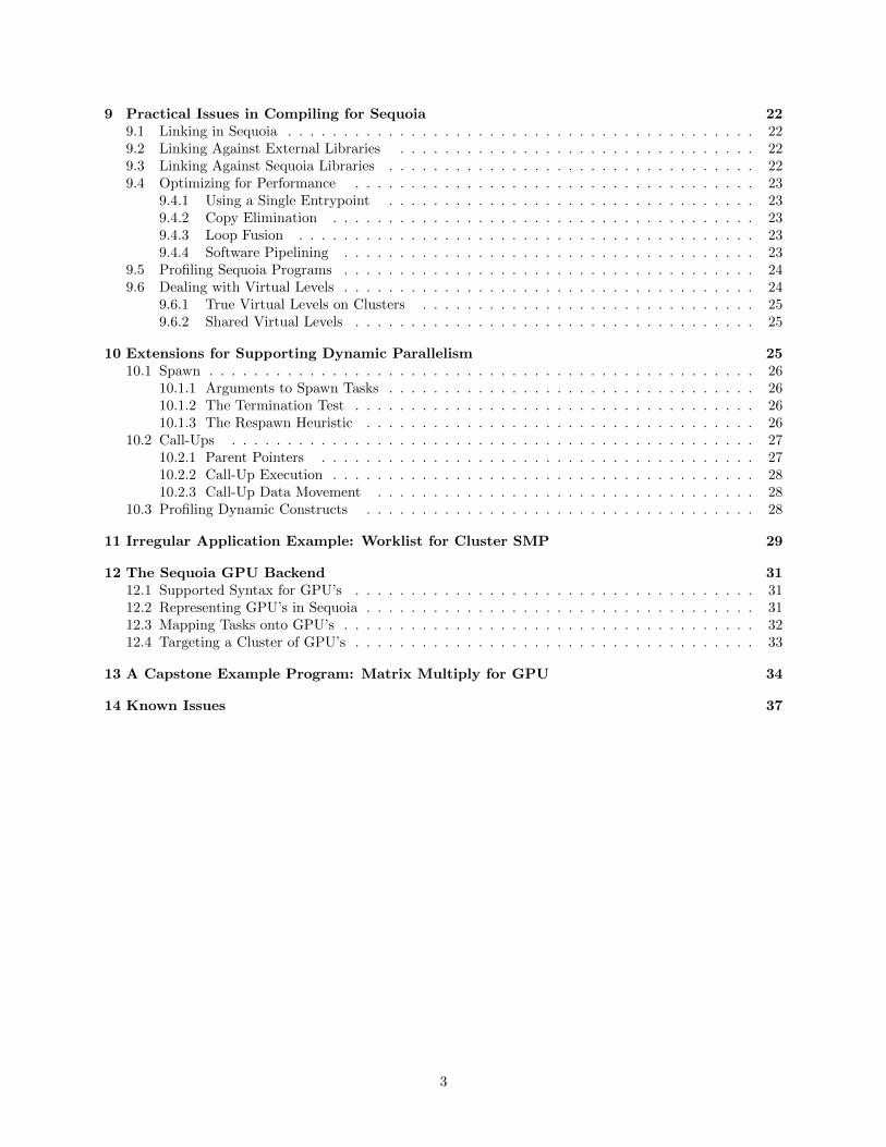
9 Practical Issues in Compiling for Sequoia 229.1 Linking in Sequoia . . . . . . . . . . . . . . . . . . . . . . . . . . . . . . . . . . . . . . . . . . 229.2 Linking Against External Libraries . . . . . . . . . . . . . . . . . . . . . . . . . . . . . . . . 229.3 Linking Against Sequoia Libraries . . . . . . . . . . . . . . . . . . . . . . . . . . . . . . . . . 229.4 Optimizing for Performance . . . . . . . . . . . . . . . . . . . . . . . . . . . . . . . . . . . . 23
9.4.1 Using a Single Entrypoint . . . . . . . . . . . . . . . . . . . . . . . . . . . . . . . . . 239.4.2 Copy Elimination . . . . . . . . . . . . . . . . . . . . . . . . . . . . . . . . . . . . . . 239.4.3 Loop Fusion . . . . . . . . . . . . . . . . . . . . . . . . . . . . . . . . . . . . . . . . . 239.4.4 Software Pipelining . . . . . . . . . . . . . . . . . . . . . . . . . . . . . . . . . . . . . 23
9.5 Profiling Sequoia Programs . . . . . . . . . . . . . . . . . . . . . . . . . . . . . . . . . . . . . 249.6 Dealing with Virtual Levels . . . . . . . . . . . . . . . . . . . . . . . . . . . . . . . . . . . . . 24
9.6.1 True Virtual Levels on Clusters . . . . . . . . . . . . . . . . . . . . . . . . . . . . . . 259.6.2 Shared Virtual Levels . . . . . . . . . . . . . . . . . . . . . . . . . . . . . . . . . . . . 25
10 Extensions for Supporting Dynamic Parallelism 2510.1 Spawn . . . . . . . . . . . . . . . . . . . . . . . . . . . . . . . . . . . . . . . . . . . . . . . . . 26
10.1.1 Arguments to Spawn Tasks . . . . . . . . . . . . . . . . . . . . . . . . . . . . . . . . . 2610.1.2 The Termination Test . . . . . . . . . . . . . . . . . . . . . . . . . . . . . . . . . . . . 2610.1.3 The Respawn Heuristic . . . . . . . . . . . . . . . . . . . . . . . . . . . . . . . . . . . 26
10.2 Call-Ups . . . . . . . . . . . . . . . . . . . . . . . . . . . . . . . . . . . . . . . . . . . . . . . 2710.2.1 Parent Pointers . . . . . . . . . . . . . . . . . . . . . . . . . . . . . . . . . . . . . . . 2710.2.2 Call-Up Execution . . . . . . . . . . . . . . . . . . . . . . . . . . . . . . . . . . . . . . 2810.2.3 Call-Up Data Movement . . . . . . . . . . . . . . . . . . . . . . . . . . . . . . . . . . 28
10.3 Profiling Dynamic Constructs . . . . . . . . . . . . . . . . . . . . . . . . . . . . . . . . . . . 28
11 Irregular Application Example: Worklist for Cluster SMP 29
12 The Sequoia GPU Backend 3112.1 Supported Syntax for GPU’s . . . . . . . . . . . . . . . . . . . . . . . . . . . . . . . . . . . . 3112.2 Representing GPU’s in Sequoia . . . . . . . . . . . . . . . . . . . . . . . . . . . . . . . . . . . 3112.3 Mapping Tasks onto GPU’s . . . . . . . . . . . . . . . . . . . . . . . . . . . . . . . . . . . . . 3212.4 Targeting a Cluster of GPU’s . . . . . . . . . . . . . . . . . . . . . . . . . . . . . . . . . . . . 33
13 A Capstone Example Program: Matrix Multiply for GPU 34
14 Known Issues 37
3
1 Introduction
Sequoia is a programming lanaguage for writing portable and efficient parallel programs. Sequoia is unusual inthat it exposes the underlying structure of the memory hierarchy to programmers, albeit in a manner abstractenough to ensure portability across a wide variety of contemporary machines. Sequoia is syntactically anextension to C++ and includes a number of C++ features, but the Sequoia-specific programming constructsresult in a programming model very different from C++. Sequoia provides language mechanisms to describethe movement of data through the memory hierarchy and provides mechanisms to localize computation anddata to particular levels of that hierarchy. This manual describes the high-level design of Sequoia and thetechnical details necessary to begin building programs using the Sequoia compiler.
Sequoia is also a work in progress—this is the first release. While we use the compiler ourselves everyday and have tested it fairly extensively, there are certain to be rough edges and outright bugs. Users whodon’t mind working with an experimental system will likely have a good experience; if you are looking for aproduction system this version of Sequoia is likely not for you. There is a core set of Sequoia features (whichwe will describe) that are well-tested and documented and should be sufficient to write significant Sequoiaprograms that work well. There are also more experimental features in the language that are included inthis release, but are currently not as complete as we would like (for example, some of these constructs do notcurrently work on all platforms, or only work with special annotations or other help from the programmer).We include these features in the current release because we have found them necessary for writing certainkinds of programs; if a feature is currently experimental or incomplete it is explicitly mentioned as such inthis manual, together with the limitations of the current implementation. Our intention is to remove theselimitations in future releases.
Feedback on the Sequoia implementation and this manual is welcome and can be sent to:
Note that you must join the sequoia-discuss google group in order to be able to post messages to the mailinglist. Anyone is welcome to join.
2 Sequoia Installation
Sequoia can be installed by downloading and then building its source code. There is currently no supportfor obtaining a pre-compiled binary.
2.1 Downloading Sequoia
The Sequoia source is in a .tar.gz file located at
http://www.stanford.edu/group/sequoia/sequoia.tar.gz
The remainder of this section assumes that the Sequoia compiler has been downloaded to a local directorynamed sqroot/.
2.2 Directory Structure
The Sequoia source tree is structured as follows:
• apps/ A collection of example applications, including extended versions of the examples shown inthis manual. Of particular note is the directory external/include which contains wrappers aroundstandard C headers which may be used by Sequoia programs.
• bin/ Contains the sq++ binary.
• doc/ Contains documentation, including the source for this manual.
• runtime/ Contains source code for runtime environments, which are described in detail in Section 6.
4

• src/ Contains the source code for the Sequoia compiler.
• test/ Contains a regressions test suite for the Sequoia compiler.
2.3 Compiler Dependencies
This section lists dependencies which must be satisfied to successfully build the Sequoia compiler.
2.3.1 Flex-Old
The Sequoia front end is based on the Elsa C++ front end [1], which depends on an older version of Flex writ-ten in C instead of C++. Consequently, the Sequoia compiler requires that Flex version 2.5.4a be installedprior to being built. In most Linux package managers, this version can be obtained by installing the flex-oldpackage. Alternatively the package can be obtained from http://packages.debian.org/sid/flex-old.
2.3.2 Xerces-C
The Sequoia compiler represents certain input files internally as XML. Consequently, the Sequoia compilerrequires that a recent version of Xerces be installed prior to being built. In most Linux package managers,Xerces can be obtained by installing the libxerces-c3.0 package. Alternately, we provide a pre-compileddll as part of this distribution (see sqroot/src/external/xercesc/). If an installed version of Xerces is tobe used, it is necessary to modify two files:
• sqroot/Makefile - Remove the statement -Lsrc/external/xerces/lib from the definition of LIBRARYand be sure to add the path to the installed version of Xerces to the LD LIBRARY PATH system variable
• sqroot/src/common/berkeley/src/elsa/Makefile.in - Modify the definition of the LIBXERCES vari-able to point to the correct installation of Xerces
2.4 Building the Compiler
Prior to building the Sequoia compiler the location of the xercesc library should be added to the LD LIBRARY PATHenvironment variable. For example, assuming that you are using the xerces dll that is distributed with Se-quoia and the Bash shell, you would type
$ export LD_LIBRARY_PATH=$LD_LIBRARY_PATH:sqroot/src/external/xercesc/lib
Having done so, the Sequoia compiler can be built by entering the sqroot directory and typing make. Toverify that the compilation succeeded, in the same directory, type make testbench.
2.5 Using the Compiler
Prior to using the Sequoia compiler, the following paths should be added to your environment. For example,assuming that you were using the Bash shell, you would type:
export PATH=$PATH:sqroot/bin # The location of the sq++ binary
export SQ_RT_DIR=sqroot/runtime # Paths that generated code will assume
export SQ_LD_DIR=sqroot/apps/external # to exist
2.5.1 The Compiler Workflow
Sequoia is a cross compiler: it generates appropriate source in a user-configurable target language. In general,the Sequoia compiler requires three types of input, which are described in further detail below: one or moresource (.sq) files, a machine (.m) file, and a mapping (.mp) file. The compiler can be invoked by specifyingthe names of those files and several optional flags:
$ sq++ foo.sq bar.sq machine.m mapping.mp -d -O
5
Using the -d flag instructs the compiler to produce debugging output in a directory named debug/. Usingthe -O flag instructs the compiler to turn on optimizations.
When the Sequoia compiler runs successfully, it produces a directory named out. In addition to containingsource code in the target language, the directory also contains a Makefile. The contents of the directory canbe built by entering out/ and typing make. The resulting binary will be named sq.out.
2.5.2 Migrating Generated Source to Target Machines
In addition to being compiled locally, the out directory can also be exported and compiled on a target ma-chine. The only requirement for doing so is that the directories sqroot/runtime and sqroot/apps/external
exist on the target machine and the environment variables described above be defined appropriately.
3 Programming in Sequoia
3.1 Abstract Machine Model
Sequoia’s abstract machine model is very different from the abstract machine model of C++ or any conven-tional sequential language. C++’s abstract machine model is characterized by a single memory space, whereevery program variable has an address in that space. It assumes the existence of a single processor that canrandomly access every memory address using fine-grained, byte-granularity, pointer dereferencing.
The primary distinguishing feature of Sequoia’s abstract machine model is that it contains multipleindependent memory spaces that are exposed to the programmer. The Sequoia abstract machine modelconsists of a tree of memories, where each level of the tree corresponds to a level of the memory hierarchyof the machine. Memories closer to the leaf level of the tree are assumed to be both smaller and faster thanmemories in the levels near the root. For example, a degenerate tree is the memory hierarchy of a standarduniprocessor machine, consisting of the cache (or multiple levels of cache) and DRAM, with the DRAM atthe root and the L1 cache the sole leaf. More complex hieararchies in parallel machines, such as clusters orshared-memory multiprocessors, form non-trivial trees.
In Sequoia data can be transferred between a memory and its children, for example via asynchronousbulk transfers such as DMA commands or cache prefetches. The machine model also includes a processingelement for each distinct memory in the tree.1 Processing elements closer to the leaves of the tree areassumed to be faster than processing elements in the levels above them. A processing element can onlyoperate directly on data stored in its associated memory. Programming such a machine requires transferringdata from the large, slow outer memory levels into the small, fast local memory levels at or near the leaveswhich the high-performance processing elements can access.
3.2 Programming Model
The Sequoia abstract machine model is a tree of memories, each with its own processor. The programmingmodel is a tree of tasks, with each task mapped to one memory in the tree-shaped memory hierarchy. Thus,Sequoia encourages writing divide-and-conquer style algorithms, where a problem is divided into smallersubproblems that can be solved in parallel and independently, including potentially recursively subdividingthe subproblems further.
Tasks are isolated from each other and, except for invoking other tasks, have no mechanism for commu-nicating with other tasks. Tasks execute entirely within one level of the memory hierarchy; all data andcomputation for the task is located in that memory for the duration of the task’s lifetime. When a parenttask invokes a child task, the child need not run in the same memory level as the parent. A typical Sequoiatask breaks its computation up into smaller subproblems, each of which is handled in parallel by a subtaskrunning in some smaller/faster memory level. To summarize, tasks are the unit of computation and localityin Sequoia, and task calls are communication, where data is moved from one place in the machine to another.
The tasks the programmer writes are abstract; they do not mention specific memory levels in a concretemachine or the size of the memory. When a Sequoia program is compiled for a particular machine, the details
1This is different from the model in the original Sequoia paper, which effectively assumed that there was a processor onlyat each leaf of the memory hierarchy.
6

of the machine’s specific memory hierarchy are instantiated by a mapping in which the programmer stateshow each task is specialized to the machine. The mapping of a task has two parts. First, the task’s data(arguments and local variables) is assigned to a specific level of the memory hierarchy. The memory levelhas a specific size and the task’s data must fit within that size; the mapping also specifies whether this sizeis checked statically by the compiler or at run-time when the task is called. Second, the task’s computationis assigned to a specific processor in the machine that has access to the level of the hierarchy where thetask’s data will reside. Mappings of the same program to different machines are often very different. ASequoia program does not itself mention the machine-specific details in a mapping and is therefore machineindependent and relatively easy to port; in our experience writing a mapping for an existing Sequoia programto target a new machine is usually straightforward.
If a task whose data is mapped to a memory in level i of the machine calls a subtask whose data ismapped to level i− 1, when the task at level i makes its subtask call the arguments will be physically copiedfrom level i to level i− 1; similarly, when the subtask completes data returned from level i− 1 is copied backto the calling task in level i. Movement of data in a task call or return is the only form of communicationin Sequoia.
The Sequoia compiler and runtime automatically use the appropriate hardware or software mechanismsto implement the data transfers. In fact, this is one of the major benefits of programming in Sequoia, as theprogrammer only uses one way of communicating data and the compiler generates the code that uses theappropriate API for moving data between the two concrete levels of the memory hierarchy, whether that bevia MPI calls, DMAs, explicit loads and stores, etc. The compiler also removes as many copies as possiblevia program optimizations, including copies introduced by copying arguments to tasks. It is also possible tomanually (and unsafely) turn off some copying via specifications in the mapping file.
7

4 A Motivating Example Program: SAXPY for SMP
In this section we introduce Sequoia using a SAXPY kernel, a simple, but complete, Sequoia program. SAXPYis a single precision floating point multiply-add operation on two vectors ( Single a ∗ X + Y ). Compilingthis or any Sequoia program involves three separate input files:
• Listing 1 gives the machine independent source code. There is a main method that initializes twovectors of size N with some random values. These two vectors are then passed as arguments to theSAXPY kernel. There are two different variants of the SAXPY kernel: one is an inner task (a task thatcalls subtasks) and the other is a leaf task (a task with no subtasks). Note that the call to the SAXPY
kernel in the the main function does not specify which of the two instances of the SAXPY kernel isinvoked.
• Listing 3 gives the mapping file for SAXPY. Among other things, the mapping specifies whether to callthe inner or leaf task variant. We discuss how to specify task variants for task call sites in a mappingfile in Section 8.
• Listing 2 is a machine description, which specifies the properties of the target machine. In this casewe are compiling for a two-level SMP machine with two processors. We discuss the details of machinedescriptions in Section 7.
1 void task<inner> saxpy ( in f loat x [N] , inout f loat y [N] , in f loat a ) ;2 void task<l e a f > saxpy ( in f loat x [N] , inout f loat y [N] , in f loat a ) ;34 int main ( )5 {6 const unsigned int N = 16 ∗ 1024 ∗ 1024 ;78 f loat ∗ x = new float [N ] ;9 f loat ∗ y = new float [N ] ;
10 for ( unsigned int i = 0 ; i < N; i++ )11 {12 x [ i ] = static cast<f loat>( i % 99) ;13 y [ i ] = 10 .0 + static cast<f loat>( i % 99) ;14 }15 f loat a = 2 . 0 ;1617 saxpy (x , y1 , a ) ;1819 delete [ ] x ;20 delete [ ] y ;2122 return 0 ;23 }24 void task<inner> saxpy ( in f loat x [N] , inout f loat y [N] , in f loat a )25 {26 tunable b l o ckS i z e ;27 mappar ( int i=0 : N/ b lo ckS i z e )28 saxpy ( x [ i ∗ b lo ckS i z e ; b l o ckS i z e ] , y [ i ∗ b lo ckS i z e ; b l o ckS i z e ] , a ) ;29 }30 void task<l e a f > saxpy ( in f loat x [N] , inout f loat y [N] , in f loat a )31 {32 for ( int i =0; i < N; i++ )33 y [ i ] += a ∗ x [ i ] ;34 }
Listing 1: SAXPY source file
1 32 b i t machine smp22 {3 managed shared smp l e v e l 1(256 Mb @ 128 b) : 2 c h i l d r e n ;4 smp l e v e l 0(256 Mb @ 128 b) ;5 }
Listing 2: SAXPY machine file
8

1 in s t ance saxpy i ( l e v e l 1) inner2 {3 ent rypo int main [ 0 ] ;4 tunable b l o ckS i z e = 2ˆ24 / 2 ;5 data ( )6 {7 array x ( ) { e lements = 2ˆ24 ; }8 array y ( ) { e lements = 2ˆ24 ; }9 }
10 c o n t r o l ( l e v e l 0)11 {12 loop i ( ) { spmd { f u l l r a n g e = 0 , 2 ; ways = 2 ; i t e r b l k = 1 ; } }13 c a l l s i t e saxpy ( ) { t a r g e t l ( ) {} }14 }15 }16 in s t ance saxpy l ( l e v e l 0) l e a f { }
Listing 3: SAXPY mapping file
5 Sequoia Language Constructs
Sequoia is based on C++ and the syntax has been chosen to be consistent with C++ conventions. Sequoiadoes not support all of C++; this section discusses Sequoia’s language constructs.
5.1 Base Language Features
This section discusses the core sequential language features of Sequoia.
5.1.1 Classes and Objects
Sequoia supports C++ classes. Tasks may be members of classes.
5.1.2 Templates
Sequoia supports a subset of C++ templates, enough to write generic Sequoia libraries but not so much thatthe implementation effort is overwhelming. Non-nested templates work. Templated tasks also work. Nestedtemplates are not supported.
5.1.3 Memory Management
Sequoia supports dynamic memory allocation within a single memory level. That is, a task may dynamicallyallocate objects and build linked data structures. However, the language is constrained so that there arenever pointers between memory levels (see the restrictions on task parameter passing in Section 5.2). Thus,every task has its own local heap in which it can allocate and deallocate objects, and every task heap isisolated from every other heap. Sequoia provides the C++ and C routines new/delete and malloc/free.
An important property of a task is the amount of memory it will consume; the fastest memory levels onmany machines are small and knowing that task data will fit can be crucial to developing a working andhigh-performance program. As mentioned above, the Sequoia compiler attempts to compute the size of taskdata statically, but in the presence of dynamic memory allocation this may not be possible, in which casethe programmer must supply a bound on the size of task data in the mapping file.
When dynamically allocating memory in tasks, a good rule of thumb is that all data that is allocatedwithin a task should also be reclaimed within that same task. This protects against memory leaks as thereis no way to refer to a piece of created data after a task has finished.
9

5.1.4 Unsupported Features of C++
There are some features of C++ that are not supported.
• Global variables have no meaning in Sequoia, as every value is local to some task.
• Type unions are not currently part of the language.
• Virtual tasks are not supported, but Sequoia does support ordinary virtual functions. Disallowingvirtual tasks makes the task-call hierarchy completely static, enabling many optimizations that wouldbe much more difficult to implement otherwise.
• Multiple inheritance is not supported.
• extern functions are not supported. The compiler currently has no linker, therefore all functions mustbe in scope when compiling a Sequoia file. For more information see Section 9.1.
5.2 Tasks and Task Argument Type Qualifiers
A task is a function marked with the task keyword. Tasks are restricted in that they the can only modifydata local to the task; externally, a task is a pure function. Task arguments are passed call-by-value-result,which means that the arguments are copied to the task’s formal parameters the task’s return values arecopied back. Sequoia currently distinguishes between inner and leaf tasks. Inner tasks are used to breakup the work that is to be done at lower levels of the machine; inner tasks can call subtasks. Leaf tasks arecompute kernels that carry out the bulk computation of the algorithm; leaf tasks may not invoke subtasks.Below are examples of an inner task and a leaf task declarations for matrix-matrix multiplication:
task<inner> void matrixmult(in float a[M][P], in float b[P][N], out float c[M][N]);
task<leaf> void matrixmult(in float a[M][P], in float b[P][N], out float c[M][N]);
The inner task is used to recursively divide up the matrices a, b, and c. These three matrices, together withthe variables M, P, and N, which give the sizes of the arrays, are the arguments to the tasks. The argumentsare labeled in (read only, only copied to the task) or out (write only, only copied back from the task’sfinal state on exit to the position of the argument array in the caller). There is also an inout keyword forarguments that are both read and written (not used in this example). Below are possible implementationsof both the inner and leaf tasks:
task<inner> void matrixmult(in float a[M][P], in float b[P][N], out float c[M][N])
{
tunable mBlock;
tunable pBlock;
tunable nBlock;
mappar ( int i = 0 : M/mBlock, int j = 0 : N/nBlock )
mapseq ( int k = 0 : P/pBlock )
matrixmult(a[i*mBlock;mBlock][k*pBlock;pBlock],
b[k*pBlock;pBlock][j*nBlock;nBlock],
c[i*mBlock;mBlock][j*nBlock;nBlock]);
}
task<leaf> void matrixmult(in float a[M][P], in float b[P][N], out float c[M][N])
{
for ( unsigned int i = 0; i < M; i++ )
for ( unsigned int j = 0; j < N; j++ )
10
{
c[i][j] = 0.0;
for ( unsigned int k = 0; k < P; k++ )
c[i][j] += a[i][k] * b[k][j];
}
}
Note that in the Sequoia program tasks do not yet have information about the number of levels in thememory hierarchy, in fact there is no machine dependent information specified in the task definitions at all.In sections 7 and 8 we will describe the machine and mapping files which take the abstract algorithm definedin terms of tasks and instantiate it for a specific architecture.
5.3 Tunable Variables
The variables mBlock, pBlock, and nBlock are tunables. Tunables are intended to be used for values thatare compile-time constants that vary from machine to machine; for example, in the matrix multiply examplethe three tunables correspond to the block sizes chosen for a particular level of the memory hierarchy on thetarget machine. The values of tunables are set in a mapping file, which allows different constants to be usedfor different machines. Note also that when tasks are recursive there may be more than one instance of thetask at runtime that execute at different levels of the memory hierarchy. Mapping files also allow differenttunables to be specified for different instances of the same task on a single machine.
Notice that the inner task is recursive. Each recursive call will traverse one level deeper in the memoryhierarchy further dividing up the work to be done by the lowest level. The leaf task is the base case of therecursion. The leaf task will run on the lowest level of the machine (where in most modern architecturesthe smallest memory and most power processing live) and will carry out the actual computation, in thiscase matrix matrix multiplication. The mappar and mapseq are parallel and sequential looping constructsrespectively and will be described in more detail in section 5.4.
Indexing in a leaf task is relative to that task’s sub-problem size. If the original matrices were 100x100and one inner task is instantiated (see section on mapping) with mBlock = pBlock = nBlock = 50 thenin the leaf task above the parameters will have values M = 50N = 50P = 50. Therefore the leaf taskwill compute the product of two 50x50 matrices and return the result as a 50x50 sub-matrix of the originalmatrix c. Even though a leaf task may be computing the (2,2) sub-matrix of c the indexes in the leaf taskwill still start at zero. That is, a leaf task does not need to know where in the over all data its data islocated, Sequoia takes care of managing it. The actual syntax of array block is cover in section 5.6.
5.4 Parallelism Constructs
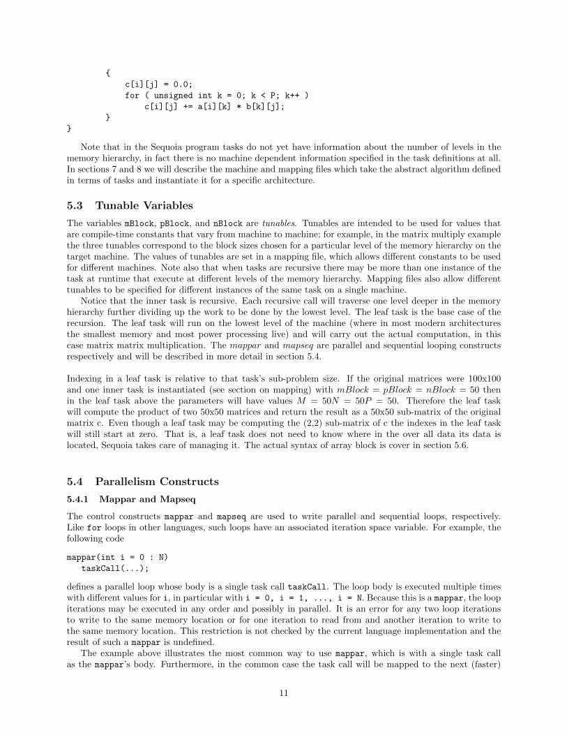
5.4.1 Mappar and Mapseq
The control constructs mappar and mapseq are used to write parallel and sequential loops, respectively.Like for loops in other languages, such loops have an associated iteration space variable. For example, thefollowing code
mappar(int i = 0 : N)
taskCall(...);
defines a parallel loop whose body is a single task call taskCall. The loop body is executed multiple timeswith different values for i, in particular with i = 0, i = 1, ..., i = N. Because this is a mappar, the loopiterations may be executed in any order and possibly in parallel. It is an error for any two loop iterationsto write to the same memory location or for one iteration to read from and another iteration to write tothe same memory location. This restriction is not checked by the current language implementation and theresult of such a mappar is undefined.
The example above illustrates the most common way to use mappar, which is with a single task callas the mappar’s body. Furthermore, in the common case the task call will be mapped to the next (faster)
11

level of the memory hieratchy below the level of the mappar itself. While a single task call that runs at thechildren of the current level is the usual idiom, mappars may have arbitrary code in their body and mayalso be mapped to the parent instead of child level. Note, however, that only the task calls are executed inparallel; any other code is executed as part of the current task.
A mapseq specifies a sequential loop: the instances of the mapseq body must be executed in the ordergiven by the programmer. There are no restrictions on what the body of a mapseq can read or write (becausethe execution order of iterations is fixed, no restrictions are needed). A mapseq should be used wheneverthere are read/write or write/write dependencies between the iterations of the loop. Note that even thoughthe iterations may be dependent, the compiler may still be able to extract some parallelism through softwarepipelining of the mapseq body across multiple iterations.
Now consider a simple version of matrix multiply that uses a combination of mappar and mapseq:
mappar( int i = 0 : M/mBlock )
mappar( int j = 0 : N/nBlock )
mapseq( int k = 0 : P/pBlock )
matrixmult( ... );
In this example we have a three dimensional iteration space: each task is associated with a triple (i, j, k).The important thing to note is that by nesting the control constructs, and specifically the mapseq, in aparticular order we specify a certain execution order of the iteration space. In this case, we are sayingthat all tasks sharing the same (i, j) must be executed in order of increasing k. However, any two taskswith distinct (i, j) may executed in parallel. It is important to note that by placing the mapseq in theinnermost construct, we are expressing as much parallelism as possible for the compiler to take advantageof when performing scheduling. If we were to rearrange the loops and place the mapseq on the outside, theanswer would be the same, but there would be significantly reduced parallelism as all combinations of (i, j)associated with a given k would have to be executed before the next set of (i, j) could be executed.
A control construct may declare multiple iteration space variables. The following code is equivalent tothe previous example:
mappar( int i = 0 : M/mBlock , int j = 0 : N/nBlock )
mapseq( int k = 0 : P/pBlock )
matrixmult( ... );
While iteration space variables may not be assigned, they are otherwise just like any other variable andcan be used anywhere in the body of the control construct that declares them.
5.4.2 Mapreduce
Another control construct provided by Sequoia is mapreduce, which is designed for processing in parallelsub-problems that will be combined into a final answer via an associative reduction. In the following versionof the matrix-matrix multiplication example the mapseq has been replaced by a mapreduce:
mappar( int i = 0 : M/mBlock , int j = 0 : N/nBlock )
mapreduce( int k = 0 : P/pBlock )
matrixmult( ... , reducearg<c,matrixadd>, ... );
The mapreduce syntax is identical to mappar. The task call, however, takes an additional reductionargument description, denoted by the keyword reducearg followed by the name of the array to be reducedand the name of a leaf task that implements the combining operation. In this example the k loop iteratesover the inner P dimension of the matrices and so iterates over dependent computations. That is, the resultsof the matrix-matrix products computed as sub-problems along the inner dimension of the a and b matricesmust be added together to form a final block of the matrix c. This example computes these dependentsub-problems in parallel and then uses the combiner leaf task matrixadd to reduce the results of each sub-problem into a single block of the c matrix. The leaf task matrixadd must take as arguments two arrays;the first array must be an in parameter and the second must be an inout parameter. At run time themapreduce consumes the results of the subproblems in a combining tree where the leaf task is repeatedly
12
run on two arrays, storing the result in the second array argument. The final result is stored back at theparent memroy level.
The reducearg need not be an entire array. In the example the reducearg shown above reduces the entirematrix c into the final matrix c. The reduction also can be done on independent sub-blocks of the matrix c
by using array blocking to specify sub-blocks of the matrix. Array blocking is described in Section 5.6.
5.5 Task Calls
There are a few rules of thumb for getting the best performance and portability from tasks:
• The best performance is achieved if only task calls are placed in the parallel control constructs.
• For maximum portability task calls should be generic: they should not name which variant of the taskis to be called. The variant is specified in the mapping file.
• Tasks should be designed to break big problems into smaller problems recursively if that is appropriateto the problem being solved. Thus the inner task variant will typically call the same task (with novariant specified). This recursive structure will be mapped by the compiler on to the memory hierarchyof the machine, with as many instances of the inner task as needed to cover the number of levels ofthe target machine.
Note that tasks can only be called after they have been declared; forward declarations can be used ifnecessary.
5.5.1 Entrypoints and Callsites
If a task is called from outside of Sequoia (for example calling a task from main() in a C program), thatinstance of the task must be labelled with an entrypoint. The entrypoint construct is described in Section 8.3.When a task calls another task an entrypoint is not used, instead one defines a callsite inside the controlblock of the instance of the calling task (see Section 8.2).
5.6 Array Blocking
Array blocking allows the programmer to partition an array into smaller arrays. In combination with oneof the Sequoia control constructs a programmer can pass the different parts of the array to different taskinstances. Consider again the matrix multiplication example:
// a, b, and c are two dimensional arrays
mappar( int i = 0 : M/mBlock , int j = 0 : N/nBlock )
mapseq( int k = 0 : P/pBlock )
matrixmult(a[i*mBlock;mBlock][k*pBlock;pBlock],
b[k*pBlock;pBlock][j*nBlock;nBlock],
c[i*mBlock;mBlock][j*nBlock;nBlock]);
Each task is passed a portion of each of arrays a, b, and c. The task either recursively subdivides itsportions of the arrays in further task calls (for an inner task call) or performs an actual matrix multiplication(in a leaf task call). Notice that each dimension of the array has its own pair of brackets [...]. Arrays mustalways be fully indexed, meaning that a n-dimensional array must always be used with all n dimensions.Array blocking has two arguments per dimension. The first argument describes the index where the blockbegins, and the second argument specifies the number of elements. For example, for the a matrix in the x
dimension, the partition passed to the i-th task consists of mBlock elements beginning at index i ∗ mBlock.For the y dimension pBlock elements are taken beginning at k ∗ pBlock.
Note that many different parallel tasks (all with different values of j) are passed the same sub-array of a.Because a is declared to be an in (read-only) parameter it presents no problem for multiple tasks to sharethe same portion of a. However, any argument annotated out or inout can only be passed to a single paralleltask as it is undefined what occurs if multiple parallel tasks attempt to write the same output location. Asdiscussed previously, this requirement is not currently checked by the Sequoia compiler.
13

5.6.1 The Copy Operator
The copy operator is a special built-in function available only in inner tasks; copy is a reserved keyword inSequoia. The copy operator can be used in two distinct ways:
• A array block, as described in Section 5.6, can be copied to another array block with the same numberof elements in each dimension. For example,
void task<inner> copyExample1(in int B[W][X], inout int A[Y][Z])
{
copy(A[2:5;3][3:9;5], B[1:4;3][1:6;5]);
}
This example copies a 3x5 block from array B beginning at (1,1) into array A beginning at index (2,3).The syntax is redundant in that we must specify both the start (inclusive) and ending (exclusive)points in each dimension as well as the size to transfer, however this redunancy makes it possible forthe compiler to verify correctness. Notice also that these are contiguous blocks of memory as arrayblocks always use stride 1.
In the case where we want to move an entire array, we do not use the blocking syntax for that array.For example,
void task<inner> copyExample2(in int B[W][X], inout int A[Y][Z])
{
copy(A[0:5;5][1:9;8], B);
}
Here we assume that B has size 5x8 and that we are copying the entire array B into A starting at (0,1).Note that reversing the arguments expresses copying a portion of A into all of B.
• The copy operator also supports arbitrary gather and scatter operations, but only for one dimensionalarrays. We use an indexing array as an argument in the blocking syntax to specify the gather orscatter. An example gather is
// Idx = {3,8,5,11,12,11,16}
void task<inner> copyExample3(in int B[X], inout int A[Y], in int Idx[Z])
{
copy(A[2:9;7], B[Idx]);
}
The indexing array Idx provides the indices of the source locations in B. Note that the number ofelements in Idx is the same as the number of elements copied to A. Sequoia also supports scatters;reversing the arguments in this example would scatter the contiguous elements of A into the elementsof B given by Idx. Sequoia does not support an all-to-all copy scheme; only one of the two argumentscan use an indexing array.
Whichever version of the copy operator is used, the two array blocks must represent disjoint sets oflocations.
6 Target Machines
The Sequoia compiler is designed to target a wide array of machines. A key aspect of this portability isthat the compiler generates code for a generic runtime interface [2]. In this section we explain the runtimeinterface and discuss the various runtimes provided with this version of the compiler.
14
6.1 The Portable Runtime Interface
The runtime interface presents a single target for the Sequoia compiler, eliminating the need for the compilerto maintain a separate backend for every target architecture. Our experience is that maintaining a runtimeimplementation is significantly easier than maintaining a compiler backend; the runtime interface isolatesthe compiler from the details of particular architectures.
Each Sequoia runtime implements an interface for two adjacent levels of the memory hierarchy. Theruntime interface provides methods for the parent level to allocate memory in the child level, copy datato and from the child level, and launch tasks on child processors. Similarly, there are methods that thechildren can invoke to interact with the parent. An important feature of Sequoia runtimes is that they arecomposable: a runtime for a machine with more than two levels of memory hierarchy is built by composingindividual runtimes for each pair of adjacent levels. For example, the Sequoia compiler can target an MPIcluster where each node has a multicore processor and several GPU’s by composing the MPI, CMP, andCUDA runtimes. In general all of the runtimes compose, however certain runtimes currently can be usedonly at either the top of the machine or at the bottom. As an example, the MPI cluster should always bethe top-level runtime whenever it is used 2 Also, the GPU runtime must always be the bottom-most runtimeas it is currently impossible to call to another machine from within a thread on a GPU.
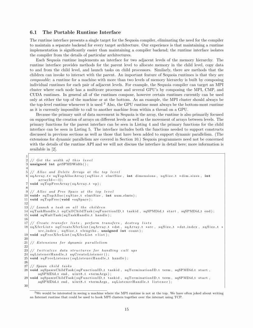
Because the primary unit of data movement in Sequoia is the array, the runtime is also primarily focusedon supporting the creation of arrays on different levels as well as the movement of arrays between levels. Theprimary functions for the parent interface can be seen in Listing 4 and the primary functions for the childinterface can be seen in Listing 5. The interface includes both the functions needed to support constructsdiscussed in previous sections as well as those that have been added to support dynamic parallelism. (Theextensions for dynamic parallelism are covered in Section 10.) Sequoia programmers need not be concernedwith the details of the runtime API and we will not discuss the interface in detail here; more information isavailable in [2].
12 // Get the width o f t h i s l e v e l3 unsigned int getSPMDWidth ( ) ;45 // Al loc and Dele te Arrays at the top l e v e l6 sqArray t ∗ sqTopAllocArray ( s q S i z e t e lmtSize , int dimensions , s q S i z e t ∗ d im s i ze s , int
arrayId=−1) ;7 void sqTopFreeArray ( sqArray t ∗p) ;89 // Al loc and Free Space at the top l e v e l
10 void∗ sqTopAlloc ( s q S i z e t e lmtSize , int num elmts ) ;11 void sqTopFree (void ∗ sqSpace ) ;1213 // Launch a ta sk on a l l the ch i l d r en14 sqTaskHandle t sqCal lChi ldTask ( sqFunct ionID t task id , sqSPMDid t s ta r t , sqSPMDid t end ) ;15 void sqWaitTask ( sqTaskHandle t handle ) ;1617 // Create t r an s f e r l i s t s , perform t rans f e r s , de s t roy l i s t s18 sqXf e rL i s t ∗ sqCreateXfe rL i s t ( sqArray t ∗dst , sqArray t ∗ src , s q S i z e t ∗ dst index , s q S i z e t ∗
s r c index , s q S i z e t ∗ l engths , unsigned int count ) ;19 void sqFreeXfe rL i s t ( sqXf e rL i s t ∗ l i s t ) ;2021 // Extensions f o r dynamic p a r a l l e l i sm2223 // I n i t i a l i z e data s t r u c t u r e s f o r hand l ing c a l l ups24 sqL i s t ene rHand l e t sqCrea t eL i s t ene r ( ) ;25 void sqFre eL i s t ene r ( sqL i s t ene rHand l e t handle ) ;2627 // Spawn c h i l d t a s k s28 void sqSpawnChildTask ( sqFunct ionID t task id , sqTerminat ionID t term , sqSPMDid t s ta r t ,
sqSPMDid t end , u i n t 8 t ∗ termArgs ) ;29 void sqSpawnChildTask ( sqFunct ionID t task id , sqTerminat ionID t term , sqSPMDid t s ta r t ,
sqSPMDid t end , u i n t 8 t ∗ termArgs , sqL i s t ene rHand l e t l i s t e n e r ) ;30
2We would be interested in seeing a machine where the MPI runtime is not at the top. We have often joked about writingan Internet runtime that could be used to hook MPI clusters together over the internet using TCP.
15
31 // A d i f f e r e n t wait f o r hand l ing mappars t ha t may contain c a l l ups32 void sqWaitTask ( sqTaskHandle t handle , sqL i s t ene rHand l e t l i s t e n e r ) ;3334 // Pu l l data up to the parent in the case o f c a l l ups35 sqXferHandle t sqParentPul l ( s qX f e rL i s t ∗ l i s t , sqSPMDid t ch i ldID ) ;
Listing 4: Parent Runtime Functions
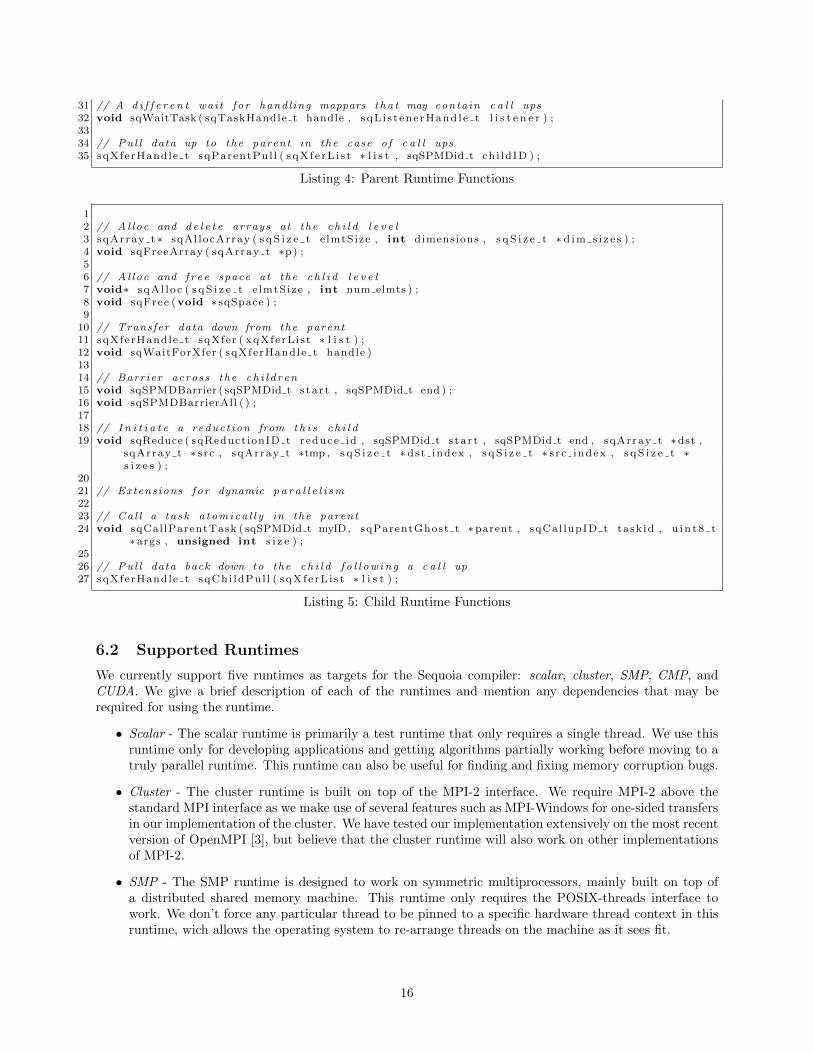
12 // Al loc and d e l e t e arrays at the c h i l d l e v e l3 sqArray t ∗ sqAl locArray ( s q S i z e t e lmtSize , int dimensions , s q S i z e t ∗ d i m s i z e s ) ;4 void sqFreeArray ( sqArray t ∗p) ;56 // Al loc and f r e e space at the c h l i d l e v e l7 void∗ sqAl loc ( s q S i z e t e lmtSize , int num elmts ) ;8 void sqFree (void ∗ sqSpace ) ;9
10 // Transfer data down from the parent11 sqXferHandle t sqXfer ( xqXferL i s t ∗ l i s t ) ;12 void sqWaitForXfer ( sqXferHandle t handle )1314 // Barr ier across the ch i l d r en15 void sqSPMDBarrier ( sqSPMDid t s ta r t , sqSPMDid t end ) ;16 void sqSPMDBarrierAll ( ) ;1718 // I n i t i a t e a reduc t ion from t h i s c h i l d19 void sqReduce ( sqReduct ionID t reduce id , sqSPMDid t s ta r t , sqSPMDid t end , sqArray t ∗dst ,
sqArray t ∗ src , sqArray t ∗tmp , s q S i z e t ∗ dst index , s q S i z e t ∗ s r c index , s q S i z e t ∗s i z e s ) ;
2021 // Extensions f o r dynamic p a r a l l e l i sm2223 // Ca l l a t a s k a tomica l l y in the parent24 void sqCal lParentTask ( sqSPMDid t myID, sqParentGhost t ∗parent , sqCal lupID t task id , u i n t 8 t
∗ args , unsigned int s i z e ) ;2526 // Pu l l data back down to the c h i l d f o l l ow i n g a c a l l up27 sqXferHandle t sqChi ldPul l ( s qX f e rL i s t ∗ l i s t ) ;
Listing 5: Child Runtime Functions
6.2 Supported Runtimes
We currently support five runtimes as targets for the Sequoia compiler: scalar, cluster, SMP, CMP, andCUDA. We give a brief description of each of the runtimes and mention any dependencies that may berequired for using the runtime.
• Scalar - The scalar runtime is primarily a test runtime that only requires a single thread. We use thisruntime only for developing applications and getting algorithms partially working before moving to atruly parallel runtime. This runtime can also be useful for finding and fixing memory corruption bugs.
• Cluster - The cluster runtime is built on top of the MPI-2 interface. We require MPI-2 above thestandard MPI interface as we make use of several features such as MPI-Windows for one-sided transfersin our implementation of the cluster. We have tested our implementation extensively on the most recentversion of OpenMPI [3], but believe that the cluster runtime will also work on other implementationsof MPI-2.
• SMP - The SMP runtime is designed to work on symmetric multiprocessors, mainly built on top ofa distributed shared memory machine. This runtime only requires the POSIX-threads interface towork. We don’t force any particular thread to be pinned to a specific hardware thread context in thisruntime, wich allows the operating system to re-arrange threads on the machine as it sees fit.
16

• CMP - The CMP runtime is designed to work in a similar manner to the SMP runtime, but it assumesthat we want to pin a thread to a given hardware thread context. We use the p-threads affinityscheduling interface to attempt to pin certain threads to a given hardware context. This allows theCMP runtime to guarantee reuse of data left in caches. The CMP runtime is primarily used only forworking with CMP’s where cache locality is very important.
• CUDA GPU - This runtime supports a single CUDA GPU. This runtime is coupled with a specialbackend for the generating CUDA-specific code. While in principle we could use a pure dynamicruntime, threads in CUDA often do so little computation that the overhead of implementing theruntime interface as full function calls at runtime can be prohibitive and we gain a great deal bymoving some of that work to compile time. Also, as of the CUDA 2.3, when we first implemented theCUDA backend, CUDA was not expressive enough to fully support all of the functions required forour runtime interface. We require at least CUDA 2.3 and the runtime has been tested through CUDA3.0 [4].3 The CUDA runtime and backend are discussed further in Section 12.
• CUDA CMP - This runtime supports multiple GPU’s. Currently this runtime must be the top-levelruntime in a given process, which means that the only runtime that could be placed on top of thisruntime is the cluster. The cluster will generate a new MPI process for each of its children, andtherefore the threads will be managing devices on different nodes (assuming only one MPI process pernode). It should be noted that if there is only a single GPU available then the single GPU runtime ismore efficient as it does not require inter-thread communication using locks. There is more informationabout the CMP-GPU runtime in Section 12.4.
7 Machine File Syntax
A machine file specifies a concrete implementation of the abstract Sequoia memory hierarchy. Every validSequoia program must contain exactly one non-empty machine file.
7.1 Machine Statements
A machine file consists of a single machine statement of the form
N bit machine ID { ... }
where N is the size of addressable memory common to all levels of the hierarchy, and ID is the name of themachine. The value of N may be either 32 or 64, and ID may be an arbitrary C-style identifier.
7.2 Level Statements
The body of a machine statement consists of one or more level statements, each describing a level of thememory hierarchy. Within a level of the memory hierarchy, nodes are assumed to be homogeneous; regardlessof the width of a memory level, only a single level statement is required. The form of a level statement is
managed shared virtual T level N (M @ W) : C children;
where managed, shared, and virtual are optional modifiers with the following meanings:
• managed: Memory at this level is OS-managed. If present, this flag indicates that the dynamic alloca-tion and deallocation of memory at a particular level is backed by a virtual memory system.
• shared: Memory at this level is shared. If present, this flag indicates that the processing elements ata particular level may communicate through shared memory.
3With the release of CUDA Fermi we have not attempted implementing the runtime interface in the richer GPU languagesupported by Fermi. This might be an interesting experiment, but we worry about some of the overhead associated with moreexpensive language features required for our runtime interface, such as virtual function dispatch.
17
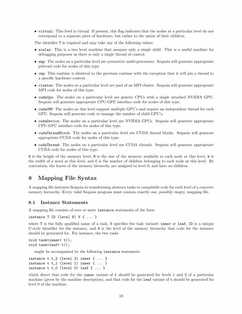
• virtual: This level is virtual. If present, this flag indicates that the nodes at a particular level do notcorrespond to a separate piece of hardware, but rather to the union of their children.
The identifier T is required and may take any of the following values:
• scalar: This is a two level machine that assumes only a single child. This is a useful machine fordebugging purposes as there is only a single thread of control.
• smp: The nodes on a particular level are symmetric multi-processors. Sequoia will generate appropriatepthread code for nodes of this type.
• cmp: This runtime is identical to the previous runtime with the exception that it will pin a thread toa specific hardware context.
• cluster: The nodes on a particular level are part of an MPI cluster. Sequoia will generate appropriateMPI code for nodes of this type.
• cudaCpu: The nodes on a particular level are generic CPUs with a single attached NVIDIA GPU.Sequoia will generate appropriate CPU-GPU interface code for nodes of this type.
• cudaCMP: The nodes on this level support multiple GPU’s and require an independent thread for eachGPU. Sequoia will generate code to manage the number of child GPU’s.
• cudaDevice: The nodes on a particular level are NVIDIA GPUs. Sequoia will generate appropriateCPU-GPU interface code for nodes of this type.
• cudaThreadBlock: The nodes on a particular level are CUDA thread blocks. Sequoia will generateappropriate CUDA code for nodes of this type.
• cudaThread: The nodes on a particular level are CUDA threads. Sequoia will generate appropriateCUDA code for nodes of this type.
N is the height of the memory level, M is the size of the memory available to each node at this level, W isthe width of a word at this level, and C is the number of children belonging to each node at this level. Byconvention, the leaves of the memory hierarchy are assigned to level 0, and have no children.
8 Mapping File Syntax
A mapping file instructs Sequoia in transforming abstract tasks to compilable code for each level of a concretememory hierarchy. Every valid Sequoia program must contain exactly one, possibly empty, mapping file.
8.1 Instance Statements
A mapping file consists of zero or more instance statements of the form
instance T ID (level N) V { ... }
where T is the fully qualified name of a task, V specifies the task variantt inner or leaf, ID is a uniqueC-style identifier for the instance, and N is the level of the memory hierarchy that code for the instanceshould be generated for. For instance, the two tasks
void task<inner> t();
void task<leaf> t();
might be accompanied by the following instance statements
instance t t_2 (level 2) inner { ... }
instance t t_1 (level 1) inner { ... }
instance t t_0 (level 0) leaf { ... }
which direct that code for the inner variant of t should be generated for levels 1 and 2 of a particularmachine (given by the machine description), and that code for the leaf variant of t should be generated forlevel 0 of the machine.
18
8.2 Control Statements
Each instance statement for a task with nested parallel control constructs must contain exactly one controlstatement. The control statements describe how the iterations of nested control constructs, invoked at onelevel of the memory hierarchy, should be dispatched to the next (child) memory level. Specifically, instancestatements describe how many and which iterations should be assigned to which children, and which instanceof the task contained within those statements should be invoked. A control statement has the form
control (level N) { ... }
where N is one level below the level in which the instance containing the control statement resides. Thecontrol statements contain one loop statement for each iteration variable in a nest of control constructs;loop statements have the form
loop I() { spmd { fullrange=L,U; ways=W; iterblk=B; } }
where I is the name of an iteration variable and fullrange is the number of children, U - L, that anested mapping statement should be distributed over. A fullrange statement is only necessary in the loop
statement corresponding to the outermost iteration variable. The value W is the number of iterations of I todistribute at one time, and B is the number of iterations that each a child should perform. For example, thenested parllel statement
mappar ( int i = 0 : 8 )
mappar ( int j = 0 : 4 )
t();
might be accompanied by the following loop statements
loop i() { spmd { fullrange = 0,8; ways = 4; iterblk = 4; }
loop j() { spmd { ways = 2; iterblk = 4; }
which describe how the 32 total iterations of loops i and j are distributed among 8 children in incrementsof 4 iterations of i and 2 iterations of j, and of those iterations, each child performs 4 at a time.
The target of each syntactic task call must be specified by a callsite statement of the form
callsite C() { target I() {} }
For example, the following callsite statement would be used to specify that the task call t() in the aboveexample be mapped to an instance named ta
callsite t() { target ta() {} }
8.3 Entrypoint Statements
In general, control statements describe how task invocations should be mapped on to task instances.However, special consideration must be given to task invocations made from C-code rather than within taskinstances. Task instances corresponding to invocations made from within C-code must contain entrypoint
statements of the form
entrypoint F[N];
where F is the name of the function within which the instance is to be invoked, and N indicates that theinstance should be associated with the Nth task call within F. For example, consider task t(), two instancest1 and t2, and a function f() that invokes t() twice:
void f()
{
t();
t();
}
19

To associate instance t1 with the first invocation of t(), and t2 with the second invocation of t(), theirinstance statements would, respectively, contain the following entrypoint statements
entrypoint f[0];
entrypoint f[1];
8.4 Tunable Statements
An instance statement must contain exactly one tunable statement for every tunable contained in thecorresponding task. A tunable statement has the form
tunable T = E;
where T is the name of a tunable in the corresponding task, and E is an expression that can include bothintegers and the standard operators: addition, subtraction, multiplication, division, and exponentiation. Forexample, the following tunable statement sets the value of blocksize to one.
tunable blocksize = (2 + 2) * 4 / 2^4;
8.5 Data Statements
An instance statements containing an entrypoint statement must also contain a data statement of theform
data() { ... }
A data statement must contain an array statement for every non-scalar input. An array statement has theform
array A() { elements = S; }
where A is the name of an input argument, and S is a comma separated list of sizes. For instance, thefollowing entrypoint task
void task<inner> t(in int X[A], out int Y[B][C], in int scalar) { ... }
might be accompanied by an instance statement containing the following data statement
data()
{
array X() { elements = 100; }
array Y() { elements = 10, 20; }
}
In the case of true virtual levels, the data statement can be used to describe a distributed array. Dis-tributed arrays use a block-cyclic distribution to partition the data for the array across the child nodes.When a task with distributed arrays is called Sequoia will distribute the data across each of the child nodesin the appropriate fashion and then execute the task. A block-cyclic data distribution can be used to breakup a multidimensional array in more than one dimension. The following example assumes a 16x16 nodecluster. This example breaks up a 1024x1024 matrix into 64x64 chunks and places each chunk on a differentnode in the cluster.
data()
{
array A()
{
elements = 1024,1024;
block-cyclic() { grid = 16,16; blocksize = 64,64; }
}
}
20
8.6 Mapping File Invariants
In the process of writing a mapping file there are some rules that should be followed to map the iterationspace onto a given machine. The first two rules are correctness requirements that must be followed forthe compiler to be able to correctly compile the program. The other rule is a guideline to ensure goodperformance. We give both mathematical definitions as well as intuition for these rules.
The first rule involves the relationship between the ways for each loop in a control statement and thecorresponding fullrange component. For a set of loop statements over iteration variables I = {i1, i2, . . . , in}with ways W = w1, w2, . . . , wn and fullrange, F , should obey the equality
n∏i
wi = F (1)
That is, the product of the ways for each nested loop should be equal to the number of processors (thefullrange) used by the loop. The ways specify a w1 ∗w2 ∗ . . . ∗wn block of the iteration space; the numberof iterations in the block must be equal to the number of processors used by the loop nest. The compilerwill assign one iteration of the block to each of the processors.
The second rule ensures there is sufficient work that each processor specified in fullrange is assigned atleast one task to perform. For a set of loop statements over iteration variables I = {i1, i2, . . . , in} with rangesR = {r1, r2, . . . , rn} and iteration blocks B = {b1, b2, . . . bn} and fullrange F , should obey the inequality
n∏i
ribi≥ F (2)
This statement is concerned with the amount of work that the compiler is given to schedule onto the childprocessors. Since the iteration blocks chunk of the iteration space into a coarser granularity it gives thecompiler fewer units of work to schedule. The left side of equation 2 specifies the total units of work thatthe compiler is responsible for scheduling. Therefore equation 2 states that there must be enough work suchthat each processor is assigned at least one unit of work to perform.
The last rule is not mandatory for correctness, but should be followed in order to ensure good performanceusing software pipelining (see Section 9.4.4). Currently software pipelining can be applied only to a singleloop in an iteration space at present. For a set of loop statements over iteration variables I = {i1, i2, . . . , in}with ranges R = {ri, r2, . . . , rn} and iteration blocks B = {b1, b2, . . . bn}, fullrange F and level of softwarepipeline for a single loop SWP should obey the inequality
n∏i
ribi� F ∗ SWP (3)
Again the left hand side of Equation 3 represents the total number of chunks of work the compiler isresponsible for scheduling. This rule says that the total units of work should be much greater than thenumber of different contexts the compiler can schedule. The idea is that the space overhead of softwarepipelining is often not worth the cost unless you have a large number of tasks to amortize the additionalcost over. That being said, the working set size of each individual chunk of work to be used for softwarepipelining should be small enough so that multiple task iterations can fit in a child’s memory space at anypoint in time.
8.7 Error Checking for the Mapping File
The mapping file is the link between the machine file and source file. As a result there are often inter-filedependencies that need to be verified by the compiler. We’ve done our best to at least provide checks formany of these dependencies to ensure they are consistent, however there is no guarantee at present that thechecking is both sound and complete. Therefore there may still exist compiler bugs that will allow invalidcode past the front-end of the compiler and result in either the compiler crashing or throwing an assertionat a later stage due to some cross-file inconsistency. If you run into such a problem and can’t figure it outplease contact us.
21
In addition, at present the compiler may generate error messages that are not the most descriptive.We currently have no way of matching line numbers so when you receive an error message indicating aninconsistency between the mapping file and either the machine or the source file, it will be up to you to findout exactly where the error is. We do provide some context such as giving variable names or the lexicaloccurrence number of the variable in order to help with the debugging process. This is the direct resultof trying to insert the semantic checking of these errors into a stage in the compiler where as much of theinformation that is necessary for the checking process is still available and hasn’t been lost.
9 Practical Issues in Compiling for Sequoia
9.1 Linking in Sequoia
The current version of the Sequoia compiler does not support linking; it is a single, monolithic programcompiler. If a program is composed of multiple Sequoia source files, they must all be specified at compiletime. For example, given a program that consists of the source files a.sq, b.sq, and c.sq, the Sequoiacompiler would be invoked as follows:
$ sq++ a.sq b.sq c.sq machine.m mapping.mp
9.2 Linking Against External Libraries
Source code developed independently of Sequoia can be linked against a Sequoia program by editing thecontents of out/Makefile, which is produced by sq++. Pre-existing binaries may be added to a build byappending to the line that reads:
GEN_OBJS := $(GEN_SRCS:.cc=.o)
For example, given library.a, the line would be modified to read
GEN_OBJS := $(GEN_SRCS:.cc=.o) library.a
Pre-existing source files, which have not yet been compiled, may also be added to a build. This is done byappending to the line that reads:
GEN_CC_OBJS := $(GEN_SRCS:.cc=.o)
For example, given foo.cc and bar.cc, the line would be modified to read
GEN_CC_OBJS := $(GEN_SRCS:.cc=.o) foo.o bar.o
9.3 Linking Against Sequoia Libraries
If a Sequoia program includes any of the standard headers described in Section 2.2, a corresponding linkerflag must be passed as a trailing argument to sq++. For example, given a program, foo.sq, that begins withthe following include statements
#include "sq_cstdio.h"
#include "sq_cmath.h"
#include "bar.h"
the invocation of sq++ would contain the following trailing arguments, which are formed by prepending anl to the name of the header
sq++ foo.sq ... -lsq_cstdio -l sq_cmath
22

9.4 Optimizing for Performance
Optimizing programs in Sequoia for performance requires some understanding of how the compiler representsprograms. This section discusses how the optimizations work and when they can be applied.
9.4.1 Using a Single Entrypoint
As discussed in Section 8.3 an entrypoint is a task call from within C (not Sequoia) code. Internally, theSequoia compiler is currently structured as a conventional C compiler for regular C code, and a separate setof representations and logic for Sequoia (task) code. This organization allows programmers to easily stepoutside of Sequoia and use C for computations that are currently difficult to express in Sequoia. However,it also means that the Sequoia portion of the compiler has minimal understanding of the C code and thusis necessarily conservative about applying transformations across the boundary of a C function call. In fact,programmers should assume that all information is lost when calling a C function: the Sequoia compiler willnot perform any optimizations across the boundary of a C to Sequoia call (an entrypoint), or a Sequoia toC call.
Internally, each entrypoint corresponds to a tree of task calls rooted at that entrypoint. The Sequoiacompiler applies a number of optimizations within, but not beyond, a task tree. Thus, if the program hasmultiple entrypoints these are represented as independent trees of task calls and optimized separately, withno optimizations applied across multiple entrypoints. In general, the fewer entrypoints a program has, themore thoroughly the compiler will be able to optimize the program as a whole.
As an example of a common case where the number of entry points is important, consider a task t thata programmer wishes to execute multiple times. One possible organization is to wrap the task call insideof a C function with a for loop, which results in a correct program but one that also hinders Sequoia’soptimizations. It is better to create a new task and use a mapseq to iterate over all the calls to t, becausethis program will have only a single entrypoint and therefore only a single task-call tree and the compilercan potentially apply optimizations across the multiple calls to t.
9.4.2 Copy Elimination
The Sequoia compiler’s strongest optimization is copy-elimination. Because task call semantics are copy-in,copy-out, copies (mostly implicit) are common in Sequoia programs, and copy-elimination is vital. TheSequoia compiler is capable of recognizing many different patterns of copies that can be eliminated [5],provided the copies all reside in the same task-call tree.
9.4.3 Loop Fusion
In loop fusion the compiler merges two different task calls inside of adjacent Sequoia control constructs,provided the tasks operate on the same data and use the same iteration space. By fusing the two calls intoone the compiler saves the overhead of the extra task calls and copying the data multiple times [6]. Again,the two tasks must reside in the same task-call tree.
9.4.4 Software Pipelining
The final major optimization that the Sequoia compiler performs is software pipelining. Unlike copy elimi-nation and loop fusion, software pipelining is applicable to every iteration space regardless of the number oftask-call trees.
Software pipelining in Sequoia is quite different from traditional, instruction-level software pipelining ofinner loops. Sequoia’s software pipelining optimization applies to Sequoia’s control constructs at any levelof the memory hierarchy. The basic idea is to overlap the transfer of data for one or more task calls withthe computation of another task call. Because the compiler knows the iteration space (from the controlconstruct) and the computation (from the task call), it can often devise a schedule that keeps both thecommunication and compute resources fully utilized.
When performing software pipelining, the Sequoia compiler treats each task invocation as a three-partprocess: copy in the arguments, execute the task, and copy the results back out. A two stage softwarepipeline simply double buffers task executions. The Sequoia compiler allocates two buffers a and b for the
23
data needed by two task calls at the child level. In the steady state of the software pipeline, the compilerschedules a load for a task’s data into buffer a while simultaneously executing a task on data previouslyloaded in buffer b. After the task execution has finished, the results in buffer b are copied back up to theparent. At this point the roles of buffers a and b are swapped: buffer b is reloaded with data for the nexttask while a task is executed using the data in buffer a.
Sequoia can also schedule a three stage software pipeline using triple buffering.4 The three stage pipelinehas three buffers; in the steady state one buffer is loading data for the next task call, a task call is beingexecuted on another buffer, and the third buffer is writing back the results from the previously executedtask call. The three stage pipeline potentially overlaps more communication with computaion than thetwo stage pipeline, but requires that a single task call has enough compute to overlap the overhead of twocommunications and that there is enough space at the child levels to store the data for three tasks.
It should be noted that software pipelining is only useful if the underlying hardware supports the necessaryasynchronous communication primitives needed to overlap computation and communication. Currently onlythe cluster runtime and the top level GPU runtime provide these facilities. As we shall discuss in Section 9.6.2copies in SMP and CMP runtimes tend to be elided by exploiting the underlying shared memory and thereforethe advantages of software pipelining would be minimal in these runtimes.
9.5 Profiling Sequoia Programs
The Sequoia implementation includes a runtime profiler that collects information about coarse granularityevents such as the amount of time and space used by task calls and the time required to perform bulk datatransfers. By default the profiler is off on all runs. To turn on profiling add the flag -DPROFILING to theCCFLAGS line in the generated Makefile and recompile the generated code.
After running a program with profiling enabled, the profiler prints statistics in the following categoriesfor each level of the memory hierarchy to the standard output:
• Task calls from the parent level
• Individual tasks at child level
• Bulk transfers performed by each child
• Time spent in barriers
• Call up times from the child
• Call up time for the parent
• Total time performing parent pulls for call ups
• Total time performing child pulls for call ups
The last four categories are relevant to language features for dynamic parallelism discussed in Section 10.3.The numbers associated with each transfer and task call correspond to unique ID numbers embedded in thegenerated code. Currently one has to examine the generated code by hand to determine how the ID numberscorrespond to names of tasks being called. A last important feature to notice about the profiling is that thetime spent in a task or performing a transfer is the total time that was spent in that task or performing thattransfer. That means that if the task is called more than once the number represents the aggregate time forall task calls and not for each individual task call.
9.6 Dealing with Virtual Levels
One of the more interesting issues in writing programs in Sequoia is dealing with virtual levels. A virtuallevel represents the aggregation of all its childrens’ memories. The primary complication with virtual levelsis that data structures (i.e., arrays) allocated at the parent level are actually distributed across all of the
4With four or more pipeline stages the footprint usually becomes too large and tasks don’t execute long enough to overlapcomputation with communication.
24
child memories. Aligning distributed data with the execution of tasks local to individual children is a well-known problem in SPMD cluster programming; because a virtual level is exactly the global address space ofa distributed memory, we do not completely avoid this issue in Sequoia.
Two types of virtual levels currently exist in Sequoia machines.
9.6.1 True Virtual Levels on Clusters
A machine with a truly distributed memory and no hardware support for sharing is a true virtual level; anexample is an MPI cluster. The top level of the cluster runtime is the aggregation of all the child nodesin the cluster; arrays at the virtual level are distributed across the the entire cluster. All tasks run at thevirtual level are run on node 0 of the cluster; any data not local to node 0 incurs communication across themachine to the node where that data is stored. Note this is consistent with the Sequoia model, which saysthat memory references at the parent level are in general much slower than memory references at the childlevel. But, more surprising in some situations, memory references at the parent level will have very widevariance in cost, depending on whether the data happens to be on node 0 or not.
Matrix multiply is an example of an application where the cost of individual memory references can varywidely in the cluster runtime. If we use block-cyclic distributed arrays, then for a few child tasks, the blocksof all the arrays will be local to the node on which the task is running. However, for most of the tasks,only one or two of the blocks will actually be local, and for some tasks, no blocks will be local. When weexamine the profiling information (see Section 9.5) we will notice a large discrepancy in the execution timesof different tasks even though they are all performing the same amount of work, because some tasks mustdo a great deal of communication while other tasks do none. When it comes to true virtual levels it can beimportant to keep in mind exactly where the data actually lives when mapping tasks onto a node.
9.6.2 Shared Virtual Levels
The SMP and CMP runtimes can use a shared virtual level. The parent level is again the aggregation of allthe child address spaces, but in this case the child threads still run in the same hardware-supported sharedaddress space of the parent.
As an optimization the compiler can elide all copies and instead pass arrays by reference, though this isnot always safe; while this could be checked by the compiler these checks are not currently implemented.Note this is potentially a source of hard to find bugs. These kinds of bugs can be detected by removing thevirtual tag from the machine file. If the level is simply declared to be shared then the compiler will alwaysperform the copies.
Correctness issues aside, if the copies are elided there can also be interesting performance consequences,epecially on SMP machines that use distributed shared memory. On CMP machines we know that all ofthe threads are using the same hardware contexts and any false sharing on reads for in parameters willalways activate the cache coherence protocol and remain on chip. However, in the case of SMP’s, we don’tpin threads to hardware thread contexts. As a result the operating system can migrate threads around themachine. If two threads have false sharing on in parameters that live on the same memory page, then falsesharing can become a significant problem. This is something that can be difficult to recognize, but can becharacterized by an increasing amount of time spent in the OS kernel when running with the Linux time
utility as the number of threads is scaled up.
10 Extensions for Supporting Dynamic Parallelism
The section describes some language features added to support dynamic parallelism. The user is cautionedthat these features are still in the development stage; while a number of significant programs have beenwritten using these features, they are not fully implemented and debugged. We encourage the interesteduser to remain close to the worklist design pattern in Section 11.
25

10.1 Spawn
The spawn construct is designed to be the dynamic counterpart to the statically scheduled mappar andmapreduce described in Section 5.4; spawn is to a while loop as mappar is to a for looop. A spawn
should be used when there are an unbounded number of parallel tasks to be performed. A spawn takes twoarguments: a task to run and a termination test, a boolean expression that determines when the the spawn
terminates:
spawn(taskCall(...), terminationTest(...));
The semantics of spawn is that it launches an unbounded number of tasks until two conditions are satisfied:
• The termination test is true.
• All tasks launched by the spawn have terminated.
The spawn construct has a blocking semantics identical to the mapping constructs in that the parent threadblocks until the spawn statement has completed.
10.1.1 Arguments to Spawn Tasks
At present tasks used in a spawn can only take arguments with two qualifiers: in and parent. The in
arguments implies that these arguments are read only and will only be copied into the task. The parent
type qualifier is described in Section 10.2.1. The reason that we only allow these two type qualifiers has todo with the unbounded nature of spawn. Because spawn can launch an unbounded number of tasks, thereis no way to prevent output aliasing with either out or inout parameters. With spawn there is no notionof an iteration space—the parallelism is not determined by the data—and therefore no array blocking ispermitted. We plan to allow out parameters in a reduction operation, but at present this is unimplemented.
10.1.2 The Termination Test
The termination test can be any boolean expression that uses variables in scope at the parent, a functioncall, or even another task call such as a call up (see Section 10.2). Note that the spawn itself only terminateswhent he termination test is true and all tasks launched by the spawn have terminated; this avoids thesituation that the termination test could become momentarily true only to be invalidated by the action of aspawned task.
A termination test should have no effect on the state of the program as it may be evaluated an arbitrarynumber of times. The user should make no assumptions about the number of times a termination test isrun; see Section 10.1.3 for more information about why this is important.
10.1.3 The Respawn Heuristic
Given the semantics of when a spawn terminates, the result of a termination test can only be accepted if nochildren were running when the test was performed. If we abide by this restriction then a naive algorithmwill launch a task on each available child once and wait for all children to finish executing their assignedtask before performing the termination test. If the termination test is false then we will respawn additionaltasks onto the children, otherwise the spawn statement is finished.
Clearly this is an inefficient algorithm as all tasks are now always bound by the slowest performing taskfor each cycle. In order mitigate this behavior, we employ a simple heuristic to determine whether a taskshould be relaunched on a given child following the completion of the child’s assigned task.
We will define a child to have finished when it has finished executing its currently assigned task, but hasnot been evaluated for relaunch by the runtime system. A child has completed when the runtime system hasevaluated the child for relaunch and has decided not to relaunch the child. A task has terminated when allchildren have completed and the termination test is evaluated to be true.
The heuristic that we currently use to determine when to relaunch a child is fairly simple, but effective.When a child has finished it gets put on a queue for the runtime system to evaluate for relaunch. Theruntime continually pulls a child off of this queue and evaluates whether to relaunch the child or not. The
26

runtime first checks to see how many other children have completed. If more than half the total numberof children have completed, then the runtime will decide not to relaunch the child and adds it to the listof completed children. The intuition here is that if more than half of the children have completed, then itis most likely that the termination test has been met and the system should take the opportunity to markchildren as completed whenever possible so that the spawn completes as soon as possible. If more thanhalf the children have not completed, then the runtime prematurely performs the termination test. If thetermination test comes back false then the child will be relaunched, otherwise if it is true then the child is notrelaunched and added to the list of completed children. In addition, if a child is respawned, then all of thecompleted children are also respawned in order to avoid leaking control contexts. The intuition here is thatthe termination test should be a good indicator of whether to respawn the finished child and all terminatedchildren or not. If the termination test is no longer true, then all of the completed children should also berespawned to work on any generated work. Note that correctness is assured as the termination test is alwayschecked when all the children have completed, and children are respawned if the test fails.
We have implemented this algorithm in all of the runtimes that we have distributed, however we encouragethe user to experiment with other algorithms or to customize the constants in this heuristic to a givenapplication as it may yield significant performance gains.
10.2 Call-Ups
Task calls are call-downs: the parent launches computation on the child. For certain computations, however,we also want call-ups, the ability for a child to launch computation on the parent. Two common cases are,first, when the working set for a child (the data it will need) cannot be computed before the child taskis launched; if the child dynamically determines it needs some more data from the parent a call-up is aconvenient way to get it. The second situation is when the child produces an unbounded output. We cannotpre-reserve space in the parent for the result, and we cannot necessarily hold the entire result in the child,either. In this case a call-up allows the child to off-load partial results to the parent before it completes itscomputation.
Call-ups run in the parent’s address space and may have side-effects on the parent’s state. Call-ups aretasks and have the same copy-in/copy-out semantics as any other task; the in parameters are copied fromchild to parent and the out parameters are copied from the parent back to the child. Call-ups are executedatomically in the parent in some unspecified order; i.e., when two children call up the parent in parallel itmust appear that one of the call-ups ran before the other one, though either order is permissible.
10.2.1 Parent Pointers
The construct used to perform a call-up is a parent pointer. The primary purpose of a parent pointer is toprovide a child task with a way of naming its parent’s address space (i.e. wherever the object that the parentpointer points to lives). A parent pointer is a pointer to an object that lives in the parent’s address spacethat is passed as an argument to a child task that has been annotated with the parent keyword. In thiscase the pointer isn’t actually passed by value down to the child, rather a parent pointer is a special kindof pointer that when dispatched on at the child level will result in a call-up being performed. Due to thesesemantics a parent pointer must always be a pointer. Sequoia currently doesn’t support any other typesbeing passed to a parent argument of a task.
Parent pointers also can’t be passed as arguments to functions called from within a task as they area special kind of pointer that cannot escape the compilers analysis 5. In addition to this we don’t allowpassing parent pointers to tasks that are used as call-ups as this could result in pointers being interpretedincorrectly. We currently only support a single parent pointer being passed to a given task call.
Parent pointers can be passed to tasks called from within static mapping constructs in addition to spawn
constructs. We’ve found that this often gives us a flexibility to specify some arguments statically as well asto call up to get dynamic arguments at runtime.
The last edge case with parent pointers occurs when more than one task mapping statement is invokedin the same task with at least one of the task calls using a parent pointer. In this case we require theparent pointer is passed to as an argument to every task call. The reason for this is that one of Sequoia’s
5Sequoia currently doesn’t possess a very strong pointer analysis framework
27

intermediate representation is a dataflow graph and the scheduler uses data dependencies to determine theordering of operations. However with call-ups the data flow is implicit in the side effects performed by thecall-ups and the representation doesn’t support this. Therefore by passing the parent pointer to each taskcall the parent pointer acts as a monad acts in a functional language as a way to indicate ordering amongside effects.
10.2.2 Call-Up Execution
The semantics of a call-up is that it is task that is run atomically in the parent’s address space. This givesthe programmer an easy granularity with which to reason about the interleaving of different call-ups. Inaddition to this, our goal was that call-ups would move enough data simultaneously that we could over comethe overhead of performing the call-up. This is the reason that only call-ups can be performed on parent
pointers and not arbitrary dereferences. In this way we tried to be as loyal to Sequoia’s emphasis of bulkdata movement as possible.
It is important to note that this does add a degree of reasoning about memory consistency that is notpresent in the base Sequoia language. In the original language all task executions were independent and taskmappings were synchronous. Therefore there was never any data races. However, we were willing to makea slight compromise by allowing call-ups to interleave in an arbitrary manner while allowing us to handlemore dynamic parallelism.
Currently all call-ups are run by the parent’s thread. In the case of the cluster runtime where the parentis a virtual level, all of the call-ups are executed on node 0. We currently don’t support call-ups that operateon distributed arrays.
10.2.3 Call-Up Data Movement
When it comes to data movement in call-ups we need a way to express copying data from within a call-upinto the parent’s state. This way it will be persistent even after the call-up has completed. In order toperform these copies it is best to use the copy operator described in section 5.6.1. At present there is onlylimited support for the copy operator in call-ups. We currently only support one dimensional array copys.We are currently working on support for multi-dimensional arrays.
10.3 Profiling Dynamic Constructs
In order to be able to achieve good performance using the dynamic parallelism extensions we have addedprofiling calls to monitor the amount of time spent in performing call-ups. In order to perform basic profilingfor the dynamic extension you only need to add the -DPROFILING flag to CC FLAGS in the generated Makefileand recompile the source as described in section 9.5. After executing the program, the following four measureswill be printed to standard output:
• Total child time spent in call-ups
• Total parent time handling call-ups
• Total time spent performing parent pulls
• Total time spent performing child pulls
The first metric is a measure of the amount of time each child spends waiting for a call-up to execute. Thisincludes the time spent waiting in for the call-up to execute as well as the parent and child pulls. This is agood indicator for the amount of overhead call-ups are incurring in the program’s execution. In general wehave found that this total time should be less than 10 percent of the a child task’s total execution time inorder to achieve good performance. The second metric indicates how much time the parent spent handlingcall-ups without including parent pulls or child pulls. This is a good indicator for how long call-ups actuallytake to execute.
The second two metrics are indicators of the amount of time spent transferring data for call-ups. When acall-up is executed, the task is enqueued in the parent’s queue, and only when the task is executed does theparent actually pull the necessary data up from the child. This is designed to minimize the amount of data in
28
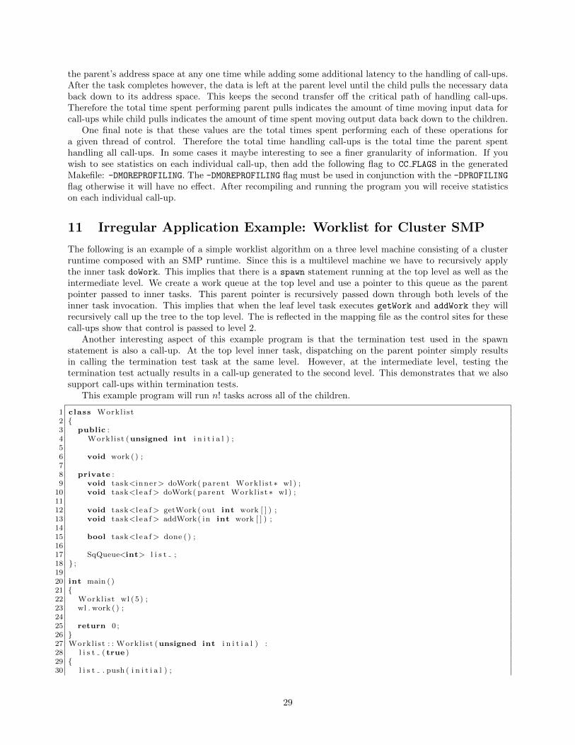
the parent’s address space at any one time while adding some additional latency to the handling of call-ups.After the task completes however, the data is left at the parent level until the child pulls the necessary databack down to its address space. This keeps the second transfer off the critical path of handling call-ups.Therefore the total time spent performing parent pulls indicates the amount of time moving input data forcall-ups while child pulls indicates the amount of time spent moving output data back down to the children.
One final note is that these values are the total times spent performing each of these operations fora given thread of control. Therefore the total time handling call-ups is the total time the parent spenthandling all call-ups. In some cases it maybe interesting to see a finer granularity of information. If youwish to see statistics on each individual call-up, then add the following flag to CC FLAGS in the generatedMakefile: -DMOREPROFILING. The -DMOREPROFILING flag must be used in conjunction with the -DPROFILING
flag otherwise it will have no effect. After recompiling and running the program you will receive statisticson each individual call-up.
11 Irregular Application Example: Worklist for Cluster SMP
The following is an example of a simple worklist algorithm on a three level machine consisting of a clusterruntime composed with an SMP runtime. Since this is a multilevel machine we have to recursively applythe inner task doWork. This implies that there is a spawn statement running at the top level as well as theintermediate level. We create a work queue at the top level and use a pointer to this queue as the parentpointer passed to inner tasks. This parent pointer is recursively passed down through both levels of theinner task invocation. This implies that when the leaf level task executes getWork and addWork they willrecursively call up the tree to the top level. The is reflected in the mapping file as the control sites for thesecall-ups show that control is passed to level 2.
Another interesting aspect of this example program is that the termination test used in the spawnstatement is also a call-up. At the top level inner task, dispatching on the parent pointer simply resultsin calling the termination test task at the same level. However, at the intermediate level, testing thetermination test actually results in a call-up generated to the second level. This demonstrates that we alsosupport call-ups within termination tests.
This example program will run n! tasks across all of the children.
1 class Workl i st2 {3 public :4 Workl i st (unsigned int i n i t i a l ) ;56 void work ( ) ;78 private :9 void task<inner> doWork( parent Workl i st ∗ wl ) ;
10 void task<l e a f > doWork( parent Workl i st ∗ wl ) ;1112 void task<l e a f > getWork ( out int work [ ] ) ;13 void task<l e a f > addWork( in int work [ ] ) ;1415 bool task<l e a f > done ( ) ;1617 SqQueue<int> l i s t ;18 } ;1920 int main ( )21 {22 Workl i st wl (5 ) ;23 wl . work ( ) ;2425 return 0 ;26 }27 Workl i st : : Workl i s t (unsigned int i n i t i a l ) :28 l i s t ( true )29 {30 l i s t . push ( i n i t i a l ) ;
29
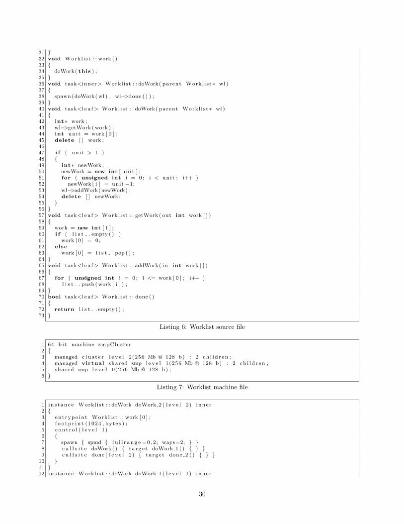
31 }32 void Workl i st : : work ( )33 {34 doWork( this ) ;35 }36 void task<inner> Workl i st : : doWork( parent Workl i st ∗ wl )37 {38 spawn (doWork( wl ) , wl−>done ( ) ) ;39 }40 void task<l e a f > Workl i st : : doWork( parent Workl i st ∗ wl )41 {42 int∗ work ;43 wl−>getWork ( work ) ;44 int uni t = work [ 0 ] ;45 delete [ ] work ;4647 i f ( un i t > 1 )48 {49 int∗ newWork ;50 newWork = new int [ un i t ] ;51 for ( unsigned int i = 0 ; i < uni t ; i++ )52 newWork [ i ] = unit −1;53 wl−>addWork(newWork) ;54 delete [ ] newWork ;55 }56 }57 void task<l e a f > Workl i st : : getWork ( out int work [ ] )58 {59 work = new int [ 1 ] ;60 i f ( l i s t . empty ( ) )61 work [ 0 ] = 0 ;62 else63 work [ 0 ] = l i s t . pop ( ) ;64 }65 void task<l e a f > Workl i st : : addWork( in int work [ ] )66 {67 for ( unsigned int i = 0 ; i <= work [ 0 ] ; i++ )68 l i s t . push ( work [ i ] ) ;69 }70 bool task<l e a f > Workl i st : : done ( )71 {72 return l i s t . empty ( ) ;73 }
Listing 6: Worklist source file
1 64 b i t machine smpCluster2 {3 managed c l u s t e r l e v e l 2(256 Mb @ 128 b) : 2 c h i l d r e n ;4 managed virtual shared smp l e v e l 1(256 Mb @ 128 b) : 2 c h i l d r e n ;5 shared smp l e v e l 0(256 Mb @ 128 b) ;6 }
Listing 7: Worklist machine file
1 in s t ance Workl i st : : doWork doWork 2 ( l e v e l 2) inne r2 {3 ent rypo int Workl i st : : work [ 0 ] ;4 f o o t p r i n t (1024 , bytes ) ;5 c o n t r o l ( l e v e l 1)6 {7 spawn { spmd { f u l l r a n g e =0 ,2; ways=2; } }8 c a l l s i t e doWork ( ) { t a r g e t doWork 1 ( ) { } }9 c a l l s i t e done ( l e v e l 2) { t a r g e t done 2 ( ) { } }
10 }11 }12 in s t ance Workl i st : : doWork doWork 1 ( l e v e l 1) inne r
30

13 {14 f o o t p r i n t (1024 , bytes ) ;1516 c o n t r o l ( l e v e l 0)17 {18 spawn{ spmd { f u l l r a n g e =0 ,2; ways=2; } }19 c a l l s i t e doWork ( ) { t a r g e t doWork 0 ( ) {} }20 c a l l s i t e done ( l e v e l 2) { t a r g e t done 2 ( ) {} }21 }22 }23 in s t ance Workl i st : : doWork doWork 0 ( l e v e l 0) l e a f24 {25 f o o t p r i n t (1024 , bytes ) ;26 c o n t r o l ( l e v e l 2)27 {28 c a l l s i t e getWork ( ) { t a r g e t getWork 2 ( ) {} }29 c a l l s i t e addWork ( ) { t a r g e t addWork 2 ( ) {} }30 }31 }32 in s t ance Workl i st : : getWork getWork 2 ( l e v e l 2) l e a f { f o o t p r i n t (1024 , bytes ) ; }33 in s t ance Workl i st : : addWork addWork 2 ( l e v e l 2) l e a f { f o o t p r i n t (1024 , bytes ) ; }34 in s t ance Workl i st : : done done 2 ( l e v e l 2) l e a f { f o o t p r i n t (1024 , bytes ) ; }
Listing 8: Worklist mapping file
12 The Sequoia GPU Backend
In this section we describe a GPU backend for Sequoia that targets NVIDIA’s CUDA programming language[4]. Targeting a general purpose GPU language such as CUDA was a challenge and forced us to impose somerestrictions on what can be written in a task that will eventually be mapped onto a GPU. We developedour CUDA backend based on CUDA 2.3, and have yet to extend Sequoia’s backend for the new Fermiarchitecture [7]. Fermi should allow us to relax some of the restrictions that we have currently imposed. Wehave tested our CUDA backend on both CUDA 2.3 and CUDA 3.0. Any earlier versions of CUDA will notwork as we make use of some of the more recently added features of the CUDA language.
12.1 Supported Syntax for GPU’s
The current GPU backend for Sequoia requires the programmer to strictly adhere to the traditional Sequoialanguage. This means that all of the additional syntax structures added in section 5 are not supported forGPU’s. Inner tasks are only allowed to consist of tunable declarations and mapping statements. Leaf tasksare slightly less restrictive as we support all of the C syntax supported by CUDA in the leaf tasks. Theprogrammer can therefore still use for, while, and if/else statements in leaf tasks. However, there is nonotion of memory management in leaf tasks as there is no mechanism for allocating data dynamically withina GPU thread. In addition to this, there cannot be any function calls performed at the leaf level 6. We havenot implemented the mapreduce mapping statement for CUDA yet. Finally, we do not support any of theextensions for dynamic parallelism outlined in Section 10 for CUDA.
12.2 Representing GPU’s in Sequoia
In order to map a Sequoia program onto a GPU, it is first necessary to understand the GPU memoryhierarchy. For the purposes of this section we only consider a single GPU machine. We discuss multi-GPUmachines in Section 12.4. In Sequoia we model the GPU memory hierarchy as a four level machine. The toplevel of the machine is the CPU’s main memory. There is only a single child from the CPU main memoryand this level represents the GPU’s device main memory that is off chip. From the device main memory we
6The NVIDIA compiler nvcc supports device level function calls which it then inlines, however, in order to support thisin Sequoia, we would have to clone a function so that we could have both a CPU and GPU version of the function. We currentlydon’t support this, but it would not be a major challenge to add
31

then model the next level as a nearly unbounded7 number of children each with 16KB of memory. This levelis designed to correspond directly to the number of threadblocks the device can launch. We therefore are notmodeling the hardware directly, but rather the number of hardware contexts the GPU is able to support atany one time. The 16KB of memory at this level represents the amount of on-chip shared memory availableto each individual threadblock. Finally, for the last level there are 512 children for each node in the previouslevel. This corresponds to CUDA supporting up to 512 threads per threadblock. It should be noted thatwe make the size of each thread’s local memory at the bottom most level 16KB as well. We will explain thereasons for this in Section 12.3. Below is an example CUDA machine file.
32 bit machine cuda
{
managed shared cudaCpu level 3(4096 Mb @ 16b) : 1 child;
cudaDevice level 2(1024 Mb @ 16b) : 1073741824 children;
cudaThreadBlock level 1(16 Kb @ 4b) : 512 children;
cudaThread level 0(16 Kb @ 4b);
}
There are a couple of things to notice about this machine file. First, we change the byte alignment from 16bytes in the top levels to 4 bytes in the actual device. The reason for this is that CUDA devices assume fourbyte alignments. It is also possible to reduce the CPU side alignments down to 4 bytes if desired. Anotherimportant thing to notice is that this machine only supports a single GPU. If multiple GPU’s are to be usedthen only the term cudaCpu had to be replaced by cudaCMP and the number of children in level 3 modifiedto match the number of GPU’s. The cudaCMP runtime will be explained in more detail in Section 12.4.
12.3 Mapping Tasks onto GPU’s
Now that we have described how to model a GPU in Sequoia, we can discuss how to map tasks onto theGPU. Whenever a task is mapped onto a GPU, it must make use of all four levels. The reason for this isthat in the two intermediate levels, device main memory and threadblock shared memory, there does notexist an actual processor that could explicitly be used for executing leaf tasks. In addition to this the CUDAarchitecture mandates that at least 32 threads must be launched for every threadblock. Therefore we alsorequire that at least 32 tasks must be launched for each task call made in a task running at the threadblocklevel.
The goal in mapping a task onto a GPU is to pack the threadblock level to make use of the restricted16KB of data available as on-chip shared memory. Sequoia doesn’t model the GPU’s registers or localmemory as we assume that the Sequoia generated code will use up most of the registers and local memoryis off-chip 8. We also make use of the fact that Sequoia semantics require that there is no output aliasingbetween tasks, therefore threads at the base level copy data into the shared memory, but then work directlyout of the shared memory. Since each leaf task’s working set is always a subset of its parent’s inner taskworking set, we can guarantee that by packing the level 1 memory, then we are making the best use of theon-chip shared memory. This is the reason that we make the level 0 memory size equal to the level 1 memorysize as we are encouraging the programmer to pack the level 1 memory efficiently. It is important to noticethat there exists the slight possibility to violate Sequoia’s copy-in, copy-out semantics here if the same arrayas passed as both an in argument and an out argument to the leaf level tasks. Since the threads are nolonger copying into their own address space, there will be data races on the reads and writes to the array inthe shared memory. We are still working on implementing this analysis in the compiler, but at the momentit is up to the programmer to be able to perform this operation explicitly.
An additional trick that we encourage the programmer to make use of is that of using the mappingfrom level 3 to level 2 to move as much data in bulk as possible. Ideally, the iteration space of a mappingstatement that goes from level 3 to level 2 should only contain a single iteration. The effect that this willhave is to move all the data down to the device level in a single bulk transfer. This will minimize the pain of
7NVIDIA currently caps the maximum number of threadblocks that can be launched in a kernel call at 232. Unfortunatelywe can only support 230 threadblocks as Sequoia currently uses integers and not long integers to represent machine size.
8We also don’t model the constant or texture caches, but we see a chance for the compiler to make use of these. For example,one potential use would be to place in arguments in the constant cache
32
going across the PCI-Express bus from the CPU main memory to the GPU main memory. It is importantto minimize the number of these transfers as they are very expensive.
In some cases when mapping a Sequoia program onto a GPU, the generated code will use more registersor local memory than is available on a given device. The reason for this is that Sequoia only modelspacking the device main memory and the shared memory of the device. As a result of this the compilerdoesn’t attempt to pack the registers or the local data for the device. It is therefore possible that the compilergenerates code that the NVIDIA compiler nvcc claims cannot be scheduled on the device. The best solutionto this problem is to use fewer threads per threadblock, thereby freeing up more registers. If you want tosee how many registers are currently required for a program, append the option --ptxas-options=-v flagto the NVCC FLAGS in the generate Makefile and recompile. This will then generate a report that will showhow many registers are required for each thread and allow for a more informed decision on the maximumnumber of threads that can be launched on the current device for a given program.
The last thing to consider when mapping programs onto GPU’s is performance. Both the copy eliminationand loop-fusion optimizations described in section 9.4 are still applicable to CUDA. The only optimizationnot fully supported is software pipelining. Software pipelining is supported between levels 2 and 3, but is notsupported anywhere else as there is no way to issue asynchronous data transfers on the GPU. Finally, themappar statement is the optimal choice for scheduling tasks on the GPU as it allows all of the threadblockand the threads to run in parallel. The mapseq statement is supported for CUDA, but has very poorperformance. At the threadblock level a mapseq statement will result in as many kernel calls as there arepoints in the iteration space and only a single threadblock being launched at a time. Similarly, at the threadlevel, a mapseq statement will result in all the threads running their computation as many times as their arepoints in the iteration space, with only one thread being allowed to write its results back after each iteration.In general mapseq can be used for developing an algorithm, but should be avoided if good performance isdesired.
12.4 Targeting a Cluster of GPU’s
One of our primary targets for this version of the Sequoia compiler is a cluster of GPU’s. In our view, acluster of GPU’s could consist of two potential architectures: a single desktop machine that contains multipleGPU’s, or an MPI cluster where each node contains one or more GPU’s as accelerators for the chip(s) on anode. We support both of these architectures.
To support multiple GPU’s we have added the cudaCMP runtime. This will serve as the top level runtimein any process that targets multiple GPU’s. The cudaCMP runtime is based on the SMP runtime describedin Section 6.2. This runtime contains a top level thread that acts as the distributor of work, and then asingle thread for each GPU that is to be targeted. The reason that a separate thread is required is thatNVIDIA stipulates that there be a single thread that controls each device [4]. Below this level, we have thesame three levels as the single GPU runtime described in section 12.3: cudaDevice, cudaThreadBlock, andcudaThread. The only difference between the cudaCMP runtime and cudaCpu runtime is that the cudaCMP
runtime allows the programmer to spread tasks over more than one GPU.The only restriction on the cudaCMP runtime is that it be the top level runtime in a given process. This
is because the runtime assumes that each of the child threads that it creates have a globally unique threadidentification number that will correspond to the CUDA device that they will be targeting. If anotherruntime such as SMP where to be placed on top of the cudaCMP runtime then a situation could occur wherethere are multiple instances of the cudaCMP runtime and the thread ID’s assigned to its children will no longerbe globally unique. This would result in multiple threads trying to control the same GPU and would almostcertainly lead to some form of memory corruption. The one exception to this restriction is the cluster
runtime. The cluster runtime is able to be placed on top of the cudaCMP runtime as the cluster runtimewill generate a separate MPI process for each node, and therefore the cudaCMP runtime is ensured that it isthe only runtime managing the GPU’s on a given node. By composing the cluster and cudaCMP runtimesit is possible to run on an arbitrarily large cluster of GPU’s.
33
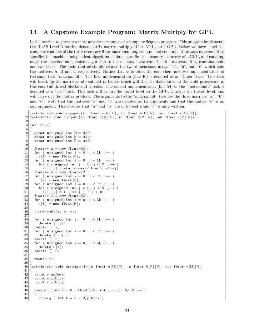
13 A Capstone Example Program: Matrix Multiply for GPU
In this section we present a more advanced example of a complete Sequoia program. This program implementsthe BLAS Level 3 routine dense matrix-matrix multiply (C = A*B), on a GPU. Below we have listed thecomplete contents of the three necessary files: matrixmult.sq, cuda.m, and cuda.mp. As always matrixmult.sqspecifies the machine independent algorithm, cuda.m specifies the memory hierarchy of a GPU, and cuda.mpmaps the machine independent algorithm to the memory hierarchy. The file matrixmult.sq contains mainand two tasks. The main routine simply creates the two dimensional arrays “a”, “b”, and “c” which holdthe matrices A, B and C respectively. Notice that as is often the case there are two implementations ofthe same task ”matrixmult”. The first implementation (line 40) is denoted as an ”inner” task. This taskwill break up the matrices into submatrix blocks which will then be distributed to the child processors, inthis case the thread blocks and threads. The second implementation (line 54) of the “matrixmult” task isdenoted as a “leaf” task. This task will run at the lowest level on the GPU, which is the thread level, andwill carry out the matrix product. The arguments to the “matrixmult” task are the three matrices “a”, “b”,and “c”. Note that the matrices “a” and “b” are denoted as in arguments and that the matrix “c” is anout argument. This ensures that “a” and “b” are only read while “c” is only written.
1 task<inner> void compute ( in f loat a [M] [ P ] , in f loat b [P ] [ N] , out f loat c [M] [ N] ) ;2 task<l e a f > void compute ( in f loat a [M] [ P ] , in f loat b [P ] [ N] , out f loat c [M] [ N] ) ;34 int main ( )5 {6 const unsigned int M = 256 ;7 const unsigned int N = 256 ;8 const unsigned int P = 256 ;9
10 f loat ∗∗ a = new float ∗ [M] ;11 for ( unsigned int i = 0 ; i < M; i++ )12 a [ i ] = new float [P ] ;13 for ( unsigned int i = 0 ; i < M; i++ )14 for ( unsigned int j = 0 ; j < P; j++ )15 a [ i ] [ j ] = static cast<f loat>( i ∗10+ j ) ;16 f loat ∗∗ b = new float ∗ [P ] ;17 for ( unsigned int i = 0 ; i < P; i++ )18 b [ i ] = new float [N ] ;19 for ( unsigned int i = 0 ; i < P; i++ )20 for ( unsigned int j = 0 ; j < N; j++ )21 b [ i ] [ j ] = ( i == j ) ? 1 : 0 ;22 f loat ∗∗ c = new float ∗ [M] ;23 for ( unsigned int i = 0 ; i < M; i++ )24 c [ i ] = new float [N ] ;2526 matrixmult ( a , b , c ) ;2728 for ( unsigned int i = 0 ; i < M; i++ )29 delete [ ] a [ i ] ;30 delete [ ] a ;31 for ( unsigned int i = 0 ; i < P; i++ )32 delete [ ] b [ i ] ;33 delete [ ] b ;34 for ( unsigned int i = 0 ; i < M; i++ )35 delete c [ i ] ;36 delete [ ] c ;3738 return 0 ;39 }40 task<inner> void matrixmult ( in f loat a [M] [ P ] , in f loat b [P ] [ N] , out f loat c [M] [ N] )41 {42 tunable mBlock ;43 tunable pBlock ;44 tunable nBlock ;4546 mappar ( int i = 0 : M/mBlock , int j = 0 : N/nBlock )47 {48 mapseq ( int k = 0 : P/pBlock )
34

49 {50 matrixmult ( a [ i ∗mBlock ; mBlock ] [ k∗pBlock ; pBlock ] , b [ k∗pBlock ; pBlock ] [ j ∗nBlock ; nBlock ] , c
[ i ∗mBlock ; mBlock ] [ j ∗nBlock ; nBlock ] ) ;51 }52 }53 }54 task<l e a f > void matrixmult ( in f loat a [M] [ P ] , in f loat b [P ] [ N] , out f loat c [M] [ N] )55 {56 for ( unsigned int i = 0 ; i < M; i++ )57 for ( unsigned int j = 0 ; j < N; j++ )58 {59 c [ i ] [ j ] = 0 . 0 ;60 for ( unsigned int k = 0 ; k < P; k++ )61 c [ i ] [ j ] += a [ i ] [ k ] ∗ b [ k ] [ j ] ;62 }63 }
Listing 9: Matrix Multiply source file
The machine file, cuda.m, contains a description of an NVIDIA GPU on which we will run this application.A GPU has four memory levels in Sequoia: cudaCPU, cudaDevice, cudaThreadBlock, and cudaThread. ThecudaCPU level describes the main memory and host CPU which will launch and create the data for thecomputation. The cudaDevice level describes the device main memory on the GPU. The cudaThreadBlock
level describes the first level of parallelism on a GPU, namely the thread blocks. The bottom level inthe hierarchy then is the cudaThread level which as it sounds describes the individual threads within eachthreadblock. The cuda runtime was written with separate memory levels for the threadblock and threadparallelism so that the programmer has more control over how work is divided up on the GPU. This wayit is possible to specify the number of threadblocks created as well as threads per thread block. The child
keywords in this machine file tell Sequoia that there are a total of 100 million thread blocks possible eachwith 512 threads. The fact that we can allow up to 100 million thread blocks is a feature of cuda whichallows more thread blocks to be created than there are hardware contexts. The thread blocks are thenscheduled appropriately by cuda. The memory restrictions of the GPU platform are also described, level 2sets the device main memory at 1024 Mb aligned on 16 byte boundaries and level 0 sets the memory size ofthe registers to be 16 kilobytes aligned on 4 byte boundaries.
1 32 b i t machine cuda2 {3 managed cudaCpu l e v e l 3(4096 Mb @ 16 b) : 1 c h i l d ;4 cudaDevice l e v e l 2(1024 Mb @ 16 b) : 4294967296 c h i l d r e n ; // 2ˆ325 cudaThreadBlock l e v e l 1(16 Kb @ 4 b) : 512 c h i l d r e n ;6 cudaThread l e v e l 0(16 Kb @ 4 b) ;7 }
Listing 10: Matrix Multiply machine file
The mapping file, cuda.mp, describes to Sequoia how the abstract algorithm contained in matrixmult.sqis to be applied to the GPU described in cuda.m. For this example four instances of the task “matrixmult”(“i1”, “i2”, “i3” , and “i4” as seen below) are created. Each instance of the “inner” implementation ofthe “matrixmult” task defines concrete values for the tunables “mBlock”, “nBlock”, and “pBlock”. Thesetunables are used by the algorithm in matrixmult.sq as the dimensions of the submatrices to be to be passedto the recursive “matrixmult” call. The topmost instance, “i1”, instantiated on level 3 contains a data
section which defines the initial size of the matrices. So at level 3, on the CPU, the matrices are determinedto be 256x256. Also “i1” sets “mBlock”, “nBlock”, and “pBlock” to be 256. Since “i1” is instantiate forlevel 3 this implies that the matrices sent to level 2 will be size 256x256 also. This implies that the entirematrices will be passed from the CPU to the GPU device. Next instance “i2” sets the tunables to 1, 1, and 32respectively. This has the effect of making the matrices sent to level 1 non-square so that “a” is 1x32, “b” is32x1, and “c” is 1x1. Lastly “i3” on level 1 assigns the tunables the values 1, 1, 1 so that the matrices passedto level 0 are all dimension 1x1. In this way the matrices are broken up from level to level until they reachthe bottom of the hierarchy and the cuda threads operate on single matrix elements. The instances of theinner implementation of “matrixmult” also contain a control section. The control sections describe howthe two dimensional mappar loop and the one dimensional mapseq loop are to distribute the submatrix blocks
35

among the child processes at each level. In instance “i1” on level 3 since there is only one child of the CPU,namely the GPU device, the spmd width of both of the mappar dimensions is 1. This corresponds correctlyto the iteration bounds for “i”, “j”, and “k” which are calculated as N
nBlock = 256256 = 1, M
mBlock = 256256 = 1,
and PpBlock = 256
256 = 1 respectively so that each dimension of the loops has only one iteration. This impliesthat there is no parallelism or looping from level 3 to level 2 as expected and so the 256x256 matrices aresimply copied from the CPU to the GPU in their entirety. On level 2 in instance “i2”, however, we now havethe ways of the two mappar dimensions specified as 256. This gives the iteration bounds on “i” and “j” as
NnBlock = 256
1 = 256 and MmBlock = 256
1 = 256. So the two dimensional mappar on level 2 will iterate throughall 256 of the rows in “a” and for each of those rows it will iterate through all 256 columns of “b”. Now since“pBlock” is not the full 256 but is set to 32, we will not be transferring the whole rows of “a” or the wholecolumns of “b” all at once. Instead each row and each column will be broken up into 8, 32 element pieces.These sub-rows and sub-columns are then what are sent to level 1. Since we know from the machine filethat level 1 represents the thread block level this data partitioning describes a total of 524288 thread blocksto be launched on the GPU. Interesting to note is the fact that the mapseq loop, the innermost loop, has aspecified spmd ways which breaks up dependent parts of the data. Namely the resulting products computedfrom the sub-rows and sum-columns created from “a” and “b” are not independent of each other when theybelong to the same row/column. Dividing dependent computations in this way is a safe thing to do whenthe looping construct is a mapseq. In this case the spmd distributed computations will be computed byseparate thread blocks but the mapseq will ensure that the computations happen in order and one at a time.This is also what happens on level 0. The matrices on level 0 have sizes “a”: 1x32, “b”:32x1, and “c”:1x1and so only the inner dimension is further divided up. This again is safe to do because the inner dimensionis divided up using a mapseq loop which preserves order and serializes the individual computations. Sothe mapping file describes data being broken up progressively as it moves down through the levels so thateach cuda thread ends up multiplying one element of “a” times one element of “b” and adding them to theaccumulating corresponding element of “c”.
1 in s t ance matrixmult i 1 ( l e v e l 3) inner2 {3 ent rypo int main [ 0 ] ;4 tunable mBlock = 256 ;5 tunable nBlock = 256 ;6 tunable pBlock = 256 ;7 data ( )8 {9 array a ( ) { e lements = 256 ,256 ; }
10 array b ( ) { e lements = 256 ,256 ; }11 array c ( ) { e lements = 256 ,256 ; }12 }13 c o n t r o l ( l e v e l 2)14 {15 loop i ( ) { spmd { f u l l r a n g e = 0 , 1 ; ways = 1 ; i t e r b l k = 1 ; } }16 loop j ( ) { spmd { ways = 1 ; i t e r b l k = 1 ; } }17 loop k ( ) { }18 c a l l s i t e matrixmult ( ) { t a r g e t i 2 ( ) { } }19 }20 }21 in s t ance matrixmult i 2 ( l e v e l 2) inner22 {23 tunable mBlock = 1 ;24 tunable nBlock = 1 ;25 tunable pBlock = 32 ;26 c o n t r o l ( l e v e l 1)27 {28 loop i ( ) { spmd { f u l l r a n g e = 0 ,524288 ; ways = 256 ; i t e r b l k = 1 ; } }29 loop j ( ) { spmd { ways = 256 ; i t e r b l k = 1 ; } }30 loop k ( ) { spmd { ways = 8 ; i t e r b l k = 1 ;} }31 c a l l s i t e matrixmult ( ) { t a r g e t i 3 ( ) { } }32 }33 }34 in s t ance matrixmult i 3 ( l e v e l 1) inner35 {36 tunable mBlock = 1 ;
36

37 tunable nBlock = 1 ;38 tunable pBlock = 1 ;39 c o n t r o l ( l e v e l 0)40 {41 loop i ( ) { spmd { f u l l r a n g e = 0 ,32 ; ways = 1 ; i t e r b l k = 1 ; } }42 loop j ( ) { spmd { ways = 1 ; i t e r b l k = 1 ; } }43 loop k ( ) { spmd { ways = 32 ; i t e r b l k = 1 ; } }44 c a l l s i t e matrixmult ( ) { t a r g e t i 4 ( ) { } }45 }46 }47 in s t ance matrixmult i 4 ( l e v e l 0) l e a f { }
Listing 11: Matrix Multiply mapping file
14 Known Issues
• Error locations for errors in inter-file dependency analysis are incorrect
• Some errors are caught by assertions in the compiler instead of being handled explicitly through errormessages
• Task calls across memory levels are only supported through mapping statements
• mapreduce statements currently only work with one dimensional arrays
• There may be false warnings concerning reading from out parameters or writing to in parameters asour static analysis is not sound
• The CUDA runtimes will sometimes not generate correct code with the optimizations from the −Oflag applied
• The compiler cannot support the full width of threadblocks (232) since it represents machine widthsusing integers instead of long integers
• No support for namespaces
References
[1] S. McPeak and D. Wilkerson, “Elsa: The Elkhound-based C/C++Parser,” http://www.cs.berkeley.edu/˜smcpeak/elkhound, 2005. [Online]. Available:http://www.cs.berkeley.edu/ smcpeak/elkhound
[2] M. Houston, J. Y. Park, M. Ren, T. Knight, K. Fatahalian, A. Aiken, W. Dally, and P. Hanrahan,“A portable runtime interface for multi-level memory hierarchies,” in Proceedings of the Symposium onPrinciples and Practice of Parallel Programming, 2008, pp. 143–152.
[3] E. Gabriel, G. E. Fagg, G. Bosilca, T. Angskun, J. J. Dongarra, J. M. Squyres, V. Sahay, P. Kambadur,B. Barrett, A. Lumsdaine, R. H. Castain, D. J. Daniel, R. L. Graham, and T. S. Woodall, “Open MPI:Goals, concept, and design of a next generation MPI implementation,” in Proceedings, 11th EuropeanPVM/MPI Users’ Group Meeting, Budapest, Hungary, September 2004, pp. 97–104.
[4] NVIDIA, “Nvidia cuda programming guide: Version 3.0,” 2010. [Online]. Available:http://developer.nvidia.com/object/cuda 3 0 downloads.html#Linux
[5] T. Knight, J. Y. Park, M. Ren, M. Houston, M. Erez, K. Fatahalian, A. Aiken, W. Dally, and P. Hanrahan,“Compilation for explicitly managed memory hierarchies,” in Proceedings of the Symposium on Principlesand Practice of Parallel Programming, 2007, pp. 226–236.
37

[6] M. Ren, J. Y. Park, M. Houston, A. Aiken, and W. Dally, “A tuning framework for software-managedmemory hierarchies,” in Proceedings of the International Conference on Parallel Architectures and Com-pilation Techniques, 2008, pp. 280–291.
[7] NVIDIA, “Nvidia’s next generation cuda compute architecture: Fermi,” 2009. [Online]. Available:http://www.nvidia.com/object/fermi architecture.html
38


![User Guide...User. {{]}]} {}]}](https://img.pdfslide.net/doc/110x75/60918ca14327954d24291644/-user-guide-user-.jpg)