Session III

Introduction to Basic Data Analysis

Dr. L. JeyaseelanProfessor

Department of BiostatisticsChristian Medical College, Vellore.

About Statistics Class:

Some one said

“ If I had only one day to live,

I would live it in my statistics class -

About Statistics Class (Contd..):

“it would seem so much longer”

What is Statistics?

A science of:

• Collecting numerical information (data)

• Evaluating the numerical information(classify, summarize, organize, analyze)

•Drawing conclusions based on evaluation

Statistical Applications

• Descriptive Statistics

Summarizes or describes the data set at hand. Evaluate the data set for patterns and reduce information to a convenient form.

• Inferential Statistics

Use sample data to make estimates or predictions about a larger set of data.

Types of Data

Qualitative Data Quantitative Data

Nominal Ordinal Discrete Continuous

Interval Ratio

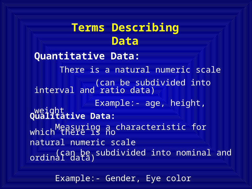
Terms Describing Data

Quantitative Data:There is a natural numeric scale

(can be subdivided into interval and ratio data)

Example:- age, height, weight

Qualitative Data:Measuring a characteristic for which there is no

natural numeric scale (can be subdivided into nominal and ordinal data)

Example:- Gender, Eye color

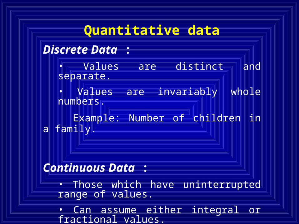
Quantitative data

Discrete Data : • Values are distinct and separate.

• Values are invariably whole numbers.

Example: Number of children in a family.

Continuous Data :• Those which have uninterrupted range of values.

• Can assume either integral or fractional values.

Example : Height, Weight, Age

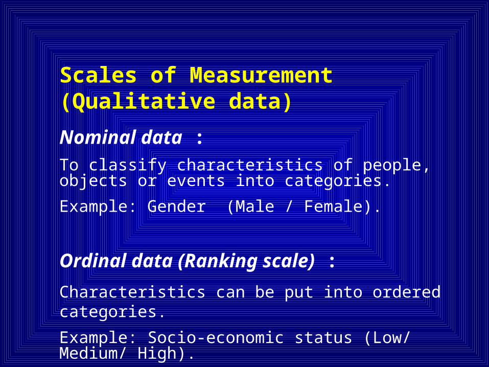
Scales of Measurement (Qualitative data)

Nominal data :

To classify characteristics of people, objects or events into categories.

Example: Gender (Male / Female).

Ordinal data (Ranking scale) :

Characteristics can be put into ordered categories.

Example: Socio-economic status (Low/ Medium/ High).

DESCRIPTIVE STATISTICS

Descriptive Statistics

Measures of central tendency are statistics that summarize a distribution of scores by reporting the most typical or representative value of the distribution.

Measures of dispersion are statistics that indicate the amount of variety or heterogeneity in a distribution of scores.

Descriptive Statistics

• Measures of Central Tendency– Mean– Median– Mode

• Measures of Dispersion– Range– Variance – Standard Deviation

Mean:

• Single value that could describes the characteristics of

the entire data

• Most representative

• Arithmetic mean or average

Mean birth weight, mean DBP

Merits:

Easy to Understand and compute

Based on the value of every item in the series

Limitations:

Affected by extreme values

Not useful for the study of qualities like

intelligence, honesty and character

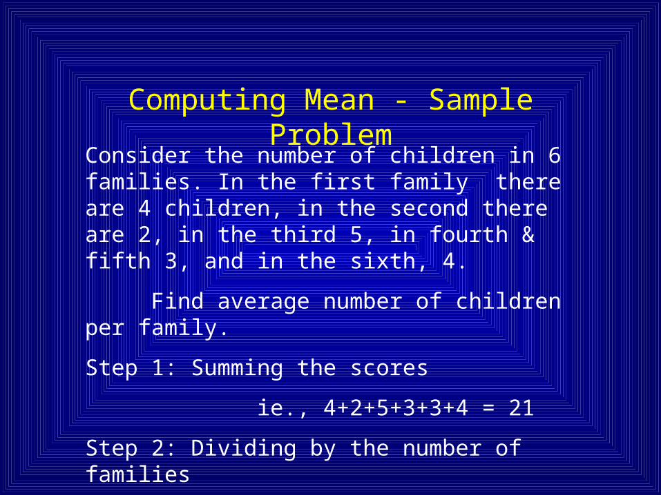
Computing Mean - Sample Problem

Consider the number of children in 6 families. In the first family there are 4 children, in the second there are 2, in the third 5, in fourth & fifth 3, and in the sixth, 4.

Find average number of children per family.

Step 1: Summing the scores

ie., 4+2+5+3+3+4 = 21

Step 2: Dividing by the number of families

ie., 21 ÷ 6 = 3.5

Interpretation:

The average number of children per family is 3.5

Median:

• Arrange the data in ascending or descending order. Middle value is median.

•Not influenced by extreme values

• Unique and easy to calculate

• More appropriate when the measure is Duration (survival), age etc

Computing the Median

• To compute the median, we sort the values from low to high. The median is the middle score.

• If the number of cases in the sample is an odd number, the middle case is the case above and below which the same number of cases occur. ( e.g. 1 2 3 4 5 )

• If the number of cases in the sample is an even number, there will be two middle scores and the median is halfway between these two middle scores. (e.g. 1 2 3 4 5 6 )

Mode:

• Most commonly occurring observation.

• Not Unique.

• Not very frequently used.

• Used in investigation of an epidemic.

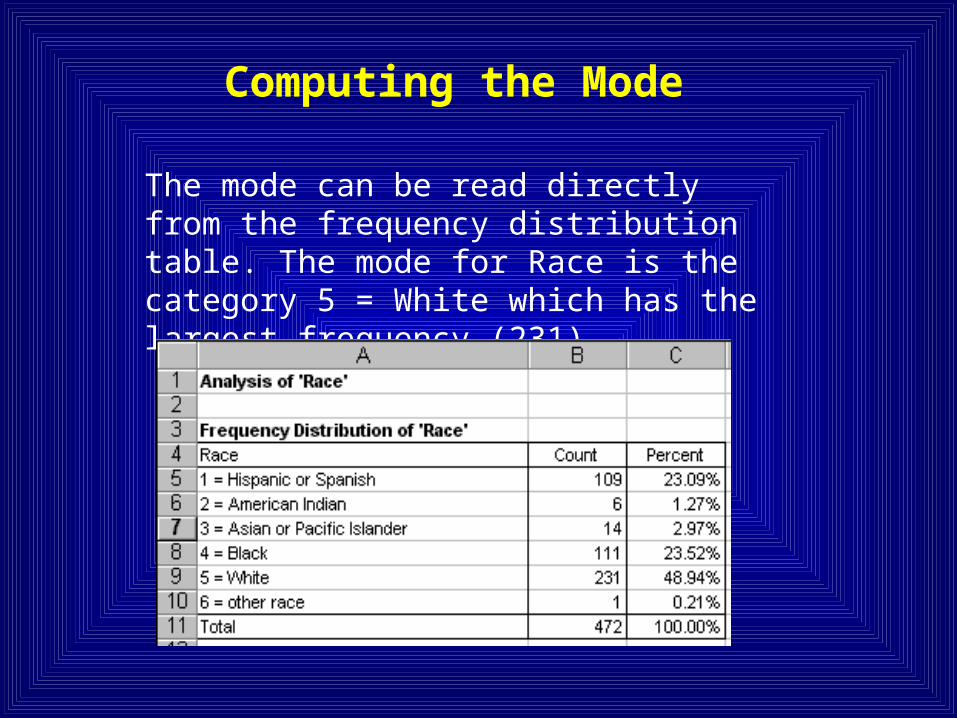
Computing the Mode

The mode can be read directly from the frequency distribution table. The mode for Race is the category 5 = White which has the largest frequency (231).

Is that Enough?

Mean, Median and Mode

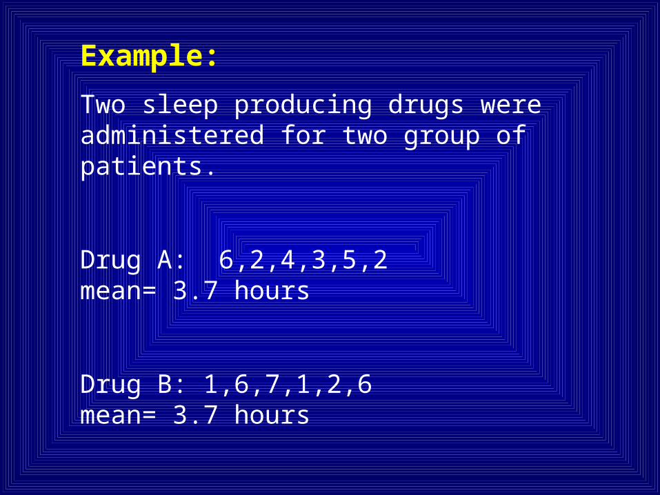
Example:

Two sleep producing drugs were administered for two group of patients.

Drug A: 6,2,4,3,5,2 mean= 3.7 hours

Drug B: 1,6,7,1,2,6 mean= 3.7 hours

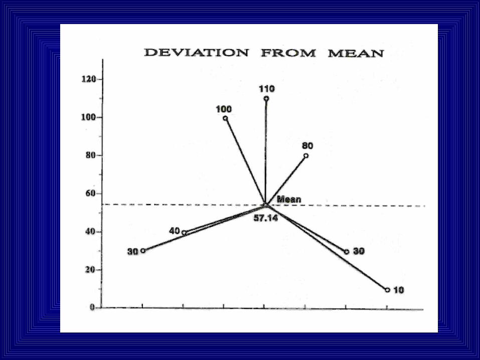
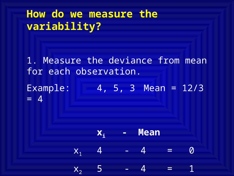
How do we measure the variability?

1. Measure the deviance from mean for each observation.

Example: 4, 5, 3 Mean = 12/3 = 4

xi - Mean

x1 4 - 4 = 0

x2 5 - 4 = 1

x3 3 - 4 = -1

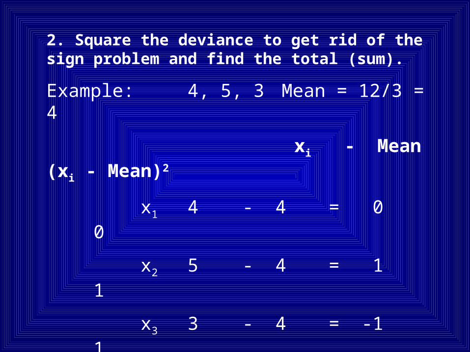
2. Square the deviance to get rid of the sign problem and find the total (sum).

Example: 4, 5, 3 Mean = 12/3 = 4

xi - Mean (xi - Mean)2

x1 4 - 4 = 0 0

x2 5 - 4 = 1 1

x3 3 - 4 = -1 1

Total 0 2

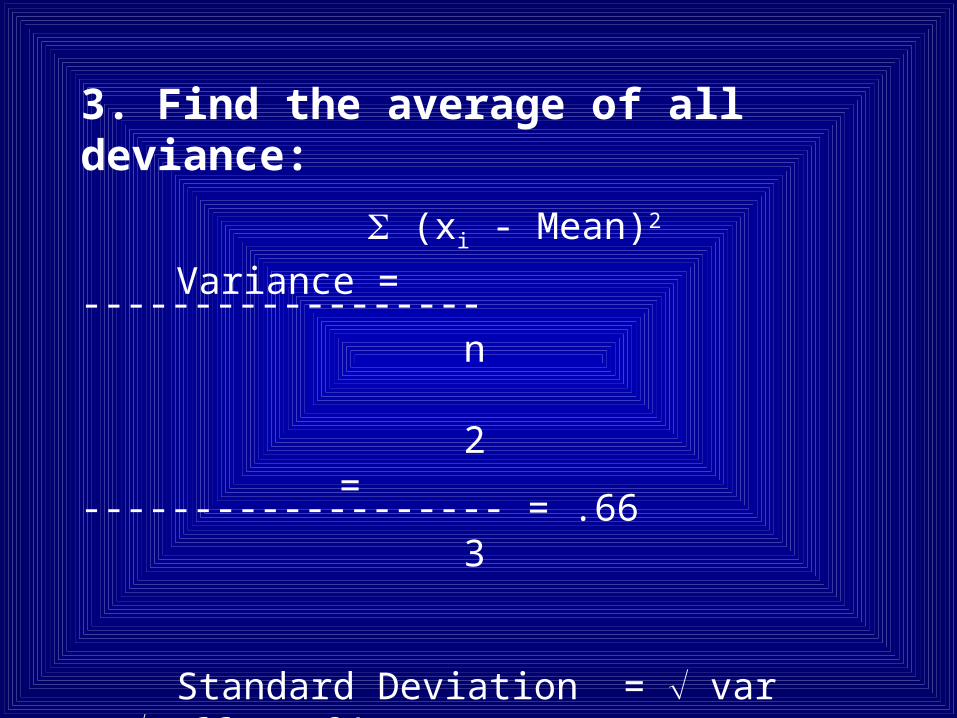
3. Find the average of all deviance:

(xi - Mean)2

Variance = ------------------n

2 = ------------------- = .66

3

Standard Deviation = var = .66 = .81

Variance or Standard Deviation:

On an average, how far each and every observation deviates from the mean.

About the study itself.

Standard Error:• Sample mean is an estimate of the population mean.

• Mean birth weight of 100 babies is 2700g (sd=200).

• Can we say that the population mean is also 2700g?

• Uncertainty associated with our estimate 2700g

• How do we measure the uncertainty?

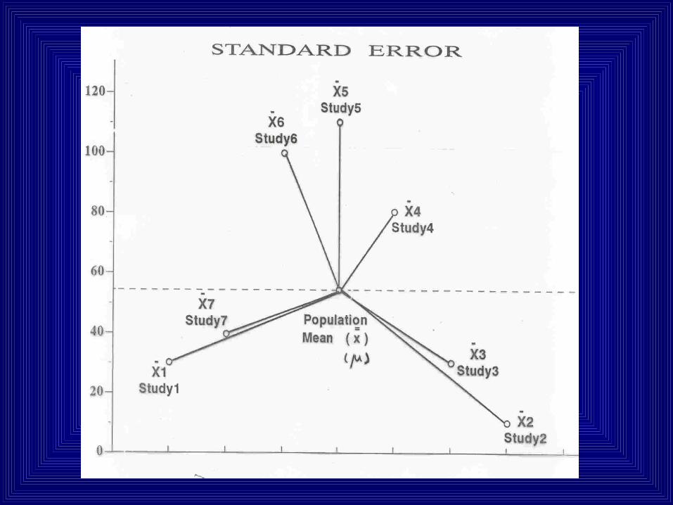
Standard Error (contd..):

Take many samples of same size from the population.

• Assess the variability of such means.

• These means follow Normal distribution.

• Mean of these means is the population mean.

• This variability can be estimated from a single study.

• SE = /n

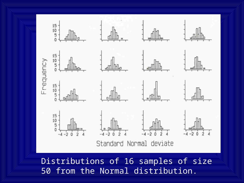
Distributions of 16 samples of size 50 from the Normal distribution.

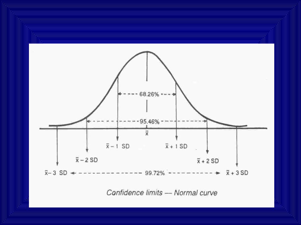
Normal Distribution

• Bell shaped

• Symmetrical about its mean

• Mean, Median and Mode are same

• Total area is one square unit

Point Estimate

The prevalence of HIV in Tamil Nadu was 1.8% in 1998 and .7% in 2003.

As a special honey moon offer we will provide you a double Bed room at the cost of a single room.

Confidence Interval:

• Means of different samples follows normal distribution.

• Mean ± 1.96 SD covers 95% of the area.

• These limits which will cover population mean.

• 5% of the time these limits may not cover the population mean.

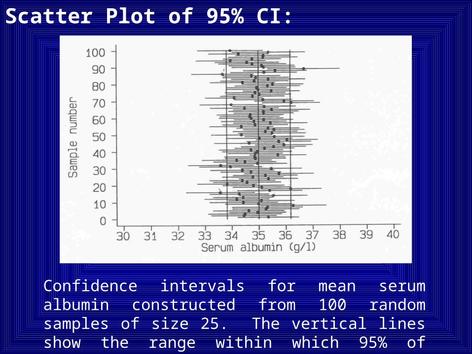
Scatter Plot of 95% CI:

Confidence intervals for mean serum albumin constructed from 100 random samples of size 25. The vertical lines show the range within which 95% of sample means are expected to fall.

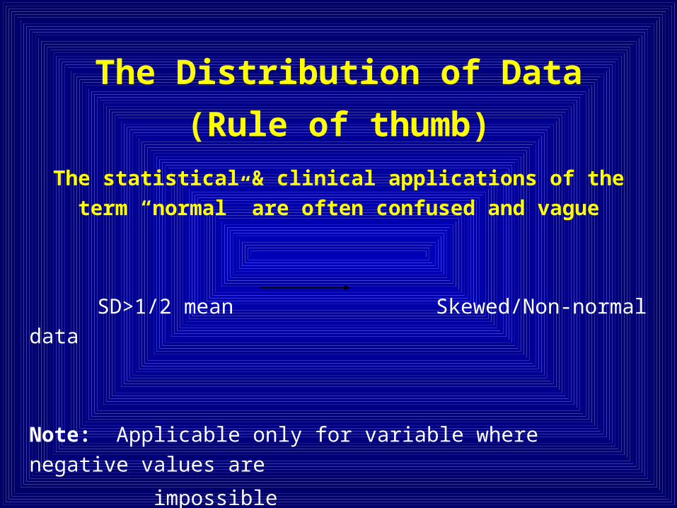
The Distribution of Data

(Rule of thumb)

The statistical & clinical applications of the term “normal” are

often confused and vague

SD>1/2 mean Skewed/Non-normal data

Note: Applicable only for variable where negative values are

impossible

Altman BMJ1991.

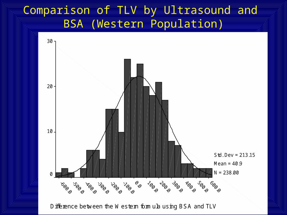
Difference between the W estern formula using BSA and TLV

30

20

10

0

Std. Dev = 213.15

Mean = 40.9

N = 238.00

Comparison of TLV by Ultrasound and BSA (Western Population)

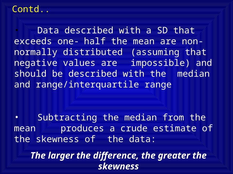
• Data described with a SD that exceeds one-half the mean are non-normally distributed (assuming that negative values are

impossible) and should be described with the median and range/interquartile range

• Subtracting the median from the mean produces a crude estimate of the skewness of

the data:

The larger the difference, the greater the skewness

Contd..

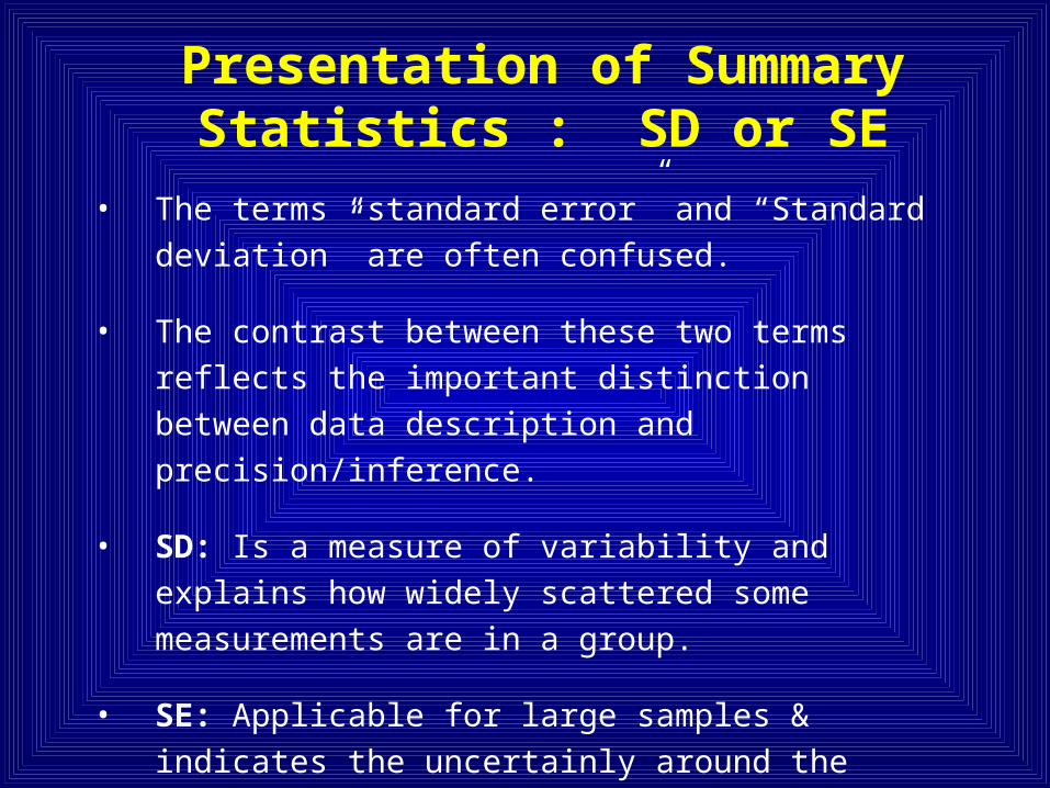
• The terms “standard error” and “Standard deviation” are

often confused.

• The contrast between these two terms reflects the

important distinction between data description and

precision/inference.

• SD: Is a measure of variability and explains how widely

scattered some measurements are in a group.

• SE: Applicable for large samples & indicates the

uncertainly around the estimate of the mean

measurement.

Presentation of Summary Statistics : SD or SE

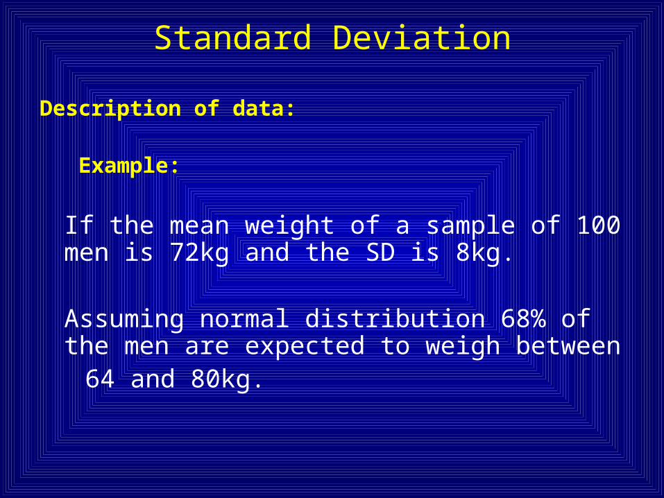
Standard Deviation

Description of data:

Example:

If the mean weight of a sample of 100 men is 72kg and the SD is 8kg.

Assuming normal distribution 68% of the men are expected to weigh between

64 and 80kg.

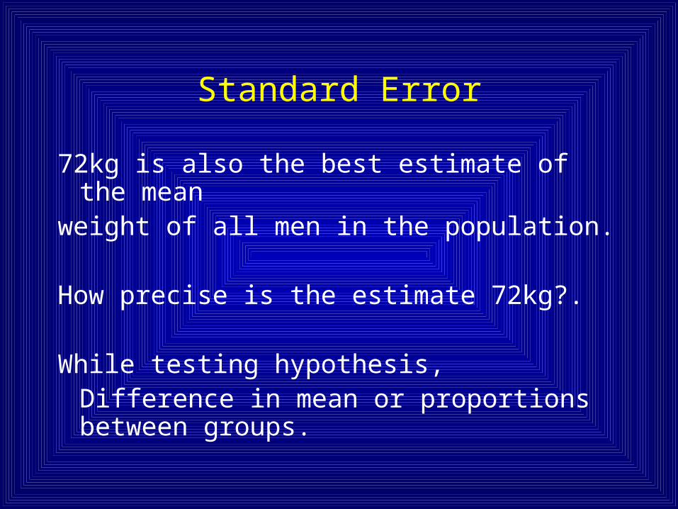
Standard Error

72kg is also the best estimate of the mean weight of all men in the population.

How precise is the estimate 72kg?.

While testing hypothesis,Difference in mean or proportions between groups.

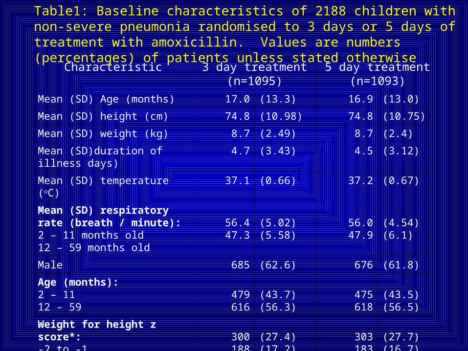
Characteristic 3 day treatment (n=1095)

5 day treatment (n=1093)

Mean (SD) Age (months) 17.0 (13.3) 16.9 (13.0)

Mean (SD) height (cm) 74.8 (10.98) 74.8 (10.75)

Mean (SD) weight (kg) 8.7 (2.49) 8.7 (2.4)

Mean (SD)duration of illness days) 4.7 (3.43) 4.5 (3.12)

Mean (SD) temperature (oC) 37.1 (0.66) 37.2 (0.67)

Mean (SD) respiratory rate (breath / minute):2 – 11 months old12 – 59 months old

56.447.3

(5.02)(5.58)

56.047.9

(4.54)(6.1)

Male 685 (62.6) 676 (61.8)

Age (months):2 – 1112 – 59

479616

(43.7)(56.3)

475618

(43.5)(56.5)

Weight for height z score*:-2 to -1-3 - 2

300188

(27.4)(17.2)

303183

(27.7)(16.7)

Table1: Baseline characteristics of 2188 children with non-severe pneumonia randomised to 3 days or 5 days of treatment with amoxicillin. Values are numbers (percentages) of patients unless stated otherwise

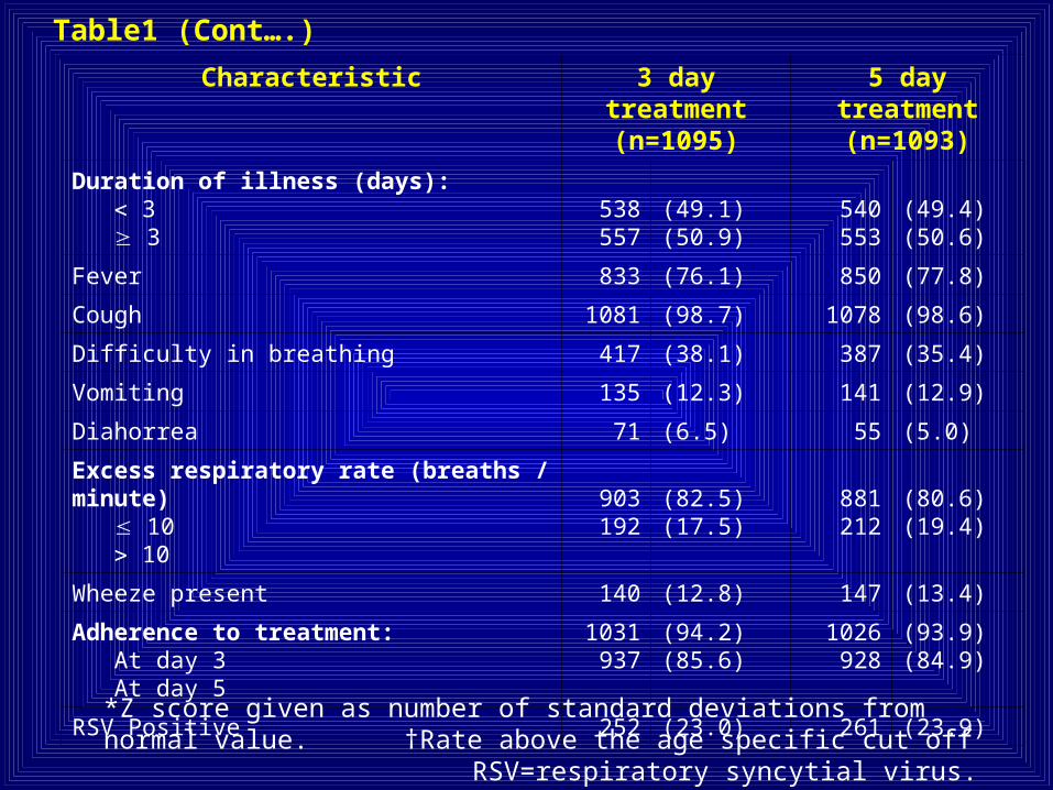
Characteristic 3 day treatment (n=1095)

5 day treatment (n=1093)

Duration of illness (days): 3 3

538557

(49.1)(50.9)

540553

(49.4)(50.6)

Fever 833 (76.1) 850 (77.8)

Cough 1081 (98.7) 1078 (98.6)

Difficulty in breathing 417 (38.1) 387 (35.4)

Vomiting 135 (12.3) 141 (12.9)

Diahorrea 71 (6.5) 55 (5.0)

Excess respiratory rate (breaths / minute) 10 10

903192

(82.5)(17.5)

881212

(80.6)(19.4)

Wheeze present 140 (12.8) 147 (13.4)

Adherence to treatment: At day 3 At day 5

1031937

(94.2)(85.6)

1026928

(93.9)(84.9)

RSV Positive 252 (23.0) 261 (23.9)

Table1 (Cont….)

*Z score given as number of standard deviations from normal value. †Rate above the age specific cut off RSV=respiratory syncytial virus.

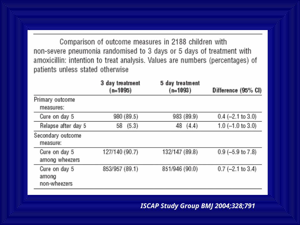
ISCAP Study Group BMJ 2004;328;791

THANKS