Embed Size (px)
Citation preview
1
ISSUE BRIEF
SETTING THE NEXT ROUND OF FUEL ECONOMY STANDARDS:
CONSUMERS BENEFIT AT 60 MILES PER GALLON (OR MORE)
MARK COOPER, DIRECTOR OF RESEARCH
AUGUST 2010
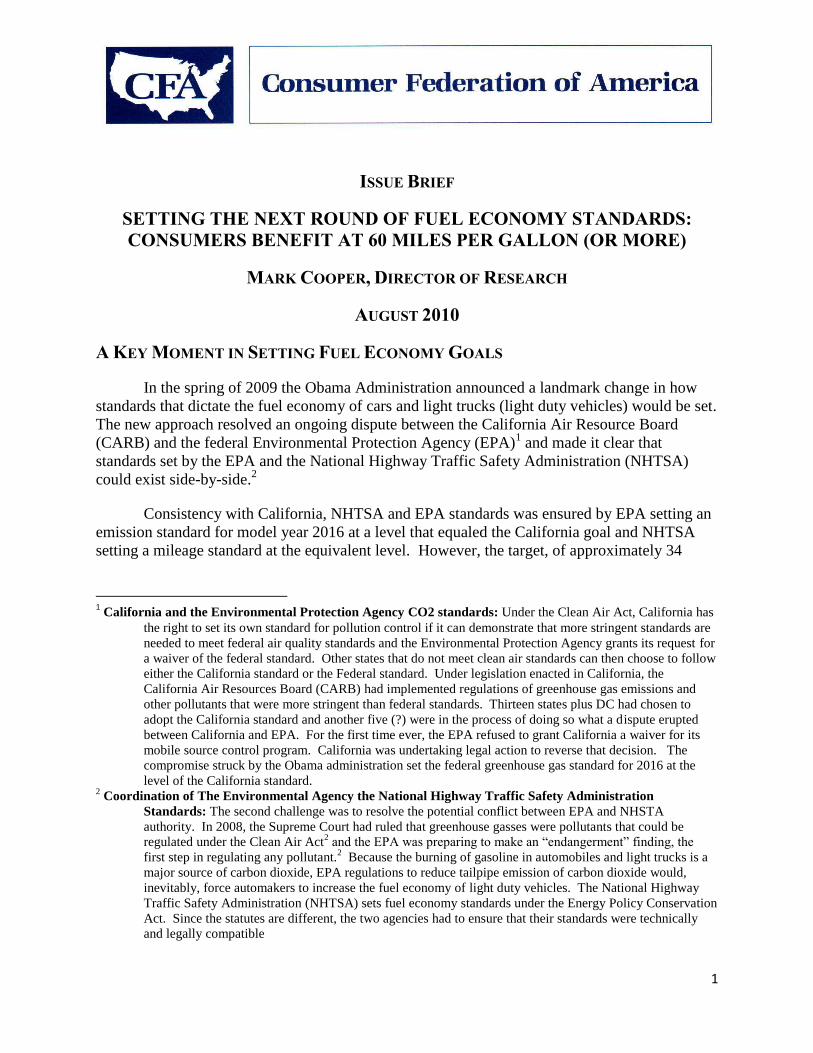
A KEY MOMENT IN SETTING FUEL ECONOMY GOALS
In the spring of 2009 the Obama Administration announced a landmark change in how
standards that dictate the fuel economy of cars and light trucks (light duty vehicles) would be set.
The new approach resolved an ongoing dispute between the California Air Resource Board
(CARB) and the federal Environmental Protection Agency (EPA)1 and made it clear that
standards set by the EPA and the National Highway Traffic Safety Administration (NHTSA)
could exist side-by-side.2
Consistency with California, NHTSA and EPA standards was ensured by EPA setting an
emission standard for model year 2016 at a level that equaled the California goal and NHTSA
setting a mileage standard at the equivalent level. However, the target, of approximately 34
1 California and the Environmental Protection Agency CO2 standards: Under the Clean Air Act, California has
the right to set its own standard for pollution control if it can demonstrate that more stringent standards are
needed to meet federal air quality standards and the Environmental Protection Agency grants its request for
a waiver of the federal standard. Other states that do not meet clean air standards can then choose to follow
either the California standard or the Federal standard. Under legislation enacted in California, the
California Air Resources Board (CARB) had implemented regulations of greenhouse gas emissions and
other pollutants that were more stringent than federal standards. Thirteen states plus DC had chosen to
adopt the California standard and another five (?) were in the process of doing so what a dispute erupted
between California and EPA. For the first time ever, the EPA refused to grant California a waiver for its
mobile source control program. California was undertaking legal action to reverse that decision. The
compromise struck by the Obama administration set the federal greenhouse gas standard for 2016 at the
level of the California standard. 2 Coordination of The Environmental Agency the National Highway Traffic Safety Administration
Standards: The second challenge was to resolve the potential conflict between EPA and NHSTA
authority. In 2008, the Supreme Court had ruled that greenhouse gasses were pollutants that could be
regulated under the Clean Air Act2 and the EPA was preparing to make an “endangerment” finding, the
first step in regulating any pollutant.2 Because the burning of gasoline in automobiles and light trucks is a
major source of carbon dioxide, EPA regulations to reduce tailpipe emission of carbon dioxide would,
inevitably, force automakers to increase the fuel economy of light duty vehicles. The National Highway
Traffic Safety Administration (NHTSA) sets fuel economy standards under the Energy Policy Conservation
Act. Since the statutes are different, the two agencies had to ensure that their standards were technically
and legally compatible
2
miles per gallon for model year 2016 proved to be very modest. The analysis showed that it
would have been economically and environmentally beneficial to set a much higher standard.
This fall, this important reform of energy policy making will be put to the test. Both the
Federal agencies and the California agency will be setting standards for future years. Because
the auto manufacturers need long lead times, fuel economy and greenhouse gas emission
standards for the model year 2017- 2025 period are being considered.
In comments filed in the Federal regulatory proceeding, the Consumer Federation of
America put the administration on notice that, while rationalizing the institutional framework for
setting this important piece of energy policy was a landmark accomplishment, a real victory can
only be claimed when the standards are set at a level that captures the immense benefits that had
been left on the table
It will be critically important for the agencies to move the standard well beyond the
current levels. The regulatory agencies will be doing detail technology assessments and
economic analyses over the next few months. In anticipation of those developments, this paper
reviews the stakes for consumers and the evidence that the standards should be set at much
higher levels.
WHY THE 2016 STANDARDS SHOULD BE HIGHER
Strong Fuel economy and greenhouse gas emission standards are critical to successful
energy and environmental policy not only in the U.S. but globally because the U.S. consumes
one-quarter of the world’s petroleum products and two-fifths of the world’s gasoline. 3
Gasoline
is a major source of the most important global warming greenhouse gas – carbon dioxide.4
Strong standards are also extremely important to consumers because gasoline is a major
expenditure for most American households.5 After housing and food, expenditures on gasoline
are one of the largest items in the household budget, roughly equal to health care expenditures,
50% larger than clothing, twice as large as electricity and four times as large as natural gas.
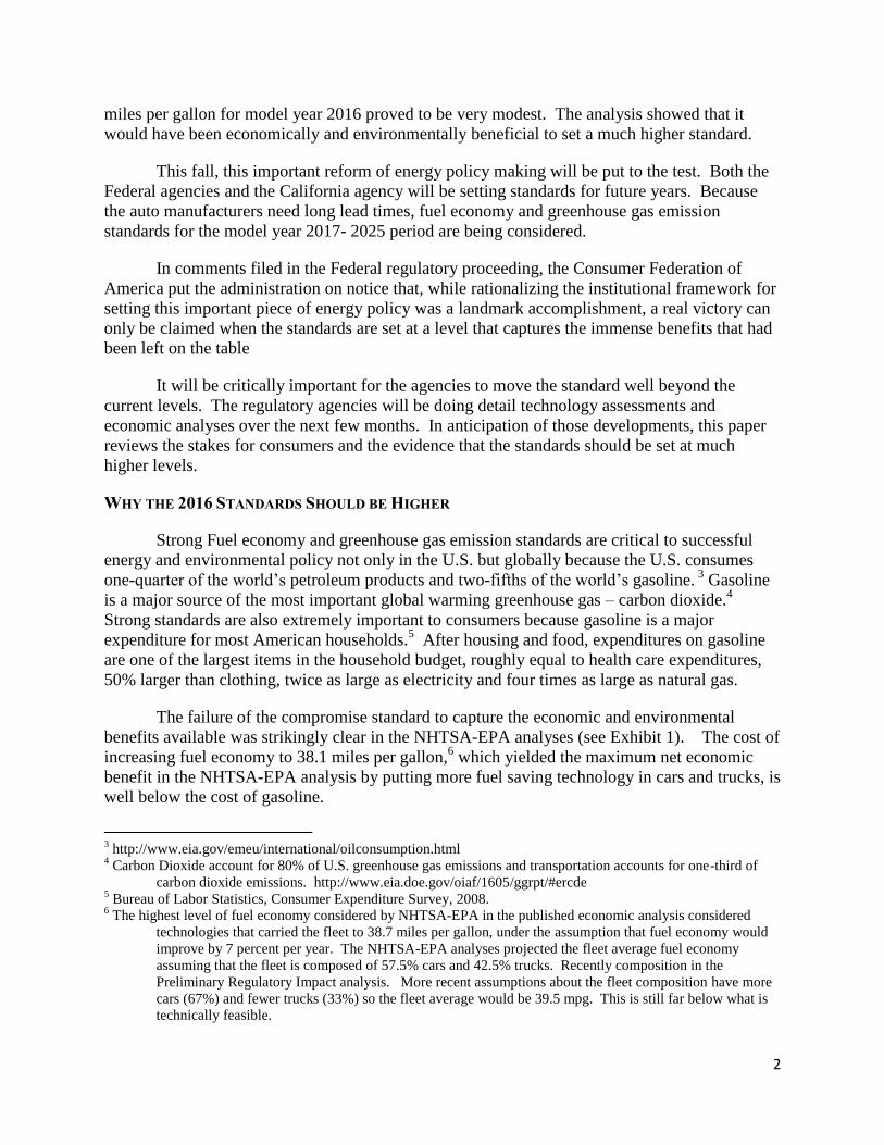
The failure of the compromise standard to capture the economic and environmental
benefits available was strikingly clear in the NHTSA-EPA analyses (see Exhibit 1). The cost of
increasing fuel economy to 38.1 miles per gallon,6 which yielded the maximum net economic
benefit in the NHTSA-EPA analysis by putting more fuel saving technology in cars and trucks, is
well below the cost of gasoline.
3 http://www.eia.gov/emeu/international/oilconsumption.html
4 Carbon Dioxide account for 80% of U.S. greenhouse gas emissions and transportation accounts for one-third of
carbon dioxide emissions. http://www.eia.doe.gov/oiaf/1605/ggrpt/#ercde 5 Bureau of Labor Statistics, Consumer Expenditure Survey, 2008.
6 The highest level of fuel economy considered by NHTSA-EPA in the published economic analysis considered
technologies that carried the fleet to 38.7 miles per gallon, under the assumption that fuel economy would
improve by 7 percent per year. The NHTSA-EPA analyses projected the fleet average fuel economy
assuming that the fleet is composed of 57.5% cars and 42.5% trucks. Recently composition in the
Preliminary Regulatory Impact analysis. More recent assumptions about the fleet composition have more
cars (67%) and fewer trucks (33%) so the fleet average would be 39.5 mpg. This is still far below what is
technically feasible.
3
EXHIBIT 1: ECONOMIC, NATIONAL SECURITY AND ENVIRONMENTAL BENEFITS OF VARIOUS
ALTERNATIVE STANDARD LEVELS
Conceptual MPG Economic Benefit National Security Cost per Environmental
Basis of the 2016 (Billion $, Net NPV) Reduced Gasoline gallon Greenhouse Gas
Standard Societal Consumer Consumption saved Reduction
Pocketbook (Billion Gallons) (Billion Tons)
Proposed 34.1 141 106 62 $0.98 29
Max. Environmental/ 38.1 191 143 95 $1.28 42
Economic Benefit
Sources and notes: National Highway Traffic Safety Administration and Environmental Protection Agency,
Proposed Rulemaking to Establish Light Duty Vehicle Greenhouse Gas Emission Standards and Corporate
Average Fuel Economy Standards. Preliminary Regulatory Impact Analysis, Tables 1b, 7, 8, 9, and 10. The 3
percent discount rate scenario is used. The consumer pocketbook calculation subtracts the cost of meeting
the standard (technology cost) from the fuel savings (lifetime fuel expenditures) and adds in the reduction in
the price of gasoline (the petroleum market externality). These are the direct, monetary impacts affecting
consumer pocketbooks. Fuel savings and market externalities are assumed to scale with the quantity of
gasoline consumption reduction.
The failure of the compromise standard to capture the economic and environmental
benefits available was strikingly clear in the NHTSA-EPA analyses (see Exhibit 1). The cost of
increasing fuel economy to 38.1 miles per gallon,7 which yielded the maximum net economic
benefit in the NHTSA-EPA analysis by putting more fuel saving technology in cars and trucks, is
well below the cost of gasoline.
At 38.1 mpg, it costs only $1.28 to save a gallon of gasoline, which is less than half
the current cost of gasoline of about $2.75, so consumers would end up saving almost
$1.50 on every gallon they buy.
Although the more fuel efficient vehicle would cost more, the increase in the
monthly loan payment to purchase at more fuel-efficient vehicle is less than
the reduction in expenditures for gasoline, making it cash flow positive from
the beginning, and the vehicle would have higher value at resale.
Setting fuel economy standards at the higher level helps to solve the nation’s
energy and environmental problems. It can reduce gasoline consumption by a
cumulative total of 95 billion gallons and yields consumer pocketbook savings
of over $140 billion, over the life of the vehicles covered by the standard.
Cumulative total societal benefits are over $190 billion while it reduces
greenhouse gas emissions by over 42 billion tons.
7 The highest level of fuel economy considered by NHTSA-EPA in the published economic analysis considered
technologies that carried the fleet to 38.7 miles per gallon, under the assumption that fuel economy would
improve by 7 percent per year. The NHTSA-EPA analyses projected the fleet average fuel economy
assuming that the fleet is composed of 57.5% cars and 42.5% trucks. More recent assumptions about the
fleet composition have more cars (67%) and fewer trucks (33%) so the fleet average would be 39.5 mpg.
This is still far below what is technically feasible.
4
TECHNOLOGY IS AVAILABLE FOR STANDARDS TO GO MUCH HIGHER
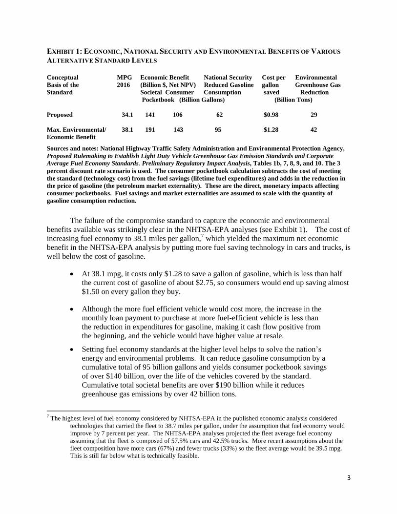
The highest levels of fuel economy that NHTSA-EPA considered for 2016 do not come
close to identifying the level of the standard that would be economically justified. As shown in
Exhibit 2, in the 2008 Corporate Average Fuel Economy (CAFE) proceeding, NHTSA examined
a potential standard it called Technology Exhaustion, which is the point where the maximum
usage of available technologies to reduce energy consumption is reached, disregarding the cost
impacts. Under that standard, the fuel economy for the fleet would have risen to approximately
45 miles per gallon by 2016.8
EXHIBIT 2: POTENTIAL FOR LONG TERM IMPROVEMENT IN FUEL ECONOMY STANDARDS
Sources and notes: National Highway Traffic Safety Administration and Environmental Protection, Agency,
Proposed Rulemaking to Establish Light Duty Vehicle Greenhouse Gas Emission Standards and Corporate
Average Fuel Economy Standards. Preliminary Regulatory Impact Analysis, Tables 1b; National Highway
Traffic Safety Administration, Average Fuel Economy Standards, Passenger Cars and Light Trucks,
Preliminary Regulatory Impact Analysis, 2008 Table 1b.
The technology exhaust limit is not fixed. The limit should advance over time as the cost
of technologies declines, the automakers become more adept at incorporating new technologies
and technologies move from the research and development phase into the deployment phase.
Using the regression line in Exhibit 2, projecting a constant rate of growth puts the technology
exhaust point at 60 mpg by 2020 and close to 90 mpg by 2030.
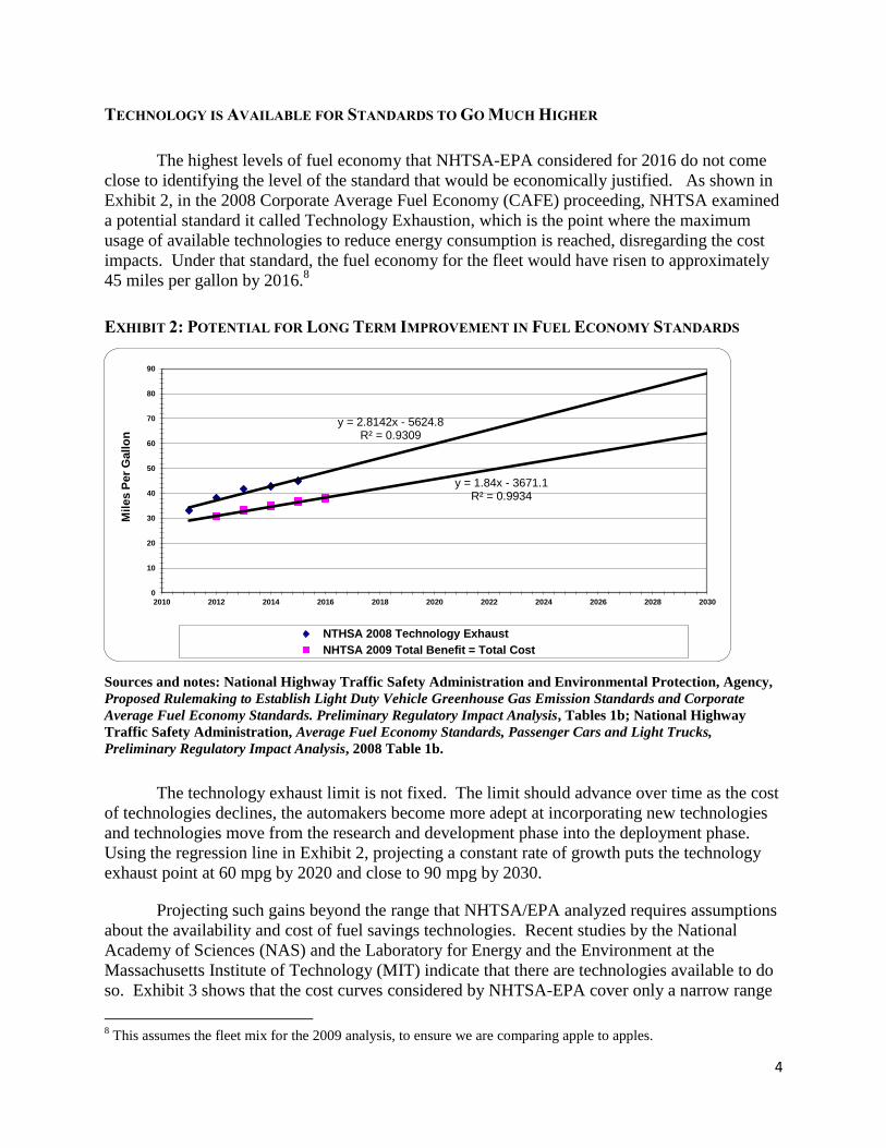
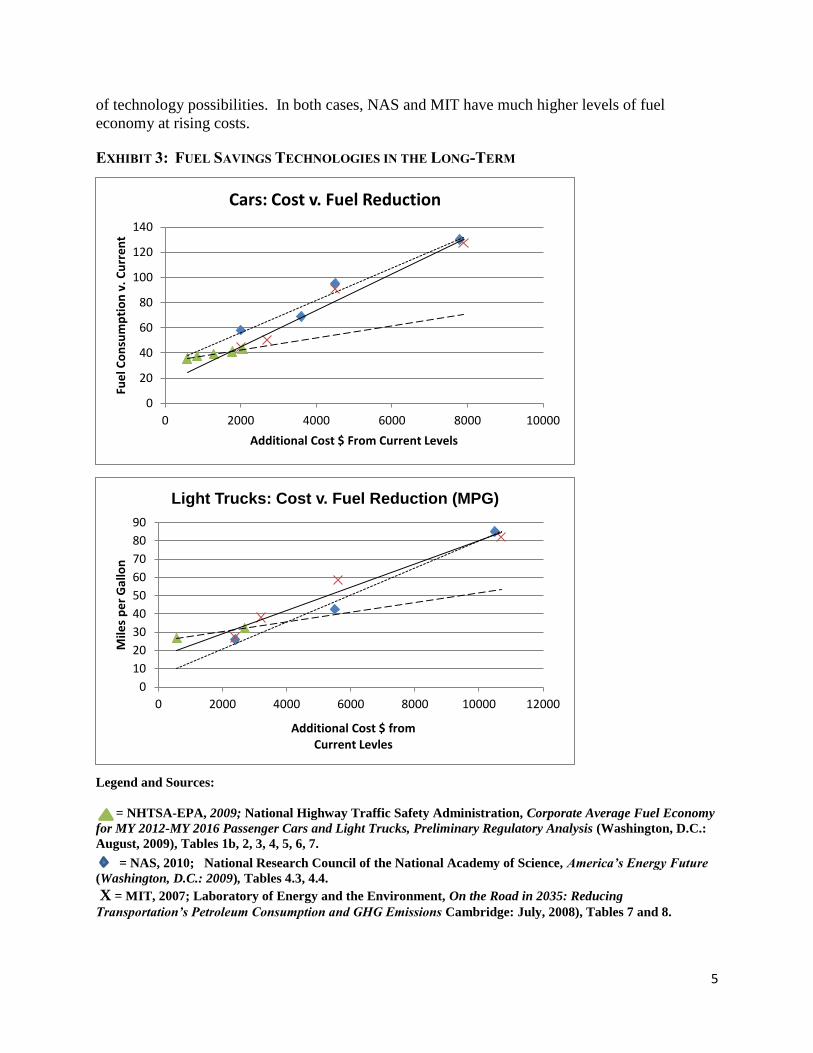
Projecting such gains beyond the range that NHTSA/EPA analyzed requires assumptions
about the availability and cost of fuel savings technologies. Recent studies by the National
Academy of Sciences (NAS) and the Laboratory for Energy and the Environment at the
Massachusetts Institute of Technology (MIT) indicate that there are technologies available to do
so. Exhibit 3 shows that the cost curves considered by NHTSA-EPA cover only a narrow range
8 This assumes the fleet mix for the 2009 analysis, to ensure we are comparing apple to apples.
y = 2.8142x - 5624.8 R² = 0.9309
y = 1.84x - 3671.1 R² = 0.9934
0
10
20
30
40
50
60
70
80
90
2010 2012 2014 2016 2018 2020 2022 2024 2026 2028 2030
Mil
es P
er
Gall
on
NTHSA 2008 Technology Exhaust
NHTSA 2009 Total Benefit = Total Cost
5
0
10
20
30
40
50
60
70
80
90
0 2000 4000 6000 8000 10000 12000
Mile
s p
er
Gal
lon
Additional Cost $ from Current Levles
Light Trucks: Cost v. Fuel Reduction (MPG)
0
20
40
60
80
100
120
140
0 2000 4000 6000 8000 10000
Fue
l Co
nsu
mp
tio
n v
. Cu
rre
nt
Additional Cost $ From Current Levels
Cars: Cost v. Fuel Reduction
of technology possibilities. In both cases, NAS and MIT have much higher levels of fuel
economy at rising costs.
EXHIBIT 3: FUEL SAVINGS TECHNOLOGIES IN THE LONG-TERM
Legend and Sources:
= NHTSA-EPA, 2009; National Highway Traffic Safety Administration, Corporate Average Fuel Economy
for MY 2012-MY 2016 Passenger Cars and Light Trucks, Preliminary Regulatory Analysis (Washington, D.C.:
August, 2009), Tables 1b, 2, 3, 4, 5, 6, 7.
= NAS, 2010; National Research Council of the National Academy of Science, America’s Energy Future
(Washington, D.C.: 2009), Tables 4.3, 4.4.
X = MIT, 2007; Laboratory of Energy and the Environment, On the Road in 2035: Reducing
Transportation’s Petroleum Consumption and GHG Emissions Cambridge: July, 2008), Tables 7 and 8.
6
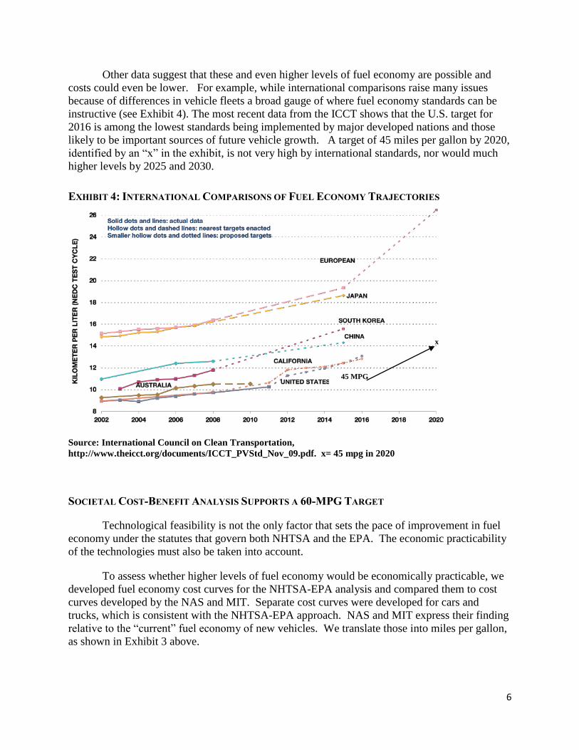
Other data suggest that these and even higher levels of fuel economy are possible and
costs could even be lower. For example, while international comparisons raise many issues
because of differences in vehicle fleets a broad gauge of where fuel economy standards can be
instructive (see Exhibit 4). The most recent data from the ICCT shows that the U.S. target for
2016 is among the lowest standards being implemented by major developed nations and those
likely to be important sources of future vehicle growth. A target of 45 miles per gallon by 2020,
identified by an “x” in the exhibit, is not very high by international standards, nor would much
higher levels by 2025 and 2030.
EXHIBIT 4: INTERNATIONAL COMPARISONS OF FUEL ECONOMY TRAJECTORIES
x
45 MPG
Source: International Council on Clean Transportation,
http://www.theicct.org/documents/ICCT_PVStd_Nov_09.pdf. x= 45 mpg in 2020
SOCIETAL COST-BENEFIT ANALYSIS SUPPORTS A 60-MPG TARGET
Technological feasibility is not the only factor that sets the pace of improvement in fuel
economy under the statutes that govern both NHTSA and the EPA. The economic practicability
of the technologies must also be taken into account.
To assess whether higher levels of fuel economy would be economically practicable, we
developed fuel economy cost curves for the NHTSA-EPA analysis and compared them to cost
curves developed by the NAS and MIT. Separate cost curves were developed for cars and
trucks, which is consistent with the NHTSA-EPA approach. NAS and MIT express their finding
relative to the “current” fuel economy of new vehicles. We translate those into miles per gallon,
as shown in Exhibit 3 above.
7
-4
-3
-2
-1
0
1
2
3
4
5
0 1000 2000 3000 4000 5000 6000 7000 8000
Fue
l Co
nsu
mp
tio
n v
. Cu
rre
nt/
B
be
ne
fit-
Co
st R
atio
Additional Cost
Cars: Cost v. Fuel Reduction & Cost Benefit Ratio
0
20
40
60
80
100
120
140
0 1000 2000 3000 4000 5000 6000 7000 8000
Fue
l Co
nsu
mp
tio
n v
. Cu
rre
nt
Additional Cost
Cars: Cost v. Fuel Reduction
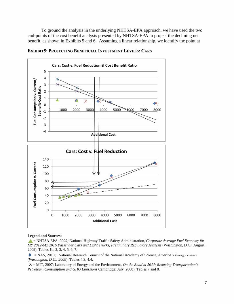
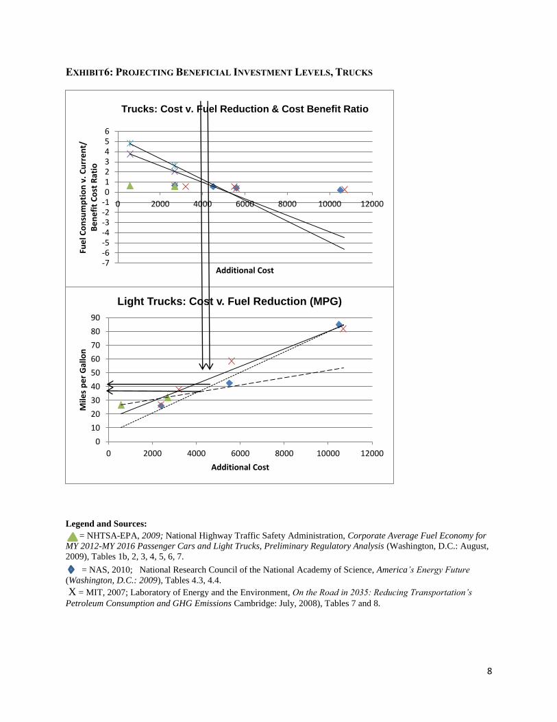
To ground the analysis in the underlying NHTSA-EPA approach, we have used the two
end-points of the cost benefit analysis presented by NHTSA-EPA to project the declining net
benefit, as shown in Exhibits 5 and 6. Assuming a linear relationship, we identify the point at
EXHIBIT5: PROJECTING BENEFICIAL INVESTMENT LEVELS: CARS
Legend and Sources:
= NHTSA-EPA, 2009; National Highway Traffic Safety Administration, Corporate Average Fuel Economy for
MY 2012-MY 2016 Passenger Cars and Light Trucks, Preliminary Regulatory Analysis (Washington, D.C.: August,
2009), Tables 1b, 2, 3, 4, 5, 6, 7.
= NAS, 2010; National Research Council of the National Academy of Science, America’s Energy Future
(Washington, D.C.: 2009), Tables 4.3, 4.4.
X = MIT, 2007; Laboratory of Energy and the Environment, On the Road in 2035: Reducing Transportation’s
Petroleum Consumption and GHG Emissions Cambridge: July, 2008), Tables 7 and 8.
8
-7-6-5-4-3-2-10123456
0 2000 4000 6000 8000 10000 12000
Fue
l Co
nsu
mp
tio
n v
. Cu
rre
nt/
B
en
efi
t C
ost
Rat
io
Additional Cost
Trucks: Cost v. Fuel Reduction & Cost Benefit Ratio
0
10
20
30
40
50
60
70
80
90
0 2000 4000 6000 8000 10000 12000
Mile
s p
er
Gal
lon
Additional Cost
Light Trucks: Cost v. Fuel Reduction (MPG)
EXHIBIT6: PROJECTING BENEFICIAL INVESTMENT LEVELS, TRUCKS
Legend and Sources:
= NHTSA-EPA, 2009; National Highway Traffic Safety Administration, Corporate Average Fuel Economy for
MY 2012-MY 2016 Passenger Cars and Light Trucks, Preliminary Regulatory Analysis (Washington, D.C.: August,
2009), Tables 1b, 2, 3, 4, 5, 6, 7.
= NAS, 2010; National Research Council of the National Academy of Science, America’s Energy Future
(Washington, D.C.: 2009), Tables 4.3, 4.4.
X = MIT, 2007; Laboratory of Energy and the Environment, On the Road in 2035: Reducing Transportation’s
Petroleum Consumption and GHG Emissions Cambridge: July, 2008), Tables 7 and 8.
9
which the benefit cost ratio equals one and calculate the amount of investment that would occur
at that point. This is the point on the technology cost curve where total benefit equals cost. We
then estimate the fuel economy that would be achieved by that level of investment on the MIT
and NAS regression lines.9
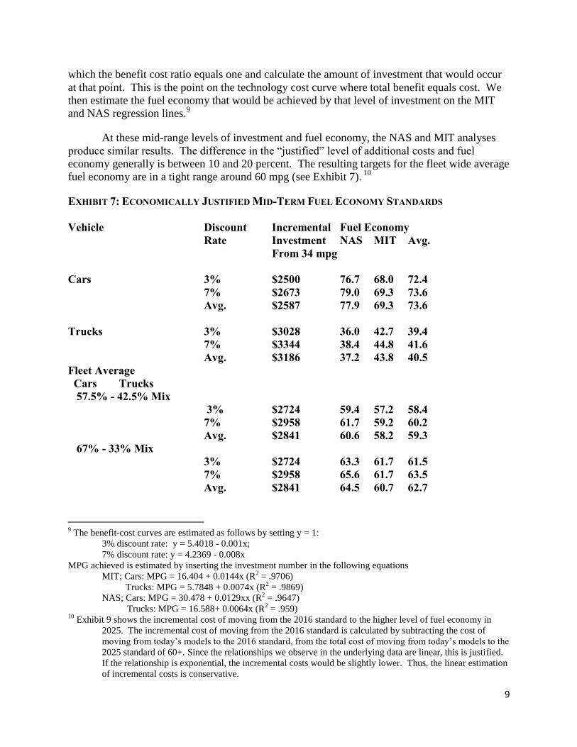
At these mid-range levels of investment and fuel economy, the NAS and MIT analyses
produce similar results. The difference in the “justified” level of additional costs and fuel
economy generally is between 10 and 20 percent. The resulting targets for the fleet wide average
fuel economy are in a tight range around 60 mpg (see Exhibit 7). 10
EXHIBIT 7: ECONOMICALLY JUSTIFIED MID-TERM FUEL ECONOMY STANDARDS
Vehicle Discount Incremental Fuel Economy
Rate Investment NAS MIT Avg.
From 34 mpg
Cars 3% $2500 76.7 68.0 72.4
7% $2673 79.0 69.3 73.6
Avg. $2587 77.9 69.3 73.6
Trucks 3% $3028 36.0 42.7 39.4
7% $3344 38.4 44.8 41.6
Avg. $3186 37.2 43.8 40.5
Fleet Average
Cars Trucks
57.5% - 42.5% Mix
3% $2724 59.4 57.2 58.4
7% $2958 61.7 59.2 60.2
Avg. $2841 60.6 58.2 59.3
67% - 33% Mix
3% $2724 63.3 61.7 61.5
7% $2958 65.6 61.7 63.5
Avg. $2841 64.5 60.7 62.7
9 The benefit-cost curves are estimated as follows by setting y = 1:
3% discount rate: y = 5.4018 - 0.001x;
7% discount rate: y = 4.2369 - 0.008x
MPG achieved is estimated by inserting the investment number in the following equations
MIT; Cars: MPG = 16.404 + 0.0144x (R2 = .9706)
Trucks: MPG = 5.7848 + 0.0074x (R2 = .9869)
NAS; Cars: MPG = 30.478 + 0.0129xx (R2 = .9647)
Trucks: MPG = 16.588+ 0.0064x (R2 = .959)
10 Exhibit 9 shows the incremental cost of moving from the 2016 standard to the higher level of fuel economy in
2025. The incremental cost of moving from the 2016 standard is calculated by subtracting the cost of
moving from today’s models to the 2016 standard, from the total cost of moving from today’s models to the
2025 standard of 60+. Since the relationships we observe in the underlying data are linear, this is justified.
If the relationship is exponential, the incremental costs would be slightly lower. Thus, the linear estimation
of incremental costs is conservative.
10
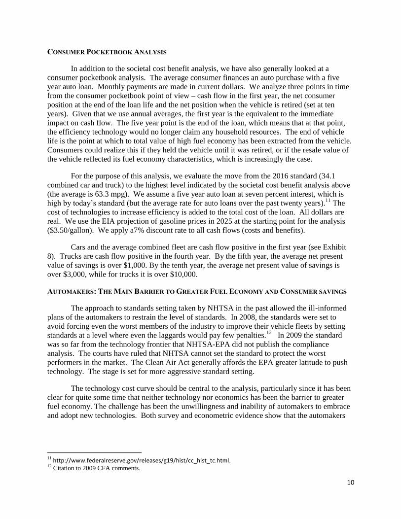
CONSUMER POCKETBOOK ANALYSIS
In addition to the societal cost benefit analysis, we have also generally looked at a
consumer pocketbook analysis. The average consumer finances an auto purchase with a five
year auto loan. Monthly payments are made in current dollars. We analyze three points in time
from the consumer pocketbook point of view – cash flow in the first year, the net consumer
position at the end of the loan life and the net position when the vehicle is retired (set at ten
years). Given that we use annual averages, the first year is the equivalent to the immediate
impact on cash flow. The five year point is the end of the loan, which means that at that point,
the efficiency technology would no longer claim any household resources. The end of vehicle
life is the point at which to total value of high fuel economy has been extracted from the vehicle.
Consumers could realize this if they held the vehicle until it was retired, or if the resale value of
the vehicle reflected its fuel economy characteristics, which is increasingly the case.
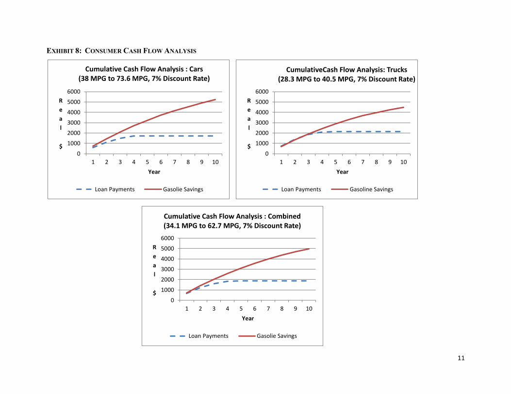
For the purpose of this analysis, we evaluate the move from the 2016 standard (34.1
combined car and truck) to the highest level indicated by the societal cost benefit analysis above
(the average is 63.3 mpg). We assume a five year auto loan at seven percent interest, which is
high by today’s standard (but the average rate for auto loans over the past twenty years).11
The
cost of technologies to increase efficiency is added to the total cost of the loan. All dollars are
real. We use the EIA projection of gasoline prices in 2025 at the starting point for the analysis
($3.50/gallon). We apply a7% discount rate to all cash flows (costs and benefits).
Cars and the average combined fleet are cash flow positive in the first year (see Exhibit
8). Trucks are cash flow positive in the fourth year. By the fifth year, the average net present
value of savings is over $1,000. By the tenth year, the average net present value of savings is
over $3,000, while for trucks it is over $10,000.
AUTOMAKERS: THE MAIN BARRIER TO GREATER FUEL ECONOMY AND CONSUMER SAVINGS
The approach to standards setting taken by NHTSA in the past allowed the ill-informed
plans of the automakers to restrain the level of standards. In 2008, the standards were set to
avoid forcing even the worst members of the industry to improve their vehicle fleets by setting
standards at a level where even the laggards would pay few penalties.12
In 2009 the standard
was so far from the technology frontier that NHTSA-EPA did not publish the compliance
analysis. The courts have ruled that NHTSA cannot set the standard to protect the worst
performers in the market. The Clean Air Act generally affords the EPA greater latitude to push
technology. The stage is set for more aggressive standard setting.
The technology cost curve should be central to the analysis, particularly since it has been
clear for quite some time that neither technology nor economics has been the barrier to greater
fuel economy. The challenge has been the unwillingness and inability of automakers to embrace
and adopt new technologies. Both survey and econometric evidence show that the automakers
11
http://www.federalreserve.gov/releases/g19/hist/cc_hist_tc.html. 12
Citation to 2009 CFA comments.
11
0
1000
2000
3000
4000
5000
6000
1 2 3 4 5 6 7 8 9 10
R
e
a
l
$
Year
Cumulative Cash Flow Analysis : Combined (34.1 MPG to 62.7 MPG, 7% Discount Rate)
Loan Payments Gasolie Savings
0
1000
2000
3000
4000
5000
6000
1 2 3 4 5 6 7 8 9 10
R
e
a
l
$
Year
Cumulative Cash Flow Analysis : Cars (38 MPG to 73.6 MPG, 7% Discount Rate)
Loan Payments Gasolie Savings
0
1000
2000
3000
4000
5000
6000
1 2 3 4 5 6 7 8 9 10
R
e
a
l
$
Year
CumulativeCash Flow Analysis: Trucks (28.3 MPG to 40.5 MPG, 7% Discount Rate)
Loan Payments Gasoline Savings
EXHIBIT 8: CONSUMER CASH FLOW ANALYSIS
12
failed to react to clear shifts in consumer preferences, which contributed to their severe
difficulties.13
The technology cost curves used in this analysis are defined as long-term, 2035, but the
analysis in this paper focuses on standards to be set in 2025. The acceleration of a decade could
be a challenge for the industry, but the technologies that underlay the cost curves are already in
the vehicle fleet to some extent, or close to being in the fleet. Setting a high standard for a
decade and a half in the future can push the industry to be more innovative and responsive to
consumer demand, as well as national energy and environmental needs and goals. Coordinating
between the three agencies with authority to set standards (CARB, EPA and NHTSA) and
preserving California’s important role in maintaining momentum were important procedural
steps to progress, now it is vital to move the standards to the much higher levels that the
consumer pocketbook and societal cost benefit analysis support.
13
Cooper, Mark, U.S. Oil Markets Fundamentals and Public Opinion (Consumer Fedeationof America, May 2010);
Ending America’s Oil Addiction (Consumer Federation of America, April 2008.