SGEMS-UQ: An Uncertainty Quantification Toolkit for

SGEMS

Lewis Li1, Alexandre Boucher2 and Jef Caers3 1Electrical Engineering Department, Stanford University, USA 2Advanced Resources and Risk Technology, USA 3Energy Resources Engineering department, Stanford University, USA

Abstract

While algorithms and methodologies to study uncertainty in the Earth Sciences are constantly

evolving, there are currently few open-source integrated softwares that allows the general

practitioners access to these developments. This paper presents SGEMS-UQ, a plugin for the

SGEMS platform, that is used to perform distance-based uncertainty analysis on geostatistical

simulations, and the resulting transfer functions responses used in subsurface modeling and

engineering. A versatile XML-derived dialect is defined for communicating with external

programs that eliminates the need for ad-hoc linking of codes, and a relational database system

is implemented to automate many of the steps in data mining the spatial and forward model

parameters. Through a graphical user interface, one can map a set of realizations and transfer

function responses into a multidimensional scaling (MDS) space where advanced visualization

utilities, and clustering techniques are available. Once mapped in the MDS space, the user can

explore linkage between parameters and transfer function responses by querying a SQL

database. Consideration is given to the use of programming designs to produce a code-base

that is manageable, efficient, and extensible for future applications, while being scalable to

work with large datasets. Finally, we illustrate the versatility of the code-base on a real-field

application of modeling uncertainty in reservoir forecasts for an Oil reservoir of the West Coast

of Africa.

Keywords: uncertainty quantification, software design, XML, SQL database

Introduction

With an increase in modeling and computational methodologies, codes and hardware

resources, the aspect of uncertainty has received increased attention in the Earth Sciences (e.g.

Wu, et al., 2006; Brown and Heuvelink, 2007; Caers, 2011). In this paper we focus on

uncertainty problems that involve geostatistical modeling (Chilles and Delfiner 1999) and

computationally demanding transfer functions for which these geostatistical models are

created. The example applications targeted in this paper are mostly related to subsurface

modeling and engineering (e.g. modeling of groundwater systems, conventional and

unconventional energy resources, mining and CO2 sequestration), but the resulting software,

SGEMS-UQ, could be applied to any other similar applications. In terms of modeling and

decision-making, a possible workflow is outlined in Figure 1, adapted from Caers (2011). The

geological scenarios are built with a number of geostatistical algorithms, either covariance-

based (Chilles and Delfiner 1999), Boolean (Holden, et al. 1998) or multiple-point statistics

(Caers and Zhang, 2004; Mariethoz, et al., 2009, Strebelle 2002). Each algorithm has parameters

such as mean, variance, covariance, training image, object shapes and dimensions that are

uncertain and need to be varied. In terms of software, several packages, commercial and open-

source are available for geostatistical studies. The development of this uncertainty module is a

plug-in to SGEMS (Stanford Geostatistical Earth Modeling software, sgsems.sourceforge.net).

Geostatistical modeling is generally fast in terms of CPU with algorithms from covariance or

training image being parallelized (Peredo and Ortiz 2011), that run million-cell grid in seconds

or minutes. However, within the described applications, geostatistical modeling is rarely an

end-goal, and the resulting models are then typically used for evaluating flow, geo-mechanical

or geophysical (seismic, EM, GPR) equations, including the coupling of these equations.

Software such as TOUGH (Lawrence Berkeley National Laboratory, 2012) and MODFLOW

(Harbaugh 2005) require hours to days of computational effort. Other evaluations consider

optimization codes such as the optimization of open-pit design in mining (e.g. Dimitrakopoulos

and Ramazan, 2004).

Modern software engineering relies on concepts of re-usability, extensibility and

maintainability of the design, which our software targets as well. Commercial platforms such as

Ocean/Petrel (Schlumberger Limited 2010) aim at providing such capabilities, but no open-

source codes combine the full capabilities of geostatistical modeling with forward modeling or

optimization codes. While most researchers write codes that link the various components

described in Figure 1, these codes are linked in an ad-hoc fashion, often with simple scripting or

MATLAB, and are neither re-useable nor extensible. These codes need then to be rewritten

(and compiled) for every different application or set of input parameters. Then there is the

problem of data management in real field applications. Many components of the workflow in

Figure 1 can be randomized; hence possibly hundreds of geostatistical models may be created

to capture uncertainty within such set of geostatistical models. After evaluating forward

equations on the geostatistical models, there is often a need to post-process the results. For

example, a sensitivity analysis is performed attempting to discover which parameters or

combinations of parameters have the largest impact on the responses. A visualization of the

uncertainty spanned by the responses is performed using dimensionality reduction and data

mining techniques such as multi-dimensional scaling (MDS) (Honarkhah, 2009), support vector

machines (SVM) (Cortes, 1995) or various forms of principle component analysis (PCA) (Abdi,

2010).

In this paper we address the software challenges by defining a versatile XML-derived dialect for

communicating with external programs that eliminates the need for ad-hoc linking of codes,

and the implementation of a relational database system that automates many of the steps in

data mining the spatial and forward model parameters. Consideration is given to the use of

programming designs to produce a code-base that is manageable, efficient, and extensible for

future applications, while being scalable to work with large datasets. Our methodology for

modeling uncertainty within this framework relies on the concept of distance-based modeling

of uncertainty (Caers, 2011; Caers et al., 2011; Scheidt and Caers, 2009a, 2009b), but the

presented design could be extended to other types of approaches. After reviewing the main

concepts of the distance-based uncertainty modeling workflow, we present our software design

to handle the dual challenge of coupling codes and managing the information generated by the

Monte Carlo approach of the method. Finally, we present a real-field application of modeling

uncertainty in reservoir forecasts for an Oil reservoir of the West Coast of Africa.

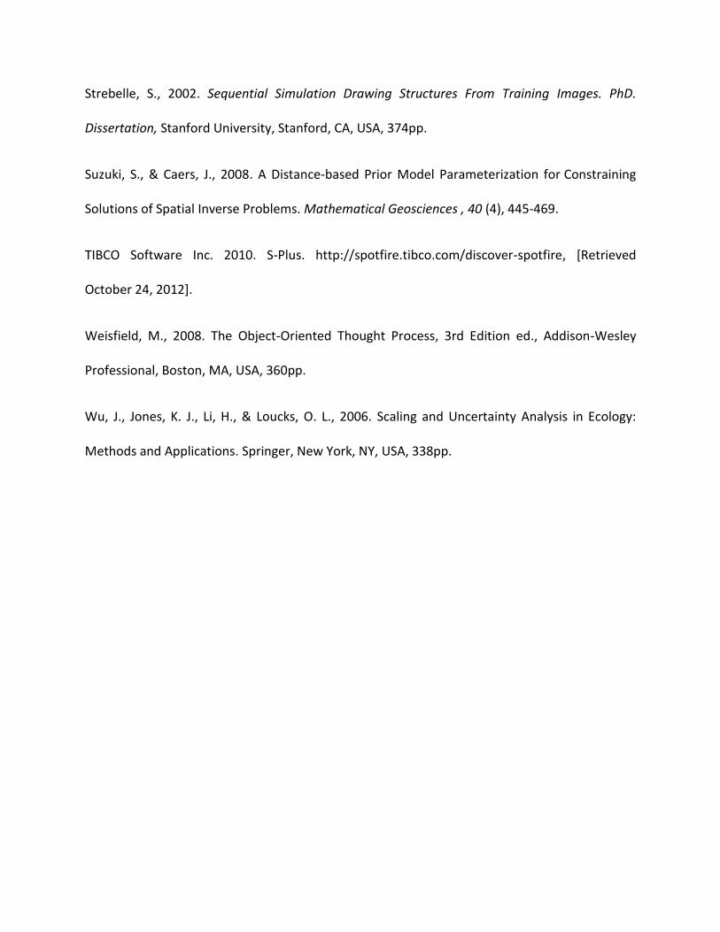
Review of Distance-Based Modeling of Uncertainty

The contribution of this paper lies in the software design for modeling uncertainty using

geostatistical simulation methods and computationally demanding forward modeling codes.

This section reviews the distance-based approach for modeling uncertainty that was

implemented in the software. Other approaches use experimental design; response surface

modeling could follow a similar software design since they call on similar basic elements of such

analysis: geostatistical codes, forward modeling codes and post-processing of the runs. The

challenge lies in linking codes and managing the information generated by such modeling

frameworks.

The main contribution of distance-based uncertainty quantification is to recognize that often a

more efficient and effective quantification of variation is that by means of distances, as

opposed to for example, variances and covariance. Distances and kernels are commonly used in

computer science (Liu, 2010). In our applications, we recognize that differences (distances) in

response variables can be used to quantify uncertainty. The distance-based approach is

summarized in Figure 2 (adapted from Caers (2011)) and consists of a number of steps:

1. A prior uncertainty is stated (from actual data) on spatial and forward model

parameters. Either experimental design or Monte Carlo simulation is used to generate

sets of input parameters. Some parameters may be continuous (e.g. a mean) other

discrete (e.g. a rock-type) or scenario-based (e.g. a geological interpretation).

2. A geostatistical algorithm is used to generate realizations. A few models are shown in

Figure 2.

3. A distance is defined between the realizations. This distance can be based directly on

the realizations (a static distance) or could involve an approximate physical model

(surrogate or proxy model). These static or dynamic proxies are needed when the full

forward model is too computationally expensive.

4. Multi-dimensional-scaling (MDS) is used to map the realization into a low dimensional

space for visualization purposes. MDS is basically a dimensionality reduction technique

based on the dot-product (Honarkhah and Caers, 2010 for a geostatistical application of

MDS).

5. A clustering algorithm is applied to group models into a set of distinct clusters. Figure 3

shows that such clustering can be a k-medoid or a kernel k-medoid clustering. The k-

medoid selects one of the models as a cluster representative.

6. The full physics forward model is now applied to selected models to represent the

response uncertainty

7. Analysis of the information generated from step 1 to 6: distances, parameters per

cluster, selected models, quantiles of response uncertainty and more.

Any software design for uncertainty quantification will require some flexibility in

What parameters are specified and how their prior uncertainty is modeled

What geostatistical algorithms (or combinations) are used

What proxy models are used: static, dynamic or combinations

How distances are calculated

What the full physics forward models are

How users want to analysis the results and/or do sensitivity analysis

In the next section we present a program design that addresses these challenges.

Software Design

Coupling with existing SGEMS codebase

The main SGEMS program provides the input parameters, geostatistical algorithms and their

results, while dynamic simulators are considered external codes. The decision to integrate the

uncertainty toolkit with SGEMS has the advantage of having access to the source code,

standards and conventions used by SGEMS, which are open source. The main SGEMS software

was written using the Qt4 framework with external dependencies on VTK (Schroeder, Martin

and Loresen 2004), Eigen3 (Guennebaud, Jacob and et al. 2010), and Boost (Karlsson 2005). It

has been successfully compiled and used on Windows, OSX and Linux. By developing SGEMS-

UQ as a plugin to SGEMS, as opposed to a standalone program, much of SGEMS’ codebase can

be reused; most notably loading/saving project files, and visualizing any generated

geostatistical models. SGEMS has the capability to use multiple algorithms to generate models

with the resulting models following a standard format and convention. This means that by

catering to this single specified convention, SGEMS-UQ is guaranteed to be extensible to any

future geostatistical algorithms that may be added to SGEMS.

SGEMS follows a factory method design pattern for its plugins (Fowler, et al. 1999), which

defines an interface for creating plugin classes, but the class must instantiate itself. This

paradigm allows for the SGEMS main program to take over the lifetime management of the

SGEMS-UQ plugin, reducing code duplication. Plugins use the Qt .ui file specification to define

the user interface for the plugin. This means Qt Designer program can be used as an editor for

developing the plugin GUI, allowing for the preservation of visual styles with the main SGEMS

program. However, SGEMS-UQ contains substantially more components than existing SGEMS

plugins. As shown in Figure 4, SGEMS-UQ is comprised of three separate modules. The first is

SGEMS-Metrics, which allows contains the filters required to load responses from third party

simulators. GSTL_item_model contains the framework used to compute and store the MDS

space, in addition to providing an interface to store simulation parameters to an external

database. The final MDS-GUI provides capabilities such as multiple visualizers, clustering and

sensitivity analysis. This increase in software complexity makes the use of an effective

programing design crucial in preventing code bloat, and encouraging extensibility, re-usability,

and maintenance of the codebase.

A motivating factor behind the software design of SGEMS-UQ is the efficient visualization of

multiple forms of data. SGEMS-UQ uses the Model-View-Controller (MVC) programming design

(Weisfield 2008) to display the subsets of data across different views without requiring each

visualizer to have its own copy of the same data. The basic premise of MVC revolves around

abstracting the various aspects of the program into the three constituent components of the

namesake. The model contains the data that is used by the entire program. In SGEMS-UQ, the

models consist of the response variables, MDS spaces, and input parameters. The view is the

visualizer of the models, which in SGEMS-UQ manifests as VTK plots (Schroeder, Martin and

Loresen 2004) of the various variables. The controller defines the method in which the user

interacts with the model. Plotting subsets of response variables or common parameters over

different clusters are all examples where the same model data needs to be displayed over

multiple views. MVC allows SGEMS-UQ to keep only a single copy of the response variables

despite numerous visualization windows.

While SGEMS is used to generate models, external programs are used to generate the response

variables required for performing distance-based uncertainty modeling. This necessitates a

method of importing data from external simulators into SGEMS-UQ. Presently, most dynamic

simulators output the simulation results into space delimited or comma separated values (for

example Eclipse (Schlumberger Limited 2010), Modflow (Harbaugh 2005), TOUGH (Lawrence

Berkeley National Laboratory, 2012)). To address the import of data from external programs,

SGEMS-UQ uses a specified XML dialect to transfer data between processes. While the choice

of XML over a flat file is not superior in terms of reading speed, the extensibility of XML makes

it a more appropriate selection in this application since XML allows for the storage of both data

and structure information within the same file.

At this moment, SGEMS-UQ has the built-in capability to handle four response data format:

scalar, vector, time series and distribution. Each data response format has a distance function

associated with it. For instance the distance between two distributions is calculated differently

than between two scalars. This allows SGEMS-UQ to process arbitrary number of response data

(i.e. well pressure, cumulative water production, etc.), as long as they fall into an implemented

data category type. This drastically reduces overhead when compared to recompiling code for

each set of input parameters. Note that SGEMS-UQ is not restricted to these response data

format and a developer could add more formats that would automatically integrate with the

software infrastructure. Furthermore, the Qt framework provides standard functions to

process XML syntax.

Information management using an SQL database

Another requirement of SGEMS-UQ is to data mine the parameters in order to perform

sensitivity analysis and to better understand linkage between parameters and responses.

SGEMS-UQ follows the XML SGEMS convention for storing the simulation parameters for each

realization. The XML format accounting for the hierarchical nature of geostatistical parameters

(e.g. maximum range of a spherical variogram) and those parameters are not homogenous

across algorithms (Boolean versus Gaussian versus MPS). While XML is natively readable by

users, it is not an ideal format for displaying on a GUI, nor is it an appropriate database on

which searches can be performed. SGEMS-UQ converts the simulation parameters into two

different formats, each geared towards a specific purpose. The first one is to visualize the

parameters in a tree display format (Figure 10). The tree model viewer allows users the

capability to expand and collapse groups, providing a cleaner interface for reading an otherwise

convoluted list of parameters. Secondly, SGEMS-UQ parses the parameters from the XML

format into a SQL database (Date and Darwen 1996) for data mining. The specific database that

is used is SQLite, a database system designed to be small (275 kb), such that it can be shipped

as part of the client application. SQLite is ACID-compliant and is compatible with the majority of

the functions in the SQL (Owens 2006). In SGEMS-UQ, the database is embedded in local

memory, but the web-centric nature of the SQL standard can allow for storage on a central

server while clients connect in remotely. SQL is also highly scalable, which means that SGEMS-

UQ can be used to data mine thousands of realizations. Since SQL is a relational database,

SGEMS-UQ can directly insert and retrieve any information without worrying about the

underlying data structures and retrieval procedures to answer queries. Extensions could take

advantage of full suite SQL packages such as SQL Server that offers built in statistical packages

such as SPSS (IBM Corporation, 2012), SAS (SAS Institute, 2011), and S-Plus (TIBCO Software

Incorporated, 2010) for performing more complicated data mining operations.

The different nature of parameters (e.g. float versus string) adds an additional challenge to the

data-mining process. SGEMS-UQ automatically identifies the data type of each parameter and

provides associated comparison operators. For instance, string-based parameters can only be

matched exactly using string operators, while floating point parameters can be compared using

a variety of operators, such as less than, equal to, greater than, etc. By taking advantage of the

transform iterator and binary function predicates in the C++ Standard Template Library

(Musser, Derge and Saini 2001) released as part of the latest version C++11 (Becker 2008), this

query can be extended to searching across multiple parameters. For instance, finding all

realizations with both mean porosity less than 30 and variogram radius greater than 15.

Another example is to take a series of realizations and finds their common input parameters.

While a third operation considers each cluster generated from the k-medoid step, and

evaluates which parameters types are common to all realizations (realizations generated by

different algorithms can also be compared using this technique as long as they have

comparable parameters with the same name). The entire parameter explorer module is built on

top of two abstract classes; a database interface class (param_base_class) used to query the

system, and a visualizer class (param_plot_window) that allows for data to be plotted (Figure

5). This reduces code redundancy for derived classes, and facilitates the implementation of

future data mining operations.

SGEMS-UQ provides a cohesive and efficient workflow for performing distance-based

uncertainty quantification, as will be shown with a walkthrough example in the following

section.

Application and Example Usage

Case Study

In this section, SGEMS-UQ is demonstrated for a problem of uncertainty quantification in

production forecasts for a reservoir in West Coast Africa (termed WCA). WCA is a deep-water

turbidite offshore reservoir that was successfully analyzed using distance-based uncertainty

modeling in Scheidt and Caers (2009b) and Caers (2011). To account for the depositional

uncertainty, the SGEMS Training-image generator (Boucher 2010) algorithm was used to

generate training images, each representing a geological interpretation of the reservoir

depositional system. Facies realizations are then filled with porosity and permeability values

using traditional variogram-based techniques.

This MDS analysis case study requires multiple geostatistical algorithms and external proxy

simulators as well as full-physics simulators. Scheidt and Caers (2009a) used multiple MATLAB

and Python scripts to perform this analysis. SGEMS-UQ drastically simplifies the uncertainty

quantification workflow, in addition to providing previously unavailable capabilities in analyzing

the results. All code and data are available from http://github.com/SCRFpublic/SGEMS-UQ. The

complete analysis and runs are also provided on this page.

Uncertainty Model for WCA

The response variables used for the WDA case study are cumulative oil and water production,

both of which are time series data types. The computation of oil/water production requires a

set of porosity / permeability realizations. These realizations are generated in two steps. First,

the facies models (Figure 6) is generated using a Single Normal Equation Sequential Simulation

(Strebelle 2002) algorithm (SGEMS program snesim), constrained to well data and

corresponding 3D training image with properties delineated in Table 1. Then the porosity is

generated with the Sequential Gaussian Simulation (SGEMS program sgsim). A histogram of the

distribution of each facies type was extracted from the well data, and used as the target

histogram. Uncertainty in this histogram is modeled through a triangular distribution for mean

and variance (see Table 2 and Table 3).

The permeability values were generated with a Markov Model 1 collocated coregionalization

(Journel, 1999) (SGEMS program cosgsim) with the previously generated porosity values as the

soft data. The spatial distribution of porosity and permeability is simulated independently for

each facies. The porosity, permeability and facies are combined using a cookie cutter approach

using a Python script included in the aforementioned repository. For this particular example, 10

facies models were generated per training image, and 10 porosity/permeability maps for each

facies were created, resulting in 100 realizations per training image. The final resulting

realizations contain parameters from a series of four permeability and porosity maps; one for

each facies. A simple Python script is used gather the sets of parameter files from different

simulations into a single XML file that can be read by SGEMS-UQ. This script

(ParseParameters.py) can be used to group arbitrary sets of simulation parameters, allowing

SGEMS-UQ to be extensible to a wide variety of cases.

Interfacing With Third Party Simulators

The cumulative oil and water production was simulated using ECLIPSE, and exported to a space

delimited text file, where each column corresponds to a response variable, and each row is a

realization. This format can be converted into an appropriate XML file with a simple Python

script (parseResponse.py). This script was developed such that it can be modified or extended

to extract arbitrary data from different simulators into the standard SGEMS-UQ XML dialect.

SGEMS-UQ has the capability to plot varying types of response data, allowing the user to

visualize the amount of uncertainty represented by a set of realizations. Figure 8 shows an

example of a time series response.

Distance-Based Workflow

The following section demonstrates a step-by-step approach for the distance-based uncertainty

analysis study of WCA using SGEMS-UQ. Such steps would be typical to most data sets.

1. Generation of a MDS Space:

This step consists of selecting the realizations and proxy responses to be analyzed. Figure 8

shows the GUI used to specify the generation of the MDS space. Any subset of realizations and

proxy responses can be selected, and several MDS spaces can be independently created.

SGEMS-UQ only displays the proxy responses that are common to selected realizations, which

in turn corresponds to which distances can be used for the MDS calculation. The distances

themselves can be computed using a variety of distance kernels, selectable within the same

window. These kernels can be applied to any of the implemented data types, but additional

kernels can also be added for future extensibility.

2. Visualization of the MDS space:

Once the MDS space is created and loaded into the visualizer, 3D cloud of points can be viewed,

span, zoom and rotated. This gives the user a visual representation of the distances between

realizations with regards to their proxy responses. An example of which is shown in Figure 10.

Individual realizations can be selected with appropriate highlighting.

3. K-Medoid Clustering:

The realizations can then be clustered using the kernel k-medoid (KKM) algorithm, as shown in

Figure 9. The number of clusters is left as an input parameter and all clustering results are

stored within the program for further visualization or analysis; such as clusters highlighting in

the MDS space. The clustering can be repeated with several numbers of medoids, and all the

clusters are kept and saved along with the MDS space. Then, the selected medoid realizations,

assumed to be representative of their respective cluster, are exported to a text file. They can

then be put through full physics flow simulators. For this particular example, twelve medoids

were selected, and the P10, P50 and P90 responses for cumulative oil and water production are

shown along with the quantiles from the exhaustive set in Figure 11.

4. Pareto Plot:

One-way sensitivity analysis can be performed within SGEMS-UQ by selecting the realizations,

the responses and the parameters with the included GUI as shown in Figure 12. This selection

generates a Pareto plot (Figure 12) for the sensitivity analysis of the mean and variance used as

parameters for the permeability/porosity realizations on the cumulative oil production after

2000 days. In this particular example, we can see that the two most statistically significant

parameters are the variance and mean of permeability in facies 2 and 1.

5. Parameter Analysis Within Clusters:

SGEMS-UQ allows a visual representation of the variation of parameters within a cluster or a

group of realizations, such as those generated by KKM in Step 3. Figure 13 shows the mean

permeability parameters (used in cosgim) for a few realizations within the 3rd cluster of the 5 k-

medoid grouping.

6. Finding Realization with Common Parameters:

The querying capabilities of SQL are used to identify realizations with similar parameter values

or within a specified range of values. An example of the interface is shown in Figure 15, where

we have queried the system for all realizations with a permeability variance in facies 3 less that

of realization NTG_real28. Plotting capabilities are also provided to depict the parameter values

among the search results. Additional capabilities include finding all realizations with the same

parameter value as shown in Figure 15, where the system is queried for all realizations with the

same mean porosity value for facies 1 as realization NTG_real15.

7. Extracting Common Parameters From Realizations:

Conversely SGEMS-UQ can query which parameters have the same value within a set of

realizations using the interface shown in Figure 16. By comparing these results to the distance

between the realizations in the MDS space, the user can gain further qualitative insight into the

sensitivity of the response to the parameter. This can be used to determine which simulation

parameters to focus on if there is the possibility of obtaining more information on, and thus

decrease the uncertainty in the response variable.

Conclusions

We have presented SGEMS-UQ, an open-source plugin for SGEMS that consolidates metric

space modeling into a single module that can be used with models from SGEMS. Two add-on

scripts were implemented to allow SGEMS-UQ to interface with a variety of external flow

simulators, and to merge SGEMS properties. A standardized XML grammar was designed such

that SGEMS-UQ is extensible to future geostatistical algorithms. Visualization tools were

included for response variables, clustering and the metric space. In addition, a SQL database

was embedded into the program for storing and querying simulation parameters. This has

facilitated a more powerful method of performing sensitivity analysis. Moreover, SGEMS-UQ

was developed with proven software design patterns and open standards ensuring it is easily

extensible, re-usable and maintainable.

Works Cited

Abdi, H., Williams, L., 2010. Principal component analysis. Computational Statistics, 2 (4), pp.

433-459.

Becker, P., 2008. Working Draft, Standard for Programming Language C++, Technical Report

N2798=08-0308, ISO/IEC JTC 1, Information technology, Subcommittee SC 22, Programming

Language C++. http://www.open-std.org/jtc1/sc22/wg21/docs/papers/2008/n2798.pdf

[Retrieved January 27th 2013]

Boucher, A., Gupta, R., Caers, J., Satija, A., 2010. Tetris: a training image generator for SGeMS.

Stanford Center for Reservoir Forecasting.

Brown, J. D., & Heuvelink, G. B., 2007. The Data Uncertainty Engine (DUE): A software tool for

assessing and simulating uncertain environmental variables. Computers & Geosciences , 33 (2),

172-190.

Caers, J., 2011. Modeling Uncertainty in the Earth Sciences. Wiley-Blackwell, Chichester, UK,

229pp.

Caers, J., & Zhang, T., 2004. Multiple-Point Geostatistics: A Quantitative Vehicle For Integrating

Geologic Analogs Into Multiple Reservoir Models. In: G. M. Grammer, P. M. Harris, & G. P.

Eberli, AAPG Memoir 80: Integration of Outcrop and Modern Analogs in Reservoir Modeling

AAPG, Tulsa, OK, USA, pp. 383–394.

Caers, J., Park, K., & Scheidt, C., 2009. Modelling Uncertainty in Metric Space. I.A.M.G. 2009, pp.

5-6.

Castelli, F., 2012. QJSON: The Easiest Way To Map JSON To Qt. http://qjson.sourceforge.net

[Retrieved October 24, 2012]

Cortes, C., Vapnik, V., 1995. Support-Vector Networks. Machine Learning, 20 (3), pp. 273-297.

Chilles, J.-P., & Delfiner, P., 1999. Geostatistics: Modeling Spatial Uncertainty, Wiley Hoboken,

NJ, USA, 720pp.

Date, C. J., & Darwen, H., 1996. A Guide to SQL Standard, Addison-Wesley, Boston, MA, USA,

544pp.

Dimitrakopoulos, R., & Ramazan, S., 2004. Uncertainty based production scheduling in open pit

mining. SME Transactions, 316.

Filar, J. A., & Haurie, A., 2009. Uncertainty and Environmental Decision Making: A Handbook of

Research and Best Practice (Vol. 138), Springer-Verlag. Berlin, Germany, 338pp.

Fowler, M., Beck, K., Brant, J., Opdyke, W., & Roberts, D., 1999. Refactoring: Improving the

Design of Existing Code, Addison-Wesley Professional, Boston, MA, USA, 464pp.

Guennebaud, G., Jacob, B., & et al., 2010. Eigen V3, http://eigen.tuxfamily.org, [Retrieved

October 14, 2012]

Goderis, S., 2008. On The Separation Of User Interface Concerns: A Programmer's Perspective

On The Modularisation Of User Interface Code. Ph.D. Dissertation, Vrije Universiteit Brussel,

Brussels, Belgium, 208pp.

Harbaugh, A. W., 2005. MODFLOW-2005, The U.S. Geological Survey Modular Ground-Water

Model—the Ground-Water Flow Process. Techniques and Method, 6 (A16), 253pp.

Holden, L., Hauge, R., Skare, O., & Skorstad, A., 1998. Modeling of Fluvial Reservoirs with Object

Models. Mathematical Geology , 30 (5), 473-496.

Honarkhah, M and Caers, J, 2010, Stochastic Simulation of Patterns Using Distance-Based

Pattern Modeling, Mathematical Geosciences, 42: 487–517

IBM Corporation, 2012. SPSS Statisctics, http://www-01.ibm.com/software/analytics/spss/,

[Retrived October 24, 2012].

Journel, A., 1999. Markov Models for Cross Covariances. Mathematical Geology, 31 (8), 955-964

Karlsson, B., 2005. Beyond the C++ Standard Library: An Introduction to Boost, Addison-Wesley

Professional, Boston, MA, USA, 432pp.

Lawrence Berkeley National Laboratory, 2012. TOUGH2 User's Guide. Berkeley, CA, USA, 197pp.

Liu, W., Principe, J., & Haykin, S., 2010. Kernel Adaptive Filtering: A Comprehensive

Introduction. Wiley, Hoboken, NJ, USA, 209pp.

Musser, D. R., Derge, G. J., & Saini, A., 2001. STL Tutorial and Reference Guide: C++

Programming With The Standard Template Library, Addison-Wesley Professional, New York, NY,

USA, 560pp.

Mariethoz, G., Renard, P., Cornation, F., & Jaquet, O., 2009. High Resolution Plurigaussian

Simulations of Lithofacies and Monte-Carlo Analysis. Ground Water, 47 (1), 13-24.

Owens, M., 2006. The Definitive Guide to SQLite, Apress, New York, NY, USA, 464pp.

Otsu, N., 1979. A Threshold Selection Method from Gray-Level Histograms. IEEE Transactions on

Systems, Man, and Cybernetics, 9 (1) , 62-66.

Peredo, O., & Ortiz, J., 2011. Parallel Implementation of Simulated Annealing To Reproduce

Multiple-Point Statistics. Computers & Geosciences , 37 (8), 1110-1121.

SAS Institute, 2011. Statistical Analysis System, http://www.sas.com, [Retrieved October 24

2012]

Scheidt, C., & Caers, J., 2009a. Uncertainty Quantification in Reservoir Performance Using

Distances and Kernel Methods—Application to a West Africa Deepwater Turbidite Reservoir.

SPE Journal , 14 (4), 680-692.

Scheidt, C., & Caers, J. 2009b. Representing Spatial Uncertainty Using Distances and Kernels.

Mathematical Geosciences , 41 (4), 397-419.

Schlumberger Limited, 2012. ECLIPSE 300, http://www.slb.com/services/software/reseng.aspx,

[Retrieved October 24, 2012].

Schlumberger Limited. 2010. Petrel E&P Software Platform. http://www.slb.com/petrel.aspx,

[Retrieved October 24, 2012].

Schroeder, W., Martin, K., & Loresen, B., 2004. The Visualization Toolkit (3rd Edition ed.),

Kitware Inc, New York, NY, USA, 504pp.

Strebelle, S., 2002. Sequential Simulation Drawing Structures From Training Images. PhD.

Dissertation, Stanford University, Stanford, CA, USA, 374pp.

Suzuki, S., & Caers, J., 2008. A Distance-based Prior Model Parameterization for Constraining

Solutions of Spatial Inverse Problems. Mathematical Geosciences , 40 (4), 445-469.

TIBCO Software Inc. 2010. S-Plus. http://spotfire.tibco.com/discover-spotfire, [Retrieved

October 24, 2012].

Weisfield, M., 2008. The Object-Oriented Thought Process, 3rd Edition ed., Addison-Wesley

Professional, Boston, MA, USA, 360pp.

Wu, J., Jones, K. J., Li, H., & Loucks, O. L., 2006. Scaling and Uncertainty Analysis in Ecology:

Methods and Applications. Springer, New York, NY, USA, 338pp.

Figure 1: Components of geostatistical modeling with forward modeling that are currently

combined in ad-hoc fashion.

Forwardmodel

GeostatisticsSpatial

uncertainty

SpatialModel

parameters

Analysis ofResponses

Forward model

parameters

FieldData

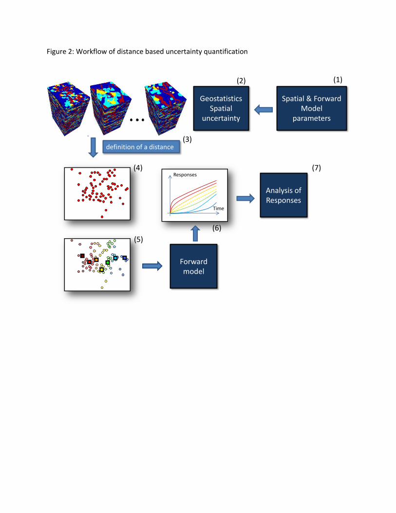
Figure 2: Workflow of distance based uncertainty quantification

definition of a distance

(1)

(3)

(4)

(5)

Responses

Time

Spatial & ForwardModel

parameters

GeostatisticsSpatial

uncertainty

(2)

Forwardmodel

(6)

Analysis ofResponses

(7)

Figure 3: Application of k-medoid and kernel k-medoid clustering to generate cluster models

Figure 4: Overview of software structure of SGEMS-UQ and data flow of SGEMS-UQ program

Figure 5: Data mining base classes structure. Future modules can be easily added by inheriting

from the two base classes.

Figure 6: Selection of two 3D training images with each having two sample facies models

generated using SGEMS program snesim.

Training image Facies models from SGEMS

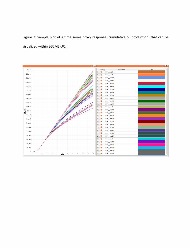
Figure 7: Sample plot of a time series proxy response (cumulative oil production) that can be

visualized within SGEMS-UQ.

Figure 8: GUI interface used to generate MDS space within SGEMS-UQ.

Figure 9: Visualizer for MDS space and parameters in tree format for realization 92. Property

highlighting and other GUI enhancements have been included.

Figure 10: Sample 3D visualization of MDS performed on 100 realizations using Cumulative Oil

Production (over the entire field), as the distance metric. SGEMS-UQ allows for multiple

instances of k-means to be performed.

Figure 11: (a) Cumulative oil production P10, P50 and P90 values and (b) Cumulative water

production response of the 12 realizations selected by KKM compared to P10, P50 and P90

values from exhaustive set.

A B

P90P50

P10

P90

P50

P10

Figure 12: Pareto plot produced by examining sensitivity of facies porosity/permeability means

and variances. The GUI interface for producing Pareto plots is also shown.

Figure 13: Data mining of parameter value within a cluster. This operation plots the mean value

of the histogram used to generate the permeability map for facies 2 of all properties within a

particular cluster.

Figure 14: Data mining interface over all the realizations. This particular instance returns and

plots all realizations with facies3 permeability standard deviation less than that of realization

NTG_real28. This can also be used to return realizations with a parameter within a certain

range of a baseline realization.

Figure 15: Data mining interface for locating all realizations with a common parameter value.

Figure 16: Data mining interface for locating all common parameter values given a set of

realizations.

Table 1: Properties of training images

Facies

Architecture

Channel

Thickness

Width/Thickness

Ratio

Channel

Sinuosity

1 0.019 0.025 0.030 25

2 0.113 0.162 0.213 1000

3 0.151 0.191 0.231 1430

Table 2: Mean values of target histograms used to generate porosity and permeability

Facies

Architecture

Channel

Thickness

Width/Thickness

Ratio

Channel

Sinuosity

1 0.019 0.025 0.030 25

2 0.113 0.162 0.213 1000

3 0.151 0.191 0.231 1430

Table 3: Standard deviation of target histograms used to generate porosity and permeability

STD Porosity Permeability

Min Mid Max Min Mid Max

Facies1 0.022 0.027 0.032 25 37 50

Facies2 0.045 0.055 0.065 550 650 750

Facies3 0.048 0.058 0.068 485 585 685

Facies4 0.035 0.045 0.055 295 345 395

Forward model

Geostatistics Spatial

uncertainty

Spatial Model

parameters

Analysis of Responses

Forward model

parameters

Field Data

Figure 1

definition of a distance

(1)

(3)

(4)

(5)

Responses

Time

Spatial & Forward

Model parameters

Geostatistics Spatial

uncertainty

(2)

Forward model

(6)

Analysis of Responses

(7)

Figure 2

Figure 3

Figure 4

Figure 5

Training image Facies models from SGEMS

Figure 6

Figure 7

Figure 8

Figure 9

Figure 10

Figure 11

A B

P90 P50

P10

P90

P50

P10

Figure 12

Figure 13

Figure 14

Figure 15

Figure 16

Facies

Architecture

Channel

Thickness

Width/Thickness

Ratio

Channel

Sinuosity

1 0.019 0.025 0.030 25

2 0.113 0.162 0.213 1000

3 0.151 0.191 0.231 1430

Mean

Porosity Permeability

Min Mid Max Min Mid Max

Facies1 0.019 0.025 0.030 25 50 75

Facies2 0.113 0.162 0.213 1000 1200 1400

Facies3 0.151 0.191 0.231 1430 1630 1830

Facies4 0.190 0.230 0.270 1875 2175 2475

STD Porosity Permeability

Min Mid Max Min Mid Max

Facies1 0.022 0.027 0.032 25 37 50

Facies2 0.045 0.055 0.065 550 650 750

Facies3 0.048 0.058 0.068 485 585 685

Facies4 0.035 0.045 0.055 295 345 395