Embed Size (px)
Citation preview
General rights Copyright and moral rights for the publications made accessible in the public portal are retained by the authors and/or other copyright owners and it is a condition of accessing publications that users recognise and abide by the legal requirements associated with these rights.
Users may download and print one copy of any publication from the public portal for the purpose of private study or research.
You may not further distribute the material or use it for any profit-making activity or commercial gain
You may freely distribute the URL identifying the publication in the public portal If you believe that this document breaches copyright please contact us providing details, and we will remove access to the work immediately and investigate your claim.
Downloaded from orbit.dtu.dk on: Feb 21, 2022
Shear and Turbulence Effects on Lidar Measurements
Courtney, Michael; Sathe, Ameya; Gayle Nygaard, Nicolai
Publication date:2014
Document VersionPublisher's PDF, also known as Version of record
Link back to DTU Orbit
Citation (APA):Courtney, M., Sathe, A., & Gayle Nygaard, N. (2014). Shear and Turbulence Effects on Lidar Measurements.DTU Wind Energy. DTU Wind Energy E No. 0061
De
pa
rtm
en
t o
f
Win
d E
ne
rgy
I-R
ep
ort
Shear and Turbulence Effects on Lidar Measurements
Michael Courtney(1)
, Ameya Sathe(1)
and Nicolai Gayle
Nygaard(2)
(1) DTU Wind Energy, (2) DONG Energy
DTU Wind Energy E-0061
October 2014
Author (s): Michael Courtney1 Ameya Sathe
1 and Nicolai
Gayle Nygaard2
Title: on Lidar Measurements
Department: Department of Wind Energy (1)
Collaborating with: DONG Energy (2)
DTU Wind Energy E-0061
October 2014
Summary (max 2000 characters):
Wind lidars are now used extensively for wind resource
measurements. It is known that lidar wind speed measure-
ments are affected by both turbulence and wind shear. This
report explains the mechanisms behind these sensitivities.
For turbulence, it is found that errors in the scalar mean
speed are usually only small. However, particularly in re-
spect of a lidar calibration procedure, turbulence induced
errors in the cup anemometer speed are seen to be signifi-
cantly larger.
Wind shear is shown to induce measurement errors both
due to possible imperfections in the lidar sensing height
and due to the averaging of a non-linear speed profile. Both
effects in combination have to be included when modelling
the lidar error. Attempts to evaluate the lidar error from ex-
perimental data have not been successful probably due to a
lack of detailed knowledge of both the wind shear and the
actual lidar sensing weighting functions.
Contract no.:
[Tekst]
Project no.:
[Tekst]
Sponsor:
DONG Energy
Frontpage:
[Tekst]
Pages: 29
Tables: 0
References: 6
ISBN nr.: 978-87-93278-01-1
Technical University of Denmark
Department of Wind Energy
Frederiksborgvej 399
Building 118
4000 Roskilde
Denmark
Telefon +45 2132 7248
www.vindenergi.dtu.dk

Preface
This is the second of two reports in the DONG Energy funded research project ‘Bankable lidar’
and deals primarily with the effect of shear and turbulence on the calibration results of lidars.
The first report studied the long term stability of calibration results for Leosphere Windcube li-
dars but also concluded that the repeatability of lidar calibrations is rather poor, most probably
due to the varying effects of turbulence and shear. This report attempts to shed some light on
shear and turbulence effects on the calibration.
This is a revised version of the original report, incorporating comments from the reviewers.
DTU Wind Energy
Content
1. Introduction ................................................................................................................ 6
2. Turbulence effects ...................................................................................................... 6 2.1 How turbulence can influence a lidar measurement ...................................................... 6
2.2 Comparing vector and scalar averaging ....................................................................... 7 2.3 Some results from modelling ......................................................................................12
2.4 Examining how turbulence affects a cup anemometer ..................................................14
2.5 Cup turbulence corrected calibration results ................................................................16
3. Shear effects.............................................................................................................18
3.1 Introduction ...............................................................................................................18 3.2 Geometry of lidar wind speed measurements ..............................................................18
3.3 Effect of shear on the lidar wind speed measurement ..................................................21
3.4 Lidar shear error for a power law profile ......................................................................22 3.5 Lidar shear error using measured wind speed profiles ..................................................24
3.6 Calibration results corrected for cup turbulence and lidar shear effects .........................24
4. Discussion ................................................................................................................26 4.1 Turbulence effects .....................................................................................................26
4.2 Shear effects.............................................................................................................27
5. Conclusion ................................................................................................................27
References .........................................................................................................................28
DTU Wind Energy The long term stability of lidar calibrations 5
Summary
Wind lidars are now used extensively for wind resource measurements. It is known that lidar
wind speed measurements are affected by both turbulence and wind shear. This report explains
the mechanisms behind these sensitivities. For turbulence, it is found that errors in the scalar
mean speed are usually only small. However, particularly in respect of a lidar calibration proce-
dure, turbulence induced errors in the cup anemometer speed are seen to be significantly larg-
er.
Wind shear is shown to induce measurement errors both due to possible imperfections in the
lidar sensing height and due to the averaging of a non-linear speed profile. Both effects in com-
bination have to be included when modelling the lidar error. Attempts to evaluate the lidar error
from experimental data have not been successful probably due to a lack of detailed knowledge
of both the wind shear and the actual lidar sensing weighting functions.
DTU Wind Energy The long term stability of lidar calibrations 6
1. Introduction
This is the second of two reports in the DONG Energy funded research project ‘Bankable lidar’
which has the overall aim of documenting the bankability of wind lidars The first report studied
the long term stability of calibration results for Leosphere Windcube lidars. No significant long
term bias (drift) could be identified but it was also concluded that the repeatability of lidar cal i-
brations is rather poor, most probably due to the varying effects of turbulence and shear.
This report attempts to shed some light on shear and turbulence effects on the calibration. We
will briefly outline the mechanisms through which turbulence and shear can affect a lidar meas-
urement. In the case of turbulence, studied in Section 2, this is through errors in the scalar
mean induced by over-sensitivity to lateral turbulence components. Shear induced differences
between lidar and cup wind speeds, treated in Section 3, arise since the lidar, rather than
measuring at a point, measures a weighted average of speeds over a significant height range.
Throughout the report we will use the term lidar error to describe the deviation between the 10-
minute mean lidar wind speed and the corresponding wind speed of the reference at a given
height.
The report rounds off with a discussion (Section 4) including recommendations on how to im-
prove lidar accuracy both with respect to turbulence and shear and conclusions in Section 5.
2. Turbulence effects
2.1 How turbulence can influence a lidar measurement
Turbulence is one of the most obvious parameters that both varies widely during the course of a
lidar calibration and can be expected to have an influence on the lidar’s measurements. Since
turbulence and shear are closely linked through the stratification (stability), identifying a clear re-
lationship between lidar measurement ‘errors’ (discrepancies between the lidar and reference
cup speeds) is not possible.
Several observations of apparent lidar over-speeding in summer periods with prevailing unsta-
ble stability have led to a closer examination of the possible cause. Current lidar calibration pro-
cedures and most lidar applications perform a 10 minute scalar average of the wind speed. On
the Windcube this means that an averaging is performed on the reconstructed horizontal wind
speeds that are calculated after each new line-of-sight measurement is completed, a rate of
about 1 Hz. Cup anemometer data are inherently a scalar value (there is no information regard-
ing the direction of the wind) and an average cup anemometer wind speed is almost invariably a
scalar mean.
Scalar averaging is an averaging of the instantaneous wind speed (or the length of the instanta-
neous wind speed vector). It will always be larger than the vector mean speed which is the
length of the vector formed by the averaged orthogonal wind speed components. An extreme
DTU Wind Energy The long term stability of lidar calibrations 7
case that demonstrates this well is if the wind speed blows at speed U in one direction for 5
minutes and then blows, still at speed U, in the 180° reverse direction for the next 5 minutes. A
scalar mean will not ‘see’ the change in wind speed – the mean will be U. The vector mean
speed will however be zero.
More formally, the difference between the vector mean 𝑈 and the scalar mean 𝑈𝑠 can fairly
easily be shown ([6]) to be
𝑈𝑠 = 𝑈(1 + 𝜎𝑣
2
2𝑈2)
where 𝜎𝑣 is the transverse turbulence component. Clearly, the difference between the vector
and scalar mean will depend on the magnitude of the transverse turbulence. The scalar average
wind speeds from two different sensors, co-located and measuring simultaneously but having
different sensitivities to the transverse turbulence component, will therefore also be different. It
is this mechanism that we suspected as the explanation for the lidar-cup speed discrepancies in
high turbulence. In the following section, a period of lidar calibration data is analysed to illumi-
nate differences between scalar and vector averaging.
2.2 Comparing vector and scalar averaging
In order to investigate the differences between scalar and vector averaging methods, we have
studied a two month period of Windcube and reference mast data from the Høvsøre test site.
The data is for Windcube WLS7-139 whilst it was standing beside the Høvsøre 116m met mast
between 1 April and 5th
June 2013. This met mast and lidar position are well known as they form
the basis of the DTU accredited lidar calibration. In this study, we only consider the data meas-
ured at a height of 80m.
To be consistent with our normal calibration procedure, we have filtered the data according to
the following criteria:
Wind direction between 230 and 300
Wind speed between 4 and 16 m/s
Temperature greater than 2°C
Lidar availability in a given 10 minute period > 90%
The availability criterion is slightly relaxed in relation to our standard calibration procedure
where an availability of 100% is required. Applying these criteria results in a dataset of 1248
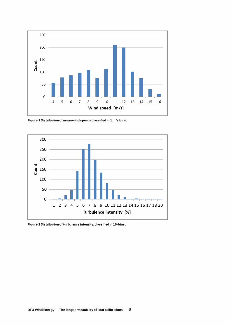
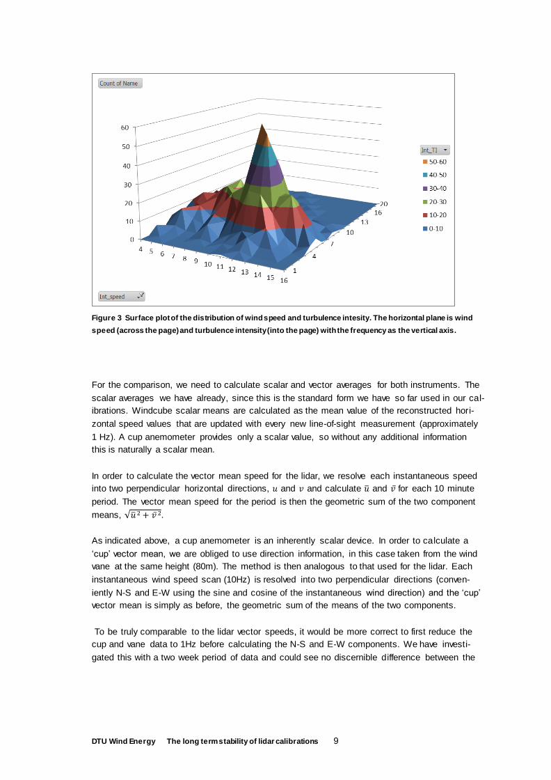
points. Distributions of speed and turbulence intensity are shown in Figure 1 and Figure 2 re-
spectively. A surface plot of the distribution as a function of both speed and turbulence intensity
is shown in Figure 3.
DTU Wind Energy The long term stability of lidar calibrations 8
Figure 1 Distribution of mean wind speeds classified in 1 m/s bins.
Figure 2 Distribution of turbulence intensity, classified in 1% bins.
DTU Wind Energy The long term stability of lidar calibrations 9
Figure 3 Surface plot of the distribution of wind speed and turbulence intesity. The horizontal plane is wind
speed (across the page) and turbulence intensity (into the page) with the frequency as the vertical axis.
For the comparison, we need to calculate scalar and vector averages for both instruments. The
scalar averages we have already, since this is the standard form we have so far used in our cal-
ibrations. Windcube scalar means are calculated as the mean value of the reconstructed hori-
zontal speed values that are updated with every new line-of-sight measurement (approximately
1 Hz). A cup anemometer provides only a scalar value, so without any additional information
this is naturally a scalar mean.
In order to calculate the vector mean speed for the lidar, we resolve each instantaneous speed
into two perpendicular horizontal directions, 𝑢 and 𝑣 and calculate �̅� and �̅� for each 10 minute
period. The vector mean speed for the period is then the geometric sum of the two component
means, √�̅� 2 + �̅� 2.
As indicated above, a cup anemometer is an inherently scalar device. In order to calculate a
‘cup’ vector mean, we are obliged to use direction information, in this case taken from the wind
vane at the same height (80m). The method is then analogous to that used for the lidar. Each
instantaneous wind speed scan (10Hz) is resolved into two perpendicular directions (conven-
iently N-S and E-W using the sine and cosine of the instantaneous wind direction) and the ‘cup’
vector mean is simply as before, the geometric sum of the means of the two components.
To be truly comparable to the lidar vector speeds, it would be more correct to first reduce the
cup and vane data to 1Hz before calculating the N-S and E-W components. We have investi-
gated this with a two week period of data and could see no discernible difference between the
DTU Wind Energy The long term stability of lidar calibrations 10
vector wind speeds calculated using the two different methods. We therefor believe the compar-
isons made between the lidar and (10Hz) cup vector speeds to be fully justified.
A sonic anemometer is also available at 80m, although on the N side of the mast whereas the
cup and vanes are installed on the S side. Nevertheless, we will also use the vector mean
speed from the sonic anemometer (derived from the geometric sum of the mean x and y com-
ponents) in the following analysis.
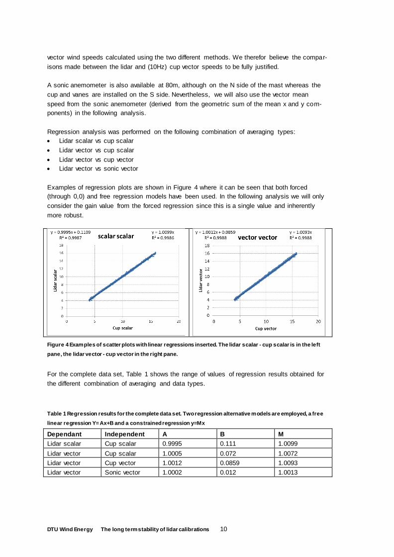
Regression analysis was performed on the following combination of averaging types:
Lidar scalar vs cup scalar
Lidar vector vs cup scalar
Lidar vector vs cup vector
Lidar vector vs sonic vector
Examples of regression plots are shown in Figure 4 where it can be seen that both forced
(through 0,0) and free regression models have been used. In the following analysis we will only
consider the gain value from the forced regression since this is a single value and inherently
more robust.
Figure 4 Examples of scatter plots with linear regressions inserted. The lidar scalar - cup scalar is in the left
pane, the lidar vector - cup vector in the right pane.
For the complete data set, Table 1 shows the range of values of regression results obtained for
the different combination of averaging and data types.
Table 1 Regression results for the complete data set. Two regression alternative models are employed, a free
linear regression Y= Ax+B and a constrained regression y=Mx
Dependant Independent A B M
Lidar scalar Cup scalar 0.9995 0.111 1.0099
Lidar vector Cup scalar 1.0005 0.072 1.0072
Lidar vector Cup vector 1.0012 0.0859 1.0093
Lidar vector Sonic vector 1.0002 0.012 1.0013
DTU Wind Energy The long term stability of lidar calibrations 11
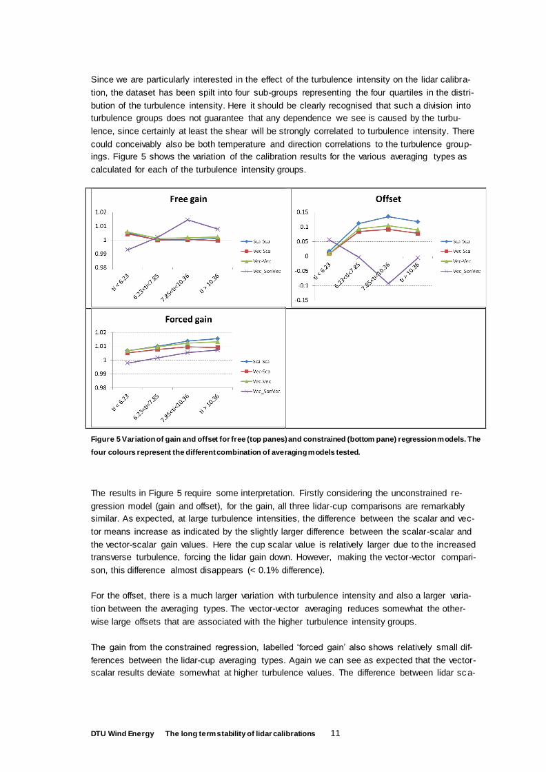
Since we are particularly interested in the effect of the turbulence intensity on the lidar calibra-
tion, the dataset has been spilt into four sub-groups representing the four quartiles in the distri-
bution of the turbulence intensity. Here it should be clearly recognised that such a division into
turbulence groups does not guarantee that any dependence we see is caused by the turbu-
lence, since certainly at least the shear will be strongly correlated to turbulence intensity. There
could conceivably also be both temperature and direction correlations to the turbulence group-
ings. Figure 5 shows the variation of the calibration results for the various averaging types as
calculated for each of the turbulence intensity groups.
Figure 5 Variation of gain and offset for free (top panes) and constrained (bottom pane) regression models. The
four colours represent the different combination of averaging models tested.
The results in Figure 5 require some interpretation. Firstly considering the unconstrained re-
gression model (gain and offset), for the gain, all three lidar-cup comparisons are remarkably
similar. As expected, at large turbulence intensities, the difference between the scalar and vec-
tor means increase as indicated by the slightly larger difference between the scalar-scalar and
the vector-scalar gain values. Here the cup scalar value is relatively larger due to the increased
transverse turbulence, forcing the lidar gain down. However, making the vector-vector compari-
son, this difference almost disappears (< 0.1% difference).
For the offset, there is a much larger variation with turbulence intensity and also a larger varia-
tion between the averaging types. The vector-vector averaging reduces somewhat the other-
wise large offsets that are associated with the higher turbulence intensity groups.
The gain from the constrained regression, labelled ‘forced gain’ also shows relatively small dif-
ferences between the lidar-cup averaging types. Again we can see as expected that the vector-
scalar results deviate somewhat at higher turbulence values. The difference between lidar sc a-
DTU Wind Energy The long term stability of lidar calibrations 12
lar-scalar and lidar vector-vector forced gains is very small at low turbulence intensities, the dif-
ference growing somewhat with turbulence intensity but is no more than 0.25% for the highest
turbulence intensity group.
Overall, the most striking aspect of the forced gain is that for all averaging types , there is a clear
increase with turbulence intensity. The difference for the vector-vector averaging is around 0.7%
over the range of turbulence intensities in this dataset. Whilst this trend may not necessarily be
directly related to turbulence, we have a clear signal here that requires further explanation.
2.3 Some results from modelling
As explained in section Error! Reference source not found., scalar means are sensitive to the
ransverse turbulence component that the instrument senses. Over-sensitivity to the transverse
component, for example as seen in a 2-beam nacelle lidar, will result in an over-speeding of the
scalar mean speed. In such as case, the reported scalar mean will be higher than true scalar
mean which in turn will always be higher than the vector mean speed. A cup anemometer, that
is unable to sense transverse components, will always report the correct scalar speed (assum-
ing everything else is perfect). In both cases however, the difference between the scalar and
vector mean will increase as the transverse turbulence increases.
A good model for predicting how a Windcube lidar senses turbulence exists [3]. Basically this
model uses the Mann model to represent the 3D structure and statistics of the turbulence and
calculates how a lidar operating in such a 3D field will sense the turbulence fluctuations in com-
parison to the true turbulence. Often an ideal sonic anemometer is used to represent ‘true’ tur-
bulence.
We have used this model to calculate how well the transverse turbulence is sensed by a
Windcube in comparison with a sonic anemometer. The example shown in Figure 6 is for neu-
tral conditions and a height of 80m. Parameters for the Mann model are derived from spectra
previously measured at the Høvsøre met mast. What is shown in the plot is the modelled (full
lines) and measured (open circles) differences between scalar and vector mean speeds for the
Windcube lidar (red) and an ideal sonic (blue). The difference between the blue and the red
lines represents the error that the lidar will make in its scalar mean as a result of its slight over-
sensitivity to the transverse turbulence. For all wind speeds the difference from the modelling is
a few tenths of a percent, consistent with what we have seen above. Also the measured data in
Figure 5 (not the same dataset as used above) show the same order of magnitude of difference.
DTU Wind Energy The long term stability of lidar calibrations 13
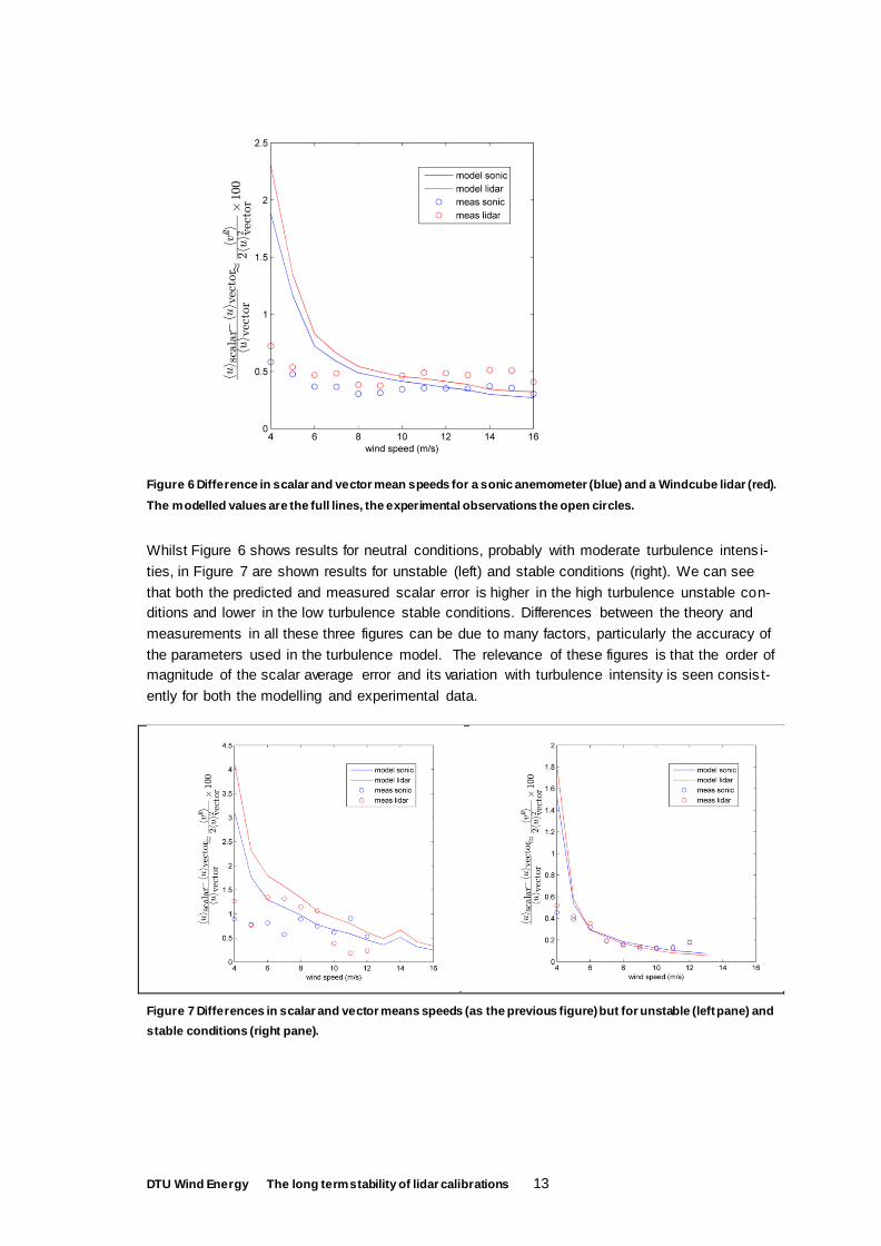
Figure 6 Difference in scalar and vector mean speeds for a sonic anemometer (blue) and a Windcube lidar (red).
The modelled values are the full lines, the experimental observations the open circles.
Whilst Figure 6 shows results for neutral conditions, probably with moderate turbulence intens i-
ties, in Figure 7 are shown results for unstable (left) and stable conditions (right). We can see
that both the predicted and measured scalar error is higher in the high turbulence unstable con-
ditions and lower in the low turbulence stable conditions. Differences between the theory and
measurements in all these three figures can be due to many factors, particularly the accuracy of
the parameters used in the turbulence model. The relevance of these figures is that the order of
magnitude of the scalar average error and its variation with turbulence intensity is seen consis t-
ently for both the modelling and experimental data.
Figure 7 Differences in scalar and vector means speeds (as the previous figure) but for unstable (left pane) and
stable conditions (right pane).
DTU Wind Energy The long term stability of lidar calibrations 14
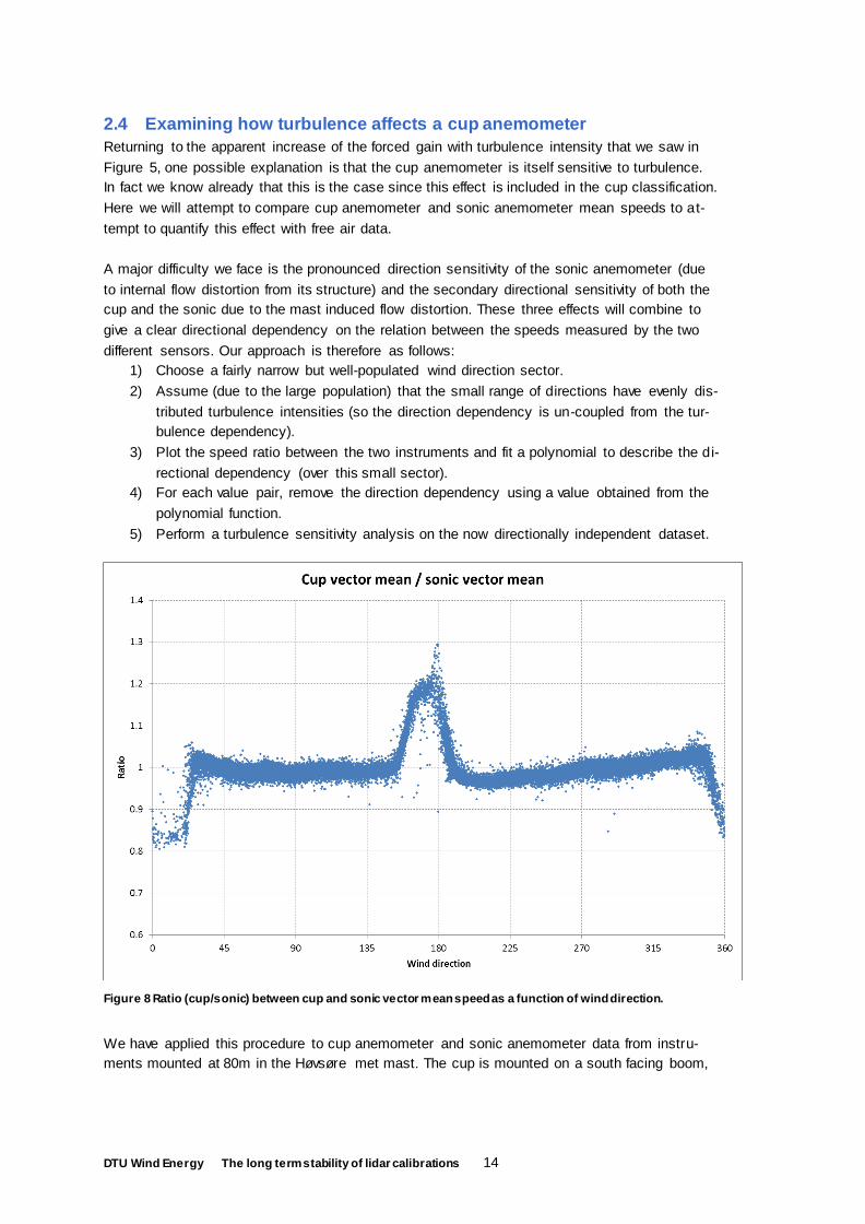
2.4 Examining how turbulence affects a cup anemometer
Returning to the apparent increase of the forced gain with turbulence intensity that we saw in
Figure 5, one possible explanation is that the cup anemometer is itself sensitive to turbulence.
In fact we know already that this is the case since this effect is included in the cup classification.
Here we will attempt to compare cup anemometer and sonic anemometer mean speeds to at-
tempt to quantify this effect with free air data.
A major difficulty we face is the pronounced direction sensitivity of the sonic anemometer (due
to internal flow distortion from its structure) and the secondary directional sensitivity of both the
cup and the sonic due to the mast induced flow distortion. These three effects will combine to
give a clear directional dependency on the relation between the speeds measured by the two
different sensors. Our approach is therefore as follows:
1) Choose a fairly narrow but well-populated wind direction sector.
2) Assume (due to the large population) that the small range of directions have evenly dis-
tributed turbulence intensities (so the direction dependency is un-coupled from the tur-
bulence dependency).
3) Plot the speed ratio between the two instruments and fit a polynomial to describe the di-
rectional dependency (over this small sector).
4) For each value pair, remove the direction dependency using a value obtained from the
polynomial function.
5) Perform a turbulence sensitivity analysis on the now directionally independent dataset.
Figure 8 Ratio (cup/sonic) between cup and sonic vector mean speed as a function of wind direction.
We have applied this procedure to cup anemometer and sonic anemometer data from instru-
ments mounted at 80m in the Høvsøre met mast. The cup is mounted on a south facing boom,
DTU Wind Energy The long term stability of lidar calibrations 15
the sonic on a north facing boom. For all wind directions, the ratio between the cup and the son-
ic is as shown in Figure 8. For both instruments, we have used a vector averaging, for the cup
anemometer using the adjacent wind vane to first resolve into N-S and E-W components. For
the sonic anemometer the initial resolution of the data is 20Hz, for the cup anemometer it is
10Hz. As expected, both because of the mast distortion and the internal flow distortion of the
sonic anemometer, there is a pronounced variation as a function of wind direction.
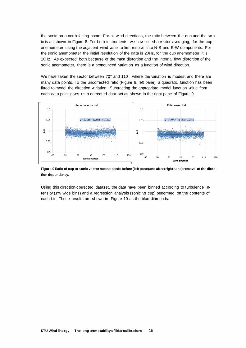
We have taken the sector between 70° and 110°, where the variation is modest and there are
many data points. To the uncorrected ratio (Figure 9, left pane), a quadratic function has been
fitted to model the direction variation. Subtracting the appropriate model function value from
each data point gives us a corrected data set as shown in the right pane of Figure 9.
Figure 9 Ratio of cup to sonic vector mean speeds before (left pane) and after (right pane) removal of the direc-
tion dependency.
Using this direction-corrected dataset, the data have been binned according to turbulence in-
tensity (1% wide bins) and a regression analysis (sonic vs cup) performed on the contents of
each bin. These results are shown in Figure 10 as the blue diamonds.
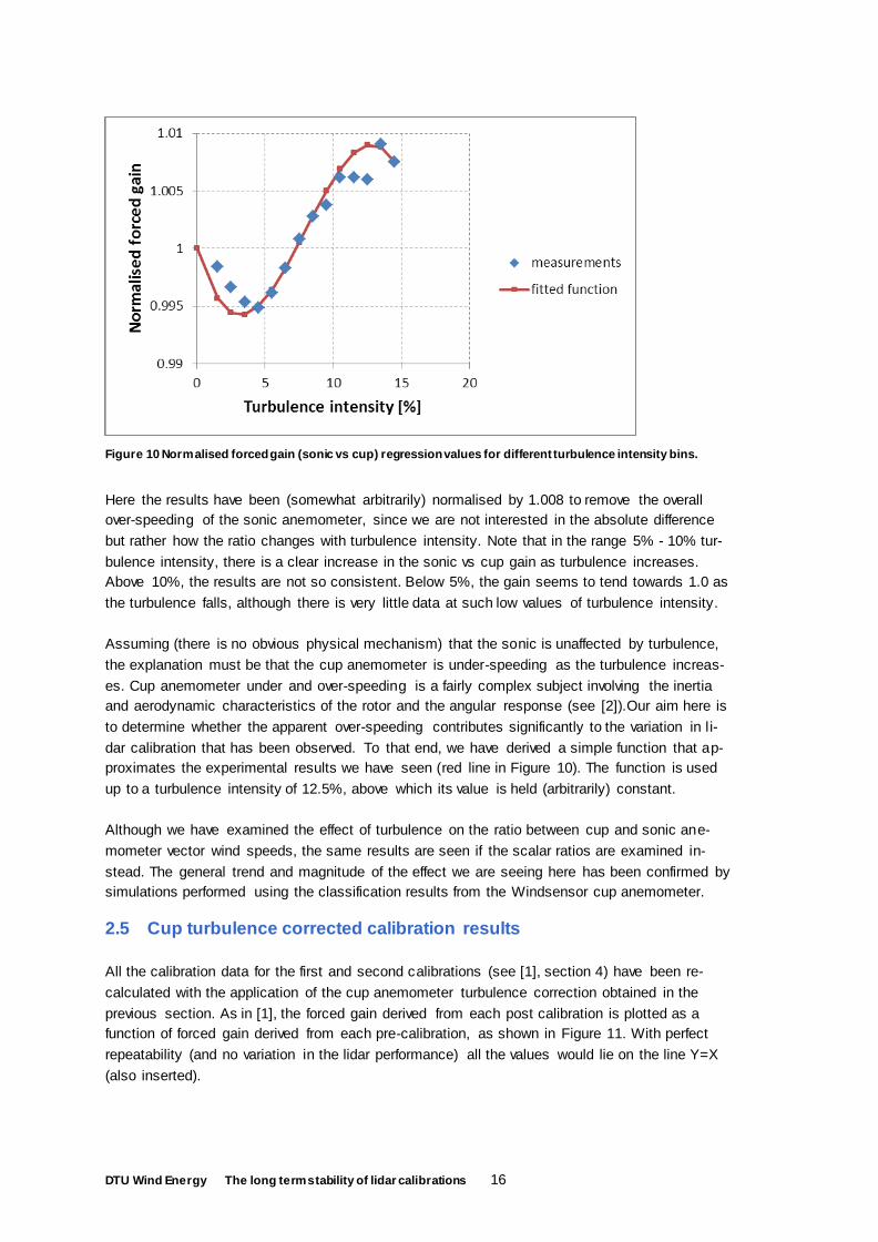
DTU Wind Energy The long term stability of lidar calibrations 16
Figure 10 Normalised forced gain (sonic vs cup) regression values for different turbulence intensity bins.
Here the results have been (somewhat arbitrarily) normalised by 1.008 to remove the overall
over-speeding of the sonic anemometer, since we are not interested in the absolute difference
but rather how the ratio changes with turbulence intensity. Note that in the range 5% - 10% tur-
bulence intensity, there is a clear increase in the sonic vs cup gain as turbulence increases.
Above 10%, the results are not so consistent. Below 5%, the gain seems to tend towards 1.0 as
the turbulence falls, although there is very little data at such low values of turbulence intensity.
Assuming (there is no obvious physical mechanism) that the sonic is unaffected by turbulence,
the explanation must be that the cup anemometer is under-speeding as the turbulence increas-
es. Cup anemometer under and over-speeding is a fairly complex subject involving the inertia
and aerodynamic characteristics of the rotor and the angular response (see [2]).Our aim here is
to determine whether the apparent over-speeding contributes significantly to the variation in li-
dar calibration that has been observed. To that end, we have derived a simple function that ap-
proximates the experimental results we have seen (red line in Figure 10). The function is used
up to a turbulence intensity of 12.5%, above which its value is held (arbitrarily) constant.
Although we have examined the effect of turbulence on the ratio between cup and sonic ane-
mometer vector wind speeds, the same results are seen if the scalar ratios are examined in-
stead. The general trend and magnitude of the effect we are seeing here has been confirmed by
simulations performed using the classification results from the Windsensor cup anemometer.
2.5 Cup turbulence corrected calibration results
All the calibration data for the first and second calibrations (see [1], section 4) have been re-
calculated with the application of the cup anemometer turbulence correction obtained in the
previous section. As in [1], the forced gain derived from each post calibration is plotted as a
function of forced gain derived from each pre-calibration, as shown in Figure 11. With perfect
repeatability (and no variation in the lidar performance) all the values would lie on the line Y=X
(also inserted).
DTU Wind Energy The long term stability of lidar calibrations 17
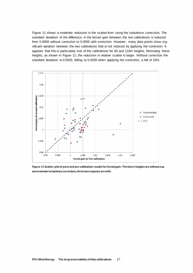
Figure 11 shows a moderate reduction in the scatter from using the turbulence correction. The
standard deviation of the difference in the forced gain between the two calibrations is reduced
from 0.0059 without correction to 0.0055 with correction. However, many data points show sig-
nificant variation between the two calibrations that is not reduced by applying the correction. It
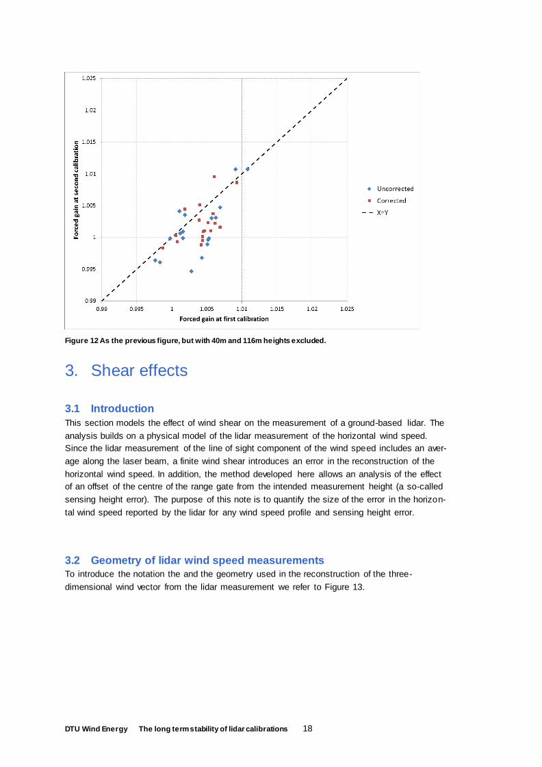
appears that this is particularly true of the calibrations for 40 and 116m heights. Removing these
heights, as shown in Figure 12, the reduction in relative scatter is larger. Without correction the
standard deviation is 0.0033, falling to 0.0028 when applying the correction, a fall of 15%.
Figure 11 Scatter plot of post and pre-calibration results for forced gain. The blue triangles are without cup
anemometer turbulence correction, the brown squares are with.
DTU Wind Energy The long term stability of lidar calibrations 18
Figure 12 As the previous figure, but with 40m and 116m heights excluded.
3. Shear effects
3.1 Introduction
This section models the effect of wind shear on the measurement of a ground-based lidar. The
analysis builds on a physical model of the lidar measurement of the horizontal wind speed.
Since the lidar measurement of the line of sight component of the wind speed includes an aver-
age along the laser beam, a finite wind shear introduces an error in the reconstruction of the
horizontal wind speed. In addition, the method developed here allows an analysis of the effect
of an offset of the centre of the range gate from the intended measurement height (a so-called
sensing height error). The purpose of this note is to quantify the size of the error in the horizon-
tal wind speed reported by the lidar for any wind speed profile and sensing height error.
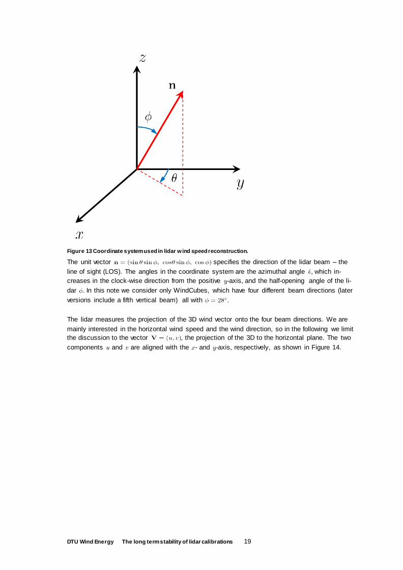
3.2 Geometry of lidar wind speed measurements
To introduce the notation the and the geometry used in the reconstruction of the three-
dimensional wind vector from the lidar measurement we refer to Figure 13.
DTU Wind Energy The long term stability of lidar calibrations 19
Figure 13 Coordinate system used in lidar w ind speed reconstruction.
The unit vector specifies the direction of the lidar beam – the
line of sight (LOS). The angles in the coordinate system are the azimuthal angle , which in-
creases in the clock-wise direction from the positive -axis, and the half-opening angle of the li-
dar . In this note we consider only WindCubes, which have four different beam directions (later
versions include a fifth vertical beam) all with .
The lidar measures the projection of the 3D wind vector onto the four beam directions. We are
mainly interested in the horizontal wind speed and the wind direction, so in the following we limit
the discussion to the vector , the projection of the 3D to the horizontal plane. The two
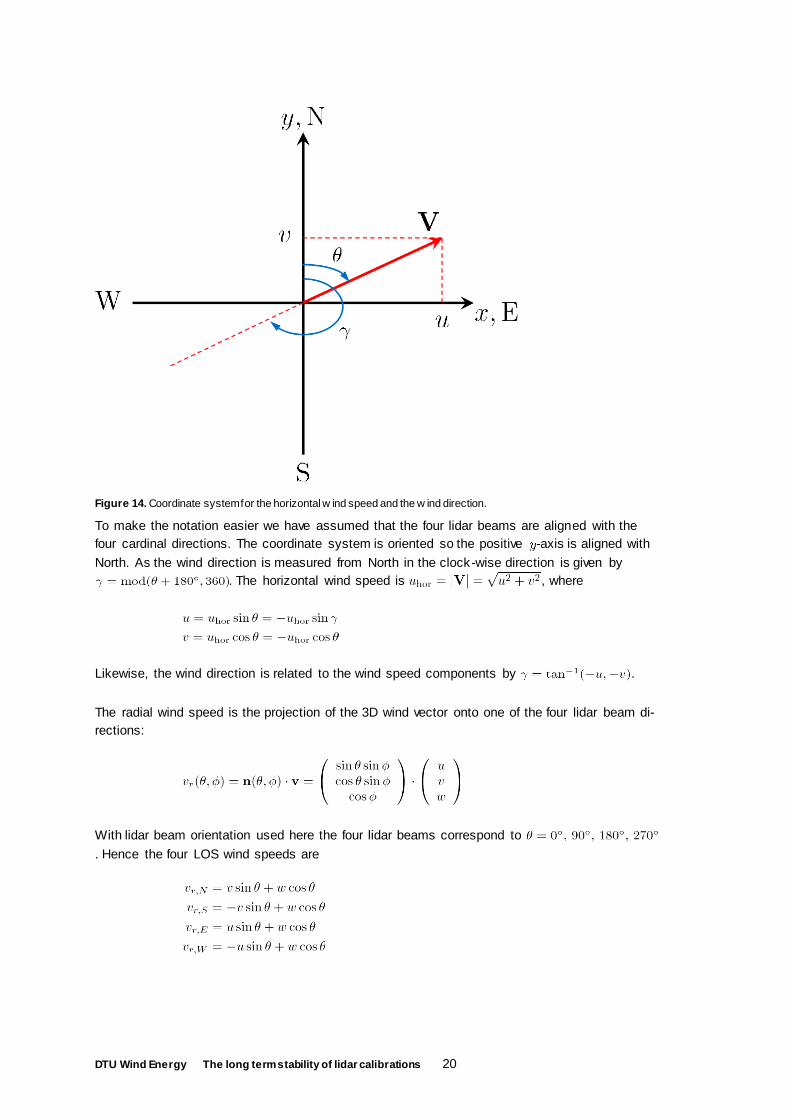
components and are aligned with the - and -axis, respectively, as shown in Figure 14.
DTU Wind Energy The long term stability of lidar calibrations 20
Figure 14. Coordinate system for the horizontal w ind speed and the w ind direction.
To make the notation easier we have assumed that the four lidar beams are aligned with the
four cardinal directions. The coordinate system is oriented so the positive -axis is aligned with
North. As the wind direction is measured from North in the clock-wise direction is given by
. The horizontal wind speed is , where
Likewise, the wind direction is related to the wind speed components by .
The radial wind speed is the projection of the 3D wind vector onto one of the four lidar beam di-
rections:
With lidar beam orientation used here the four lidar beams correspond to
. Hence the four LOS wind speeds are
DTU Wind Energy The long term stability of lidar calibrations 21
Based on these relations the components of the horizontal wind speed can be reconstructed as
(1)
(2)
These expressions involve the radial wind speed found by projecting the true 3D wind vector on
the lidar LOS. In the next section we consider the modification required to describe what the l i-
dar actually measures.
3.3 Effect of shear on the lidar wind speed measurement
The lidar does not measure the LOS wind speed at a single point. Rather the LOS wind speed
is averaged along the beam due to the finite pulse length defining the range gate. We use the
following model of the lidar LOS wind speed measurement:
(3)
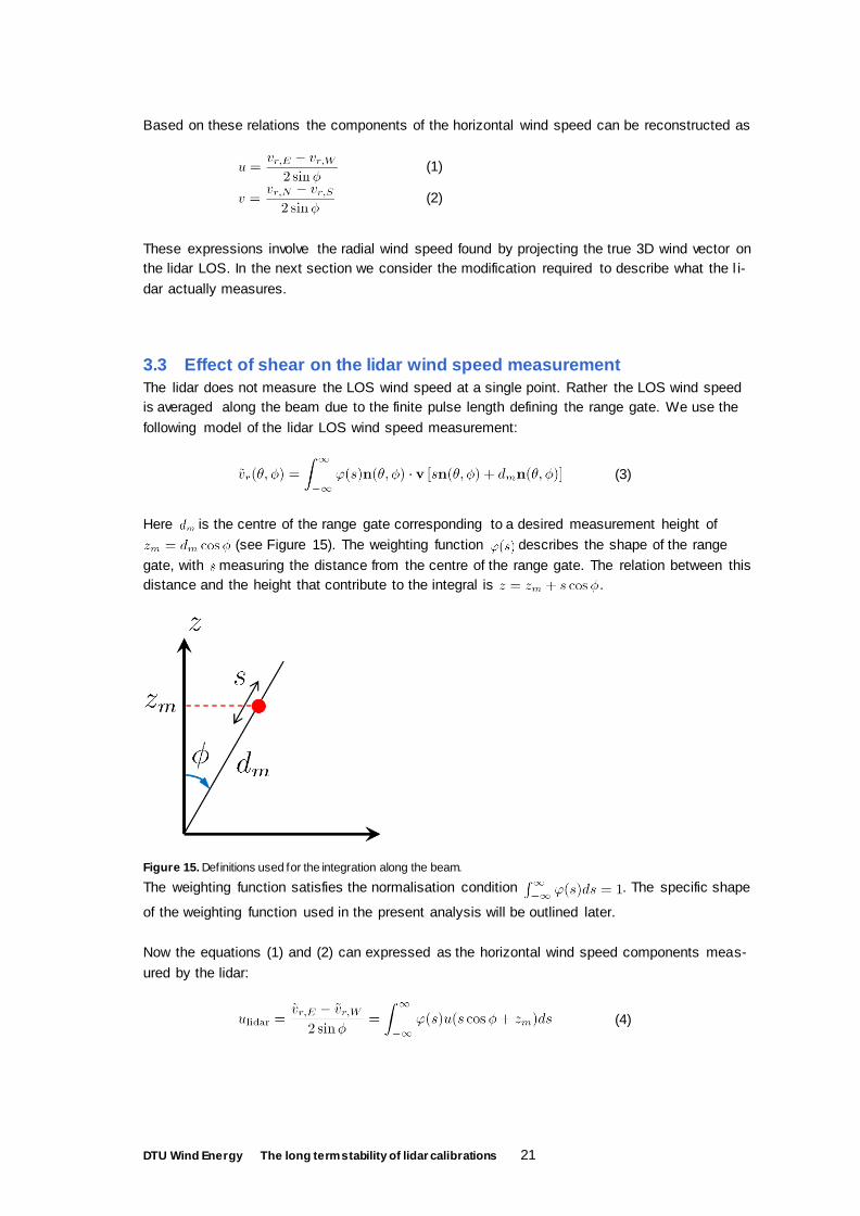
Here is the centre of the range gate corresponding to a desired measurement height of
(see Figure 15). The weighting function describes the shape of the range
gate, with measuring the distance from the centre of the range gate. The relation between this
distance and the height that contribute to the integral is .
Figure 15. Definitions used for the integration along the beam.
The weighting function satisfies the normalisation condition . The specific shape
of the weighting function used in the present analysis will be outlined later.
Now the equations (1) and (2) can expressed as the horizontal wind speed components meas-
ured by the lidar:
(4)
DTU Wind Energy The long term stability of lidar calibrations 22
(5)
In the presence of shear and veer the horizontal wind speed and the wind direction depend on
height, hence
(6)
(7)
The model for the horizontal wind speed measured by the lidar is then
(8)
using equations (4), (5), (6), and (7). This takes the shear profile into account through the varia-
tion of the true wind speed components with height.
At the present stage we neglect any veer by setting and equating this with the wind di-
rection at the measurement height. In that case the wind direction dependent factors and
for and , respectively, can be taken outside the integral and the expression simpl i-
fies considerably:
(no wind veer)
3.4 Lidar shear error for a power law profile
For a power law wind speed profile we can quantify the lidar wind speed error as a function of
the shear. We assume the wind speed profile
Here and is the wind shear parameter. In addition, we include a sensing
height error , which is the offset between the desired and the actual measurement height:
. Note that the lidar error due to shear is a deviation of the lidar wind speed from
what a reference cup anemometer would measure at the same height, whereas the sensing
height error is a measure of the imperfect c of the lidar range gate.
(9)
Finally, we use for the weighting function
(10)
DTU Wind Energy The long term stability of lidar calibrations 23
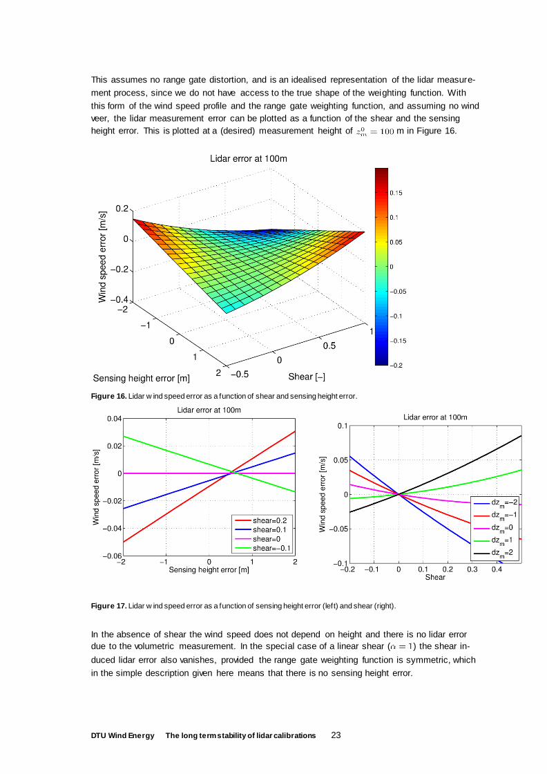
This assumes no range gate distortion, and is an idealised representation of the lidar measure-
ment process, since we do not have access to the true shape of the weighting function. With
this form of the wind speed profile and the range gate weighting function, and assuming no wind
veer, the lidar measurement error can be plotted as a function of the shear and the sensing
height error. This is plotted at a (desired) measurement height of m in Figure 16.
Figure 16. Lidar w ind speed error as a function of shear and sensing height error.
Figure 17. Lidar w ind speed error as a function of sensing height error (left) and shear (right).
In the absence of shear the wind speed does not depend on height and there is no lidar error
due to the volumetric measurement. In the special case of a linear shear ( ) the shear in-
duced lidar error also vanishes, provided the range gate weighting function is symmetric, which
in the simple description given here means that there is no sensing height error.
DTU Wind Energy The long term stability of lidar calibrations 24
We have investigated the effect of veer on the results by adding a linear variation of the wind di-
rection. For a wind direction increasing or decreasing by 0.1°/m there is negligible influence of
veer on the results, so we continue to neglect it. However, in case of a large variation of the
wind direction with height, the veer can easily be incorporated into the analysis by going back to
(8).
3.5 Lidar shear error using measured wind speed profiles To estimate the size of the error incurred from the combination of wind shear and a sensing height error using real wind speed profiles we fit 10-minute wind speed profiles with the expres-
sion
(11)
The fitted profile can then be used in equation (9) to predict the corresponding horizontal wind
speed reported by the lidar, again neglecting veer. As in the previous section we use the trian-
gle-shaped weighting function. The sensing height error is estimated from a 3-parameter fit to
the observed lidar wind speeds at each height.
Based on the model for the lidar horizontal wind speed the error of the lidar measurement under the influence of shear and a sensing height error can be obtained as
(12)
at measurement height . This modelled error can be used to correct the lidar measurement
for the sheared flow:
(13)
If the model could perfectly predict the lidar measurement of the horizontal wind speed, this equation would result in a corrected lidar wind speed equal to the fitted profile at the measure-
ment height. In reality as we will see in the following section, this is not the case, since our model is incomplete and/or inaccurate. For one thing our weighting function for averaging along the beam direction is simplified and does not include the effect of range gate distortion.
3.6 Calibration results corrected for cup turbulence and lidar shear ef-
fects
As in section 2.5, the calibrations have been recalculated, correcting for the effects of turbu-
lence on the cup anemometer (as before) and also including the lidar shear error derived from
the measured sensing height error and the fitted curvature of the shear. The results for all
heights are shown in Figure 18.
It can be clearly seen that the corrected results are worse than the un-corrected, indicating that
as predicted, the model is too inaccurate. As before, the results are also plotted only for the
heights 40, 60 and 80m in Figure 19. The difference between these two figures is striking,
showing that the shear model is mostly failing for the ends of the profile (40 and 116m) where
our knowledge of the curvature and the gradient are little better than guess-work. However,
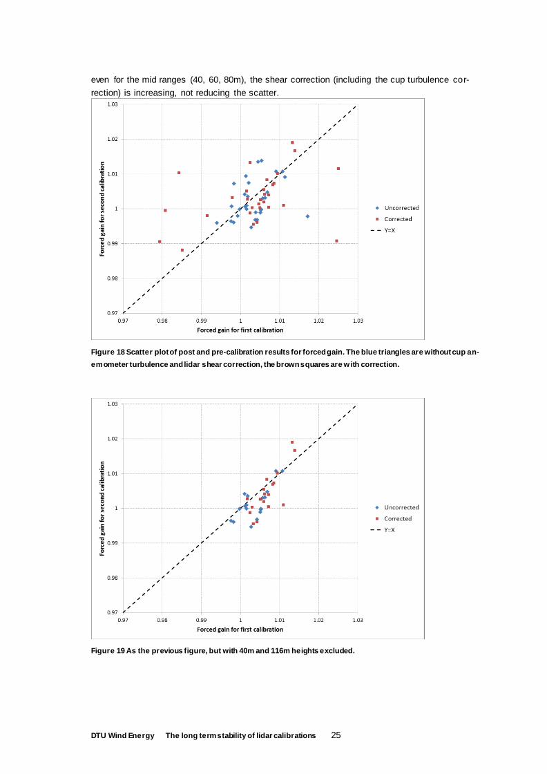
DTU Wind Energy The long term stability of lidar calibrations 25
even for the mid ranges (40, 60, 80m), the shear correction (including the cup turbulence cor-
rection) is increasing, not reducing the scatter.
Figure 18 Scatter plot of post and pre-calibration results for forced gain. The blue triangles are without cup an-
emometer turbulence and lidar shear correction, the brown squares are w ith correction.
Figure 19 As the previous figure, but with 40m and 116m heights excluded.
DTU Wind Energy The long term stability of lidar calibrations 26
4. Discussion
4.1 Turbulence effects
We have seen that the choice of vector or scalar averaging has little effect on the lidar-cup cali-
bration results except at high turbulence intensities. For unstable conditions , the modelling pre-
dicts scalar errors in the order of 0.5% for the lidar (difference between the red and blue lines in
Figure 7, left pane) and these results have been confirmed by experimental observations. For
neutral and stable conditions, the error in the lidar scalar average is typically 0.2% or less. Av-
eraging using vector techniques would give slightly more consistent results especially in unsta-
ble conditions. The differences under normal conditions are probably not large enough to con-
vince the industry of such a dramatic change. Lidar calibrations performed using both tech-
niques could be one possible compromise.
Differences in turbulence intensity seem just as significant however to the cup anemometer per-
formance. We have good evidence of significant cup under-speeding in high turbulence intensi-
ty with a difference of around 1% in speed relative to a sonic anemometer in the range 5 -12%
turbulence intensity. How the cup anemometer performs in this respect at very low turbulence
intensity is almost impossible to measure in free air. This highlights the weakness of calibrating
cup anemometers in very low turbulence wind tunnels. We have no certain method of relating a
cup calibration performed at 0% turbulence intensity with a real-life measurement.
Although the turbulence under/over-speeding of the cup anemometer is recognised in the un-
certainty budget, since the effect is a bias, it would be more appropriate and more consistent
with good uncertainty practice (e.g. GUM [4]) to evaluate and correct for it. To this, we recom-
mend measurement campaigns to be performed in free-air conditions using wind tunnel (Lidar
Doppler Anemometer) calibrated, short range lidars. Using three of these devices mounted in
accurate and stable fixtures it should be possible to measure the true 3D wind vector immedi-
ately in front of a cup anemometer to a reasonably high accuracy. By performing a campaign of
such measurements over a range of environmental conditions (predominantly temperature and
turbulence), the true characteristics of a cup anemometer in at least flat terrain conditions can
be measured.
The value of such measurements would be two-fold. Firstly, the accuracy of cup anemometry
would be improved as reflected by a lower uncertainty. This would have obvious benefits on
cup-based resource assessments and power curve measurements. The second benefit is that
lidars would also be more accurate since their calibration reference uncertainty would be lower
and the calibration repeatability would be higher since the turbulence under/over -speeding of
the cup anemometer would no longer play a role.
An obvious extension of this free-air technique would be to encompass calibration of complete
cup-boom-mast systems so that the cup anemometer mounting uncertainty could be similarly
reduced. Again, through lower calibration reference uncertainty, the benefit to lidars would be a
lower uncertainty and higher calibration repeatability.
DTU Wind Energy The long term stability of lidar calibrations 27
4.2 Shear effects
Whilst we have demonstrated that the effects of both shear curvature and sensing height error
can give significant lidar errors (Figure 16 and Figure 17), the mathematical model developed to
predict and correct for these errors has resulted in increased rather than reduced scatter be-
tween the first and second calibration results (Figure 18). A striking observation is that the scat-
ter is far worse at the ends of the profile (40m and 116m), indicating that our lack of detailed
knowledge of the shear profile is a major factor in our inability to predict the errors. At 40m and
116m where there are no reliable speed measurements below (40m) and above (116m), we
have no good basis for calculating even the first derivative of the speed profile. At all other
heights, although the mean gradient may be acceptable, due to lack of detailed measurements
between the measurement heights (60, 80 and 100m), we are forced to rely on the fitted profile
to provide an estimate of the curvature. Our recommendation here is to increase the vertical
measurement intensity so that a reference speed measurement is available at every 5 or 10m.
Even if we can achieve better resolution of the speed profile, it will not be possible to benefit
from this unless we have better knowledge of the lidar weighting function and how these vary
with height (e.g. due to the effect of the focusing). Our second recommendation with respect to
the shear is to demand thorough documentation from the lidar manufacturers as to how their li-
dars actually sense the wind in the form of weighting functions for the entire range of available
measurement heights.
5. Conclusion
The effects of shear and turbulence on lidar measurements have been investigated, specifically
with respect to the lidar calibration procedure. It has been found through experiments and mod-
elling that Windcube lidar scalar means are only slightly sensitive to turbulence intensity except
in unstable conditions where errors of 0.5% can be experienced. For lidar calibrations, a signifi-
cant under-speeding of the cup anemometer in high turbulence intensity plays a more signifi-
cant role and this should be more thoroughly investigated.
Since the lidar senses over a range of heights, wind shear can also give rise to lidar errors both
due to any significant sensing height error (including possible asymmetry of the weighting func-
tion) and due to the curvature of the profile. Current lidar calibration procedures should be im-
proved to give a higher vertical density of speed measurements including heights beyond (be-
low and above) the calibration height range if possible. In order to model and correct for shear
errors, more detailed information regarding the lidar sensing weighting functions should be re-
quired of the lidar manufacturers.
DTU Wind Energy The long term stability of lidar calibrations 28
References
[1] Michael Courtney and Nicolai Gayle Nygaard, The long term stability of lidar calibrations.
DTU Wind Energy Report E-0033, 2013.
[2] Kristensen L and Hansen O.F., Bias on horizontal mean-wind speed and variance caused
by turbulence. http://www.windsensor.dk/technical/Bias_on_Horizontal_Mean-
Wind_Speed_and_Variance_Caused_by_Turbulence.pdf 2012.
[3] Sathe, A.; Mann, J.; Gottschall, J.; Courtney, M. S. Can Wind Lidars Measure Turbu-
lence? JOURNAL OF ATMOSPHERIC AND OCEANIC TECHNOLOGY,JUL 2011.
[4] Evaluation of measurement data — Guide to the expression of uncertainty in measurement.
(Commonly referred to as GUM). JCGM 100:2008
[5] Gilhousen, D.B., 1987: A field evaluation of NDBC moored buoy winds. Journal of Atmos-
pheric and Oceanic Technology,4, 94-104.
[6] Jakob Mann, Scalar and vector averaging for lidars. Internal DTU Wind Energy note, 2011.

DTU Wind Energy is a department of the Technical University of Denmark with a unique integration of research, education, innovation and
public/private sector consulting in the field of wind energy. Our activities develop new opportunities and technology for the global and Danish
exploitation of wind energy. Research focuses on key technical-scientific fields, which are central for the development, innovation and use of
wind energy and provides the basis for advanced education at the education.
We have more than 230 staff members of which approximately 60 are PhD students. Research is conducted within 9 research programmes or-
ganized into three main topics: Wind energy systems, Wind turbine technology and Basics for wind energy.
Technical University of Denmark
DTU Vindenergi
Frederiksborgvej 399
Building 118
4000 Roskilde
Denmark
Telefon 46 77 50 85
www.vindenergi.dtu.dk