SHEARING AND VOLUMETRIC STRAINING RESPONSE OF …

SHEARING AND VOLUMETRIC STRAINING RESPONSE OF

KIZILIRMAK SAND

A THESIS SUBMITTED TO

THE GRADUATE SCHOOL OF NATURAL AND APPLIED SCIENCES

OF

MIDDLE EAST TECHNICAL UNIVERSITY

BY

ELİFE ÇAKIR

IN PARTIAL FULFILLMENT OF THE REQUIREMENTS

FOR

THE DEGREE OF MASTER OF SCIENCE

IN

CIVIL ENGINEERING

SEPTEMBER 2020

Approval of the thesis:

SHEARING AND VOLUMETRIC STRAINING RESPONSE OF

KIZILIRMAK SAND

submitted by ELİFE ÇAKIR in partial fulfillment of the requirements for the degree

of Master of Science in Civil Engineering, Middle East Technical University by,

Prof. Dr. Halil Kalıpçılar

Dean, Graduate School of Natural and Applied Sciences

Prof. Dr. Ahmet Türer

Head of the Department, Civil Engineering

Prof. Dr. Kemal Önder Çetin

Supervisor, Civil Engineering, METU

Examining Committee Members:

Prof. Dr. Erdal Çokça

Civil Engineering, METU

Prof. Dr. Kemal Önder Çetin


Prof. Dr. Zeynep Gülerce


Prof. Dr. Nihat Sinan Işık

Civil Engineering., Gazi Uni.

Assoc. Prof. Dr. Nabi Kartal Toker


Date: 14.09.2020

iv

I hereby declare that all information in this document has been obtained and

presented in accordance with academic rules and ethical conduct. I also declare

that, as required by these rules and conduct, I have fully cited and referenced

all material and results that are not original to this work.

Name, Last name : Elife Çakır

Signature :

v

ABSTRACT

SHEAR AND VOLUMETRIC STRAINING RESPONSE OF

KIZILIRMAK SAND

Çakır, Elife

Master of Science, Civil Engineering

Supervisor : Prof. Dr. Kemal Önder Çetin

September 2020, 217 pages

The response of sandy soils under monotonic loading depends on size, shape and

mineralogy of particles, fabric, stress, and density states of mixtures. Researchers

around the world have studied their local sands and calibrated their responses (e.g.,

Toyoura sand-Japan, Ottawa sand-Canada, Sacramento sand-US, Sydney sand-

Australia, etc.). However, there are not many studies that have focused on regional

sands from Turkey. This research study aims to introduce a local sand, Kızılırmak

sand, to literature as a "standard sand" from Turkey. For this purpose, shear and

volumetric straining responses of Kızılırmak sand samples were investigated by a

series of consolidated undrained monotonic triaxial and oedometer tests. Specimens

with relative densities of 35-45-60-75 and 80 %, were prepared by wet tamping

method and consolidated under 50 kPa, 100 kPa, 200 kPa and 400 kPa cell pressures,

followed by undrained shearing. Test results were presented by four-way plots,

which enable the individual variations of axial load, cell pressure, pore water

pressure, and axial deformation along with the progress of the stress paths relative to

failure envelopes. On the basis of test results, linear and nonlinear elastic-perfectly

plastic constitutive modeling parameters, including but not limited to stress and

relative-density dependent modulus and effective stress based angles of shearing

vi

resistance, were estimated. Due to its angular nature, Kızılırmak sands' angles of

shearing resistance values of 35.4˚-42.8° were observed, which are closer to the

upper limits of available literature. Triaxial modulus values fall in the range of ~10

and ~160 MPa and are concluded to be in conformance with available literature.

Similarly, samples with varying relative densities, prepared by air pluviation method,

were tested in a conventional oedometer device under stresses starting from ~17 kPa

increasing up to ~33.5 MPa. During tests, unloading and reloading cycles were

performed. Based on these test results, particle crushing-induced yield stresses of

Kızılırmak sands along with their Cc, C values were estimated as ~2.1-4.0 MPa,

~2×10-3-1×10-2, and ~1×10-5–1×10-3, respectively. It was concluded that

Kızılırmak sand exhibited Type B volumetric compression response as defined by

Mesri and Vardhanabhuti (2009). Additionally, test results were also assessed within

critical state framework. Critical state framework soil parameters of angle of steady

state shearing resistances, and values were estimated as 39.4˚, 0.070, and 0.975.

Initial dividing line, defining the boundary between strain hardening and softening

responses, is determined specific for Kızılırmak sand.

Keywords: Triaxial test, One-dimensional volumetric compression, Angle of

shearing resistance, Particle crushing, Kızılırmak sand

vii

ÖZ

KIZILIRMAK KUMUNUN KAYMA VE HACİMSEL BİRİM

DEFORMASYON DAVRANIŞI

Çakır, Elife

Yüksek Lisans, İnşaat Mühendisliği

Tez Yöneticisi: Prof. Dr. Kemal Önder Çetin

Eylül 2020, 217 sayfa

Kumlu zeminlerin statik yükleme altındaki davranışı dane boyutu, şekli,

mineralojisi, dokusu, gerilme ve sıkılık durumları gibi bir çok etken tarafından

kontrol edilmektedir. Araştırmacılar kendi yerel bölgelerinde bulunan kumları

çalışarak kalibre etmiş ve standart kumlar olarak literatüre sunmuşlardır (örneğin;

Toyoura kumu- Japonya, Ottawa kumu- Kanada, Sacramento kumu- ABD, Sydney

kumu- Avusturalya, vb.). Ancak Türkiye'de yerel kumlar üzerinde standart bir kum

geliştirmeye odaklı fazla sayıda çalışma bulunmamaktadır.

Bu çalışma yerel Kızılırmak kumunu literatüre standart bir kum olarak sunmayı

amaçlamaktadır. Bu amaca yönelik olarak Kızılırmak kumunun kayma ve hacimsel

birim deformasyon davranışı konsolidasyonlu-drenajsız statik üç eksenli ve

odometre deneyleri ile incelenmiştir. Bağıl yoğunlukları % 35-45-60-75 ve 80 olan,

nemli sıkıştırma yöntemi ile hazırlanmış, ve 50 kPa, 100 kPa, 200 kPa ve 400 kPa

hücre basınçları altında konsolide edilen numuneler, drenajsız yükler altında test

edilmiştir. Sonuçlar, deney süresince numunenin eksenel yükleme, birim

deformasyon, boşluk suyu basınç birikiminin izlenmesine imkan veren ve gerilme

izini yenilme zarfı ile ilişkilendirebilen 4 yönlü grafikler kullanılarak sunulmuştur.

viii

Bu veriler esas alınarak, doğrusal ve doğrusal olmayan elastik-mükemmel plastik

bünye modeli parametreleri belirlenmiş, bu parametrelerden modül ve efektif kayma

direnci açısı gerilme ve bağıl sıkılık ile değişecek şekilde modellenmiştir. Kızılırmak

kumunun köşeli dane yapısı nedeni ile kayma direnci açısının 35.4˚-42.8° aralığında

olduğu belirlenmiş, bu değerin literatürdeki değerlerin üst sınırına yaklaştığı

görülmüştür. Üç eksenli modül değerileri ise 10 ve 170 MPa aralığında değişmekte

olup, literatürde verilen değerlerle uyum göstermektedir.

Benzer olarak, farklı bağıl sıkılıklarda, yağmurlama yöntemi ile hazırlanan

numuneler odometre düzeneğinde 17 kPa'dan başlayıp 33.5 MPa'a kadar artan düşey

yükler altında test edilmiştir. Deney sırasında yükleme ve boşaltma tekrarları

uygulanmıştır. Kızılırmak kumunun, danelerin kırılmaya başladığı yenilme

gerilmelerinin ve Cc, C indis değerlerinin sırası ile ~2.1 ve ~4.0 MPa, ~2×10-3 ve

~1×10-2, ~1×10-5 ve ~1×10-3, mertebelerinde olduğu belirlenmiştir. Kızılırmak

kumunun hacimsel birim deformasyon davranışının, Mesri and Vardhanabhuti

(2009) tarafından tanımlanan, Tip B davranış grubuna dahil olduğu sonucuna

varılmıştır. Ek olarak, deney sonuçları kritik durum zemin mekaniği çerçevesinden

de irdelenmiştir. Kritik durum zemin mekaniği parametrelerinden durağan-durum

kayma direnci açısı, ve değerleri sırasıyla 39.4˚, 0.070, ve 0.975 olarak

belirlenmiştir. Birim deformasyon pekleşmesi ve yumuşaması davranışlarını ayıran

başlangıç sınır doğrusu Kızılırmak kumuna özel tariflenmiştir.

Anahtar Kelimeler: Üç eksenli deney, Bir-boyutlu hacimsel sıkışma, Kayma direnci

açısı, Dane kırılması, Kızılırmak kumu)

ix

To my family…

x

ACKNOWLEDGMENTS

The completion of this thesis would not have been possible without the generous

assistance and support of many colleagues and friends.

First of all, I would like to express my deepest gratitude to my supervisor Prof. Dr.

Kemal Önder Çetin for his guidance, encouragement, patience, and support

throughout my study. Without his great motivation, energy, and clear expression,

this thesis would not have been possible. His guidance throughout these years

contributed to my academic, professional, and personal development, for which I am

so grateful.

I would like to thank my fellows and friends from METU Geotechnical Engineering

group but especially Yılmaz Emre Sarıçiçek, Gizem Can, Berkan Söylemez, Melih

Birhan Kenanoğlu, Mert Tunalı, Anıl Ekici, Muhammet Durmaz.

I would like to thank Kamber Bilgen and Ulaş Nacar for their technical support and

valuable help during experiments.

I want express my deepest gratitude to my friends Cansu Balku, Eser Çabuk, Namık

Erkal, Yakup Betüş, Engin Ege Yormaz, Haldun Meriç Özel, Efekan Çevik, and

Alaa As-Sayed for their friendship and fellowship. I feel lucky to have their

friendship. It was very comforting to know that I always have friends whenever I

need them.

Last but not least, I would also like to express my deepest love and appreciation to

my family. I am sincerely grateful to my dear mother and my father for their endless

and unconditional support and love. I also want to thank my lovely sister and brother.

Knowing that they are always there for me and their support makes me strong and

confident. I am more than happy and lucky to be their little sister throughout my

life.

xi

TABLE OF CONTENTS

ABSTRACT ............................................................................................................... v

ÖZ ........................................................................................................................... vii

ACKNOWLEDGMENTS ......................................................................................... x

TABLE OF CONTENTS ......................................................................................... xi

LIST OF TABLES ................................................................................................. xiv

LIST OF FIGURES ................................................................................................. xv

LIST OF ABBREVIATIONS .............................................................................. xxvi

LIST OF SYMBOLS .......................................................................................... xxvii

CHAPTERS

1 INTRODUCTION ............................................................................................. 1

1.1 Research Statement ......................................................................................... 1

1.2 Research Objectives ........................................................................................ 2

1.3 Scope of the Thesis ......................................................................................... 2

2 LITERATURE REVIEW .................................................................................. 5

2.1 Introduction ..................................................................................................... 5

2.2 Shear Straining Response of Sandy Soils ....................................................... 5

2.2.1 Critical State Concept .................................................................................. 7

2.2.2 Dilation ...................................................................................................... 12

2.3 Shear Strength of Sandy Soils ....................................................................... 14

2.3.1 Classical Soil Mechanics Concepts for Strength Assessments ................. 15

2.3.1.1 Effective confining stress……………………………………………...15

xii

2.3.1.2 Angle of shearing resistance……………………………………..……17

2.3.2 Basic Concepts of Critical State Soil Mechanics ...................................... 30

2.4 Volumetric Straining Response of Sandy Soils ............................................ 36

2.4.1 Factors Effecting the Particle Breakage .................................................... 43

2.4.2 Particle Breakage Measurements .............................................................. 46

2.5 Stiffness of Sandy Soils ................................................................................ 48

3 LABORATORY TESTING PROGRAM AND PROCEDURES ................... 55

3.1 Introduction .................................................................................................. 55

3.2 Soil Index Testing and Mineralogy .............................................................. 55

3.3 Triaxial Testing ............................................................................................ 58

3.3.1 Sample Preparation ................................................................................... 59

3.3.2 Monotonic Triaxial Testing ...................................................................... 62

3.3.2.1 Apparatus……………………………………………………………...62

3.3.2.2 Setup of the specimen…………………………………………………63

3.3.2.3 Saturation and consolidation…………………………………………..70

3.3.2.4 Monotonic loading…………………………………………………….74

3.4 One-Dimensional Compression Test ............................................................ 77

3.4.1 Sample Preparation ................................................................................... 78

3.4.2 One-Dimensional Compression Testing Procedure .................................. 79

3.4.2.1 Apparatus……………………………………………………………...79

3.4.2.2 Loading………………………………………………………………..80

3.4.2.3 Loading weights and oedometer lever ratio calibration……………….83

3.4.2.4 Machine deflection calculations……………………………………….85

xiii

3.4.2.5 Setup of the specimen…………………………………………………86

3.4.2.6 One dimensional loading……………………………………...………90

4 TEST RESULTS AND THEIR INTERPRETATIONS .................................. 95

4.1 Introduction ................................................................................................... 95

4.2 CU Monotonic Triaxial Test Results ............................................................ 95

4.3 Interpretation of CU Monotonic Triaxial Test Results ............................... 116

4.4 Oedometer Test Results .............................................................................. 136

4.5 Interpretation of Oedometer Test Results ................................................... 145

4.6 Interpretation of Results in Terms of Critical State Soil Mechanics

Approach ... ……………………………………………………………………….160

5. CONSTITUTIVE MODELING PARAMETERS FOR KIZILIRMAK

SAND . ……………………………………………………………………………173

5.1. Introduction ..................................................................................................... 173

5.2. Linear Elastic-Perfectly Plastic Model and It's Parameters ............................ 173

5.3. Nonlinear Elastic-Perfectly Plastic Model and It's Parameters ....................... 185

6. SUMMARY AND CONCLUSIONS ............................................................ 195

6.1. Summary ......................................................................................................... 195

6.2. Conclusions ..................................................................................................... 196

6.3. Future Works .................................................................................................. 203

REFERENCES ...................................................................................................... 205

APPENDICES

A. Appendix A .................................................................................................... 215

B. Appendix B .................................................................................................... 216

xiv

LIST OF TABLES

TABLES

Table 3.1 Grain size distribution characteristics of Kızılırmak sand ...................... 57

Table 3.2 Triaxial testing program .......................................................................... 59

Table 3.3 One-dimensional test loading increments ............................................... 81

Table 3.4 Comparison of calculated and calibrated loads ....................................... 84

Table 4.1 Summary of the triaxial test results ......................................................... 96

Table 4.2 Summary of the oedometer test results ................................................. 137

Table 4.3 Estimated particle breakage measures of the Kızılırmak sand .............. 158

Table 4.4 Comparison of the particle breakage measures for the specimen prepared

at 35% relative density and loaded to 4.5, 17.1 and 33.5 MPa ............................. 159

Table 5.1 Summary of the elastic modulus parameters for Kızılırmak sand ....... 183

Table 5.2 Duncan and Chang (1970) hyperbolic model constants for Kızılırmak sand

............................................................................................................................... 193

Table 6.1 Index properties, particle morphology and mineralogy of Kızılırmak sand

............................................................................................................................... 196

Table 6.2 Critical / Steady state characteristics of Kızılırmak sand ...................... 196

Table 6.3 Mechanical properties of Kızılırmak sand ............................................ 197

Table 6.4 Triaxial modulus relationships proposed for linear elastic-perfectly plastic

models .................................................................................................................... 197

Table 6.5 Duncan and Chang (1970) nonlinear elastic-perfectly plastic model's

parameters .............................................................................................................. 198

Table 6.6 Grain size distribution shift after particle breakage .............................. 199

Table 6.7 Grain size distribution shift for the specimen prepared at 35% relative

density and subjected to vertical stresses of 4.5, 17.1 and 33.5 MPa .................... 199

xv

LIST OF FIGURES

FIGURES

Figure 2.1. Loose and dense sand behavior under drained and undrained loading

(Andersen and Schjetne, 2013) ................................................................................. 6

Figure 2.2. Change in void ratio with shear displacement (Roscoe et al., 1958) ..... 8

Figure 2.3. Critical states in the specific volume vs. pressure space along with the

position of the wet and dry state (Schofield and Wroth, 1968) ................................ 8

Figure 2.4. Critical state line, drained and undrained loading paths in e-p'-q space

(Roscoe et al., 1958) ................................................................................................. 9

Figure 2.5. A brief summary of the development of the critical state and steady state

concepts (Kang et al., 2019) ................................................................................... 10

Figure 2.6. Factors effecting the critical/steady state (Kang et al., 2019) .............. 11

Figure 2.7. Critical state line as defined by a simple shear test data (Stroud, 1971)

................................................................................................................................. 11

Figure 2.8. Absolute and rate definitions of dilatancy (Jefferies and Been, 2006) . 12

Figure 2.9. Test results of the River Welland sand (Barden et al., 1969) ............... 13

Figure 2.10. Test results of the Ham River sand (Bishop, 1966) ............................ 14

Figure 2.11. Mohr circles and failure envelopes for drained and undrained tests

(Bishop, 1966) ......................................................................................................... 16

Figure 2.12. Stress-strain and volumetric strain vs. axial strain plots of Ham River

sand (Bishop, 1966) ................................................................................................ 17

Figure 2.13. Friction angle and dilation angle definitions (Houlsby, 1991) ........... 18

Figure 2.14. The sawtooth analogy for dilatancy (Houlsby, 1991) ........................ 20

Figure 2.15. Taylor's energy correction analogy (Houlsby, 1991) ......................... 20

Figure 2.16. Rowe's stress-dilatancy mechanism (Houlsby, 1991) ........................ 21

Figure 2.17. Comparison of friction and dilatancy angles estimations (Houlsby,

1991) ....................................................................................................................... 22

Figure 2.18. Mohr circles for the specimens under low pressure and high pressure

(Bolton, 1986) ......................................................................................................... 23

xvi

Figure 2.19. Failure envelopes for different types of sandy soils (Bishop, 1966) .. 23

Figure 2.20. Friction angle vs. effective stress relation (Bishop, 1966) .................. 24

Figure 2.21. The relation between density component of strength and relative dry

density for plane strain and triaxial compression tests (Cornforth, 1973) .............. 25

Figure 2.22. The relation between friction angle and relative dry density for plane

strain and triaxial compression tests (Cornforth, 1973) .......................................... 26

Figure 2.23. Undrained effective stress friction angle (𝜙′𝑢) vs relative density

(Andersen and Schjetne, 2013) ................................................................................ 28

Figure 2.24. Change in the difference of 𝜙′𝑝-𝜙′𝑢-𝜙′𝑐𝑣 with relative density

(Andersen and Schjetne, 2013) ................................................................................ 29

Figure 2.25. Relation between dilatancy angle and (a) form, (b) roundness, (c)

surface texture, (d) normalized mean effective stress, (e) relative density (Alshibli

and Cil, 2018) .......................................................................................................... 30

Figure 2.26. State parameter as defined by Been and Jefferies (Been and Jefferies,

1985) ........................................................................................................................ 31

Figure 2.27. Stress paths of Kogyuk sand for samples at the same relative density

and state parameter (Been and Jefferies, 1985) ....................................................... 32

Figure 2.28. The relation between normalized undrained shear stress and pore

pressure parameter and state parameter (Been and Jefferies, 1985)........................ 32

Figure 2.29. The relation between friction angle and state parameter for different

sands (Been and Jefferies, 1985) ............................................................................. 33

Figure 2.30. Definition of state index, Is (Ishihara, 1993) ....................................... 34

Figure 2.31. Comparison of stress-strain and stress path plots of Toyoura sand at the

state index 1.93-1.98 and 0.6-0.7 (Ishihara, 1993) .................................................. 35

Figure 2.32. The relation between normalized peak strength and state index (Ishihara,

1993) ........................................................................................................................ 35

Figure 2.33. An example of Type A compression behavior (Mesri and

Vardhanabhuti, 2009) .............................................................................................. 38

Figure 2.34. An example of Type B compression behavior (Mesri and

Vardhanabhuti, 2009) .............................................................................................. 39

xvii

Figure 2.35. An example of Type C compression behavior (Mesri and

Vardhanabhuti, 2009) ............................................................................................. 39

Figure 2.36. D50/D50uncrushed vs. stress plots (Hagerty et al., 1993) .......................... 40

Figure 2.37. Axial stress vs. axial strain plots of Toyoura and Masado sand (Wu et

al., 2016) ................................................................................................................. 41

Figure 2.38. Cc vs. effective stress plot for different type of sands (Mesri and

Vardhanabhuti, 2009) ............................................................................................. 42

Figure 2.39. Grain size distribution curves of Toyoura and Masado sand under

triaxial compression and one-dimensional loading (Wu et al., 2016) .................... 45

Figure 2.40. Particle breakage measurements (Hardin, 1985) ................................ 47

Figure 2.41. Definition of particle breakage measurement suggested by (Hardin,

1985) ....................................................................................................................... 48

Figure 2.42. General stress-strain curves for (a) shearing and (b) compression

(Atkinson, 2007) ..................................................................................................... 48

Figure 2.43. Different modulus types (Lambe and Whitman, 1969) ...................... 49

Figure 2.44. Basic stiffness parameters (Atkinson, 2000) ...................................... 50

Figure 2.45. Stiffness strain relation (Atkinson, 2007) ........................................... 50

Figure 2.46. Typical strain ranges for laboratory tests and typical structures

(Atkinson, 2000) ..................................................................................................... 51

Figure 2.47. Typical strength-strain and stiffness-strain relation and their

idealizations (Atkinson, 2007) ................................................................................ 52

Figure 3.1. Grain size distribution curves of Kızılırmak sand ............................... 56

Figure 3.2. Agglomerate and andesite rock fragments ( 2 – 3 mm diameter) observed

in Kızılırmak sand ................................................................................................... 57

Figure 3.3. X-Ray powder diffraction pattern and identified minerals of Kızılırmak

sand ......................................................................................................................... 58

Figure 3.4. Under-compaction method (Ladd, 1978) ............................................. 61

Figure 3.5. VJ TECH triaxial testing system .......................................................... 63

Figure 3.6. Prepared mold for the experiment ........................................................ 64

Figure 3.7. Wetted specimen................................................................................... 65

xviii

Figure 3.8. Tamping rod and caliper ....................................................................... 66

Figure 3.9. Height adjustment of the tamping rod ................................................... 67

Figure 3.10. Mass measurement for a layer ............................................................ 67

Figure 3.11. Measured mass and funnel .................................................................. 67

Figure 3.12. Tamping process ................................................................................. 68

Figure 3.13. End of the compaction process ........................................................... 68

Figure 3.14. Scratching the compacted surface ....................................................... 68

Figure 3.15. Prepared specimen .............................................................................. 69

Figure 3.16. A general view of the CO2 tube and CO2 line ..................................... 70

Figure 3.17. CO2 outlet valve .................................................................................. 71

Figure 3.18. De-aired water flushing ....................................................................... 71

Figure 3.19. Bleeding water from the specimen ...................................................... 72

Figure 3.20. An example of four-way plot (TRX_45-50) ....................................... 77

Figure 3.21. SOILTEST oedometer apparatus and data acquisition system ........... 79

Figure 3.22. SOILTEST oedometer apparatus' lever ratios .................................... 80

Figure 3.23. Calibration line for the load higher than ~500 kg ............................... 83

Figure 3.24. Calibration line for the load smaller than ~500 kg ............................. 83

Figure 3.25. Machine deflections as compared with some oedometer tests performed

on Kızılırmak sand .................................................................................................. 85

Figure 3.26. Pieces of equipment used for specimen preparation; a bowl, balance,

spoon, funnel, oedometer mold and top cap ............................................................ 86

Figure 3.27. Dry pluviation process and the sample after the completion of pluviation

................................................................................................................................. 87

Figure 3.28. Tapping and checking the flatness of the specimen's surface ............. 87

Figure 3.29. Placement of the prepared specimen under the loading frame ........... 88

Figure 3.30. Placement of the LVDT on the loading frame .................................... 88

Figure 3.31. Apparatus under maximum load ......................................................... 89

Figure 3.32. A view of the specimen after the test .................................................. 89

Figure 3.33. Removing specimen from the mold .................................................... 89

Figure 3.34. Example plots for determination of end of primary compression....... 92

xix

Figure 4.1. Four-way plots of TRX_35-50 ............................................................. 97

Figure 4.2. Four-way plots of TRX_35-100 ........................................................... 98


Figure 4.4. Four-way plots of TRX_35-400 ......................................................... 100






Figure 4.10. Four-way plots of TRX_60-100 ....................................................... 106











Figure 4.21. q vs. 𝜀𝑎 and 𝑈𝑒𝑥𝑐 vs. 𝜀𝑎 graphs for the specimens prepared at ≈35%

relative density and consolidated to 50 kPa, 100 kPa, 200 kPa, and 400 kPa stresses

............................................................................................................................... 117



............................................................................................................................... 118



............................................................................................................................... 119

xx

Figure 4.24. q vs. 𝜀𝑎 and 𝑈𝑒𝑥𝑐 vs. 𝜀𝑎 graphs for the specimens prepared at 75%


............................................................................................................................... 120



............................................................................................................................... 121

Figure 4.26. Mohr circles and corresponding failure envelopes of the specimens

prepared at 35% relative density and consolidated to 50 kPa, 100 kPa, 200 kPa, and

400 kPa stresses ..................................................................................................... 122



400 kPa stresses ..................................................................................................... 123



400 kPa stresses ..................................................................................................... 123



400 kPa stresses ..................................................................................................... 124



400 kPa stresses ..................................................................................................... 124

Figure 4.31. q vs. 𝜀𝑎 and 𝑈𝑒𝑥𝑐 vs. 𝜀𝑎 graphs for different relative density specimens

consolidated to 50 kPa ........................................................................................... 126


consolidated to 100 kPa ......................................................................................... 127





xxi


consolidated to 50 kPa and prepared at different relative densities ...................... 130


consolidated to 100 kPa and prepared at different relative densities .................... 131





Figure 4.39. Relative density vs. effective stress friction angles adapted from

Andersen and Schjetne (2013) as compared with the findings of this study for

Kızılırmak sand ..................................................................................................... 133

Figure 4.40. SEM images are taken from the Kızılırmak sand ............................. 134

Figure 4.41. A sketch for sphericity and roundness calculation parameters and

particle shape determination chart (Cho et al. 2006) ............................................ 134

Figure 4.42. Example views from sphericity and roundness calculation process of

Kızılırmak sand ..................................................................................................... 135

Figure 4.43. Sphericity and roundness of the inspected Kızılırmak sand grains (after

Cho et al., 2006) .................................................................................................... 135

Figure 4.44. Critical state friction angle vs. roundness (Cho et al., 2006) ........... 136

Figure 4.45. Void ratio vs. vertical stress and vertical stress vs. axial strain plots for

the specimen at 25% relative density .................................................................... 138









xxii





Figure 4.52. Void ratio vs. vertical stress plots for the specimen at different relative

densities ................................................................................................................. 145

Figure 4.53. Change in constrained modulus and compression index with effective

vertical stress, the relation between secondary compression index & compression

index, and the relation between compression index & recompression index for the

specimen at 25% relative density .......................................................................... 146











index, and the relation between compression index & recompression index plots the










xxiii





Figure 4.60. Comparison of the compression index of Kızılırmak sand with Mesri

and Vardhanabhuti (2009) database ...................................................................... 154

Figure 4.61. Relation in between compression and secondary compression indices of

Kızılırmak sand ..................................................................................................... 156

Figure 4.62. Comparison of the compression index of Kızılırmak sand as compared

with data adapted from Mesri and Vardhanabhuti (2009) .................................... 156

Figure 4.63. Sieve analysis results after one-dimensional loading ....................... 157

Figure 4.64. Sieve analysis results of the 35% relative density specimens loaded to a

maximum load of 4.5, 17.1 and 33.5 MPa ............................................................ 159

Figure 4.65. Example points corresponding steady state and quasi-steady state on a

stress-strain plot and stress path of Toyoura sand (Ishihara, 1996) ...................... 161

Figure 4.66. Initial dividing line of Toyoura sand (Ishihara, 1996)...................... 162

Figure 4.67. Effect of specimen fabric on the ICL, SSL, and QSSL of Tia Juana silty

sand specimens sand (Ishihara, 1996) ................................................................... 163

Figure 4.68. Isotropic compression lines of Kızılırmak sand ............................... 164

Figure 4.69. Isotropic compression lines of Kızılırmak and Toyoura sand .......... 164

Figure 4.70. Initial dividing line of Kızılırmak sand ............................................ 165

Figure 4.71. Isotropic compression lines and initial dividing line of Kızılırmak sand

............................................................................................................................... 166

Figure 4.72. Deviatoric stress vs. mean effective stress of Kızılırmak sand at steady

state ....................................................................................................................... 167

Figure 4.73. Steady-state line of Kızılırmak sand ................................................. 168

Figure 4.74. ICL, IDL, and SSL of Kızılırmak sand specimens ........................... 169

Figure 4.75. Relationship between stress ratio at failure and state parameter ...... 170

Figure 4.76. Relationship between undrained effective peak friction angle and state

parameter ............................................................................................................... 170

xxiv

Figure 4.77. Relationship between peak friction angle and state parameter for

different sands adapted from Been and Jefferies (1985) as compared with the

findings of this study for Kızılırmak sand ............................................................. 171

Figure 5.1. Stress-strain plots of the specimens prepared at ~35% relative density

along with the linear-elastic perfectly-plastic model fit ........................................ 174









Figure 5.6. Model prediction vs. experimental results of ETRX = f ('3) ................ 180

Figure 5.7. Model prediction vs. experimental results of ETRX = f (p') ................. 180

Figure 5.8. Model prediction vs. experimental results of ETRX = f ('3, f1(e0)) ..... 181

Figure 5.9. Model prediction vs. experimental results of ETRX = f ('3, f2(e0)) ..... 181

Figure 5.10. Model prediction vs. experimental results of ETRX = f (p', f1(ec)) ..... 182

Figure 5.11. Model prediction vs. experimental results of ETRX = f (p', f2(ec)) ..... 182

Figure 5.12. Modulus constant and exponent data for different soils (Janbu, 1963)

............................................................................................................................... 184


along with the nonlinear elastic-perfectly plastic model fit .................................. 186







xxv



Figure 5.18. Model prediction vs. experimental results of ETRX,H ........................ 191

Figure 5.19. Model prediction vs. experimental results of 𝜙′ .............................. 193

Figure 6.1. Type B volumetric straining response (Mesri and Vardhanabhuti, 2009)

............................................................................................................................... 198

Figure 6.2. Comparison of the compression index of Kızılırmak sand with Mesri

and Vardhanabhuti (2009) database ...................................................................... 200

Figure 6.3. ICL, IDL, and SSL of Kızılırmak sand specimens ............................. 201

Figure 6.4. Comparison of characteristic curves of Kızlırmak sand and Toyoura sand

............................................................................................................................... 202

xxvi

LIST OF ABBREVIATIONS

ABBREVIATIONS

2-D Two-Dimensional

3-D Three-Dimensional

ASTM American Society for Testing and Materials

CSL Critical State Locus, Critical State Line

CU Consolidated Undrained

EOP End of Primary Compression

GSD Grain Size Distribution

ICL Isotropic Compression Line

IDL Initial Dividing Line

LVDT Linear Variable Displacement Transducer

METU Middle East Technical University

QSS Quasi-Steady State

QSSL Quasi-Steady State Line

SEM Scanning Electron Microscope

SP Poorly Graded Sand

SS Steady State

SSL Steady State Line

USCS Unified Soil Classification System

xxvii

LIST OF SYMBOLS

SYMBOLS

A0 Initial area of the specimen

Ac Area of specimen after consolidation stage

B Bulk modulus / Pore water pressure ratio coefficient

B15 Breakage measurement suggested by Lee and Farhoomand,

1967

Bp Breakage potential

Br Relative breakage

Bt Total breakage

𝑐′ Cohesion

Cc Coefficient of curvature

Cc Compression index

Cc,max Maximum compression index

CO2 Carbon dioxide

Cr Recompression index

Cu Coefficient of uniformity

C Secondary compression index

d0 Initial deformation reading in ach loading stage

da Apparatus deformation in each loading stage

deop Deformation reading in each loading stage at the end of

primary compression

xxviii

𝑑𝜀𝑎 Rate of axial strain

𝑑𝜀𝑣 Rate of volumetric strain

D10 Diameter of the 10% of the sample to be finer



D50 Mean grain size


DR , Dr Relative density

e Void ratio

e0 Initial void ratio

ec Void ratio after consolidation stage

emax Maximum void ratio

emin Minimum void ratio

es Void ratio on quasi-steady state curve

E Young's modulus

𝐸0, Ei Maximum Young's modulus

ETRX Stiffness estimated from triaxial test

𝐹 Elongation

F Deviatoric force

𝑔 Gravitational acceleration

G Shear modulus

𝐺0 , 𝐺𝑚𝑎𝑥 Maximum shear modulus

Gs Specific gravity

xxix

H0 Initial height of the specimen

Hc Height of specimen after consolidation stage

Hs Height of solids

𝐼𝐷 Relative density

𝐼𝑅 Roundness

𝐼𝑅 Relative dilatancy index

Is State index

𝐼𝑠𝑝ℎ Sphericity

K Modulus number

M Frictional constant in critical soil mechanics

Ma Mass of top cap

Mmax Tangent constrained modulus at the first inflection point of

0v versus v or p' versus v

Mmin Tangent constrained modulus at the second inflection point of

0v versus v or p' versus v

n Modulus exponent

p' Mean effective stress

𝑝′0 Initial mean effective stress

𝑝𝑎𝑡𝑚 Atmospheric pressure

𝑝𝑐𝑟𝑖𝑡′ Mean effective stress at failure

p'ref Reference mean effective stress

P Load on specimen

q Deviatoric stress / Half of deviatoric stress (shear stress)

xxx

qf Deviatoric stress / Half of deviatoric stress (shear stress) at

failure

q/p' Effective stress ratio

(q/p')f Effective stress ratio at failure

𝑟𝑚𝑎𝑥−𝑖𝑛 Maximum circle radius which fits inside the grain

𝑟𝑚𝑖𝑛−𝑐𝑖𝑟 Minimum circle radius which encircled the grain

R Roundness

𝑅𝑓 Stress ratio

𝑅𝑞 Surface texture

RD Relative density

S Sphericity

𝑡 Time

u Pore water pressure

Uexc Excess pore water pressure

v Specific volume

V0 Initial volume of the specimen

Vs Volume of solids

𝑉𝑠 Shear wave velocity

�̇� Rate of work

Wsoil Weight of specimen

𝛾 Shear strain

�̇� Rate of shear strain

Γ Specific volume at a reference stress

xxxi

e Change in void ratio

u Change in pore water pressure

H Change in height

V Change in volume

∆𝜀𝑎 Change in axial strain

3 Change in cell pressure

∆𝜎′𝑣 Change in vertical effective stress

Δ𝜙 Change in friciotn angle

𝜀1 Major principal strain

𝜀1̇ Major principal strain

𝜀3 Minor principal strain

𝜀3̇ Minor principal strain

𝜀𝑎 Axial strain

𝜀𝑎,𝑓𝑎𝑖𝑙𝑢𝑟𝑒 Axial strain at failure

r Reference strain

𝜀𝑣 Volumetric strain

𝜀�̇� Rate of volumetric strain

𝜆 Slope of the critical state line

𝜈 Poisson's ratio

𝜌𝑤 Density of water

𝜎′1 Major principal effective stress

𝜎′3 Minor principal effective stress / Effective confining pressure

xxxii

𝜎𝑎 Axial stress

𝜎′𝑐 Effective consolidation pressure

𝜎𝑐𝑒𝑙𝑙 Cell pressure

𝜎𝑑 Deviatoric stress

(𝜎1 − 𝜎3)𝑢𝑙𝑡 Asymptotic stress

𝜎𝑛′ Normal effective stress

𝜎′𝑣 Vertical effective stress

𝜎′𝑣(𝑀𝑀𝑎𝑥)

Effective vertical stress at the yield point defined at the first

inflection point of e versus 0v

𝜎′𝑣(𝑀𝑀𝑖𝑛)

Effective vertical stress at the second inflection point of e

versus 0v defining the end of the second stage of

compression

𝜎′𝑣 (𝐶𝑐𝑚𝑎𝑥

) Effective vertical stress at the maximum compression index

𝜎′𝑦𝑖𝑒𝑙𝑑 Yield stress

𝜏 Shear strength

𝜙′ Angle of shearing resistance

𝜙0 value of friciton angle at confining stress equals to

atmospheric pressure

𝜙𝑐𝑣 Constant volume angle of shearing resistance

𝜙′𝑐𝑟𝑖𝑡 Critical state angle of shearing resistance

𝜙𝑑 Drained angle of shearing resistance

𝜙𝑑𝑐 Frictional component due to density (dilation) state

𝜙𝑚𝑎𝑥 Maximum angle of shearing resistance

xxxiii

𝜙′𝑝 Peak angle of shearing resistance

𝜙′𝑢 Undrained effective stress angle of shearing resistance

𝜙𝜇 Fundamental angle of friction for grain-to-grain contact

𝜓 Dilation angle

Σ𝑟𝑖/𝑁 Average radius of the circles which fit the grain's protrusion

1

CHAPTER 1

1 INTRODUCTION

1.1 Research Statement

There exists a number of research studies regarding the mechanical behavior of clean

sands. These studies confirm that sand behavior is complex, and its mechanical

behavior depends on the size and shape of particles, mineralogy, and packing of the

particles, stress and density states of the sand. Depending on these factors, the

response of sand can be significantly different. Compared with the other engineering

materials, geotechnical engineering material properties cannot be specified and

produced, but instead, they should be measured and identified (Wroth and Houlsby,

1985).

Sand behavior under high stress levels is also a concern with advances in the

construction of high-rise buildings, high earth-fill dams, and deep tunnels, etc. Stress

levels on foundation soils can reach to MPa levels. At these high stress levels, sand

may be subjected to grain crushing. After crushing, both the physical and engineering

properties of sand may significantly differ from their initial configuration. Therefore,

it is essential to identify the crushing stress levels and understand the behavior of

sand after crushing.

Researchers from different regions have studied their local sands and calibrated their

responses (Toyoura sand-Japan, Ottawa sand-Canada, Sacramento sand-US, Sydney

sand-Australia, etc.). However, there are not many studies that focus on regional

sands from Turkey.

This research study aims to investigate the shear and volumetric straining response

of a local sand, Kızılırmak sand, and introduce this sand to the literature as a

"standard sand" from Turkey. Kızılırmak sand is obtained from a local sand quarry

2

in Kırıkkale. It is not a widely studied sand in the literature, only a few studies

available about Kızılırmak sand (e.g. Tatar (2018) and Bilge (2005)). For this

purpose, a laboratory testing program was designed. As a part of the testing program,

20 monotonic strain-controlled consolidated undrained triaxial tests, 7 one-

dimensional compression tests and soil index tests (minimum and maximum void

ratio determination, grain size distribution and specific gravity determination) were

performed. The results were compared with the available literature.

1.2 Research Objectives

The research objectives of this study are described as follow;

1. To investigate the effects of stress states on the two-dimensional (triaxial)

stress-strain behavior and strength of relatively loose and dense Kızılırmak

sand specimens.

2. To investigate the effects of density states on the two-dimensional (triaxial)

stress-strain behavior and strength of Kızılırmak sand specimens

consolidated to different confining pressures.

3. To investigate the effects of density states on one-dimensional compression

behavior of Kızılırmak sand.

4. To define stiffness (ETRX) correlations for Kızılırmak sand on the basis of

elasto-plastic constitutive models.

5. To define shear strength and state parameters specific for Kızılırmak sand.

1.3 Scope of the Thesis

Following this introduction, a brief summary of the available literature focusing on

the sand behavior in terms of shearing and volumetric responses, and aspects that

affect these behaviors is presented in Chapter 2.

3

In Chapter 3, detailed testing program, descriptions of test equipment, sample

preparation techniques, and testing procedures are discussed.

Test results and their interpretation are presented in Chapter 4. They are discussed in

both conventional Mohr-Coulomb failure, stress-strain, and critical state domains.

Also, test results are compared with the available literature.

In Chapter 5, the conceptualized constitutive modeling of Kızılırmak sand is

presented. Linear elastic and nonlinear elastic-perfectly plastic constitutive modeling

parameters are developed on the basis of triaxial test results, and elastic moduli are

suggested for Kızılırmak sand.

Finally, a summary of this research is presented, and major conclusions and

recommendations are listed in Chapter 6.

5

CHAPTER 2

2 LITERATURE REVIEW

2.1 Introduction

Soil behavior has been studied over many decades, which resulted in a valuable and

an extensive literature on this topic. A humble, yet comprehensive summary of

available literature will be presented in this chapter. Firstly, shear straining response

of sands will be explained. Related to that response, critical state concepts will be

explained. Secondly, one-dimensional straining response of sands will be briefly

introduced. Finally, stiffness of sandy soils will be discussed.

2.2 Shear Straining Response of Sandy Soils

Sandy soils behave differently under different density and stress states. These

parameters together control whether the soil has dilative or contractive behavior.

Loading conditions are also important when sandy soil behavior is taken into

consideration. During loading, excess pore water pressure is accumulated followed

by a relatively fast dissipation due to porous structure of sandy soils, immediate upon

the completion of loading. Therefore, a significant portion of stresses is carried by

soil grains. This loading type is simulated by drained experiments in laboratory

testing. On the other hand, if the loading rate is faster than the excess pore water

dissipation rate, excess pore water pressure continues to accumulate. Therefore,

negative or positive excess pore water pressures, depending on the density and stress

states of soils, will be built up. This loading type is simulated by undrained tests in

the laboratory environment. The loose and dense soil responses change depending

on the state parameters along with the type of loading: i.e.: drained or undrained

(Figure 2.1).

6

Figure 2.1. Loose and dense sand behavior under drained and undrained loading (Andersen and

Schjetne, 2013)

Loose sands show contractive behavior; water dissipates with increasing strain under

drained loading, which leads to a decrease in specimen's volume. No definite peak

strength is observed; a hardening response up to a critical/steady state under drained

loading is common. On the other hand, under undrained loading, volume cannot

change, but positive excess pore water pressure builds up. Excess pore water build-

up controls the stress state, or vice versa. The strength and straining responses are

then governed by effective stresses. Loose sand reaches a peak strength, and then its

strength decreases to critical (steady) state strength under undrained loading

conditions.

Dense sand exhibits contractive behavior at small strain levels, and then it starts to

dilate as strain increases. Therefore, at first, its volume decreases a little at low

7

strains, and during dilation, specimen's volume increases, and it absorbs water under

drained loading. A peak strength is observed, and then its strength decreases to

critical state strength. Under undrained loading conditions, volume will be constant.

However, negative excess pore water pressure builds up during dilation, and this

controls the effective stresses, which in turn controls the behavior of the sand and its

strength. Dense sand does not show a definite peak strength; it hardens with

increasing strain under undrained loading, i.e.: its strength will increase

progressively.

As can be understood by the above discussions, the states of sandy soils relative to

critical state, dilation and contraction responses control the behavior of sandy soils.

The relationship between these features and sand behavior will be examined in detail

in the following sections.

2.2.1 Critical State Concept

As soil is sheared up to high strain levels under constant loading, it reaches to a state

at which no further volume change is observed. In this state, soil behaves as a

frictional fluid, and it is called as critical state. Void ratio and the mean effective

stress are the two important parameters used in critical state soil mechanics. The void

ratio at the critical state is called critical void ratio, and it decreases with increasing

effective stress. The relation between the critical void ratio and effective stress is

called the critical state locus (CSL) (Jefferies and Been, 2006). Dense sand reaches

critical state by dilation, and loose sand reaches by contraction.

Simple shear tests result, performed by Roscoe, Schofield and Wroth (1958), given

in Figure 2.2, shows that all the specimens converge to a unique void ratio.

8

Figure 2.2. Change in void ratio with shear displacement (Roscoe et al., 1958)

Schofield and Wroth (1968) classified soils as "wet soil" if their state is looser than

the critical state. During deformation under drained conditions, wet soil dissipates

water to reach critical state, and its volume decreases (contraction). If it is sheared

under undrained condition, its effective stress decreases, by an increase in pore water

pressure, to be able to reach to the critical state. The soil, which is denser than critical

state, is classified as "dry soil". During deformation under drained conditions, water

is absorbed ("dry soil") to reach to critical state, and its volume increases (dilation).

If it is sheared under undrained conditions, negative pore pressure needs to be

generated to be able to increase effective stresses, which is necessary to reach to

critical state (Figure 2.3).

Figure 2.3. Critical states in the specific volume vs. pressure space along with the position of the

wet and dry state (Schofield and Wroth, 1968)

9

In a drained test, critical void ratio is defined as the void ratio at which the soil under

shearing is not subjected to any volume change. In an undrained test, critical void

ratio is defined as the void ratio, at which the effective stress remains constant during

shearing. If one unique line is obtained under different loading paths of both drained

and undrained tests, that line is defined as the critical void ratio line Roscoe et al.

(1958). The critical void ratio line is a projection of a curve in an e-p'-q space. This

curve is presented in Figure 2.4.

Figure 2.4. Critical state line, drained and undrained loading paths in e-p'-q space (Roscoe et al.,

1958)

At this point, the definition of the steady state and the critical states should be

explained in order to prevent confusion. At critical state, the specimen behaves like

a frictional fluid and keeps its volume constant. The plastic yielding occurs

continuously without any 𝑞 or 𝑣 change. On the other hand, steady state is defined

as "a soil can flow at a constant void ratio, constant effective minor principal stress,

and constant shear stress" by Castro and Poulos (1977). Poulos (1981) pointed out

that the main differences between critical state and the steady state are as; (i) "an

oriented flow structure" where the soil grains flow in the direction of the shearing

and, (ii) "constant velocity" at which the strain rate is also constant. In critical state,

10

these two conditions remain undefined. Therefore, steady state is widely accepted by

the researchers as a specific version of critical state.

The historical development of critical state and steady state concepts is presented in

Figure 2.5.

Figure 2.5. A brief summary of the development of the critical state and steady state concepts (Kang

et al., 2019)

The factors that influence the critical/steady states are briefly given in Figure 2.6.

Since the researchers have a different perspective on the subject, there is not a

consensus about the governing factors that influence the critical/steady state (Kang

et al., 2019).

11

Figure 2.6. Factors effecting the critical/steady state (Kang et al., 2019)

Experimental evidence of the critical state line is presented in Figure 2.7. Simple

shear tests performed by Stroud (1971) on sand specimens over a range of stresses

lie on a line in the specific volume at critical state vs. logarithm of the stress plot.

Figure 2.7. Critical state line as defined by a simple shear test data (Stroud, 1971)

The critical state line is defined by Eqn. 2-1 and Eqn. 2-2, as given by Schofield and

Wroth (1968):

𝑞 = 𝑀𝑝′ Eqn. 2-1

Γ = 𝑣 + 𝜆𝑙𝑛𝑝′ Eqn. 2-2

12

where 𝑞 is the deviator stress, 𝑀 is the frictional constant, 𝑝′ is the mean

effective stress, 𝑣 is the specific volume, Γ is the specific volume at a reference stress

(generally 1 atm. pressure), and 𝜆 is the slope of the critical state line.

2.2.2 Dilation

Sand tends to expand or contract its volume to be able to reach to critical state while

undergoing shear deformation. This behavior is called dilatancy. Volume expansion

is accepted as positive dilatancy, and the volume contraction is accepted as negative

dilatancy in soil mechanics. Within the confines of this thesis, positive dilatancy will

be referred to as "dilative behavior". Similarly, negative dilatancy will be referred to

as "contractive behavior". There are two different approaches followed to define

dilatancy; (i) absolute definition and, (ii) rate definition. Absolute definition

considers the change in the volume relative to its initial condition, and rate definition

considers the rate of volume change (Jefferies and Been, 2006). The differences are

illustrated in Figure 2.8.

Figure 2.8. Absolute and rate definitions of dilatancy (Jefferies and Been, 2006)

Initial relative density and confining stress are the two major factors that affect

dilatancy. Dense soils tend to dilate (expand in volume), and loose soils tend to

contract (decrease in volume) to reach to critical state. Soils sheared under high

confining stresses exhibit contractive, and soils sheared under low confining stresses

exhibit dilative responses. These two mechanisms control overall dilatancy response.

13

Barden, Ismail and Tong (1969) tested River Welland sand in a plane strain

compression test and concluded that dense soil under high confining stresses

mimicked loose soil response. At high stress levels, particle crushing occurs, and

dilation is overcome by those high stresses. Figure 2.9 shows the River Welland sand

test results. It is seen in the figure that the specimen, which is consolidated to a lower

confining pressure, shows dilative response when compared to the specimen

prepared at the same initial porosity but consolidated under higher confining

pressure. Furthermore, the specimen, which is prepared at lower initial porosity, but

consolidated to the same confining pressure, shows more dilative behavior compared

to the one that was prepared at higher initial porosity.

Figure 2.9. Test results of the River Welland sand (Barden et al., 1969)

Bishop's (1966) study on Ham River sand shows the influence of initial relative

density on dilation. Based on test results of Ham River sand, it is seen that volume

change responses differ between initially loose and dense specimens under low

confining stress (Figure 2.10). Denser specimen dilates more when compared to

looser specimen. However, at high confining stress levels, dilation tendency

decreases and even disappears.

14

Figure 2.10. Test results of the Ham River sand (Bishop, 1966)

The effect of particle crushing on dilatancy is explained by Bishop (1966) as "at

initial stages, local crushing occurs with increasing stresses", that is, intrusions and

the protrusions on the sand or gravel particles are crushed. Therefore, volume

increase (dilation) due to particles climbing over each other is lost. At higher stresses,

sand and gravel grains themselves start to fracture. After these crushing mechanisms,

dilation considerably decreases. In the light of these explanations, it is understood

that particle shape is another critical factor that affects dilatancy. Angular particles

tend to dilate more when compared to rounded ones.

2.3 Shear Strength of Sandy Soils

After discussing the shear straining response, shear strength concepts and the factors

affecting it will be discussed next. The shear strength of sandy soils depends on many

factors such as initial relative density, confining stress, particle morphology,

mineralogy, fabric, gradation, boundary conditions, and loading path (Alshibli and

Cil, 2018).

15

Shear strength estimation by following two different approaches i) classical soil

mechanics and, ii) critical state soil mechanics approaches will be examined in the

following sections.

2.3.1 Classical Soil Mechanics Concepts for Strength Assessments

In classical soil mechanics, the Mohr-Coulomb failure criterion is widely used as a

failure criterion. Shear strength is defined as given in Eqn. 2-3;

𝜏 = 𝑐′ + 𝜎′ ∗ 𝑡𝑎𝑛𝜙′ Eqn. 2-3

where 𝑐′ is cohesion, 𝜎′ is the effective confining stress, and 𝜙′ is the angle

of shearing resistance.

In this study, clean sand is used so that its cohesion value is known to be zero.

Therefore, consistent with this, cohesion term will not be assessed. Confining stress

and angle of shearing resistance terms will be the main focus in the following

discussions.

2.3.1.1 Effective confining stress

Soil strength increases with increasing confining stress. In Figure 2.11, Mohr circles

of drained and undrained tests are presented, and it can be seen that the shear strength

increases with increasing confining stress.

16

Figure 2.11. Mohr circles and failure envelopes for drained and undrained tests (Bishop, 1966)

Figure 2.12 presents the Ham River sand drained test results taken from Bishop

(1966). From these results, the effect of confining pressures on the shear strength is

clearly understood. In both dense and loose specimens, shear strength increases with

increasing confining stress levels.

17

Figure 2.12. Stress-strain and volumetric strain vs. axial strain plots of Ham River sand (Bishop,

1966)

2.3.1.2 Angle of shearing resistance

The angle of shearing resistance is the other strength parameter of Mohr-Coulomb

failure criterion. It is a function of critical state friction angle and dilatancy. Recall

from section 2.2.2; dilatancy is governed by initial relative density, confining stress,

and particle shape and size effects, etc.

Friction and dilation angles can be estimated from the Mohr circle and the Mohr-

Coulomb failure envelope (Figure 2.13).

18

Figure 2.13. Friction angle and dilation angle definitions (Houlsby, 1991)

Bolton (1986) stated that the critical state/constant volume friction angle (𝜙𝑐𝑣) is a

function of particle mineralogy. It also depends on particle shape. A typical value is

roughly suggested by Bolton (1986) as 33˚ for quartz and 40˚ for feldspar. By itself,

the critical state friction angle is not sufficient to determine the friction angle of a

specimen. Because of dilation, specimen gains an extra shearing resistance;

therefore, it has a higher friction angle (𝜙𝑚𝑎𝑥) than its critical state friction angle.

Higher rate of dilation (𝑑𝜀𝑣/ 𝑑𝜀𝑎) results in higher 𝜙𝑚𝑎𝑥. The difference between

𝜙𝑚𝑎𝑥 and 𝜙𝑐𝑣 is defined as dilation angle (𝜓). Maximum friction angle (𝜙𝑚𝑎𝑥) and

dilation angle (𝜓) are defined by Bolton (1986) as given in Eqn. 2-4 and Eqn. 2-5;

sin 𝜙′𝑚𝑎𝑥 = [𝜏13

(𝜎1′ + 𝜎3

′)/2]

𝑝

Eqn. 2-4

sin 𝜓𝑚𝑎𝑥 = (−𝑑𝜀𝑣

(𝑑𝛾13))

𝑝

Eqn. 2-5

where 𝜏13: shear stress at the peak, 𝜎1′: major principal stress at the peak, 𝜎3

′:

minor principal stress at the peak, 𝑑𝜀𝑣: change in the volumetric strain at the peak,

𝑑𝛾13: change in the shear strain at the peak.

19

Here 𝜙′ represents secant friction angle, determined by the line which passes through

the origin and drawn tangent to Mohr circles. Elementary relation between friction

and dilation, as suggested by Bolton (1986), is given in Eqn. 2-6;

𝜙′ = 𝜙′𝑐𝑟𝑖𝑡 + 𝜓 Eqn. 2-6

where 𝜙′𝑐𝑟𝑖𝑡 is critical state friction angle and 𝜓 dilation angle.

Sliding of granular particles along each other can be explained with an analogy with

a sawtooth, as given in Figure 2.14. If one flat block slides on another flat block, the

friction between surfaces is defined as the ratio of the normal stress to the shear stress

given in Eqn. 2-7;

𝜏

𝜎𝑛′= tan 𝜙′𝑐𝑣 Eqn. 2-7

where 𝜏: shear stress, 𝜎𝑛′: normal effective stress, 𝜙′𝑐𝑣: constant volume

friction angle.

If the surface between blocks is a rough surface (like soil grains), then this rough

surface can be represented by a sawtooth shape. The angle of the sawtooth teeth by

the horizontal is 𝜓, and from simple statics, the friction between surfaces now equals

to;

𝜏

𝜎𝑛′= tan 𝜙′ = tan(𝜙′

𝑐𝑣+ 𝜓) Eqn. 2-8

Summation of the friction angle at the constant volume and the dilation angle gives

the resulting friction angle. This type of definition of the relation between friction

angle and the dilation angle is called flow rule.

20

Figure 2.14. The sawtooth analogy for

dilatancy (Houlsby, 1991)

Figure 2.15. Taylor's energy correction analogy

(Houlsby, 1991)

Taylor's energy correction approach is another alternative to relate friction and the

dilation angles. Taylor (1948) equates the work done by the external forces to the

dissipation of the energy during sliding. Taylor's energy correction analogy is

presented in Figure 2.15.

Energy correction approach can be implemented to soil response in simple shear with

the addition of the normal stress term in the work-done as follows;

�̇� = 𝜎𝑛′ 𝜀�̇� + 𝜏�̇� = (tan 𝜙′

𝑐𝑣)𝜎𝑛

′ �̇� Eqn. 2-9

where 𝜎𝑛′ : effective normal stress, 𝜀�̇�: volumetric strain rate, 𝜏: shear stress,

�̇�: shear strain rate, 𝜙′𝑐𝑣

: constant volume friction angle

From the 𝑡𝑎𝑛𝜙′ = 𝜏/ 𝜎′𝑛 and 𝑡𝑎𝑛ѱ = −𝜀𝑣/𝛾 definitions, the relation between

friction angle and the dilation becomes as in Eqn. 2-10;

tan 𝜙′ = tan 𝜙′𝑐𝑣

+ tan 𝜓 Eqn. 2-10

Rowe (1962) puts an effort to define the relation between friction and dilation angles

on the basis of tests performed using steel balls. First, stress ratio 𝜎′1/𝜎′3 and the

strain ratio 𝜀3/𝜀1 are defined for the regular structure of spheres. Then an analogy

21

between soil particles and irregularly structured spheres is introduced. Sliding is

assumed to take place on the sawtooth plane, as shown in Figure 2.16.

Figure 2.16. Rowe's stress-dilatancy mechanism (Houlsby, 1991)

The stress ratio is expressed as in Eqn. 2-11;

𝜎′1

𝜎′3

= tan(𝜙𝜇 + 𝛽)

tan 𝛽

𝜀3̇

𝜀1̇ Eqn. 2-11

where 𝜙𝜇 is the fundamental angle of friction for grain-to-grain contact.

Rowe (1962) considers the minimum energy ratio to derive 𝛽 = 𝜋/4 − 𝜙𝜇/2. The

final expression is;

𝜎′1

𝜎′3

= tan2 (𝜋

4+

𝜙𝑢

2) (

−𝜀3̇

𝜀1̇) Eqn. 2-12

As an alternative to these theoretical relations, an empirical relation can also be used.

Bolton (1986) suggests an empirical fit by using an extensive database on friction

and dilation angles. The empirical equation is given as follows;

𝜙′ = 𝜙′𝑐𝑟𝑖𝑡 + 0.8𝜓 Eqn. 2-13

The approaches discussed above were compared by Houlsby (1991) in Figure 2.17.

Bolton's empirical fit and Rowe's approach give very close predictions, and they fall

in the middle of the lines recommended by alternative approaches. The problem with

these relations is that each failure mode needs different constants, e.g., constant

fiction angle is different in simple shear and triaxial compression tests.

22

Figure 2.17. Comparison of friction and dilatancy angles estimations (Houlsby, 1991)

To examine the behavior of sand, Bishop (1966, 1972) performed experiments on

the deformable but unbreakable steel shot and confirmed that the maximum friction

angle reduces with an increase in confining pressure. In granular soils, particle

breakage under high stress levels also affects the dilation as well as maximum

friction angles (Vesic and Clough, 1968; Bishop, 1972).

In Figure 2.18, Bolton (1986) presents the Mohr circles for dense specimens under

low and high confining pressures. As the figure reveals, under high pressures,

dilation angle and maximum friction angle (i.e., shear strength) of dense sands are

estimated to be lower than those values obtained under low pressures. Based on

these, it can be said that higher pressures reduce the maximum friction angle (𝜙𝑚𝑎𝑥).

23

Figure 2.18. Mohr circles for the specimens under low pressure and high pressure (Bolton, 1986)

Bishop (1966) compiled a database of friction angle vs. effective stress data from

different soil specimens, as presented in Figure 2.19.

Figure 2.19. Failure envelopes for different types of sandy soils (Bishop, 1966)

24

From this figure, it can be seen that Mohr-Coulomb failure envelopes have curved-

shapes with a decreasing slope by increasing effective stress. This means that friction

angle decreases with increasing effective stress. Curved-shape Mohr-Coulomb

envelopes are observed more clearly on granular soil tests. This can be attributed to

particle crushing as suggested by Bishop (1966). In Figure 2.20, at low confining

pressures, friction angle difference between a loose and a dense soil sample is

approximately 6°, and this difference is closing gradually with the increasing

effective stress. After 1000 psi, friction angles became the same for the initially

dense and loose specimens (Bishop, 1966).

Figure 2.20. Friction angle vs. effective stress relation (Bishop, 1966)

Cornforth (1973) defines a density factor to find a relation between relative density

and friction angle. He normalized the maximum strength by dividing it by its ultimate

strength, and defines this ratio as a density factor. He observed that the density factor

increases with increasing relative dry density. The relation between normalized

maximum strength and relative dry density gives the strength that comes from the

density component. The difference between drained strength parameter (𝜙𝑑)

obtained from plain strain and triaxial compression tests increases with increasing

relative density, and the plain strain tests always produce higher values. The ultimate

friction angle of the sand is almost constant without being affected by relative

density.

25

The relation between dry density factor and density component (𝜙𝑑𝑐) is given in

Figure 2.21. Since these curves are dimensionless, friction angle can be calculated

for a given density and 𝜙𝑐𝑣. Calculated friction angle values for a given ultimate

strength friction angle are summarized in a graph given in Figure 2.22.

Figure 2.21. The relation between density component of strength and relative dry density for plane

strain and triaxial compression tests (Cornforth, 1973)

26

Figure 2.22. The relation between friction angle and relative dry density for plane strain and triaxial

compression tests (Cornforth, 1973)

Bolton (1986) correlates the maximum friction angle with both relative density and

confining stress by defining a relative dilatancy index term, as defined in Eqn. 2-14

through Eqn. 2-16.

𝐼𝑅 = 𝐼𝐷(10 − 𝑙𝑛𝑝′) − 1 Eqn. 2-14

𝑙𝑛𝑝𝑐𝑟𝑖𝑡′ = 𝑄 −

𝑅

𝐼𝐷 Eqn. 2-15

𝐼𝐷 =𝑒𝑚𝑎𝑥 − 𝑒

𝑒𝑚𝑎𝑥 − 𝑒𝑚𝑖𝑛 Eqn. 2-16

where 𝐼𝑅 is relative dilatancy index, 𝐼𝐷 is relative density, 𝑒𝑚𝑎𝑥 is the

maximum void ratio, 𝑒𝑚𝑖𝑛 is the minimum void ratio, 𝑒 is specimen's void ratio, 𝑝𝑐𝑟𝑖𝑡′

is mean effective stress at failure, and Q is a material constant.

For plain strain test;

27

𝜙𝑚𝑎𝑥′ − 𝜙′

𝑐𝑟𝑖𝑡= 0.8𝜓 = 5𝐼𝑅° Eqn. 2-17

For triaxial strain test;

𝜙𝑚𝑎𝑥′ − 𝜙′

𝑐𝑟𝑖𝑡= 0.8𝜓 = 3𝐼𝑅° Eqn. 2-18

For both tests;

(−𝑑𝜀𝑣

𝑑𝜀1)

𝑚𝑎𝑥

= 0.3𝐼𝑅° Eqn. 2-19

𝐼𝑅 in between 0 and 4.

where 𝜙𝑚𝑎𝑥′ is the peak angle of shearing resistance, 𝜙′

𝑐𝑟𝑖𝑡 is the critical state

angle of shearing resistance, 𝜓 is the dilation angle, 𝐼𝑅 is the relative dilatancy index,

𝜀𝑣 volumetric strain, and 𝜀1 is the major principal strain

Experiment results by Andersen and Schjetne (2013) indicate that maximum friction

angle increases with increasing relative density, and decreases with increasing

confining stress. Stress levels higher than 5 MPa results in crushing and suppresses

the dilation. Therefore, maximum friction angle decreases. Test results also showed

that at these high stress levels, initial relative density contribution on the friction

angle disappears. In their study, it is stated that the angular particles have higher

maximum friction angles when compared to rounded ones. A small relation between

mean particle size (D50) and maximum friction angle is discovered: maximum

friction angle has higher values when the specimens have higher D50. A relation

between the coefficient of uniformity (Cu) and the friction angle cannot be verified.

Andersen and Schjetne (2013) also compiled undrained effective stress friction angle

data, as shown in Figure 2.23. The data support that increasing relative density

increases friction angle. However, no apparent effect of confining stress, when it is

higher than 100 kPa, on the friction angle is observed.

28

Figure 2.23. Undrained effective stress friction angle (𝜙′𝑢) vs relative density (Andersen and

Schjetne, 2013)

The relation between relative density and undrained effective stress friction angle

(𝜙′𝑢), drained peak friction angle (𝜙′𝑝), and drained constant volume friction angle

(𝜙′𝑐𝑣) is shown in Figure 2.24. The difference between constant volume friction

angle and drained peak friction angle increases with increasing relative density.

Similar trend is observed on the relation in constant volume friction angle and

undrained effective stress friction angle.

29

Figure 2.24. Change in the difference of 𝜙′𝑝-𝜙′𝑢-𝜙′𝑐𝑣 with relative density (Andersen and Schjetne,

2013)

Koener (1968) states that internal friction angle of granular materials is affected by

angularity and gradation, as well as other factors. Angular particles show higher

friction than rounded ones. In their experimental study, Alshibli and Alsaleh (2004)

observed that the friction angle increases by angularity and particle roughness. Shape

and angularity were studied in 2D images by Alshibli and Alsaleh (2004). Alshibli

and Cil (2018) investigated the particle characterization and its effect on the friction

angles and dilatancy of uniform silica sand from 3D images. In this recent study,

they examined the particle characterization in terms of sphericity (𝐼𝑠𝑝ℎ), roundness

(𝐼𝑅), elongation (𝐹), and surface texture (𝑅𝑞). After the experiments, they concluded

that particle fracture did not depend on specimen density, but on type of sand. As

presented in Figure 2.25, dilatancy angle increased with 𝐼𝑅, 𝑅𝑞 and 𝐷𝑟, whereas it

decreased with 𝑝′0

𝑝𝑎𝑡𝑚⁄ . There was no clear trend between dilatancy and 𝐹. This

might be because of the combined effect of F, 𝑅𝑞 and 𝐼𝑅. Alshibli and Cil (2018)

proposed equations (Eqn. 2-20 - Eqn. 2-22) for 𝜙𝑐𝑠, 𝜙𝑝 and 𝜓 which were functions

of 𝐹, 𝐼𝑅, 𝑅𝑞, 𝐷𝑟 and 𝑝′0

𝑝𝑎𝑡𝑚⁄ .

30

Figure 2.25. Relation between dilatancy angle and (a) form, (b) roundness, (c) surface texture, (d)

normalized mean effective stress, (e) relative density (Alshibli and Cil, 2018)

𝜙𝑐𝑠 = 23 − 134.06𝐹 + 142.04𝐼𝑅 − 21.02𝑅𝑞 − 0.861 (𝑝′

0

𝑝𝑎𝑡𝑚) + 0.043𝐷𝑟 Eqn. 2-20

𝜙𝑝 = 23 + −62.90𝐹 + 67.00𝐼𝑅 − 9.02𝑅𝑞 − 0.932 (𝑝′

0

𝑝𝑎𝑡𝑚) + 0.160𝐷𝑟 Eqn. 2-21

𝜓 = 77.720𝐹 − 76.35𝐼𝑅 + 12.77𝑅𝑞 − 0.486 (𝑝′

0

𝑝𝑎𝑡𝑚) + 0.196𝐷𝑟 Eqn. 2-22

2.3.2 Basic Concepts of Critical State Soil Mechanics

As previously discussed in chapter 2.2.1, critical state is a state at which soil is

subjected to unlimited shear deformation without any volume and stress change. In

this chapter, shear strength and soil behavior assessments by using critical state soil

mechanics concepts will be discussed.

Been and Jefferies (1985) suggested a state parameter to express behavior of sands.

State parameter represents both density and stress state effects on response of sands.

They define the state parameter as the distance between current state and steady state

of the sand's void ratio at the same stress state (Figure 2.26).

31

Figure 2.26. State parameter as defined by Been and Jefferies (Been and Jefferies, 1985)

They stated that similar state parameters lead to similar behavior independent of

initial void ratio and effective stress combinations. In Figure 2.27, the behavior of

specimens with test ID of 103 and 108, and 112 and 45 are similar, although they

have different initial void ratios. This similarity is because of the similar state

parameter values. Despite the fact that specimens 37 and 103, and 112 and 113 have

the same initial void ratios, but they behave differently. This figure tells us, relative

density by itself is not a good parameter to represent the overall behavior. The state

parameter is a simple, single parameter that combines both stress and density state

effects. However, attention should be paid that the state parameter concept does not

consider the fabric, which also affects the behavior of sand.

32

Figure 2.27. Stress paths of Kogyuk sand for samples at the same relative density and state

parameter (Been and Jefferies, 1985)

Been and Jefferies (1985) observe a good correlation between normalized strength

and normalized pore pressure and state parameter (Figure 2.28). They also present

friction angle and state parameter relation (Figure 2.29) for different sands compiled

from the literature. They explain the scatter in this figure with the lack of fabric

effects in definition of the state parameter.

Figure 2.28. The relation between normalized undrained shear stress and pore pressure parameter

and state parameter (Been and Jefferies, 1985)

33

Figure 2.29. The relation between friction angle and state parameter for different sands (Been and

Jefferies, 1985)

Ishihara (1993) argues to the statement that sand specimens behave similarly if their

state parameter values are similar. He stated that this argument holds for the medium

and dense sands under relatively high confining stress. However, when the void ratio

is high, the behavior of the sand is more sensitive to the small variations in the void

ratio. Moreover, in the case of medium and dense sand under relatively small

confining stress, again, the use of a state parameter concept is judged not to be

reliable. In order to cover these drawbacks of the state parameter, he suggests a state

index (Is) as given in Eqn. 2-23 and presented in Figure 2.30.

𝐼𝑠 =𝑒0 − 𝑒

𝑒0 − 𝑒𝑠 Eqn. 2-23

where 𝑒0 is the threshold void ratio which divides the zero and non-zero

residual strength responses. Specimens prepared looser than 𝑒0 have zero steady

state strength. 𝑒𝑠 is the void ratio on quasi-steady state curve, and 𝑒 is the void ratio

of the specimen. 𝑝′𝑐𝑟 is the intersection of the 𝑒 = 𝑒0 line and the isotropic

compression line of the sample prepared at the loosest possible state.

34

Figure 2.30. Definition of state index, Is (Ishihara, 1993)

Sand specimens that have similar state index show similar behavior (Figure 2.31);

however, the quantitative values of shear strength or mean effective stress values

depend on the initial confining stress. In addition, it is important to state that Is is

specific to the specimen preparation technique or mode of sand deposition. The

fabric significantly affects the void ratio at zero strength and the quasi-steady state

line (Ishihara, 1993).

35

(a) Is=1.93-1.98 (b) Is=0.6-0.7

Figure 2.31. Comparison of stress-strain and stress path plots of Toyoura sand at the state index

1.93-1.98 and 0.6-0.7 (Ishihara, 1993)

Figure 2.32 reveals that normalized peak strength has a linear relationship with the

state index.

Figure 2.32. The relation between normalized peak strength and state index (Ishihara, 1993)

36

2.4 Volumetric Straining Response of Sandy Soils

Volumetric straining behavior controls the volumetric settlements of soils. Sand

subjected to vertical stress is re-packed due to the inter-particle slip and rotation of

the grains. It is compressed, and its volume decreases due to loading. Its stiffness

may decrease or increase according to the mechanism behind the volumetric

behavior.

Two particle response mechanisms are observed when soils are loaded vertically;

locking and unlocking mechanism. Engaging of the particles to each other and

compression (i.e., re-packing of the grains) are the components of locking

mechanisms. Interparticle friction should be overcome for rearrangement of the

grains. Interparticle slip and particle damage are the unlocking mechanisms. Again,

when the interparticle friction is overcome, interparticle slip occurs. When particle

strength is exceeded, particle damage occurs. Particle damage is classified into three

levels; level I, level II, and level III. Level I damage is the erosion of the particle

surface roughness. Level II damage is the crushing of the angular particle's corners

and/or crushing of the particle's protrusions. Level III damage is the crushing,

fracturing of the particle itself (Roberts and de Souza, 1958; Marsal, 1967; Hardin,

1985; Coop, 1990; Pestana and Whittle, 1995; Nakata, Kato, et al., 2001; Chuhan et

al., 2002, 2003).

Volumetric behavior is controlled by the net effect of the locking and unlocking

mechanisms. When locking mechanism overcomes the unlocking, constrained

modulus (M) increases. When unlocking dominates the response, constrained

modulus decreases. If they are in balance, no change in the constrained modulus is

observed (Chuhan et al., 2002, 2003; Mesri and Vardhanabhuti, 2009).

Volumetric straining response of granular materials can be examined in terms of

primary compression and secondary compression behavior. Primary compression

occurs under increasing stress, and secondary compression response occurs under

constant stress. End of primary compression void ratio (EOP void ratio) vs. logarithm

37

of the effective vertical stress (𝑙𝑜𝑔𝜎′𝑣) plot represents the primary compression

behavior. Primary compression behavior of the granular materials is divided into

three; Type A, Type B, and Type C responses (Mesri and Vardhanabhuti, 2009).

In Type A compression behavior, there are three stages of the compression behavior.

In the first stage, locking mechanism overcomes the unlocking, and constrained

modulus increases with effective vertical stress. At this stage, level I and level II

particle damages are observed (e.g., Vaid, Chern and Tumi, 1985; Yudhbir and

Rahim, 1987; Rahim, 1989). In the second stage, unlocking overcomes the locking,

and decrease in constrained modulus is observed with increasing effective stress. At

this stage, level III particle damage is reported (Cundall and Strack, 1979; McDowell

and Harireche, 2002). In the final stage, increase in constrained modulus is observed

(locking dominates the unlocking). Level I, II, and III particle damages occur.

Beginning of the second stage is defined as the effective stress corresponding to

maximum constrained modulus (𝜎′𝑣(𝑀𝑀𝑎𝑥)). Similarly, the end of the second stage

is defined as the effective stress corresponding to minimum constrained modulus

(𝜎′𝑣(𝑀𝑀𝑖𝑛)). These points are interpreted from the EOP void ratio vs. effective

vertical stress plot as the first and second inflection points (Mesri and Vardhanabhuti,

2009).

Type B compression behavior is a transition between Type A and C. It is similar to

Type A, since it displays three stages. It is similar to Type C, since constrained

modulus does not decrease with increasing effective stress. In the first stage, locking

dominates the unlocking, and M increases with increasing effective stress. In the

second stage, locking and unlocking effects are in balance, and M does not change

with vertical effective stress. In the final stage, M increases with effective vertical

stress (Nakata, Hyodo, et al., 2001; Nakata, Kato, et al., 2001; Chuhan et al., 2003).

Mesri and Vardhanabhuti (2009) defines 𝜎′𝑣(𝑀𝑀𝑎𝑥) and 𝜎′

𝑣(𝑀𝑀𝑖𝑛) as the same in

Type A, start, and the end of the second stage.

In Type C behavior, decrease in M is not observed. Locking mechanism overcomes

the unlocking mechanisms during vertical loading (e.g. Pestana and Whittle, 1995).

38

Level I and II particle damages are observed effectively at low stress stage, and

particle damage continues with level III at high stress levels (Coop, 1990, 1993;

Chuhan et al., 2003).

Type A compression behavior generally observed in clean, well-rounded, and strong

coarse particles such as mono-quartz sand (Nakata, Kato, et al., 2001; Chuhan et al.,

2002), whereas Type C behavior generally observed in angular and weak particles

such as carbonate sands (Hardin, 1985; Chuhan et al., 2002, 2003). Type B is less

common compression behavior when compared to Type A and C behavior.

Examples of EOP void ratio vs. effective vertical stress plots of Type A, B, and C

compression behavior are taken from Mesri and Vardhanabhuti (2009) study and

presented in Figure 2.33 through Figure 2.35.

Figure 2.33. An example of Type A compression behavior (Mesri and Vardhanabhuti, 2009)

39

Figure 2.34. An example of Type B compression behavior (Mesri and Vardhanabhuti, 2009)

Figure 2.35. An example of Type C compression behavior (Mesri and Vardhanabhuti, 2009)

When granular particles are crushed, they go under irrecoverable deformation.

Particle crushing causes change in the mechanical behavior of sandy soils, such as

an increase in compression behavior. Therefore, a sudden change in the void ratio

vs. logarithm of stress plot is observed. This point of abrupt change, corresponding

to the maximum curvature of the void ratio vs. logarithm of the stress plot, is defined

as "yield point" by Roberts and de Souza (1958) and "break point" by Roberts (1965).

Chuhan et al. (2003) and Nakata, Kato, et al. (2001) state that this yield point is a

sign of particle crushing. Hagerty et al., (1993); McDowell, Bolton and Robertson

(1996); Nakata, Hyodo, et al. (2001); Nakata, Kato, et al. (2001); McDowell and

40

Harireche (2002); Chuhan et al. (2003) are the other researchers that define yield

stress as the maximum curvature of the 𝑒 − 𝑙𝑜𝑔𝜎′𝑣 plot. Different then these

definitions, Mesri and Vardhanabhuti (2009) defines yield stress as the stress where

Mmax is observed.

Hagerty et al. (1993) present the compression test results as a graph of D50/D50uncrushed

vs. maximum stress of the corresponding test (Figure 2.36). He defines the breakage

stress as the stress corresponding to D50/D50uncrushed ratio to be 1.

Figure 2.36. D50/D50uncrushed vs. stress plots (Hagerty et al., 1993)

The ratio of Mmax/Mmin is used to see the degree of a sudden change in the particle

damage. High Mmax/Mmin values are reported for the well-rounded, coarse, uniform,

and strong particles. There is an abrupt change from stage one to two in these types

of particles. However, there is a smoother transition in the well-graded sands

(McDowell and Bolton, 1998; Nakata, Hyodo, et al., 2001).

Increase in stiffness during loading because of densification of granular material was

observed in a study by Wu, Yamamoto and Izumi (2016). This increase can be

understood from the shape of stress-strain plots in Figure 2.37. Hagerty et al. (1993)

explains the increase in stiffness mechanism as "At stresses above the crushing

stress, the additional stress increments cause additional fracturing and extensive

rearrangement of particles. Therefore, the slope of the stress-strain plot decreases

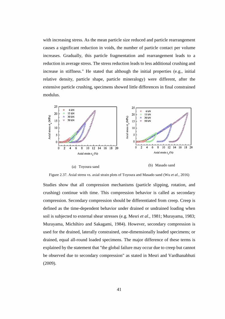
41

with increasing stress. As the mean particle size reduced and particle rearrangement

causes a significant reduction in voids, the number of particle contact per volume

increases. Gradually, this particle fragmentation and rearrangement leads to a

reduction in average stress. The stress reduction leads to less additional crushing and

increase in stiffness." He stated that although the initial properties (e.g., initial

relative density, particle shape, particle mineralogy) were different, after the

extensive particle crushing, specimens showed little differences in final constrained

modulus.

(a) Toyoura sand (b) Masado sand

Figure 2.37. Axial stress vs. axial strain plots of Toyoura and Masado sand (Wu et al., 2016)

Studies show that all compression mechanisms (particle slipping, rotation, and

crushing) continue with time. This compression behavior is called as secondary

compression. Secondary compression should be differentiated from creep. Creep is

defined as the time-dependent behavior under drained or undrained loading when

soil is subjected to external shear stresses (e.g. Mesri et al., 1981; Murayama, 1983;

Murayama, Michihiro and Sakagami, 1984). However, secondary compression is

used for the drained, laterally constrained, one-dimensionally loaded specimens; or

drained, equal all-round loaded specimens. The major difference of these terms is

explained by the statement that "the global failure may occur due to creep but cannot

be observed due to secondary compression" as stated in Mesri and Vardhanabhuti

(2009).

42

Studies on the compression behavior of granular materials show that the compression

index (Cc) changes with effective vertical stress. Particle mineralogy and initial

relative density affect the compression index. Particle shape is also a factor at low

stresses. Chuhan et al. (2003) explain the angularity effects on compression behavior

by stating that angular particles undergo local grain crushing at contact points. This

breakage leads to an increase in contact area and a decrease in contact stresses.

Therefore, the specimen becomes less compressible at higher stresses. In fact, at high

stresses, major effects of grain size, grain shape, grain mineralogy on compression

behavior are observed to disappear. In Figure 2.38, Cc data compiled from literature

by Mesri and Vardhanabhuti (2009) is presented.

Figure 2.38. Cc vs. effective stress plot for different type of sands (Mesri and Vardhanabhuti, 2009)

In addition to the changes in the slope of 𝑒 − 𝑙𝑜𝑔𝜎′𝑣 plot, the slope of 𝑒 − 𝑙𝑜𝑔𝑡 plot

also changes under loading after crushing. The secondary compression index

43

increases with increasing effective stress and becomes significant after the yield

point is passed, and particle crushing (level III) was started (Lade and Liu, 1998).

The mechanism of time-dependent behavior is explained with the particle crushing

in Takei, Kusakabe and Hayashi (2001). Particles are crushed into fragments, and

these fragments are rearranged into a new packing. With this new packing, particle

stresses are re-distributed and reach to a new equilibrium. Then, again particles are

crushed under new re-arranged stress distribution. New fragments are re-arranged

into a new packing, and again, stresses are re-distributed. The crushing process goes

on in this pattern. For angular materials (more specifically, quartz particles in their

study), time-dependent behavior is related to the breakage of angular edges and the

local crushing at contact areas.

2.4.1 Factors Effecting the Particle Breakage

Particle crushing is affected by the initial relative density, gradation, median grain

size, particle mineralogy, particle shape, stress path, and loading type (Roberts and

de Souza, 1958; Hardin, 1985; Hagerty et al., 1993; Nakata, Hyodo, et al., 2001;

Nakata, Kato, et al., 2001).

Initial relative density - Yield stress increases with the increase in initial relative

density, and level III damage is observed at higher 𝜎′𝑣(𝑀𝑀𝑎𝑥). This response is

explained as the particle crushing starting at higher stress levels on the specimens

with higher initial relative density. This behavior is observed due to the lower particle

stress distribution in higher relative density specimens (Roberts and de Souza, 1958;

De Beer, 1963; Coop, 1993; Hagerty et al., 1993; Lade, Yamamuro and Bopp, 1996;

Nakata, Kato, et al., 2001; Chuhan et al., 2003). Therefore, particle breakage

potential decreases with increasing relative density (Hardin, 1985). However,

Chuhan et al. (2003) observed in their study that the loose and dense specimen's

porosity-stress plots are joined and continue together after the yield stress of the

dense specimen has been passed.

44

Gradation - Similar to high relative density specimens, well-graded sands have

higher grain contact; therefore, lower contact stress distribution. Then, they show

higher 𝜎′𝑣(𝑀𝑀𝑎𝑥) than uniformly graded sands (Lade et al., 1996; Nakata, Hyodo,

et al., 2001).

Particle mineralogy – Chuhan et al. (2003) studied the particle mineralogy effect on

compression behavior by using mono-quartz sand, lithic sand, and carbonate sand.

Very coarse-grained chert-rich sand and fine-grained mica-rich sand are also tested.

They stated in their study that chert-rich sands have higher yield stress than other

sands. Carbonate and mica-rich sand have highest porosity loss values at low stresses

(0-5 MPa). Lithic sand, mono-quartz sand, and chert-rich sand follow, respectively,

the carbonate and mica-rich sands in the means of porosity loss. Porosity vs. stress

curves of different sands follow a general trend that the difference between the

curves becomes smaller with increasing grain size, i.e., increasing grain size reduces

the mineralogical effects on compression behavior. After some point, these effects

disappear.

Particle shape - Significant level I and level II particle damage are observed in

angular sands because of the higher tension and shear stresses at interparticle contact

points. This results in lower 𝜎′𝑣(𝑀𝑀𝑎𝑥) values. Hagerty et al. (1993) explain the

behavior with the following hypothesis: There occurs eccentric loading on angular

particles compared to spherical particles. This eccentricity is the reason of the higher

shear and tensile stresses (Hagerty et al., 1993; Lade et al., 1996; McDowell and

Bolton, 1998).

Particle size – The particle breakage potential is proportional to the particle size. It

increases with increasing particle size. This is explained with the same mechanisms,

valid for high relative density and well-graded sands: particle contact forces increase

with particle size. Therefore, breakage increases with size (Hardin, 1985). Chuhan

et al. (2003) studied the grain size effect on compression behavior by using mono-

quartz, lithic, and carbonate sands. At low stresses (0-5 MPa), they observe a small

increase in porosity loss with the increase in grain size. At intermediate stresses (5-

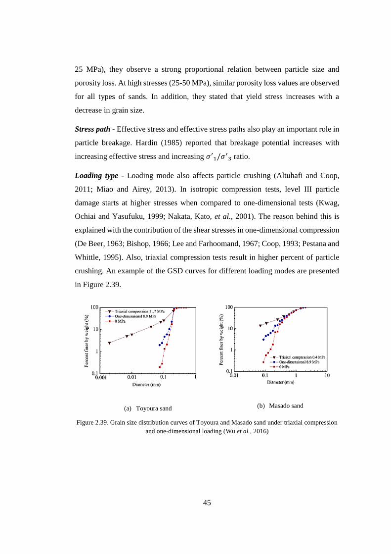
45

25 MPa), they observe a strong proportional relation between particle size and

porosity loss. At high stresses (25-50 MPa), similar porosity loss values are observed

for all types of sands. In addition, they stated that yield stress increases with a

decrease in grain size.

Stress path - Effective stress and effective stress paths also play an important role in

particle breakage. Hardin (1985) reported that breakage potential increases with

increasing effective stress and increasing 𝜎′1/𝜎′

3 ratio.

Loading type - Loading mode also affects particle crushing (Altuhafi and Coop,

2011; Miao and Airey, 2013). In isotropic compression tests, level III particle

damage starts at higher stresses when compared to one-dimensional tests (Kwag,

Ochiai and Yasufuku, 1999; Nakata, Kato, et al., 2001). The reason behind this is

explained with the contribution of the shear stresses in one-dimensional compression

(De Beer, 1963; Bishop, 1966; Lee and Farhoomand, 1967; Coop, 1993; Pestana and

Whittle, 1995). Also, triaxial compression tests result in higher percent of particle

crushing. An example of the GSD curves for different loading modes are presented

in Figure 2.39.

(a) Toyoura sand (b) Masado sand

Figure 2.39. Grain size distribution curves of Toyoura and Masado sand under triaxial compression

and one-dimensional loading (Wu et al., 2016)

46

2.4.2 Particle Breakage Measurements

The amount of particle breakage can be identified from sieve analysis which are

performed on the specimens before and after the compression tests. There are some

measures in the literature to express the amount of breakage quantitatively. Some of

them can be listed as follows;

- Leslie (1963) used the increase in percent passing on sieve size as compared to the

sieve size where original material was 100 % retained

- Later Leslie (1975) again defined a breakage measure as the increase in percent

passing on the sieve size, at which the original material was 90% retained.

- Marsal (1965) defines a breakage measure as the increase in percent passing on the

sieve size, at which the highest increase was observed. However, if increase in

percent passing occurs at more than one diameter, breakage measure is then used as

the sum of these percent passing.

- Lee and Farhoomand (1967) used the D15i/D15a ratio as a breakage measure. D15i is

the diameter of the 15% of the original sample to be finer, and D15a is the diameter

of the 15% of the loaded sample to be finer.

In Figure 2.40, these breakage measurement methods are presented on a GSD graph's

sketch.

47

Figure 2.40. Particle breakage measurements (Hardin, 1985)

Hardin (1985) uses the relative breakage definition as a breakage measure. Relative

breakage (Br) is defined as the ratio of the total breakage to the breakage potential.

All relevant parameters are defined in Eqn. 2-24a through Eqn. 2-27 and Figure 2.41.

𝑏𝑝 = log10 [𝐷 (𝑚𝑚)

0.074] 𝑓𝑜𝑟 𝐷 ≥ 0.074 𝑚𝑚 Eqn. 2-24a

𝑏𝑝 = 0 𝑓𝑜𝑟 𝐷 < 0.074 𝑚𝑚 Eqn 2.24b

𝐵𝑝 = ∫ 𝑏𝑝𝑑𝑓1

0

Eqn. 2-25

𝐵𝑡 = ∫ (𝑏𝑝0 − 𝑏𝑝𝑙)𝑑𝑓1

0

Eqn. 2-26

𝐵𝑟 = 𝐵𝑡/𝐵𝑝 Eqn. 2-27

48

Figure 2.41. Definition of particle breakage measurement suggested by (Hardin, 1985)

2.5 Stiffness of Sandy Soils

Stiffness estimations are listed as one of the important problems in soil mechanics.

The stiffness that was measured in the laboratory, and the one which was back-

calculated from the observations on ground movements in the field, showed

significant differences. Lately, researchers understand these differences in the light

of properties of soil stiffness, especially non-linearity in the behavior (Atkinson,

2000).

Figure 2.42 presents the general stress-strain curves for undrained shearing and

isotropic compression tests.

Figure 2.42. General stress-strain curves for (a) shearing and (b) compression (Atkinson, 2007)

49

Different modulus definitions for different tests are given in Figure 2.43. From

uniaxial loading test Young's modulus, from simple shear test shear modulus, from

isotropic compression test bulk modulus, and from confined compression test

constrained modulus can be estimated.

Figure 2.43. Different modulus types (Lambe and Whitman, 1969)

Basic stiffness parameters from a triaxial test are presented in Figure 2.44. When the

specimen is loaded, a non-linear stress-strain curve is observed, and two different

Young's moduli are defined as the tangent modulus and the secant modulus. Very

small strain, small strain, and large strain levels are defined by Atkinson and Sallfors

(1991). At very small strain level, stiffness reaches to its maximum constant value.

At small strain levels, modulus decreases non-linearly with strain. At larger strain

level, stiffness decreases significantly to a relatively very small value (Atkinson,

2000).

50

Figure 2.44. Basic stiffness parameters (Atkinson, 2000)

The typical stiffness strain curve is an S-shaped curve in the semi-log space and

presented in Figure 2.45. Atkinson (2007) refers the behavior in the very small strain

levels (up to ~0.001%) as linear; hence, stiffness is constant. At small strain level

(in between ~0.001% to ~1%), stress-strain relation is non-linear; therefore, stiffness

decreases with increasing strain increments. At large strains, soil state is on the yield

surface, and elastoplastic behavior is observed. Benz (2007) defines these strain level

boundaries as ~0.0001% and ~0.1% for very small strain and large strain levels,

respectively.

Figure 2.45. Stiffness strain relation (Atkinson, 2007)

51

Typical strain ranges are recommended by Mair (1993) for the structures constructed

in or on London Clay, along with the proper testing technique for different ranges

of strain, as shown in Figure 2.46. Traditional soil tests can be used to observe the

behavior at large strains. Dynamic measurements are needed to measure stiffness at

small strains. The basic method is based on shear wave velocity measurement as

given in Eqn. 2-28. To estimate stiffness at small strain levels, there is a need for the

internal local gauges on the sample to capture very small strain responses, which is

not possible at conventional triaxial tests.

𝐺′0 =𝛾𝑉𝑠

2

𝑔 Eqn. 2-28

Figure 2.46. Typical strain ranges for laboratory tests and typical structures (Atkinson, 2000)

Although the soil is a highly non-linear material, generally, simple analyses are

performed assuming that soil behavior is linear and elastic. A comprehensive

analysis of a geotechnical structure requires special laboratory tests and complex

calculations (Atkinson, 2000).

In Figure 2.47, strength and stiffness relationship of the soil is presented. r, the

reference strain, is defined as the ratio of the peak stress and initial tangent modulus

(Eqn. 2-29). In this figure, solid line presents the non-linear behavior, and the dashed

52

line presents the idealized behavior. Remember that the 𝑞′𝑝 equals to the area under

the stiffness-strain curve from the origin to the peak state. Therefore, the area under

the solid line and the dashed line should be equal as shown in Figure 2.47.

𝜀𝑟 =𝑞′𝑝

𝐸′0 Eqn. 2-29

Figure 2.47. Typical strength-strain and stiffness-strain relation and their idealizations (Atkinson,

2007)

Atkinson (2007) suggests that elastoplastic models, like Cam clay model, can be

used to model soil behavior for large strain levels. He suggests that the Eqn. 2-30

can be used to model the almost linear stress-strain behavior for very small strain

levels. He also suggests that Eqn. 2-31 is suitable to model highly non-linear

response.

𝐺′0

𝑝′𝑟= 𝐴 (

𝑝′

𝑝′𝑟

)

𝑛

𝑌𝑝𝑚 Eqn. 2-30

𝐺′0

𝑝𝑟= 𝐴𝑌𝑝

𝑚 Eqn. 2-31

Lade and Nelson (1987) pointed out that the granular material's response to loading

includes both elastic and plastic straining components. Elastic strains are relatively

small when compared to plastic strains; however, at the initial portion of the stress-

strain relation, an elastic region is observed. Constitutive models need elastic

parameters to cover this elastic response range. Occasionally, elastic models are used

to understand general soil response even at larger strain levels. Thus, although the

53

elastic straining range is small, it cannot be ignored, it should be well-understood

and defined (Lade and Nelson, 1987).

The elastic behavior of granular material is assumed to be isotropic and depends on

the density and stress states of the material. According to Hooke's law, two

independent variables are needed to model the elastic behavior of an isotropic

material from among the following; Poisson's ratio, 𝑣, Young's modulus, 𝐸, bulk

modulus, 𝐵, and shear modulus, 𝐺. The elastic-theory based relations between these

parameters are given in Eqn. 2-32 and Eqn. 2-33.

𝐵 =𝐸

3(1 − 2𝑣) Eqn. 2-32

𝐺 =𝐸

2(1 + 𝑣) Eqn. 2-33

Experimental studies show that the 𝐸, 𝐵 and 𝐺 values depend on the stress state and

Poisson's ratio mostly assumed as constant (Lade and Nelson, 1987).

The initial slope of the stress-strain plot from triaxial compression test or the initial

tangent modulus is the most basic and widely used modulus due to its ease of

estimation from conventional triaxial tests. The modulus relation was originally

proposed by Janbu (1963), which is widely accepted and used. This typical power

function is given as follows:

𝐸 = 𝐾𝑝𝑎 (𝜎3

′

𝑝𝑎)

𝑛

Eqn. 2-34

where 𝐾 is modulus constant, 𝑝𝑎 is atmospheric pressure, 𝜎3′ is confining

stress, and 𝑛 is modulus exponent.

Biarez and Hicher (1994) proposed a relation for Young's modulus as a function of

void ratio, as given in Eqn. 2-35.

54

𝐸0 =140

𝑒√

𝑝′

𝑝𝑟𝑒𝑓 Eqn. 2-35

where 𝑒 is void ratio, 𝑝′ is mean effective stress, 𝑝𝑟𝑒𝑓 is reference stress.

Maximum shear modulus is expressed as functions of confining stress and void ratio

as given in Eqn. 2-36.

𝐺𝑚𝑎𝑥 = 𝐴𝐹(𝑒)𝜎′0𝑛

Eqn. 2-36

where 𝐴 is modulus constant, 𝐹(𝑒) is void ratio function, 𝜎0′ is initial effective

stress, and 𝑛 is modulus exponent.

Hardin and Black (1969) proposed an empirical relation for maximum shear modulus

as given in Eqn. 2-37.

𝐺0 = 33(2.97 − 𝑒)2

1 + 𝑒√

𝑝′

𝑝𝑟𝑒𝑓 Eqn. 2-37

where 𝑒 is void ratio, 𝑝′ is mean effective stress, 𝑝𝑟𝑒𝑓 is reference stress.

There are different modulus relationships and void ratio functions used in the

literature, only a couple of them were presented in this thesis.

55

CHAPTER 3

3 LABORATORY TESTING PROGRAM AND PROCEDURES

3.1 Introduction

In this chapter, the laboratory testing program and testing procedures are described.

The experimental study was carried out on Kızılırmak sand. The laboratory testing

program consists of four soil index tests, 20 monotonic strain-controlled

consolidated undrained triaxial tests, and 7 one-dimensional compression tests.

Triaxial tests and one-dimensional compression tests were performed on relatively

loose and dense, reconstituted sand samples. Kızılırmak sand is a preprocessed in

sand quarry. It is further sieved through No. 4 sieve and coarser fraction is excluded.

Then, it is sieved through No. 200 sieve and the finer fraction is washed out. While

preparing soil samples, the under-compaction method was used for triaxial tests, and

the air pluviation (dry) method was used for one-dimensional compression tests.

3.2 Soil Index Testing and Mineralogy

For Kızılırmak sand, index properties including specific gravity (𝐺𝑠), minimum void

ratio (𝑒𝑚𝑖𝑛), maximum void ratio (𝑒𝑚𝑎𝑥), and gradation were determined. To find

specific gravity (𝐺𝑠), four specimens were prepared, and tests were performed

according to ASTM D854-14. The average 𝐺𝑠 of the Kızılırmak sand was determined

as 2.65. Individual results of all tests are presented in Appendix A.

Maximum void ratio (𝑒𝑚𝑎𝑥) was determined by following the ASTM D4254-16.

Minimum void ratio (𝑒𝑚𝑖𝑛) was determined by vibrating and compressing the soil

into a container in three layers. Experiments were repeated three times for 𝑒𝑚𝑎𝑥 and

two times for 𝑒𝑚𝑖𝑛 determinations. The volume of the container was measured, and

the volume of solids and voids were calculated. 𝑒𝑚𝑎𝑥 was determined as 0.799 and

56

𝑒𝑚𝑖𝑛 was determined as 0.453 by taking the average of the calculated values. The

detailed calculation steps are presented in Appendix B.

Gradation of the Kızılırmak sand was determined by sieve analysis in accordance

with ASTM D6913/6913M-17. Grain size distribution is presented in Figure 3.1. In

this figure, red line represents the average of three experiments. The uniformity

coefficient was determined as 6.07, and the coefficient of curvature was determined

as 0.94. Therefore, according to USCS (Unified Soil Classification System),

Kızılırmak Sand is classified as poorly graded sand. Table 3.1 presents the grain size

characteristics of Kızılırmak Sand.

Particle Size (mm)

0.01 0.1 1 10 100

Per

cen

t F

iner

(%

)

0

20

40

60

80

100

Average GSD curve

Fine Grained Soils Fine Sand Medium Sand Coarse Sand

Figure 3.1. Grain size distribution curves of Kızılırmak sand

57

Table 3.1 Grain size distribution characteristics of Kızılırmak sand

USCS: SP

𝑫𝟏𝟎: 0.22

𝑫𝟑𝟎: 0.54

𝑫𝟓𝟎: 1.01

𝑫𝟔𝟎: 1.36

𝑪𝒖: 6.07

𝑪𝒄: 0.94

Particle mineralogy was also studied for Kızılırmak sand. It was examined using

optical magnification. As a result of this examination, it was observed that

Kızılırmak sand mostly consists of quartz grains, while relatively coarse grains also

include agglomerate and andesite rock fragments (Figure 3.2). Kızılırmak sand

showed a very weak reaction with dilute (10 %) hydrochloric acid. This weak

reaction suggests a minor amount of carbonate minerals in Kızılırmak sand.

Figure 3.2. Agglomerate and andesite rock fragments ( 2 – 3 mm diameter) observed in Kızılırmak

sand

In addition to visual examinations, X-Ray powder diffraction analysis was

performed on Kızılırmak sand which was sieved through no. 40 sieve. X-Ray powder

58

diffraction analysis was performed by METU Civil Engineering Department

Construction Materials Laboratory. XRD pattern of the Kızılırmak sand sample is

given in Figure 3.3. Qualx2 (Altomare et al., 2015) software was utilized to analyse

the XRD pattern and identify main mineral constituents. XRD pattern shows distinct

quartz mineral peaks. Secondary mineral is albite which is a plagioclase feldspar

(mainly Na plagioclase). A minor peak at 29.4o 2-theta indicates a small amount of

calcite mineral.

Figure 3.3. X-Ray powder diffraction pattern and identified minerals of Kızılırmak sand

3.3 Triaxial Testing

The aim of this experimental study is to investigate the volumetric and shear

straining response of Kızılırmak sand. To examine the shear straining response, a

laboratory testing program consisting of 20 monotonic strain-controlled consolidated

undrained triaxial tests with pore water pressure measurement was designed. ASTM

D4767-11 procedure was adopted, although the standard is usually used for cohesive

soils. Due to ease of pore pressure transducer calibration as oppose to volume

transducers, CU tests were preferred as compared to CD tests. Sand specimens were

prepared at various relative densities and consolidated to different cell pressures. The

triaxial testing program is presented in Table 3.2.

59

Table 3.2 Triaxial testing program

Relative Density / Consolidation Pressure

'c=50 kPa 'c=100 kPa 'c=200 kPa 'c=400 kPa

DR = 35 % 35% / 50kPa 35% / 100kPa 35% / 200kPa 35% / 400kPa

DR = 45 % 45% / 50kPa 45% / 100kPa 45% / 200kPa 45% / 400kPa

DR = 60 % 60% / 50kPa 60% / 100kPa 60% / 200kPa 60% / 400kPa

DR = 75 % 75% / 50kPa 75% / 100kPa 75% / 200kPa 75% / 400kPa

DR = 80 % 80% / 50kPa 80% / 100kPa 80% / 200kPa 80% / 400kPa

3.3.1 Sample Preparation

To be able to have homogeneous specimens, reconstituted sand specimen

preparation techniques are generally used in laboratory testing. Ishihara (1996)

suggests three reconstituted sample preparation methods: dry deposition, water

sedimentation, and moist placement.

In the dry deposition method, an oven-dried sand specimen is put into a funnel. Then,

it is poured into the mold through this funnel with zero height and constant velocity.

Target density can be obtained by applying tapping energy by hitting the side of the

mold. By adjusting tapping energy, specimens can be prepared at any density.

In the water sedimentation method, sand is mixed with de-aired water and poured

into the mold with zero height at a constant velocity. In an alternative method, de-

aired water is put into the mold, and dry sand is poured into the mold just above the

water surface. In both water sedimentation methods, it is essential that the sand

deposited under water without considerable sedimentation. If the denser specimen is

aimed, then tapping can be applied by hitting the side of the mold.

In moist placement method, specimen is mixed with de-aired water (about 5%) and

is divided into 5 or 6 equal-weight layers. Each layer of the specimen is poured into

the mold and tamped by a rod. Tamping energy should be arranged considering the

60

target initial density. If a loose specimen is to be prepared, low amount of energy is

needed. If a dense specimen is to be prepared, high amount of energy is needed. This

method allows to prepare a specimen within a wide range of void ratios.

In the moist placement method, it may be hard to apply the same energy to each layer

all the time. Additionally, even though the same energy is applied, due to the

compaction energy transferred from upper layers to lower ones, bottom layers of the

specimen may be over-compacted. To eliminate these problems under-compaction

method is proposed by Ladd (1978). In this method, each layer is compacted to a

lower density than the desired density. This predetermined amount of low

compaction called as percent under-compaction (𝑈𝑛). Percent under-compaction

value increases linearly from the bottom to the top, and it becomes zero at the top

layer. In brief, the bottom layer has the maximum 𝑈𝑛 value and the top layer has

𝑈𝑛=0. Figure 3.4 illustrates the method by using a graph. Percent under-compaction

in a layer is calculated by the following formula;

𝑈𝑛 = 𝑈𝑛𝑖 − [(𝑈𝑛𝑖 − 𝑈𝑛𝑡)

𝑛𝑡 − 1∗ (𝑛 − 1)] Eqn. 3-1

where,

𝑈𝑛𝑖: pecent undercompaction selected for first layer

𝑈𝑛𝑡: pecent undercompaction selected for final layer,usually zero

𝑛: number of layer being considered

𝑛𝑖: first (initial) layer

𝑛𝑡: total numner of layers (final layer)

61

Figure 3.4. Under-compaction method (Ladd, 1978)

The under-compaction method was used as a specimen preparation technique in this

study. Layer number and 𝑈𝑛 values were selected as 10 and 4%, respectively. All

specimens were prepared with a water content of 5%. Required height of each layer

is calculated by;

ℎ𝑛 =ℎ𝑡

𝑛𝑡[(𝑛 − 1) + (1 +

𝑈𝑛

100)] Eqn. 3-2

where,

ℎ𝑡: final (total)height of the specimen

𝑛𝑡: total number of layers

𝑛: number of the layer being considered

𝑈𝑛: percent undercompaction for layer being considered

Required weight of the specimen is calculated by;

𝑊𝑠𝑝𝑒𝑐𝑖𝑚𝑒𝑛 = 𝑊𝑠𝑜𝑙𝑖𝑑𝑠 + 0.05 ∗ 𝑊𝑠𝑜𝑙𝑖𝑑𝑠 Eqn. 3-3

62

𝑊𝑠𝑜𝑙𝑖𝑑𝑠 = 𝐺𝑠 ∗𝑉

1 + 𝑒∗ 𝛾𝑤 Eqn. 3-4

where,

𝑉: volume of specimen (volume of the mold)

𝐺𝑠: specific gravity of the soil,2.65

𝑒: void ratio of the specimen

𝛾𝑤: unit weight of the water

The void ratio at the desired relative density is calculated as:

𝑒 = 𝑒𝑚𝑎𝑥 − 𝐷𝑅 ∗ (𝑒𝑚𝑎𝑥 − 𝑒𝑚𝑖𝑛) Eqn. 3-5

where,

𝑒𝑚𝑎𝑥: maximum void ratio,0.799

𝑒𝑚𝑖𝑛: minimum void ratio,0.453

𝐷𝑅: aimed relative density

3.3.2 Monotonic Triaxial Testing

3.3.2.1 Apparatus

Triaxial tests were performed by using the VJ TECH triaxial testing system shown

in Figure 3.5. The system includes:

A triaxial cell,

A loading-frame,

An automated pressure controller with a pressure transducer to apply and

measure the cell pressure throughout the test,

63

An automated pressure controller with a pressure transducer to apply and

measure the back pressure. In addition, it also measures the volume change

of the specimen throughout the test,

A load cell to measure the deviatoric load acting on the specimen,

A linear variable displacement transducer (LVDT) to measure the axial

deformation of the specimen,

A data logger (MPX3000 with ∓5V range and 16 bits resolution) to monitor

the deviatoric load and axial deformation,

A computer to use Clips software, which controls the automated pressure

control units and allows monitoring the deviatoric load and axial

deformation.

Figure 3.5. VJ TECH triaxial testing system

3.3.2.2 Setup of the specimen

At the beginning of the all experiments, cleaning of the apparatus (soil grains from

the previous experiment were removed from the pedestal with the help of a brush,

back pressure, cell pressure, pore-water pressure, and top cap lines were cleaned by

flushing de-aired water) has been performed. Porous disks were boiled to prevent

64

any blockage in the pores and to eliminate remains from the previous experiment.

Then, a latex membrane was fitted inside the mold, and a filter paper was placed

between the latex membrane and the mold to evenly distribute the suction around the

membrane and protect it from the suction of the vacuum pump. After this, the mold

was connected to the vacuum pump to stretch membrane to mold's wall. In this step,

a vacuum regulator was also connected to the system to control the amount of

vacuum applied to the specimen during specimen preparation. Vacuum regulator is

important to prevent the application of vacuum pressures higher than the

predetermined consolidation pressure. Higher vacuum pressure than the

predetermined consolidation pressure results in an over-consolidated reconstituted

specimen that is not intended for this study. 20 kPa vacuum pressure was used for

the specimens being consolidated to 50 kPa consolidation pressures, and 50 kPa

vacuum pressure is used for the specimens being consolidated to 100 kPa or higher

consolidation pressures. The prepared mold was placed on the pedestal, where

bottom porous disk had already been placed. Prepared mold and vacuuming line is

shown in Figure 3.6.

Figure 3.6. Prepared mold for the experiment

mold

vacuum regulator

vacuum pump

65

The calculated amount of specimen was weighed and mixed with de-aired water to

get ready for the under-compaction process. The specimen amount was decided to

reach to the target relative density. Corresponding equations are provided in Chapter

3.3.1. After adding de-aired water, the specimen was covered with a wet towel to

prevent the loss of water by evaporation. In Figure 3.7, the wetted specimen is

presented.

Figure 3.7. Wetted specimen

As a next step, the specimen was prepared by using the under-compaction method

proposed by Ladd (1978). While applying the method, 10 layers were chosen to get

a more uniform specimen. In this method, soil mass in the layers stays constant, and

layers' heights are changed to achieve predetermined density for that layer. An

adjustable tamping rod, presented in Figure 3.8, was used for this process.

66

Figure 3.8. Tamping rod and caliper

The calculated amount of mass for one layer was taken from the wetted specimen,

and poured into the mold by using a funnel. After that, the soil specimen was

compacted with the tamping rod previously adjusted to the desired height. Then, the

layer's surface was scratched to increase the bond between soil layers. All these

processes are illustrated in Figure 3.9 through Figure 3.14, and are repeated until a

complete sample is prepared. During specimen preparation, it is essential to keep

vacuum pressure constant by using the vacuum regulator.

67

Figure 3.9. Height adjustment of the tamping

rod Figure 3.10. Mass measurement for a layer

Figure 3.11. Measured mass and funnel

68

Figure 3.12. Tamping process Figure 3.13. End of the compaction process

Figure 3.14. Scratching the compacted surface

69

After 10 layers were compacted, top porous stone and top cap were placed on the

specimen. The top cap level was checked by using water gauge in all experiments to

see whether the specimen's surface was flat or not. The flat surface is important to

prevent the loading applied eccentrically. Then, the membrane was fitted to the top

cap, and one of the O-rings from both bottom and top were placed, and then vacuum

pressure was applied to the specimen through the back pressure line. Then, the

second O-rings were placed, and the mold was taken out. The final specimen looks

like the one given in Figure 3.15. Diameter measurements were taken from three

different places of the specimen in different directions. The average of these

measurements was used as a specimen diameter when the volume of the specimen

was calculated.

Figure 3.15. Prepared specimen

After this step, the pedestal was placed on the triaxial setup. The triaxial cell was

placed, and water was filled in it. 20 or 50 kPa cell pressure, according to the

predetermined consolidation pressure, was applied. 20 kPa was used for the

specimens consolidated to 50 kPa consolidation pressure, and 50 kPa was used for

the specimens consolidated to 100 kPa or higher consolidation pressure. During this

process, vacuum pressure was gradually decreased to reach the target effective

70

stresses. After reaching the target cell pressure and decreasing vacuum to zero, the

vacuum pump was disconnected from the setup, and the specimen was ready to

saturation, which will be discussed in the next section.

3.3.2.3 Saturation and Consolidation

Saturation is an essential process for an undrained test to avoid measurement errors

in pore-water pressure. Flushing of de-aired water along with back pressuring were

used in this study to saturate the specimen. To increase the effect of flushing, the

specimen was first flushed with CO2, a gas more soluble than air, before the de-aired

water. Flushing with both CO2 and de-aired water were performed from bottom to

top. The pace of the flushing gas and fluid is important to avoid any undesired

reorientation of the sand grains in the specimen or piping problem. CO2 was applied

for approximately 40 minutes, with the rate of 2-3 bubbles in a minute. The CO2

flushing process can be seen in Figure 3.16 and Figure 3.17.

Figure 3.16. A general view of the CO2 tube and CO2 line

CO2 tube

CO2 line connected to the

bottom of the specimen

71

Figure 3.17. CO2 outlet valve

After CO2, 250-300 ml de-aired water was flushed through the specimen (bottom to

top) to fill voids, as shown in Figure 3.18. In Figure 3.19, bleeding of water from the

specimen top cap can be seen.

Figure 3.18. De-aired water flushing

bubbles due

to CO2

de-aired

water tank

de-aired water

line connected to

the bottom of the

specimen

72

Figure 3.19. Bleeding water from the specimen

During this process, water in the back-pressure water tank was replaced with de-

aired water. After de-aired water flushing was completed, the back pressure

saturation process has begun.

This method takes advantage of the compressibility and solubility of air (CO2 in our

case) in water. Both compressibility and solubility increase with increasing pressure

(Boyle's and Henry's law, respectively). This process has two basic application

methods. In the first one, cell pressure is increased while the drainage line (goes to

specimen) is closed. In the second one, cell pressure and the back pressure in the

specimen are increased simultaneously to keep effective pressure constant. The

second method was preferred and used in this study. Cell and back pressure

increments were adjusted to not over-consolidate the specimen. Therefore, 20 kPa or

50 kPa increments were applied according to predetermined consolidation pressures.

These increments were continued until full saturation was obtained. Saturation was

checked by Skempton's B-value, which is calculated as follows;

de-aired

water bleeding

de-aired water

flushed through

the specimen

73

𝐵 =∆𝑢

∆𝜎3 Eqn. 3-6

where,

∆𝑢: change in pore water pressure

∆𝜎3: change in cell pressure

A B-value of 1 is considered as full saturation. However, one should not forget that

B-value depends on the compressibility of the pore fluid and soil grains. The same

B-value may mean 99% saturation for a stiff soil but only 95% saturation for a soft

soil. Therefore, B-value higher than 95% does not have the same meaning in all

cases. Rather than checking B-value itself, checking its change with pressure may be

more meaningful. When full saturation is achieved, no more change in B-value will

occur. Both B-value itself and its change were monitored in this study.

After each pressure increment, approximately 20-25 minutes was allowed for the

dissolution of the gas in the specimen. Then, the back pressure (drainage) line was

closed, and cell pressure was increased by 20 kPa. The B-value check was done by

dividing the change in pore water pressure by 20 kPa (increase in cell pressure). If

desired B-value and/or change in B-value was not reached, back pressure and cell

pressure was continued to be increased to get the desired B-value. B ≥ 0.93 was

considered to be full saturation for Kızılırmak sand and generally achieved at 500-

600 kPa back pressures.

For the consolidation phase, the back pressure valve was closed, and predetermined

consolidation pressure was applied to the specimen isotropically by increasing the

cell pressure. A few minutes were waited for pore-water pressure stabilization. After

pore-water was stabilized, the consolidation phase was started by opening the

drainage valve. During the consolidation, time vs. volume change data were

recorded. When volume change with time became constant, the consolidation stage

was stopped. For Kızılırmak sand specimens, this took approximately 10 seconds.

The height and the area after consolidation were re-calculated, and in the shearing

74

stage, these updated (corrected) values were used. Axial strain, volumetric strain,

corrected height, and corrected area are calculated by using the Eqn. 3-7 - Eqn. 3-10.

𝜀𝑎 =𝜀𝑣

3 Eqn. 3-7

𝐻𝑐 = 𝐻0 ∗ (1 − 𝜀𝑎) Eqn. 3-8

𝜀𝑣 =∆𝑉

𝑉0 Eqn. 3-9

𝐴𝑐 = 𝐴0 ∗1 − 𝜀𝑣

1 − 𝜀𝑎=

𝑉0 − ∆𝑉

𝐻𝑐 Eqn. 3-10

where,

𝐻𝑐: height of the specimen after consolidation

𝐻0: initial height of the specimen

𝜀𝑎: axial strain

𝜀𝑣: volumetric strain

𝑉0: initial volume of the specimen

∆𝑉: change in volume of the specimen during consolidation stage

𝐴𝑐: area of the specimen after consolidation

𝐴0: initial area of the specimen

3.3.2.4 Monotonic Loading

After the completion of the consolidation stage, the back pressure valve was closed

again to perform the undrained test. The machine shearing rate was set to 1mm/min,

and the last stage of the experiment was started. Applied deviatoric load,

deformation, and pore-water pressure measurements were recorded at every 0.1 mm

75

deformation, and each test was continued to reach to a maximum 15-20% axial

strain.

Before each experiment, the loading rod was lubricated to eliminate the piston

friction. Therefore, piston friction correction was not applied, assuming frictionless

response. To confirm this, at the beginning of shearing, zero force reading was taken

while the axial motor moves at the designated shearing rate without the piston

touching the top cap so that any piston friction and uplift force could be eliminated

during calculations.

Axial strain, deviatoric and mean effective stress, and excess pore-water pressure

were calculated, and four-way plots were prepared for each experiment. The effects

of parabolic and cylindrical area corrections were comparatively tested. It was

concluded that both of the correction schemes produce almost identical failure shear

stresses. However, at larger strains getting close to steady state parabolic area

correction scheme produce approximately 5% smaller shear stresses. Due to their

relative insignificance it was decided to continue with cylindrical area correction

procedure. Therefore, at any stage of shearing, the height and the area of the

specimen were recalculated as given in Eqn. 3-11 through Eqn. 3-13, by assuming

the cylindrical shape of the specimen was not disturbed during the shearing stage.

𝐻𝑐∗ = 𝐻𝑐 − ∆𝐻 Eqn. 3-11

𝐴𝑐∗ =

𝐴𝑐

1 − 𝜀𝑎 Eqn. 3-12

𝜀𝑎 =∆𝐻

𝐻𝑐 Eqn. 3-13

where,

𝐻𝑐∗: height of the specimen after each shearing stage

𝐻𝑐:height of the specimen after consolidation

∆𝐻: axial deformation of the specimen in each shearing stage

76

𝐴𝑐∗ : area of the specimen after each shearing stage

𝐴𝑐: area of the specimen after consolidation

𝜀𝑎: axial strain in each shearing stage

Deviatoric stress, principal effective stresses and half of the deviatoric stress (shear

stress, q) and mean effective stress (p') were calculated by using the following

formulae;

𝜎𝑑 = 𝐹/𝐴𝑐∗ Eqn. 3-14

𝜎′1 = 𝜎𝑐𝑒𝑙𝑙 + 𝜎𝑑 − 𝑢 Eqn. 3-15

𝜎′3 = 𝜎𝑐𝑒𝑙𝑙 − 𝑢 Eqn. 3-16

𝑝′ = (𝜎′1 + 𝜎′

3)/2 Eqn. 3-17

𝑞 = (𝜎′1 − 𝜎′

3)/2 Eqn. 3-18

where,

𝜎𝑑: deviatoric stress

𝐹: force on the specimen

𝜎′1: major effective stress

𝜎′3: minor effective stress

𝜎𝑐𝑒𝑙𝑙: cell pressure

𝑢: pore water pressure

𝑝′: mean effective stress

𝑞: half of deviatoric stress (shear stress)

A sample four way plot is given in Figure 3.20.

77

a (%)

0 5 10 15 20 25

q=

( 1-

3)/

2(k

Pa

)

0

50

100

150

200

250

300

p'=(1'+

3')/2 (kPa) or ' (kPa)

0 50 100 150 200 250 300

q=

( 1-

3)/

2 (

kP

a)

or

(

kP

a)

0

50

100

150

200

250

300

a (%)

0 5 10 15 20 25

Uex

c (k

Pa

)

-40

-30

-20

-10

0

10

20

30

p'=(1'+

3')/2 (kPa)

0 50 100 150 200 250 300

q/p

'

0.0

0.1

0.2

0.3

0.4

0.5

0.6

0.7

a= 1.5 %

@ q= 41.3 kPa

=36.2o

@ q= 41.3 kPa

q/p'= 0.59

@ p'= 70.0 kPa

Uexc

= 19.0 kPa

@ a= 1.5 %

Figure 3.20. An example of four-way plot (TRX_45-50)

3.4 One-Dimensional Compression Test

To examine the volumetric straining response, a laboratory testing program,

consisting of 7 oedometer tests was designed. Sand specimens were prepared at 25-

35-45-60-75-80-85 % relative densities, and loaded up to an axial stress of ~33.5

MPa. ASTM D2435/D2435M-11 procedure was adopted, although the standard is

widely used for cohesive soils.

78

3.4.1 Sample Preparation

To be able to get homogeneous specimens, reconstituted sand specimen preparation

techniques were used as part of the laboratory testing program. The dry deposition

method was preferred for one-dimensional testing. In this method, an oven-dried

specimen was placed into a funnel. Then, the soil was poured into the mold through

this funnel at zero dropping height and constant velocity. Target density is obtained

by applying tapping energy, hitting the side of the mold. By adjusting tapping energy,

specimens can be prepared at target densities (Ishihara, 1996).

Required weight of the specimen was calculated as:

𝑊𝑠𝑜𝑖𝑙 = 𝐺𝑠 ∗𝑉

1 + 𝑒 Eqn. 3-19

where,

𝑉: volume of specimen (volume of the mold)

𝐺𝑠: specific gravity of the soil,2.65

𝑒: void ratio of the specimen

The void ratio at the desired relative density was calculated as:

𝑒 = 𝑒𝑚𝑎𝑥 − 𝐷𝑅 ∗ (𝑒𝑚𝑎𝑥 − 𝑒𝑚𝑖𝑛) Eqn. 3-20

where,

𝑒𝑚𝑎𝑥: maximum void ratio,0.799

𝑒𝑚𝑖𝑛: minimum void ratio,0.453

𝐷𝑅: target relative density

79

3.4.2 One-Dimensional Compression Testing Procedure

3.4.2.1 Apparatus

One-dimensional compression tests were performed by using the SOILTEST

oedometer apparatus and a data acquisition system, shown in Figure 3.21. The

system includes:

An oedometer apparatus with loading frame and two levels of the lever arm

to apply the load on the specimen,

An oedometer mold with a diameter of 50 mm to prepare the specimen,

21 metal weights, ranging from ~250 gr. up to ~16 kg., to load the specimen,

A linear variable displacement transducer (LVDT) to measure the axial

deformation of the specimen,

A data acquisition system (TestBOX1001 with ∓10V range and 16 bit

resolution) to monitor axial deformations,

A computer where Test Lab software and the axial deformation data were

installed and saved, respectively.

Figure 3.21. SOILTEST oedometer apparatus and data acquisition system

80

The oedometer apparatus used for the experiments has two loading posts. One has

an overall load magnification of 1:10 lever ratio, and the other 1:40, as shown in

Figure 3.22.

Figure 3.22. SOILTEST oedometer apparatus' lever ratios

3.4.2.2 Loading

Both of the two hangers discussed previously were used during the experiments.

First, the 1:10 lever ratio part of the apparatus was used to apply relatively small

pressures on the specimen. Then, the 1:40 lever ratio part was used for higher

stresses. During loading, at selected point, reloading was performed, and then the

test was continued with loading again. Five loading and unloading cycles were

performed on each test. A total of 41 loadings were applied as part of these 5 cycles.

The predetermined loading pattern is presented in Table 3.3. In this table, the black

1 unit

8 units

1 unit

5 units

2 units

81

font represents loading, whereas the red and italic font unloading. Applied loads on

specimens were calculated by using the 1:10 and 1:40 lever ratios. T

able

3.3

On

e-d

imen

sio

nal

tes

t lo

adin

g i

ncr

emen

ts

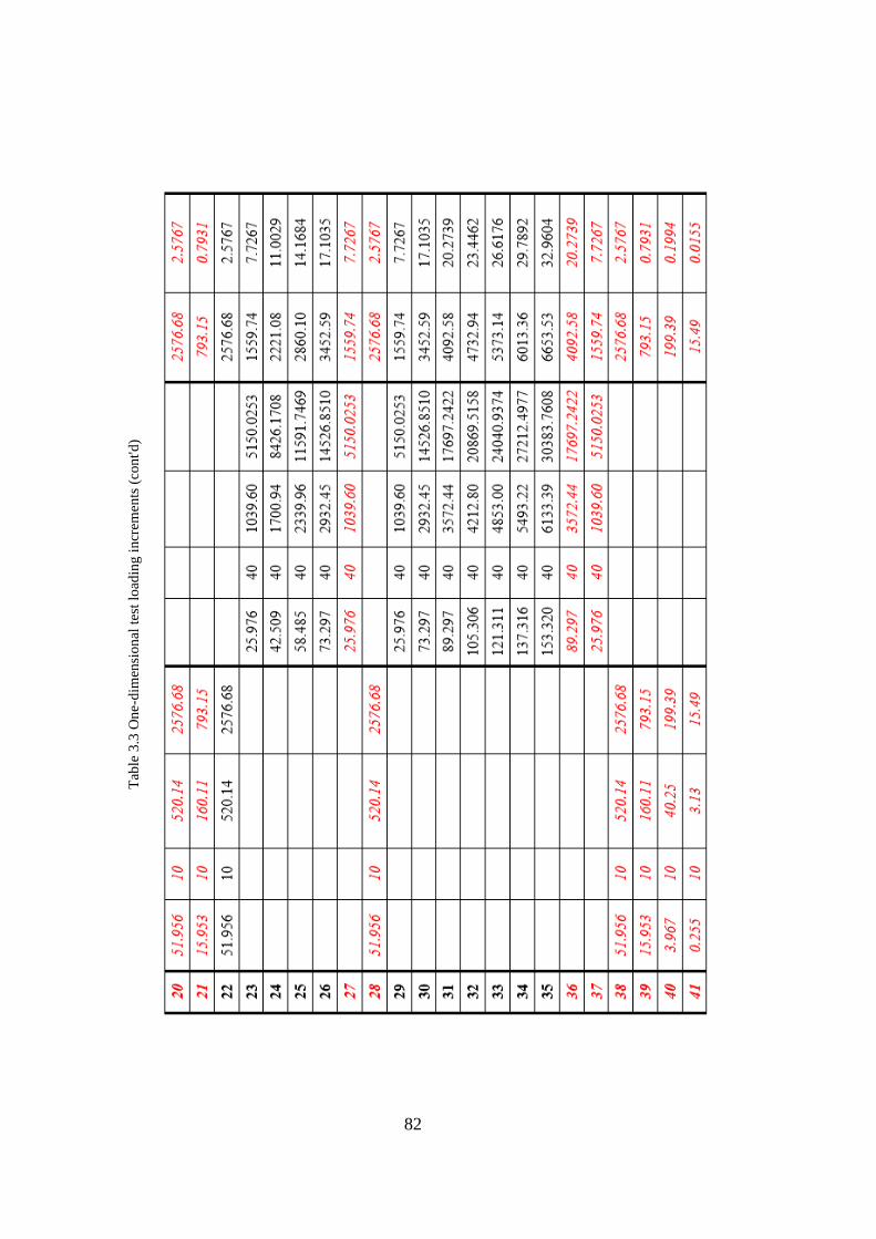
82

Tab

le 3

.3 O

ne-

dim

ensi

on

al t

est

load

ing

in

crem

ents

(co

nt'd

)

83

3.4.2.3 Loading weights and oedometer lever ratio calibration

In order to check the ratio of the lever arm and to confirm that the loads were applied

accurately and precisely, a calibration scheme was followed by using a calibrated

load cell. For this process, a load cell was placed into the cell, in the place of the

specimen.

A load cell, which has a 10 ton capacity was used for the calibration process. It was

loaded in the pattern given in Table 3.3 without any inter-reloading pattern. Three

loading and unloading cycles were performed. The calibration line for the 1:40 lever

ratio is presented in Figure 3.23. In order to avoid the non-linearity in the smaller

loads, another load cell with a smaller capacity was used. Loads up to 520 kg were

calibrated by this 1-ton capacity load cell. It was loaded in the load pattern of the

load number 1-4, 9-11, 16-17 (i.e., up to ~500 kg on the specimen but without any

inter-reloading) given in Table 3.3. Loading and unloading cycles were performed 3

times. The calibration line is presented in Figure 3.24. Figure 3.23 and Figure 3.24

confirm the 1:40 and 1:10 lever ratios of the apparatus.

Figure 3.23. Calibration line for the load higher

than ~500 kg Figure 3.24. Calibration line for the load

smaller than ~500 kg

84

In conclusion, true loads were estimated as given in Table 3.4.

Table 3.4 Comparison of calculated and calibrated loads

Load on

×10

(kg)

Load on

×40

(kg)

Calculated

Load

on Specimen

(kg)

Calculated

Pressure

(MPa)

True Load

on

Specimen

(kg)

True

Pressure

(MPa)

0.255 2.55 0.0126 3.38 0.0170

0.510 5.10 0.0253 5.99 0.0301

0.967 9.67 0.0479 10.66 0.0536

1.970 19.70 0.0976 20.91 0.1052

3.967 39.67 0.1965 41.31 0.2078

7.956 79.56 0.3941 82.07 0.4129

15.953 159.53 0.7903 163.77 0.8239

31.958 319.58 1.5831 327.29 1.6466

51.956 519.56 2.5738 531.61 2.6746

10.004 919.71 4.5561 969.87 4.8794

25.976 1558.59 7.7210 1603.76 8.0685

42.509 2219.93 10.9971 2259.93 11.3697

58.485 2858.94 14.1627 2893.95 14.5595

73.297 3451.43 17.0978 3481.82 17.5171

89.297 4091.42 20.2682 4116.81 20.7117

105.306 4731.79 23.4405 4752.17 23.9082

121.3106 5371.99 26.6119 5387.36 27.1039

137.3162 6012.21 29.7835 6022.59 30.2997

153.3203 6652.37 32.9547 6657.75 33.4952

85

3.4.2.4 Machine deflection calculations

To eliminate the displacements due to machine deflection/seating during testing,

four tests were performed, without sand samples inplace. The oedometer apparatus

was loaded following the same loading pattern; however, a sand specimen was not

placed into the mold. Therefore, measured deformations were uniquely due to

machine deflection/seating.

Figure 3.25. Machine deflections as compared with some oedometer tests performed on Kızılırmak

sand

A comparison of the machine deflection/seating deformation and oedometer test data

with Kızılırmak sand is presented in Figure 3.25. As can be seen from Figure 3.25,

machine deflection/seating deformation values are very small compared to sand

deformations, and all four tests gave slightly different deflection results. Therefore,

it was concluded that there exists some randomness in machine deflections and their

measurements. This could be due to their relatively low magnitude and intrinsic

variabilities in machine preparations. The average of these results was used as

machine deflection/seating deformation data, and subtracted from oedometer test

86

data with Kızılırmak sand samples inplace. This average is presented in Figure 3.25

by a red line.

3.4.2.5 Setup of the specimen

At the beginning of all experiments, cleaning of the mold, especially top cap, from

the crushed material which could be stuck in the metal joints, has been performed.

Then, the required mass of sand specimen was calculated and put into the mold with

the help of a spoon and funnel. After pouring sand into the mold, vibration was

applied by using a metal rod to reach to the target relative density. After tapping, the

top cap was placed, and the flatness of the specimen's surface was checked by a water

level. These procedures are shown in Figure 3.26 through Figure 3.28.

Figure 3.26. Pieces of equipment used for specimen preparation; a bowl, balance, spoon, funnel,

oedometer mold and top cap

87

Figure 3.27. Dry pluviation process and the sample after the completion of pluviation

Figure 3.28. Tapping and checking the flatness of the specimen's surface

88

After the specimen is prepared, the mold was placed on the oedometer apparatus,

and the load frame's height was adjusted to touch the top cap with applying zero load

on the specimen, as shown in Figure 3.29. Then, LVDT was placed on the load frame

to measure the axial deformations. After the completion of these procedures, the

specimen was ready for loading. At the end of each experiment, the specimen was

saved in a bag to perform sieve analysis. In Figure 3.29 through Figure 3.33, LVDT

placement, apparatus under maximum load, and removal process of the specimen

can be seen.

Figure 3.29. Placement of the prepared specimen under the loading frame

Figure 3.30. Placement of the LVDT on the loading frame

89

Figure 3.31. Apparatus under maximum load

Figure 3.32. A view of the specimen after the test

Figure 3.33. Removing specimen from the mold

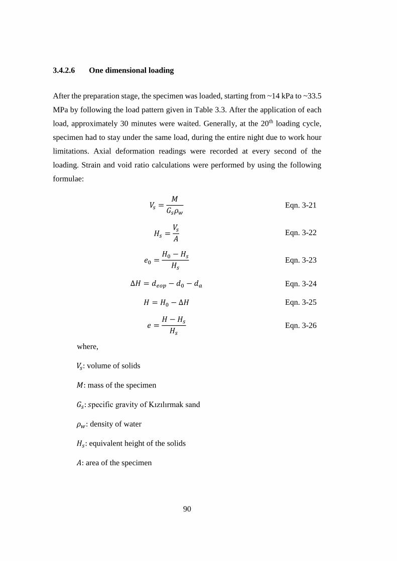
90

3.4.2.6 One dimensional loading

After the preparation stage, the specimen was loaded, starting from ~14 kPa to ~33.5

MPa by following the load pattern given in Table 3.3. After the application of each

load, approximately 30 minutes were waited. Generally, at the 20th loading cycle,

specimen had to stay under the same load, during the entire night due to work hour

limitations. Axial deformation readings were recorded at every second of the

loading. Strain and void ratio calculations were performed by using the following

formulae:

𝑉𝑠 =𝑀

𝐺𝑠𝜌𝑤 Eqn. 3-21

𝐻𝑠 =𝑉𝑠

𝐴 Eqn. 3-22

𝑒0 =𝐻0 − 𝐻𝑠

𝐻𝑠 Eqn. 3-23

∆𝐻 = 𝑑𝑒𝑜𝑝 − 𝑑0 − 𝑑𝑎 Eqn. 3-24

𝐻 = 𝐻0 − ∆𝐻 Eqn. 3-25

𝑒 =𝐻 − 𝐻𝑠

𝐻𝑠 Eqn. 3-26

where,

𝑉𝑠: volume of solids

𝑀: mass of the specimen

𝐺𝑠: 𝑠pecific gravity of Kızılırmak sand

𝜌𝑤: density of water

𝐻𝑠: equivalent height of the solids

𝐴: area of the specimen

91

𝑒0: initial void ratio of the specimen

𝐻0: initial height of the specimen

∆𝐻: change in specimen height at the end of primary consolidation

𝑑𝑒𝑜𝑝: deformation reading in each loading stage at the end of

primary compression

𝑑0: initial deformation reading in each loading stage

𝑑𝑎: apparatus deformation in each stage

𝐻: height of the specimen at the end of primary consolidation

𝑒: void ratio of the specimen at the end of primary consolidation

𝜀 =∆𝐻

𝐻0∗ 100 Eqn. 3-27

where,

𝜀: axial strain at the end of primary consolidation

𝜎𝑎 = (𝑃 + 𝑀𝑎 ∗ 𝑔

𝐴) Eqn. 3-28

where,

𝜎𝑎: axial stress

𝑃: load acting on the specimen

𝑀𝑎: mass of the top cap

𝑔: acceleration due to gravity, 9.81 m/s2

𝐴: area of the specimen

The end of primary compression displacement (𝑑𝑒𝑜𝑝) was calculated by drawing

axial deformation vs. logarithm of the time plot as suggested by Casagrande (1963).

However, the procedure was adopted to sand's behavior by taking the interception of

92

two linear parts of deformation vs. log-time graph as the end of the primary

compression value. At high pressures, after crushing was occurred, this method could

not be applied due to the highly creeping response of the crushed sand. For these

pressures, displacement vs. square root of time graph was plotted as recommended

by Taylor (1948). The end of primary consolidation value (𝑑100) defined in Taylor's

method was taken as the end of primary compression (𝑑𝑒𝑜𝑝). Primary compression

ended in 2 to 10 seconds after loading. This is illustrated in in Figure 3.34.

Figure 3.34. Example plots for determination of end of primary compression

Tangent compression and recompression indices and constrained moduli were

calculated by using the following formulae:

𝐶𝑐 𝑜𝑟 𝐶𝑟 =∆𝑒

∆𝑙𝑜𝑔𝜎′𝑣 Eqn. 3-29

𝑀 =∆𝜎′𝑣

∆𝜀𝑎 Eqn. 3-30

where,

𝐶𝑐: tangent compression index

𝐶𝑟: tangent recompression index

𝑀: tangent constrained modulus

∆𝑒: change in void ratio

93

∆𝜎′𝑣: change in axial stress

∆𝜀𝑎: change in axial strain

Secondary compression index was calculated by Eqn. 3-31.

𝐶𝛼 =∆𝑒

∆𝑙𝑜𝑔𝑡 Eqn. 3-31

where,

𝐶𝛼: secondary compression index

95

CHAPTER 4

4 TEST RESULTS AND THEIR INTERPRETATIONS

4.1 Introduction

In this chapter, results of CU-triaxial and oedometer tests are presented and

compared with the available literature. For this purpose, four-way plots were

prepared to illustrate the response of Kızılırmak sand under shear straining. Also, to

examine the relative density and confining stress effects on the shearing response

and strength, comparative graphs were prepared. For the oedometer tests, e vs. log'v

graphs were prepared. Constrained modulus, compression index, secondary

compression index, and yield stress were calculated corresponding to different stress

levels and relative densities.

4.2 CU Monotonic Triaxial Test Results

In Table 4.1, initial relative density (𝐷𝑅), initial void ratio (𝑒0), consolidation

pressure (𝜎′𝑐), void ratio after consolidation (𝑒𝑐), axial strain value at failure

(𝜀𝑎,𝑓𝑎𝑖𝑙𝑢𝑟𝑒) and effective stress angle of shearing resistance (𝜙′) are summarized.

96

Table 4.1 Summary of the triaxial test results

Test Name 𝑫𝑹(%) 𝒆𝟎 𝝈′𝒄 (𝒌𝑷𝒂) 𝒆𝒄 𝜺𝒂,𝒇𝒂𝒊𝒍𝒖𝒓𝒆 (%) 𝝓′(°)

TRX_35-50 34 0.681 53.5 0.672 1.3 36.4

TRX_35-100 35 0.678 97.6 0.657 2.0 36.3

TRX_35-200 36 0.674 97.6 0.640 2.0 35.4

TRX_35-400 34 0.682 398.9 0.612 4.1 38.7

TRX_45-50 46 0.641 47.7 0.634 1.5 36.2

TRX_45-100 45 0.643 88.8 0.624 2.0 36.4

TRX_45-200 47 0.636 203.1 0.607 2.0 37.8

TRX_45-400 47 0.636 397.7 0.590 2.6 40.2

TRX_60-50 59 0.595 50.7 0.589 0.8 40.5

TRX_60-100 60 0.591 99.3 0.577 1.1 40.4

TRX_60-200 60 0.592 191.8 0.567 1.5 39.2

TRX_60-400 59 0.594 399.9 0.558 2.1 39.8

TRX_75-50 74 0.544 52.6 0.538 0.9 42.3

TRX_75-100 72 0.550 96.9 0.539 1.0 41.6

TRX_75-200 73 0.545 184.5 0.524 1.3 41.0

TRX_75-400 73 0.547 402.7 0.519 1.8 40.6

TRX_80-50 81 0.519 53.8 0.514 1.2 43.7

TRX_80-100 83 0.512 94.0 0.499 0.9 43.5

TRX_80-200 83 0.511 199.8 0.486 1.5 42.8

TRX_80-400 82 0.516 400.7 0.486 1.5 41.9

97

Half of the deviatoric stress (shear stress) vs. axial strain (q vs. 𝜀𝑎), half of the

deviatoric stress (shear stress) vs. mean effective stress (q vs. p'), shear stress vs.

effective stress (𝜏 vs. 𝜎′), excess pore water pressure vs. axial strain (Uexc vs. 𝜀𝑎),

effective stress ratio (stress obliquity) vs. mean effective stress (q/p' vs. p') graphs

are presented in the form of four-way plots. Failure point was estimated benefitting

from maximum obliquity criterion, and these points are shown in the graphs

mentioned above. Four-way plots of each CU triaxial test are presented in Figure 4.1

through Figure 4.20.

a (%)

0 5 10 15 20 25

q=

( 1-

3)/

2 (

kP

a)

0

20

40

60

80

100

120

140

p'=(1'+

3')/2 (kPa) or ' (kPa)

0 20 40 60 80 100 120 140

q=

( 1-

3)/

2 (

kP

a)

or

(

kP

a)

0

20

40

60

80

100

120

140

a (%)

0 5 10 15 20 25

Uex

c (k

Pa

)

0

5

10

15

20

25

p'=(1'+

3')/2 (kPa)

0 20 40 60 80 100 120 140

q/p

'

0.0

0.1

0.2

0.3

0.4

0.5

0.6

0.7

a= 1.3 %

@ q= 40.5 kPa

=36.4o

@ q= 40.5 kPa

q/p'= 0.59

@ p'= 68.3 kPa

Uexc

= 21.2 kPa

@ a= 1.3 %

Figure 4.1. Four-way plots of TRX_35-50

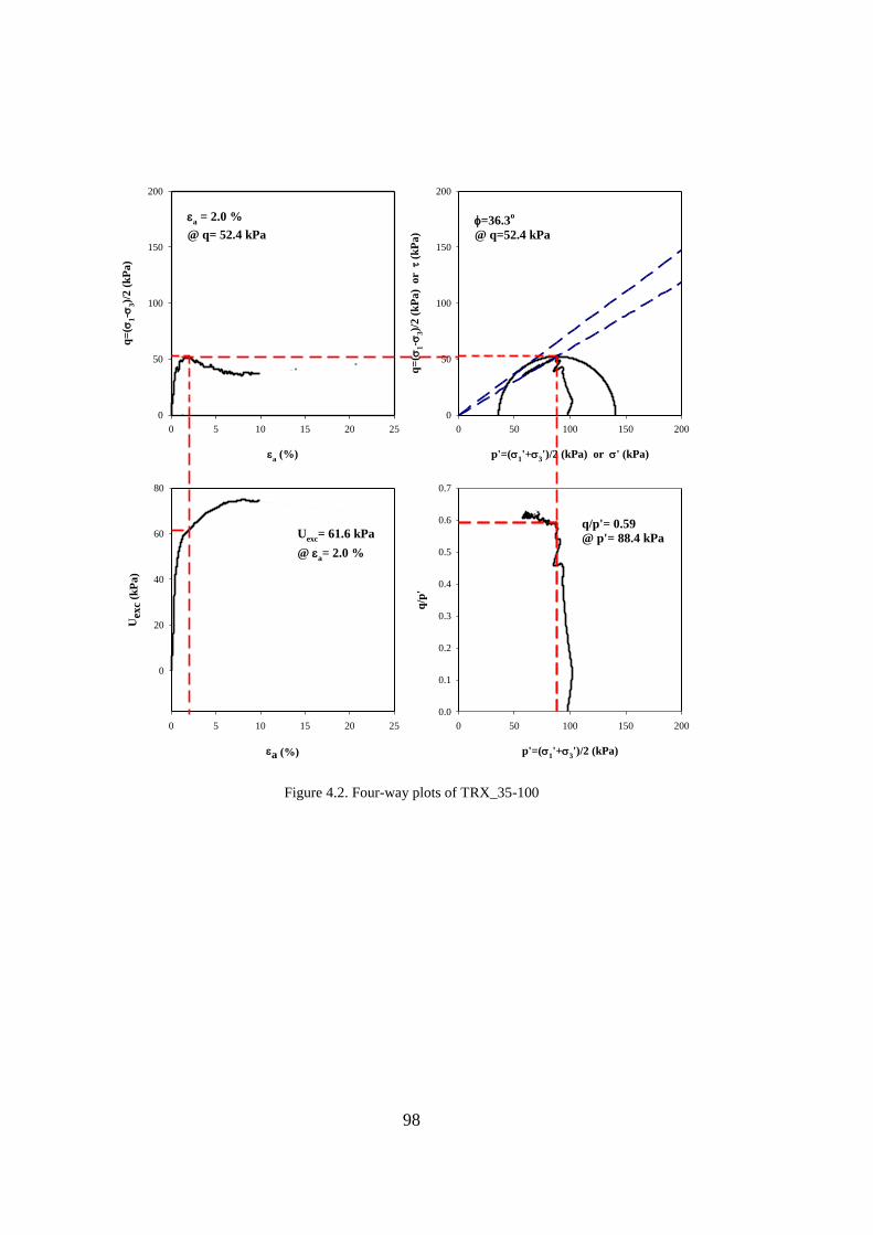
98

a (%)

0 5 10 15 20 25

q=

( 1-

3)/

2 (

kP

a)

0

50

100

150

200

p'=(1'+

3')/2 (kPa) or ' (kPa)

0 50 100 150 200

q=

( 1-

3)/

2 (

kP

a)

or

(

kP

a)

0

50

100

150

200

a (%)

0 5 10 15 20 25

Uex

c (k

Pa

)

0

20

40

60

80

p'=(1'+

3')/2 (kPa)

0 50 100 150 200

q/p

'

0.0

0.1

0.2

0.3

0.4

0.5

0.6

0.7

a = 2.0 %

@ q= 52.4 kPa

=36.3o

@ q=52.4 kPa

q/p'= 0.59

@ p'= 88.4 kPaUexc

= 61.6 kPa

@ a= 2.0 %


99

a (%)

0 5 10 15 20 25 30

q=

( 1-

3)/

2 (

kP

a)

0

50

100

150

200

250

300

p'=(1'+

3')/2 (kPa) or ' (kPa)

0 50 100 150 200 250 300

q=

( 1-

3)/

2 (

kP

a)

or

(

kP

a)

0

50

100

150

200

250

300

a (%)

0 5 10 15 20 25 30

Uex

c (k

Pa

)

0

20

40

60

80

100

120

140

160

p'=(1'+

3')/2 (kPa)

0 50 100 150 200 250 300

q/p

'

0.0

0.1

0.2

0.3

0.4

0.5

0.6

0.7

a= 2.0 %

@ q= 98.4 kPa

=35.4o

@ q= 98.4 kPa

q/p'= 0.58 kPa

@ p'= 170.0 kPaU

exc= 130.5 kPa

@ a= 2.0 %


100

a (%)

0 5 10 15 20 25

q=

( 1-

3)/

2 (

kP

a)

0

100

200

300

400

500

600

p'=(1'+

3')/2 (kPa) or ' (kPa)

0 100 200 300 400 500 600

q=

( 1-

3)/

2 (

kP

a)

or

(

kP

a)

0

100

200

300

400

500

600

a (%)

0 5 10 15 20 25

Uex

c (k

Pa

)

0

50

100

150

200

250

300

350

p'=(1'+

3')/2 (kPa)

0 100 200 300 400 500 600

q/p

'

0.0

0.1

0.2

0.3

0.4

0.5

0.6

0.7

a= 4.1 %

@ q= 184.2 kPa

=38.7o

@ q= 184.2kPa

q/p'= 0.62 kPa

@ p'= 294.9 kPaU

exc= 288.2 kPa

@ a= 4.1 %


101

a (%)

0 5 10 15 20 25

q=

( 1-

3)/

2(k

Pa

)

0

50

100

150

200

250

300

p'=(1'+

3')/2 (kPa) or ' (kPa)

0 50 100 150 200 250 300

q=

( 1-

3)/

2 (

kP

a)

or

(

kP

a)

0

50

100

150

200

250

300

a (%)

0 5 10 15 20 25

Uex

c (k

Pa

)

-40

-30

-20

-10

0

10

20

30

p'=(1'+

3')/2 (kPa)

0 50 100 150 200 250 300

q/p

'

0.0

0.1

0.2

0.3

0.4

0.5

0.6

0.7

a= 1.5 %

@ q= 41.3 kPa

=36.2o

@ q= 41.3 kPa

q/p'= 0.59

@ p'= 70.0 kPa

Uexc

= 19.0 kPa

@ a= 1.5 %


102

a (%)

0 5 10 15 20 25

q=

( 1-

3)/

2 (

kP

a)

0

50

100

150

200

250

300

p'=(1'+

3')/2 (kPa) or ' (kPa)

0 50 100 150 200 250 300

q=

( 1-

3)/

2 (

kP

a)

or

(

kP

a)

0

50

100

150

200

250

300

a (%)

0 5 10 15 20 25

Uex

c (k

Pa

)

-40

-20

0

20

40

60

p'=(1'+

3')/2 (kPa)

0 50 100 150 200 250 300

q/p

'

0.0

0.1

0.2

0.3

0.4

0.5

0.6

0.7

a = 2.0 %

@ q= 58.0 kPa

=36.4o

@ q=58.0 kPa

q/p'= 0.57

@ p'= 97.8 kPa

Uexc

= 49.8 kPa

@ a= 2.0 %


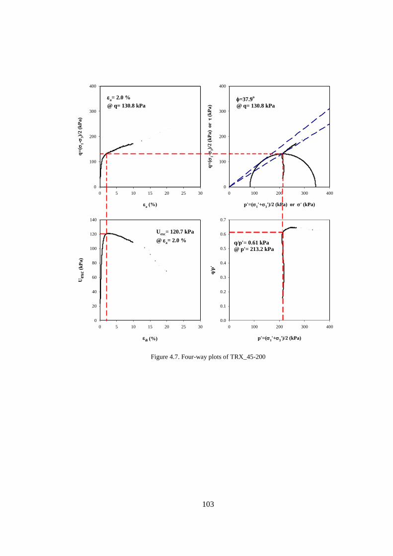
103

a (%)

0 5 10 15 20 25 30

q=

( 1-

3)/

2 (

kP

a)

0

100

200

300

400

p'=(1'+

3')/2 (kPa) or ' (kPa)

0 100 200 300 400

q=

( 1-

3)/

2 (

kP

a)

or

(

kP

a)

0

100

200

300

400

a (%)

0 5 10 15 20 25 30

Uex

c (k

Pa

)

0

20

40

60

80

100

120

140

p'=(1'+

3')/2 (kPa)

0 100 200 300 400

q/p

'

0.0

0.1

0.2

0.3

0.4

0.5

0.6

0.7

a= 2.0 %

@ q= 130.8 kPa

=37.9o

@ q= 130.8 kPa

q/p'= 0.61 kPa

@ p'= 213.2 kPa

Uexc

= 120.7 kPa

@ a= 2.0 %


104

a (%)

0 5 10 15 20 25

q=

( 1-

3)/

2 (

kP

a)

0

200

400

600

800

p'=(1'+

3')/2 (kPa) or ' (kPa)

0 200 400 600 800

q=

( 1-

3)/

2 (

kP

a)

or

(

kP

a)

0

200

400

600

800

a (%)

0 5 10 15 20 25

Uex

c (k

Pa

)

0

50

100

150

200

250

p'=(1'+

3')/2 (kPa)

0 200 400 600 800

q/p

'

0.0

0.2

0.4

0.6

0.8

a= 2.6 %

@ q= 304.9 kPa

=40.2o

@ q= 304.9 kPa

q/p'= 0.65 kPa

@ p'= 472.4 kPaU

exc= 230.2 kPa

@ a= 2.6 %


105

a (%)

0 5 10 15 20 25

q=

( 1-

3)/

2 (

kP

a)

0

100

200

300

400

p'=(1'+

3')/2 (kPa) or ' (kPa)

0 100 200 300 400

q=

( 1-

3)/

2 (

kP

a)

or

(

kP

a)

0

100

200

300

400

a (%)

0 5 10 15 20 25

Uex

c (k

Pa

)

-120

-100

-80

-60

-40

-20

0

20

p'=(1'+

3')/2 (kPa)

0 100 200 300 400

q/p

'

0.0

0.2

0.4

0.6

0.8

a= 0.80 %

@ q= 76.3 kPa

=40.5o

@ q= 76.3 kPa

q/p'= 0.65

@ p'= 117.6 kPa

Uexc

= 9.4 kPa

@ a= 0.80 %


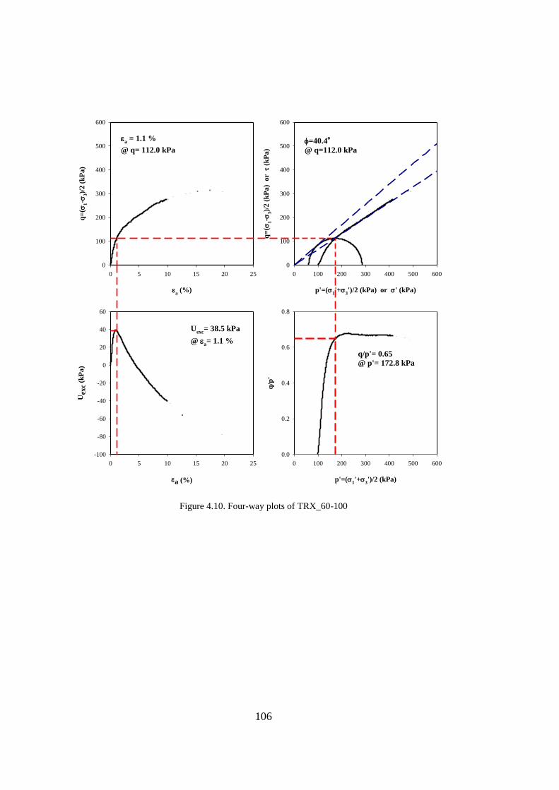
106

a (%)

0 5 10 15 20 25

q=

( 1-

3)/

2 (

kP

a)

0

100

200

300

400

500

600

p'=(1'+

3')/2 (kPa) or ' (kPa)

0 100 200 300 400 500 600

q=

( 1-

3)/

2 (

kP

a)

or

(

kP

a)

0

100

200

300

400

500

600

a (%)

0 5 10 15 20 25

Uex

c (k

Pa

)

-100

-80

-60

-40

-20

0

20

40

60

p'=(1'+

3')/2 (kPa)

0 100 200 300 400 500 600

q/p

'

0.0

0.2

0.4

0.6

0.8

a = 1.1 %

@ q= 112.0 kPa

=40.4o

@ q=112.0 kPa

q/p'= 0.65

@ p'= 172.8 kPa

Uexc

= 38.5 kPa

@ a= 1.1 %


107

a (%)

0 5 10 15 20 25 30

q=

( 1-

3)/

2 (

kP

a)

0

100

200

300

400

500

600

p'=(1'+

3')/2 (kPa) or ' (kPa)

0 100 200 300 400 500 600

q=

( 1-

3)/

2 (

kP

a)

or

(

kP

a)

0

100

200

300

400

500

600

a (%)

0 5 10 15 20 25 30

Uex

c (k

Pa

)

0

20

40

60

80

100

120

p'=(1'+

3')/2 (kPa)

0 100 200 300 400 500 600

q/p

'

0.0

0.1

0.2

0.3

0.4

0.5

0.6

0.7

a= 1.5 %

@ q= 163.6 kPa

=39.2o

@ q= 163.6 kPa

q/p'= 0.63 kPa

@ p'= 259.1 kPa

Uexc

= 96.3 kPa

@ a= 1.5 %


108

a (%)

0 5 10 15 20 25

q=

( 1-

3)/

2 (

kP

a)

0

200

400

600

800

p'=(1'+

3')/2 (kPa) or ' (kPa)

0 200 400 600 800

q=

( 1-

3)/

2 (

kP

a)

or

(

kP

a)

0

200

400

600

800

a (%)

0 5 10 15 20 25

Uex

c (k

Pa

)

0

50

100

150

200

250

300

p'=(1'+

3')/2 (kPa)

0 200 400 600 800

q/p

'

0.0

0.1

0.2

0.3

0.4

0.5

0.6

0.7

a= 2.1 %

@ q= 278.3 kPa

=39.8o

@ q= 278.3 kPa

q/p'= 0.64 kPa

@ p'= 434.5 kPa

Uexc

= 243.7 kPa

@ a= 2.1 %


109

a (%)

0 5 10 15 20 25

q=

( 1-

3)/

2 (

kP

a)

0

200

400

600

800

p'=(1'+

3')/2 (kPa) or ' (kPa)

0 200 400 600 800

q=

( 1-

3)/

2 (

kP

a)

or

(

kP

a)

0

200

400

600

800

a (%)

0 5 10 15 20 25

Uex

c (k

Pa

)

-250

-200

-150

-100

-50

0

50

p'=(1'+

3')/2 (kPa)

0 200 400 600 800

q/p

'

0.0

0.2

0.4

0.6

0.8

a= 0.94 %

@ q= 59.6 kPa

=42.3o

@ q= 59.6 kPa

q/p'= 0.67

@ p'= 88.5 kPa

Uexc

= 23.7 kPa

@ a= 0.94 %


110

a (%)

0 5 10 15 20 25

q=

( 1-

3)/

2 (

kP

a)

0

200

400

600

800

p'=(1'+

3')/2 (kPa) or ' (kPa)

0 200 400 600 800

q=

( 1-

3)/

2 (

kP

a)

or

(

kP

a)

0

200

400

600

800

a (%)

0 5 10 15 20 25

Uex

c (k

Pa

)

-140

-120

-100

-80

-60

-40

-20

0

20

40

60

p'=(1'+

3')/2 (kPa)

0 200 400 600 800

q/p

'

0.0

0.2

0.4

0.6

0.8

a = 1.0 %

@ q= 122.8 kPa

=41.6o

@ q=122.8 kPa

q/p'= 0.66

@ p'= 184.8 kPa

Uexc

= 34.9 kPa

@ a= 1.0 %


111

a (%)

0 5 10 15 20 25

q=

( 1-

3)/

2 (

kP

a)

0

200

400

600

800

p'=(1'+

3')/2 (kPa) or ' (kPa)

0 200 400 600 800

q=

( 1-

3)/

2 (

kP

a)

or

(

kP

a)

0

200

400

600

800

a (%)

0 5 10 15 20 25

Uex

c (k

Pa

)

-140

-120

-100

-80

-60

-40

-20

0

20

40

60

p'=(1'+

3')/2 (kPa)

0 200 400 600 800

q/p

'

0.0

0.2

0.4

0.6

0.8

a = 1.0 %

@ q= 122.8 kPa

=41.6o

@ q=122.8 kPa

q/p'= 0.66

@ p'= 184.8 kPa

Uexc

= 34.9 kPa

@ a= 1.0 %


112

a (%)

0 5 10 15 20 25

q=

( 1-

3)/

2 (

kP

a)

0

200

400

600

800

p'=(1'+

3')/2 (kPa) or ' (kPa)

0 200 400 600 800

q=

( 1-

3)/

2 (

kP

a)

or

(

kP

a)

0

200

400

600

800

a (%)

0 5 10 15 20 25

Uex

c (k

Pa

)

-120

-100

-80

-60

-40

-20

0

20

40

60

80

100

p'=(1'+

3')/2 (kPa)

0 200 400 600 800

q/p

'

0.0

0.2

0.4

0.6

0.8

a= 1.3 %

@ q= 183.1 kPa

=41.0o

@ q= 183.1 kPa

q/p'= 0.66 kPa

@ p'= 278.9 kPa

Uexc

= 88.7 kPa

@ a= 1.3 %


113

a (%)

0 5 10 15 20 25

q=

( 1-

3)/

2 (

kP

a)

0

200

400

600

800

p'=(1'+

3')/2 (kPa) or ' (kPa)

0 200 400 600 800

q=

( 1-

3)/

2 (

kP

a)

or

(

kP

a)

0

200

400

600

800

a (%)

0 5 10 15 20 25

Uex

c (k

Pa

)

-250

-200

-150

-100

-50

0

50

p'=(1'+

3')/2 (kPa)

0 200 400 600 800

q/p

'

0.0

0.2

0.4

0.6

0.8

a= 1.2 %

@ q= 69.5 kPa

=43.7o

@ q= 69.5 kPa

q/p'= 0.69

@ p'= 100.5 kPa

Uexc

= 22.8 kPa

@ a= 1.2 %


114

a (%)

0 5 10 15 20 25

q=

( 1-

3)/

2 (

kP

a)

0

200

400

600

800

1000

p'=(1'+

3')/2 (kPa) or ' (kPa)

0 200 400 600 800 1000

q=

( 1-

3)/

2 (

kP

a)

or

(

kP

a)

0

200

400

600

800

1000

a (%)

0 5 10 15 20 25

Uex

c (k

Pa

)

-250

-200

-150

-100

-50

0

50

100

p'=(1'+

3')/2 (kPa)

0 200 400 600 800 1000

q/p

'

0.0

0.2

0.4

0.6

0.8

a = 1.0 %

@ q= 127.5 kPa

=43.5o

@ q=127.5 kPa

q/p'= 0.69

@ p'= 185.1 kPa

Uexc

= 36.4 kPa

@ a= 1.0 %


115

a (%)

0 5 10 15 20 25

q=

( 1-

3)/

2 (

kP

a)

0

200

400

600

800

1000

p'=(1'+

3')/2 (kPa) or ' (kPa)

0 200 400 600 800 1000

q=

( 1-

3)/

2 (

kP

a)

or

(

kP

a)

0

200

400

600

800

1000

a (%)

0 5 10 15 20 25

Uex

c (k

Pa

)

-150

-100

-50

0

50

100

150

p'=(1'+

3')/2 (kPa)

0 200 400 600 800 1000

q/p

'

0.0

0.2

0.4

0.6

0.8

a= 1.5 %

@ q= 211.7 kPa

=42.8o

@ q= 211.7 kPa

q/p'= 0.68 kPa

@ p'= 311.3 kPa

Uexc

= 100.2 kPa

@ a= 1.5 %


116

a (%)

0 5 10 15 20 25

q=

( 1-

3)/

2 (

kP

a)

0

200

400

600

800

1000

1200

p'=(1'+

3')/2 (kPa) or ' (kPa)

0 200 400 600 800 1000 1200

q=

( 1-

3)/

2 (

kP

a)

or

(

kP

a)

0

200

400

600

800

1000

1200

a (%)

0 5 10 15 20 25

Uex

c (k

Pa

)

-50

0

50

100

150

200

250

p'=(1'+

3')/2 (kPa)

0 200 400 600 800 1000 1200

q/p

'

0.0

0.2

0.4

0.6

0.8

a= 1.5 %

@ q= 397.2 kPa

=41.9o

@ q= 397.2 kPa

q/p'= 0.67 kPa

@ p'= 594.6 kPa

Uexc

= 203.3 kPa

@ a= 1.5 %


4.3 Interpretation of CU Monotonic Triaxial Test Results

Comparative plots were prepared to examine the relative density and confining

effective stress effects on the shearing response and strength. The specimens

prepared at the same relative densities but consolidated to different confining stresses

were grouped together and compared to understand the confining stress effects on

the shearing response. For this purpose, q vs 𝜀𝑎 and Uexc vs. 𝜀𝑎 graphs were prepared,

as shown in Figure 4.21 - Figure 4.25.

117

a (%)

0 5 10 15 20 25

q=

( 1-

3)/

2 (

kP

a)

0

50

100

150

200

250

a (%)

0 5 10 15 20 25

Uex

c (k

Pa

)

0

50

100

150

200

250

300

350

TRX_35-50

TRX_35-100

TRX_35-200

TRX_35-400

Figure 4.21. q vs. 𝜀𝑎 and 𝑈𝑒𝑥𝑐 vs. 𝜀𝑎 graphs for the specimens prepared at ≈35% relative density and

consolidated to 50 kPa, 100 kPa, 200 kPa, and 400 kPa stresses

118

a (%)

0 5 10 15 20 25

q=

( 1-

3)/

2 (

kP

a)

0

100

200

300

400

500

TRX_45-50

TRX_45-100

TRX_45-200

TRX_45-400

a (%)

0 5 10 15 20 25

Uex

c (k

Pa)

-50

0

50

100

150

200

250



119

a (%)

0 5 10 15 20 25 30

q=

( 1-

3)/

2 (

kP

a)

0

100

200

300

400

500

a (%)

0 5 10 15 20 25 30

Uex

c (k

Pa

)

-200

-100

0

100

200

300

TRX_60-50

TRX_60-100

TRX_60-200

TRX_60-400



120

a (%)

0 5 10 15 20 25

q=

( 1-

3)/

2 (

kP

a)

0

100

200

300

400

500

600

700

a (%)

0 5 10 15 20 25

Uex

c (k

Pa)

-300

-200

-100

0

100

200

300

TRX_75-50

TRX_75-100

TRX_75-200

TRX_75-400

Figure 4.24. q vs. 𝜀𝑎 and 𝑈𝑒𝑥𝑐 vs. 𝜀𝑎 graphs for the specimens prepared at 75% relative density and


121

a (%)

0 5 10 15 20 25

q=

( 1-

3)/

2 (

kP

a)

0

200

400

600

800

a (%)

0 5 10 15 20 25

Uex

c (k

Pa)

-300

-200

-100

0

100

200

300

TRX_80-50

TRX_80-100

TRX_80-200

TRX_80-400



q vs. εa plots reveal that increasing confining stress increases the shear strength of

the specimen, conformably with the literature (e.g. Bishop, 1966; Bolton, 1986;

Andersen and Schjetne, 2013). In excess pore water vs. strain graphs, it can be seen

that the dilation rate (speculated from the rate of negative excess pore water pressure

generation in undrained test) is in a decreasing trend with increasing effective stress.

122

To understand the confining stress effects on the strength, Mohr circles, and failure

envelopes for the specimens which were prepared at the same relative density but

consolidated to different confining stresses, were drawn. Figure 4.26 through Figure

4.30 present these comparative Mohr circles.

' (kPa)

0 100 200 300 400 500

(k

Pa

)

0

100

200

300

400

500

TRX_35-50

TRX_35-100

TRX_35-200

TRX_35-400 '=38.7

o

'=35.4o

Figure 4.26. Mohr circles and corresponding failure envelopes of the specimens prepared at 35%


123

' (kPa)

0 200 400 600 800

(k

Pa

)

0

200

400

600

800

TRX_45-50

TRX_45-100

TRX_45-200

TRX_45-400

'=40.2o

'=36.2o



' (kPa)

0 200 400 600 800

(k

Pa

)

0

200

400

600

800

TRX_60-50

TRX_60-100

TRX_60-200

TRX_60-400

'=40.5o

'=39.2o



124

' (kPa)

0 200 400 600 800 1000

(k

Pa

)

0

200

400

600

800

1000

TRX_75-50

TRX_75-100

TRX_75-200

TRX_75-400

'=42.3o

'=40.6o



' (kPa)

0 200 400 600 800 1000 1200

(

kP

a)

0

200

400

600

800

1000

1200

TRX_80-50

TRX_80-100

TRX_80-200

TRX_80-400

'=43.7o

'=41.9o



125

In the literature (e.g. Bishop, 1966; Bolton, 1986; Andersen and Schjetne, 2013)

friction angle decreases with increasing effective stress due to crushing of angular

edges, and suppression of dilation at higher confining stresses. Confirmably, test

results mostly show the same response.

The specimens, which were consolidated to the same effective stress but prepared at

different relative densities, were compared to understand the relative density effects

on the shearing response. For this purpose, q vs. εa and Uexc vs. 𝜀𝑎 graphs were

plotted. Figure 4.31 to Figure 4.34 presented these comparative graphs.

126

a (%)

0 5 10 15 20 25

q=

( 1-

3)/

2 (

kP

a)

0

100

200

300

400

500

a (%)

0 5 10 15 20 25

Uex

c (k

Pa

)

-250

-200

-150

-100

-50

0

50

TRX_80-50

TRX_75-50

TRX_60-50

TRX_45-50

TRX_35-50

Figure 4.31. q vs. 𝜀𝑎 and 𝑈𝑒𝑥𝑐 vs. 𝜀𝑎 graphs for different relative density specimens consolidated to

50 kPa

127

a (%)

0 5 10 15 20 25

q=

( 1-

3)/

2 (

kP

a)

0

100

200

300

400

500

600

a (%)

0 5 10 15 20 25

Uex

c (k

Pa

)

-250

-200

-150

-100

-50

0

50

100

TRX_80-100

TRX_75-100

TRX_60-100

TRX_45-100

TRX_35-100


100 kPa

128

a (%)

0 5 10 15 20 25

q=

( 1-

3)/

2 (

kP

a)

0

100

200

300

400

500

600

700

a (%)

0 5 10 15 20 25

Uex

c (

kP

a)

-150

-100

-50

0

50

100

150

200

TRX_80-200

TRX_75-200

TRX_60-200

TRX_45-200

TRX_35-200


200 kPa

129

a (%)

0 5 10 15 20 25

q=

( 1-

3)/

2 (

kP

a)

0

200

400

600

800

a (%)

0 5 10 15 20 25

Uex

c (

kP

a)

-50

0

50

100

150

200

250

300

350

TRX_80-400

TRX_75-400

TRX_60-400

TRX_45-400

TRX_35-400


400 kPa

As plots reveal, increasing the rate of dilation results in an increase in the shear

strength. The rate of dilation is proportional to the relative density at constant

consolidation pressure. When relative density increases, the rate of dilation

increases. Hence, strength also increases.

130

To understand the relative density effects on the strength, Mohr circles, and failure

envelopes for the specimens, which were consolidated to the same effective stress

but prepared at different relative densities, were drawn. Figure 4.35 through Figure

4.38 present these comparative Mohr circles.

' (kPa)

0 50 100 150 200 250

(k

Pa)

0

50

100

150

200

250

TRX_80-50

TRX_75-50

TRX_60-50

TRX_45-50

TRX_35-50

'=43.7o

'=36.2o

Figure 4.35. Mohr circles and corresponding failure envelopes of the specimens consolidated to 50

kPa and prepared at different relative densities

131

' (kPa)

0 100 200 300

(k

Pa

)

0

100

200

300

TRX_80-100

TRX_75-100

TRX_60-100

TRX_45-100

TRX_35-100

'=43.5o

'=36.3o



' (kPa)

0 100 200 300 400 500 600

(k

Pa

)

0

100

200

300

400

500

600

TRX_80-200

TRX_75-200

TRX_60-200

TRX_45-200

TRX_35-200

'=42.8o

'=35.4o



132

' (kPa)

0 200 400 600 800 1000 1200

(

kP

a)

0

200

400

600

800

1000

1200

TRX_80-400

TRX_75-400

TRX_60-400

TRX_45-400

TRX_35-400

'=41.9o

'=38.7o



The effective stress friction angles of the specimens are in an increasing trend with

the increase in relative density, as suggested in the literature (e.g. Bishop, 1966;

Cornforth, 1973; Bolton, 1986; Andersen and Schjetne, 2013). Effective friction

angle values are in the range of 35.5°-38.5° for loose specimens and 42°-44° for

dense specimens.

Effective stress friction angle vs. relative density values were compared with the test

data presented by Andersen and Schjetne (2013), as shown in Figure 4.39. Triangles

represent Kızılırmak sand, whereas circles are the data from Andersen and Schjetne

(2013).

133

Relative density, Dr (%)

0 20 40 60 80 100 120

Un

dra

ined

eff

ecti

ve

stre

ss f

rici

ton

an

gle

, '(

o)

25

30

35

40

45

50

Andersen and Schjetne (2013) <100 kPa

Andersen and Schjetne (2013) 100 kPa

Andersen and Schjetne (2013) 150-200 kPa



Kizilirmak sand (50 kPa)




'c=50 kPa'c=100 kPa

'c=200 kPa

'c=400 kPa

' c< 100 kPa

Figure 4.39. Relative density vs. effective stress friction angles adapted from Andersen and Schjetne

(2013) as compared with the findings of this study for Kızılırmak sand

As shown in Figure 4.39, friction angle increases with increasing relative density.

However, this trend is affected by the confining stress. Increase in confining stress

suppress the relative density effects. This trend is compatible with the literature.

However, the estimated friction angles for Kızılırmak sand are higher than the values

reported by Andersen and Schjetne (2013). These high friction angle values are

judged to be due to the angularity of the Kızılırmak sand. To examine the shape of

134

the Kızılırmak sand more deeply, SEM (Scanning Electron Microscope) images

were taken at the METU Central Laboratory. Some of the SEM images are presented

in Figure 4.40.

Figure 4.40. SEM images are taken from the Kızılırmak sand

Sphericity and angularity measures were made by using the method proposed in Cho,

Dodds and Santamarina (2006) with the help of SEM images. This method is a

modification of the Krumbein and Sloss (1963) method. In this method, sphericity is

defined as the ratio of the 𝑟𝑚𝑎𝑥−𝑖𝑛 (maximum circle radius which fits inside the grain)

and 𝑟𝑚𝑖𝑛−𝑐𝑖𝑟 (minimum circle radius which encircled the grain); roundness is defined

as the ratio of the Σ𝑟𝑖/𝑁 (average radius of the circles which fit the grain's protrusion)

and 𝑟𝑚𝑎𝑥−𝑖𝑛. In Figure 4.41, these parameters are clearly illustrated by a sketch,

and particle shape determination chart for the visual examination (proposed by

Krumbein and Sloss (1963)) is presented.

Figure 4.41. A sketch for sphericity and roundness calculation parameters and particle shape

determination chart (Cho et al. 2006)

135

By following the steps defined in Cho et al. (2006), the sphericity (S) and roundness

(R) values of Kızılırmak sand were calculated as 0.60 and 0.26, respectively. An

example of the calculation process, and S and R values for the whole inspected

grains, are given in Figure 4.42 and Figure 4.43.

Figure 4.42. Example views from sphericity and roundness calculation process of Kızılırmak sand

Figure 4.43. Sphericity and roundness of the inspected Kızılırmak sand grains (after Cho et al.,

2006)

Figure 4.44 shows the critical state friction angle value and angularity relation for

the data in Cho et al. (2006). The critical state friction angle and angularity are

0.26

0.6

136

claimed to be proportional to each other. When angularity increases (decreasing

roundness), critical state friction angle increases. For a roundness value equal to 0.26

and sphericity equal to 0.6, Cho et al. (2006) predict critical state friction angle value

to be in between 37° and 39.5°. Therefore, it is not surprising that the effective stress

friction angle of the Kızılırmak sand is relatively high, when relatively higher critical

state friction angle and dilation components are considered.

Figure 4.44. Critical state friction angle vs. roundness (Cho et al., 2006)

4.4 Oedometer Test Results

In Table 4.2, relative density (𝐷𝑅), initial void ratio (𝑒0), yield stress (𝜎′𝑦𝑖𝑒𝑙𝑑),

effective axial stress corresponding to maximum and minimum constrained modulus

(𝜎′𝑣 (𝑀𝑚𝑎𝑥) and 𝜎′

𝑣 (𝑀𝑚𝑖𝑛)), and effective axial stress corresponding to maximum

compression index (𝜎′𝑣 (𝐶𝑐𝑚𝑎𝑥

)) values, are summarized.

39.5

37.0

137

Table 4.2 Summary of the oedometer test results

Test Name 𝑫𝑹

(%)

𝒆𝟎

(−)

𝝈′𝒚𝒊𝒆𝒍𝒅

(𝑴𝑷𝒂)

𝝈′𝒗 (𝑴𝒎𝒂𝒙)

(𝑴𝑷𝒂)

𝝈′𝒗 (𝑴𝒎𝒊𝒏)

(𝑴𝑷𝒂)

𝝈′𝒗 (𝑪𝒄𝒎𝒂𝒙

)

(𝑴𝑷𝒂)

OED_25 25 0.712 2.1 ~0.8 ~6.5 ~6.5

OED_35 35 0.678 2.2 Not Applicable Not Applicable ~6.5

OED_45 45 0.643 2.7 ~0.3 ~3.8 ~13.0

OED_60 60 0.591 3.4 ~1.2 ~8.1 ~13.0

OED_75 75 0.538 3.8 ~1.2 ~8.1 ~13.0

OED_80 80 0.522 4.0 ~0.8 ~8.1 ~13.0

OED_85 85 0.505 3.9 ~1.2 ~6.5 ~13.0

Void ratio vs. logarithm of the effective vertical stress ( e vs. 𝑙𝑜𝑔𝜎𝑣′), void ratio vs.

effective vertical stress (e vs. 𝜎′), and effective vertical stress vs. axial strain (𝜎′ vs.

𝜀𝑎) plots are presented in Figure 4.45 to Figure 4.51, along with the yield stress and

stress at which Mmax and Mmin are observed. These stresses were determined by

visual interpretation from void ratio vs. effective vertical stress plots.

138

Effective vertical stress, 'v (MPa)

0.01 0.1 1 10 100

Vo

id r

ati

o,

e

0.45

0.50

0.55

0.60

0.65

0.70

0.75


0.01 0.1 1 10 100

Vo

id r

ati

o,

e

0.45

0.50

0.55

0.60

0.65

0.70

0.75

Axial Strain (%)

0 2 4 6 8 10 12 14E

ffec

tiv

e v

erti

cal

stre

ss,

' v (

MP

a)

0

10

20

30

40


0 10 20 30 40

Vo

id r

ati

o,

e

0.45

0.50

0.55

0.60

0.65

0.70

0.75

RD= 25%

'yield= 2.1 MPa

RD= 25%

'v(Mmax)= 0.8 MPa

'v(Mmin)= 6.5 MPa

Figure 4.45. Void ratio vs. vertical stress and vertical stress vs. axial strain plots for the specimen at

25% relative density

139


0.01 0.1 1 10 100

Vo

id r

ati

o,

e

0.40

0.45

0.50

0.55

0.60

0.65

0.70


0.01 0.1 1 10 100

Vo

id r

ati

o,

e

0.45

0.50

0.55

0.60

0.65

0.70

Axial Strain (%)

0 2 4 6 8 10 12 14

Eff

ecti

ve

ver

tica

l st

ress

,

' v (

MP

a)

0

10

20

30

40


0 10 20 30 40

Vo

id r

ati

o,

e

0.45

0.50

0.55

0.60

0.65

0.70

RD= 35%

'yield= 2.2 MPa

RD= 35%

'v(Mmax)= NA

'v(Mmin)= NA



140


0.01 0.1 1 10 100

Vo

id r

ati

o,

e

0.46

0.48

0.50

0.52

0.54

0.56

0.58

0.60

0.62

0.64

0.66


0.01 0.1 1 10 100

Vo

id r

ati

o,

e

0.46

0.48

0.50

0.52

0.54

0.56

0.58

0.60

0.62

0.64

0.66

Axial Strain (%)

0 2 4 6 8 10 12E

ffec

tiv

e v

erti

cal

stre

ss,

' v (

MP

a)

0

10

20

30

40


0 10 20 30 40

Vo

id r

ati

o,

e

0.46

0.48

0.50

0.52

0.54

0.56

0.58

0.60

0.62

0.64

0.66

RD= 45%

'yield= 2.7 MPa

RD= 45%

'v(Mmax)= 0.3 MPa

'v(Mmin)= 3.8 MPa



141


0.01 0.1 1 10 100

Vo

id r

ati

o,

e

0.42

0.44

0.46

0.48

0.50

0.52

0.54

0.56

0.58

0.60


0.01 0.1 1 10 100

Vo

id r

ati

o,

e

0.42

0.44

0.46

0.48

0.50

0.52

0.54

0.56

0.58

0.60

Axial Strain (%)

0 2 4 6 8 10 12

Eff

ecti

ve

ver

tica

l st

ress

,

' v (

MP

a)

0

10

20

30

40


0 10 20 30 40

Vo

id r

ati

o,

e

0.42

0.44

0.46

0.48

0.50

0.52

0.54

0.56

0.58

0.60

RD= 60%

'yield= 3.4 MPa

RD= 60%

'v(Mmax)= 1.2 MPa

'v(Mmin)= 8.1 MPa



142


0.01 0.1 1 10 100

Vo

id r

ati

o,

e

0.40

0.42

0.44

0.46

0.48

0.50

0.52

0.54

0.56


0.01 0.1 1 10 100

Vo

id r

ati

o,

e

0.40

0.42

0.44

0.46

0.48

0.50

0.52

0.54

0.56

Axial Strain (%)

0 2 4 6 8 10E

ffec

tiv

e v

erti

cal

stre

ss,

' v (

MP

a)

0

10

20

30

40


0 10 20 30 40

Vo

id r

ati

o,

e

0.40

0.42

0.44

0.46

0.48

0.50

0.52

0.54

0.56

RD= 75%

'yield= 3.8 MPa

RD= 75%

'v(Mmax)= 1.2 MPa

'v(Mmin)= 8.1 MPa



143


0.01 0.1 1 10 100

Vo

id r

ati

o,

e

0.40

0.42

0.44

0.46

0.48

0.50

0.52

0.54


0.01 0.1 1 10 100

Vo

id r

ati

o,

e

0.40

0.42

0.44

0.46

0.48

0.50

0.52

0.54

Axial Strain (%)

0 2 4 6 8

Eff

ecti

ve

ver

tica

l st

ress

,

' v (

MP

a)

0

10

20

30

40


0 10 20 30 40

Vo

id r

ati

o,

e

0.40

0.42

0.44

0.46

0.48

0.50

0.52

0.54

RD= 80%

'yield= 4.0 MPa

RD= 80%

'v(Mmax)= 0.8 MPa

'v(Mmin)= 8.1 MPa



144


0.01 0.1 1 10 100

Vo

id r

ati

o,

e

0.38

0.40

0.42

0.44

0.46

0.48

0.50

0.52


0.01 0.1 1 10 100

Vo

id r

ati

o,

e

0.38

0.40

0.42

0.44

0.46

0.48

0.50

0.52

Axial Strain (%)

0 2 4 6 8E

ffec

tiv

e v

erti

cal

stre

ss,

' v (

MP

a)

0

10

20

30

40


0 10 20 30 40

Vo

id r

ati

o,

e

0.38

0.40

0.42

0.44

0.46

0.48

0.50

0.52

RD= 85%

'yield= 3.9 MPa

RD= 85%

'v(Mmax)= 1.2 MPa

'v(Mmin)= 6.5 MPa



145

4.5 Interpretation of Oedometer Test Results

In order to observe the initial relative density effects on yield (crushing) stress, void

ratio vs. logarithm of the effective vertical stress plots were drawn for all relative

densities. They are presented in Figure 4.52. This figure reveals that yield stress

slightly increases with increasing initial relative density.


0.01 0.1 1 10 100

Vo

id r

ati

o,

e (

-)

0.35

0.40

0.45

0.50

0.55

0.60

0.65

0.70

0.75

OED_25

OED_35

OED_45

OED_60

OED_75

OED_80

OED_85

Figure 4.52. Void ratio vs. vertical stress plots for the specimen at different relative densities

One-dimensional constrained moduli, compression, recompression, and secondary

compression indices were calculated to assess Kızılırmak sand's volumetric straining

response. To assess the change in constrained moduli and compression indices with

effective vertical stresses, and the relation between secondary compression index and

compression index, and the relation between compression index & recompression

index were assessed as given in Figure 4.53 through Figure 4.59. Note that all the

146

compression, recompression and secondary compression indices are tangential

indices.

Compression index, Cc

10-4 10-3 10-2 10-1 100

Sec

on

da

ry c

om

pre

ssio

n i

nd

ex,

C

10-6

10-5

10-4

10-3

10-2

10-1


0.01 0.1 1 10 100Co

nst

rain

ed m

od

ulu

s, M

(M

Pa

)

0

500

1000

1500

2000

2500


0.01 0.1 1 10 100

Cr/

Cc

0.001

0.01

0.1

1

10


0.01 0.1 1 10 100C

om

pre

ssio

n i

nd

ex,

Cc

0.0001

0.001

0.01

0.1

1

C/Cc=0.030

Figure 4.53. Change in constrained modulus and compression index with effective vertical stress,

the relation between secondary compression index & compression index, and the relation between

compression index & recompression index for the specimen at 25% relative density

147


10-4 10-3 10-2 10-1 100

Sec

on

da

ry c

om

pre

ssio

n i

nd

ex,

C

10-6

10-5

10-4

10-3

10-2

10-1


0.01 0.1 1 10 100Co

nst

rain

ed m

od

ulu

s, M

(M

Pa

)

0

500

1000

1500

2000


0.01 0.1 1 10 100

Cr/

Cc

0.01

0.1

1

10


0.01 0.1 1 10 100

Co

mp

ress

ion

in

dex

, C

c

0.001

0.01

0.1

1

C/Cc=0.027




148


10-4 10-3 10-2 10-1 100

Sec

on

da

ry c

om

pre

ssio

n i

nd

ex,

C

10-6

10-5

10-4

10-3

10-2

10-1


0.01 0.1 1 10 100Co

nst

rain

ed m

od

ulu

s, M

(M

Pa

)

0

500

1000

1500

2000

2500

3000

3500


0.01 0.1 1 10 100

Cr/

Cc

0.001

0.01

0.1

1

10


0.01 0.1 1 10 100

Co

mp

ress

ion

in

dex

, C

c

0.0001

0.001

0.01

0.1

1

C/Cc=0.031




149


10-4 10-3 10-2 10-1 100

Sec

on

da

ry c

om

pre

ssio

n i

nd

ex,

C

10-6

10-5

10-4

10-3

10-2

10-1


0.01 0.1 1 10 100Co

nst

rain

ed m

od

ulu

s, M

(M

Pa

)

0

500

1000

1500

2000

2500

3000


0.01 0.1 1 10 100

Cr/

Cc

0.001

0.01

0.1

1

10


0.01 0.1 1 10 100

Co

mp

ress

ion

in

dex

, C

c

0.0001

0.001

0.01

0.1

1

C/Cc=0.032



compression index & recompression index plots the specimen at 60% relative density

150


10-4 10-3 10-2 10-1 100

Sec

on

da

ry c

om

pre

ssio

n i

nd

ex,

C

10-6

10-5

10-4

10-3

10-2

10-1


0.01 0.1 1 10 100Co

nst

rain

ed m

od

ulu

s, M

(M

Pa

)

0

500

1000

1500

2000

2500

3000


0.01 0.1 1 10 100

Cr/

Cc

0.001

0.01

0.1

1

10


0.01 0.1 1 10 100

Co

mp

ress

ion

in

dex

, C

c

0.0001

0.001

0.01

0.1

1

C/Cc=0.035




151


10-4 10-3 10-2 10-1 100

Sec

on

da

ry c

om

pre

ssio

n i

nd

ex,

C

10-6

10-5

10-4

10-3

10-2

10-1


0.01 0.1 1 10 100Co

nst

rain

ed m

od

ulu

s, M

(M

Pa

)

0

500

1000

1500

2000


0.01 0.1 1 10 100

Cr/

Cc

0.001

0.01

0.1

1

10


0.01 0.1 1 10 100

Co

mp

ress

ion

in

dex

, C

c

0.0001

0.001

0.01

0.1

1

C/Cc=0.033




152


10-4 10-3 10-2 10-1 100

Sec

on

da

ry c

om

pre

ssio

n i

nd

ex,

C

10-6

10-5

10-4

10-3

10-2

10-1


0.01 0.1 1 10 100Co

nst

rain

ed m

od

ulu

s, M

(M

Pa

)

0

500

1000

1500

2000

2500


0.01 0.1 1 10 100

Cr/

Cc

0.001

0.01

0.1

1

10


0.01 0.1 1 10 100

Co

mp

ress

ion

in

dex

, C

c

0.0001

0.001

0.01

0.1

1

C/Cc=0.037




Mesri and Vardhanabhuti (2009) classify the volumetric compression response into

three types: Type A, Type B, and Type C. In Type A response, at the low stress

levels, stiffness increases with increasing stress. As the effective vertical stress keeps

increasing, stiffness starts to decrease with an increase in stress. Finally, at high

effective vertical stress levels, stiffness starts to increase with increasing stress.

Hence, there are three stages in Type A response. In Type B response, there are three

compression stages similar to Type A. However, instead of decreasing stiffness in

the second stage, constant stiffness response is observed. Type C response exhibits

only one stage; stiffness increases with increasing effective vertical stress. More

detailed discussions of these compression responses are made in chapter 2.4.

153

Based on the above-discussed definitions of Type A, B, and, C volumetric straining

responses and constrained modulus vs. effective stress plots given in Figure 4.53 to

Figure 4.59, it is concluded that Kızılırmak sand exhibit a Type B volumetric

straining response. As suggested in Mesri and Vardhanabhuti (2009), effective

vertical stresses at the initial and the endpoints of the constant stiffness range were

taken as 𝜎′𝑣 (𝑀𝑚𝑎𝑥) and 𝜎′

𝑣 (𝑀𝑚𝑖𝑛), respectively.

Based on the compression index (Cc) vs. effective vertical stress plots given in Figure

4.53 to Figure 4.59, it is observed that Cc, i.e., the compressibility of the specimen,

increases with increasing effective stress up to threshold stress. Then, it starts to

decrease. This decrease means that the specimen's compressibility starts to decrease,

and a stiffer material is obtained. Also, note that the threshold vertical stress is

corresponding to the maximum Cc value after yielding fall in the range of 6-10 MPa.

154


0.0001 0.001 0.01 0.1 1 10 100 1000 10000

Co

mp

ress

ion

in

dex

, C

c

0.0001

0.001

0.01

0.1

1

10

Kızılırmak Sand

Dr=0%

50%

100%

Figure 4.60. Comparison of the compression index of Kızılırmak sand with Mesri and

Vardhanabhuti (2009) database

155

Cc values were compared with the Mesri and Vardhanabhuti (2009) database, as

given in Figure 4.60. At low stresses, Kızılırmak sand's compressibility is observed

to be lower than the granular material responses given in Mesri and Vardhanabhuti

(2009) study.

A linear trend is observed in primary compression vs. secondary compression index

plots, as shown in Figure 4.53 to Figure 4.59. C/Cc ratios for Kızılırmak sand

changes from 0.027 to 0.037 with decreasing relative density. When all experimental

results are considered as presented in Figure 4.61, C/Cc ratio is calculated as 0.03.

Mesri and Vardhanabhuti (2009) reported a C/Cc ratio in the range of 0.015 to 0.03

for different granular materials (Figure 4.62). Therefore, it can be said that

Kızılırmak sand's C/Cc ratio falls in the upper range given in Mesri and

Vardhanabhuti (2009) study.

Cc/(1+e

0)

10-4 10-3 10-2 10-1 100

C/(

1+

e 0)

10-6

10-5

10-4

10-3

10-2

10-1

OED_25

OED_35

OED_45

OED_60

OED_75

OED_80

OED_85

C/Cc=0.03

156

Figure 4.61. Relation in between compression and secondary compression indices of Kızılırmak

sand

Cc

10-4 10-3 10-2 10-1 100

C

10-7

10-6

10-5

10-4

10-3

10-2

10-1

Kizilirmak sand

C/C c

=0.03

C/C c

=0.015

C/Cc=0.03

(Kızıkırmak sand)

Kızılırmak sand

Figure 4.62. Comparison of the compression index of Kızılırmak sand as compared with data

adapted from Mesri and Vardhanabhuti (2009)

Sieve analyses were performed on the specimens after the oedometer tests. Grain

size distribution curves of the loaded specimens are presented in Figure 4.63, along

with the original grain size distribution curve. GSD curves are shifted towards the

upper side of the original sample's GSD. This shift is interpreted as particle diameters

to be finer due to particle breakage during one-dimensional loading. Besides, the

figure shows the increase in fines content (<0.074 mm diameter). The original

sample was a clean sand sample whose fines content was zero.

157

Particle Size (mm)

0.01 0.1 1 10

Per

cen

t F

iner

(%

)

0

20

40

60

80

100

OED_25

OED_35

OED_45

OED_60

OED_75

OED_80

OED_85

Original Sample

Figure 4.63. Sieve analysis results after one-dimensional loading

There are various breakage measures presented in chapter 2.4.2 to assess breakage

quantitatively. If a reminder should be made, Leslie (1963) breakage measure

compares the increase in the passing percent of a sieve size where 100% of the

original material was retained. Later, Leslie (1975) changed the reference sieve size

to those where 90% of the original material was retained. Marsal (1965) defines the

maximum increase in percent passing as a breakage measure. Lee & Farhoomand

(1967) use D15i/D15a ratio as a breakage measure. D15i is the diameter of the 15% of

the original sample to be finer, and D15a is the diameter of the 15% of the loaded

sample to be finer. These particle breakage measures were estimated for Kızılırmak

sand and listed in Table 4.3.

158

Table 4.3 Estimated particle breakage measures of the Kızılırmak sand

OED_25 OED_35 OED_45 OED_60 OED_75 OED_80 OED_85 average

Leslie 1963

(%) 3.1 3.3 3.1 2.9 2.5 2.1 1.9 2.7

Leslie 1975

(%) 3.5 5.1 5.0 7.3 4.3 4.2 0.7 4.3

Marsal 1965

(%) 3.7 5.2 5.2 8.7 5.1 4.6 1.9 4.9

Lee and

Farhoomand

1967 (-)

1.193 1.311 1.303 1.455 1.261 1.253 0.990 1.252

Wu et al. (2016) reported that B15 values (breakage measurement suggested by Lee

and Farhoomand (1967)) for Toyoura sand, Masado sand, and Glass beads ballotini

are 1.089, 1.175, 1.022, respectively. In their study, the maximum vertical stress

which was reported to be 22.5 MPa. Kızılırmak sand was loaded up to 33.5 MPa;

thus stress levels are close enough for particle breakage measurement comparison.

Kızılırmak sand's average B15 value equals to 1.252. Therefore, it is concluded that

Kızılırmak sand has a higher breakage potential than the reported ones due to its

angular nature.

Additionally, the specimens prepared at 35% relative density were loaded up to

different stresses to observe the particle breakage amount. Their GSD curves and

breakage measures are presented in Figure 4.64 and Table 4.4.

159

Particle Size (mm)

0.01 0.1 1 10

Per

cen

t F

iner

(%

)

0

20

40

60

80

100

4.5 MPa

17.1 MPa

33 MPa

Original Sample

Figure 4.64. Sieve analysis results of the 35% relative density specimens loaded to a maximum load

of 4.5, 17.1 and 33.5 MPa

Table 4.4 Comparison of the particle breakage measures for the specimen prepared at 35% relative

density and loaded to 4.5, 17.1 and 33.5 MPa

4.5 MPa 17.1 MPa 33.5 MPa

Leslie 1963 (%) 0.1 1.3 3.3

Leslie 1975 (%) 0.3 0.8 5.1

Marsal 1965 (%) 1.3 1.3 5.2

Lee and Farhoomand 1967 (-) 1.021 1.028 1.311

160

4.6 Interpretation of Results in Terms of Critical State Soil Mechanics

Approach

In some experiments, it was observed that triaxial test specimens reached or were

close to reach its quasi-steady state and steady state. Based on these observations

steady state line, steady state friction angle, initial dividing line were estimated for

Kızılırmak sand as defined by Ishihara (1996). Moreover, state parameters of the

experiments were calculated, and the relation between state parameter vs. stress ratio

at failure ((q/p')f) and state parameter vs. peak friction angle are presented. Before

the presentation of calculation and analysis results, a brief summary is given to

remind the terms such as steady state, quasi-steady state, and initial dividing line.

The steady state of sand is defined as "The state of the sand deforming continually,

keeping the volume constant, under constant shear stress and confining stress." by

Castro (1975) and Castro and Poulos (1977). The quasi-steady state of sand is

defined as "A temporary drop in shear stress takes place over a limited range of shear

strains. Such a case was termed as quasi-steady state." by Alarcon-Guzman,

Leonards and Chameau (1988), Been, Hachey and Jefferies (1991), and Vaid, Chung

and Kuerbis (1990), as opposed to conventional steady state definitions, which is

reached at larger shear strains. An example of a steady state and quasi-steady state

of Toyoura sand is presented in Figure 4.65. In this figure, Q and P points show

quasi-steady state, and R shows steady state.

161

Figure 4.65. Example points corresponding steady state and quasi-steady state on a stress-strain plot

and stress path of Toyoura sand (Ishihara, 1996)

The development of this temporary shear strength drop depends on the void ratio and

stress state of the specimen. When a set of experiment results, at which the quasi-

steady state is observed and is not observed, are plotted, a boundary between those

162

two-different responses is formed. This boundary is introduced as initial dividing

line by Ishihara (1993) to identify whether a specimen exhibits quasi-steady state or

not. An example of initial dividing line defined for Toyoura sand is given in Figure

4.66. Specimens above the initial diving line first go through a quasi-steady state at

which shear strength is smaller than the shear strength at steady state. After quasi-

steady state, they reach steady state. Specimens below the initial dividing line

directly reach their steady states. An important note at this point: initial dividing line

is not a projection on the e-p' plane. It lies directly on the e-p' plane, just as isotropic

compression lines.

Figure 4.66. Initial dividing line of Toyoura sand (Ishihara, 1996)

An additional reminder should be made regarding effect of specimen fabric on quasi-

steady state. Specimen fabric (e.g., sample preparation technique) plays an important

role when drawing quasi-steady state line and initial dividing line. In contrast, steady

state does not depend on specimen fabric (Ishihara, 1996). In Figure 4.67, different

quasi-steady state lines result from different specimen preparation techniques that

can be seen for Tia Juana silty sand. In this figure, isotropic compression lines belong

to these different preparation techniques and steady state line are also presented.

163

Figure 4.67. Effect of specimen fabric on the ICL, SSL, and QSSL of Tia Juana silty sand

specimens sand (Ishihara, 1996)

Isotropic compression lines of Kızılırmak sand were manipulated from one-

dimensional compression tests. Mean effective stresses were calculated by assuming

a K0 with the help of friction angles estimated from triaxial tests. Isotropic

compression lines for emin and emax were plotted by using compression index values

estimated from tests OED_25 and OED_85, respectively. Isotropic compression

lines of the Kızılırmak sand and the comparison with Toyoura sand whose data were

taken from Ishihara (1996), are presented in Figure 4.68 and Figure 4.69.

164

p'=(1'+2

3')/3 (kPa)

1 10 100 1000 10000 100000

Vo

id r

ati

o

0.3

0.4

0.5

0.6

0.7

0.8

0.9

1.0

25% RD

35% RD

45% RD

60% RD75% RD80% RD85% RD

ICL (loosest state, emax

)

ICL (densest state, emin

)

Figure 4.68. Isotropic compression lines of Kızılırmak sand

p'=(1'+2

3')/3 (kPa)

1 10 100 1000 10000 100000

Void

rati

o

0.3

0.4

0.5

0.6

0.7

0.8

0.9

1.0

Toyoura sand, emax

Toyoura sand, emin

ICL of Toyoura sand

(loosest state)

ICL of Toyoura sand

(densest state)

Figure 4.69. Isotropic compression lines of Kızılırmak and Toyoura sand

165

For specimens of Kızılırmak sand, which were prepared at 35% relative density and

consolidated to 50-100-200 kPa consolidation pressures, quasi-steady state was

observed in their stress-strain plot. Based on this observation and considering limited

data points, a possible range for the initial dividing line (IDL) of Kızılırmak sand

was suggested, as shown in Figure 4.70. In Figure 4.71, isotropic compression lines

and initial dividing line are presented together. From this figure, it is understood that

the specimen, which has a relative density equals and looser than ~45% RD, has a

possibility of experiencing quasi-steady-state at which shear strength of the specimen

is smaller than the steady-state shear strength.

p'=('+2

')/3 (kPa)

10 100 1000

Void

rati

o

0.3

0.4

0.5

0.6

0.7

0.8

0.9

Not Showed QSS

Showed QSS

ICL (loosest state)

ICL (densest state)

Possible IDL range

Figure 4.70. Initial dividing line of Kızılırmak sand

166

p'=(1'+2

3')/3 (kPa)

10 100 1000

Vo

id r

ati

o

0.3

0.4

0.5

0.6

0.7

0.8

0.9

25% RD

35% RD

45% RD

60% RD

75% RD

80% RD

85% RD

loosest state (emax

)

densest state (emin

)

IDL

Figure 4.71. Isotropic compression lines and initial dividing line of Kızılırmak sand

Deviatoric stress vs. mean effective stress at steady state was plotted and presented

in Figure 4.72. The slope of this relation was used to estimate M=1.61, and from this

value, the steady-state friction angle of Kızılırmak sand was calculated as 39.4˚.

167

p'=(1'+2

3')/3 (kPa)

0 200 400 600 800 1000

q=

1-

3 (

kP

a)

0

200

400

600

800

1000

1200

1400

1600

At steady state

Close steay state

Ms=1.61

Figure 4.72. Deviatoric stress vs. mean effective stress of Kızılırmak sand at steady state

Steady-state line (SSL) was estimated from the triaxial tests as given in Figure 4.73.

Steady state line parameters, 𝜆 and Γ, were estimated as 0.070 and 0.975,

respectively.

168

p'=(1'+2

3')/3 (kPa)

10 100 1000

Void

rati

o

0.3

0.4

0.5

0.6

0.7

0.8

0.9

ICL

(loosest state)

ICL

(densest state)

Steady State Line

(SSL)

= 0.070

= 0.975

Figure 4.73. Steady-state line of Kızılırmak sand

Isotropic compression lines for loosest and densest states, steady state line, and a

possible range of initial dividing line are presented jointly in Figure 4.74.

169

p'=(1'+2

3')/3 (kPa)

10 100 1000

Vo

id r

ati

o

0.3

0.4

0.5

0.6

0.7

0.8

0.9

ICL (loosest state)

IDL

ICL (densest state)

SSL

Figure 4.74. ICL, IDL, and SSL of Kızılırmak sand specimens

Researchers like Been and Jefferies (1985), Cubrinovski and Ishihara (1998), and

Ishihara (1993) introduce a state parameter definition to express the response of soil

by using critical state concept. State parameter comprises both density and stress

state effects on the response. It is related to the distance between specimen’s current

position and the steady-state line. State parameters were calculated for Kızılırmak

sand by using the Been and Jefferies (1985) definition. Stress ratio at failure vs. the

state parameter and undrained effective peak friction angle vs. state parameter graphs

were plotted and given in Figure 4.75 and Figure 4.76. Linear relations given in Eqn.

4-1 and Eqn. 4-2 were developed.

𝑞/𝑝′ = 0.771 − 0.763 ∗ 𝜓 Eqn. 4-1

𝜙′ = 37.8 − 35.3 ∗ 𝜓 Eqn. 4-2

170

State parameter

-0.25 -0.20 -0.15 -0.10 -0.05 0.00 0.05 0.10

q/p

' (k

Pa)

0.5

0.6

0.7

0.8

0.9

1.0

Figure 4.75. Relationship between stress ratio at failure and state parameter

State parameter

-0.25 -0.20 -0.15 -0.10 -0.05 0.00 0.05 0.10

'

(kP

a)

34

36

38

40

42

44

46

Figure 4.76. Relationship between undrained effective peak friction angle and state parameter

𝑞/𝑝′ = 0.771 − 0.763 ∗ 𝜓

𝜙′ = 37.8 − 35.3 ∗ 𝜓

171

From this figure, steady-state friction angle of Kızılırmak sand (where state

parameter equals to zero) was estimated as 37.8°. Please do not forget that, in the

previous chapter, steady-state friction angle of Kızılırmak sand was estimated as

37.5˚ from the angularity and sphericity relation proposed by Cho et al. (2006).

Been and Jefferies (1985) give the relationship between friction angle and state

parameter for different sands as shown in Figure 4.77.

State parameter

-0.4 -0.3 -0.2 -0.1 0.0 0.1 0.2

'

(kP

a)

25

30

35

40

45

50

Kızılırmak sandKızılırmak sand

Figure 4.77. Relationship between peak friction angle and state parameter for different sands

adapted from Been and Jefferies (1985) as compared with the findings of this study for Kızılırmak

sand

173

CHAPTER 5

5. CONSTITUTIVE MODELING PARAMETERS FOR KIZILIRMAK SAND

5.1. Introduction

The need to model soil behavior is sourcing with the intent to develop a tool to solve

engineering problems or analyze the soil behavior to fulfill pure scientific curiosity.

For engineering applications, simple models are preferred, whereas, for scientific

curiosity, complex models are developed to assess soil response.

Based on the results of experimental studies, which are presented in previous

chapters, the constitutive modeling input parameters for elasto-plastic models, i)

linear elastic-perfectly plastic, and ii) nonlinear elastic-perfectly plastic, were

estimated for Kızılırmak sands' undrained shearing response. These models and

some of their input parameters will be presented in this chapter.

5.2. Linear Elastic-Perfectly Plastic Model and It's Parameters

Linear elastic-perfectly plastic model for the behavior of the soil has been used

widely due to ease in its use. Especially before the development of numerical

analysis methods or even computers, it was not feasible to perform complicated

analysis. Besides, it is easy to get model parameters (cohesion, c; friction angle, 𝜙;

and stiffness, E) from conventional triaxial tests. These are the reasons why linear

elastic soil model is preferred, although there exist other sophisticated material

models.

Linear elastic-perfectly plastic model was fitted to the stress-strain plots of

Kızılırmak sand, which were obtained from triaxial tests. Mohr-Coulomb failure

criterion, given in Eqn. 5-1, was used as a failure criterion.

174

𝐹(𝜎) =𝜎1 − 𝜎3

2−

𝜎1 + 𝜎3

2 𝑠𝑖𝑛𝜙 −

2𝑐𝑐𝑜𝑠𝜙

2 Eqn. 5-1

where 𝜎1 and 𝜎3 are the major and minor principal stresses at failure, 𝜙 is the

angle of shearing resistance, and 𝑐 is the cohesion.

The initial, relatively linear part of the stress-strain graph is linearly extended until

the failure stress (strength). The slope of this line is defined as the elastic modulus

estimated from the triaxial test, ETRX. Note that E is not identical with Young's

Modulus and the failure stress is estimated by using obliquity concepts. Stress-strain

plots, along with the linear elastic-perfectly plastic model fits are presented in Figure

5.1 through Figure 5.5. In these figures, the red dots show the failure stresses.

Axial strain, a (-)

0.00 0.05 0.10 0.15 0.20 0.25

Dev

iato

ric

stre

ss,

( ' 1

- ' 3

) (k

Pa

)

0

20

40

60

80

100

120

140

160

Stress-strain plot

Linear elastic-perfectly plastic model

Mohr-Coulomb failure stress

0.00 0.05 0.10 0.15 0.20 0.25

0

20

40

60

80

100

120

140

TRX_35-50 TRX_35-100

Axial strain, a (-)

0.00 0.05 0.10 0.15 0.20 0.25

Dev

iato

ric

stre

ss,

( ' 1

- ' 3

) (k

Pa

)

0

50

100

150

200

250

0.00 0.05 0.10 0.15 0.20 0.25

0

100

200

300

400

500

TRX_35-200 TRX_35-400

Figure 5.1. Stress-strain plots of the specimens prepared at ~35% relative density along with the

linear-elastic perfectly-plastic model fit

175

Axial strain, a (-)

0.00 0.05 0.10 0.15 0.20 0.25

Dev

iato

ric

stre

ss,

( ' 1

- ' 3

) (k

Pa

)

0

50

100

150

200

250

300

Stress-strain plot



0.00 0.05 0.10 0.15 0.20 0.25 0.30

0

50

100

150

200

250

300

350

TRX_45-50 TRX_45-100

Axial strain, a (-)

0.00 0.05 0.10 0.15 0.20 0.25

Dev

iato

ric

stre

ss,

( ' 1

- ' 3

) (k

Pa

)

0

100

200

300

400

500

0.00 0.05 0.10 0.15 0.20 0.25

0

200

400

600

800

1000

TRX_45-200 TRX_45-400



176

Axial strain, a (-)

0.00 0.05 0.10 0.15 0.20 0.25

Dev

iato

ric

stre

ss,

( ' 1

- ' 3

) (k

Pa)

0

100

200

300

400

500

600

Stress-strain plot



0.00 0.05 0.10 0.15 0.20 0.25

0

100

200

300

400

500

600

700

TRX_60-50 TRX_60-100

Axial strain, a (-)

0.00 0.05 0.10 0.15 0.20 0.25 0.30

Dev

iato

ric

stre

ss,

( ' 1

- ' 3

) (k

Pa)

0

100

200

300

400

500

600

700

0.00 0.05 0.10 0.15 0.20 0.25

0

200

400

600

800

1000

TRX_60-200 TRX_60-400



177

Axial strain, a (-)

0.00 0.05 0.10 0.15 0.20 0.25

Dev

iato

ric

stre

ss,

( ' 1

- ' 3

) (k

Pa

)

0

200

400

600

800

1000

Stress-strain plot



0.00 0.05 0.10 0.15 0.20 0.25

0

200

400

600

800

1000

TRX_75-50 TRX_75-100

Axial strain, a (-)

0.00 0.05 0.10 0.15 0.20 0.25

Dev

iato

ric

stre

ss,

( ' 1

- ' 3

) (k

Pa

)

0

200

400

600

800

1000

0.00 0.05 0.10 0.15 0.20 0.25

0

200

400

600

800

1000

1200

1400

TRX_75-200 TRX_75-400



178

Axial strain, a (-)

0.00 0.05 0.10 0.15 0.20

Dev

iato

ric

stre

ss,

( ' 1

- ' 3

) (k

Pa

)

0

200

400

600

800

1000

Stress-strain plot



0.00 0.05 0.10 0.15 0.20

0

200

400

600

800

1000

1200

TRX_80-50 TRX_80-100

Axial strain, a (-)

0.00 0.05 0.10 0.15 0.20 0.25

Dev

iato

ric

stre

ss,

( ' 1

- ' 3

) (k

Pa

)

0

200

400

600

800

1000

1200

1400

0.00 0.05 0.10 0.15 0.20

0

200

400

600

800

1000

1200

1400

1600

TRX_80-200 TRX_80-400



From the stress-strain plots, it is understood that linear elastic-perfectly plastic model

predictions provide a good fit to data until failure stresses; however, beyond failure

the model is observed to be significantly conservative. This is due to dilative nature

of Kızılırmak sand under studied stress and density states. For the purpose of

assessing post failure performances, perfectly plastic model is judged to be not

adequate. Next, the literature regarding the assessment of elastic modulus will be

presented, followed by the introduction of specific models for Kızılırmak sand.

Janbu (1963) proposed an experimentally-based relation for elastic modulus of soils.

This well-known power function is given as follows:

179

𝐸𝑖 = 𝐾𝑖𝑝𝑎 (𝜎3

′

𝑝𝑎)

𝑛

Eqn. 5-2

where 𝐸𝑖 is the initial tangent modulus, 𝐾𝑖 is the modulus number, 𝑛 is the

exponent which controls the change in 𝐸𝑖 with 𝜎3′ , 𝜎3

′ is the minor principal stress,

𝑝𝑎 is the atmospheric pressure.

In order to give an elastic modulus relation for Kızılırmak sand, the power function

formulation given in Eqn. 5-2 was used. Variations of the relationship, such as ETRX

is a function of confining stress or mean effective stress was studied. Also, the effect

of the void ratio on the elastic modulus was studied by using void ratio formulations

given in Eqn. 5-9 and Eqn. 5-10. Combinations of different stress parameters and

different void ratio functions are listed in Eqn. 5-3 through Eqn. 5-8.

𝐸 = 𝐾𝑝𝑎 (𝜎3

′

𝑝𝑎)

𝑛

Eqn. 5-3 𝐸 = 𝐾𝑝𝑎 (𝑝′

𝑝𝑎)

𝑛

Eqn. 5-4

𝐸 = 𝑓1(𝑒0)𝐾𝑝𝑎 (𝜎3

′

𝑝𝑎)

𝑛

Eqn. 5-5 𝐸 = 𝑓1(𝑒𝑐)𝐾𝑝𝑎 (𝑝′

𝑝𝑎)

𝑛

Eqn. 5-6

𝐸 = 𝑓2(𝑒0)𝐾𝑝𝑎 (𝜎3

′

𝑝𝑎)

𝑛

Eqn. 5-7 𝐸 = 𝑓2(𝑒𝑐)𝐾𝑝𝑎 (𝑝′

𝑝𝑎)

𝑛

Eqn. 5-8

where,

𝑓1(𝑒) = (2.17 − 𝑒)2/(1 + 𝑒) (Hardin and Richart, 1963) Eqn. 5-9

𝑓2(𝑒) = 𝑒−1.3 (Lo Presti, 1990) Eqn. 5-10

𝑒0: initial void ratio of the specimen

𝑒𝑐: void ratio of the specimen after consolidation stage

𝑝′: mean effective stress ((𝜎1′ + 2𝜎3

′)/3)

180

Elastic moduli, which were estimated from the experiments and calculated by the

proposed relations, are comparatively presented in Figure 5.6 - Figure 5.11.

ETRX experiment (kPa)

0 20x103 40x103 60x103 80x103 100x103

ET

RX

mo

del

(k

Pa

)

0

20x103

40x103

60x103

80x103

100x103

1:1

1:2

2:1

Figure 5.6. Model prediction vs. experimental results of ETRX = f ('3)


0 20x103 40x103 60x103 80x103 100x103

ET

RX

mo

del

(k

Pa

)

0

20x103

40x103

60x103

80x103

100x103

1:1

1:2

2:1

Figure 5.7. Model prediction vs. experimental results of ETRX = f (p')

𝑲 = 𝟐𝟖𝟓

𝒏 = 𝟎. 𝟕

𝑲 = 𝟑𝟐𝟑

𝒏 = 𝟎. 𝟔

𝐸𝑇𝑅𝑋 = 𝐾𝑃𝑎 (𝑝′

𝑃𝑎

)

𝑛

𝐸𝑇𝑅𝑋 = 𝐾𝑃𝑎 (𝜎3

′

𝑃𝑎

)

𝑛

181


0 20x103 40x103 60x103 80x103 100x103

ET

RX

mo

del

(k

Pa

)

0

20x103

40x103

60x103

80x103

100x103

1:1

1:2

2:1

Figure 5.8. Model prediction vs. experimental results of ETRX = f ('3, f1(e0))


0 20x103 40x103 60x103 80x103 100x103

ET

RX

mo

del

(k

Pa

)

0

20x103

40x103

60x103

80x103

100x103

1:1

1:2

2:1

Figure 5.9. Model prediction vs. experimental results of ETRX = f ('3, f2(e0))

𝑲 = 𝟏𝟖𝟑

𝒏 = 𝟎. 𝟕

𝐸𝑇𝑅𝑋 = 𝑓1(𝑒0)𝐾𝑃𝑎 (𝜎3

′

𝑃𝑎

)

𝑛

0

𝑲 = 𝟏𝟒𝟑

𝒏 = 𝟎. 𝟕

𝐸𝑇𝑅𝑋 = 𝑓2(𝑒0)𝐾𝑃𝑎 (𝜎3

′

𝑃𝑎

)

𝑛

182


0 20x103 40x103 60x103 80x103 100x103

ET

RX

mo

del

(k

Pa

)

0

20x103

40x103

60x103

80x103

100x103

1:1

1:2

2:1

Figure 5.10. Model prediction vs. experimental results of ETRX = f (p', f1(ec))


0 20x103 40x103 60x103 80x103 100x103

ET

RX

mo

del

(k

Pa

)

0

20x103

40x103

60x103

80x103

100x103

1:1

1:2

2:1

Figure 5.11. Model prediction vs. experimental results of ETRX = f (p', f2(ec))

𝑲 = 𝟏𝟕𝟑

𝒏 = 𝟎. 𝟕

𝐸𝑇𝑅𝑋 = 𝑓1(𝑒𝑐)𝐾𝑃𝑎 (𝑝′

𝑃𝑎

)

𝑛

𝑲 = 𝟏𝟑𝟒

𝒏 = 𝟎. 𝟕

𝐸𝑇𝑅𝑋 = 𝑓2(𝑒𝑐)𝐾𝑃𝑎 (𝑝′

𝑃𝑎

)

𝑛

183

Table 5.1 Summary of the elastic modulus parameters for Kızılırmak sand

K n R2


′

𝑃𝑎)

𝑛

285 0.7 0.86


𝑃𝑎)

𝑛

323 0.6 0.44

𝐸𝑇𝑅𝑋 = [(2.17 − 𝑒0)2/(1 + 𝑒0)]𝐾𝑃𝑎 (𝜎3

′

𝑃𝑎)

𝑛

183 0.7 0.80

𝐸𝑇𝑅𝑋 = [𝑒−1.3]𝐾𝑃𝑎 (𝜎3

′

𝑃𝑎)

𝑛

143 0.7 0.78

𝐸𝑇𝑅𝑋 = [(2.17 − 𝑒𝑐)2/(1 + 𝑒𝑐)]𝐾𝑃𝑎 (𝑝′

𝑃𝑎)

𝑛

173 0.7 0.58

𝐸𝑇𝑅𝑋 = [𝑒−1.3]𝐾𝑃𝑎 (𝑝′

𝑃𝑎)

𝑛

134 0.7 0.55

The summary of the elastic constants of Kızılırmak sand is presented in Table 5.1.

Modulus constant K and n are varying in the range of 134-323 and 0.6-0.7

respectively.

Janbu (1963) recommendations for K and n values are presented in Figure 5.12.

Modulus constant and the exponent values for sands are in the range of 60-600 and

0.3-0.75, as highlighted in Figure 5.12. Therefore, constants of Kızılırmak sand are

concluded to fall in the range of sand specimens.

184

Figure 5.12. Modulus constant and exponent data for different soils (Janbu, 1963)

~600

~70

~0.35

~0.78

Range of

Kızılırmak sand

~320

~130

Range of

Kızılırmak sand

0.6

0.7

185

5.3. Nonlinear Elastic-Perfectly Plastic Model and It's Parameters

In this section, a nonlinear elastic-perfectly plastic constitutive model was attempted

to be calibrated with triaxial test response of Kızılırmak sand. Kondner (1963)

modeled the nonlinearity in stress-strain behavior by using a hyperbolic function as

given in Eqn. 5-11.

(𝜎1 − 𝜎3) =𝜀

1𝐸𝑖

+𝜀

(𝜎1 − 𝜎3)𝑢𝑙𝑡

Eqn. 5-11

where 𝜎1 and 𝜎3 are the major and minor principal stresses, 𝜀 is the axial

strain, 𝐸𝑖 is the initial tangent modulus.

Parameters which are used in this hyperbolic function have physical meanings, so

that the hyperbolic approximation is suitable for modeling purposes. 𝐸𝑖 is the initial

tangent modulus or the slope of the initial part of the stress-strain plot. (𝜎1 − 𝜎3)𝑢𝑙𝑡

is the asymptotic stress. It is related to failure stress with a ratio of 𝑅𝑓 (Duncan and

Chang, 1970). The relation between deviatoric stress at failure and ultimate stress is

given in Eqn. 5-12.

(𝜎1 − 𝜎3)𝑓 = 𝑅𝑓(𝜎1 − 𝜎3)𝑢𝑙𝑡 Eqn. 5-12

Failure stress can be estimated by using the Mohr-Coulomb failure criterion, and all

the other parameters can be obtained easily from conventional triaxial tests.

Nonlinear elastic-perfectly plastic model was fitted to the stress-strain plots obtained

from triaxial test results performed on Kızılırmak sand. 𝐸𝑖 was estimated from the

linear part of the stress-strain graph. Mohr-Coulomb failure criterion was used as a

failure criterion. 𝑅𝑓 values were chosen as 0.7 for all experiments due to its good fit.

186

Stress-strain plots, along with nonlinear elastic-perfectly plastic model predictions,

are presented in Figure 5.13 through Figure 5.17.

Axial strain, a (-)

0.00 0.05 0.10 0.15 0.20 0.25

Dev

iato

ric

stre

ss, (

' 1-

' 3)

(kP

a)

0

20

40

60

80

100

120

140

160

Stress-strain plot

Nonlinear elastic-perfectly plastic model

0.00 0.05 0.10 0.15 0.20 0.25

0

20

40

60

80

100

120

140

TRX_35-50 TRX_35-100

Axial strain, a (-)

0.00 0.05 0.10 0.15 0.20 0.25

Dev

iato

ric

stre

ss, (

' 1-

' 3)

(kP

a)

0

50

100

150

200

250

0.00 0.05 0.10 0.15 0.20 0.25

0

100

200

300

400

500

TRX_35-200 TRX_35-400


nonlinear elastic-perfectly plastic model fit

187

Axial strain, a (-)

0.00 0.05 0.10 0.15 0.20 0.25

Dev

iato

ric

stre

ss,

( ' 1

- ' 3

) (k

Pa

)

0

50

100

150

200

250

300

Stress-strain plot

Nonlinear elastic-perfectly plastic model

0.00 0.05 0.10 0.15 0.20 0.25

0

50

100

150

200

250

300

350

TRX_45-50 TRX_45-100

Axial strain, a (-)

0.00 0.05 0.10 0.15 0.20 0.25

Dev

iato

ric

stre

ss,

( ' 1

- ' 3

) (k

Pa

)

0

100

200

300

400

500

0.00 0.05 0.10 0.15 0.20 0.25

0

200

400

600

800

1000

TRX_45-200 TRX_45-400



188

Axial strain, a (-)

0.00 0.05 0.10 0.15 0.20 0.25

Dev

iato

ric

stre

ss,

( ' 1

- ' 3

) (k

Pa

)

0

100

200

300

400

500

600

Stress-strain plot

Nonlinear elastic-perfectlyplastic model

0.00 0.05 0.10 0.15 0.20 0.25

0

100

200

300

400

500

600

700

TRX_60-50 TRX_60-100

Axial strain, a (-)

0.00 0.05 0.10 0.15 0.20 0.25 0.30

Dev

iato

ric

stre

ss,

( ' 1

- ' 3

) (k

Pa

)

0

100

200

300

400

500

600

700

0.00 0.05 0.10 0.15 0.20 0.25

0

200

400

600

800

1000

TRX_60-200 TRX_60-400



189

Axial strain, a (-)

0.00 0.05 0.10 0.15 0.20 0.25

Dev

iato

ric

stre

ss,

( ' 1

- ' 3

) (k

Pa

)

0

200

400

600

800

1000

Stress-strain plot


0.00 0.05 0.10 0.15 0.20 0.25

0

200

400

600

800

1000

TRX_75-50 TRX_75-100

Axial strain, a (-)

0.00 0.05 0.10 0.15 0.20 0.25

Dev

iato

ric

stre

ss,

( ' 1

- ' 3

) (k

Pa

)

0

200

400

600

800

1000

0.00 0.05 0.10 0.15 0.20 0.25

0

200

400

600

800

1000

1200

1400

TRX_75-200 TRX_75-400



190

Axial strain, a (-)

0.00 0.05 0.10 0.15 0.20

Dev

iato

ric

stre

ss,

( ' 1

- ' 3

) (k

Pa

)

0

200

400

600

800

1000

Stress-strain plot


0.00 0.05 0.10 0.15 0.20

0

200

400

600

800

1000

1200

TRX_80-50 TRX_80-100

Axial strain, a (-)

0.00 0.05 0.10 0.15 0.20 0.25

Dev

iato

ric

stre

ss,

( ' 1

- ' 3

) (k

Pa

)

0

200

400

600

800

1000

1200

1400

0.00 0.05 0.10 0.15 0.20

0

200

400

600

800

1000

1200

1400

1600

TRX_80-200 TRX_80-400



On the basis of these stress-strain plots, it is understood that nonlinear elastic-

perfectly plastic model mimics the response until failure in an unbiased manner.

Unfortunately, due to dilative nature of Kızılırmak sand under studied stress and

density states, perfectly plastic model is judged to be overly conservative to model

post failure, valid for the stress and density states studied.

Similar to the implementation in the linear elastic modeling section, the power

function was used for expressing a general 𝐸𝑇𝑅𝑋,𝐻 modulus relation for Kızılırmak

sand. The functional form consists of both void ratio and confining stress, as given

in Eqn. 5-13.

191

𝐸𝑇𝑅𝑋;𝐻 = (2.17 − 𝑒0)2/(1 + 𝑒0) 𝐾𝑝𝑎 (𝜎3

′

𝑝𝑎)

𝑛

Eqn. 5-13

where 𝑒0 is the initial void ratio of the specimen, 𝐾 is the modulus constant,

𝑛 is the modulus exponent, 𝑝𝑎 is the atmospheric pressure, 𝜎3′ confining pressure.

K and n values were estimated as 340 and 0.7, respectively, for Kızılırmak sand.

Initial modulus values, which were estimated from triaxial tests and the predictions

by the proposed models are comparatively presented in Figure 5.18.

ETRX,H experiment (kPa)

0 50x103 100x103 150x103 200x103

ET

RX

,H m

od

el (

kP

a)

0

50x103

100x103

150x103

200x103

1:1

1:2

2:1

Figure 5.18. Model prediction vs. experimental results of ETRX,H

Proposing a relation for the peak friction angle of Kızılırmak sand was attempted.

While doing this, the functional form proposed by Wong and Duncan (1974) was

used (Eqn. 5-14).

𝜙 = 𝜙0 − Δ𝜙 log10 (𝜎3

𝑝𝑎) Eqn. 5-14

192

where 𝜙0 is the value of 𝜙 for 𝜎3 equal to 𝑝𝑎, Δ𝜙 is the reduction in 𝜙 for a

10-fold increase in 𝜎3, 𝜎3 is the confining pressure, 𝑝𝑎 is the atmospheric pressure.

𝜙0 was estimated from the relation between 𝜙 and relative density by using test

results with 𝜎3=100 kPa. A power function for Kızılırmak sand was estimated for 𝜙0

as follows;

𝜙0 = 45.17 ∗ 𝑅𝐷0.224 Eqn. 5-15

where 𝑅𝐷 is the relative density.

Δ𝜙 value was determined as 1.5 by trial & error fitting procedure. Then the relation

between friction angle and the confining pressure for Kızılırmak sand is as follows;

𝜙 = (45.17 ∗ 𝑅𝐷0.224) − Δ𝜙 log10 (𝜎3

𝑝𝑎) Eqn. 5-16

where 𝑅𝐷 is the relative density, Δ𝜙 is the reduction in 𝜙 for a 10-fold

increase in 𝜎3 (equals 1.5˚ for this study), 𝜎3 is the confining pressure, 𝑝𝑎 is the

atmospheric pressure.

Friction angle values, which were estimated from triaxial tests and calculated from

the proposed relation are comparatively presented in Figure 5.19.

193

' experiment (o)

30 35 40 45 50

' m

od

el (

o)

30

35

40

45

50

Figure 5.19. Model prediction vs. experimental results of 𝜙′

A summary of the input parameters for nonlinear elastic-perfectly plastic constitutive

model specific for Kızılırmak sand is presented in Table 5.2.

Table 5.2 Duncan and Chang (1970) hyperbolic model constants for Kızılırmak sand

K 340

n 0.7

c* 0

𝝓′ (45.17 ∗ 𝑅𝐷0.224) − Δ𝜙 log10 (𝜎3

𝑝𝑎)

𝚫𝝓′(°) 1.5

Rf 0.7

*c=0 for clean sand

Wong and Duncan (1974) compiled modulus parameter data from literature and

presented them in their study. This dataset shows that for sands K values are expected

to vary in between 100-3100. Also, n and Rf values fall in the rage of 0.23-0.77, and

194

0.62-0.96, respectively. Kızılırmak sand K and n values are judged to fall in the

expected reasonable range suggested by Wong and Duncan (1974).

195

CHAPTER 6

6. SUMMARY AND CONCLUSIONS

6.1. Summary

Shearing and volumetric straining responses of local, Kızılırmak sand, were

investigated with the intent to introduce a new "standard sand" to the literature from

Turkey. Index, shear strength and stiffness parameters were studied and estimated.

Kızılırmak sand was classified as a poorly graded sand (SP) according to USCS, and

its specific gravity was estimated as 2.65. Similarly, the minimum and the maximum

void ratios were estimated as 0.45 and 0.80, respectively.

20 consolidated undrained triaxial tests were performed to assess shearing response

of Kızılırmak sand. In these triaxial tests, reconstituted specimens were prepared at

35-45-60-75-80 % relative densities, and consolidated to 50-100-200-400 kPa cell

pressures.

7 oedometer tests were performed to examine one-dimensional response of

Kızılırmak sand. In these tests, reconstituted specimens were prepared at 25-35-45-

60-75-80-85 % relative densities and they were loaded up to an axial stress of ~33.5

MPa. It was observed that yield stresses of specimens varied in the range of 2.1-4.0

MPa.

Linear elastic and nonlinear elastic-perfectly plastic constitutive modeling

parameters were developed based on triaxial test results. Additionally, other

constitutive modeling and critical state parameters were determined specifically for

Kızılırmak sand. These and major conclusions of the study will be discussed next.

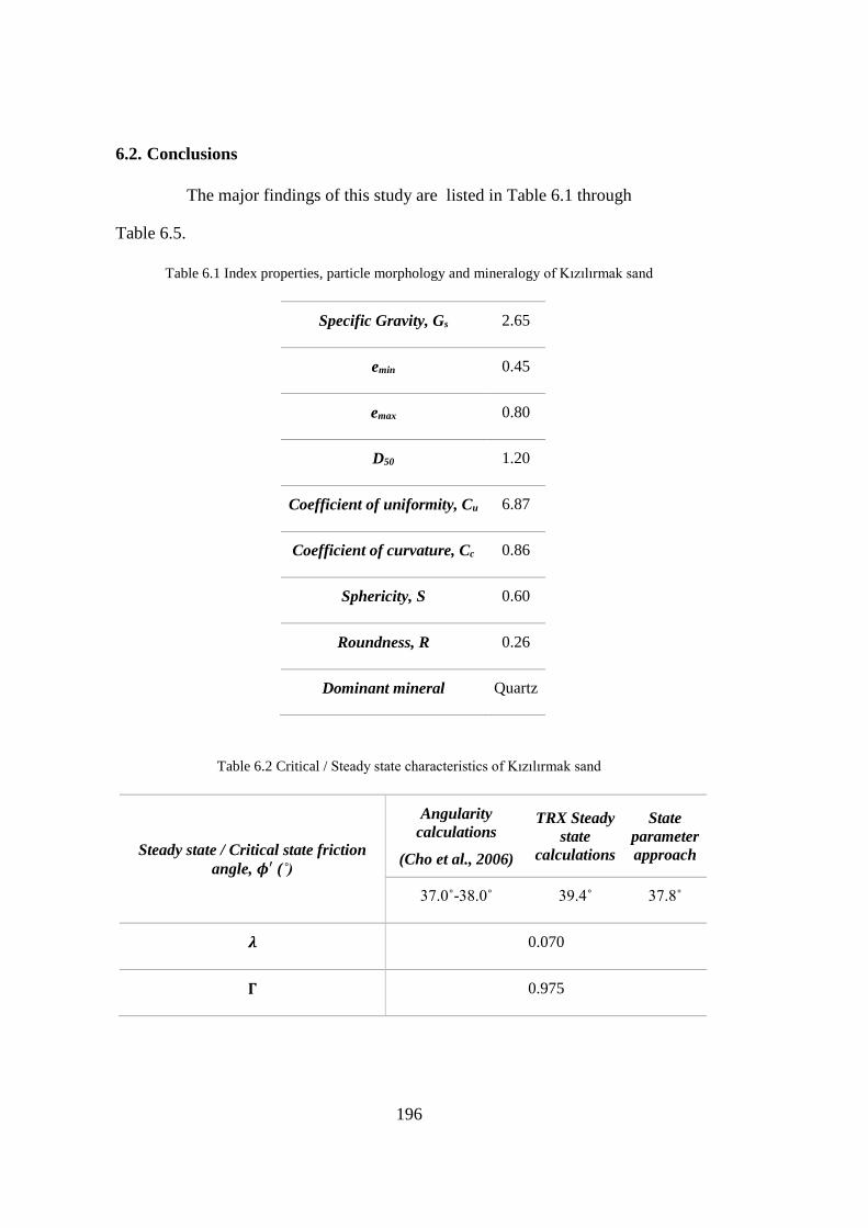
196

6.2. Conclusions

The major findings of this study are listed in Table 6.1 through

Table 6.5.

Table 6.1 Index properties, particle morphology and mineralogy of Kızılırmak sand

Specific Gravity, Gs 2.65

emin 0.45

emax 0.80

D50 1.20

Coefficient of uniformity, Cu 6.87

Coefficient of curvature, Cc 0.86

Sphericity, S 0.60

Roundness, R 0.26

Dominant mineral Quartz

Table 6.2 Critical / Steady state characteristics of Kızılırmak sand

Steady state / Critical state friction

angle, 𝝓′ (˚)

Angularity

calculations

(Cho et al., 2006)

TRX Steady

state

calculations

State

parameter

approach

37.0˚-38.0˚ 39.4˚ 37.8˚

𝝀 0.070

𝚪 0.975

197

Table 6.3 Mechanical properties of Kızılırmak sand

~35% RD

(N1,60≈5*)

~45% RD

(N1,60≈8*)

~60% RD

(N1,60≈15*)

~75% RD

(N1,60≈23*)

~80% RD

(N1,60≈26*)

Peak

friction

angle, 𝝓′ (˚)

36.5˚- 39.0˚ 36.0˚ - 40.0˚ 39.5˚ - 40.5˚ 40.5˚ - 42.5˚ 42.0˚ - 44.0˚

Yield stress,

𝝈𝒚′ (MPa)

~2.15 ~2.70 ~3.40 ~3.80 ~3.95

𝝈𝒗′ (𝑪𝑪,𝒎𝒂𝒙)

(MPa) ~8.1 ~14.6 ~14.6 ~14.6 ~14.6

𝑪𝑪,𝒎𝒂𝒙 ~0.190-

0.206 ~0.200 ~0.162 ~0.123

~0.111-

0.113

𝑪𝜶/𝑪𝑪 ~0.027-

0.030 ~0.031 ~0.032 ~0.035

~0.033-

0.037

* Normalized SPTN values to 𝜎𝑣′=100 kPa (Meyerhof, 1957)

Table 6.4 Triaxial modulus relationships proposed for linear elastic-perfectly plastic models

K n R2


′

𝑃𝑎)

𝑛

285 0.7 0.86


𝑃𝑎)

𝑛

323 0.6 0.44

𝐸𝑇𝑅𝑋 = [(2.17 − 𝑒0)2/(1 + 𝑒0)]𝐾𝑃𝑎 (𝜎3

′

𝑃𝑎)

𝑛

183 0.7 0.80

𝐸𝑇𝑅𝑋 = [𝑒−1.3]𝐾𝑃𝑎 (𝜎3

′

𝑃𝑎)

𝑛

143 0.7 0.78

𝐸𝑇𝑅𝑋 = [(2.17 − 𝑒𝑐)2/(1 + 𝑒𝑐)]𝐾𝑃𝑎 (𝑝′

𝑃𝑎)

𝑛

173 0.7 0.58

𝐸𝑇𝑅𝑋 = [𝑒−1.3]𝐾𝑃𝑎 (𝑝′

𝑃𝑎)

𝑛

134 0.7 0.55

198

Table 6.5 Duncan and Chang (1970) nonlinear elastic-perfectly plastic model's parameters

K 340

n 0.7

c* 0

𝝓′ (45.17 ∗ 𝑅𝐷0.224) − Δ𝜙 log10 (𝜎3

𝑝𝑎)

𝜟𝝓′(°) 1.5

Rf 0.7

*c=0 for clean sand

Due to the dilative nature of Kızılırmak sand under studied stress and density states,

perfectly plastic models are judged to be overly conservative to model post failure.

Hence, they are not recommended to assess the response of Kızılırmak sand in an

unbiased manner.

At low stress levels, the stiffness of Kızılırmak sand increases with increasing

confining stresses. After ~6.5-8.0 MPa vertical stress levels, stiffness stays constant

with increasing effective vertical stress. This constant stiffness range ended up at

~8.0-14.5 MPa stress levels. Then, the stiffness starts to increase with increasing

stresses. Therefore, Kızılırmak sand is classified as a soil, which exhibits Type B

volumetric straining response. As a reminder Type B volumetric straining illustration

is given in Figure 6.1.

Figure 6.1. Type B volumetric straining response (Mesri and Vardhanabhuti, 2009)

199

The gradation of Kızılırmak sand changes with increasing vertical stresses due to

particle crushing. Table 6.6 summarizes this change. As a reminder, note that the

first three rows in Table 6.6 simply designates the vertical shift in the particle size

gradation curves at 33.5 MPa. The last row, however presents the ratio of D15 before

and after testing.

Table 6.6 Grain size distribution shift after particle breakage

OED_25 OED_35 OED_45 OED_60 OED_75 OED_80 OED_85 average

Leslie, 1963 (%) 3.1 3.3 3.1 2.9 2.5 2.1 1.9 2.7

Leslie, 1975 (%) 4.3 5.9 5.9 8.3 5.3 5.1 1.4 5.2

Marsal, 1965 (%) 3.7 5.2 5.2 8.7 5.1 4.6 1.9 4.9

Lee and

Farhoomand,

1967 (-)

1.180 1.307 1.297 1.450 1.251 1.242 0.991 1.246

Similarly in Table 6.7, the shifts in grain size distributions are presented for the

sample with relative density 35 % and subjected to 4.5, 17.1 and 33.5 MPa vertical

stresses. This table also illustrates Kızılırmak sand becoming finer with increasing

vertical stresses and more pronounced particle crushing.

Table 6.7 Grain size distribution shift for the specimen prepared at 35% relative density and

subjected to vertical stresses of 4.5, 17.1 and 33.5 MPa

4.5 MPa 17.1 MPa 33.5 MPa

Leslie, 1963 (%) 0.1 1.3 3.3

Leslie, 1975 (%) 1.2 1.6 5.9

Marsal, 1965 (%) 1.3 1.3 5.2

Lee and Farhoomand, 1967 (-) 1.019 1.025 1.307

Figure 6.2 presents the increase in compression index with increasing effective

vertical stresses up to 8-14 MPa. Beyond these stresses, an increase in stiffness (also

a decrease in Cc values ) response is observed, which is consistent with similar sands

200

studied in the literature (Mesri and Vardhanabhuti, 2009). In Figure 6.2, the test

results for compression pressures less than 100 kPa were filtered out.


0.0001 0.001 0.01 0.1 1 10 100 1000 10000

Com

pre

ssio

n i

nd

ex,

Cc

0.001

0.01

0.1

1

10

Kızılırmak Sand

Dr=0%

50%

100%

Figure 6.2. Comparison of the compression index of Kızılırmak sand with Mesri and

Vardhanabhuti (2009) database

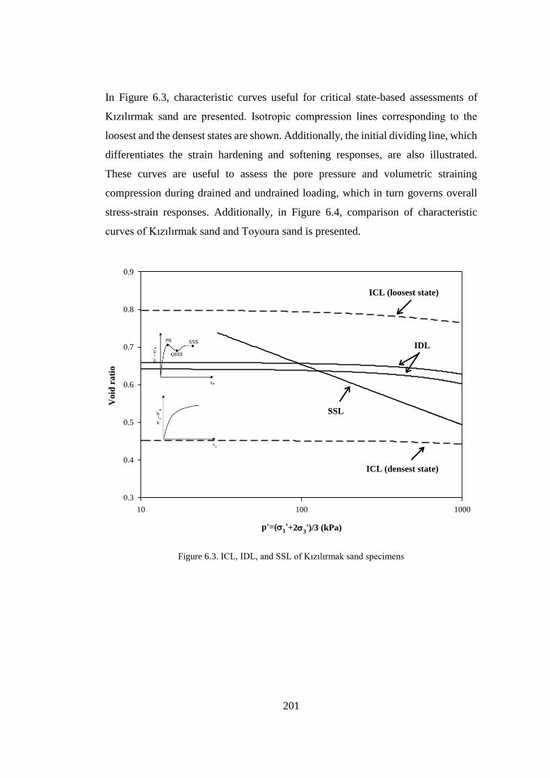
201

In Figure 6.3, characteristic curves useful for critical state-based assessments of

Kızılırmak sand are presented. Isotropic compression lines corresponding to the

loosest and the densest states are shown. Additionally, the initial dividing line, which

differentiates the strain hardening and softening responses, are also illustrated.

These curves are useful to assess the pore pressure and volumetric straining

compression during drained and undrained loading, which in turn governs overall

stress-strain responses. Additionally, in Figure 6.4, comparison of characteristic

curves of Kızılırmak sand and Toyoura sand is presented.

p'=(1'+2

3')/3 (kPa)

10 100 1000

Vo

id r

ati

o

0.3

0.4

0.5

0.6

0.7

0.8

0.9

ICL (loosest state)

IDL

ICL (densest state)

SSL

Figure 6.3. ICL, IDL, and SSL of Kızılırmak sand specimens

202

p'=(1'+2

3')/3 (kPa)

10 100 1000 10000

Void

rati

o

0.3

0.4

0.5

0.6

0.7

0.8

0.9

1.0

1.1

Kızılırmak sand

Toyoura sand

ICLIDL

ICL

SSL

ICL

IDL

SSL

QSSL

ICL

Figure 6.4. Comparison of characteristic curves of Kızlırmak sand and Toyoura sand

203

6.3. Future Works

In this study, the conclusions were listed based on consolidated undrained triaxial

and one-dimensional oedometer tests, which were loaded up to a maximum stress

level of ~33.5 MPa. Experiments with different failure modes and boundary

conditions, using simple shear or torsional shear apparatus, and compression or

extension loading schemes are recommended to be performed on Kızılırmak sand to

test the uniqueness of the parameters presented herein. Additionally, one-

dimensional compression tests may be repeated under higher stress levels.

Angularity calculations were performed in 2-D space. 3-D assessments may be

performed to improve the accuracy of results. Besides, a more detailed assessment

can be performed regarding the mineralogy of Kızılırmak sand.

Since Kızılırmak sand is angular, and shows dilative response, it hardens with shear

straining. Therefore, linear-elastic and nonlinear elastic perfectly plastic models are

not adequate to model Kızılırmak sand's post failure shearing behavior.

Alternatively, strain hardening/softening constitutive models can be considered for

an improved modeling of Kızılırmak sand's shearing response.

Last but not least, a Kızılırmak sand specific constitutive model, addressing particle

yielding at larger stress levels for the assessment of shear and volumetric straining

responses, are recommended to be developed.

205

REFERENCES

Alarcon-Guzman, A., Leonards, G. A. and Chameau, J. L. (1988) ‘Undrained

monotonic and cyclic strength of sands’, Journal of Geotechnical Engineering,

114(10). doi: 10.1061/(ASCE)0733-9410(1988)114:10(1089).

Alshibli, K. A. and Alsaleh, M. I. (2004) ‘Characterizing surface roughness and

shape of sands using digital microscopy’, Journal of Computing in Civil

Engineering, 18(1). doi: 10.1061/(ASCE)0887-3801(2004)18:1(36).

Alshibli, K. A. and Cil, M. B. (2018) ‘Influence of particle morphology on the

friction and dilatancy of sand’, Journal of Geotechnical and Geoenvironmental

Engineering, 144(3). doi: 10.1061/(ASCE)GT.1943-5606.0001841.

Altomare, A. et al. (2015) ‘QUALX2.0: A qualitative phase analysis software using

the freely available database POW-COD’, Journal of Applied Crystallography.

International Union of Crystallography, 48, pp. 598–603. doi:

10.1107/S1600576715002319.

Altuhafi, F. N. and Coop, M. R. (2011) ‘The effect of mode of loading on particle-

scale damage’, Soils and Foundations, 51(5). doi: 10.3208/sandf.51.849.

Andersen, K. H. and Schjetne, K. (2013) ‘Database of friction angles of sand and

consolidation characteristics of sand, silt, and clay’, Journal of Geotechnical and

Geoenvironmental Engineering, 139(7). doi: 10.1061/(ASCE)GT.1943-

5606.0000839.

ASTM International (2011a) ‘D2435/D2435M − 11 Standard one-dimensional

consolidation properties of soils using incremental loading’, ASTM Standards. doi:

10.1520/D2435.

ASTM International (2011b) ‘D4767−11 Standard test method for consolidated

undrained triaxial compression test for cohesive soils’, ASTM Standards. doi:

10.1520/D4767-11.2.

206

ASTM International (2014) ‘D854-14 Standard test methods for specific gravity of

soil solids by water pycnometer’, ASTM Standards. doi: 10.1520/D0854-10.2.

ASTM International (2016) ‘D4254−16 Standard test methods for minimum index

density and unit weight of soils and calculation of relative density’, ASTM Standards.

doi: https://doi.org/10.1520/D4253-16E01.

ASTM International (2017) ‘D6913-D6913M-17 Standard test methods for particle-

size distribution (gradation) of soils using sieve analysis’, ASTM Standards. doi:

10.1520/D6913-04R09.2.

Atkinson, J. (2007) The mechanics of soils and foundations. Available at:

https://books.google.com/books?hl=en&lr=&id=KRR34SOOUNAC&oi=fnd&pg=

PP1&dq=The+Mechanics+of+Soils+and+Foundations+atkinson&ots=y3KMX_JH

jB&sig=m5-QvqW6i8EZH--4lhO1YKA4YUI (Accessed: 5 September 2020).

Atkinson, J. H. (2000) ‘Non-linear soil stiffness in routine design’, Geotechnique,

50(5). doi: 10.1680/geot.2000.50.5.487.

Atkinson, J. H. and Sallfors, G. (1991) ‘Experimental determination of stress-strain-

time characteristics in laboratory and in situ tests’, in Proceedings of the

International Conference on Soil Mechanics and Foundation Engineering.

Baldi, G. et al. (1990) ‘Modulus of sands from CPT’s and DMT’s’, Proc. 12th

international conference on soil mechanics and foundation engineering, Rio de

Janeiro, 1989. Vol. 1. doi: 10.1016/0148-9062(91)93491-n.

Barden, L., Ismail, H. and Tong, P. (1969) ‘Plane strain deformation of granular

material at low and high pressures’, Geotechnique, 19(4). doi:

10.1680/geot.1969.19.4.441.

Been, K., Hachey, J. and Jefferies, M. G. (1991) ‘The critical state of sands’,

Geotechnique, 41(3). doi: 10.1680/geot.1991.41.3.365.

Been, K. and Jefferies, M. G. (1985) ‘A state parameter for sands’, Geotechnique,

35(2). doi: 10.1680/geot.1985.35.2.99.

207

De Beer, E. E. (1963) ‘The scale effect in the transposition of the results of deep-

sounding tests on the ultimate bearing capacity of piles and caisson foundations’,


Benz, T. (2007) ‘Small-strain stiffness of soils and its numerical consequences’.

Biarez, J. and Hicher, P. (1994) Elementary mechanics of soil behaviour: saturated

remoulded soils. Available at:

https://www.cabdirect.org/cabdirect/abstract/19951904796 (Accessed: 1 October

2020).

Bilge, H. (2005) ‘Volumetric and deviatoric strain behavior of cohesionless soils

under cyclic loading’.

Bishop, A. W. (1966) ‘The strength of soils as engineering materials’, Géotechnique,

16(2). doi: 10.1680/geot.1966.16.2.91.

Bishop, A. W. (1972) ‘Shear strength parameters for undisturbed and remolded soil

specimens’, in Roscoe Memorial Symp., pp. 3–58.

Bolton, M. D. (1986) ‘The strength and dilatancy of sands’, Geotechnique, 36(1).

doi: 10.1680/geot.1986.36.1.65.

Casagrande, A. (1963) ‘The determination of pre-consolidation load and it’s

practical significance’, in Proc. Int. Conf. Soil Mech. Found. Eng. Cambridge, Mass.

Available at: https://ci.nii.ac.jp/naid/10018165483/ (Accessed: 5 September 2020).

Castro, G. (1975) ‘Liquefaction and cyclic mobility of saturated sands’, ASCE J

Geotech Eng Div, 101(6).

Castro, G. and Poulos, S. J. (1977) ‘Factors affecting liquefaction and cyclic

mobility’, ASCE J Geotech Eng Div, 103(6).

208

Cho, G. C., Dodds, J. and Santamarina, J. C. (2006) ‘Particle shape effects on

packing density, stiffness, and strength: Natural and crushed sands’, Journal of

Geotechnical and Geoenvironmental Engineering, 132(5). doi:

10.1061/(ASCE)1090-0241(2006)132:5(591).

Chuhan, F. A. et al. (2002) ‘Porosity loss in sand by grain crushing - Experimental

evidence and relevance to reservoir quality’, Marine and Petroleum Geology, 19(1).

doi: 10.1016/S0264-8172(01)00049-6.

Chuhan, F. A. et al. (2003) ‘Experimental compression of loose sands: Relevance to

porosity reduction during burial in sedimentary basins’, Canadian Geotechnical

Journal, 40(5). doi: 10.1139/t03-050.

Coop, M. R. (1990) ‘The mechanics of uncemented carbonate sands’, Geotechnique,

40(4). doi: 10.1680/geot.1990.40.4.607.

Coop, M. R. (1993) ‘The behaviour of granular soils at elevated stresses’, Predictive

soil mechanics. Proc. of the Wroth memorial symposium, Oxford, 1992.

Cornforth, D. H. (1973) Prediction of Drained Strength of Sands from Relative

Density Measurements. Available at: www.astm.org (Accessed: 4 September 2020).

Cubrinovski, M. and Ishihara, K. (1998) ‘State concept and modified elastoplasticity

for sand modelling’, Soils and Foundations, 38(4). doi: 10.3208/sandf.38.4_213.

Cundall, P. A. and Strack, O. D. L. (1979) ‘A discrete numerical model for granular

assemblies’, Geotechnique, 29(1). doi: 10.1680/geot.1979.29.1.47.

Duncan, J. M. and Chang, C. Y. (1970) ‘Nonlinear analysis of stress and strain in

soils’, Journal of Soil Mechanics & Foundations Div.

Hagerty, M. M. et al. (1993) ‘One-dimensional high-pressure compression of

granular media’, Journal of Geotechnical Engineering, 119(1). doi:

10.1061/(ASCE)0733-9410(1993)119:1(1).

209

Hardin, B. O. (1985) ‘Crushing of soil particles’, Journal of Geotechnical

Engineering, 111(10). doi: 10.1061/(ASCE)0733-9410(1985)111:10(1177).

Hardin, B. O. and Black, W. L. (1969) ‘Closure to: Vibration modulus of normally

consolidated clays’, J. Journal of Soil Mechanics and Foundation Division, ASCE,

95(6). doi: 10.1186/s13287-017-0683-2.

Hardin, B. and Richart, F. (1963) ‘Elastic wave velocities in granular soils’, Journal

of the Soil Mechanics and Foundations Division, 89(1).

Houlsby, G. T. (1991) ‘How the dilatancy of soils affects their behaviour -done’,

International Proceedings of the 10th European Conference on Soil Mechanics and

Foundation Engineering.

Ishihara, K. (1993) ‘Liquefaction and flow failure during earthquakes’,


Ishihara, K. (1996) Soil behaviour in earthquake geotechnics. New York: Oxford

University Press Inc.

Janbu, N. (1963) ‘Soil compressibility as determined by odometer and triaxial tests’,

in Proc. Europ. Conf. SMFE, pp. 19–25.

Jefferies, M. and Been, K. (2006) Soil Liquefaction. Abingdon, UK: Taylor &

Francis. doi: 10.4324/9780203301968.

Kang, X. et al. (2019) ‘The critical state and steady state of sand: A literature review’,

Marine Georesources and Geotechnology, 37(9). doi:

10.1080/1064119X.2018.1534294.

Koener, R. (1968) ‘’The behavior of cohesionless materials formed from various

materials’.

Kondner, R. L. (1963) ‘A hyperbolic stress-strain formulation for sands’, in Proc. 2

nd Pan Am. Conf. on Soil Mech. and Found. Eng. Brazil, pp. 289–324.

210

Krumbein, W. C. and Sloss, L. L. (1963) Stratigraphy and sedimentation. San

Francisco: H Freeman and Company.

Kwag, J. M., Ochiai, H. and Yasufuku, N. (1999) ‘Yield stress characteristics of

carbonate sand in relation to individual particle fragmentation strength’, in

Engineering for Calcareous Sediments.

Ladd, R. S. (1978) ‘Preparing test specimens using undercompaction’, Geotechnical

Testing Journal, 1(1), pp. 16–23.

Lade, P. V. and Liu, C. T. (1998) ‘Experimental study of drained creep behavior of

sand’, Journal of Engineering Mechanics, 124(8). doi: 10.1061/(ASCE)0733-

9399(1998)124:8(912).

Lade, P. V. and Nelson, R. B. (1987) ‘Modelling the elastic behaviour of granular

materials’, International Journal for Numerical and Analytical Methods in

Geomechanics, 11(5). doi: 10.1002/nag.1610110507.

Lade, P. V., Yamamuro, J. A. and Bopp, P. A. (1996) ‘Significance of particle

crushing in granular materials’, Journal of Geotechnical Engineering, 122(4). doi:

10.1061/(asce)0733-9410(1996)122:4(309).

Lambe, T. W. and Whitman, R. V. (1969) Soil mechanics. New York: John Willey

& Sons. Inc.

Lee, K. L. and Farhoomand, I. (1967) ‘Compressibility and crushing of granular soil

in anisotropic triaxial compression’, Canadian Geotechnical Journal, 4(1). doi:

10.1139/t67-012.

Leslie, D. D. (1963) ‘Large scale triaxial tests on gravelly soils’, in Proceedings of

the 2nd Panamerican Conference on Soil Mechanics and Foundation Engineering.

Brazil, pp. 181–202.

Leslie, D. D. (1975) Shear strength of rockfill. California.

211

Mair, R. J. (1993) ‘Developments in geotechnical engineering research: application

to tunnels and deep excavations’, in Proceedings of Institution of Civil Engineers:

Civil Engineering, pp. 27–41.

Marsal, R. J. (1965) ‘Discussion of Shear Strength’, in Proceedings of the 6th

International Conference on Soil Mechanics and Foundaiton Engineering.

Montreal, pp. 310–316.

Marsal, R. J. (1967) ‘Large scale testing of rockfill materials’, Journal of Soil

Mechanics and Foundations Division, ASCE, 93(SM2).

McDowell, G. R. and Bolton, M. D. (1998) ‘On the micromechanics of crushable

aggregates’, Geotechnique, 48(5). doi: 10.1680/geot.1998.48.5.667.

McDowell, G. R., Bolton, M. D. and Robertson, D. (1996) ‘The fractal crushing of

granular materials’, Journal of the Mechanics and Physics of Solids, 44(12). doi:

10.1016/S0022-5096(96)00058-0.

McDowell, G. R. and Harireche, O. (2002) ‘Discrete element modelling of yielding

and normal compression of sand’, Geotechnique, 52(4). doi:

10.1680/geot.2002.52.4.299.

Mesri, G. et al. (1981) ‘Shear stress-strain-time behaviour of clays’, Géotechnique.

Thomas Telford Ltd , 31(4), pp. 537–552. doi: 10.1680/geot.1981.31.4.537.

Mesri, G. and Vardhanabhuti, B. (2009) ‘Compression of granular materials’,

Canadian Geotechnical Journal, 46(4). doi: 10.1139/T08-123.

Meyerhof, G. G. (1957) ‘Discussion on research on determining the density of sands

by penetration testing’, in Proc. 4th Int. Conf. on Soil Mech. And Found. Engrg.

Miao, G. and Airey, D. (2013) ‘Breakage and ultimate states for a carbonate sand’,

Geotechnique, 63(14). doi: 10.1680/geot.12.P.111.

212

Murayama, S. (1983) ‘Formulation of stress-strain-time behavior of soils under

deviatoric stress condition’, Soils and Foundations, 23(2). doi:

10.3208/sandf1972.23.2_43.

Murayama, S., Michihiro, K. and Sakagami, T. (1984) ‘Creep characteristics of

sands’, Soils and Foundations, 24(2). doi: 10.3208/sandf1972.24.2_1.

Nakata, Y., Hyodo, M., et al. (2001) ‘Microscopic particle crushing of sand

subjected to high pressure one-dimensional compression’, Soils and Foundations,

41(1). doi: 10.3208/sandf.41.69.

Nakata, Y., Kato, Y., et al. (2001) ‘One-dimensional compression behaviour of

uniformly graded sand related to single particle crushing strength’, Soils and

Foundations, 41(2). doi: 10.3208/sandf.41.2_39.

Pestana, J. M. and Whittle, A. J. (1995) ‘Compression model for cohesionless soils’,


Poulos, S. J. (1981) ‘The steady state of deformation.’, Journal of the Geotechnical

Engineering Division, ASCE, 107(GT5, Proc. Paper, 16241).

Rahim, A. (1989) ‘Effect of morphology and mineralogy on compressibility of

sands’.

Roberts, J. (1965) ‘Sand compression as a factor in oil field subsidence.’ Available

at: https://dspace.mit.edu/bitstream/handle/1721.1/13626/24228445-

MIT.pdf?sequence=2 (Accessed: 5 September 2020).

Roberts, J. E. and de Souza, J. M. (1958) ‘The compressibility of sands’, Proceedings

of the American Society of Testing and Materials, 58.

Roscoe, K. H., Schofield, A. N. and Wroth, C. P. (1958) ‘On the yielding of soils’,


213

Rowe, P. W. (1962) ‘The stress-dilatancy relation for static equilibrium of an

assembly of particles in contact’, Proceedings of the Royal Society of London. Series

A. Mathematical and Physical Sciences, 269(1339). doi: 10.1098/rspa.1962.0193.

Schofield, A. and Wroth, P. (1968) Critical state soil mechanics, Engineer.

Stroud, M. (1971) ‘The behaviour of sand at low stress levels in the simple-shear

apparatus’. Available at: https://www.repository.cam.ac.uk/handle/1810/265294

(Accessed: 4 September 2020).

Takei, M., Kusakabe, O. and Hayashi, T. (2001) ‘Time-dependent behavior of

crushable materials in one-dimensional compression tests’, Soils and Foundations,

41(1). doi: 10.3208/sandf.41.97.

Tatar, H. M. (2018) Consolidated undrained shearing response of hydrophobic

sands.

Taylor, D. (1948) Fundamentals of soil mechanics. Available at:

https://journals.lww.com/soilsci/Citation/1948/08000/Fundamentals_of_Soil_Mech

anics.8.aspx (Accessed: 4 September 2020).

Vaid, Y. P., Chern, J. C. and Tumi, H. (1985) ‘Confining pressure, grain angularity,

and liquefaction’, Journal of Geotechnical Engineering, 111(10). doi:

10.1061/(ASCE)0733-9410(1985)111:10(1229).

Vaid, Y. P., Chung, E. K. F. and Kuerbis, R. H. (1990) ‘Stress path and steady state’,

Canadian Geotechnical Journal, 27(1). doi: 10.1139/t90-001.

Vesic, A. S. and Clough, G. W. (1968) ‘Behavior of granular materials under high

stresses’, Journal of Terramechanics, 5(3). doi: 10.1016/0022-4898(68)90104-3.

Wong, K. S. and Duncan, J. M. (1974) Hyperbolic stress-strain parameters for

nonlinear finite element analyses of stresses and movements in soil masses.

214

Wroth, C. P. and Houlsby, G. T. (1985) ‘Soil mechanics - property characterization

and analysis procedures.’, Proc. 11th international conference on soil mechanics and

foundation engineering, San Francisco, August 1985. Vol. 1, (Balkema).

Wu, Y., Yamamoto, H. and Izumi, A. (2016) ‘Experimental investigation on

crushing of granular material in one-dimensional test’, Periodica Polytechnica Civil

Engineering, 60(1). doi: 10.3311/PPci.8028.

Yudhbir and Rahim, A. (1987) ‘Compressibility characteristics of sands’, in

Proceedings of the 9th Southeast Asian Geotechnical Conference, pp. 483–494.

215

APPENDICES

A. Appendix A

Table A-1: Details of specific gravity tests

Experiment No. 1 2

Temperature (C) 20.6 23.1

Trial No. 1 2 1 2

Mass of empty bottle, 𝑀𝑏 (g) 125.552 122.737 122.803 115.089

Mass of bottle filled with water only,

𝑀𝑏+𝑤 (g) 386.002 390.628 390.427 377.542

Mass of bottle with dry soil, 𝑀𝑏+𝑠 (g) 165.53 162.713 185.684 175.568

Mass of solids, 𝑀𝑏+𝑠 − 𝑀𝑏 (= 𝑀𝑠) (g) 39.978 39.976 62.881 60.479

Mass of bottle with soil, filled with

deaired water, 𝑀𝑏+𝑠+𝑤 (g) 410.923 415.499 429.665 415.15

Mass of water with volume equal to the

volume of solids, 𝑀𝑏+𝑤 + 𝑀𝑠 −

𝑀𝑏+𝑠+𝑤 (g)

15.057 15.105 23.643 22.871

Specific gravity of solids at this

temperature, 𝐺𝑠 2.655 2.647 2.660 2.644

Specific gravity of solids at 20°C,

𝐺𝑠@20°𝐶 2.655 2.646 2.653 2.638

Mean value of Gs 2.650 2.645

Standard Deviation 0.006 0.011

216

B. Appendix B

Table B-1: Details of maximum void ratio calculations

Experiment No. 1 2 3

Diameter of mold (mm) 152.01 152.01 152.01

Height of mold (mm) 116.57 116.57 116.57

Volume of mould (cm3) 2114.62 2114.62 2114.62

Mass of mold (g) 5544.7 5544.7 5544.7

Specific gravity of soil 2.65 2.65 2.65

Mass of Soil + Mould (g) 8675.2 8640.1 8664

Mass of Soil (g) 3130.5 3095.4 3119.3

Volume of Soil Particles ( cm3) 1181.321 1168.075 1177.094

Volume of Voids (cm3) 933.299 946.544 937.525

Maximum void ratio 0.790 0.810 0.796

217

Table B-2: Details of minimum void ratio calculations

Experiment No. 1 2

Diameter of the mold (mm) 152.05 152.01

Height of the mold (mm) 116.51 116.51

Volume of the mould (cm3) 2114.583 2113.471

Mass of the mold (g) 5563.6 5545.2

Specific gravity of the soil samples 2.65 2.65

Mass of Soil + Mould (g) 9391.1 9428.2

Mass of Soil (g) 3827.5 3883

Volume of Soil Particles ( cm3) 1444.34 1465.283

Volume of Voids (cm3) 670.243 648.188

Maximum void ratio 0.464 0.442

Documents

SHEARING AND VOLUMETRIC STRAINING RESPONSE OF …