Embed Size (px)
Citation preview

Sheet feedback control design in a printer paper path
Bukkems, B.H.M.
DOI:10.6100/IR625902
Published: 01/01/2007
Document VersionPublisher’s PDF, also known as Version of Record (includes final page, issue and volume numbers)
Please check the document version of this publication:
• A submitted manuscript is the author's version of the article upon submission and before peer-review. There can be important differencesbetween the submitted version and the official published version of record. People interested in the research are advised to contact theauthor for the final version of the publication, or visit the DOI to the publisher's website.• The final author version and the galley proof are versions of the publication after peer review.• The final published version features the final layout of the paper including the volume, issue and page numbers.
Link to publication
Citation for published version (APA):Bukkems, B. H. M. (2007). Sheet feedback control design in a printer paper path Eindhoven: TechnischeUniversiteit Eindhoven DOI: 10.6100/IR625902
General rightsCopyright and moral rights for the publications made accessible in the public portal are retained by the authors and/or other copyright ownersand it is a condition of accessing publications that users recognise and abide by the legal requirements associated with these rights.
• Users may download and print one copy of any publication from the public portal for the purpose of private study or research. • You may not further distribute the material or use it for any profit-making activity or commercial gain • You may freely distribute the URL identifying the publication in the public portal ?
Take down policyIf you believe that this document breaches copyright please contact us providing details, and we will remove access to the work immediatelyand investigate your claim.
Download date: 07. Sep. 2018

Sheet Feedback Control Designin a Printer Paper Path

This PhD-study has been carried out as part of the Boderc project under the responsibility of theEmbedded Systems Institute. This project is partially supported by the Netherlands Ministry ofEconomic Affairs under the Senter TS program.
A catalogue record is available from the Library Eindhoven University of Technology
Bukkems, Björn H.M.
Sheet Feedback Control Design in a Printer Paper Path / by Björn H.M. Bukkems. –Eindhoven : Technische Universiteit Eindhoven, 2007.Proefschrift. – ISBN-13: 978-90-386-0974-4NUR 978Trefwoorden: document doorvoer systemen / terugkoppelingsgebaseerde regelingvan de velloop / hiërarchisch regelen / stuksgewijs lineaire systemen /robuust regelen / lineaire matrix ongelijkheden / experimentele validatieSubject headings: document handling systems / sheet feedback control /hierarchical control / piecewise linear systems / robust control /linear matrix inequalities / experimental validation
Copyright c© 2007 by B.H.M. Bukkems.
All rights reserved. This publication may not be translated or copied, in whole or inpart, or used in connection with any form of information storage and retrieval,electronic adaptation, electronic or mechanical recording, including photocopying orby any similar or dissimilar methodology now known or developed hereafter, withoutthe written permission of the copyright holder.
This thesis was prepared with the LATEX2ε documentation system.Cover Design: Oranje Vormgevers, Eindhoven, The Netherlands.Reproduction: Universiteitsdrukkerij TU Eindhoven, Eindhoven, The Netherlands.
Sheet Feedback Control Designin a Printer Paper Path
PROEFSCHRIFT
ter verkrijging van de graad van doctoraan de Technische Universiteit Eindhoven,
op gezag van de Rector Magnificus, prof.dr.ir. C.J. van Duijn,voor een commissie aangewezen door het College voor Promoties
in het openbaar te verdedigenop dinsdag 5 juni 2007 om 16.00 uur
door
Björn Hubertus Maria Bukkems
geboren te Geldrop

Dit proefschrift is goedgekeurd door de promotor:
prof.dr.ir. M. Steinbuch
Copromotor:dr.ir. M.J.G. van de Molengraft
Contents
1 Introduction 1
1.1 The Boderc Research Project . . . . . . . . . . . . . . . . . . . . . . . . . 11.2 Sheet Handling in a Printer Paper Path . . . . . . . . . . . . . . . . . . . 41.3 Sheet Flow Modeling and Control . . . . . . . . . . . . . . . . . . . . . . . 61.4 Contribution of the Thesis . . . . . . . . . . . . . . . . . . . . . . . . . . . 91.5 Outline of the Thesis . . . . . . . . . . . . . . . . . . . . . . . . . . . . . . 11
2 The Sheet Feedback Control Architecture 13
2.1 Basic Paper Path Setup . . . . . . . . . . . . . . . . . . . . . . . . . . . . . 132.2 Paper Path and Sheet Flow Modeling . . . . . . . . . . . . . . . . . . . . . 142.3 Decomposition of the Sheet Handling Control Problem . . . . . . . . . . 17
3 State Feedback Control Design 23
3.1 The Tracking Control Problem . . . . . . . . . . . . . . . . . . . . . . . . 233.2 Nominal Sheet Feedback Control Design . . . . . . . . . . . . . . . . . . . 26
3.2.1 Controller Synthesis . . . . . . . . . . . . . . . . . . . . . . . . . . 263.2.1.1 Linearizing Controller Synthesis . . . . . . . . . . . . . . 313.2.1.2 Partially linearizing Controller Synthesis . . . . . . . . . 32
3.2.2 Control Design Results . . . . . . . . . . . . . . . . . . . . . . . . 333.2.2.1 Linearizing Feedback Control Design Results . . . . . . 343.2.2.2 Partially Linearizing Feedback Control Design Results . . 35
3.2.3 Simulation Results . . . . . . . . . . . . . . . . . . . . . . . . . . . 363.2.3.1 Linearizing Feedback Controller Results . . . . . . . . . 373.2.3.2 Partially Linearizing Feedback Controller Results . . . . 38
3.3 Analysis of the Perturbation of Paper Path Parameters . . . . . . . . . . . 413.3.1 Influence of Parameter Perturbations . . . . . . . . . . . . . . . . 433.3.2 Simulation Results . . . . . . . . . . . . . . . . . . . . . . . . . . . 46
3.4 Evaluation . . . . . . . . . . . . . . . . . . . . . . . . . . . . . . . . . . . . 51
v
vi CONTENTS
4 Output Feedback Control Design 53
4.1 The Tracking Control Problem . . . . . . . . . . . . . . . . . . . . . . . . 534.2 Nominal Sheet Feedback Control Design . . . . . . . . . . . . . . . . . . . 55
4.2.1 Controller Synthesis . . . . . . . . . . . . . . . . . . . . . . . . . . 554.2.2 Control Design Results . . . . . . . . . . . . . . . . . . . . . . . . 604.2.3 Simulation Results . . . . . . . . . . . . . . . . . . . . . . . . . . . 64
4.3 Robust Sheet Feedback Control Design . . . . . . . . . . . . . . . . . . . . 664.3.1 Uncertainty Modeling . . . . . . . . . . . . . . . . . . . . . . . . . 664.3.2 Controller Synthesis . . . . . . . . . . . . . . . . . . . . . . . . . . 684.3.3 Control Design Results . . . . . . . . . . . . . . . . . . . . . . . . 724.3.4 Simulation Results . . . . . . . . . . . . . . . . . . . . . . . . . . . 76
4.4 Stability Analysis for Non-ideal Low Level Dynamics . . . . . . . . . . . . 774.5 Evaluation . . . . . . . . . . . . . . . . . . . . . . . . . . . . . . . . . . . . 78
5 The Experimental Paper Path Setup 81
5.1 The Sheet Transportation Unit . . . . . . . . . . . . . . . . . . . . . . . . 815.2 Sheet Position Measurement . . . . . . . . . . . . . . . . . . . . . . . . . 83
5.2.1 Sensor Selection . . . . . . . . . . . . . . . . . . . . . . . . . . . . 835.2.2 Implementation . . . . . . . . . . . . . . . . . . . . . . . . . . . . 84
5.2.2.1 Calibration . . . . . . . . . . . . . . . . . . . . . . . . . 855.2.2.2 Sheet Position Measurement . . . . . . . . . . . . . . . . 86
6 Experimental Results 89
6.1 Low Level Motor Dynamics . . . . . . . . . . . . . . . . . . . . . . . . . . 896.2 Experimental Validation Results - The State Feedback Control Approach . 936.3 Experimental Validation Results - The Output Feedback Control Approach 100
6.3.1 Stability Analysis in Case of Non-ideal Low Level Dynamics . . . . 1006.3.2 Robustness Experiments . . . . . . . . . . . . . . . . . . . . . . . 101
7 Extensions of Sheet Feedback Control to Real Printer Paper Paths 107
7.1 Challenges in Industrial Paper Paths . . . . . . . . . . . . . . . . . . . . . 1077.2 Duplex Loop Modeling and Control . . . . . . . . . . . . . . . . . . . . . . 108
7.2.1 The Tracking Control Problem . . . . . . . . . . . . . . . . . . . . 1087.2.2 Sheet Feedback Control Design . . . . . . . . . . . . . . . . . . . . 1117.2.3 Simulation Results . . . . . . . . . . . . . . . . . . . . . . . . . . . 112
7.3 Sheet Transport via Multiple Pinches . . . . . . . . . . . . . . . . . . . . . 1137.3.1 The Tracking Control Problem . . . . . . . . . . . . . . . . . . . . 1137.3.2 High Level Sheet Flow Modeling and Control Design . . . . . . . . 1167.3.3 Low Level Motor Control Design . . . . . . . . . . . . . . . . . . . 117
7.3.3.1 Feedforward Control Structure . . . . . . . . . . . . . . . 1187.3.3.2 Feedforward Control Design Results . . . . . . . . . . . 120
CONTENTS vii
7.3.3.3 Feedback Control Design Results . . . . . . . . . . . . . 1217.3.4 Validation Results . . . . . . . . . . . . . . . . . . . . . . . . . . . 123
7.4 Coupling Pinches into Sections . . . . . . . . . . . . . . . . . . . . . . . . 1287.5 Evaluation . . . . . . . . . . . . . . . . . . . . . . . . . . . . . . . . . . . . 130
8 Conclusions and Recommendations 133
8.1 Conclusions . . . . . . . . . . . . . . . . . . . . . . . . . . . . . . . . . . 1338.2 Recommendations . . . . . . . . . . . . . . . . . . . . . . . . . . . . . . . 135
8.2.1 Recommendations for the Control Design Approaches . . . . . . . 1368.2.2 Recommendations for Integration and Implementation . . . . . . 137
A Linearizing Change of Variables 139
Bibliography 141
Summary 149
Samenvatting 151
Dankwoord 155
Curriculum Vitae 157

viii
CHAPTER ONE
Introduction
1.1 The Boderc Research Project . . . . . . . . . . . . . . . . . . . . . . . . 1
1.2 Sheet Handling in a Printer Paper Path . . . . . . . . . . . . . . . . . . 4
1.3 Sheet Flow Modeling and Control . . . . . . . . . . . . . . . . . . . . . . 6
1.4 Contribution of the Thesis . . . . . . . . . . . . . . . . . . . . . . . . . . 9
1.5 Outline of the Thesis . . . . . . . . . . . . . . . . . . . . . . . . . . . . . 11
1.1 The Boderc Research Project
A general trend in the design of high-tech systems as, for example, wafer steppers, elec-tron microscopes, and document handling systems, is the increasing number of require-ments imposed by its users. More functionality is asked for, while already existing func-tional properties must be preserved or, even more likely, improved. On the other hand,industrial constraints are becoming tighter. Product design cycles must be shortened anddevelopment costsmust be decreased to keep a competitive position in themarket. A con-sequence of this trend is an increasing complexity of the overall system design, which hasto be realized in less time and in close co-operation by multiple monodisciplinary engi-neering disciplines, such asmechanical, electrical, software, and control engineering [36].In each of these disciplines, the increasing system complexity results in an increase of thenumber of design decisions to be made. Erroneous decisions, especially the ones madein early design phases, can have a significant impact during product integration phases,as many other decisions will be based on them. Corrections in later project phases aredifficult to make and can therefore lead to a longer development period than planned orcan lead to a less optimal product [58].
1
2 1 INTRODUCTION
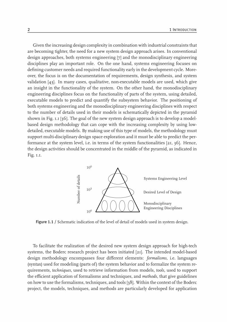
Given the increasing design complexity in combination with industrial constraints thatare becoming tighter, the need for a new system design approach arises. In conventionaldesign approaches, both systems engineering [7] and the monodisciplinary engineeringdisciplines play an important role. On the one hand, systems engineering focuses ondefining customer needs and required functionality early in the development cycle. More-over, the focus is on the documentation of requirements, design synthesis, and systemvalidation [43]. In many cases, qualitative, non-executable models are used, which givean insight in the functionality of the system. On the other hand, the monodisciplinaryengineering disciplines focus on the functionality of parts of the system, using detailed,executable models to predict and quantify the subsystem behavior. The positioning ofboth systems engineering and the monodisciplinary engineering disciplines with respectto the number of details used in their models is schematically depicted in the pyramidshown in Fig. 1.1 [36]. The goal of the new system design approach is to develop a model-based design methodology that can cope with the increasing complexity by using low-detailed, executable models. By making use of this type of models, the methodology mustsupport multi-disciplinary design space exploration and it must be able to predict the per-formance at the system level, i.e. in terms of the system functionalities [21, 36]. Hence,the design activities should be concentrated in the middle of the pyramid, as indicated inFig. 1.1.
Numberof
details
100
103
106
Systems Engineering Level
MonodisciplinaryEngineering Disciplines
Desired Level of Design
Figure 1.1 / Schematic indication of the level of detail of models used in system design.
To facilitate the realization of the desired new system design approach for high-techsystems, the Boderc research project has been initiated [21]. The intended model-baseddesign methodology encompasses four different elements: formalisms, i.e. languages(syntax) used for modeling (parts of) the system behavior and to formalize the system re-quirements, techniques, used to retrieve information from models, tools, used to supportthe efficient application of formalisms and techniques, and methods, that give guidelineson how to use the formalisms, techniques, and tools [38]. Within the context of the Bodercproject, the models, techniques, and methods are particularly developed for application
1.1 THE BODERC RESEARCH PROJECT 3
in the early design phases and must satisfy industrial application constraints. Moreover,they should enable fast design cycles to quickly yield insight in the influence of chang-ing design choices on the system performance. To facilitate this, a systematic design isrequired, which, among others, can be realized by deriving low-detailed, yet adequate,models that are capable of making predictions at the system level.
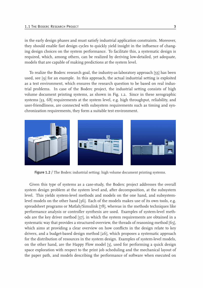
To realize the Boderc research goal, the industry-as-laboratory approach [55] has beenused, see [9] for an example. In this approach, the actual industrial setting is exploitedas a test environment, which ensures the research question to be based on real indus-trial problems. In case of the Boderc project, the industrial setting consists of highvolume document printing systems, as shown in Fig. 1.2. Since in these xerographicsystems [33, 68] requirements at the system level, e.g. high throughput, reliability, anduser-friendliness, are connected with subsystem requirements such as timing and syn-chronization requirements, they form a suitable test environment.
Figure 1.2 / The Boderc industrial setting: high volume document printing systems.
Given this type of systems as a case-study, the Boderc project addresses the overallsystem design problem at the system level and, after decomposition, at the subsystemlevel. This yields system-level methods and models on the one hand, and subsystem-level models on the other hand [36]. Each of the models makes use of its own tools, e.g.spreadsheet programs or Matlab/Simulink [78], whereas in the methods techniques likeperformance analysis or controller synthesis are used. Examples of system-level meth-ods are the key driver method [37], in which the system requirements are obtained in asystematic way that provides a structured overview, the threads of reasoning method [65],which aims at providing a clear overview on how conflicts in the design relate to keydrivers, and a budget-based design method [26], which proposes a systematic approachfor the distribution of resources in the system design. Examples of system-level models,on the other hand, are the Happy Flow model [3], used for performing a quick designspace exploration with respect to the print job scheduling and the mechanical layout ofthe paper path, and models describing the performance of software when executed on
4 1 INTRODUCTION
real platforms [81]. Zooming in at the subsystem level, examples of topics addressed inthe Boderc project are event-driven control [64, 66], the effect of time delay in networkedcontrol systems [16], and analysis techniques for real-time properties of software [24].Within the context of the project, one of the central questions is in which way controlengineering can contribute to the realization of the Boderc research goal. In response tothis question, this thesis takes as a case-study the design of a sheet handling system inthe paper path of document printing systems, since the paper path is a significant unitof the complete printing system in which motion control plays an important part. In thenext section, sheet handling in a printer paper path will be discussed in more detail.
1.2 Sheet Handling in a Printer Paper Path
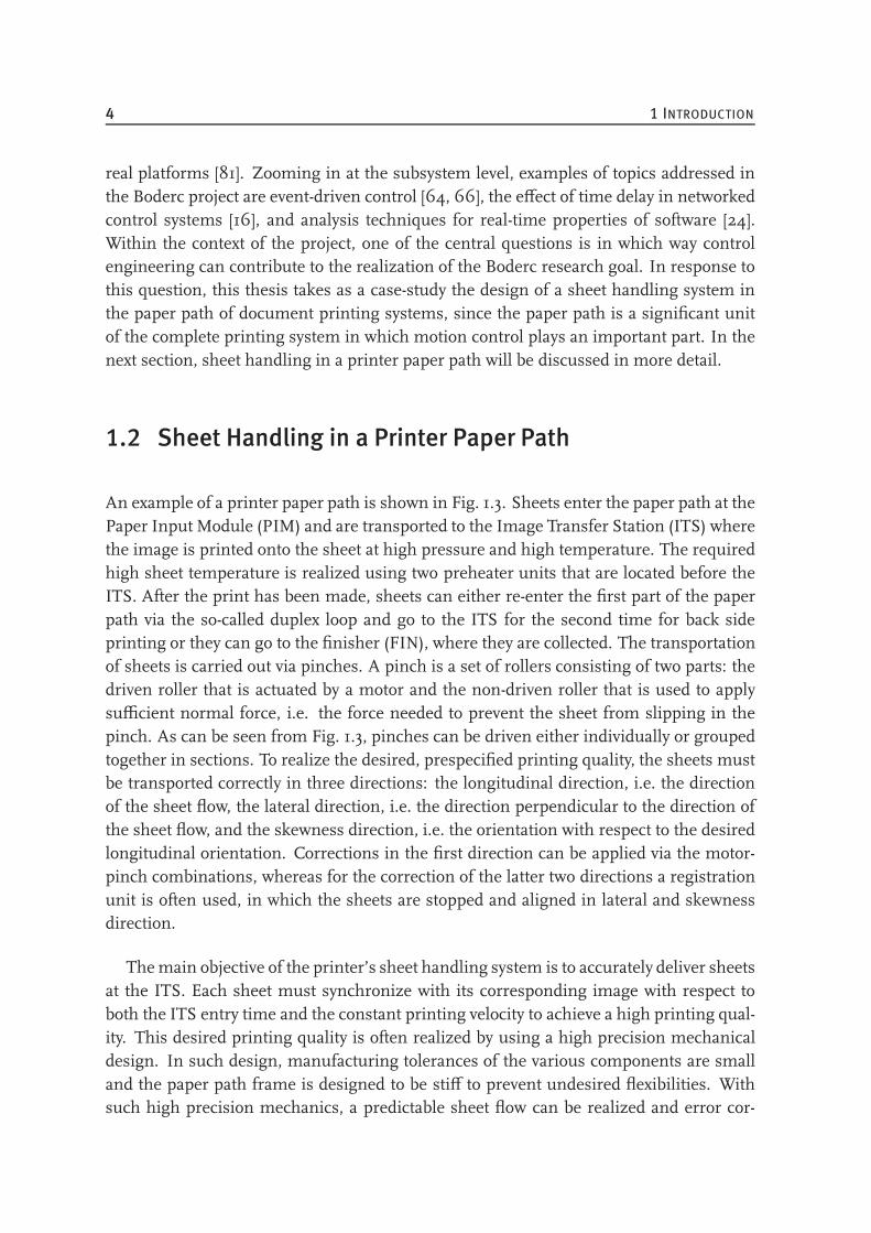
An example of a printer paper path is shown in Fig. 1.3. Sheets enter the paper path at thePaper Input Module (PIM) and are transported to the Image Transfer Station (ITS) wherethe image is printed onto the sheet at high pressure and high temperature. The requiredhigh sheet temperature is realized using two preheater units that are located before theITS. After the print has been made, sheets can either re-enter the first part of the paperpath via the so-called duplex loop and go to the ITS for the second time for back sideprinting or they can go to the finisher (FIN), where they are collected. The transportationof sheets is carried out via pinches. A pinch is a set of rollers consisting of two parts: thedriven roller that is actuated by a motor and the non-driven roller that is used to applysufficient normal force, i.e. the force needed to prevent the sheet from slipping in thepinch. As can be seen from Fig. 1.3, pinches can be driven either individually or groupedtogether in sections. To realize the desired, prespecified printing quality, the sheets mustbe transported correctly in three directions: the longitudinal direction, i.e. the directionof the sheet flow, the lateral direction, i.e. the direction perpendicular to the direction ofthe sheet flow, and the skewness direction, i.e. the orientation with respect to the desiredlongitudinal orientation. Corrections in the first direction can be applied via the motor-pinch combinations, whereas for the correction of the latter two directions a registrationunit is often used, in which the sheets are stopped and aligned in lateral and skewnessdirection.
Themain objective of the printer’s sheet handling system is to accurately deliver sheetsat the ITS. Each sheet must synchronize with its corresponding image with respect toboth the ITS entry time and the constant printing velocity to achieve a high printing qual-ity. This desired printing quality is often realized by using a high precision mechanicaldesign. In such design, manufacturing tolerances of the various components are smalland the paper path frame is designed to be stiff to prevent undesired flexibilities. Withsuch high precision mechanics, a predictable sheet flow can be realized and error cor-
1.2 SHEET HANDLING IN A PRINTER PAPER PATH 5
FUSE
FIN
PIM
ITS
Image
PinchMotorSheet sensorPreheater unit
Figure 1.3 / Schematic representation of a printer paper path.
rection during the sheet transport can be done at a few fixed locations in the paper pathonly. At these locations optical I/O sheet sensors, indicated in Fig. 1.3, are mounted thatcan detect the presence of a sheet. Based on this sheet detection, the sheet referencemotion profile can be slightly adjusted such that the sheet will meet its correspondingimage in the ITS right on time. A drawback of this approach is the fact that the design ofthe discrete-event sheet controllers is not carried out systematically; for each new printerto be designed, it takes much effort to determine where and how feedback needs to beapplied. Hence, fast design cycles in an early stage of the design are difficult to realize.
To improve the design trajectory of a sheet handling system, this thesis investigateshow control engineering can contribute to the optimization of the design trajectory ofsuch system. More specifically, having the Boderc research goal in mind, the questionis if a model-based methodology for the design of such sheet handling system can beformulated from a control engineering point of view. In order to find an answer to thisquestion, the goal of this thesis is to find a systematic approach for controlling the sheetflow, which is based on low-detailed, yet adequatemodels of the sheet flow and paper pathdynamics. Suchmodels should be both accurate enough tomake useful predictions of thephysical process and abstract enough to enable relevant reasoning with appropriate time-efficiency [4]. The approach to be designed should encompass three main characteristics.First of all, it should be applicable in early stages of the design process. Secondly, it shouldbe generic such that it can be used in various printer design projects, and thirdly, it shouldallow for fast design cycles such that insight in the effect of certain design decisions canbe quickly obtained. Hence, applying the approach for designing a sheet handling systemin an industrial design process should result in both a decrease of the development timeand an increase of the predictability of the design process.
6 1 INTRODUCTION
1.3 Sheet Flow Modeling and Control
To realize the intended design of a sheet handling system, models of the sheet flow andpaper path dynamics are needed. However, as we are dealing with a very specific applica-tion field, the amount of literature on paper path modeling is not too extensive. Yet, [32]and [31] present a compositional model of sheet transportation in a printer paper path.The model is meant for simulation and diagnosis, and is applicable to a variety of config-urations. The models presented cannot be directly used for model-based sheet controllersynthesis, but the key feature linking to the work presented in this thesis is the level ofabstraction used in the modeling. More specifically, the model presented in [32] abstractsaway from the physical forces and reasons only about velocities. Nonetheless, it succeedsin determining essential features of the motion of the sheet of paper like buckling andtearing.
Similar to paper path modeling, (model-based) control design for sheet handling sys-tems of document printing systems has not received widespread attention in the controlliterature either [33]. One of the first contributions that is considered relevant for thework described in this thesis, is presented in [56]. A hybrid hierarchical control archi-tecture for the transportation of sheets in a paper path is discussed. The transition fromthe open-loop operation of sheet handling mechanisms to the introduction of sheet feed-back control is discussed. A hybrid hierarchical control system architecture is proposed,in which a central supervisory controller plans overall trajectories for each sheet of pa-per. These trajectories are communicated to the low-level systems, i.e. to the motor-pinchcombinations that track the trajectories and provide an estimate of themotion of the sheetto the central controller. Based on this estimation, a new sheet trajectory can be plannedwhen collisions become likely to occur.
Elaborating on the results presented in [56], the work presented in [12, 46] discusses inmore detail the use of closed-loop longitudinal motion control of sheets in a printer paperpath. Motivated by the increasing demands on sheet handling capabilities, i.e. sheets witha wider range of characteristics that have to be transported at higher speeds, a redesign ofthe paper path hardware and software is proposed. By introducing feedback of the sheetposition information, variations in sheet properties, operating velocities and machinevariations are shown to have a minimal impact on the machine performance. The designof the closed-loop sheet feedback control system is based on dynamic paper path models.In [12, 46], the paper path model is split up into two parts: the section dynamics and thesheet dynamics. The section dynamics map the motor currents to section velocities, sothese dynamics consist essentially of integrators. The sheet dynamics, on the other hand,consist of switching integrators, as the section transporting the sheet changes as a func-tion of the sheet position. A finite state machine is used to describe the discrete switching
1.3 SHEET FLOW MODELING AND CONTROL 7
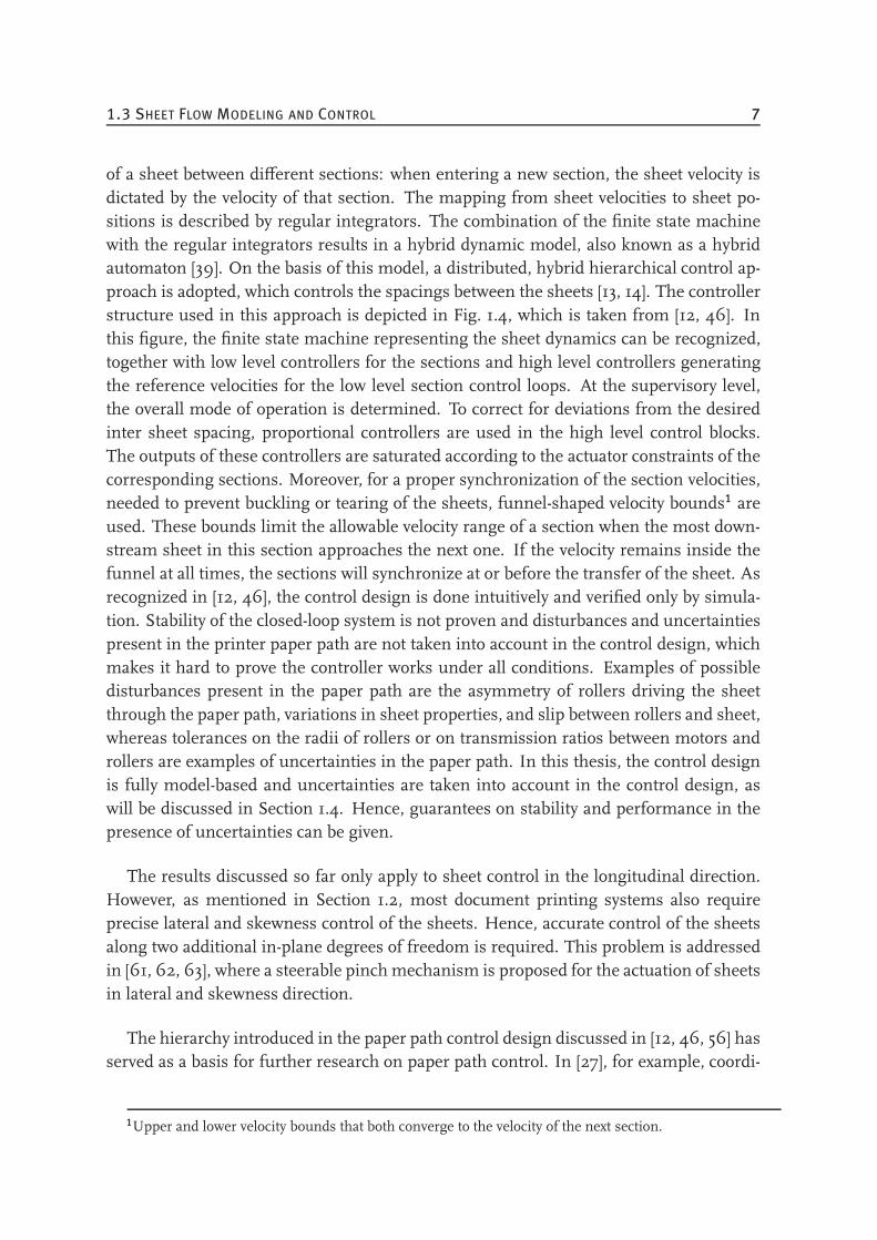
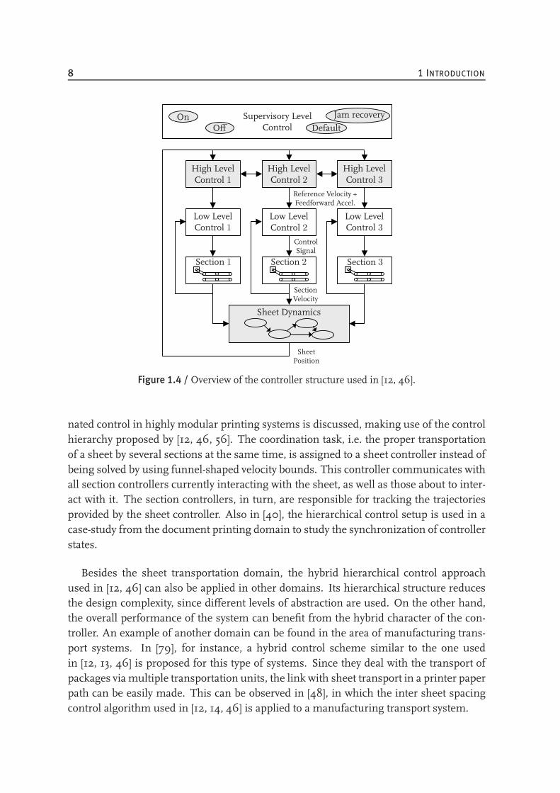
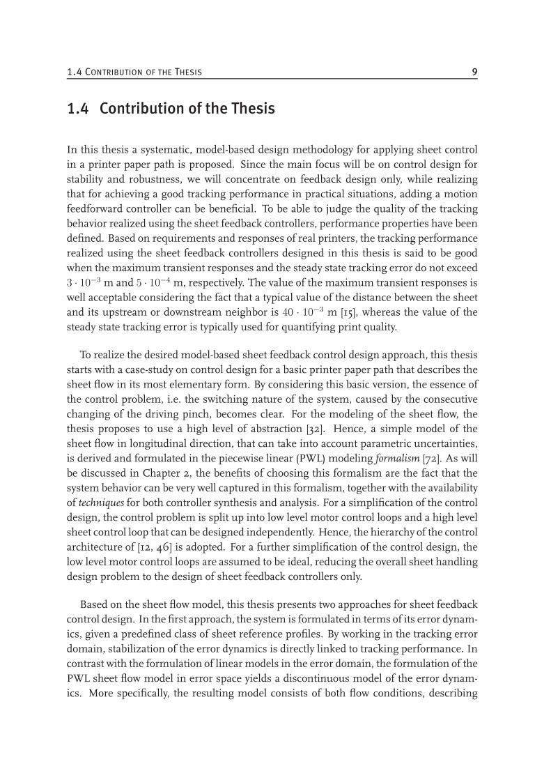
of a sheet between different sections: when entering a new section, the sheet velocity isdictated by the velocity of that section. The mapping from sheet velocities to sheet po-sitions is described by regular integrators. The combination of the finite state machinewith the regular integrators results in a hybrid dynamic model, also known as a hybridautomaton [39]. On the basis of this model, a distributed, hybrid hierarchical control ap-proach is adopted, which controls the spacings between the sheets [13, 14]. The controllerstructure used in this approach is depicted in Fig. 1.4, which is taken from [12, 46]. Inthis figure, the finite state machine representing the sheet dynamics can be recognized,together with low level controllers for the sections and high level controllers generatingthe reference velocities for the low level section control loops. At the supervisory level,the overall mode of operation is determined. To correct for deviations from the desiredinter sheet spacing, proportional controllers are used in the high level control blocks.The outputs of these controllers are saturated according to the actuator constraints of thecorresponding sections. Moreover, for a proper synchronization of the section velocities,needed to prevent buckling or tearing of the sheets, funnel-shaped velocity bounds1 areused. These bounds limit the allowable velocity range of a section when the most down-stream sheet in this section approaches the next one. If the velocity remains inside thefunnel at all times, the sections will synchronize at or before the transfer of the sheet. Asrecognized in [12, 46], the control design is done intuitively and verified only by simula-tion. Stability of the closed-loop system is not proven and disturbances and uncertaintiespresent in the printer paper path are not taken into account in the control design, whichmakes it hard to prove the controller works under all conditions. Examples of possibledisturbances present in the paper path are the asymmetry of rollers driving the sheetthrough the paper path, variations in sheet properties, and slip between rollers and sheet,whereas tolerances on the radii of rollers or on transmission ratios between motors androllers are examples of uncertainties in the paper path. In this thesis, the control designis fully model-based and uncertainties are taken into account in the control design, aswill be discussed in Section 1.4. Hence, guarantees on stability and performance in thepresence of uncertainties can be given.
The results discussed so far only apply to sheet control in the longitudinal direction.However, as mentioned in Section 1.2, most document printing systems also requireprecise lateral and skewness control of the sheets. Hence, accurate control of the sheetsalong two additional in-plane degrees of freedom is required. This problem is addressedin [61, 62, 63], where a steerable pinchmechanism is proposed for the actuation of sheetsin lateral and skewness direction.
The hierarchy introduced in the paper path control design discussed in [12, 46, 56] hasserved as a basis for further research on paper path control. In [27], for example, coordi-
1Upper and lower velocity bounds that both converge to the velocity of the next section.
8 1 INTRODUCTION
High LevelControl 1
High LevelControl 2
High LevelControl 3
Low LevelControl 1
Low LevelControl 2
Low LevelControl 3
Section 1 Section 2 Section 3
Sheet Dynamics
Reference Velocity +Feedforward Accel.
ControlSignal
SectionVelocity
SheetPosition
Supervisory LevelControl
OnOff
Jam recovery
Default
Figure 1.4 / Overview of the controller structure used in [12, 46].
nated control in highly modular printing systems is discussed, making use of the controlhierarchy proposed by [12, 46, 56]. The coordination task, i.e. the proper transportationof a sheet by several sections at the same time, is assigned to a sheet controller instead ofbeing solved by using funnel-shaped velocity bounds. This controller communicates withall section controllers currently interacting with the sheet, as well as those about to inter-act with it. The section controllers, in turn, are responsible for tracking the trajectoriesprovided by the sheet controller. Also in [40], the hierarchical control setup is used in acase-study from the document printing domain to study the synchronization of controllerstates.
Besides the sheet transportation domain, the hybrid hierarchical control approachused in [12, 46] can also be applied in other domains. Its hierarchical structure reducesthe design complexity, since different levels of abstraction are used. On the other hand,the overall performance of the system can benefit from the hybrid character of the con-troller. An example of another domain can be found in the area of manufacturing trans-port systems. In [79], for instance, a hybrid control scheme similar to the one usedin [12, 13, 46] is proposed for this type of systems. Since they deal with the transport ofpackages via multiple transportation units, the link with sheet transport in a printer paperpath can be easily made. This can be observed in [48], in which the inter sheet spacingcontrol algorithm used in [12, 14, 46] is applied to a manufacturing transport system.
1.4 CONTRIBUTION OF THE THESIS 9
1.4 Contribution of the Thesis
In this thesis a systematic, model-based design methodology for applying sheet controlin a printer paper path is proposed. Since the main focus will be on control design forstability and robustness, we will concentrate on feedback design only, while realizingthat for achieving a good tracking performance in practical situations, adding a motionfeedforward controller can be beneficial. To be able to judge the quality of the trackingbehavior realized using the sheet feedback controllers, performance properties have beendefined. Based on requirements and responses of real printers, the tracking performancerealized using the sheet feedback controllers designed in this thesis is said to be goodwhen the maximum transient responses and the steady state tracking error do not exceed3 · 10−3 m and 5 · 10−4 m, respectively. The value of the maximum transient responses iswell acceptable considering the fact that a typical value of the distance between the sheetand its upstream or downstream neighbor is 40 · 10−3 m [15], whereas the value of thesteady state tracking error is typically used for quantifying print quality.
To realize the desired model-based sheet feedback control design approach, this thesisstarts with a case-study on control design for a basic printer paper path that describes thesheet flow in its most elementary form. By considering this basic version, the essence ofthe control problem, i.e. the switching nature of the system, caused by the consecutivechanging of the driving pinch, becomes clear. For the modeling of the sheet flow, thethesis proposes to use a high level of abstraction [32]. Hence, a simple model of thesheet flow in longitudinal direction, that can take into account parametric uncertainties,is derived and formulated in the piecewise linear (PWL) modeling formalism [72]. As willbe discussed in Chapter 2, the benefits of choosing this formalism are the fact that thesystem behavior can be very well captured in this formalism, together with the availabilityof techniques for both controller synthesis and analysis. For a simplification of the controldesign, the control problem is split up into low level motor control loops and a high levelsheet control loop that can be designed independently. Hence, the hierarchy of the controlarchitecture of [12, 46] is adopted. For a further simplification of the control design, thelow level motor control loops are assumed to be ideal, reducing the overall sheet handlingdesign problem to the design of sheet feedback controllers only.
Based on the sheet flow model, this thesis presents two approaches for sheet feedbackcontrol design. In the first approach, the system is formulated in terms of its error dynam-ics, given a predefined class of sheet reference profiles. By working in the tracking errordomain, stabilization of the error dynamics is directly linked to tracking performance. Incontrast with the formulation of linear models in the error domain, the formulation of thePWL sheet flow model in error space yields a discontinuous model of the error dynam-ics. More specifically, the resulting model consists of both flow conditions, describing
10 1 INTRODUCTION
the dynamics in each regime, and jump conditions, describing the error dynamics at theswitching boundaries. Given the model in error space, a stabilizing state feedback controllaw is proposed. Rendering the zero tracking error situation an equilibrium of the errordynamics imposes a restriction on the admissible controllers, i.e. controllers that result ineither full or partial linearization of the systemmust be synthesized to realize the desiredequilibrium. Given the control law, relations between the type of controller and the typeof Lyapunov function needed for the stability analysis are derived. The actual calculationof the controller gains is carried out by solving a set of linear matrix inequalities (LMIs).For the case parameter uncertainties are present in the system, both the flow conditionsand the jump conditions are derived. Based on the latter conditions, an analysis for pre-dicting the effect of the uncertainties on the sheet tracking error is carried out. In thesecond control design approach, dynamic output feedback controllers are directly synthe-sized based on the switching sheet flow dynamics. The synthesis is also formulated interms of a set of LMIs and combines linear H∞ control design techniques for the indi-vidual regimes of the sheet flow dynamics with stability and performance requirementsfor the overall switched system. Initially, control design based on the nominal sheet flowmodel is considered, after which the approach is extended to take into account parametricmodel uncertainties within a prespecified bound, yielding controllers that result in bothrobust stability and robust performance of the switched closed-loop system.
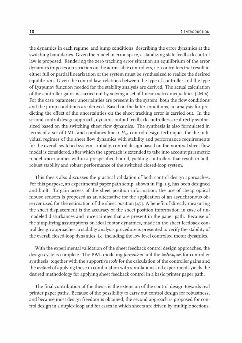
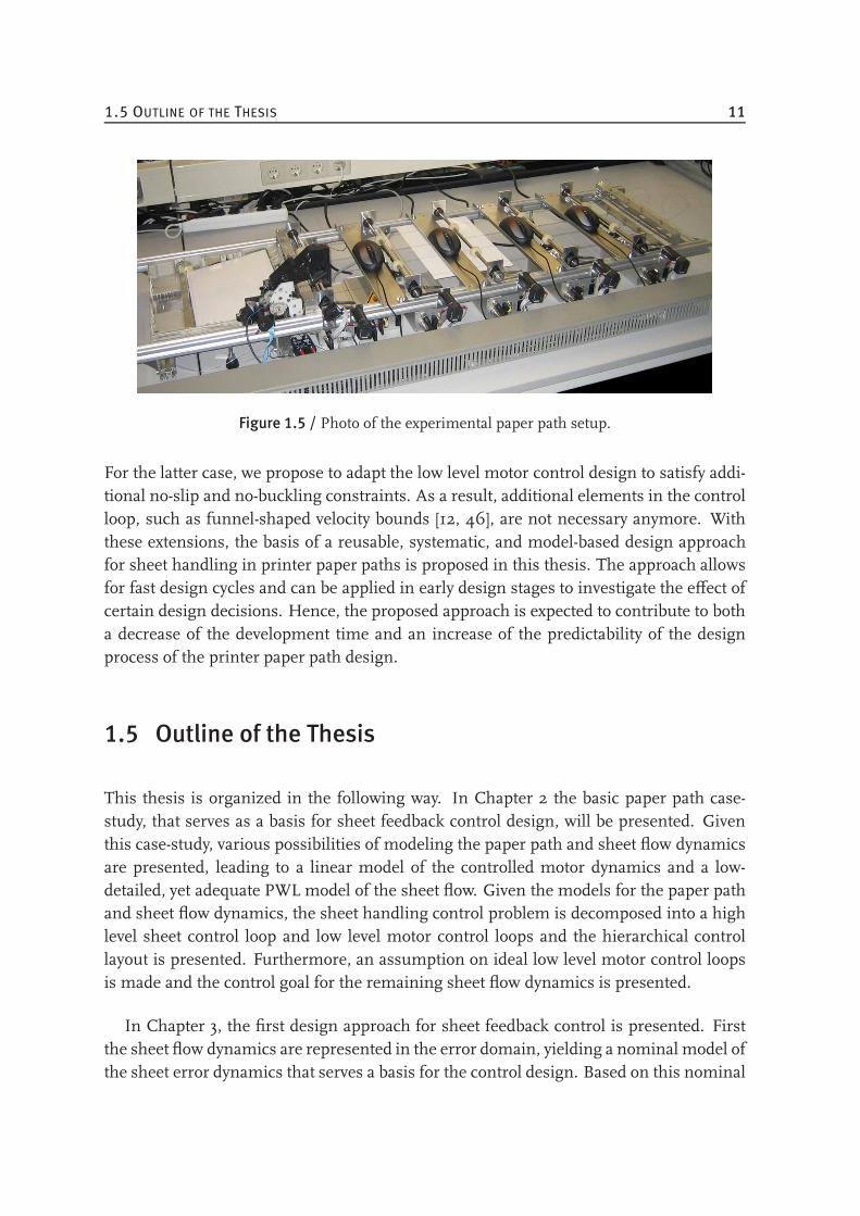
This thesis also discusses the practical validation of both control design approaches.For this purpose, an experimental paper path setup, shown in Fig. 1.5, has been designedand built. To gain access of the sheet position information, the use of cheap opticalmouse sensors is proposed as an alternative for the application of an asynchronous ob-server used for the estimation of the sheet position [47]. A benefit of directly measuringthe sheet displacement is the accuracy of the sheet position information in case of un-modeled disturbances and uncertainties that are present in the paper path. Because ofthe simplifying assumptions on ideal motor dynamics, made in the sheet feedback con-trol design approaches, a stability analysis procedure is presented to verify the stability ofthe overall closed-loop dynamics, i.e. including the low level controlled motor dynamics.
With the experimental validation of the sheet feedback control design approaches, thedesign cycle is complete. The PWL modeling formalism and the techniques for controllersynthesis, together with the supportive tools for the calculation of the controller gains andthemethod of applying these in combination with simulations and experiments yields thedesired methodology for applying sheet feedback control in a basic printer paper path.
The final contribution of the thesis is the extension of the control design towards realprinter paper paths. Because of the possibility to carry out control design for robustness,and because most design freedom is obtained, the second approach is proposed for con-trol design in a duplex loop and for cases in which sheets are driven by multiple sections.
1.5 OUTLINE OF THE THESIS 11
Figure 1.5 / Photo of the experimental paper path setup.
For the latter case, we propose to adapt the low level motor control design to satisfy addi-tional no-slip and no-buckling constraints. As a result, additional elements in the controlloop, such as funnel-shaped velocity bounds [12, 46], are not necessary anymore. Withthese extensions, the basis of a reusable, systematic, and model-based design approachfor sheet handling in printer paper paths is proposed in this thesis. The approach allowsfor fast design cycles and can be applied in early design stages to investigate the effect ofcertain design decisions. Hence, the proposed approach is expected to contribute to botha decrease of the development time and an increase of the predictability of the designprocess of the printer paper path design.
1.5 Outline of the Thesis
This thesis is organized in the following way. In Chapter 2 the basic paper path case-study, that serves as a basis for sheet feedback control design, will be presented. Giventhis case-study, various possibilities of modeling the paper path and sheet flow dynamicsare presented, leading to a linear model of the controlled motor dynamics and a low-detailed, yet adequate PWL model of the sheet flow. Given the models for the paper pathand sheet flow dynamics, the sheet handling control problem is decomposed into a highlevel sheet control loop and low level motor control loops and the hierarchical controllayout is presented. Furthermore, an assumption on ideal low level motor control loopsis made and the control goal for the remaining sheet flow dynamics is presented.
In Chapter 3, the first design approach for sheet feedback control is presented. Firstthe sheet flow dynamics are represented in the error domain, yielding a nominal model ofthe sheet error dynamics that serves a basis for the control design. Based on this nominal
12 1 INTRODUCTION
model, two types of controllers are proposed. The relation between the feedback con-trollers and the type of Lyapunov function for proving the stability of the closed-loop sys-tem is analyzed, together with the effect of parameter perturbations on the sheet trackingerror. Simulations are carried out for the validation of the synthesis and analysis results.
The second approach for sheet feedback control design is presented in Chapter 4.Based on models of the sheet flow dynamics, control designs for both the nominal caseand the case in which parametric uncertainties are present are discussed. Also for thiscontrol design approach, simulations are carried out. Furthermore, a procedure for thestability analysis of the overall system, i.e. including a model of the controlled motordynamics, is derived.
Chapter 5 presents the experimental setup used for the practical validation of the con-trol design approaches. The selection of a appropriate sensor for obtaining the sheetposition information is discussed, yielding optical mouse sensors as the most suitableoption. After describing the calibration procedure, the derivation of the sheet positioninformation from multiple sensors is discussed.
In Chapter 6, the results of the validation experiments are presented. First the dynam-ics of the motor-pinch combinations are identified. Based on measured data, models aredesigned that need to be taken into account in the stability analysis of the overall system.Furthermore, suitable feedback controllers for the low level motor-pinch systems are de-signed. The sheet feedback controllers obtained from both control design approaches areimplemented and the resulting responses are analyzed.
The extensions of sheet feedback control to industrial printer paper paths is discussedin Chapter 7. First the challenges in this type of paper paths are discussed, after whichthe second approach is chosen to be extended for application. Modeling and control ofthe sheet flow in a duplex loop are discussed, together with the case in which a sheet isdriven by multiple pinches. In the latter case, an adaptation of the low level motor controldesign is proposed, needed to take into account additional constraints imposed by thenew case.
Conclusions and recommendations regarding the work presented in this thesis arediscussed in Chapter 8.
CHAPTER TWO
The Sheet Feedback Control Architecture
2.1 Basic Paper Path Setup . . . . . . . . . . . . . . . . . . . . . . . . . . . . 13
2.2 Paper Path and Sheet Flow Modeling . . . . . . . . . . . . . . . . . . . . 14
2.3 Decomposition of the Sheet Handling Control Problem . . . . . . . . . 17
2.1 Basic Paper Path Setup
In this chapter the design of the architecture for model-based sheet feedback controllersynthesis is discussed. To understand the essence of the control problem, a case-studyis adopted that contains the most elementary elements present in a paper path. Giventhis case-study, the approach for modeling the sheet flow in the paper path is presented,resulting in a sheet flow model based on which the control design can be carried out. Tofacilitate this design, the sheet handling control problem is decomposed, resulting in amulti-level control hierarchy.
The case-study we adopt as a starting point for the design of the model-based sheethandling system is based on the most essential characteristic present in each printerpaper path, i.e. sheets being driven by motor-pinch combinations in a sequential man-ner. This leads to a basic paper path case-study that reveals the essence of the controlproblem, i.e. the switching nature of the system caused by the consecutive changing ofthe driving pinch. By considering this basic version, a number of characteristics presentin real printer paper paths, as the one shown in Fig. 1.3, are initially left out of consid-eration. The most important examples of these characteristics are the duplex loop forbackside printing, the grouping of pinches into sections, and the transport of sheets by
13
14 2 THE SHEET FEEDBACK CONTROL ARCHITECTURE
multiple pinches. Extensions to the basic paper path that include these characteristicswill be discussed in Chapter 7.
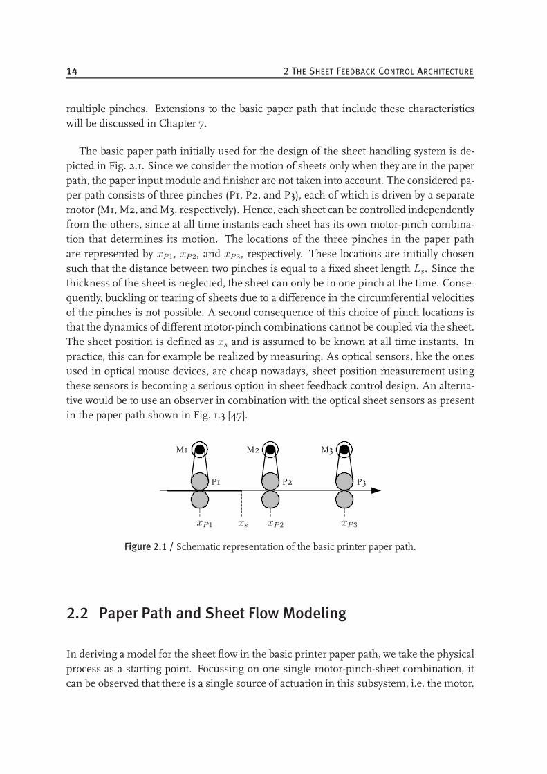
The basic paper path initially used for the design of the sheet handling system is de-picted in Fig. 2.1. Since we consider the motion of sheets only when they are in the paperpath, the paper input module and finisher are not taken into account. The considered pa-per path consists of three pinches (P1, P2, and P3), each of which is driven by a separatemotor (M1, M2, andM3, respectively). Hence, each sheet can be controlled independentlyfrom the others, since at all time instants each sheet has its own motor-pinch combina-tion that determines its motion. The locations of the three pinches in the paper pathare represented by xP1, xP2, and xP3, respectively. These locations are initially chosensuch that the distance between two pinches is equal to a fixed sheet length Ls. Since thethickness of the sheet is neglected, the sheet can only be in one pinch at the time. Conse-quently, buckling or tearing of sheets due to a difference in the circumferential velocitiesof the pinches is not possible. A second consequence of this choice of pinch locations isthat the dynamics of different motor-pinch combinations cannot be coupled via the sheet.The sheet position is defined as xs and is assumed to be known at all time instants. Inpractice, this can for example be realized by measuring. As optical sensors, like the onesused in optical mouse devices, are cheap nowadays, sheet position measurement usingthese sensors is becoming a serious option in sheet feedback control design. An alterna-tive would be to use an observer in combination with the optical sheet sensors as presentin the paper path shown in Fig. 1.3 [47].
M1 M2 M3
P1 P2 P3
xP1 xP2 xP3xs
Figure 2.1 / Schematic representation of the basic printer paper path.
2.2 Paper Path and Sheet Flow Modeling
In deriving a model for the sheet flow in the basic printer paper path, we take the physicalprocess as a starting point. Focussing on one single motor-pinch-sheet combination, itcan be observed that there is a single source of actuation in this subsystem, i.e. the motor.
2.2 PAPER PATH AND SHEET FLOW MODELING 15
This motor is coupled to the driven roller of the pinch via a gear belt and therefore themotion of the driven roller is determined by the motor. The second coupling is presentbetween the driven roller of the pinch and the sheet and therefore the sheet motion isdetermined by this driven roller. The non-driven roller of the pinch contributes in thetransportation of the sheet by applying sufficient normal force to prevent the sheet fromslipping in the pinch.
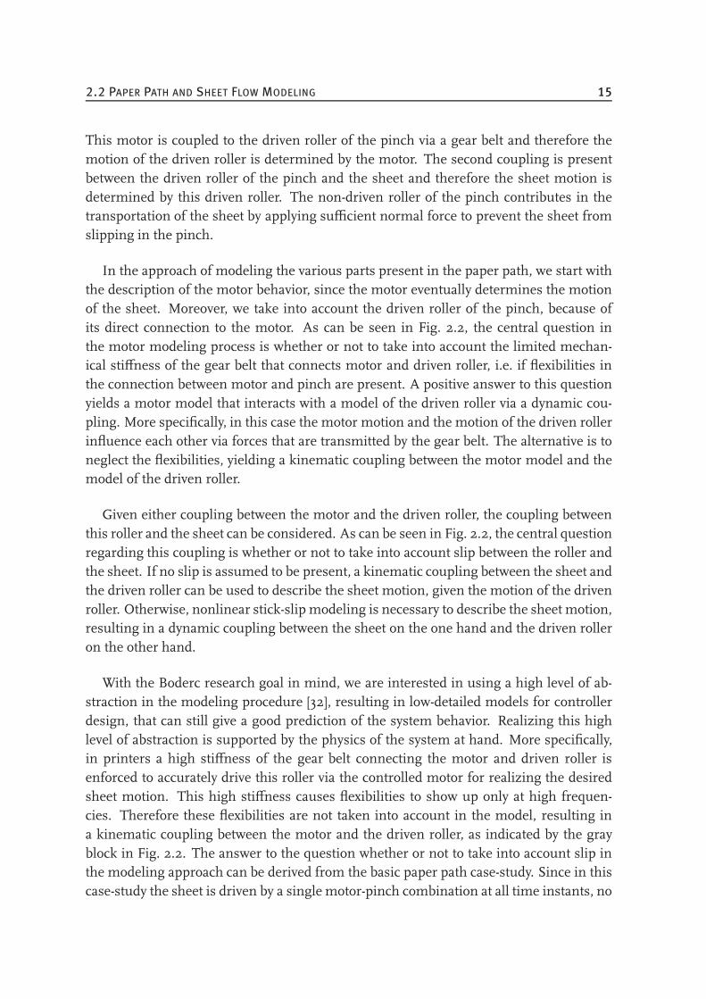
In the approach of modeling the various parts present in the paper path, we start withthe description of the motor behavior, since the motor eventually determines the motionof the sheet. Moreover, we take into account the driven roller of the pinch, because ofits direct connection to the motor. As can be seen in Fig. 2.2, the central question inthe motor modeling process is whether or not to take into account the limited mechan-ical stiffness of the gear belt that connects motor and driven roller, i.e. if flexibilities inthe connection between motor and pinch are present. A positive answer to this questionyields a motor model that interacts with a model of the driven roller via a dynamic cou-pling. More specifically, in this case the motor motion and the motion of the driven rollerinfluence each other via forces that are transmitted by the gear belt. The alternative is toneglect the flexibilities, yielding a kinematic coupling between the motor model and themodel of the driven roller.
Given either coupling between the motor and the driven roller, the coupling betweenthis roller and the sheet can be considered. As can be seen in Fig. 2.2, the central questionregarding this coupling is whether or not to take into account slip between the roller andthe sheet. If no slip is assumed to be present, a kinematic coupling between the sheet andthe driven roller can be used to describe the sheet motion, given the motion of the drivenroller. Otherwise, nonlinear stick-slip modeling is necessary to describe the sheet motion,resulting in a dynamic coupling between the sheet on the one hand and the driven rolleron the other hand.
With the Boderc research goal in mind, we are interested in using a high level of ab-straction in the modeling procedure [32], resulting in low-detailed models for controllerdesign, that can still give a good prediction of the system behavior. Realizing this highlevel of abstraction is supported by the physics of the system at hand. More specifically,in printers a high stiffness of the gear belt connecting the motor and driven roller isenforced to accurately drive this roller via the controlled motor for realizing the desiredsheet motion. This high stiffness causes flexibilities to show up only at high frequen-cies. Therefore these flexibilities are not taken into account in the model, resulting ina kinematic coupling between the motor and the driven roller, as indicated by the grayblock in Fig. 2.2. The answer to the question whether or not to take into account slip inthe modeling approach can be derived from the basic paper path case-study. Since in thiscase-study the sheet is driven by a single motor-pinch combination at all time instants, no
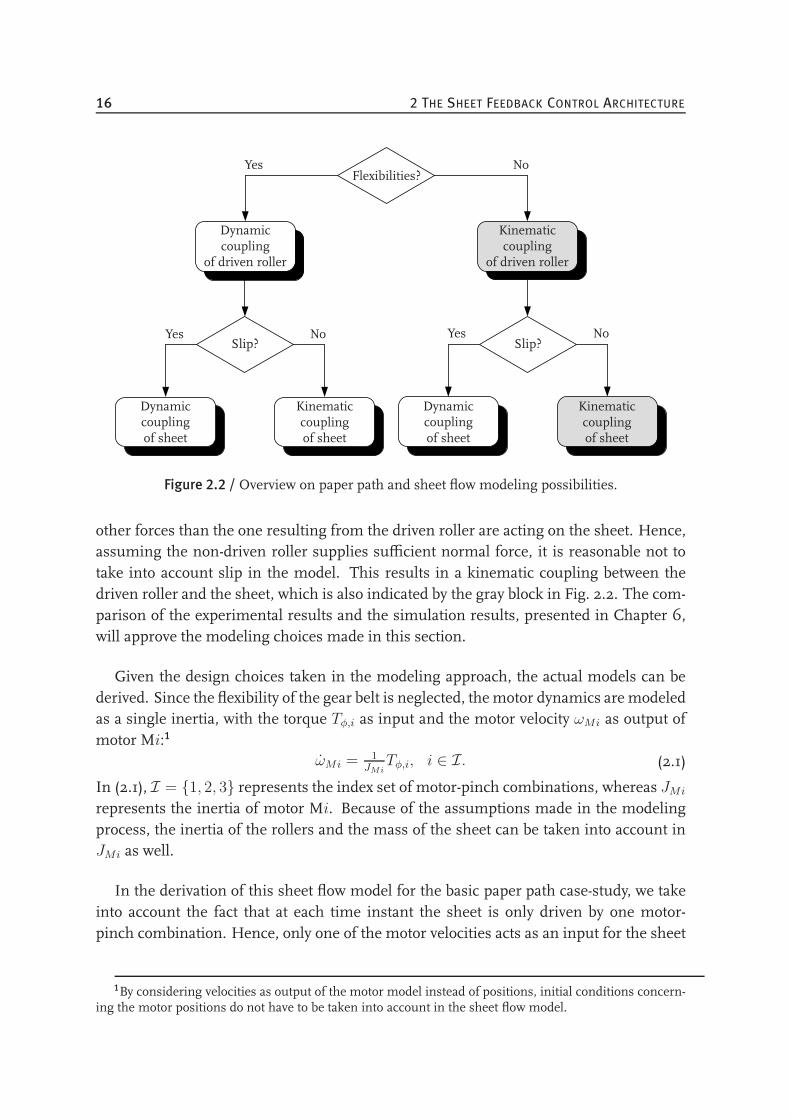
16 2 THE SHEET FEEDBACK CONTROL ARCHITECTURE
Flexibilities?
Dynamiccoupling
of driven roller
Kinematiccoupling
of driven roller
Slip?Slip?
Dynamiccouplingof sheet
Dynamiccouplingof sheet
Kinematiccouplingof sheet
Kinematiccouplingof sheet
Yes
Yes
Yes No
No
No
Figure 2.2 / Overview on paper path and sheet flow modeling possibilities.
other forces than the one resulting from the driven roller are acting on the sheet. Hence,assuming the non-driven roller supplies sufficient normal force, it is reasonable not totake into account slip in the model. This results in a kinematic coupling between thedriven roller and the sheet, which is also indicated by the gray block in Fig. 2.2. The com-parison of the experimental results and the simulation results, presented in Chapter 6,will approve the modeling choices made in this section.
Given the design choices taken in the modeling approach, the actual models can bederived. Since the flexibility of the gear belt is neglected, themotor dynamics are modeledas a single inertia, with the torque Tφ,i as input and the motor velocity ωMi as output ofmotor Mi:1
ωMi = 1JMi
Tφ,i, i ∈ I. (2.1)
In (2.1), I = 1, 2, 3 represents the index set of motor-pinch combinations, whereas JMi
represents the inertia of motor Mi. Because of the assumptions made in the modelingprocess, the inertia of the rollers and the mass of the sheet can be taken into account inJMi as well.
In the derivation of this sheet flow model for the basic paper path case-study, we takeinto account the fact that at each time instant the sheet is only driven by one motor-pinch combination. Hence, only one of the motor velocities acts as an input for the sheet
1By considering velocities as output of the motor model instead of positions, initial conditions concern-ing the motor positions do not have to be taken into account in the sheet flow model.
2.3 DECOMPOSITION OF THE SHEET HANDLING CONTROL PROBLEM 17
motion. As the sheet moves through the paper path, this input will change when thesheet arrives at the next pinch. This switching behavior can be easily captured in thePWL modeling formalism [72]. In the resulting sheet flow model, the mass of the sheetis not taken into account, as the effect of this mass is negligible with respect to the effectof the inertia of themotor-pinch combinations. Since flexibilities of the gear belts and slipbetween the sheet and the pinches are also not taken into account, the sheet velocity canbe derived from the motor velocities via straightforward holonomic kinematic constraintrelations that describe the relation between motor velocity and pinch velocity, and pinchvelocity and sheet velocity, respectively. The sheet position is obtained by integratingthe sheet velocity. The nominal high level sheet model, i.e. the sheet model withoutparameter uncertainties and disturbances, therefore consists of a switching integratorthat can be represented as
xs = Biu for xs ∈ Xi, i ∈ I, (2.2)
with the input matrices Bi defined as B1 =[n1rP1 0 0
], B2 =
[0 n2rP2 0
],
and B3 =[
0 0 n3rP3
], respectively. In these definitions, ni represents the trans-
mission ratio between motor Mi and pinch Pi and rPi represents the radius of thedriven roller of pinch i. Furthermore, u is the column with inputs of the high levelsheet dynamics: u =
[ωM1 ωM2 ωM3
]T. The partitioning of the state space into
the three regions is represented by Xii∈I ⊆ R. Here, X1 = xs|xs ∈ [xP1, xP2),X2 = xs|xs ∈ [xP2, xP3), and X3 = xs|xs ∈ [xP3, xP3 + Ls), since xP2 − xP1 = Lsand xP3 − xP2 = Ls.
2.3 Decomposition of the Sheet Handling Control Problem
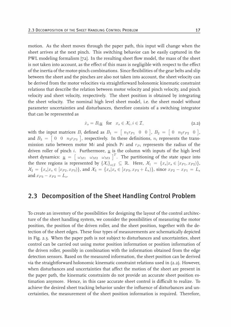
To create an inventory of the possibilities for designing the layout of the control architec-ture of the sheet handling system, we consider the possibilities of measuring the motorposition, the position of the driven roller, and the sheet position, together with the de-tection of the sheet edges. These four types of measurements are schematically depictedin Fig. 2.3. When the paper path is not subject to disturbances and uncertainties, sheetcontrol can be carried out using motor position information or position information ofthe driven roller, possibly in combination with the information obtained from the edgedetection sensors. Based on the measured information, the sheet position can be derivedvia the straightforward holonomic kinematic constraint relations used in (2.2). However,when disturbances and uncertainties that affect the motion of the sheet are present inthe paper path, the kinematic constraints do not provide an accurate sheet position es-timation anymore. Hence, in this case accurate sheet control is difficult to realize. Toachieve the desired sheet tracking behavior under the influence of disturbances and un-certainties, the measurement of the sheet position information is required. Therefore,
18 2 THE SHEET FEEDBACK CONTROL ARCHITECTURE
we consider the following three options of using position information for controlling thesheet flow:
1. sheet control based on the measurement of the sheet position information only,
2. sheet control based on the measurement of both the motor position and the sheetposition,
3. and sheet control based on the measurement of both the position of the drivenroller and the sheet position.
When option 1 is chosen for implementation, a control problem can be obtained in whichthe goal is to find a single controller for the combination of the motor, the driven roller,and the sheet. In contrast with this option, options 2 and 3 allow us to split up thesheet handling control problem into two levels, as done in [12, 46]. At the low level,model-based collocated (option 2) or non-collocated (option 3) motor control design isconsidered, whereas on the high level the focus is on model-based control of the sheetflow. This subdivision is possible since both the sheet position and the position of themotor or the driven roller are available and because of the no-slip condition between thepinch and the sheet. Breaking up the control problem into two parts seems natural forthe system at hand and replaces the overall design question by two separate, less com-plex, control questions. Hence, options 2 and 3 are preferred over option 1. Since ina non-collocated control architecture high bandwidths are more difficult to realize thanin collocated control architectures, collocated motor control is preferred. Moreover, con-sidering the application of sheet feedback control in real printer paper paths, in whichpinches are often coupled into sections that are driven by a single motor, option 2 is alsopreferred over option 3. This results from a technical point of view on the one hand, i.e.switching between position information would be needed in option 3 as the sheet is trans-ported through the section, and from an economical point of view on the other hand, i.e.less encoders are needed in option 2, resulting in a less expensive printer. Hence, in thisthesis option 2 is chosen as a basis for controlling the sheet flow.
Measure Motor Position
Measure Position of Driven Roller
Measure Sheet Position
Edge Detection
Figure 2.3 / Four possibilities for measuring: the motor position, the position of the drivenroller, the sheet position, and the detection of the edge of the sheet.
2.3 DECOMPOSITION OF THE SHEET HANDLING CONTROL PROBLEM 19
The low level motor control loops are used to tackle disturbances and uncertainties atthe motor level, e.g. cogging and friction in the bearings. In many cases, the controlledmotor dynamics can be very well described by a linear model. Hence, each motor controlloop in the paper path can be designed on the basis of well-known linear single-inputsingle-output motion control techniques [25]. The closed-loop linear motor dynamics inthe Laplace domain can be represented by
ΩMi(s) = Ti(s)ΩMi,r(s), i ∈ I, (2.3)
when assuming zero initial conditions. In (2.3), Ti(s) represents the complementary sen-sitivity function of controlledmotor Mi, which maps the input of the low level closed-loopsystem, i.e. the motor reference velocity ωMi,r, with ωMi,r the inverse Laplace transformof ΩMi,r(s), s ∈ C, to its output, i.e. the actual motor velocity ωMi, with Laplace transformΩMi(s).
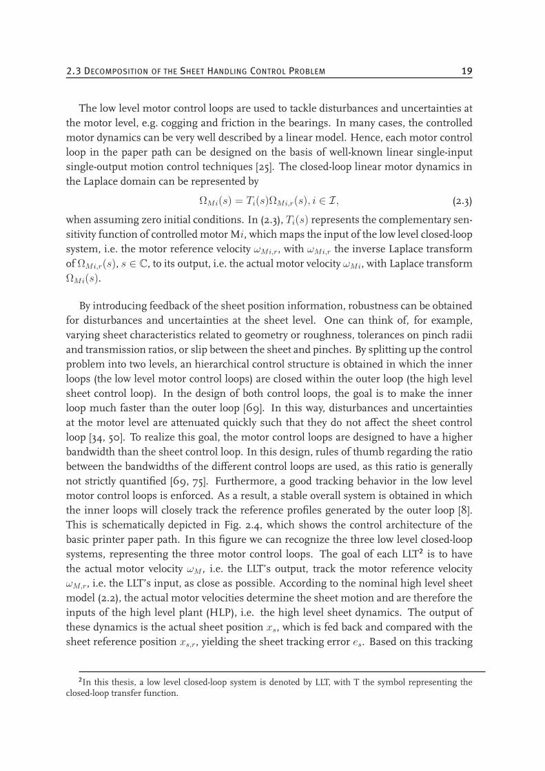
By introducing feedback of the sheet position information, robustness can be obtainedfor disturbances and uncertainties at the sheet level. One can think of, for example,varying sheet characteristics related to geometry or roughness, tolerances on pinch radiiand transmission ratios, or slip between the sheet and pinches. By splitting up the controlproblem into two levels, an hierarchical control structure is obtained in which the innerloops (the low level motor control loops) are closed within the outer loop (the high levelsheet control loop). In the design of both control loops, the goal is to make the innerloop much faster than the outer loop [69]. In this way, disturbances and uncertaintiesat the motor level are attenuated quickly such that they do not affect the sheet controlloop [34, 50]. To realize this goal, the motor control loops are designed to have a higherbandwidth than the sheet control loop. In this design, rules of thumb regarding the ratiobetween the bandwidths of the different control loops are used, as this ratio is generallynot strictly quantified [69, 75]. Furthermore, a good tracking behavior in the low levelmotor control loops is enforced. As a result, a stable overall system is obtained in whichthe inner loops will closely track the reference profiles generated by the outer loop [8].This is schematically depicted in Fig. 2.4, which shows the control architecture of thebasic printer paper path. In this figure we can recognize the three low level closed-loopsystems, representing the three motor control loops. The goal of each LLT2 is to havethe actual motor velocity ωM , i.e. the LLT’s output, track the motor reference velocityωM,r, i.e. the LLT’s input, as close as possible. According to the nominal high level sheetmodel (2.2), the actual motor velocities determine the sheet motion and are therefore theinputs of the high level plant (HLP), i.e. the high level sheet dynamics. The output ofthese dynamics is the actual sheet position xs, which is fed back and compared with thesheet reference position xs,r, yielding the sheet tracking error es. Based on this tracking
2In this thesis, a low level closed-loop system is denoted by LLT, with T the symbol representing theclosed-loop transfer function.
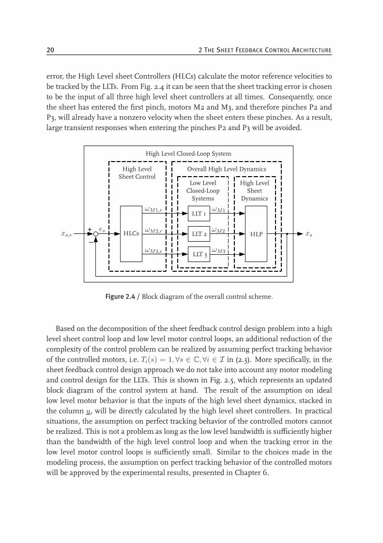
20 2 THE SHEET FEEDBACK CONTROL ARCHITECTURE
error, the High Level sheet Controllers (HLCs) calculate the motor reference velocities tobe tracked by the LLTs. From Fig. 2.4 it can be seen that the sheet tracking error is chosento be the input of all three high level sheet controllers at all times. Consequently, oncethe sheet has entered the first pinch, motors M2 and M3, and therefore pinches P2 andP3, will already have a nonzero velocity when the sheet enters these pinches. As a result,large transient responses when entering the pinches P2 and P3 will be avoided.
+_
HLCs
LLT 1
LLT 2
LLT 3
HLP
ωM1,r
ωM2,r
ωM3,r
Low LevelClosed-LoopSystems
High LevelSheet
Dynamics
High LevelSheet Control
Overall High Level Dynamics
High Level Closed-Loop System
xs,r xs
ωM1
ωM2
ωM3
es
Figure 2.4 / Block diagram of the overall control scheme.
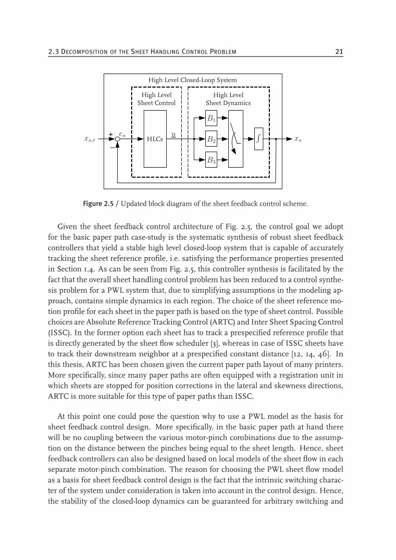
Based on the decomposition of the sheet feedback control design problem into a highlevel sheet control loop and low level motor control loops, an additional reduction of thecomplexity of the control problem can be realized by assuming perfect tracking behaviorof the controlled motors, i.e. Ti(s) = 1, ∀s ∈ C, ∀i ∈ I in (2.3). More specifically, in thesheet feedback control design approach we do not take into account any motor modelingand control design for the LLTs. This is shown in Fig. 2.5, which represents an updatedblock diagram of the control system at hand. The result of the assumption on ideallow level motor behavior is that the inputs of the high level sheet dynamics, stacked inthe column u, will be directly calculated by the high level sheet controllers. In practicalsituations, the assumption on perfect tracking behavior of the controlled motors cannotbe realized. This is not a problem as long as the low level bandwidth is sufficiently higherthan the bandwidth of the high level control loop and when the tracking error in thelow level motor control loops is sufficiently small. Similar to the choices made in themodeling process, the assumption on perfect tracking behavior of the controlled motorswill be approved by the experimental results, presented in Chapter 6.
2.3 DECOMPOSITION OF THE SHEET HANDLING CONTROL PROBLEM 21
+_
HLCs
B1
B2
B3
u ∫
High LevelSheet Dynamics
High LevelSheet Control
High Level Closed-Loop System
xs,r xses
Figure 2.5 / Updated block diagram of the sheet feedback control scheme.
Given the sheet feedback control architecture of Fig. 2.5, the control goal we adoptfor the basic paper path case-study is the systematic synthesis of robust sheet feedbackcontrollers that yield a stable high level closed-loop system that is capable of accuratelytracking the sheet reference profile, i.e. satisfying the performance properties presentedin Section 1.4. As can be seen from Fig. 2.5, this controller synthesis is facilitated by thefact that the overall sheet handling control problem has been reduced to a control synthe-sis problem for a PWL system that, due to simplifying assumptions in the modeling ap-proach, contains simple dynamics in each region. The choice of the sheet reference mo-tion profile for each sheet in the paper path is based on the type of sheet control. Possiblechoices are Absolute Reference Tracking Control (ARTC) and Inter Sheet Spacing Control(ISSC). In the former option each sheet has to track a prespecified reference profile thatis directly generated by the sheet flow scheduler [3], whereas in case of ISSC sheets haveto track their downstream neighbor at a prespecified constant distance [12, 14, 46]. Inthis thesis, ARTC has been chosen given the current paper path layout of many printers.More specifically, since many paper paths are often equipped with a registration unit inwhich sheets are stopped for position corrections in the lateral and skewness directions,ARTC is more suitable for this type of paper paths than ISSC.
At this point one could pose the question why to use a PWL model as the basis forsheet feedback control design. More specifically, in the basic paper path at hand therewill be no coupling between the various motor-pinch combinations due to the assump-tion on the distance between the pinches being equal to the sheet length. Hence, sheetfeedback controllers can also be designed based on local models of the sheet flow in eachseparate motor-pinch combination. The reason for choosing the PWL sheet flow modelas a basis for sheet feedback control design is the fact that the intrinsic switching charac-ter of the system under consideration is taken into account in the control design. Hence,the stability of the closed-loop dynamics can be guaranteed for arbitrary switching and

22 2 THE SHEET FEEDBACK CONTROL ARCHITECTURE
performance and robustness guarantees can be given for the overall system, i.e. the sheetmotion in the complete paper path, which can in general not be done using individualdesigns only. Moreover, a generic framework is obtained, which can be used for extendedproblem formulations. Given this motivation, two approaches for controller synthesisbased on the PWL model of the sheet flow will be presented in Chapters 3 and 4.
CHAPTER THREE
State Feedback Control Design
3.1 The Tracking Control Problem . . . . . . . . . . . . . . . . . . . . . . . 23
3.2 Nominal Sheet Feedback Control Design . . . . . . . . . . . . . . . . . . 26
3.3 Analysis of the Perturbation of Paper Path Parameters . . . . . . . . . . 41
3.4 Evaluation . . . . . . . . . . . . . . . . . . . . . . . . . . . . . . . . . . . 51
3.1 The Tracking Control Problem
This chapter presents the first approach for sheet feedback control design for the basicpaper path case-study presented in Section 2.1. The goal is to synthesize sheet feed-back controllers that make the sheets in the paper path track a reference trajectory thatis known a priori, satisfying the performance properties presented in Section 1.4. Tomeet these specifications in practical situations, the use of a motion feedforward con-troller can be beneficial. However, the focus in this thesis will be on control design forrobustness, and therefore we will concentrate on feedback design only. Initially, we willconcentrate on control design based on the nominal high level sheet model (2.2). Basedon this model, two synthesis approaches will be presented with which controllers can bedesigned that meet the desired performance properties. Given these controllers, the ef-fect of perturbations of the system parameters will be analyzed. Therefore, the nominalsheet flow model will be extended such that it includes parametric uncertainties presentin the paper path. Based on the resulting model, an analysis technique will be presentedthat enables the prediction of the increase in sheet position and velocity errors originatingfrom the parameter perturbations.
23
24 3 STATE FEEDBACK CONTROL DESIGN
Control design and analysis of PWL systems has been given much attention in liter-ature lately, see for example [19] for an overview. In [44], piecewise quadratic Lyapunovfunctions were proposed for the analysis of PWL systems. In [57], the use of piecewisequadratic cost functions is extended from stability analysis to performance analysis andoptimal control. In [35], analysis and controller synthesis of PWL systems is considered,based on constructing (piecewise) quadratic Lyapunov functions that prove stability andperformance of the system. It is shown that proving stability and performance, as well asdesigning controllers, can be expressed as convex optimization problems involving LMIs.The work is extended in [59] to obtain an iterative method that can be used to design stateand output feedback controllers with various constraints on the continuity and smooth-ness of the Lyapunov Function and control signals. In [23], an H∞ controller synthesismethod for PWL systems based on a piecewise smooth Lyapunov function is presented.A stabilizing controller is synthesized that results in disturbance attenuation up to a pre-scribed level. This work is extended in [11, 22] to be able to deal with uncertain PWLsystems. A regulation control problem is considered for which a control design approachis presented for the stabilization with H∞ performance of the closed-loop system. AnalternativeH∞ control design approach for uncertain PWL systems, that can be used forsolving tracking control problems, will be the subject of Chapter 4.
A common property of the work presented in [35, 44, 57, 59] is the focus on the stabi-lization of the system dynamics, i.e. regulation problems are considered, whereas track-ing control problems are given less attention, as recognized in [60, 71]. In our case,however, the goal is to have the sheets in the paper path track a reference trajectory thatis known a priori. Hence, we are dealing with a tracking problem and we will thereforeformulate the system in terms of its error dynamics. By working in the tracking error do-main, as is common for the linear case [25], stabilization of the error dynamics is directlylinked to tracking performance. Note that if a fast decay of transient error responses isdesired, one has to ensure that the equilibrium in error space is reached quickly. Hence,given a system formulation in terms of the error dynamics, the control goal becomesto find a feedback controller that results in regulation of the error dynamics, in such away that all error states go to zero with a prescribed convergence rate. This automat-ically implies that the actual sheet position will become equal to the desired one and,hence, the desired tracking performance can be obtained [8, 10]. Hence, the basic ideaof [35, 44, 57, 59], i.e. controller synthesis and stability analysis using a common or piece-wise quadratic Lyapunov function, will be applied in this chapter. However, as we willsee, formulation of the PWL sheet flow model in terms of its error dynamics will lead toa distinguishing feature, i.e. the introduction of jumps in the state variables.
For the derivation of the error dynamics of the nominal high level PWL sheetmodel (2.2), we use the error-space approach of [25] and extend it to the PWL case. As faras the sheet reference profile is concerned, needed in the derivation of the error dynam-

3.1 THE TRACKING CONTROL PROBLEM 25
ics, in real printer paper paths piecewise linear velocity profiles are commonly used. Inthis case, however, we will consider a first order sheet reference profile for simplicity tofocus on the essence of the resulting control problem. Hence, the second time derivativeof the sheet reference position, i.e. the sheet reference acceleration, is taken zero in thederivation of the sheet error dynamics:
xs,r = 0. (3.1)
The sheet tracking error is defined as the difference between the sheet reference positionand the actual sheet position:
es = xs,r − xs. (3.2)
Substitution of the nominal high level sheet model (2.2) in the time derivative of (3.2)yields
es = xs,r − xs= xs,r − Biu for xs,r − es ∈ Xi, i ∈ I.
(3.3)
Due to the switching character of the system, the right hand side of (3.3) can be discontin-uous. Therefore the model of the sheet error dynamics will consist of two parts: the flowconditions that hold for the error dynamics of the various subsystems and the jump con-ditions that describe the relation of both es and es just before and just after the switchingmoment.
For the derivation of the flow conditions, we differentiate (3.3) one more time, sincethen explicit dependencies on xs,r and its time derivatives vanish, yielding
es = −Biu for xs,r − es ∈ Xi, i ∈ I. (3.4)
Next, the time derivative of the control input u is replaced by the control input in error-space [25], which is defined as
µ = u. (3.5)
When we define the state vector of the error dynamics as
q =[es es
]T, (3.6)
we can write the flow conditions in error space in standard state-variable form:
q = Fq +Giµ for(xs,r −
[1 0
]q)∈ Xi, i ∈ I. (3.7)
In this notation, the system matrix is defined as F =
[0 10 0
], whereas the input matrix
is defined as Gi =[
0 −BTi
]T.
Regarding the jump conditions, the physical interpretation of the system at handshows that switching from regime k to regime k + 1 and vice versa is possible, with
26 3 STATE FEEDBACK CONTROL DESIGN
k ∈ K, K = 1, 2.1 When we consider the transition from regime k to regime k + 1, thefollowing relation holds for the sheet tracking error at the switching boundary:
e+s (ts) = e−s (ts), (3.8)
with e+s (ts) := limt↓ts es(t) and e−s (ts) := limt↑ts es(t), and with ts the switching time.From (3.8) it can be seen that es is continuous at the switching boundary, which is sup-ported by the physics of the system, as the sheet cannot make instantaneous jumps. Thejump conditions for es are derived from (3.3). For e+s (ts), the following relation holds:
e+s (ts) = xs,r(ts) −Bk+1u(ts), k ∈ K, (3.9)
whereas for e−s (ts) it holds that
e−s (ts) = xs,r(ts) −Bku(ts), k ∈ K. (3.10)
Subtraction of (3.10) from (3.9) yields the desired jump condition for es:
e+s (ts) = e−s (ts) + (Bk − Bk+1)u(ts), k ∈ K. (3.11)
Given (3.8) and (3.11), the jump conditions can be represented as
q+(ts) =
[1 00 1
]q−(ts) +
[0T
Bk − Bk+1
]u(ts), k ∈ K, (3.12)
with q−(ts) :=[e−s (ts) e−s (ts)
]Tand q+(ts) :=
[e+s (ts) e+s (ts)
]T.2 Hence, the com-
plete model of the open-loop sheet dynamics in error space is given by the flow condi-tions (3.7) and the jump conditions (3.12).
3.2 Nominal Sheet Feedback Control Design
3.2.1 Controller Synthesis
For controlling the piecewise linear flow dynamics in error space (3.7) in combinationwith the jump conditions (3.12), we propose a control law that is based on state feedbackof the error dynamics:
µ = −Kq, (3.13)
1For clarity, note that in this chapter the index k is used to indicate the regimes between which a transi-tion is made, whereas the index i is used to indicate the regimes in all other cases.
2Note that these particular jump conditions result from the assumptions made in the modeling process.If, for example, the mass would have been taken into account, slightly different jump conditions would havebeen obtained, as otherwise infinitely large forces would be needed to realize the jump in es, which is notrealistic.
3.2 NOMINAL SHEET FEEDBACK CONTROL DESIGN 27
with K the matrix with state feedback gains to be calculated. From (3.13), it can be seenthat the controller calculates the three control inputs of the high level sheet dynamics, i.e.the three motor reference velocities, independent of the location of the sheet in the paperpath, i.e. no regional information is used in the definition of the control law. Hence,the controller itself is not switching and the structure of the input matrices of the sheetflow dynamics makes sure that the correct control input influences the sheet motion.Substitution of (3.13) into (3.7) yields the closed-loop flow dynamics in error space:
q = (F −GiK) q for(xs,r −
[1 0
]q)∈ Xi, i ∈ I. (3.14)
For the derivation of the closed-loop jump conditions, first u is derived by substitutionof (3.13) into (3.5) and integration of the resulting equation. Hence, for each i-th elementof u, ui, the following relation holds:
ui(t) = −K(i, 1)
∫ t
t0
es(τ)dτ −K(i, 2)es(t), i ∈ I, (3.15)
with t0 the initial time, ui(t0) = 0, and K(i, j) the j-th element of the i-th row of K,j ∈ 1, 2. As can be seen from (3.15), the control law for each region consists of aproportional-integral (PI) controller.
The second step in deriving the closed-loop jump conditions is substitution of (3.15)into (3.11), yielding the closed-loop jump condition for es when considering the transitionfrom regime k to regime k + 1:
e+s (ts) = e−s (ts) −Bk(k)(K(k, 1)
∫ ts
t0es(τ)dτ +K(k, 2)es(ts)
)+
+Bk+1(k + 1)(K(k + 1, 1)
∫ tst0es(τ)dτ +K(k + 1, 2)es(ts)
), k ∈ K.
(3.16)In (3.16), Bk(k) represents the k-th element of Bk, i.e. its only nonzero element.Given (3.8) and (3.16), the closed-loop jump conditions can be represented as
q+(ts) =
[1 0
Bk+1(k + 1)K(k + 1, 2) −Bk(k)K(k, 2) 1
]q−(ts)+
+
[0
Bk+1(k + 1)K(k + 1, 1) − Bk(k)K(k, 1)
] ∫ ts
t0es(τ)dτ
= Rk,k+1q−(ts) +
[0
Bk+1(k + 1)K(k + 1, 1) −Bk(k)K(k, 1)
] ∫ ts
t0es(τ)dτ,
k ∈ K.(3.17)
From (3.17), it can be seen that if it is desired not to have jumps in es at the switchingboundaries, the controller gains should be chosen such that both Bk+1(k + 1)K(k +
1, 2) = Bk(k)K(k, 2) and Bk+1(k + 1)K(k + 1, 1) = Bk(k)K(k, 1). When the resulting
28 3 STATE FEEDBACK CONTROL DESIGN
controller is applied to the nominal high level sheet model (2.2), it can be seen that alinear closed-loop system is obtained, from which we can conclude that the controllerlinearizes the sheet dynamics. Furthermore, from (3.14) it can be seen that in this caseq = 0 is an equilibrium point of the closed-loop system. As q = 0 implies es = 0
and es = 0, this is the equilibrium point we are interested in. However, to ensure thatq = 0 is an equilibrium point, it is not necessary to enforce both Bk+1(k + 1)K(k +
1, 2) = Bk(k)K(k, 2) and Bk+1(k + 1)K(k + 1, 1) = Bk(k)K(k, 1). More specifically, theonly necessary condition for q = 0 to be an equilibrium point is that the second termof (3.17) is equal to 0, as can be seen from (3.14) and (3.17). Clearly, a sufficient conditionfor this to realize is Bk+1(k + 1)K(k + 1, 1) = Bk(k)K(k, 1) via the choice of K(k, 1)
and K(k + 1, 1). If the integral term in (3.17) is nonzero, which is to be expected inpractical cases, the above mentioned condition is also a necessary one. In other words,the feedback controllers (3.15) have to be at least partially linearizing to enforce the originto be a globally asymptotically stable equilibrium in the sense of Lyapunov. In summary,two types of controllers are considered:
• Fully linearizing controllers. To obtain this type of controllers, the gains should bechosen such that bothBk+1(k+1)K(k+1, 2) = Bk(k)K(k, 2) andBk+1(k+1)K(k+
1, 1) = Bk(k)K(k, 1). Given this type of controllers, q = 0 is an equilibrium pointof the closed-loop system and jumps in the error states will not occur.
• Partially linearizing controllers. To obtain this type of controllers, the gains shouldbe chosen such that Bk+1(k + 1)K(k + 1, 1) = Bk(k)K(k, 1). Given this type ofcontrollers, q = 0 is an equilibrium point of the closed-loop system and jumps ines will not be eliminated.
Regarding the partially linearizing controllers, more freedom in the choice of the con-troller parameters is obtained. As a result, the behavior of the system could be improvedor additional characteristics could be introduced. One could think of, for example, im-provement of the performance index containing the control input, as in LQR controlproblems [25, 69], or the possibility to design for different control bandwidths in thevarious subsystems.
Given a partially linearizing feedback controller, the expression for the closed-loopjump conditions becomes:
q+ = Rk,k+1q−, k ∈ K. (3.18)
In analogy with the derivation of (3.18), the closed-loop jump conditions can also be de-rived when the transition from regime k + 1 to regime k is considered, i.e. when thesystem switches back to the previous regime. This could occur, for example, in a regis-tration unit of a real printer paper path, or after a change in direction of motion of the
3.2 NOMINAL SHEET FEEDBACK CONTROL DESIGN 29
sheet when leaving the duplex loop. In this case, the expression for the closed-loop jumpconditions becomes:
q+ =
[1 0
Bk(k)K(k, 2) − Bk+1(k + 1)K(k + 1, 2) 1
]q−
= Rk+1,kq−, k ∈ K.
(3.19)
From (3.17) and (3.19) it can be observed that switching forward and backward has thesame influence on themagnitude of a jump, whereas the sign of the jump differs. Hence,Rk,k+1 and Rk+1,k are related via
Rk,k+1 = R−1k+1,k, k ∈ K. (3.20)
Focussing again on the transition from region k to region k+1, the stability analysis ofthe closed-loop error dynamics (3.14), (3.18) encompasses two parts: the stability analysisof the flow dynamics in each regime and the stability analysis at the switching bound-ary connecting two regimes. By making use of the work presented in [6, 19], it can beanalyzed whether the closed-loop flow dynamics in error space in (3.14) are Globally Ex-ponentially Stable (GES). By considering exponential stability, the rate of convergence ofthe tracking error to zero can be adjusted such that the performance properties presentedin Section 1.4 are satisfied. For the stability analysis, a piecewise quadratic Lyapunovfunction candidate is proposed:
Vi(q) = qTPiq, i ∈ I, (3.21)
withPi = P T
i ≻ 0, i ∈ I. (3.22)
To prove that the flow dynamics are GES, the following set of matrix inequalities in PiandK must hold:
0 ≻ Vi(q) + αVi(q) =
= (F −GiK)T Pi + Pi (F −GiK) + αPi, i ∈ I,(3.23)
with α > 0 representing the decay rate of the Lyapunov function. This parameter is cho-sen a priori in relation to the transient behavior of the error dynamics, and therefore inrelation to the desired tracking performance. A large value of α results in a fast conver-gence of the error to zero. However, it is possible that beyond some value of α, no feasiblesolution of (3.23) can be obtained anymore. From (3.23), it becomes clear that both thestability analysis of the flow dynamics and the calculation of the controller gains K canbe carried out by solving a single set of matrix inequalities. In other words, the free pa-rameters to be solved, i.e. the Lyapunov matrices Pi and the matrix with controller gainsK, depend on each other.
30 3 STATE FEEDBACK CONTROL DESIGN
This dependency is also present in the stability analysis at the switching boundaryconnecting two regimes. To characterize the dependency, we consider both the transitionfrom regime k to regime k + 1 and vice versa. In both transitions, no extra energy isallowed to enter the system, i.e. the Lyapunov function active in a new regime must besmaller than or equal to the Lyapunov function active in the previous regime. Keepingthis in mind, we start with the transition from regime k to regime k + 1, and we require:
(q+)TPk+1q+ ≤ (q−)TPkq
−, k ∈ K. (3.24)
To show the relation between Pi and the controller parameters, two inequalities describ-ing the relation between Pk, Pk+1, Rk,k+1, and Rk+1,k can be derived from (3.24) bymaking use of the closed-loop jump conditions (3.18). First of all, (3.18) is substitutedinto (3.24) to obtain a relation between Pk, Pk+1, and Rk,k+1:
(q−)TRTk,k+1Pk+1Rk,k+1q
− ≤ (q−)TPkq−, k ∈ K. (3.25)
In the derivation of the second inequality, first an expression for q− is derived from (3.18)and (3.20):
q− = R−1k,k+1q
+
= Rk+1,kq+, k ∈ K.
(3.26)
Substitution of (3.26) into (3.24) yields the desired second inequality, which describes therelation between Pk+1, Pk, and Rk+1,k:
(q+)TPk+1q+ ≤ (q+)TRT
k+1,kPkRk+1,kq+, k ∈ K. (3.27)
In finding a relation between Pi and the controller parameters, the second transition weconsider is the one from regime k+1 to regime k. In analogy with the derivation of (3.25)and (3.27), two additional relations between Pk, Pk+1, Rk,k+1, and Rk+1,k can be obtained:
(q−)TRTk+1,kPkRk+1,kq
− ≤ (q−)TPk+1q−, k ∈ K, (3.28)
(q+)TPkq+ ≤ (q+)TRT
k,k+1Pk+1Rk,k+1q+, k ∈ K. (3.29)
From the combination of (3.25) and (3.29), which hold for all q− and q+, we know that
Pk = RTk,k+1Pk+1Rk,k+1, k ∈ K, (3.30)
whereas the combination of (3.27) and (3.28), which also hold for all q− and q+, results in
Pk+1 = RTk+1,kPkRk+1,k, k ∈ K. (3.31)
Note that (3.30) can be rewritten into (3.31) and vice versa via (3.20).
With the derivation of (3.30) and (3.31) we have obtained the desired relations betweenPi and the controller parameters. From these relations, a number of interesting obser-vations can be made. First of all, if the controller structure is chosen such that a linear
3.2 NOMINAL SHEET FEEDBACK CONTROL DESIGN 31
closed-loop system is obtained, there will be no jumps in es and es, independent of theirvalues at the switching boundary. Then, from (3.18) and (3.19), we know that for that caseRk,k+1 = Rk+1,k = I has to hold. With this relation it can be observed that Pk = Pk+1
in (3.30) and (3.31), and hence, a common quadratic Lyapunov function can be used toprove the stability of the closed-loop system under arbitrary switching. This reasoningcan also be carried out in the opposite direction. Suppose a common quadratic Lyapunovfunction is used to prove the stability of the closed-loop system under arbitrary switching.According to (3.30), the following holds for P in that case:
P = RTk,k+1PRk,k+1[
p1 p2
p2 p4
]
︸ ︷︷ ︸≻0
=
[1 γk,k+1
0 1
] [p1 p2
p2 p4
] [1 0
γk,k+1 1
]
=
[p1 + 2γk,k+1p2 + γ2
k,k+1p4 p2 + γk,k+1p4
p2 + γk,k+1p4 p4
], k ∈ K,
(3.32)
with γk,k+1 = Bk+1(k+1)K(k+1, 2)−Bk(k)K(k, 2). Since the symmetric matrixP has tobe positive definite, we know from Sylvester’s theorem [70] that the following necessaryand sufficient conditions have to hold:
p1 + 2γk,k+1p2 + γ2k,k+1p4 > 0, k ∈ K, (3.33)
det(P ) > 0, k ∈ K. (3.34)
If we now suppose that γk,k+1 6= 0, then both p2 and p4 have to be equal to zero tofulfill (3.32). However, in that case (3.34) cannot hold anymore. Therefore, γk,k+1 has tobe equal to 0, which implies that Bk+1(k + 1)K(k + 1, 2) = Bk(k)K(k, 2) and, hence,Rk,k+1 = I . Hence, suppose there exists a partially linearizing controller K for controlling
the sheet dynamics in error space under consideration, and there exists a piecewise quadratic
Lyapunov function. Then the controller results in a linear closed-loop system if and only if the
Lyapunov function is a common one.3
Having derived these observations, the remainder of this section will focus on the syn-thesis of both linearizing and partially linearizing controllers. Furthermore, the controldesign and simulation results obtained using the two controllers will be presented.
3.2.1.1 Linearizing Controller Synthesis
When it is desired to use a sheet feedback controller that completely linearizes the sys-tem, the jump conditions can be left out of consideration since q+ = q− in (3.18)-(3.19).
3Note that in case of piecewise smooth Lyapunov functions, the equivalent of (3.30) can also be derived,yielding Vk(q) = Vk+1(Rk,k+1q). Also in this case it holds that ifRk,k+1 = I , a common Lyapunov functionwill be obtained.
32 3 STATE FEEDBACK CONTROL DESIGN
Hence, in that case we only have to consider the flow dynamics in the controller synthe-sis. From Section 3.2.1 we know that when all transitions from regime k to regime k + 1
and vice versa are allowed, a linearizing feedback controller will be obtained if a commonquadratic Lyapunov function is adopted for the stability analysis, i.e. Pi = P in (3.22)-(3.23). However, since these matrix inequalities are nonlinear in the unknown matricesPi and K, a linearizing change of variable variables is applied [6]. More specifically, wepre- and post-multiply (3.22) and (3.23) with P−1 and substituteX = P−1 and Y = KP−1
to obtain the following set of LMIs in the free variablesX and Y :
0 ≺ X = XT , (3.35)
0 ≻ FX +XF T −GiY − Y TGTi + αX, i ∈ I. (3.36)
The calculation of the free variables amounts to solving a feasibility problem for whichefficient software is available [28]. After solving the LMIs (3.35)-(3.36), the controller gainscan be calculated using
K = Y X−1. (3.37)
3.2.1.2 Partially linearizing Controller Synthesis
To exploit the possibilities of using a feedback controller that does not completely lin-earize the system, with the consequence that more freedom in the choice of the controllerparameters is obtained, this section presents an approach for calculating these parame-ters. For simplicity, we use a rather ad-hoc approach. Further research should be carriedout to investigate if the calculation of the controller parameters and the Lyapunov func-tions can be reformulated in terms of LMIs [6] or Bilinear Matrix Inequalities (BMIs) [41].
For the calculation of the parameters of a feedback controller that does not completelylinearize the system, we have to consider both the flow conditions and the jump condi-tions in the synthesis. Focussing first on subsystem 1, the controller parameters for thissubsystem can be calculated by solving (3.22)-(3.23). In analogy with Section 3.2.1.1, (3.35)and (3.36) can be derived with X = X1 and Y = Y1. Via (3.37), the controller parametersfor the first subsystem, i.e.K(1, •), can be calculated. For the calculation of the controllerparameters for the second subsystem, i.e. K(2, •), the following approach can be used:
1. To ensure that q = 0 is an equilibrium of our system, the equality B2(2)K(2, 1) =
B1(1)K(1, 1) has to be enforced, as recognized in Section 3.2.1. Hence,K(2, 1) canbe calculated according to
K(2, 1) = s2K(1, 1), (3.38)
with s2 := B1(1)B2(2)
the scaling factor for the second subsystem.
3.2 NOMINAL SHEET FEEDBACK CONTROL DESIGN 33
2. GivenK(2, 1),K(2, 2) remains the only unknown controller parameter for the sec-ond subsystem, as the Lyapunov matrix P2 can be expressed as a function of thisparameter via (3.31). Given this matrix, both (3.22) and (3.23) are evaluated for i = 2,given a range of values of K(2, 2). This range can, for example, be chosen in theneighborhood of the value for K(2, 2) that linearizes the system built up from thefirst and second subsystem, i.e. K(2, 2) = s2K(1, 2).
3. From the values ofK(2, 2) for which (3.22) and (3.23) are satisfied, one can be cho-sen that does not linearize the system, i.e. for which K(2, 2) = s2K(1, 2) does nothold. The actual choice ofK(2, 2) depends on the requirements, e.g. the minimiza-tion of a performance index containing the control input or the enforcement ofdifferent control bandwidths in the various subsystems. With the choice ofK(2, 2),the partially linearizing controller for the second subsystem has been found.
The calculation of the controller parameters for the third subsystem can be carried out inanalogy with steps 1-3 described above.
3.2.2 Control Design Results
Given the approaches for synthesizing both fully and partially linearizing feedback con-trollers, the controller parameters can be calculated. In both approaches, α can be used toinfluence the gains of the controller. Choosing a large value for α will result in a fast con-vergence of the tracking error towards zero, resulting in large controller gains. Such highgains could lead to high demands on actuators in the low level control loop or to a largeamplification of measurement noise in practical situations. Moreover, implementing theresulting controller in practical cases might lead to instability of the system when thebandwidth4 in one of the regimes of the high level closed-loop system is close to or largerthan the bandwidth of the corresponding low level control loop. Therefore, to obtain abandwidth that is significantly lower than the typical bandwidth of the low level motorcontrol loop, which is in the range of 50 Hz, and to satisfy the rule of thumb regardingthe ratio between the bandwidths of the different control loops in hierarchical control sys-tems, mentioned in Section 2.3, the value of α will be determined via an iterative processthat is schematically depicted in Fig. 3.1. An initial value of α is chosen and the controllersynthesis described in Section 3.2.1.1 or 3.2.1.2 is carried out. If the obtained high levelbandwidth in each regime, obtained by inspection of the Bode plots of the loop gains,is either too low or too high, the value of α will be decreased or increased, respectively.After carrying out the synthesis again and calculating new controller gains, the high level
4In this thesis, the bandwidth of a system is defined as the crossover frequency.
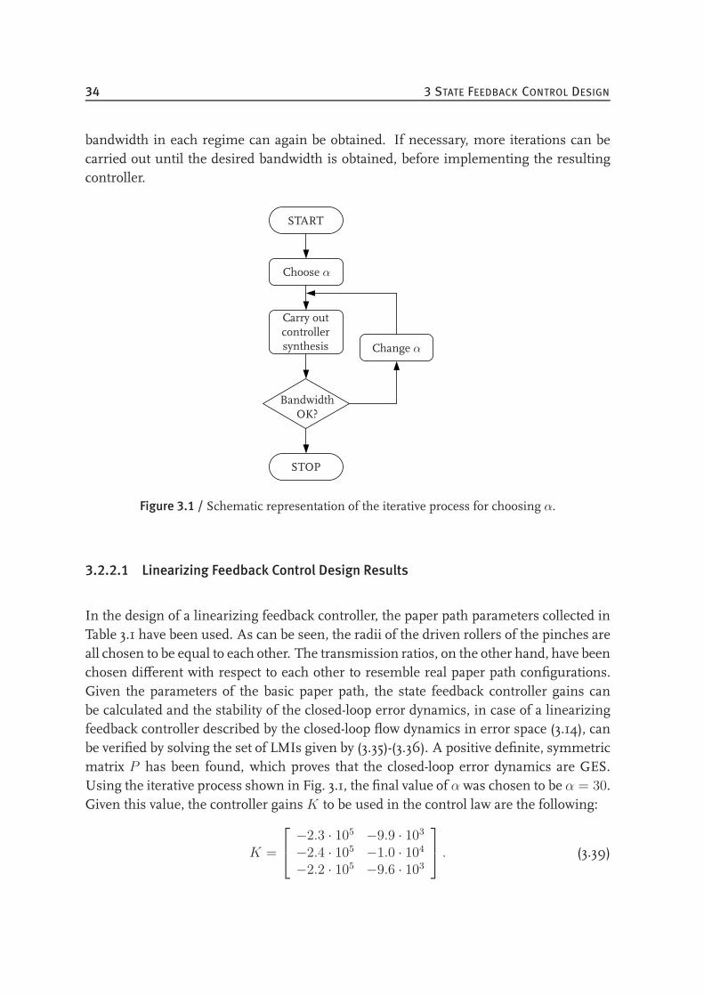
34 3 STATE FEEDBACK CONTROL DESIGN
bandwidth in each regime can again be obtained. If necessary, more iterations can becarried out until the desired bandwidth is obtained, before implementing the resultingcontroller.
START
Choose α
Carry outcontrollersynthesis
BandwidthOK?
STOP
Change α
Figure 3.1 / Schematic representation of the iterative process for choosing α.
3.2.2.1 Linearizing Feedback Control Design Results
In the design of a linearizing feedback controller, the paper path parameters collected inTable 3.1 have been used. As can be seen, the radii of the driven rollers of the pinches areall chosen to be equal to each other. The transmission ratios, on the other hand, have beenchosen different with respect to each other to resemble real paper path configurations.Given the parameters of the basic paper path, the state feedback controller gains canbe calculated and the stability of the closed-loop error dynamics, in case of a linearizingfeedback controller described by the closed-loop flow dynamics in error space (3.14), canbe verified by solving the set of LMIs given by (3.35)-(3.36). A positive definite, symmetricmatrix P has been found, which proves that the closed-loop error dynamics are GES.Using the iterative process shown in Fig. 3.1, the final value of α was chosen to be α = 30.Given this value, the controller gainsK to be used in the control law are the following:
K =
−2.3 · 105 −9.9 · 103
−2.4 · 105 −1.0 · 104
−2.2 · 105 −9.6 · 103
. (3.39)

3.2 NOMINAL SHEET FEEDBACK CONTROL DESIGN 35
Substitution of K(2, 1) and K(1, 1) into (3.38) shows that s2 = B1(1)B2(2)
= K(2,1)K(1,1)
. Since
also K(2,2)K(1,2)
= s2 and s3 = B1(1)B3(3)
= K(3,1)K(1,1)
= K(3,2)K(1,2)
, with s3 the scaling factor for thethird subsystem, we can conclude that the feedback controller completely linearizes thesystem, as expected.
Parameter Nominal Value
n1 18/37n2 14/30n3 15/30rP1 14 · 10−3 mrP2 14 · 10−3 mrP3 14 · 10−3 m
Table 3.1 / Paper path parameters for the nominal control design.
3.2.2.2 Partially Linearizing Feedback Control Design Results
The control design of a partially linearizing feedback controller has also been carried outusing the paper path parameters listed in Table 3.1. Given these parameters, the controllergains have been calculated using the approach presented in Section 3.2.1.2.
Focussing first on subsystem 1, the controller parameters for this subsystem have beencalculated using (3.37), after solving (3.35) and (3.36) with X = X1 and Y = Y1. Inthe calculation of these controller gains, the iterative process shown in Fig. 3.1 has beenused to check whether the desired bandwidth has been realized for the first subsystem.Choosing α = 40 resulted in K(1, 1) = −2.3 · 105 and K(1, 2) = −8.6 · 103. For thecalculation of K(2, 2) and K(2, 3), the range of values for these gains has been chosensuch that K(2, 2) = s2K(1, 2) ± 5 · 102 and K(3, 2) = s3K(1, 2) ± 5 · 102, respectively.In each of these ranges, several values of K(2, 2) and K(3, 2) satisfy (3.22) and (3.23) fori = 2 and i = 3, respectively. For illustration purposes, K(2, 2) and K(3, 2) were chosensuch that the largest difference with s2K(1, 2) and s3K(1, 2) was obtained, in order toobtain the largest discontinuity in es. This resulted in the following controller gainsK tobe used in the control law:
K =
−2.3 · 105 −8.6 · 103
−2.3 · 105 −9.5 · 103
−2.2 · 105 −8.9 · 103
. (3.40)
Substitution of K(2, 2) and K(1, 2) into (3.38) shows that K(2,2)K(1,2)
6= s2. Similarly, it can
be seen that K(3,2)K(1,2)
6= s3, which shows that the resulting controller does indeed not com-pletely linearize the system.
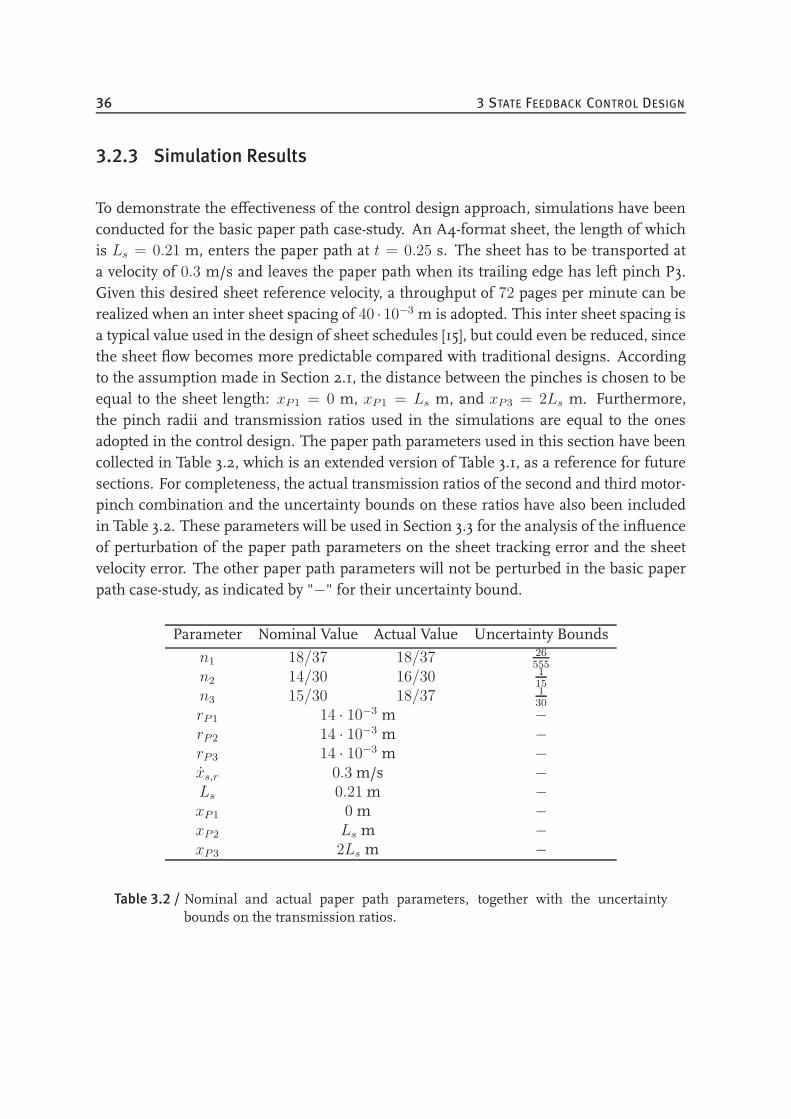
36 3 STATE FEEDBACK CONTROL DESIGN
3.2.3 Simulation Results
To demonstrate the effectiveness of the control design approach, simulations have beenconducted for the basic paper path case-study. An A4-format sheet, the length of whichis Ls = 0.21 m, enters the paper path at t = 0.25 s. The sheet has to be transported ata velocity of 0.3 m/s and leaves the paper path when its trailing edge has left pinch P3.Given this desired sheet reference velocity, a throughput of 72 pages per minute can berealized when an inter sheet spacing of 40 · 10−3 m is adopted. This inter sheet spacing isa typical value used in the design of sheet schedules [15], but could even be reduced, sincethe sheet flow becomes more predictable compared with traditional designs. Accordingto the assumption made in Section 2.1, the distance between the pinches is chosen to beequal to the sheet length: xP1 = 0 m, xP1 = Ls m, and xP3 = 2Ls m. Furthermore,the pinch radii and transmission ratios used in the simulations are equal to the onesadopted in the control design. The paper path parameters used in this section have beencollected in Table 3.2, which is an extended version of Table 3.1, as a reference for futuresections. For completeness, the actual transmission ratios of the second and third motor-pinch combination and the uncertainty bounds on these ratios have also been includedin Table 3.2. These parameters will be used in Section 3.3 for the analysis of the influenceof perturbation of the paper path parameters on the sheet tracking error and the sheetvelocity error. The other paper path parameters will not be perturbed in the basic paperpath case-study, as indicated by "−" for their uncertainty bound.
Parameter Nominal Value Actual Value Uncertainty Bounds
n1 18/37 18/37 26555
n2 14/30 16/30 115
n3 15/30 18/37 130
rP1 14 · 10−3 m −rP2 14 · 10−3 m −rP3 14 · 10−3 m −xs,r 0.3 m/s −Ls 0.21 m −xP1 0 m −xP2 Ls m −xP3 2Ls m −
Table 3.2 / Nominal and actual paper path parameters, together with the uncertaintybounds on the transmission ratios.
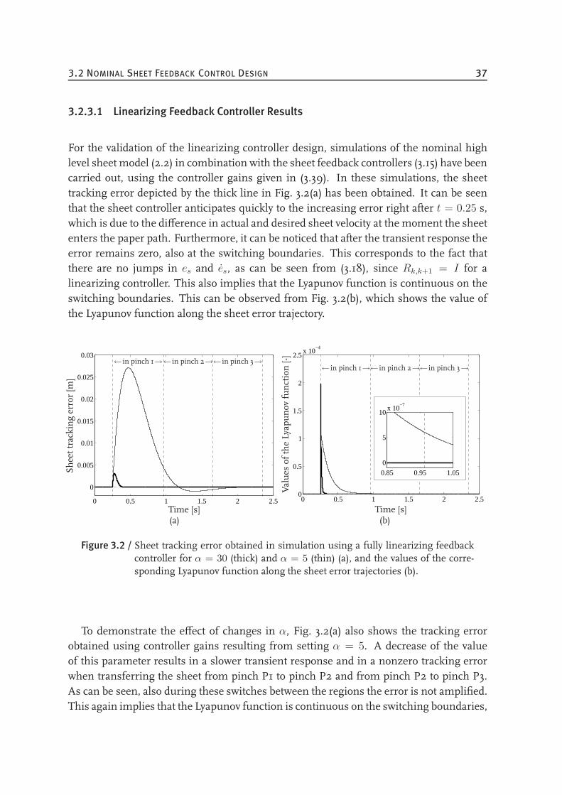
3.2 NOMINAL SHEET FEEDBACK CONTROL DESIGN 37
3.2.3.1 Linearizing Feedback Controller Results
For the validation of the linearizing controller design, simulations of the nominal highlevel sheet model (2.2) in combination with the sheet feedback controllers (3.15) have beencarried out, using the controller gains given in (3.39). In these simulations, the sheettracking error depicted by the thick line in Fig. 3.2(a) has been obtained. It can be seenthat the sheet controller anticipates quickly to the increasing error right after t = 0.25 s,which is due to the difference in actual and desired sheet velocity at the moment the sheetenters the paper path. Furthermore, it can be noticed that after the transient response theerror remains zero, also at the switching boundaries. This corresponds to the fact thatthere are no jumps in es and es, as can be seen from (3.18), since Rk,k+1 = I for alinearizing controller. This also implies that the Lyapunov function is continuous on theswitching boundaries. This can be observed from Fig. 3.2(b), which shows the value ofthe Lyapunov function along the sheet error trajectory.
0 0.5 1 1.5 2 2.5
0
0.005
0.01
0.015
0.02
0.025
0.03
Time [s]
Sheettrackingerror[m
]
← in pinch 1→← in pinch 2→← in pinch 3→
(a)
0 0.5 1 1.5 2 2.50
0.5
1
1.5
2
2.5x 10
−4
0.85 0.95 1.05
0
5
10x 10
−7
Time [s]
Values
oftheLyapunov
function[-]
← in pinch 1→← in pinch 2→← in pinch 3→
(b)
Figure 3.2 / Sheet tracking error obtained in simulation using a fully linearizing feedbackcontroller for α = 30 (thick) and α = 5 (thin) (a), and the values of the corre-sponding Lyapunov function along the sheet error trajectories (b).
To demonstrate the effect of changes in α, Fig. 3.2(a) also shows the tracking errorobtained using controller gains resulting from setting α = 5. A decrease of the valueof this parameter results in a slower transient response and in a nonzero tracking errorwhen transferring the sheet from pinch P1 to pinch P2 and from pinch P2 to pinch P3.As can be seen, also during these switches between the regions the error is not amplified.This again implies that the Lyapunov function is continuous on the switching boundaries,
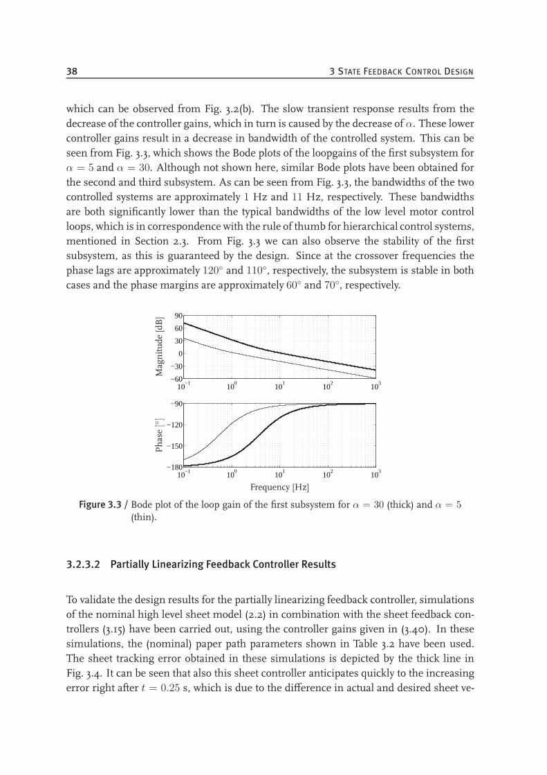
38 3 STATE FEEDBACK CONTROL DESIGN
which can be observed from Fig. 3.2(b). The slow transient response results from thedecrease of the controller gains, which in turn is caused by the decrease of α. These lowercontroller gains result in a decrease in bandwidth of the controlled system. This can beseen from Fig. 3.3, which shows the Bode plots of the loopgains of the first subsystem forα = 5 and α = 30. Although not shown here, similar Bode plots have been obtained forthe second and third subsystem. As can be seen from Fig. 3.3, the bandwidths of the twocontrolled systems are approximately 1 Hz and 11 Hz, respectively. These bandwidthsare both significantly lower than the typical bandwidths of the low level motor controlloops, which is in correspondence with the rule of thumb for hierarchical control systems,mentioned in Section 2.3. From Fig. 3.3 we can also observe the stability of the firstsubsystem, as this is guaranteed by the design. Since at the crossover frequencies thephase lags are approximately 120 and 110, respectively, the subsystem is stable in bothcases and the phase margins are approximately 60 and 70, respectively.
10−1
100
101
102
103
−60
−30
0
30
60
90
10−1
100
101
102
103
−180
−150
−120
−90
Magnitude
[dB]
Phase
[]
Frequency [Hz]
Figure 3.3 / Bode plot of the loop gain of the first subsystem for α = 30 (thick) and α = 5(thin).
3.2.3.2 Partially Linearizing Feedback Controller Results
To validate the design results for the partially linearizing feedback controller, simulationsof the nominal high level sheet model (2.2) in combination with the sheet feedback con-trollers (3.15) have been carried out, using the controller gains given in (3.40). In thesesimulations, the (nominal) paper path parameters shown in Table 3.2 have been used.The sheet tracking error obtained in these simulations is depicted by the thick line inFig. 3.4. It can be seen that also this sheet controller anticipates quickly to the increasingerror right after t = 0.25 s, which is due to the difference in actual and desired sheet ve-
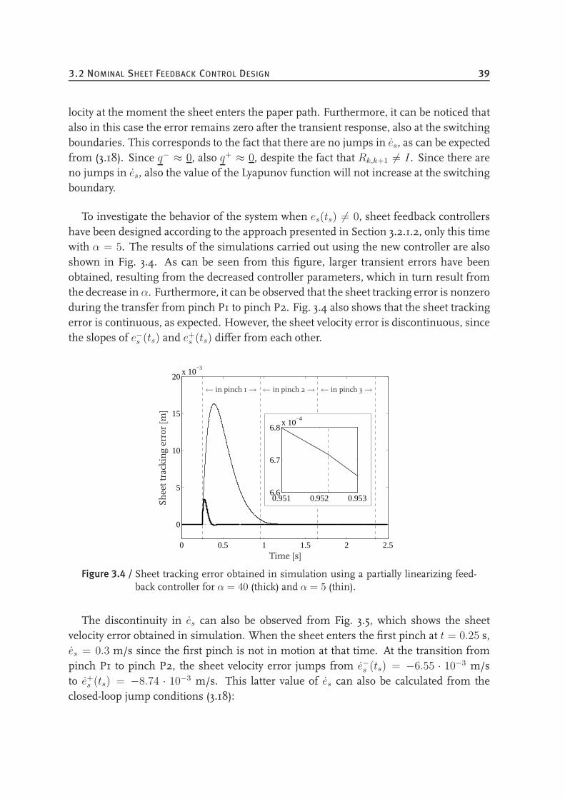
3.2 NOMINAL SHEET FEEDBACK CONTROL DESIGN 39
locity at the moment the sheet enters the paper path. Furthermore, it can be noticed thatalso in this case the error remains zero after the transient response, also at the switchingboundaries. This corresponds to the fact that there are no jumps in es, as can be expectedfrom (3.18). Since q− ≈ 0, also q+ ≈ 0, despite the fact that Rk,k+1 6= I . Since there areno jumps in es, also the value of the Lyapunov function will not increase at the switchingboundary.
To investigate the behavior of the system when es(ts) 6= 0, sheet feedback controllershave been designed according to the approach presented in Section 3.2.1.2, only this timewith α = 5. The results of the simulations carried out using the new controller are alsoshown in Fig. 3.4. As can be seen from this figure, larger transient errors have beenobtained, resulting from the decreased controller parameters, which in turn result fromthe decrease in α. Furthermore, it can be observed that the sheet tracking error is nonzeroduring the transfer from pinch P1 to pinch P2. Fig. 3.4 also shows that the sheet trackingerror is continuous, as expected. However, the sheet velocity error is discontinuous, sincethe slopes of e−s (ts) and e+s (ts) differ from each other.
0 0.5 1 1.5 2 2.5
0
5
10
15
20x 10
−3
0.951 0.952 0.9536.6
6.7
6.8x 10
−4
Time [s]
Sheettrackingerror[m
]
← in pinch 1→ ← in pinch 2→ ← in pinch 3→
Figure 3.4 / Sheet tracking error obtained in simulation using a partially linearizing feed-back controller for α = 40 (thick) and α = 5 (thin).
The discontinuity in es can also be observed from Fig. 3.5, which shows the sheetvelocity error obtained in simulation. When the sheet enters the first pinch at t = 0.25 s,es = 0.3 m/s since the first pinch is not in motion at that time. At the transition frompinch P1 to pinch P2, the sheet velocity error jumps from e−s (ts) = −6.55 · 10−3 m/sto e+s (ts) = −8.74 · 10−3 m/s. This latter value of es can also be calculated from theclosed-loop jump conditions (3.18):
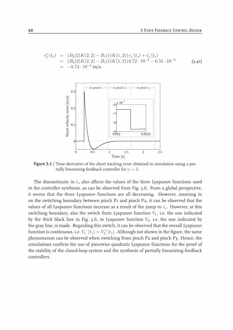
40 3 STATE FEEDBACK CONTROL DESIGN
e+s (ts) = (B2(2)K(2, 2) −B1(1)K(1, 2)) e−s (ts) + e−s (ts)= (B2(2)K(2, 2) −B1(1)K(1, 2)) 6.72 · 10−4 − 6.55 · 10−3
= −8.74 · 10−3 m/s.(3.41)
0 0.5 1 1.5 2 2.5
0
0.1
0.2
0.3
0.952 0.9525−9
−8
−7
−6x 10
−3
Time [s]
Sheetvelocityerror[m
/s]
← in pinch 1→ ← in pinch 2→ ← in pinch 3→
Figure 3.5 / Time derivative of the sheet tracking error obtained in simulation using a par-tially linearizing feedback controller for α = 5.
The discontinuity in es also affects the values of the three Lyapunov functions usedin the controller synthesis, as can be observed from Fig. 3.6. From a global perspective,it seems that the three Lyapunov functions are all decreasing. However, zooming inon the switching boundary between pinch P1 and pinch P2, it can be observed that thevalues of all Lyapunov functions increase as a result of the jump in es. However, at thisswitching boundary, also the switch from Lyapunov function V1, i.e. the one indicatedby the thick black line in Fig. 3.6, to Lyapunov function V2, i.e. the one indicated bythe gray line, is made. Regarding this switch, it can be observed that the overall Lyapunovfunction is continuous, i.e. V −1 (ts) = V +
2 (ts). Although not shown in the figure, the samephenomenon can be observed when switching from pinch P2 and pinch P3. Hence, thesimulations confirm the use of piecewise quadratic Lyapunov functions for the proof ofthe stability of the closed-loop system and the synthesis of partially linearizing feedbackcontrollers.
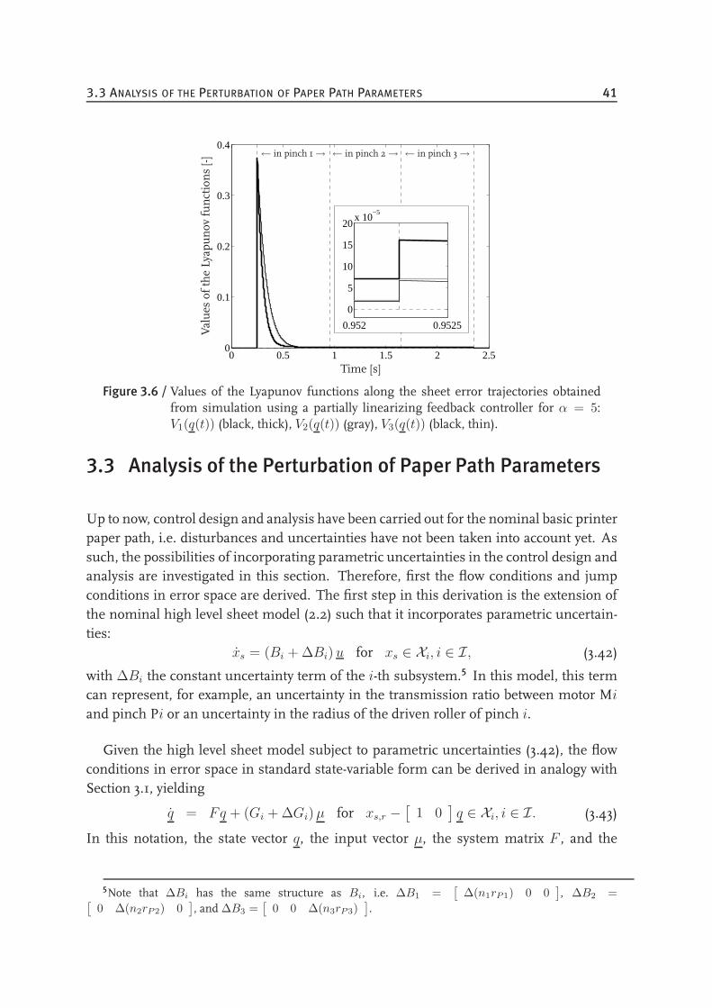
3.3 ANALYSIS OF THE PERTURBATION OF PAPER PATH PARAMETERS 41
0 0.5 1 1.5 2 2.50
0.1
0.2
0.3
0.4
0.952 0.9525
0
5
10
15
20x 10
−5
Time [s]
Values
oftheLyapunov
functions[-]
← in pinch 1→ ← in pinch 2→ ← in pinch 3→
Figure 3.6 / Values of the Lyapunov functions along the sheet error trajectories obtainedfrom simulation using a partially linearizing feedback controller for α = 5:V1(q(t)) (black, thick), V2(q(t)) (gray), V3(q(t)) (black, thin).
3.3 Analysis of the Perturbation of Paper Path Parameters
Up to now, control design and analysis have been carried out for the nominal basic printerpaper path, i.e. disturbances and uncertainties have not been taken into account yet. Assuch, the possibilities of incorporating parametric uncertainties in the control design andanalysis are investigated in this section. Therefore, first the flow conditions and jumpconditions in error space are derived. The first step in this derivation is the extension ofthe nominal high level sheet model (2.2) such that it incorporates parametric uncertain-ties:
xs = (Bi + ∆Bi) u for xs ∈ Xi, i ∈ I, (3.42)
with ∆Bi the constant uncertainty term of the i-th subsystem.5 In this model, this termcan represent, for example, an uncertainty in the transmission ratio between motor Miand pinch Pi or an uncertainty in the radius of the driven roller of pinch i.
Given the high level sheet model subject to parametric uncertainties (3.42), the flowconditions in error space in standard state-variable form can be derived in analogy withSection 3.1, yielding
q = Fq + (Gi + ∆Gi)µ for xs,r −[
1 0]q ∈ Xi, i ∈ I. (3.43)
In this notation, the state vector q, the input vector µ, the system matrix F , and the
5Note that ∆Bi has the same structure as Bi, i.e. ∆B1 =[
∆(n1rP1) 0 0], ∆B2 =[
0 ∆(n2rP2) 0], and ∆B3 =
[0 0 ∆(n3rP3)
].
42 3 STATE FEEDBACK CONTROL DESIGN
nominal input matrices Gi are defined as in Section 3.1. The uncertainty terms of the
input matrices are defined as ∆Gi =[
0 − (∆Bi)T
]T.
Similar to the flow conditions, also the jump conditions of the error dynamics can bederived in analogy with Section 3.1, yielding
q+(ts) =
[1 00 1
]q−(ts) +
[0T
Bk + ∆Bk − Bk+1 − ∆Bk+1
]u(ts), k ∈ K. (3.44)
Hence, the complete model of the uncertain open-loop sheet dynamics in error space isgiven by the flow conditions (3.43) and the jump conditions (3.44).
As in Section 3.2.1, the goal is to control the error dynamics using a state feedbackcontrol law (3.13). Using, this control law, the closed-loop flow dynamics in error spacecan be derived:
q = (F − (Gi + ∆Gi)K) q for(xs,r −
[1 0
]q)∈ Xi, i ∈ I. (3.45)
When we consider the transition from regime k to regime k + 1, the closed-loop jumpconditions can be derived from the open-loop jump conditions (3.44) in combination withthe control law ui (3.15), yielding
q+(ts) =
1 0
(Bk+1(k + 1) + ∆Bk+1(k + 1))K(k + 1, 2)−− (Bk(k) + ∆Bk(k))K(k, 2)
1
q−(ts)+
+
0
(Bk+1(k + 1) + ∆Bk+1(k + 1))K(k + 1, 1)−− (Bk(k) + ∆Bk(k))K(k, 1)
∫ ts
t0es(τ)dτ, k ∈ K.
(3.46)
For q = 0 to be the desired equilibrium point of the closed-loop error dynam-ics, the second term of (3.46) should be equal to 0. In analogy with Section 3.2.1,we know that enforcing (Bk+1(k + 1) + ∆Bk+1(k + 1))K(k + 1, 1) to be equal to(Bk(k) + ∆Bk(k))K(k, 1) would result in q = 0 to be the desired equilibrium point.However, since the actual values of the uncertainty matrices ∆Bk are assumed to be un-known, the feedback controllers (3.15) cannot fully or partially linearize the system for alluncertainties. Therefore, q = 0 is not an equilibrium point of the system and we cannot syn-
thesize a stabilizing controller for the uncertain error dynamics using the approach presented
in Section 3.2.1. Hence, instead of carrying out robust control design, the focus in theremainder of this section is on analysis. More specifically, given bounds on the uncer-tainties present in the paper path, the goal is to derive expressions for predicting theinfluence of these uncertainties on the magnitude of the jumps in es. Moreover, based onthe resulting expressions, the effect of these jumps on the evolution of the sheet trackingerror will be investigated, with the goal to be able to analytically predict this evolution and
3.3 ANALYSIS OF THE PERTURBATION OF PAPER PATH PARAMETERS 43
the maximum error value, and, hence, to be able to evaluate the system’s performanceanalytically.
3.3.1 Influence of Parameter Perturbations
In this section, first the influence of the parametric uncertainties on the jumps in es isanalyzed. Hence, the goal is to derive an expression for e+s (ts) as a function of theseuncertainties, the input matrices of the high level sheet flow model, and the controllerparameters. To realize this goal, we start from the relation for e+s (ts) in (3.46):6
e+s (ts) = ((Bk+1 + ∆Bk+1)K(k + 1, 2) − (Bk + ∆Bk)K(k, 2)) e−s (ts) + e−s (ts)+
+ ((Bk+1 + ∆Bk+1)K(k + 1, 1) − (Bk + ∆Bk)K(k, 1))
∫ ts
t0
es(τ)dτ︸ ︷︷ ︸
ck
,
k ∈ K.(3.47)
To express e+s (ts) as a function of the uncertainties, the input matrices, and the controllerparameters, the next step is to rewrite the unknown integral term in ck in (3.47). In doingthis, we calculate x−s (ts) in the k-th subsystem of the high level sheet flow model (3.42),with the control law substituted, given the initial condition u(t0) = 0:
x−s (ts) = − (Bk + ∆Bk)K(k, 1)
∫ ts
t0
es(τ)dτ−(Bk + ∆Bk)K(k, 2)e−s (ts), k ∈ K. (3.48)
Rewriting (3.48) yields the desired expression for the integral term:
∫ ts
t0
es(τ)dτ =−x−s (ts) − (Bk + ∆Bk)K(k, 2)e−s (ts)
(Bk + ∆Bk)K(k, 1), k ∈ K. (3.49)
With this expression, ck in (3.47) can be written as follows
ck =(−(Bk+1+∆Bk+1)K(k+1,1)
(Bk+∆Bk)K(k,1)+ 1
)(x−s (ts) + (Bk + ∆Bk)K(k, 2)e−s (ts)) ,
k ∈ K.(3.50)
If we now adopt the linearizing or partially linearizing controllers designed in Sec-tion 3.2.1, we know that
K(k, 1) =Bk+1
Bk
K(k + 1, 1), k ∈ K. (3.51)
6To simplify the notation, in the remainder of this section Bk(k), Bk+1(k+1), ∆Bk(k), and ∆Bk+1(k+1) have been replaced by Bk, Bk+1, ∆Bk, and ∆Bk+1, respectively.
44 3 STATE FEEDBACK CONTROL DESIGN
Substitution of this relation into (3.50) yields the following expression for ck:
ck =
(−(Bk+1+∆Bk+1)K(k+1,1)
(Bk+∆Bk)Bk+1
BkK(k+1,1)
+ 1
)(x−s (ts) + (Bk + ∆Bk)K(k, 2)e−s (ts)) ,
=(−Bk∆Bk+1+Bk+1∆Bk
Bk+1(Bk+∆Bk)
)(x−s (ts) + (Bk + ∆Bk)K(k, 2)e−s (ts)) , k ∈ K.
(3.52)
With this expression for ck, the desired relation between e+s (ts) and the uncertainties,the input matrices of the high level sheet flow model, and the controller parameters nowbecomes:
e+s (ts) = ((Bk+1 + ∆Bk+1)K(k + 1, 2) − (Bk + ∆Bk)K(k, 2)) e−s (ts) + e−s (ts)+(−Bk∆Bk+1+Bk+1∆Bk
Bk+1(Bk+∆Bk)
)(x−s (ts) + (Bk + ∆Bk)K(k, 2)e−s (ts)) , k ∈ K.
(3.53)
From (3.47) it can be observed that for the prediction of the jump in es, the sheettracking error and its time derivative right before switching are required, together with theactual sheet velocity at this time instant. Since these are in general not known beforehand,the desired prediction cannot be made. However, from the simulation results presentedin Section 3.2.3 it could be observed that with the sheet controllers calculated using thelarge values of α, i.e. α = 30 and α = 40, and with a sheet reference velocity of 0.3 m/s,a zero tracking error and a zero velocity error could be realized at ts with both the fullyand the partially linearizing feedback controller. If we assume that in case parameteruncertainties are present in the paper path, e−s (ts) = 0 and e−s (ts) = 0 can also be realized,a significant simplification of (3.53) can be obtained. Since under these assumptionsx−s (ts) = xs,r, e+s (ts) can be expressed as a function of the uncertainties and the inputmatrices of the high level sheet flow model:
e+s (ts) =(−Bk∆Bk+1+Bk+1∆Bk
Bk+1(Bk+∆Bk)
)xs,r, k ∈ K. (3.54)
As can be seen from (3.54), the jump in es is in this case only a function of the nom-inal system parameters, the uncertainty terms, and the sheet reference velocity. Morespecifically, in the case of fully or partially linearizing feedback controllers, the controller gains
do not influence the jump in es, since this jump is fully determined by the system parameters.Since the nominal system parameters and the sheet reference velocity are assumed tobe known, (3.54) can be evaluated for various values of the uncertainty terms within theupper and lower bounds on these terms. This way, insight is obtained in the influenceof various combinations of the uncertainty terms on the value of the jump in es. One ofthese combinations can already easily be obtained from (3.54): if there are no uncertain-ties present, there will be no jumps in es on the transitions between two regimes, whichcoincides with the closed-loop jump conditions (3.46).
Once the jump in es can be predicted, this prediction can be used to evaluate the effecton the sheet tracking error. For analysis purposes, we consider the transition from regime
3.3 ANALYSIS OF THE PERTURBATION OF PAPER PATH PARAMETERS 45
k to regime k + 1, assuming the sheet is not forced back into the previous pinch, i.e. noimmediate switching back to the previous regime occurs. Since the states of the errordynamics are both assumed to be equal to zero just before the transition occurs, q+(ts) =[e+s (ts) e+s (ts)
]Tcan be considered as an initial condition of the flow dynamics active
in regime k + 1, with e+s (ts) = 0 since e+s (ts) = e−s (ts) and with e+s (ts) calculated fromin (3.54). By solving the set of differential equations in (3.45), the evolution of the sheettracking error can be predicted as a function of time. Via this approach, also the evolutionof the sheet tracking error in the first regime can be predicted. Given the second orderdynamics active in each regime of the closed-loop system (3.45), it is plausible to assumethat each subsystem has two complex eigenvalues λi1,2
= σi ± jωi, as a result of whichthe general solution of the set of differential equations for each subsystem is given by:
ei(t) = Ci,1eσit cos(ωit) + Ci,2e
σit sin(ωit), i ∈ I, (3.55)
with the constants Ci,1 and Ci,2 calculated from the initial conditions, leading to Ci,1 = 0,
Ci,2 = e+s (ts)ωi
, and therefore
ei(t) =e+s (ts)
ωieσit sin(ωit), i ∈ I. (3.56)
Hence, using (3.56) the evolution of the sheet tracking error can be predicted. To calculatethe maximum of minimum value of ei, its time derivative, given by
ei(t) =e+s (ts)
ωiσie
σit sin(ωit) +e+s (ts)
ωieσitωi cos(ωit), i ∈ I, (3.57)
is set equal to zero. Solving the resulting equality for t yields the time t⋆ at which thesheet tracking error has its maximum or minimum value:
t⋆ =− arctan
(ωi
σi
)
ωi, i ∈ I. (3.58)
Substitution of (3.58) into (3.56) yields the expression for calculating the maximum orminimum value of the tracking error in subsystem i:
ei(t⋆) =
e+s (ts)√σ2i + ω2
i
e− σi
ωiarctan
(ωiσi
)
, i ∈ I. (3.59)
With the derivation of (3.56) and (3.59), the evolution of the sheet tracking error and itsmaximum value can be predicted in case a zero tracking error and a zero velocity error arerealized just before a transition to a subsequent regime occurs. In the next subsection,simulation results will be presented to judge the quality of these predictions.
46 3 STATE FEEDBACK CONTROL DESIGN
3.3.2 Simulation Results
To analyze the behavior of the system subject to perturbations of the paper path param-eters and to validate if the jumps in es and the resulting maximum deviations of thesheet tracking error can be predicted correctly, simulations have been carried out usingtwo types of controllers: the ones that result in a nonzero tracking error and velocityerror right before switching and the ones that yield e−s (ts) = e−s (ts) ≈ 0. Initially, westart with the analysis of the results obtained using the latter type of sheet controllers.Hence, we make the assumption that the transient behavior in each regime, initiated bythe perturbation of the paper path parameters, has decayed before the transition to thenext regime occurs. Before presenting the simulation results, first (3.54) is evaluated forvarious uncertainties present in adjacent subsystems. The bounds on these uncertaintiesare quantified by introducing an additional transmission ratio of 16/30. Since this ratio islarger than the nominal ratios listed in Table 3.2, the maximum possible variations of theratios, which will take the role of uncertainty bounds upon the nominal ratios, can be cal-culated. Given these uncertainty bounds, also listed in Table 3.2, (3.54) can be evaluatedfor various uncertainties within these bounds. The results of this evaluation are shownin Fig. 3.7. From Fig. 3.7(a), which shows the jump in es as a function of ∆B1 and ∆B2,it can be seen that for fixed values of ∆B1, the jump in es varies linearly with changingvalues of ∆B2, as can be expected from (3.54). When considering fixed values of ∆B2, itcan be observed that the jump in es increases nonlinearly with increasing values of ∆B1.Given the ranges of uncertainty terms ∆B1 and ∆B2, no large jumps in es are predicted.Hence, the increase in tracking error after the transition from regime 1 to regime 2 dueto the perturbations of the transmission ratios will be limited, as can be seen from (3.59).From Fig. 3.7(b), which shows the jump in es as a function of ∆B2 and ∆B3, similarconclusions can be drawn: for fixed values of ∆B2, the jump in es varies linearly withchanging values of ∆B3, whereas fixing the values of ∆B3 results in jumps in es thatincrease nonlinearly with an increasing ∆B2. Also in this case, relatively small jumps ines, and therefore small increases in es after the transition will be obtained.
In the simulations that have been carried out, the actual paper path parameters listedin Table 3.2 have been used. Hence, the actual gains of the second and third subsystemvary 14% and −3% with respect to their nominal values, respectively. As an example,the fully linearizing controller designed in Section 3.2.2.1, i.e. with the decay rate of theLyapunov function chosen to be α = 30, has been used. Although not discussed here,similar results have been obtained using partially linearizing controllers. The trackingerror obtained in simulation is depicted in Fig. 3.8. It can be seen that the tracking errorincreases in the negative direction right after the sheet enters the second pinch, whichcorresponds with the increased value of the second transmission ratio with respect to theone the feedback controller was designed for. On the other hand, a positive tracking error
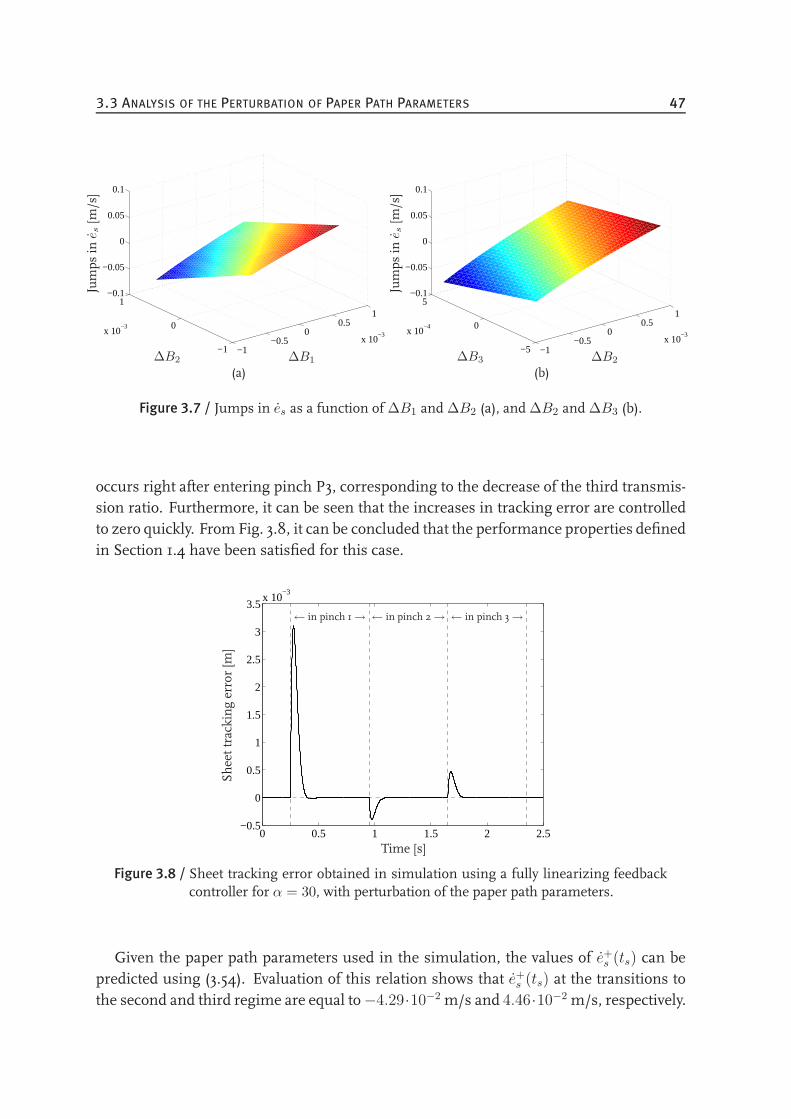
3.3 ANALYSIS OF THE PERTURBATION OF PAPER PATH PARAMETERS 47
−1−0.5
00.5
1
x 10−3
−1
0
1
x 10−3
−0.1
−0.05
0
0.05
0.1
∆B1∆B2
Jumps
ine
s[m
/s]
(a)
−1−0.5
00.5
1
x 10−3
−5
0
5
x 10−4
−0.1
−0.05
0
0.05
0.1
∆B2∆B3
Jumps
ine
s[m
/s]
(b)
Figure 3.7 / Jumps in es as a function of ∆B1 and ∆B2 (a), and ∆B2 and ∆B3 (b).
occurs right after entering pinch P3, corresponding to the decrease of the third transmis-sion ratio. Furthermore, it can be seen that the increases in tracking error are controlledto zero quickly. From Fig. 3.8, it can be concluded that the performance properties definedin Section 1.4 have been satisfied for this case.
0 0.5 1 1.5 2 2.5−0.5
0
0.5
1
1.5
2
2.5
3
3.5x 10
−3
Time [s]
Sheettrackingerror[m
]
← in pinch 1→ ← in pinch 2→ ← in pinch 3→
Figure 3.8 / Sheet tracking error obtained in simulation using a fully linearizing feedbackcontroller for α = 30, with perturbation of the paper path parameters.
Given the paper path parameters used in the simulation, the values of e+s (ts) can bepredicted using (3.54). Evaluation of this relation shows that e+s (ts) at the transitions tothe second and third regime are equal to−4.29·10−2 m/s and 4.46·10−2 m/s, respectively.
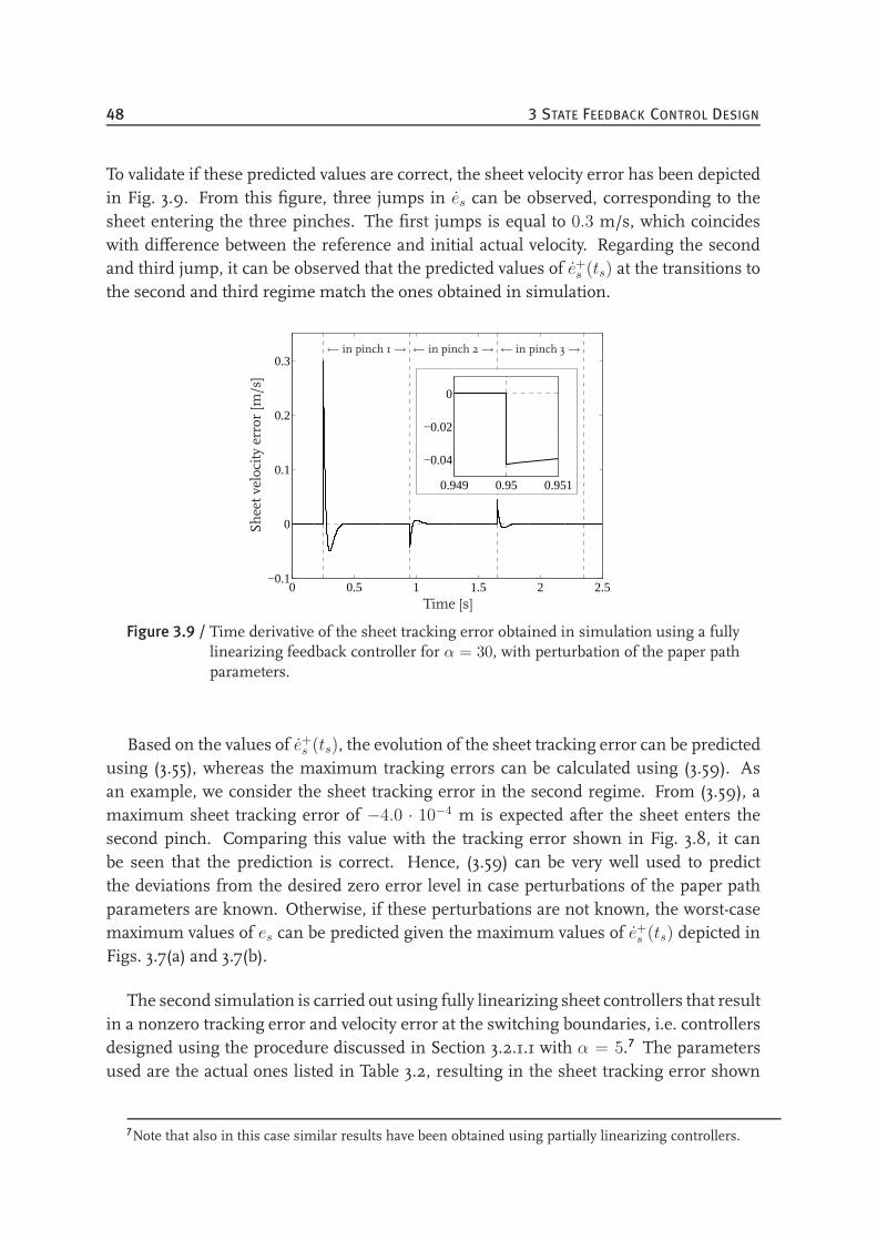
48 3 STATE FEEDBACK CONTROL DESIGN
To validate if these predicted values are correct, the sheet velocity error has been depictedin Fig. 3.9. From this figure, three jumps in es can be observed, corresponding to thesheet entering the three pinches. The first jumps is equal to 0.3 m/s, which coincideswith difference between the reference and initial actual velocity. Regarding the secondand third jump, it can be observed that the predicted values of e+s (ts) at the transitions tothe second and third regime match the ones obtained in simulation.
0 0.5 1 1.5 2 2.5−0.1
0
0.1
0.2
0.3
0.949 0.95 0.951
−0.04
−0.02
0
Time [s]
Sheetvelocityerror[m
/s]
← in pinch 1→ ← in pinch 2→ ← in pinch 3→
Figure 3.9 / Time derivative of the sheet tracking error obtained in simulation using a fullylinearizing feedback controller for α = 30, with perturbation of the paper pathparameters.
Based on the values of e+s (ts), the evolution of the sheet tracking error can be predictedusing (3.55), whereas the maximum tracking errors can be calculated using (3.59). Asan example, we consider the sheet tracking error in the second regime. From (3.59), amaximum sheet tracking error of −4.0 · 10−4 m is expected after the sheet enters thesecond pinch. Comparing this value with the tracking error shown in Fig. 3.8, it canbe seen that the prediction is correct. Hence, (3.59) can be very well used to predictthe deviations from the desired zero error level in case perturbations of the paper pathparameters are known. Otherwise, if these perturbations are not known, the worst-casemaximum values of es can be predicted given the maximum values of e+s (ts) depicted inFigs. 3.7(a) and 3.7(b).
The second simulation is carried out using fully linearizing sheet controllers that resultin a nonzero tracking error and velocity error at the switching boundaries, i.e. controllersdesigned using the procedure discussed in Section 3.2.1.1 with α = 5.7 The parametersused are the actual ones listed in Table 3.2, resulting in the sheet tracking error shown
7Note that also in this case similar results have been obtained using partially linearizing controllers.
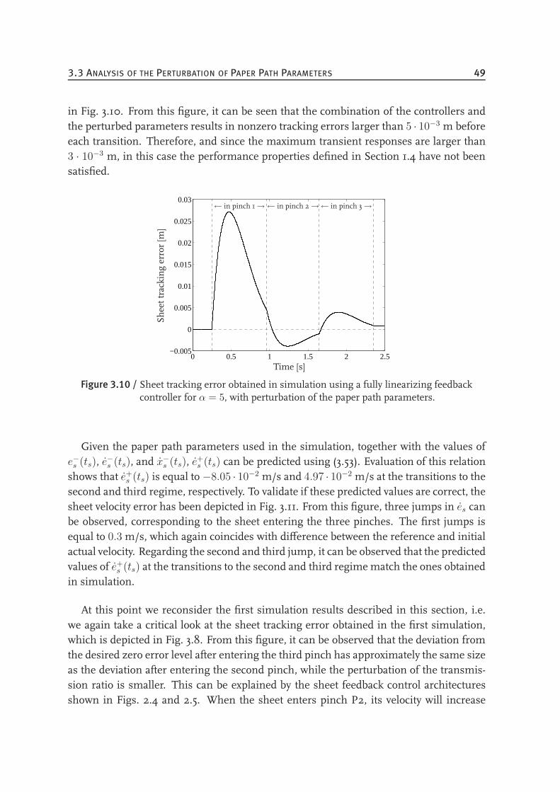
3.3 ANALYSIS OF THE PERTURBATION OF PAPER PATH PARAMETERS 49
in Fig. 3.10. From this figure, it can be seen that the combination of the controllers andthe perturbed parameters results in nonzero tracking errors larger than 5 · 10−3 m beforeeach transition. Therefore, and since the maximum transient responses are larger than3 · 10−3 m, in this case the performance properties defined in Section 1.4 have not beensatisfied.
0 0.5 1 1.5 2 2.5−0.005
0
0.005
0.01
0.015
0.02
0.025
0.03
Time [s]
Sheettrackingerror[m
]
← in pinch 1→← in pinch 2→← in pinch 3→
Figure 3.10 / Sheet tracking error obtained in simulation using a fully linearizing feedbackcontroller for α = 5, with perturbation of the paper path parameters.
Given the paper path parameters used in the simulation, together with the values ofe−s (ts), e−s (ts), and x−s (ts), e+s (ts) can be predicted using (3.53). Evaluation of this relationshows that e+s (ts) is equal to −8.05 · 10−2 m/s and 4.97 · 10−2 m/s at the transitions to thesecond and third regime, respectively. To validate if these predicted values are correct, thesheet velocity error has been depicted in Fig. 3.11. From this figure, three jumps in es canbe observed, corresponding to the sheet entering the three pinches. The first jumps isequal to 0.3 m/s, which again coincides with difference between the reference and initialactual velocity. Regarding the second and third jump, it can be observed that the predictedvalues of e+s (ts) at the transitions to the second and third regimematch the ones obtainedin simulation.
At this point we reconsider the first simulation results described in this section, i.e.we again take a critical look at the sheet tracking error obtained in the first simulation,which is depicted in Fig. 3.8. From this figure, it can be observed that the deviation fromthe desired zero error level after entering the third pinch has approximately the same sizeas the deviation after entering the second pinch, while the perturbation of the transmis-sion ratio is smaller. This can be explained by the sheet feedback control architecturesshown in Figs. 2.4 and 2.5. When the sheet enters pinch P2, its velocity will increase
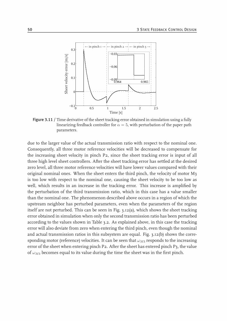
50 3 STATE FEEDBACK CONTROL DESIGN
0 0.5 1 1.5 2 2.5−0.1
0
0.1
0.2
0.3
0.964 0.965−0.09
−0.06
−0.03
Time [s]
Sheetvelocityerror[m
/s]
← in pinch 1→ ← in pinch 2→ ← in pinch 3→
Figure 3.11 / Time derivative of the sheet tracking error obtained in simulation using a fullylinearizing feedback controller for α = 5, with perturbation of the paper pathparameters.
due to the larger value of the actual transmission ratio with respect to the nominal one.Consequently, all three motor reference velocities will be decreased to compensate forthe increasing sheet velocity in pinch P2, since the sheet tracking error is input of allthree high level sheet controllers. After the sheet tracking error has settled at the desiredzero level, all three motor reference velocities will have lower values compared with theiroriginal nominal ones. When the sheet enters the third pinch, the velocity of motor M3is too low with respect to the nominal one, causing the sheet velocity to be too low aswell, which results in an increase in the tracking error. This increase is amplified bythe perturbation of the third transmission ratio, which in this case has a value smallerthan the nominal one. The phenomenon described above occurs in a region of which theupstream neighbor has perturbed parameters, even when the parameters of the regionitself are not perturbed. This can be seen in Fig. 3.12(a), which shows the sheet trackingerror obtained in simulation when only the second transmission ratio has been perturbedaccording to the values shown in Table 3.2. As explained above, in this case the trackingerror will also deviate from zero when entering the third pinch, even though the nominaland actual transmission ratios in this subsystem are equal. Fig. 3.12(b) shows the corre-sponding motor (reference) velocities. It can be seen that ωM3 responds to the increasingerror of the sheet when entering pinch P2. After the sheet has entered pinch P3, the valueof ωM3 becomes equal to its value during the time the sheet was in the first pinch.
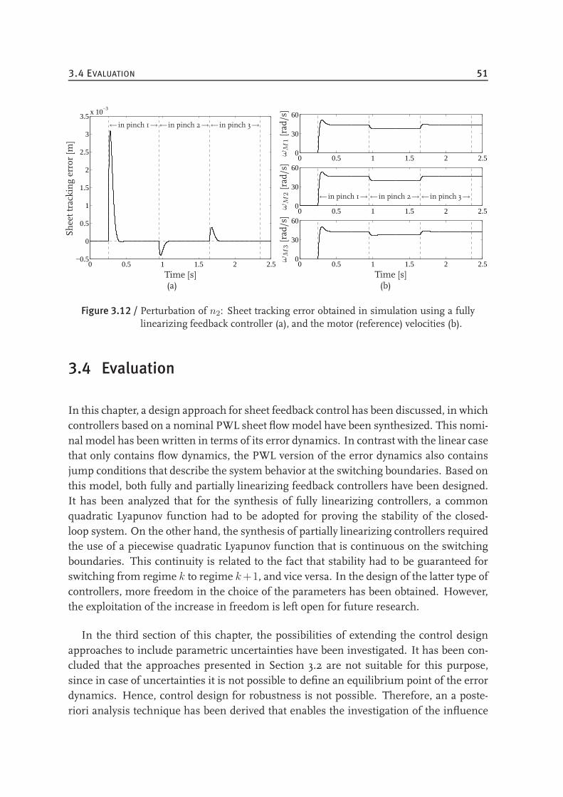
3.4 EVALUATION 51
0 0.5 1 1.5 2 2.5−0.5
0
0.5
1
1.5
2
2.5
3
3.5x 10
−3
Time [s]
Sheettrackingerror[m
]
← in pinch 1→← in pinch 2→← in pinch 3→
(a)
0 0.5 1 1.5 2 2.50
30
60
0 0.5 1 1.5 2 2.50
30
60
0 0.5 1 1.5 2 2.50
30
60
ωM
1[rad/s]
ωM
2[rad/s]
ωM
3[rad/s]
Time [s]
← in pinch 1→← in pinch 2→← in pinch 3→
(b)
Figure 3.12 / Perturbation of n2: Sheet tracking error obtained in simulation using a fullylinearizing feedback controller (a), and the motor (reference) velocities (b).
3.4 Evaluation
In this chapter, a design approach for sheet feedback control has been discussed, in whichcontrollers based on a nominal PWL sheet flowmodel have been synthesized. This nomi-nal model has been written in terms of its error dynamics. In contrast with the linear casethat only contains flow dynamics, the PWL version of the error dynamics also containsjump conditions that describe the system behavior at the switching boundaries. Based onthis model, both fully and partially linearizing feedback controllers have been designed.It has been analyzed that for the synthesis of fully linearizing controllers, a commonquadratic Lyapunov function had to be adopted for proving the stability of the closed-loop system. On the other hand, the synthesis of partially linearizing controllers requiredthe use of a piecewise quadratic Lyapunov function that is continuous on the switchingboundaries. This continuity is related to the fact that stability had to be guaranteed forswitching from regime k to regime k+1, and vice versa. In the design of the latter type ofcontrollers, more freedom in the choice of the parameters has been obtained. However,the exploitation of the increase in freedom is left open for future research.
In the third section of this chapter, the possibilities of extending the control designapproaches to include parametric uncertainties have been investigated. It has been con-cluded that the approaches presented in Section 3.2 are not suitable for this purpose,since in case of uncertainties it is not possible to define an equilibrium point of the errordynamics. Hence, control design for robustness is not possible. Therefore, an a poste-riori analysis technique has been derived that enables the investigation of the influence
52 3 STATE FEEDBACK CONTROL DESIGN
of parametric uncertainties on the tracking performance of the system. In this analysis,two cases have been distinguished. In the first case, the sheet tracking error and its timederivative are assumed to be zero right before the sheet enters the new pinch, i.e. thelinear subsystems are assumed to be fast enough to reach the steady state mode beforeswitching. In the second case, nonzero tracking errors at the switching boundaries areconsidered. In the first case, it has been assumed for analysis purposes that after enter-ing a new pinch, the sheet is not immediately forced back into the previous pinch, i.e. noimmediate switching back to the previous regime is allowed to occur. The simulationsshowed that the performance properties are still satisfied. However, as the uncertain-ties were not incorporated in the control design, no a priori guarantees on the systembehavior can be given from a control point of view. More specifically, the performanceguarantees should be obtained from the mechanical design of the system, as the jumpsin es are not influenced by the controller gains, but only by the paper path parameters.
In the control design approaches presented in this chapter, the structure of the sheetfeedback controllers solely depends on the order of the sheet reference profile that istaken into account in the derivation of the error dynamics. This implies that high orderprofiles lead to equally high order controllers. So far, only first order reference profileshave been considered, while in real printer paper paths piecewise linear velocity profilesare commonly used. Hence, a next step in sheet feedback control design using the ap-proach presented in this chapter is the extension to take into account more realistic sheetreference profiles. Another observation regarding the control design presented in thischapter is that no additional dynamics have been added to the controller. One could thinkof, for example, a high frequency roll-off to prevent the low level motor control loops tobe excited by high frequency components in the motor reference velocities that cannot betracked. A third observation is that the controller design is frequency independent, i.e.possible a priori knowledge on important frequency ranges, e.g. ranges in which distur-bances are likely to be present, is not taken into account in the design. Hence, an itemfor future research could be to incorporate additional dynamics in the design of the sheetfeedback controllers, while still using the design approach presented in this chapter.
Given the evaluation of the control design presented in this chapter, in the next chapteran alternative control design procedure will be presented for both the nominal and theuncertain high level sheet flow model. The main reasons for considering this alterna-tive are the possibility to carry out control design for robustness, the independency of thecontrol design and the controller structure with respect to the order of the sheet referenceprofiles, and the possibility to incorporate bandwidth requirements and possible a prioriknowledge on important frequency ranges. More specifically, in the alternative approach,disturbance attenuation properties can be incorporated into the design via frequency de-pendent weighting filters. Using this approach, controllers can be shaped according tothe designer’s demands.
CHAPTER FOUR
Output Feedback Control Design
4.1 The Tracking Control Problem . . . . . . . . . . . . . . . . . . . . . . . 53
4.2 Nominal Sheet Feedback Control Design . . . . . . . . . . . . . . . . . . 55
4.3 Robust Sheet Feedback Control Design . . . . . . . . . . . . . . . . . . . 66
4.4 Stability Analysis for Non-ideal Low Level Dynamics . . . . . . . . . . . 77
4.5 Evaluation . . . . . . . . . . . . . . . . . . . . . . . . . . . . . . . . . . . 78
4.1 The Tracking Control Problem
In this chapter, the second approach for sheet feedback control design for the basic paperpath case-study is presented. The goal of the control design procedure is the same asthe one in Chapter 3, i.e. the synthesis of sheet feedback controllers that make the sheetsin the paper path track a reference trajectory, satisfying the performance properties pre-sented in Section 1.4. In contradiction to Chapter 3, in which the influence of parametricuncertainties on the tracking performance of the system was considered via an a pos-teriori analysis technique, in this chapter the focus will eventually be on control designfor robustness. Hence, also in this chapter we will concentrate on feedback design only,leaving feedforward control design out of consideration.
As already shortly mentioned in Section 3.1, the focus in this chapter is on controldesign that guarantees performance in the H∞ sense. Known results from literature re-garding this topic can be found in [23, 57], in which state feedback control design forPWL systems is proposed. Given the control law, it is shown that upper bounds on theinduced L2-norm of the operator from the control input [57] or the disturbance input [23]
53
54 4 OUTPUT FEEDBACK CONTROL DESIGN
to the controlled output can be given. Based on the work presented in [23], extensionsfor controlling uncertain PWL systems via state feedback are presented in [11, 22]. Inthis chapter we will take an alternative approach. First of all, we will present a controllersynthesis technique that is based on output feedback. Secondly, we will make use of fre-quency domain weighting filters to shape the closed-loop dynamics in each regime of thePWL sheet flow model. Hence, the novelty of the controller synthesis that will be carriedout in this chapter is that linear H∞ output-based control design techniques [69] for thedynamics of each subsystem are combined with stability and performance requirementsfor the switched system. For carrying out the controller synthesis, LMI-based approachesfor linear systems known in literature, e.g. [29, 30, 67], are extended to the PWL case.More specifically, the stability and performance requirements for both the subsystems,incorporated via frequency dependent weighting filters, and the switched system, usingL2-gains, are combined into a joint optimization problem, enforcing both (robust) stabil-ity and (robust) performance of the subsystems and the closed-loop switched system.
As in Chapter 3, we will focus initially on sheet feedback control design based on thenominal sheet flow model (2.2), after which control design will be considered that guar-antees robust stability and robust performance of the closed-loop system. In this case,however, the output feedback controllers will based on the dynamics described by thePWL sheet flow model itself, instead of the sheet dynamics in error space. Hence, inthis approach the sheet reference profile is not taken into account and does thereforenot enforce the structure of the designed controllers, i.e. the resulting controllers are notnecessarily PI feedback controllers. By making use of the frequency domain weightingfilters for the dynamics in each region of the PWL sheet model, bandwidth requirementson the sheet control loop can be incorporated in the control design. Moreover, the influ-ence of disturbances can be penalized in frequency ranges in which they are present, anddesired properties of the controllers, e.g. integral action and high frequency roll-off, canbe enforced. Hence, in this way both performance and stability of the closed-loop systemin each region can be guaranteed.
Preliminary results of applying nominal H∞ control design to the paper path case-study are presented in [18]. In [18], the dynamics of the low level motor control loopswere taken into account in the design of the sheet feedback controllers. Consequently, thestability of the overall system could be guaranteed via the controller synthesis. However,the approach presented in [18] resulted in sheet feedback controllers of 24-th order. Sincein an embedded environment often no dedicated processors are available exclusively forreal-time motion control tasks, it is desirable to keep the controller order low to reducethe computational burden imposed by the sheet feedback control loops. Therefore, in thischapter controllers are initially designed based on the nominal PWL sheet flow dynamicsin which the controlledmotor dynamics are not taken into account, leading to lower ordersheet feedback controllers.
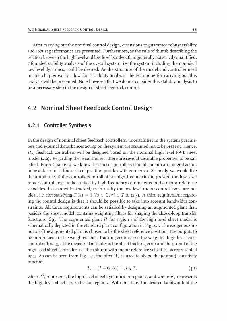
4.2 NOMINAL SHEET FEEDBACK CONTROL DESIGN 55
After carrying out the nominal control design, extensions to guarantee robust stabilityand robust performance are presented. Furthermore, as the rule of thumb describing therelation between the high level and low level bandwidth is generally not strictly quantified,a founded stability analysis of the overall system, i.e. the system including the non-ideallow level dynamics, could be desired. As the structure of the model and controller usedin this chapter easily allow for a stability analysis, the technique for carrying out thisanalysis will be presented. Note however, that we do not consider this stability analysis tobe a necessary step in the design of sheet feedback control.
4.2 Nominal Sheet Feedback Control Design
4.2.1 Controller Synthesis
In the design of nominal sheet feedback controllers, uncertainties in the system parame-ters and external disturbances acting on the system are assumed not to be present. Hence,H∞ feedback controllers will be designed based on the nominal high level PWL sheetmodel (2.2). Regarding these controllers, there are several desirable properties to be sat-isfied. From Chapter 3, we know that these controllers should contain an integral actionto be able to track linear sheet position profiles with zero error. Secondly, we would likethe amplitude of the controllers to roll-off at high frequencies to prevent the low levelmotor control loops to be excited by high frequency components in the motor referencevelocities that cannot be tracked, as in reality the low level motor control loops are notideal, i.e. not satisfying Ti(s) = 1, ∀s ∈ C, ∀i ∈ I in (2.3). A third requirement regard-ing the control design is that it should be possible to take into account bandwidth con-straints. All three requirements can be satisfied by designing an augmented plant that,besides the sheet model, contains weighting filters for shaping the closed-loop transferfunctions [69]. The augmented plant Pi for region i of the high level sheet model isschematically depicted in the standard plant configuration in Fig. 4.1. The exogenous in-put w of the augmented plant is chosen to be the sheet reference position. The outputs tobe minimized are the weighted sheet tracking error ze and the weighted high level sheetcontrol output zu. Themeasured output v is the sheet tracking error and the output of thehigh level sheet controller, i.e. the column with motor reference velocities, is representedby u. As can be seen from Fig. 4.1, the filterWe is used to shape the (output) sensitivityfunction
Si = (I +GiKi)−1 , i ∈ I, (4.1)
where Gi represents the high level sheet dynamics in region i, and where Ki representsthe high level sheet controller for region i. With this filter the desired bandwidth of the
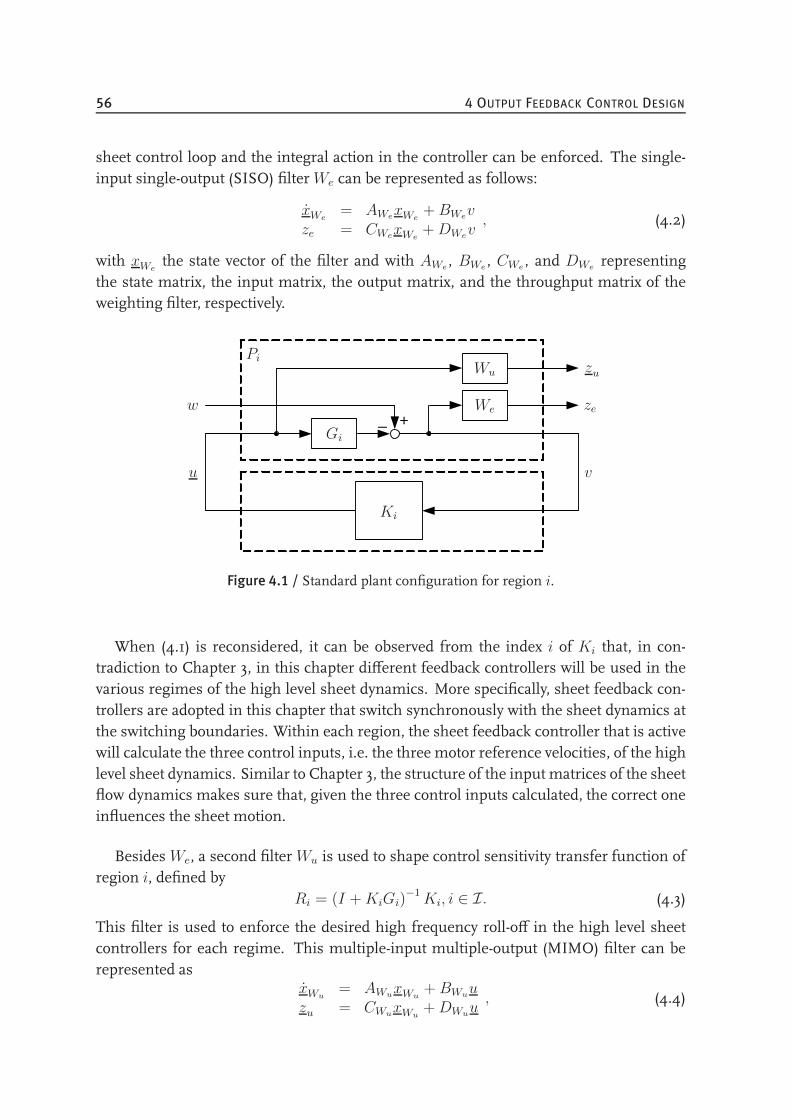
56 4 OUTPUT FEEDBACK CONTROL DESIGN
sheet control loop and the integral action in the controller can be enforced. The single-input single-output (SISO) filterWe can be represented as follows:
xWe= AWe
xWe+BWe
vze = CWe
xWe+DWe
v, (4.2)
with xWethe state vector of the filter and with AWe
, BWe, CWe
, and DWerepresenting
the state matrix, the input matrix, the output matrix, and the throughput matrix of theweighting filter, respectively.
_ +
Wu
We
Gi
Pi
Ki
w
u v
ze
zu
Figure 4.1 / Standard plant configuration for region i.
When (4.1) is reconsidered, it can be observed from the index i of Ki that, in con-tradiction to Chapter 3, in this chapter different feedback controllers will be used in thevarious regimes of the high level sheet dynamics. More specifically, sheet feedback con-trollers are adopted in this chapter that switch synchronously with the sheet dynamics atthe switching boundaries. Within each region, the sheet feedback controller that is activewill calculate the three control inputs, i.e. the three motor reference velocities, of the highlevel sheet dynamics. Similar to Chapter 3, the structure of the input matrices of the sheetflow dynamics makes sure that, given the three control inputs calculated, the correct oneinfluences the sheet motion.
BesidesWe, a second filterWu is used to shape control sensitivity transfer function ofregion i, defined by
Ri = (I +KiGi)−1Ki, i ∈ I. (4.3)
This filter is used to enforce the desired high frequency roll-off in the high level sheetcontrollers for each regime. This multiple-input multiple-output (MIMO) filter can berepresented as
xWu= AWu
xWu+BWu
uzu = CWu
xWu+DWu
u, (4.4)
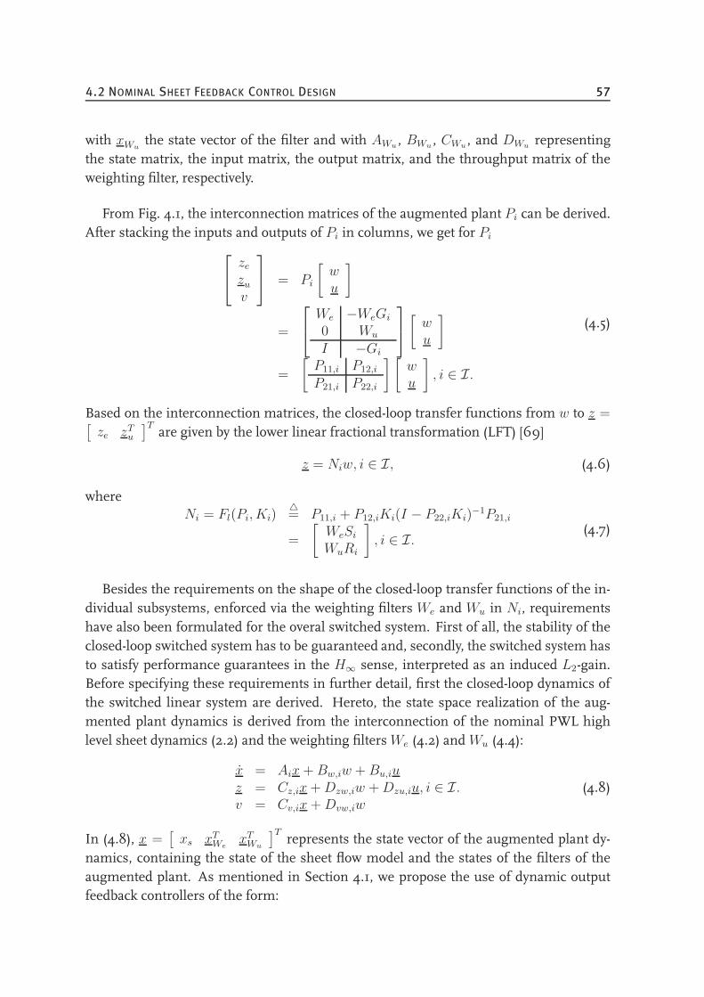
4.2 NOMINAL SHEET FEEDBACK CONTROL DESIGN 57
with xWuthe state vector of the filter and with AWu
, BWu, CWu
, and DWurepresenting
the state matrix, the input matrix, the output matrix, and the throughput matrix of theweighting filter, respectively.
From Fig. 4.1, the interconnection matrices of the augmented plant Pi can be derived.After stacking the inputs and outputs of Pi in columns, we get for Pi
zezuv
= Pi
[wu
]
=
We −WeGi
0 Wu
I −Gi
[wu
]
=
[P11,i P12,i
P21,i P22,i
] [wu
], i ∈ I.
(4.5)
Based on the interconnection matrices, the closed-loop transfer functions from w to z =[ze zTu
]Tare given by the lower linear fractional transformation (LFT) [69]
z = Niw, i ∈ I, (4.6)
whereNi = Fl(Pi, Ki)
= P11,i + P12,iKi(I − P22,iKi)
−1P21,i
=
[WeSiWuRi
], i ∈ I.
(4.7)
Besides the requirements on the shape of the closed-loop transfer functions of the in-dividual subsystems, enforced via the weighting filters We and Wu in Ni, requirementshave also been formulated for the overal switched system. First of all, the stability of theclosed-loop switched system has to be guaranteed and, secondly, the switched system hasto satisfy performance guarantees in the H∞ sense, interpreted as an induced L2-gain.Before specifying these requirements in further detail, first the closed-loop dynamics ofthe switched linear system are derived. Hereto, the state space realization of the aug-mented plant dynamics is derived from the interconnection of the nominal PWL highlevel sheet dynamics (2.2) and the weighting filtersWe (4.2) andWu (4.4):
x = Aix+Bw,iw +Bu,iuz = Cz,ix+Dzw,iw +Dzu,iu, i ∈ I.v = Cv,ix+Dvw,iw
(4.8)
In (4.8), x =[xs xTWe
xTWu
]Trepresents the state vector of the augmented plant dy-
namics, containing the state of the sheet flow model and the states of the filters of theaugmented plant. As mentioned in Section 4.1, we propose the use of dynamic outputfeedback controllers of the form:
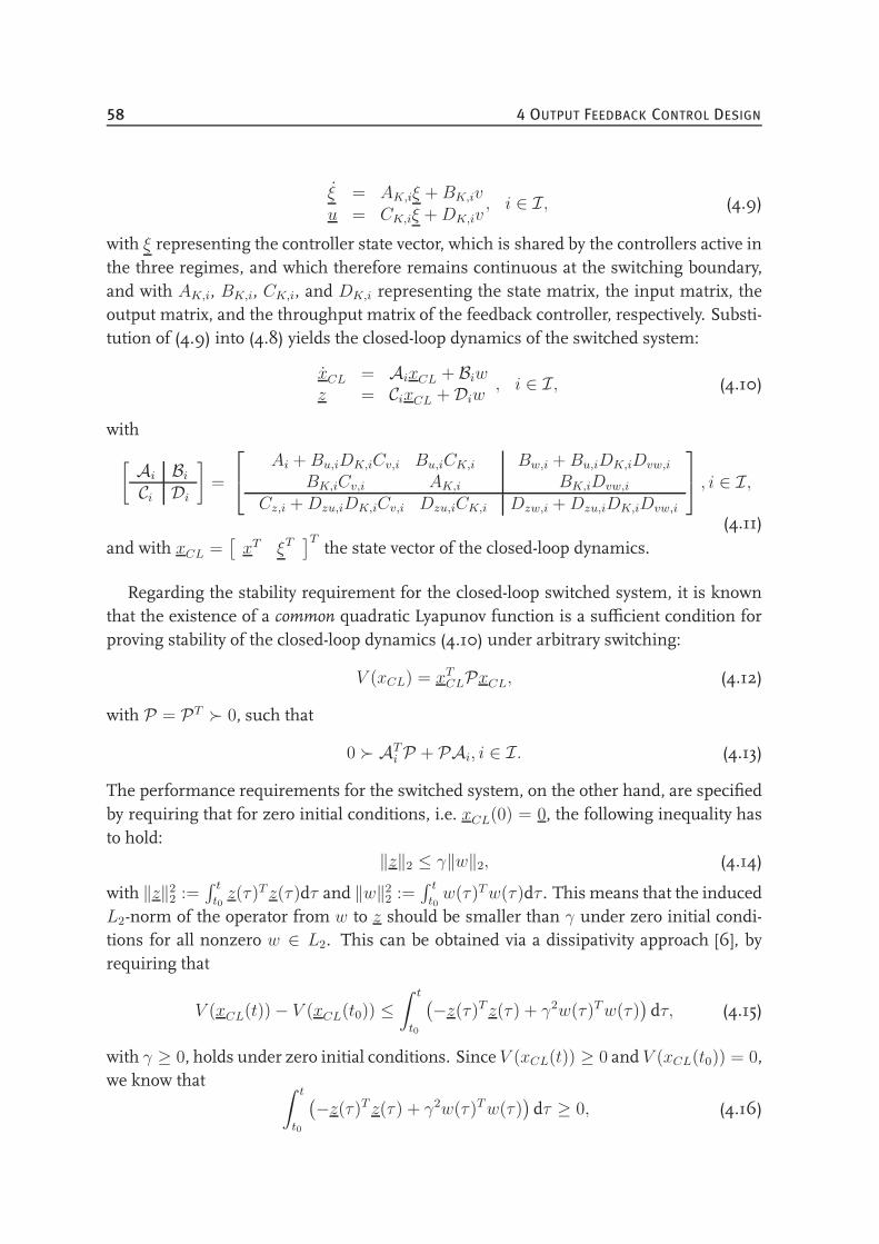
58 4 OUTPUT FEEDBACK CONTROL DESIGN
ξ = AK,iξ +BK,ivu = CK,iξ +DK,iv
, i ∈ I, (4.9)
with ξ representing the controller state vector, which is shared by the controllers active inthe three regimes, and which therefore remains continuous at the switching boundary,and with AK,i, BK,i, CK,i, and DK,i representing the state matrix, the input matrix, theoutput matrix, and the throughput matrix of the feedback controller, respectively. Substi-tution of (4.9) into (4.8) yields the closed-loop dynamics of the switched system:
xCL = AixCL + Biwz = CixCL + Diw
, i ∈ I, (4.10)
with
[Ai BiCi Di
]=
Ai +Bu,iDK,iCv,i Bu,iCK,i
BK,iCv,i AK,i
Bw,i +Bu,iDK,iDvw,i
BK,iDvw,i
Cz,i +Dzu,iDK,iCv,i Dzu,iCK,i Dzw,i +Dzu,iDK,iDvw,i
, i ∈ I,
(4.11)
and with xCL =[xT ξT
]Tthe state vector of the closed-loop dynamics.
Regarding the stability requirement for the closed-loop switched system, it is knownthat the existence of a common quadratic Lyapunov function is a sufficient condition forproving stability of the closed-loop dynamics (4.10) under arbitrary switching:
V (xCL) = xTCLPxCL, (4.12)
with P = PT ≻ 0, such that
0 ≻ ATi P + PAi, i ∈ I. (4.13)
The performance requirements for the switched system, on the other hand, are specifiedby requiring that for zero initial conditions, i.e. xCL(0) = 0, the following inequality hasto hold:
‖z‖2 ≤ γ‖w‖2, (4.14)
with ‖z‖22 :=
∫ t
t0z(τ)T z(τ)dτ and ‖w‖2
2 :=∫ t
t0w(τ)Tw(τ)dτ . This means that the induced
L2-norm of the operator from w to z should be smaller than γ under zero initial condi-tions for all nonzero w ∈ L2. This can be obtained via a dissipativity approach [6], byrequiring that
V (xCL(t)) − V (xCL(t0)) ≤
∫ t
t0
(−z(τ)T z(τ) + γ2w(τ)Tw(τ)
)dτ, (4.15)
with γ ≥ 0, holds under zero initial conditions. Since V (xCL(t)) ≥ 0 and V (xCL(t0)) = 0,we know that ∫ t
t0
(−z(τ)T z(τ) + γ2w(τ)Tw(τ)
)dτ ≥ 0, (4.16)
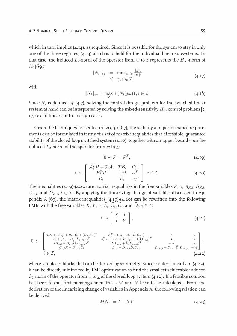
4.2 NOMINAL SHEET FEEDBACK CONTROL DESIGN 59
which in turn implies (4.14), as required. Since it is possible for the system to stay in onlyone of the three regimes, (4.14) also has to hold for the individual linear subsystems. Inthat case, the induced L2-norm of the operator from w to z represents the H∞-norm ofNi [69]:
‖Ni‖∞ = maxw 6=0‖z‖2‖w‖2
≤ γ, i ∈ I,(4.17)
with‖Ni‖∞ = max
ωσ (Ni(jω)) , i ∈ I. (4.18)
Since Ni is defined by (4.7), solving the control design problem for the switched linearsystem at hand can be interpreted by solving themixed-sensitivityH∞ control problem [5,17, 69] in linear control design cases.
Given the techniques presented in [29, 30, 67], the stability and performance require-ments can be formulated in terms of a set of matrix inequalities that, if feasible, guaranteestability of the closed-loop switched system (4.10), together with an upper bound γ on theinduced L2-norm of the operator from w to z:
0 ≺ P = PT , (4.19)
0 ≻
ATi P + PAi PBi CTiBTi P −γI DT
i
Ci Di −γI
, i ∈ I. (4.20)
The inequalities (4.19)-(4.20) are matrix inequalities in the free variables P , γ, AK,i, BK,i,CK,i, and DK,i, i ∈ I. By applying the linearizing change of variables discussed in Ap-pendix A [67], the matrix inequalities (4.19)-(4.20) can be rewritten into the followingLMIs with the free variablesX , Y , γ, Ai, Bi, Ci, and Di, i ∈ I:
0 ≺
[X II Y
], (4.21)
0 ≻
AiX +XAT
i +Bu,iCi + (Bu,iCi)T ATi + (Ai + Bu,iDiCv,i) ⋆ ⋆
Ai + (Ai +Bu,iDiCv,i)T ATi Y + Y Ai + BiCv,i + (BiCv,i)T ⋆ ⋆
(Bw,i +Bu,iDiDvw,i)T (Y Bw,i + BiDvw,i)
T −γI ⋆
Cz,iX +Dzu,iCi Cz,i +Dzu,iDiCv,i Dzw,i +Dzu,iDiDvw,i −γI
,
i ∈ I, (4.22)
where ⋆ replaces blocks that can be derived by symmetry. Since γ enters linearly in (4.22),it can be directly minimized by LMI optimization to find the smallest achievable inducedL2-norm of the operator fromw to z of the closed-loop system (4.10). If a feasible solutionhas been found, first nonsingular matrices M and N have to be calculated. From thederivation of the linearizing change of variables in Appendix A, the following relation canbe derived:
MNT = I −XY. (4.23)
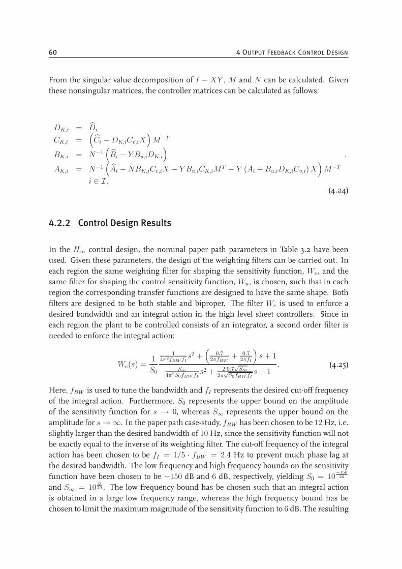
60 4 OUTPUT FEEDBACK CONTROL DESIGN
From the singular value decomposition of I − XY , M and N can be calculated. Giventhese nonsingular matrices, the controller matrices can be calculated as follows:
DK,i = Di
CK,i =(Ci −DK,iCv,iX
)M−T
BK,i = N−1(Bi − Y Bu,iDK,i
)
AK,i = N−1(Ai −NBK,iCv,iX − Y Bu,iCK,iM
T − Y (Ai +Bu,iDK,iCv,i)X)M−T
i ∈ I.
,
(4.24)
4.2.2 Control Design Results
In the H∞ control design, the nominal paper path parameters in Table 3.2 have beenused. Given these parameters, the design of the weighting filters can be carried out. Ineach region the same weighting filter for shaping the sensitivity function, We, and thesame filter for shaping the control sensitivity function, Wu, is chosen, such that in eachregion the corresponding transfer functions are designed to have the same shape. Bothfilters are designed to be both stable and biproper. The filter We is used to enforce adesired bandwidth and an integral action in the high level sheet controllers. Since ineach region the plant to be controlled consists of an integrator, a second order filter isneeded to enforce the integral action:
We(s) =1
S0
14π2fBW fI
s2 +(
0.72πfBW
+ 0.72πfI
)s+ 1
S∞
4π2S0fBW fIs2 + 2·0.7
√S∞
2π√S0fBW fI
s+ 1. (4.25)
Here, fBW is used to tune the bandwidth and fI represents the desired cut-off frequencyof the integral action. Furthermore, S0 represents the upper bound on the amplitudeof the sensitivity function for s → 0, whereas S∞ represents the upper bound on theamplitude for s→ ∞. In the paper path case-study, fBW has been chosen to be 12 Hz, i.e.slightly larger than the desired bandwidth of 10 Hz, since the sensitivity function will notbe exactly equal to the inverse of its weighting filter. The cut-off frequency of the integralaction has been chosen to be fI = 1/5 · fBW = 2.4 Hz to prevent much phase lag atthe desired bandwidth. The low frequency and high frequency bounds on the sensitivityfunction have been chosen to be −150 dB and 6 dB, respectively, yielding S0 = 10
−150
20
and S∞ = 106
20 . The low frequency bound has be chosen such that an integral actionis obtained in a large low frequency range, whereas the high frequency bound has bechosen to limit the maximummagnitude of the sensitivity function to 6 dB. The resulting
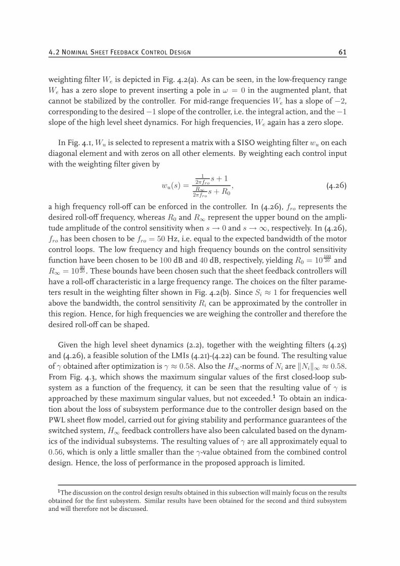
4.2 NOMINAL SHEET FEEDBACK CONTROL DESIGN 61
weighting filterWe is depicted in Fig. 4.2(a). As can be seen, in the low-frequency rangeWe has a zero slope to prevent inserting a pole in ω = 0 in the augmented plant, thatcannot be stabilized by the controller. For mid-range frequencies We has a slope of −2,corresponding to the desired−1 slope of the controller, i.e. the integral action, and the−1
slope of the high level sheet dynamics. For high frequencies,We again has a zero slope.
In Fig. 4.1,Wu is selected to represent a matrix with a SISO weighting filterwu on eachdiagonal element and with zeros on all other elements. By weighting each control inputwith the weighting filter given by
wu(s) =
12πfro
s+ 1R∞
2πfros+R0
, (4.26)
a high frequency roll-off can be enforced in the controller. In (4.26), fro represents thedesired roll-off frequency, whereas R0 and R∞ represent the upper bound on the ampli-tude amplitude of the control sensitivity when s→ 0 and s→ ∞, respectively. In (4.26),fro has been chosen to be fro = 50 Hz, i.e. equal to the expected bandwidth of the motorcontrol loops. The low frequency and high frequency bounds on the control sensitivityfunction have been chosen to be 100 dB and 40 dB, respectively, yielding R0 = 10
100
20 andR∞ = 10
40
20 . These bounds have been chosen such that the sheet feedback controllers willhave a roll-off characteristic in a large frequency range. The choices on the filter parame-ters result in the weighting filter shown in Fig. 4.2(b). Since Si ≈ 1 for frequencies wellabove the bandwidth, the control sensitivity Ri can be approximated by the controller inthis region. Hence, for high frequencies we are weighing the controller and therefore thedesired roll-off can be shaped.
Given the high level sheet dynamics (2.2), together with the weighting filters (4.25)and (4.26), a feasible solution of the LMIs (4.21)-(4.22) can be found. The resulting valueof γ obtained after optimization is γ ≈ 0.58. Also theH∞-norms of Ni are ‖Ni‖∞ ≈ 0.58.From Fig. 4.3, which shows the maximum singular values of the first closed-loop sub-system as a function of the frequency, it can be seen that the resulting value of γ isapproached by these maximum singular values, but not exceeded.1 To obtain an indica-tion about the loss of subsystem performance due to the controller design based on thePWL sheet flow model, carried out for giving stability and performance guarantees of theswitched system,H∞ feedback controllers have also been calculated based on the dynam-ics of the individual subsystems. The resulting values of γ are all approximately equal to0.56, which is only a little smaller than the γ-value obtained from the combined controldesign. Hence, the loss of performance in the proposed approach is limited.
1The discussion on the control design results obtained in this subsection will mainly focus on the resultsobtained for the first subsystem. Similar results have been obtained for the second and third subsystemand will therefore not be discussed.
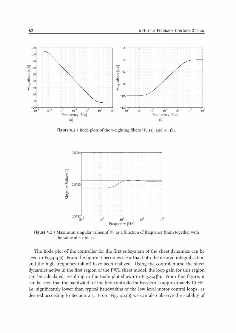
62 4 OUTPUT FEEDBACK CONTROL DESIGN
10−4
10−3
10−2
10−1
100
101
102
−20
0
20
40
60
80
100
120
140
160
Magnitude
[dB]
Frequency [Hz](a)
100
101
102
103
104
105
106
−120
−100
−80
−60
−40
−20
Magnitude
[dB]
Frequency [Hz](b)
Figure 4.2 / Bode plots of the weighting filters We (a), and wu (b).
10−1
100
101
102
103
0.5792
0.5793
0.5794
Singu
larValues
[-]
Frequency [Hz]
Figure 4.3 /Maximum singular values of N1 as a function of frequency (thin) together withthe value of γ (thick).
The Bode plot of the controller for the first subsystem of the sheet dynamics can beseen in Fig.4.4(a). From the figure it becomes clear that both the desired integral actionand the high frequency roll-off have been realized. Using the controller and the sheetdynamics active in the first region of the PWL sheet model, the loop gain for this regioncan be calculated, resulting in the Bode plot shown in Fig.4.4(b). From this figure, itcan be seen that the bandwidth of the first controlled subsystem is approximately 10 Hz,i.e. significantly lower than typical bandwidths of the low level motor control loops, asdesired according to Section 2.3. From Fig. 4.4(b) we can also observe the stability of
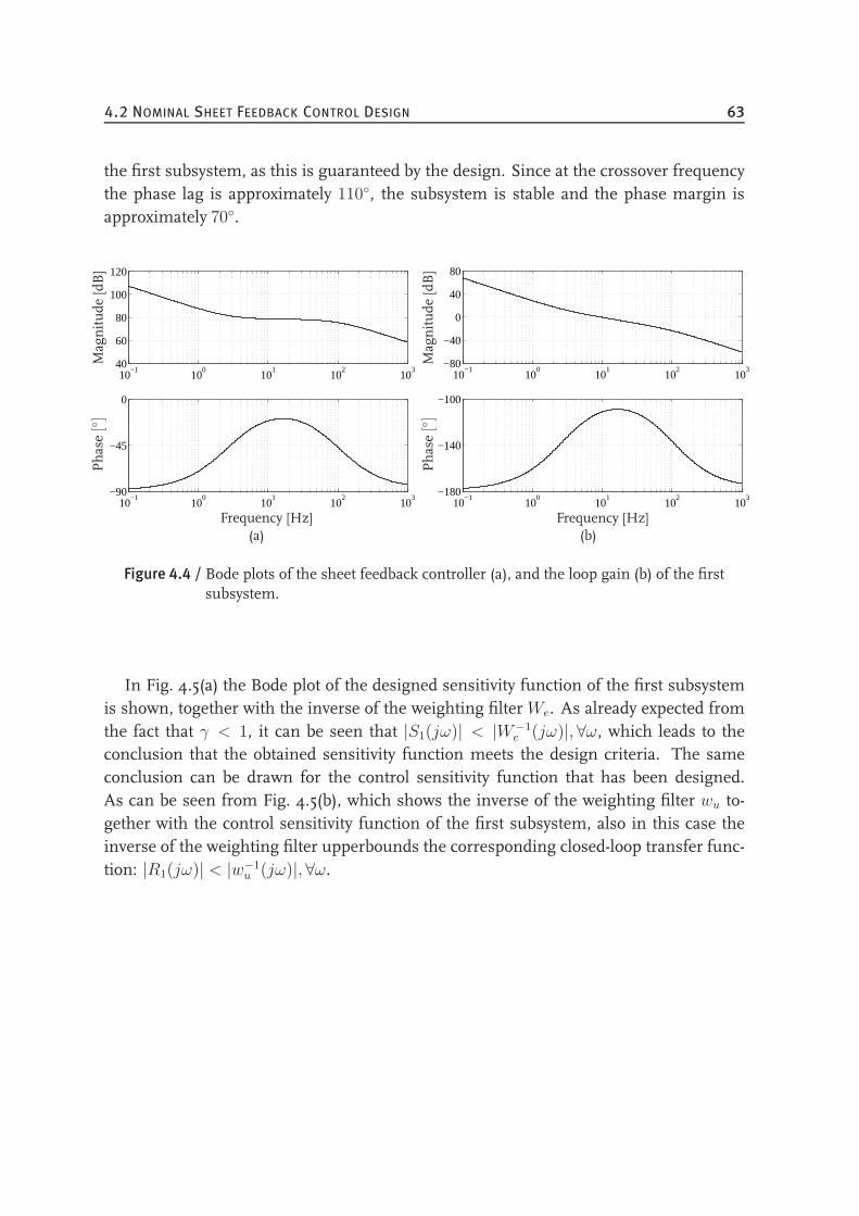
4.2 NOMINAL SHEET FEEDBACK CONTROL DESIGN 63
the first subsystem, as this is guaranteed by the design. Since at the crossover frequencythe phase lag is approximately 110, the subsystem is stable and the phase margin isapproximately 70.
10−1
100
101
102
103
40
60
80
100
120
10−1
100
101
102
103
−90
−45
0
Magnitude
[dB]
Phase
[]
Frequency [Hz](a)
10−1
100
101
102
103
−80
−40
0
40
80
10−1
100
101
102
103
−180
−140
−100
Magnitude
[dB]
Phase
[]
Frequency [Hz](b)
Figure 4.4 / Bode plots of the sheet feedback controller (a), and the loop gain (b) of the firstsubsystem.
In Fig. 4.5(a) the Bode plot of the designed sensitivity function of the first subsystemis shown, together with the inverse of the weighting filterWe. As already expected fromthe fact that γ < 1, it can be seen that |S1(jω)| < |W−1
e (jω)|, ∀ω, which leads to theconclusion that the obtained sensitivity function meets the design criteria. The sameconclusion can be drawn for the control sensitivity function that has been designed.As can be seen from Fig. 4.5(b), which shows the inverse of the weighting filter wu to-gether with the control sensitivity function of the first subsystem, also in this case theinverse of the weighting filter upperbounds the corresponding closed-loop transfer func-tion: |R1(jω)| < |w−1
u (jω)|, ∀ω.
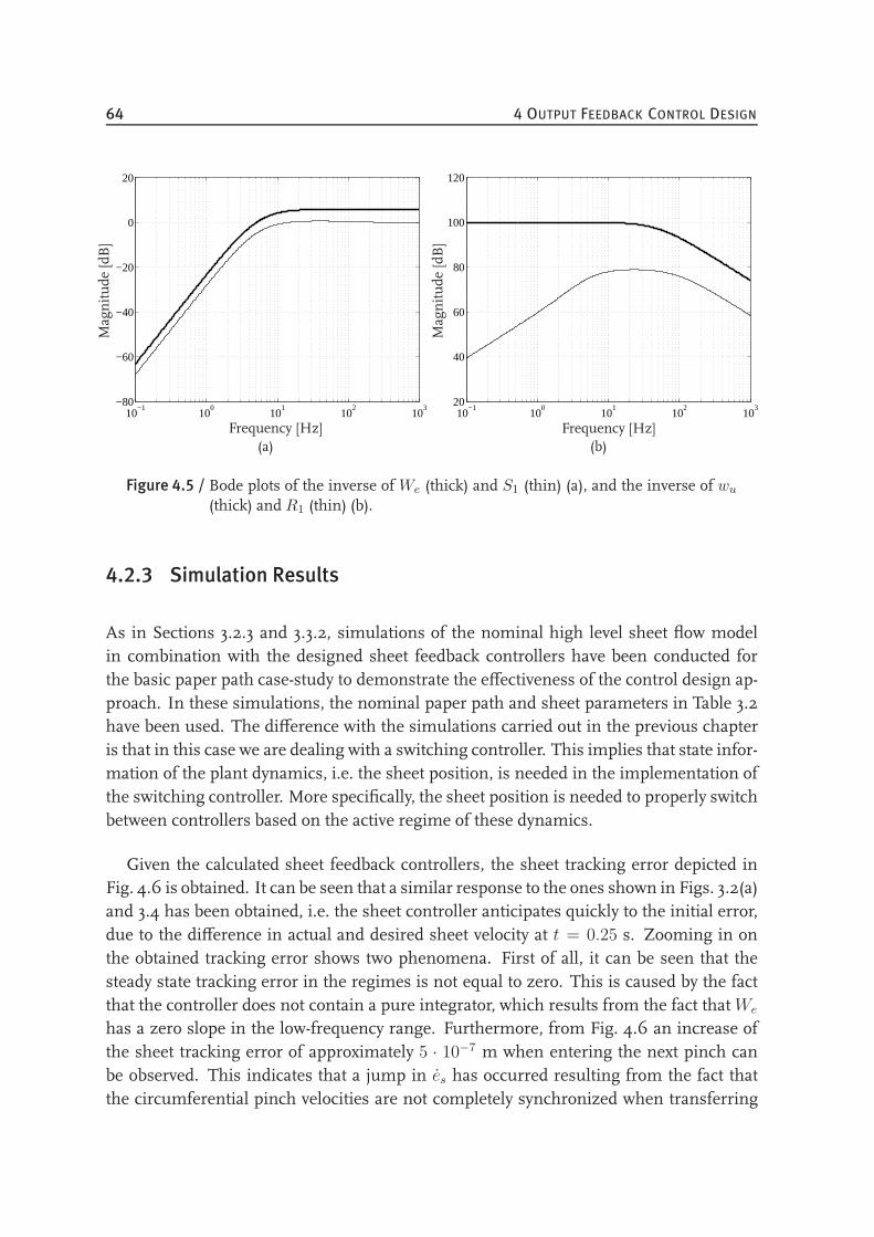
64 4 OUTPUT FEEDBACK CONTROL DESIGN
10−1
100
101
102
103
−80
−60
−40
−20
0
20
Magnitude
[dB]
Frequency [Hz](a)
10−1
100
101
102
103
20
40
60
80
100
120
Magnitude
[dB]
Frequency [Hz](b)
Figure 4.5 / Bode plots of the inverse of We (thick) and S1 (thin) (a), and the inverse of wu(thick) and R1 (thin) (b).
4.2.3 Simulation Results
As in Sections 3.2.3 and 3.3.2, simulations of the nominal high level sheet flow modelin combination with the designed sheet feedback controllers have been conducted forthe basic paper path case-study to demonstrate the effectiveness of the control design ap-proach. In these simulations, the nominal paper path and sheet parameters in Table 3.2have been used. The difference with the simulations carried out in the previous chapteris that in this case we are dealing with a switching controller. This implies that state infor-mation of the plant dynamics, i.e. the sheet position, is needed in the implementation ofthe switching controller. More specifically, the sheet position is needed to properly switchbetween controllers based on the active regime of these dynamics.
Given the calculated sheet feedback controllers, the sheet tracking error depicted inFig. 4.6 is obtained. It can be seen that a similar response to the ones shown in Figs. 3.2(a)and 3.4 has been obtained, i.e. the sheet controller anticipates quickly to the initial error,due to the difference in actual and desired sheet velocity at t = 0.25 s. Zooming in onthe obtained tracking error shows two phenomena. First of all, it can be seen that thesteady state tracking error in the regimes is not equal to zero. This is caused by the factthat the controller does not contain a pure integrator, which results from the fact thatWe
has a zero slope in the low-frequency range. Furthermore, from Fig. 4.6 an increase ofthe sheet tracking error of approximately 5 · 10−7 m when entering the next pinch canbe observed. This indicates that a jump in es has occurred resulting from the fact thatthe circumferential pinch velocities are not completely synchronized when transferring
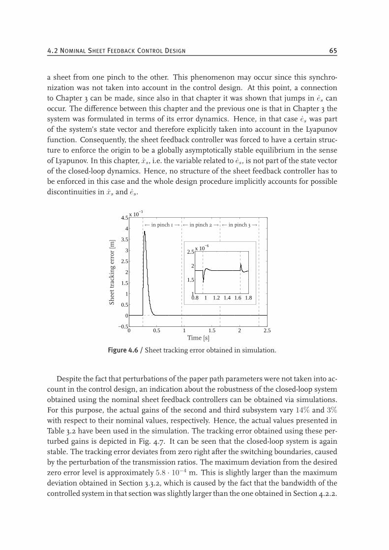
4.2 NOMINAL SHEET FEEDBACK CONTROL DESIGN 65
a sheet from one pinch to the other. This phenomenon may occur since this synchro-nization was not taken into account in the control design. At this point, a connectionto Chapter 3 can be made, since also in that chapter it was shown that jumps in es canoccur. The difference between this chapter and the previous one is that in Chapter 3 thesystem was formulated in terms of its error dynamics. Hence, in that case es was partof the system’s state vector and therefore explicitly taken into account in the Lyapunovfunction. Consequently, the sheet feedback controller was forced to have a certain struc-ture to enforce the origin to be a globally asymptotically stable equilibrium in the senseof Lyapunov. In this chapter, xs, i.e. the variable related to es, is not part of the state vectorof the closed-loop dynamics. Hence, no structure of the sheet feedback controller has tobe enforced in this case and the whole design procedure implicitly accounts for possiblediscontinuities in xs and es.
0 0.5 1 1.5 2 2.5−0.5
0
0.5
1
1.5
2
2.5
3
3.5
4
4.5x 10
−3
0.8 1 1.2 1.4 1.6 1.81
1.5
2
2.5x 10
−6
Time [s]
Sheettrackingerror[m
]
← in pinch 1→ ← in pinch 2→ ← in pinch 3→
Figure 4.6 / Sheet tracking error obtained in simulation.
Despite the fact that perturbations of the paper path parameters were not taken into ac-count in the control design, an indication about the robustness of the closed-loop systemobtained using the nominal sheet feedback controllers can be obtained via simulations.For this purpose, the actual gains of the second and third subsystem vary 14% and 3%
with respect to their nominal values, respectively. Hence, the actual values presented inTable 3.2 have been used in the simulation. The tracking error obtained using these per-turbed gains is depicted in Fig. 4.7. It can be seen that the closed-loop system is againstable. The tracking error deviates from zero right after the switching boundaries, causedby the perturbation of the transmission ratios. The maximum deviation from the desiredzero error level is approximately 5.8 · 10−4 m. This is slightly larger than the maximumdeviation obtained in Section 3.3.2, which is caused by the fact that the bandwidth of thecontrolled system in that section was slightly larger than the one obtained in Section 4.2.2.
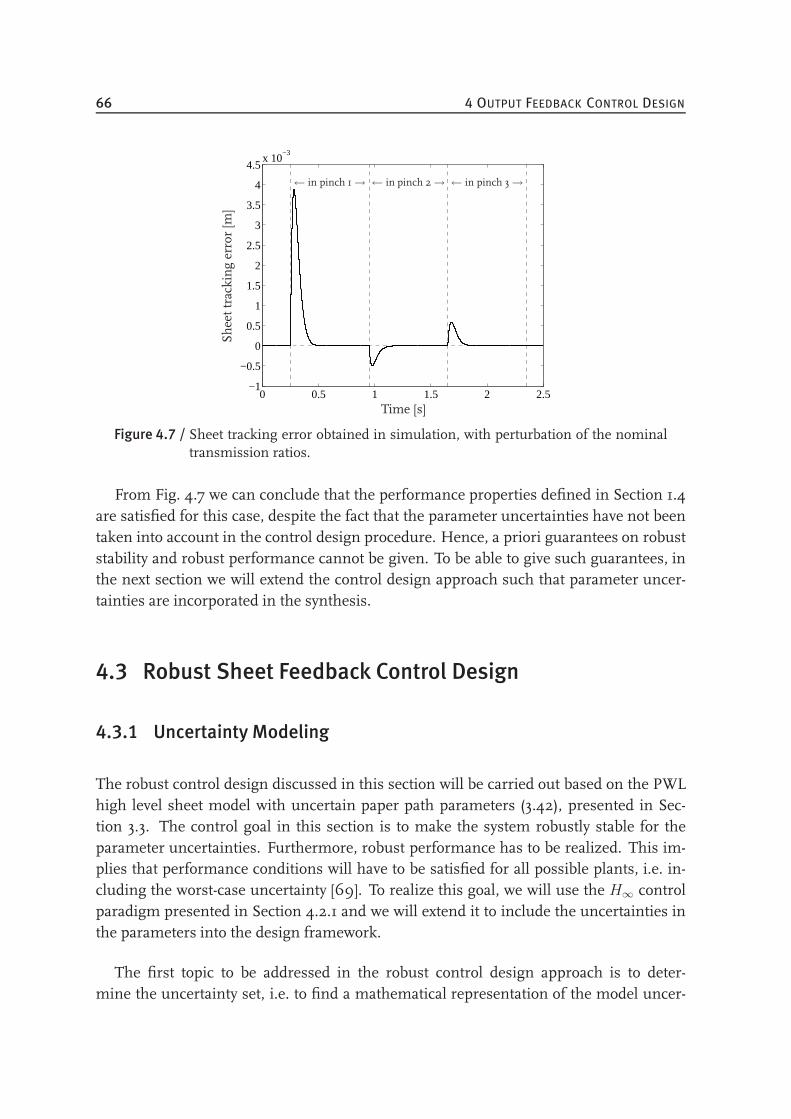
66 4 OUTPUT FEEDBACK CONTROL DESIGN
0 0.5 1 1.5 2 2.5−1
−0.5
0
0.5
1
1.5
2
2.5
3
3.5
4
4.5x 10
−3
Time [s]
Sheettrackingerror[m
]
← in pinch 1→ ← in pinch 2→ ← in pinch 3→
Figure 4.7 / Sheet tracking error obtained in simulation, with perturbation of the nominaltransmission ratios.
From Fig. 4.7 we can conclude that the performance properties defined in Section 1.4are satisfied for this case, despite the fact that the parameter uncertainties have not beentaken into account in the control design procedure. Hence, a priori guarantees on robuststability and robust performance cannot be given. To be able to give such guarantees, inthe next section we will extend the control design approach such that parameter uncer-tainties are incorporated in the synthesis.
4.3 Robust Sheet Feedback Control Design
4.3.1 Uncertainty Modeling
The robust control design discussed in this section will be carried out based on the PWLhigh level sheet model with uncertain paper path parameters (3.42), presented in Sec-tion 3.3. The control goal in this section is to make the system robustly stable for theparameter uncertainties. Furthermore, robust performance has to be realized. This im-plies that performance conditions will have to be satisfied for all possible plants, i.e. in-cluding the worst-case uncertainty [69]. To realize this goal, we will use the H∞ controlparadigm presented in Section 4.2.1 and we will extend it to include the uncertainties inthe parameters into the design framework.
The first topic to be addressed in the robust control design approach is to deter-mine the uncertainty set, i.e. to find a mathematical representation of the model uncer-
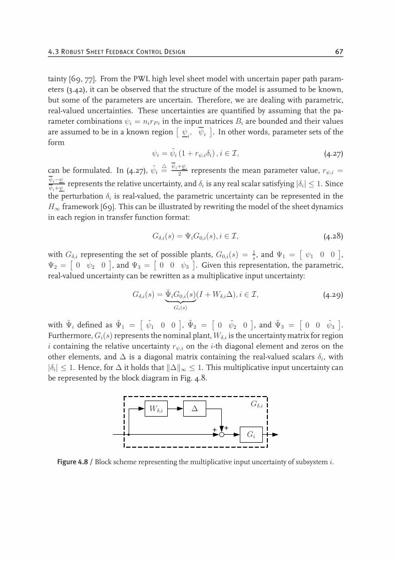
4.3 ROBUST SHEET FEEDBACK CONTROL DESIGN 67
tainty [69, 77]. From the PWL high level sheet model with uncertain paper path param-eters (3.42), it can be observed that the structure of the model is assumed to be known,but some of the parameters are uncertain. Therefore, we are dealing with parametric,real-valued uncertainties. These uncertainties are quantified by assuming that the pa-rameter combinations ψi = nirPi in the input matrices Bi are bounded and their valuesare assumed to be in a known region
[ψi, ψi
]. In other words, parameter sets of the
formψi = ψi (1 + rψ,iδi) , i ∈ I, (4.27)
can be formulated. In (4.27), ψi=
ψi+ψi
2represents the mean parameter value, rψ,i =
ψi−ψi
ψi+ψi
represents the relative uncertainty, and δi is any real scalar satisfying |δi| ≤ 1. Since
the perturbation δi is real-valued, the parametric uncertainty can be represented in theH∞ framework [69]. This can be illustrated by rewriting the model of the sheet dynamicsin each region in transfer function format:
Gδ,i(s) = ΨiG0,i(s), i ∈ I, (4.28)
with Gδ,i representing the set of possible plants, G0,i(s) = 1s, and Ψ1 =
[ψ1 0 0
],
Ψ2 =[
0 ψ2 0], and Ψ3 =
[0 0 ψ3
]. Given this representation, the parametric,
real-valued uncertainty can be rewritten as a multiplicative input uncertainty:
Gδ,i(s) = ΨiG0,i(s)︸ ︷︷ ︸Gi(s)
(I +Wδ,i∆), i ∈ I, (4.29)
with Ψi defined as Ψ1 =[ψ1 0 0
], Ψ2 =
[0 ψ2 0
], and Ψ3 =
[0 0 ψ3
].
Furthermore,Gi(s) represents the nominal plant,Wδ,i is the uncertaintymatrix for regioni containing the relative uncertainty rψ,i on the i-th diagonal element and zeros on theother elements, and ∆ is a diagonal matrix containing the real-valued scalars δi, with|δi| ≤ 1. Hence, for ∆ it holds that ‖∆‖∞ ≤ 1. This multiplicative input uncertainty canbe represented by the block diagram in Fig. 4.8.
+ +
Wδ,i ∆Gδ,i
Gi
Figure 4.8 / Block scheme representing the multiplicative input uncertainty of subsystem i.
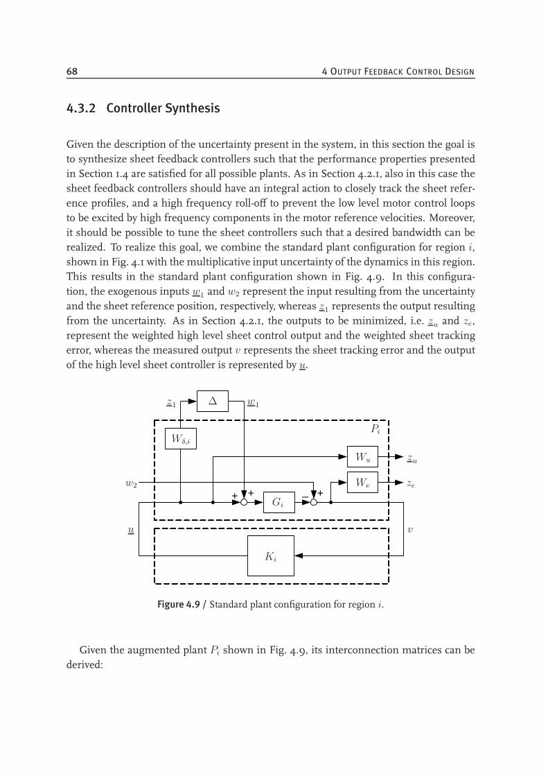
68 4 OUTPUT FEEDBACK CONTROL DESIGN
4.3.2 Controller Synthesis
Given the description of the uncertainty present in the system, in this section the goal isto synthesize sheet feedback controllers such that the performance properties presentedin Section 1.4 are satisfied for all possible plants. As in Section 4.2.1, also in this case thesheet feedback controllers should have an integral action to closely track the sheet refer-ence profiles, and a high frequency roll-off to prevent the low level motor control loopsto be excited by high frequency components in the motor reference velocities. Moreover,it should be possible to tune the sheet controllers such that a desired bandwidth can berealized. To realize this goal, we combine the standard plant configuration for region i,shown in Fig. 4.1 with the multiplicative input uncertainty of the dynamics in this region.This results in the standard plant configuration shown in Fig. 4.9. In this configura-tion, the exogenous inputs w1 and w2 represent the input resulting from the uncertaintyand the sheet reference position, respectively, whereas z1 represents the output resultingfrom the uncertainty. As in Section 4.2.1, the outputs to be minimized, i.e. zu and ze,represent the weighted high level sheet control output and the weighted sheet trackingerror, whereas the measured output v represents the sheet tracking error and the outputof the high level sheet controller is represented by u.
_ ++ +
Wu
We
Gi
Pi
Ki
w2
u v
ze
zu
Wδ,i
∆ w1z1
Figure 4.9 / Standard plant configuration for region i.
Given the augmented plant Pi shown in Fig. 4.9, its interconnection matrices can bederived:
4.3 ROBUST SHEET FEEDBACK CONTROL DESIGN 69
z1
zezuv
= Pi
w1
w2
u
=
0 0 Wδ,i
−WeGi We −WeGi
0 0 Wu
−Gi I −Gi
w1
w2
u
, i ∈ I.
(4.30)
Based on the interconnection matrices, the closed-loop transfer functions from w =[wT1 w2
]Tto z =
[zT1 ze zTu
]Tare again given by the lower LFT
z = Niw, i ∈ I, (4.31)
with
Ni =
−Wδ,iTi Wδ,iRi
−WeSp,i WeSi−WuTi WuRi
, i ∈ I. (4.32)
In (4.32)Ti = (I +KiGi)
−1KiGi, i ∈ I, (4.33)
represents the (input) complementary sensitivity function of subsystem i, whereas
Sp,i = (I +GiKi)−1Gi, i ∈ I, (4.34)
represents the (output) process sensitivity function. By inspection of (4.32) it can beseen thatWe will affect both the sensitivity function and the process sensitivity function.Since this filter is designed to weigh the sensitivity function to create an integral action inthe controller at low frequencies, applying this weight to the process sensitivity functionwill result in a penalty at low frequencies that is too demanding, resulting in a doubleintegral action in the controller. To avoid this, a different standard plant configurationwill be used, which is shown in Fig. 4.10. In this configuration, the exogenous input w2
is chosen as a disturbance acting on the high level sheet control output u, instead of thesheet reference position. This choice does not change our control problem, as we usethis control design approach to shape certain closed-loop transfer functions. Since theoutputs to be minimized, i.e. zu and zy represent in this case the weighted high levelsheet control output and the weighted high level plant output, respectively, weighing ofthe complementary sensitivity function and the process sensitivity function is possible.The weighting filterWu penalizes the control input u and can therefore be used to enforcea high frequency roll-off in the controller. Furthermore, in combination with the filterWy,it can be used to realize the desired bandwidth of the controlled system. Furthermore, thefilter Wy is used for penalizing the plant output y and can therefore be used to enforcethe integral action action in the controller. Both filters can be represented in analogywith (4.4) and (4.2), respectively.
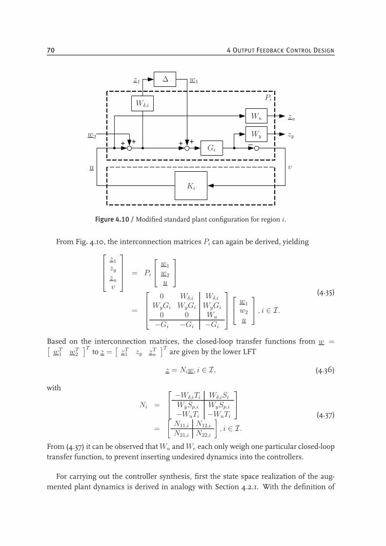
70 4 OUTPUT FEEDBACK CONTROL DESIGN
+ + ++ _
Wu
Wy
Gi
Pi
Ki
w2
u v
zy
zu
Wδ,i
∆ w1z1
Figure 4.10 / Modified standard plant configuration for region i.
From Fig. 4.10, the interconnection matrices Pi can again be derived, yielding
z1
zyzuv
= Pi
w1
w2
u
=
0 Wδ,i Wδ,i
WyGi WyGi WyGi
0 0 Wu
−Gi −Gi −Gi
w1
w2
u
, i ∈ I.
(4.35)
Based on the interconnection matrices, the closed-loop transfer functions from w =[wT1 wT2
]Tto z =
[zT1 zy zTu
]Tare given by the lower LFT
z = Niw, i ∈ I, (4.36)
with
Ni =
−Wδ,iTi Wδ,iSiWySp,i WySp,i−WuTi −WuTi
=
[N11,i N12,i
N21,i N22,i
], i ∈ I.
(4.37)
From (4.37) it can be observed thatWu andWe each only weigh one particular closed-looptransfer function, to prevent inserting undesired dynamics into the controllers.
For carrying out the controller synthesis, first the state space realization of the aug-mented plant dynamics is derived in analogy with Section 4.2.1. With the definition of
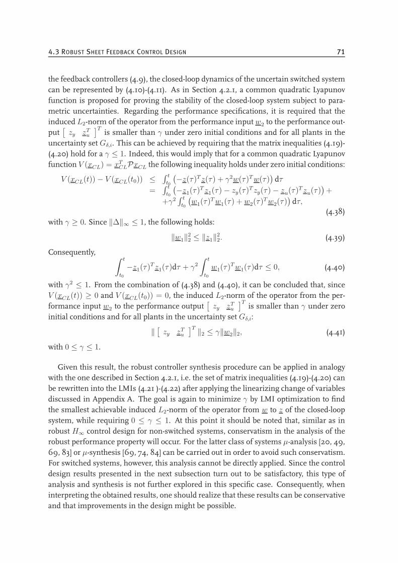
4.3 ROBUST SHEET FEEDBACK CONTROL DESIGN 71
the feedback controllers (4.9), the closed-loop dynamics of the uncertain switched systemcan be represented by (4.10)-(4.11). As in Section 4.2.1, a common quadratic Lyapunovfunction is proposed for proving the stability of the closed-loop system subject to para-metric uncertainties. Regarding the performance specifications, it is required that theinduced L2-norm of the operator from the performance input w2 to the performance out-put
[zy zTu
]Tis smaller than γ under zero initial conditions and for all plants in the
uncertainty set Gδ,i. This can be achieved by requiring that the matrix inequalities (4.19)-(4.20) hold for a γ ≤ 1. Indeed, this would imply that for a common quadratic Lyapunovfunction V (xCL) = xTCLPxCL the following inequality holds under zero initial conditions:
V (xCL(t)) − V (xCL(t0)) ≤∫ t
t0
(−z(τ)T z(τ) + γ2w(τ)Tw(τ)
)dτ
=∫ t
t0
(−z1(τ)
T z1(τ) − zy(τ)T zy(τ) − zu(τ)
T zu(τ))+
+γ2∫ t
t0
(w1(τ)
Tw1(τ) + w2(τ)Tw2(τ)
)dτ,
(4.38)with γ ≥ 0. Since ‖∆‖∞ ≤ 1, the following holds:
‖w1‖22 ≤ ‖z1‖
22. (4.39)
Consequently, ∫ t
t0
−z1(τ)T z1(τ)dτ + γ2
∫ t
t0
w1(τ)Tw1(τ)dτ ≤ 0, (4.40)
with γ2 ≤ 1. From the combination of (4.38) and (4.40), it can be concluded that, sinceV (xCL(t)) ≥ 0 and V (xCL(t0)) = 0, the induced L2-norm of the operator from the per-formance input w2 to the performance output
[zy zTu
]Tis smaller than γ under zero
initial conditions and for all plants in the uncertainty set Gδ,i:
‖[zy zTu
]T‖2 ≤ γ‖w2‖2, (4.41)
with 0 ≤ γ ≤ 1.
Given this result, the robust controller synthesis procedure can be applied in analogywith the one described in Section 4.2.1, i.e. the set of matrix inequalities (4.19)-(4.20) canbe rewritten into the LMIs (4.21 )-(4.22) after applying the linearizing change of variablesdiscussed in Appendix A. The goal is again to minimize γ by LMI optimization to findthe smallest achievable induced L2-norm of the operator from w to z of the closed-loopsystem, while requiring 0 ≤ γ ≤ 1. At this point it should be noted that, similar as inrobust H∞ control design for non-switched systems, conservatism in the analysis of therobust performance property will occur. For the latter class of systems µ-analysis [20, 49,69, 83] or µ-synthesis [69, 74, 84] can be carried out in order to avoid such conservatism.For switched systems, however, this analysis cannot be directly applied. Since the controldesign results presented in the next subsection turn out to be satisfactory, this type ofanalysis and synthesis is not further explored in this specific case. Consequently, wheninterpreting the obtained results, one should realize that these results can be conservativeand that improvements in the design might be possible.
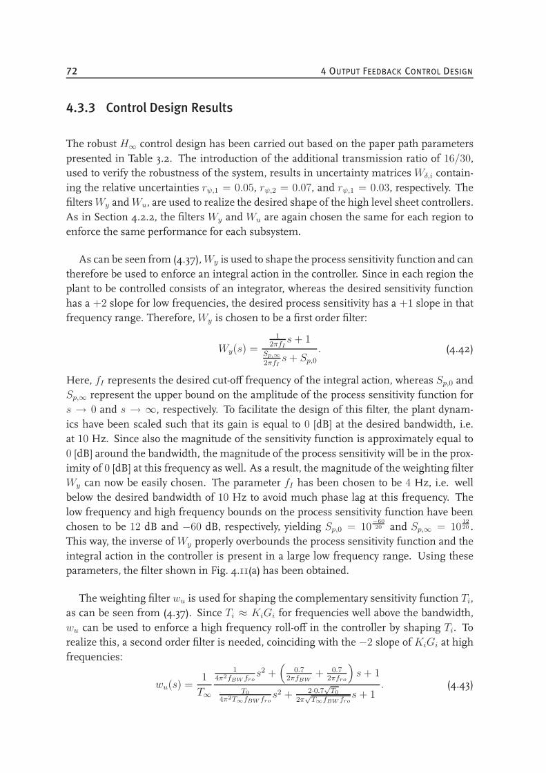
72 4 OUTPUT FEEDBACK CONTROL DESIGN
4.3.3 Control Design Results
The robust H∞ control design has been carried out based on the paper path parameterspresented in Table 3.2. The introduction of the additional transmission ratio of 16/30,used to verify the robustness of the system, results in uncertainty matricesWδ,i contain-ing the relative uncertainties rψ,1 = 0.05, rψ,2 = 0.07, and rψ,1 = 0.03, respectively. ThefiltersWy andWu, are used to realize the desired shape of the high level sheet controllers.As in Section 4.2.2, the filters Wy and Wu are again chosen the same for each region toenforce the same performance for each subsystem.
As can be seen from (4.37),Wy is used to shape the process sensitivity function and cantherefore be used to enforce an integral action in the controller. Since in each region theplant to be controlled consists of an integrator, whereas the desired sensitivity functionhas a +2 slope for low frequencies, the desired process sensitivity has a +1 slope in thatfrequency range. Therefore,Wy is chosen to be a first order filter:
Wy(s) =
12πfI
s+ 1Sp,∞
2πfIs+ Sp,0
. (4.42)
Here, fI represents the desired cut-off frequency of the integral action, whereas Sp,0 andSp,∞ represent the upper bound on the amplitude of the process sensitivity function fors → 0 and s → ∞, respectively. To facilitate the design of this filter, the plant dynam-ics have been scaled such that its gain is equal to 0 [dB] at the desired bandwidth, i.e.at 10 Hz. Since also the magnitude of the sensitivity function is approximately equal to0 [dB] around the bandwidth, the magnitude of the process sensitivity will be in the prox-imity of 0 [dB] at this frequency as well. As a result, the magnitude of the weighting filterWy can now be easily chosen. The parameter fI has been chosen to be 4 Hz, i.e. wellbelow the desired bandwidth of 10 Hz to avoid much phase lag at this frequency. Thelow frequency and high frequency bounds on the process sensitivity function have beenchosen to be 12 dB and −60 dB, respectively, yielding Sp,0 = 10
−60
20 and Sp,∞ = 1012
20 .This way, the inverse ofWy properly overbounds the process sensitivity function and theintegral action in the controller is present in a large low frequency range. Using theseparameters, the filter shown in Fig. 4.11(a) has been obtained.
The weighting filter wu is used for shaping the complementary sensitivity function Ti,as can be seen from (4.37). Since Ti ≈ KiGi for frequencies well above the bandwidth,wu can be used to enforce a high frequency roll-off in the controller by shaping Ti. Torealize this, a second order filter is needed, coinciding with the −2 slope of KiGi at highfrequencies:
wu(s) =1
T∞
14π2fBW fro
s2 +(
0.72πfBW
+ 0.72πfro
)s+ 1
T0
4π2T∞fBW fros2 + 2·0.7
√T0
2π√T∞fBW fro
s+ 1. (4.43)
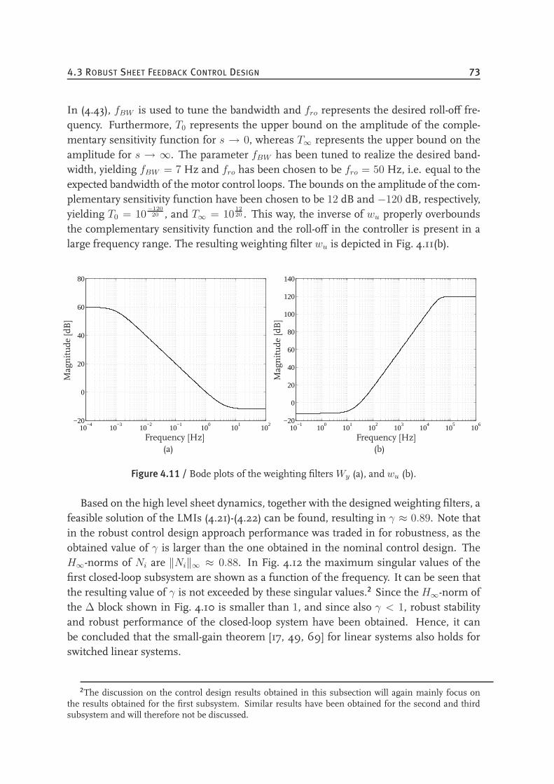
4.3 ROBUST SHEET FEEDBACK CONTROL DESIGN 73
In (4.43), fBW is used to tune the bandwidth and fro represents the desired roll-off fre-quency. Furthermore, T0 represents the upper bound on the amplitude of the comple-mentary sensitivity function for s → 0, whereas T∞ represents the upper bound on theamplitude for s → ∞. The parameter fBW has been tuned to realize the desired band-width, yielding fBW = 7 Hz and fro has been chosen to be fro = 50 Hz, i.e. equal to theexpected bandwidth of the motor control loops. The bounds on the amplitude of the com-plementary sensitivity function have been chosen to be 12 dB and −120 dB, respectively,yielding T0 = 10
−120
20 , and T∞ = 1012
20 . This way, the inverse of wu properly overboundsthe complementary sensitivity function and the roll-off in the controller is present in alarge frequency range. The resulting weighting filter wu is depicted in Fig. 4.11(b).
10−4
10−3
10−2
10−1
100
101
102
−20
0
20
40
60
80
Magnitude
[dB]
Frequency [Hz](a)
10−1
100
101
102
103
104
105
106
−20
0
20
40
60
80
100
120
140Magnitude
[dB]
Frequency [Hz](b)
Figure 4.11 / Bode plots of the weighting filters Wy (a), and wu (b).
Based on the high level sheet dynamics, together with the designed weighting filters, afeasible solution of the LMIs (4.21)-(4.22) can be found, resulting in γ ≈ 0.89. Note thatin the robust control design approach performance was traded in for robustness, as theobtained value of γ is larger than the one obtained in the nominal control design. TheH∞-norms of Ni are ‖Ni‖∞ ≈ 0.88. In Fig. 4.12 the maximum singular values of thefirst closed-loop subsystem are shown as a function of the frequency. It can be seen thatthe resulting value of γ is not exceeded by these singular values.2 Since the H∞-norm ofthe ∆ block shown in Fig. 4.10 is smaller than 1, and since also γ < 1, robust stabilityand robust performance of the closed-loop system have been obtained. Hence, it canbe concluded that the small-gain theorem [17, 49, 69] for linear systems also holds forswitched linear systems.
2The discussion on the control design results obtained in this subsection will again mainly focus onthe results obtained for the first subsystem. Similar results have been obtained for the second and thirdsubsystem and will therefore not be discussed.
74 4 OUTPUT FEEDBACK CONTROL DESIGN
10−1
100
101
102
103
0.82
0.84
0.86
0.88
0.9
Singu
larValues
[-]
Frequency [Hz]
Figure 4.12 / Maximum singular values of N1 as a function of frequency (thin) togetherwith the value of γ (thick).
Also for the robust control design case, controllers have been designed based on thedynamics in the individual subsystems to obtain an indication about the loss of subsystemperformance due to the fact the controller design is based on the PWL sheet flow model.The resulting values of γ are all approximately equal to 0.59, which is smaller than the γ-value obtained from the combined control design. Hence, in case of robust control designbased on the switched dynamics, some subsystem performance is lost in comparison withthe individual control design.
In Fig. 4.13(a), the Bode plot of the controller for the first subsystem of the sheet dy-namics is shown. From the figure it becomes clear that both the desired integral actionand the high frequency roll-off have been realized. Comparing Fig. 4.13(a) with Fig. 4.4(a),a large difference in gain can be noticed. This is due to the scaling of the plant in the de-sign of the weighting filters. Before implementation in simulation or experiments, thecontrollers should be scaled with the same factor as used in scaling the plant dynamics.Given the sheet feedback controller and the sheet dynamics in the first region of the PWLmodel, the loop gain for this region can be calculated, resulting in the Bode plot shownin Fig. 4.13(b). From this figure, it can be seen that the bandwidth of the first controlledsubsystem is approximately 10 Hz, i.e. significantly lower than typical bandwidths of thelow level motor control loops, as desired according to Section 2.3. From Fig. 4.13(b) wecan also observe the stability of the first subsystem, as this is guaranteed by the design.Since at the crossover frequency the phase lag is approximately 110, the subsystem isstable and the phase margin is approximately 70.
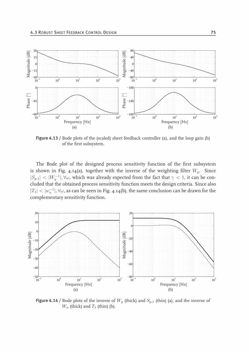
4.3 ROBUST SHEET FEEDBACK CONTROL DESIGN 75
10−1
100
101
102
103
−30
−15
0
15
30
10−1
100
101
102
103
−90
−45
0
Magnitude
[dB]
Phase
[]
Frequency [Hz](a)
10−1
100
101
102
103
−80
−40
0
40
80
10−1
100
101
102
103
−180
−140
−100
Magnitude
[dB]
Phase
[]
Frequency [Hz](b)
Figure 4.13 / Bode plots of the (scaled) sheet feedback controller (a), and the loop gain (b)of the first subsystem.
The Bode plot of the designed process sensitivity function of the first subsystemis shown in Fig. 4.14(a), together with the inverse of the weighting filter Wy. Since|Sp,1| < |W−1
y |, ∀ω, which was already expected from the fact that γ < 1, it can be con-cluded that the obtained process sensitivity function meets the design criteria. Since also|T1| < |w−1
u |, ∀ω, as can be seen in Fig. 4.14(b), the same conclusion can be drawn for thecomplementary sensitivity function.
10−1
100
101
102
103
−50
−40
−30
−20
−10
0
10
20
Magnitude
[dB]
Frequency [Hz](a)
10−1
100
101
102
103
−80
−60
−40
−20
0
20
Magnitude
[dB]
Frequency [Hz](b)
Figure 4.14 / Bode plots of the inverse of Wy (thick) and Sp,1 (thin) (a), and the inverse ofWu (thick) and T1 (thin) (b).
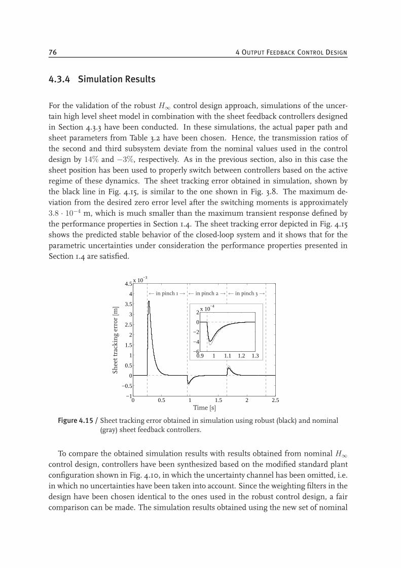
76 4 OUTPUT FEEDBACK CONTROL DESIGN
4.3.4 Simulation Results
For the validation of the robust H∞ control design approach, simulations of the uncer-tain high level sheet model in combination with the sheet feedback controllers designedin Section 4.3.3 have been conducted. In these simulations, the actual paper path andsheet parameters from Table 3.2 have been chosen. Hence, the transmission ratios ofthe second and third subsystem deviate from the nominal values used in the controldesign by 14% and −3%, respectively. As in the previous section, also in this case thesheet position has been used to properly switch between controllers based on the activeregime of these dynamics. The sheet tracking error obtained in simulation, shown bythe black line in Fig. 4.15, is similar to the one shown in Fig. 3.8. The maximum de-viation from the desired zero error level after the switching moments is approximately3.8 · 10−4 m, which is much smaller than the maximum transient response defined bythe performance properties in Section 1.4. The sheet tracking error depicted in Fig. 4.15shows the predicted stable behavior of the closed-loop system and it shows that for theparametric uncertainties under consideration the performance properties presented inSection 1.4 are satisfied.
0 0.5 1 1.5 2 2.5−1
−0.5
0
0.5
1
1.5
2
2.5
3
3.5
4
4.5x 10
−3
0.9 1 1.1 1.2 1.3−6
−4
−2
0
2x 10
−4
Time [s]
Sheettrackingerror[m
]
← in pinch 1→ ← in pinch 2→ ← in pinch 3→
Figure 4.15 / Sheet tracking error obtained in simulation using robust (black) and nominal(gray) sheet feedback controllers.
To compare the obtained simulation results with results obtained from nominal H∞control design, controllers have been synthesized based on the modified standard plantconfiguration shown in Fig. 4.10, in which the uncertainty channel has been omitted, i.e.in which no uncertainties have been taken into account. Since the weighting filters in thedesign have been chosen identical to the ones used in the robust control design, a faircomparison can be made. The simulation results obtained using the new set of nominal
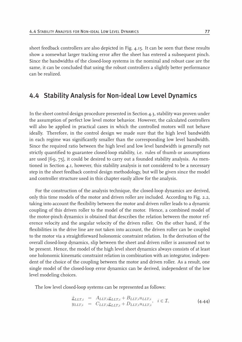
4.4 STABILITY ANALYSIS FOR NON-IDEAL LOW LEVEL DYNAMICS 77
sheet feedback controllers are also depicted in Fig. 4.15. It can be seen that these resultsshow a somewhat larger tracking error after the sheet has entered a subsequent pinch.Since the bandwidths of the closed-loop systems in the nominal and robust case are thesame, it can be concluded that using the robust controllers a slightly better performancecan be realized.
4.4 Stability Analysis for Non-ideal Low Level Dynamics
In the sheet control design procedure presented in Section 4.3, stability was proven underthe assumption of perfect low level motor behavior. However, the calculated controllerswill also be applied in practical cases in which the controlled motors will not behaveideally. Therefore, in the control design we made sure that the high level bandwidthin each regime was significantly smaller than the corresponding low level bandwidth.Since the required ratio between the high level and low level bandwidth is generally notstrictly quantified to guarantee closed-loop stability, i.e. rules of thumb or assumptionsare used [69, 75], it could be desired to carry out a founded stability analysis. As men-tioned in Section 4.1, however, this stability analysis is not considered to be a necessarystep in the sheet feedback control design methodology, but will be given since the modeland controller structure used in this chapter easily allow for the analysis.
For the construction of the analysis technique, the closed-loop dynamics are derived,only this time models of the motor and driven roller are included. According to Fig. 2.2,taking into account the flexibility between the motor and driven roller leads to a dynamiccoupling of this driven roller to the model of the motor. Hence, a combined model ofthe motor-pinch dynamics is obtained that describes the relation between the motor ref-erence velocity and the angular velocity of the driven roller. On the other hand, if theflexibilities in the drive line are not taken into account, the driven roller can be coupledto the motor via a straightforward holonomic constraint relation. In the derivation of theoverall closed-loop dynamics, slip between the sheet and driven roller is assumed not tobe present. Hence, the model of the high level sheet dynamics always consists of at leastone holonomic kinematic constraint relation in combination with an integrator, indepen-dent of the choice of the coupling between the motor and driven roller. As a result, onesingle model of the closed-loop error dynamics can be derived, independent of the lowlevel modeling choices.
The low level closed-loop systems can be represented as follows:
xLLT,i = ALLT,ixLLT,i +BLLT,iuLLT,iyLLT,i = CLLT,ixLLT,i +DLLT,iuLLT,i
, i ∈ I, (4.44)
78 4 OUTPUT FEEDBACK CONTROL DESIGN
with uLLT,i the reference velocity for motor Mi, calculated by the sheet feedback controllerof the i-th subsystem, and yLLT,i the i-th input of the high level sheet dynamics. Morespecifically, yLLT,i represents the actual velocity of motor Mi in case the flexibility betweenmotor and driven roller is neglected, or it represents the velocity of pinch i, in case theflexibility is taken into account. Furthermore,ALLT,i,BLLT,i, CLLT,i, andDLLT,i representthe state matrices, the input matrices, the output matrices, and the throughput matricesof the low level closed-loop systems.
The series connection of (4.44) and the model describing the high level sheet dynam-ics,
xs = BHLP,i
yLLT,1yLLT,2yLLT,3
for xs ∈ Xi, i ∈ I, (4.45)
yields the overall plant to be controlled by the high level sheet feedback controllers.In (4.45), BHLP,i is equal to Bi in (2.2) and (3.42) in case the flexibility between the motorand the driven roller is not taken into account in the modeling procedure. Otherwise,BHLP,i will only contain the radii of the driven rollers.
Given the model of the low level closed-loop systems (4.44), the model describing thehigh level sheet dynamics (4.45), and the robust H∞ feedback controllers representedby (4.9), the model of the overall closed-loop system can be derived. Given this model,the LMIs in (4.19) and (4.13), with Ai representing the state matrices of the model ofthe overall switched linear closed-loop system, can be used to check the stability of theswitched linear closed-loop dynamics. The results of the stability analysis in case of non-ideal low level dynamics will be presented in Section 6.3.1, after the motor dynamics havebeen identified and modeled, as described in Section 6.1.
A next step in the stability analysis would be to consider robust stability of the systemwith non-ideal low level dynamics, i.e. to include the uncertainty terms of the high levelsheet dynamics in the stability analysis. However, this extension will not be consideredhere and remains open for future research.
4.5 Evaluation
In this chapter, (robust)H∞ controllers have been designed for the basic paper path case-study. The main beneficial differences with respect to the approach presented in Chap-ter 3 are the following. First of all, robustness against parameter perturbations within aprespecified region is guaranteed in the controller synthesis, that, similar to Chapter 3,is carried out without taking into account the controlled motor dynamics. Hence, no
4.5 EVALUATION 79
a posteriori stability and performance analysis is needed. Secondly, the control designand the controller structure are independent of the sheet reference profile. Hence, ad-ditional dynamics, as for example high frequency roll-off, can be easily incorporated inthe controller. The third benefit is that using the weighting filters in the control design,bandwidth requirements and disturbance attenuation properties can be incorporated inthe controller design. Fourthly, in the approach presented in this chapter, no structure ofthe sheet feedback controllers has to be enforced to cope with possible jumps in xs and es,as the design process implicitly accounts for these discontinuities. Besides these benefits,some concerns are present with respect to the approach presented in the previous chapter,especially considering the use of the methodology in an industrial environment [73].
One of the concerns is that choosing the right parameter values for the weightingfilters is not straightforward. More specifically, in many cases iterations are requiredto achieve, for example, a desired value of γ < 1, stable controllers, and the desiredbandwidth, although the bandwidth resulting from the initial filter choice is likely to be inthe neighborhood of the desired one. Secondly, sensitivity for numerical ill-conditioningis relatively high. To reduce this sensitivity, scaling of the nominal model and weightsand transformation to balanced realizations can be applied [74]. Furthermore, care hasto be taken not to choose the dynamic ranges of the weighting filters too large, since thiscan result in numerical ill-conditioning of the resulting controller. A third concern is thatusing theH∞ control design approach, no pure integral action and roll-off can be realized.This is due to the fact that the weighting filters are chosen to be biproper and stable toprevent inserting a pole in ω = 0 in the augmented plant, that cannot be stabilized bythe controller. Hence, care has to be taken not to place the poles in (4.25) and (4.42) at afrequency that is too high, since this could result in steady state sheet tracking errors thatare too large.
Regarding the implementation of the controllers designed in this chapter, two disad-vantages with respect to the controllers presented in the previous chapter exist. First ofall, the controllers to be implemented are of 8-th order, which results in an increase incomputational effort on a CPU compared with the effort needed in case of the first ordercontrollers designed in Section 3.2.2.3 However, since the dynamics of the controllers weare interested in only consist of an integral action and a roll-off, reduction of the controllerorder might be possible, yielding second order controllers. The second disadvantage isthe fact that state information of the plant dynamics is needed in the implementation ofthe controller, since switching synchronously with the plant dynamics is required. Hence,the switching controllers do not result in robustness for possible deviations of the pinchlocations.
3When presenting the experimental results in Chapter 6, the computational effort needed for bothcontrollers will be analyzed.

80 4 OUTPUT FEEDBACK CONTROL DESIGN
Given the control design results presented in the Sections 3.2.2 and 4.3.3, an exper-imental validation of the two approaches can be conducted. To facilitate these experi-ments, an experimental paper path setup has been built, that will be discussed in thenext chapter.
CHAPTER FIVE
The Experimental Paper Path Setup
5.1 The Sheet Transportation Unit . . . . . . . . . . . . . . . . . . . . . . . 81
5.2 Sheet Position Measurement . . . . . . . . . . . . . . . . . . . . . . . . 83
5.1 The Sheet Transportation Unit
For the practical validation of the proposed control design approaches, an experimentalpaper path setup has been designed and built. Before designing the setup, a numberof requirements was formulated [82]. One important requirement in the design encom-passed the maximum achievable sheet velocity and acceleration, which were determinedto be 1 m/s and 10 m/s2 [15]. These requirements on the sheet motion profile in turnimpose requirements on the actuators driving the pinches. Another condition that had tobe taken into account in the design was the adaptability of the setup, such that controllerdesigns for a wide range of case-studies could be experimentally validated. This conditionwas imposed considering the future extension of the basic paper path case-study to realprinter paper path case-studies. For example, it had to be possible to change the locationof pinches, such that the sheet can be driven by more than one pinch. Furthermore,grouping pinches into sections driven by a single motor had to be possible. In this case,an industrial paper path as the one shown in Fig. 1.3 could be mimicked.
Based on the requirements, the experimental paper path setup depicted in Fig. 5.1 hasbeen realized. As can be seen in the figure, the setup consists of a PIM and a paperpath with five pinches. Whereas in real printer paper paths aluminium plates are usedto guide the sheets through the paper path, in the experimental setup thin steel wires
81
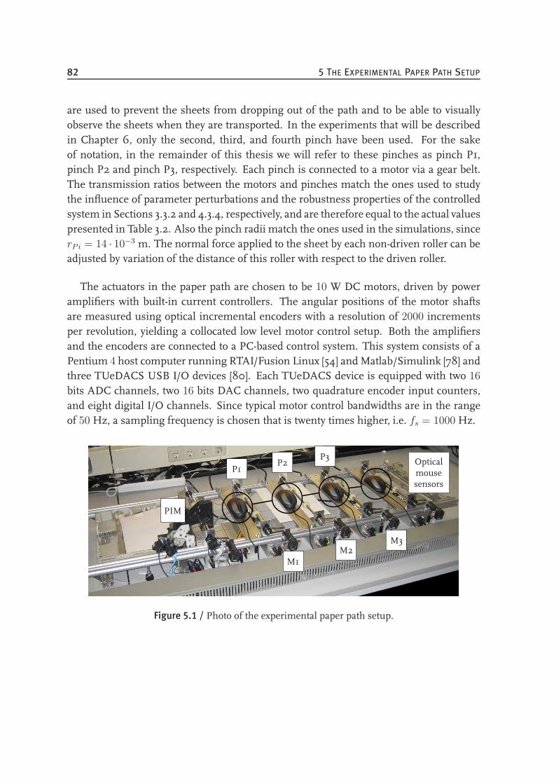
82 5 THE EXPERIMENTAL PAPER PATH SETUP
are used to prevent the sheets from dropping out of the path and to be able to visuallyobserve the sheets when they are transported. In the experiments that will be describedin Chapter 6, only the second, third, and fourth pinch have been used. For the sakeof notation, in the remainder of this thesis we will refer to these pinches as pinch P1,pinch P2 and pinch P3, respectively. Each pinch is connected to a motor via a gear belt.The transmission ratios between the motors and pinches match the ones used to studythe influence of parameter perturbations and the robustness properties of the controlledsystem in Sections 3.3.2 and 4.3.4, respectively, and are therefore equal to the actual valuespresented in Table 3.2. Also the pinch radii match the ones used in the simulations, sincerPi = 14 · 10−3 m. The normal force applied to the sheet by each non-driven roller can beadjusted by variation of the distance of this roller with respect to the driven roller.
The actuators in the paper path are chosen to be 10 W DC motors, driven by poweramplifiers with built-in current controllers. The angular positions of the motor shaftsare measured using optical incremental encoders with a resolution of 2000 incrementsper revolution, yielding a collocated low level motor control setup. Both the amplifiersand the encoders are connected to a PC-based control system. This system consists of aPentium 4 host computer running RTAI/Fusion Linux [54] andMatlab/Simulink [78] andthree TUeDACS USB I/O devices [80]. Each TUeDACS device is equipped with two 16
bits ADC channels, two 16 bits DAC channels, two quadrature encoder input counters,and eight digital I/O channels. Since typical motor control bandwidths are in the rangeof 50 Hz, a sampling frequency is chosen that is twenty times higher, i.e. fs = 1000 Hz.
P1P2
P3
M1M2
M3
PIM
Opticalmousesensors
Figure 5.1 / Photo of the experimental paper path setup.
5.2 SHEET POSITION MEASUREMENT 83
5.2 Sheet Position Measurement
5.2.1 Sensor Selection
To be able to implement the sheet feedback controllers in practice and to verify the ro-bustness of the closed-loop system, the sheet position must be known at all time instants.Since our practical setup allows for a simple direct measurement of the state and outputof the sheet flow model, i.e. the sheet position, no observer will be needed. As defined inSection 1.4, themaximum steady state sheet tracking error is 5·10−4 m. From this we pro-pose a resolution of 1 · 10−4 m for the, preferably absolute and contactless, sheet positionsensor. Two examples of commercially available absolute contactless position sensors aremeasuring light beams and photo-electric slot sensors [2]. Both systems use multiplesmall light beams that are interrupted when a sheet passes. However, as their resolutionis 2.5 · 10−3 m and 3 · 10−4 m, respectively, they do not have the required resolution.
As an alternative for absolute position measurement systems, relative displacementsensors could be used. An example of a relative displacement sensor is the sensor usedin optical mouse devices. These sensors are relatively cheap, and by placing them at adistance which is a little smaller than the sheet length, only a limited number of sensorsis needed. Furthermore, today’s mouse sensors have a very good resolution. An exampleof such sensor is the Agilent ADNS-6010 optical laser mouse sensor, supplied by AvagoTechnologies [1], which can be found in the Logitech G5 Laser mouse [51]. This sensor issuitable for high speed motion detection, with a maximal velocity and acceleration up to1.14 m/s and 196 m/s2, respectively. The maximum sensor resolution is 2000 counts perinch (cpi), which corresponds to 12.7 · 10−6 m per count. Since these specifications meetthe requirements, the mouse sensors are chosen to act as a sheet position measurementsystem. However, care has to be taken when mounting the sensors onto the paper path,since the specifications given in the sensor’s data sheet depend on several environmentalproperties, of which the distance between the sensor lens and the sheet surface is mostcrucial. The recommended range for this distance is 2.1 · 10−3 − 2.7 · 10−3 m.
The working principle of the optical mouse sensor is schematically depicted in Fig.5.2,which is taken from [1]. Light from a Vertical Cavity Surface Emitting Laser (VCSEL),represented by the thick gray line, is transported through a lens to illuminate the surfacethe mouse is working on. The reflected light is projected onto the mouse sensor, againvia the lens. The sensor contains an Image Acquisition System (IAS), a Digital SignalProcessor (DSP), and a serial port. The IAS acquires images, which are processed by theDSP. By comparing two sequentially taken images of the surface, the direction and thedistance of the motion are determined, after which the relative displacement values in
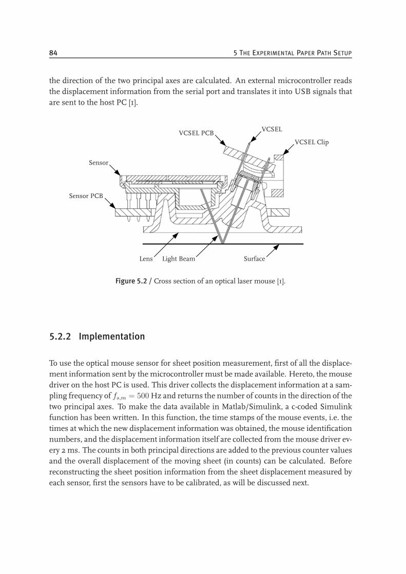
84 5 THE EXPERIMENTAL PAPER PATH SETUP
the direction of the two principal axes are calculated. An external microcontroller readsthe displacement information from the serial port and translates it into USB signals thatare sent to the host PC [1].
Sensor
Sensor PCB
Lens Light Beam Surface
VCSEL Clip
VCSELVCSEL PCB
Figure 5.2 / Cross section of an optical laser mouse [1].
5.2.2 Implementation
To use the optical mouse sensor for sheet position measurement, first of all the displace-ment information sent by themicrocontrollermust bemade available. Hereto, themousedriver on the host PC is used. This driver collects the displacement information at a sam-pling frequency of fs,m = 500Hz and returns the number of counts in the direction of thetwo principal axes. To make the data available in Matlab/Simulink, a c-coded Simulinkfunction has been written. In this function, the time stamps of the mouse events, i.e. thetimes at which the new displacement information was obtained, the mouse identificationnumbers, and the displacement information itself are collected from the mouse driver ev-ery 2 ms. The counts in both principal directions are added to the previous counter valuesand the overall displacement of the moving sheet (in counts) can be calculated. Beforereconstructing the sheet position information from the sheet displacement measured byeach sensor, first the sensors have to be calibrated, as will be discussed next.
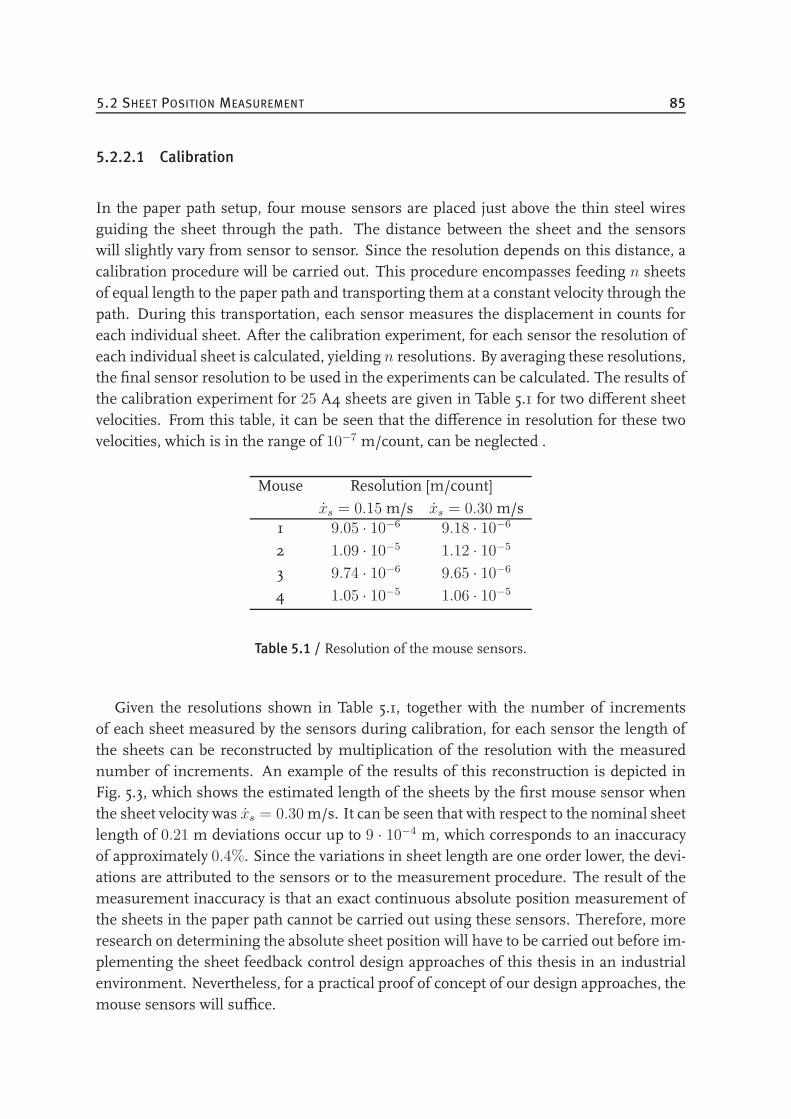
5.2 SHEET POSITION MEASUREMENT 85
5.2.2.1 Calibration
In the paper path setup, four mouse sensors are placed just above the thin steel wiresguiding the sheet through the path. The distance between the sheet and the sensorswill slightly vary from sensor to sensor. Since the resolution depends on this distance, acalibration procedure will be carried out. This procedure encompasses feeding n sheetsof equal length to the paper path and transporting them at a constant velocity through thepath. During this transportation, each sensor measures the displacement in counts foreach individual sheet. After the calibration experiment, for each sensor the resolution ofeach individual sheet is calculated, yielding n resolutions. By averaging these resolutions,the final sensor resolution to be used in the experiments can be calculated. The results ofthe calibration experiment for 25 A4 sheets are given in Table 5.1 for two different sheetvelocities. From this table, it can be seen that the difference in resolution for these twovelocities, which is in the range of 10−7 m/count, can be neglected .
Mouse Resolution [m/count]
xs = 0.15 m/s xs = 0.30 m/s1 9.05 · 10−6 9.18 · 10−6
2 1.09 · 10−5 1.12 · 10−5
3 9.74 · 10−6 9.65 · 10−6
4 1.05 · 10−5 1.06 · 10−5
Table 5.1 / Resolution of the mouse sensors.
Given the resolutions shown in Table 5.1, together with the number of incrementsof each sheet measured by the sensors during calibration, for each sensor the length ofthe sheets can be reconstructed by multiplication of the resolution with the measurednumber of increments. An example of the results of this reconstruction is depicted inFig. 5.3, which shows the estimated length of the sheets by the first mouse sensor whenthe sheet velocity was xs = 0.30 m/s. It can be seen that with respect to the nominal sheetlength of 0.21 m deviations occur up to 9 · 10−4 m, which corresponds to an inaccuracyof approximately 0.4%. Since the variations in sheet length are one order lower, the devi-ations are attributed to the sensors or to the measurement procedure. The result of themeasurement inaccuracy is that an exact continuous absolute position measurement ofthe sheets in the paper path cannot be carried out using these sensors. Therefore, moreresearch on determining the absolute sheet position will have to be carried out before im-plementing the sheet feedback control design approaches of this thesis in an industrialenvironment. Nevertheless, for a practical proof of concept of our design approaches, themouse sensors will suffice.
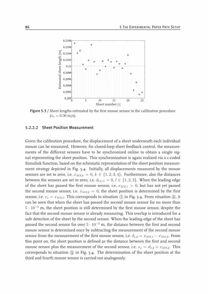
86 5 THE EXPERIMENTAL PAPER PATH SETUP
0 5 10 15 20 250.209
0.2092
0.2094
0.2096
0.2098
0.21
0.2102
0.2104
0.2106
0.2108
Sheet number [-]
Estim
ated
sheetlen
gth[m
]
Figure 5.3 / Sheet lengths estimated by the first mouse sensor in the calibration procedure(xs = 0.30 m/s).
5.2.2.2 Sheet Position Measurement
Given the calibration procedure, the displacement of a sheet underneath each individualmouse can be measured. However, for closed-loop sheet feedback control, the measure-ments of the different sensors have to be synchronized online to obtain a single sig-nal representing the sheet position. This synchronization is again realized via a c-codedSimulink function, based on the schematic representation of the sheet position measure-ment strategy depicted in Fig. 5.4. Initially, all displacements measured by the mousesensors are set to zero, i.e. xMS,k = 0, k ∈ 1, 2, 3, 4. Furthermore, also the distancesbetween the sensors are set to zero, i.e. dl,l+1 = 0, l ∈ 1, 2, 3. When the leading edgeof the sheet has passed the first mouse sensor, i.e. xMS,1 > 0, but has not yet passedthe second mouse sensor, i.e. xMS,2 = 0, the sheet position is determined by the firstsensor, i.e. xs = xMS,1. This corresponds to situation 1© in Fig. 5.4. From situation 2©, itcan be seen that when the sheet has passed the second mouse sensor for no more than5 · 10−3 m, the sheet position is still determined by the first mouse sensor, despite thefact that the second mouse sensor is already measuring. This overlap is introduced for asafe detection of the sheet by the second sensor. When the leading edge of the sheet haspassed the second sensor for over 5 · 10−3 m, the distance between the first and secondmouse sensor is determined once by subtracting the measurement of the second mousesensor from the measurement of the first mouse sensor, i.e. d1,2 = xMS,1 − xMS,2. Fromthis point on, the sheet position is defined as the distance between the first and secondmouse sensor plus the measurement of the second sensor, i.e. xs = d1,2 + xMS,2. Thiscorresponds to situation 3© in Fig. 5.4. The determination of the sheet position at thethird and fourth mouse sensor is carried out analogously.
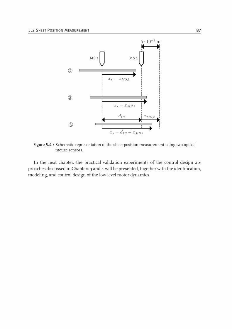
5.2 SHEET POSITION MEASUREMENT 87
5 · 10−3 m
xs = xMS,1
xs = xMS,1
d1,2 xMS,2
xs = d1,2 + xMS,2
1©
2©
3©
MS 1 MS 2
Figure 5.4 / Schematic representation of the sheet position measurement using two opticalmouse sensors.
In the next chapter, the practical validation experiments of the control design ap-proaches discussed in Chapters 3 and 4 will be presented, together with the identification,modeling, and control design of the low level motor dynamics.

88
CHAPTER SIX
Experimental Results
6.1 Low Level Motor Dynamics . . . . . . . . . . . . . . . . . . . . . . . . . 89
6.2 Experimental Validation Results - The State Feedback Control Approach 93
6.3 Experimental Validation Results - The Output Feedback Control Approach100
6.1 Low Level Motor Dynamics
In this chapter the practical validation experiments of the control design approaches pre-sented in Chapters 3 and 4 will be described, together with the comparison with thecorresponding simulation results. However, first identification and control design of thelow level motor dynamics will be discussed, after which the models of the closed-loopmotor dynamics, needed for carrying out the stability analysis of the complete system,will be derived.
In the design procedures of the sheet feedback controllers, perfect tracking behaviorof the controlled motors was assumed, i.e. the motor control loops were assumed to havean infinite bandwidth. Furthermore, we assumed an infinitely stiff coupling betweenthe motors and the pinches. In the experimental setup, however, these assumptions donot hold. The digital implementation of the controllers will cause a delay in the controlloop, that will limit the attainable bandwidth. Another limitation results from the rubberbelt that connects the motor with driven roller of the pinch. Since this belt has a finitestiffness, flexibilities will be present in the system that can limit the attainable bandwidthas well.
89
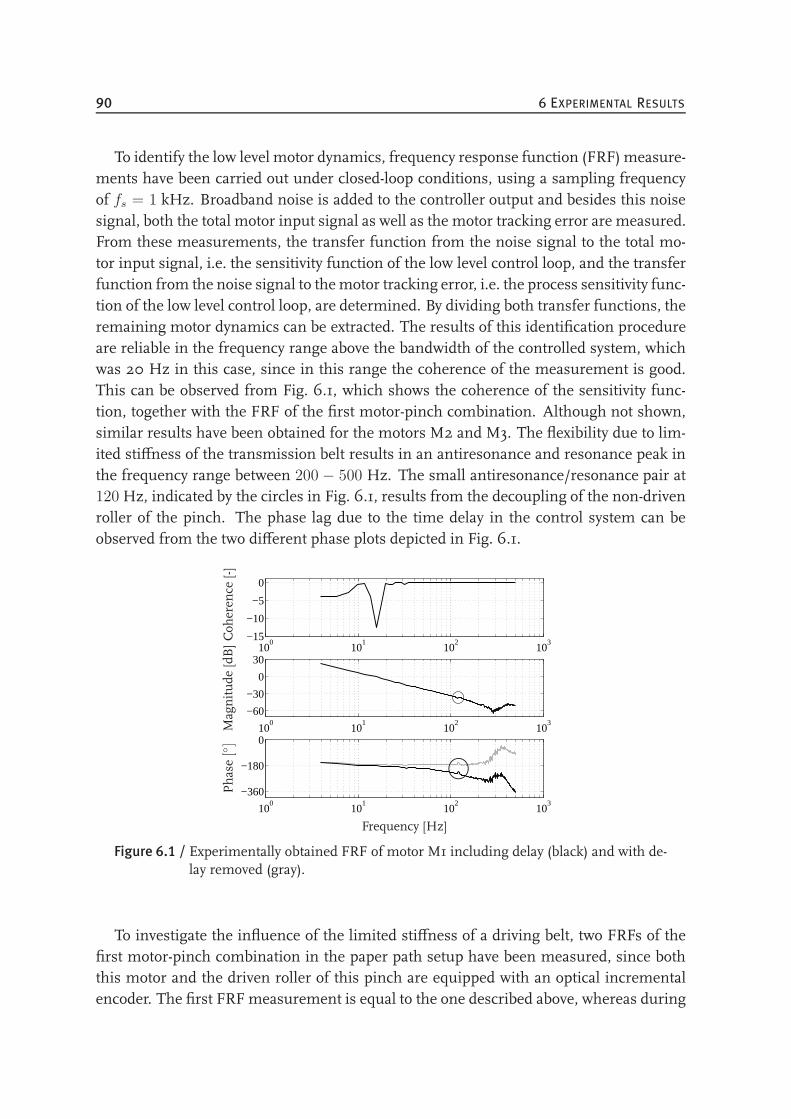
90 6 EXPERIMENTAL RESULTS
To identify the low level motor dynamics, frequency response function (FRF) measure-ments have been carried out under closed-loop conditions, using a sampling frequencyof fs = 1 kHz. Broadband noise is added to the controller output and besides this noisesignal, both the total motor input signal as well as the motor tracking error are measured.From these measurements, the transfer function from the noise signal to the total mo-tor input signal, i.e. the sensitivity function of the low level control loop, and the transferfunction from the noise signal to themotor tracking error, i.e. the process sensitivity func-tion of the low level control loop, are determined. By dividing both transfer functions, theremaining motor dynamics can be extracted. The results of this identification procedureare reliable in the frequency range above the bandwidth of the controlled system, whichwas 20 Hz in this case, since in this range the coherence of the measurement is good.This can be observed from Fig. 6.1, which shows the coherence of the sensitivity func-tion, together with the FRF of the first motor-pinch combination. Although not shown,similar results have been obtained for the motors M2 and M3. The flexibility due to lim-ited stiffness of the transmission belt results in an antiresonance and resonance peak inthe frequency range between 200 − 500 Hz. The small antiresonance/resonance pair at120 Hz, indicated by the circles in Fig. 6.1, results from the decoupling of the non-drivenroller of the pinch. The phase lag due to the time delay in the control system can beobserved from the two different phase plots depicted in Fig. 6.1.
100
101
102
103
−15
−10
−5
0
100
101
102
103
−60
−30
0
30
100
101
102
103
−360
−180
0
Coh
eren
ce[-]
Magnitude
[dB]
Phase
[]
Frequency [Hz]
©
©
Figure 6.1 / Experimentally obtained FRF of motor M1 including delay (black) and with de-lay removed (gray).
To investigate the influence of the limited stiffness of a driving belt, two FRFs of thefirst motor-pinch combination in the paper path setup have been measured, since boththis motor and the driven roller of this pinch are equipped with an optical incrementalencoder. The first FRF measurement is equal to the one described above, whereas during
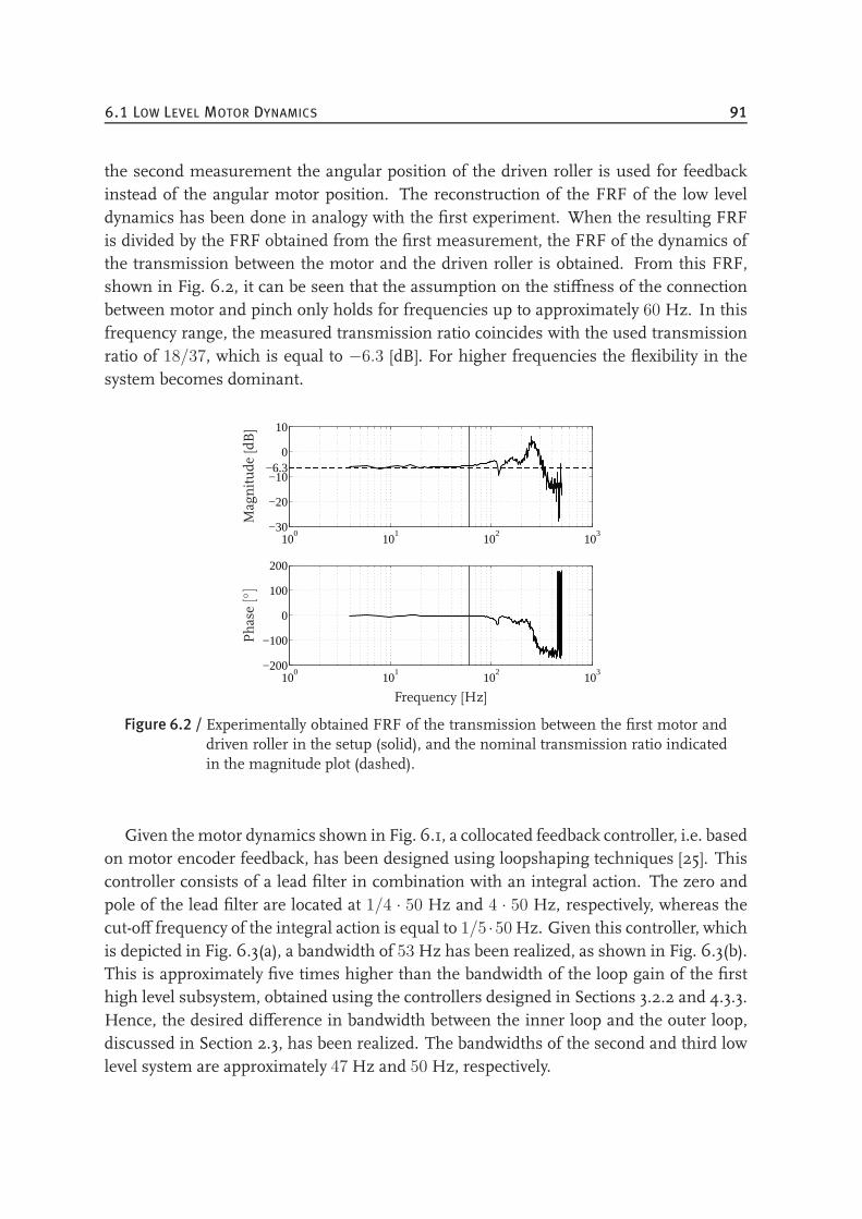
6.1 LOW LEVEL MOTOR DYNAMICS 91
the second measurement the angular position of the driven roller is used for feedbackinstead of the angular motor position. The reconstruction of the FRF of the low leveldynamics has been done in analogy with the first experiment. When the resulting FRFis divided by the FRF obtained from the first measurement, the FRF of the dynamics ofthe transmission between the motor and the driven roller is obtained. From this FRF,shown in Fig. 6.2, it can be seen that the assumption on the stiffness of the connectionbetween motor and pinch only holds for frequencies up to approximately 60 Hz. In thisfrequency range, the measured transmission ratio coincides with the used transmissionratio of 18/37, which is equal to −6.3 [dB]. For higher frequencies the flexibility in thesystem becomes dominant.
100
101
102
103
−30
−20
−10−6.3
0
10
100
101
102
103
−200
−100
0
100
200
Magnitude
[dB]
Phase
[]
Frequency [Hz]
Figure 6.2 / Experimentally obtained FRF of the transmission between the first motor anddriven roller in the setup (solid), and the nominal transmission ratio indicatedin the magnitude plot (dashed).
Given themotor dynamics shown in Fig. 6.1, a collocated feedback controller, i.e. basedon motor encoder feedback, has been designed using loopshaping techniques [25]. Thiscontroller consists of a lead filter in combination with an integral action. The zero andpole of the lead filter are located at 1/4 · 50 Hz and 4 · 50 Hz, respectively, whereas thecut-off frequency of the integral action is equal to 1/5 ·50Hz. Given this controller, whichis depicted in Fig. 6.3(a), a bandwidth of 53 Hz has been realized, as shown in Fig. 6.3(b).This is approximately five times higher than the bandwidth of the loop gain of the firsthigh level subsystem, obtained using the controllers designed in Sections 3.2.2 and 4.3.3.Hence, the desired difference in bandwidth between the inner loop and the outer loop,discussed in Section 2.3, has been realized. The bandwidths of the second and third lowlevel system are approximately 47 Hz and 50 Hz, respectively.
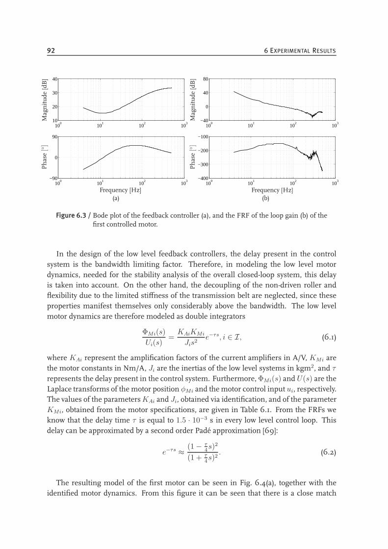
92 6 EXPERIMENTAL RESULTS
100
101
102
103
10
20
30
40
100
101
102
103
−90
0
90
Magnitude
[dB]
Phase
[]
Frequency [Hz](a)
100
101
102
103
−40
0
40
80
100
101
102
103
−400
−300
−200
−100
Magnitude
[dB]
Phase
[]
Frequency [Hz](b)
Figure 6.3 / Bode plot of the feedback controller (a), and the FRF of the loop gain (b) of thefirst controlled motor.
In the design of the low level feedback controllers, the delay present in the controlsystem is the bandwidth limiting factor. Therefore, in modeling the low level motordynamics, needed for the stability analysis of the overall closed-loop system, this delayis taken into account. On the other hand, the decoupling of the non-driven roller andflexibility due to the limited stiffness of the transmission belt are neglected, since theseproperties manifest themselves only considerably above the bandwidth. The low levelmotor dynamics are therefore modeled as double integrators
ΦMi(s)
Ui(s)=KAiKMi
Jis2e−τs, i ∈ I, (6.1)
where KAi represent the amplification factors of the current amplifiers in A/V, KMi arethe motor constants in Nm/A, Ji are the inertias of the low level systems in kgm2, and τrepresents the delay present in the control system. Furthermore,ΦMi(s) and U(s) are theLaplace transforms of the motor position φMi and themotor control input ui, respectively.The values of the parametersKAi and Ji, obtained via identification, and of the parameterKMi, obtained from the motor specifications, are given in Table 6.1. From the FRFs weknow that the delay time τ is equal to 1.5 · 10−3 s in every low level control loop. Thisdelay can be approximated by a second order Padé approximation [69]:
e−τs ≈(1 − τ
4s)2
(1 + τ4s)2
. (6.2)
The resulting model of the first motor can be seen in Fig. 6.4(a), together with theidentified motor dynamics. From this figure it can be seen that there is a close match
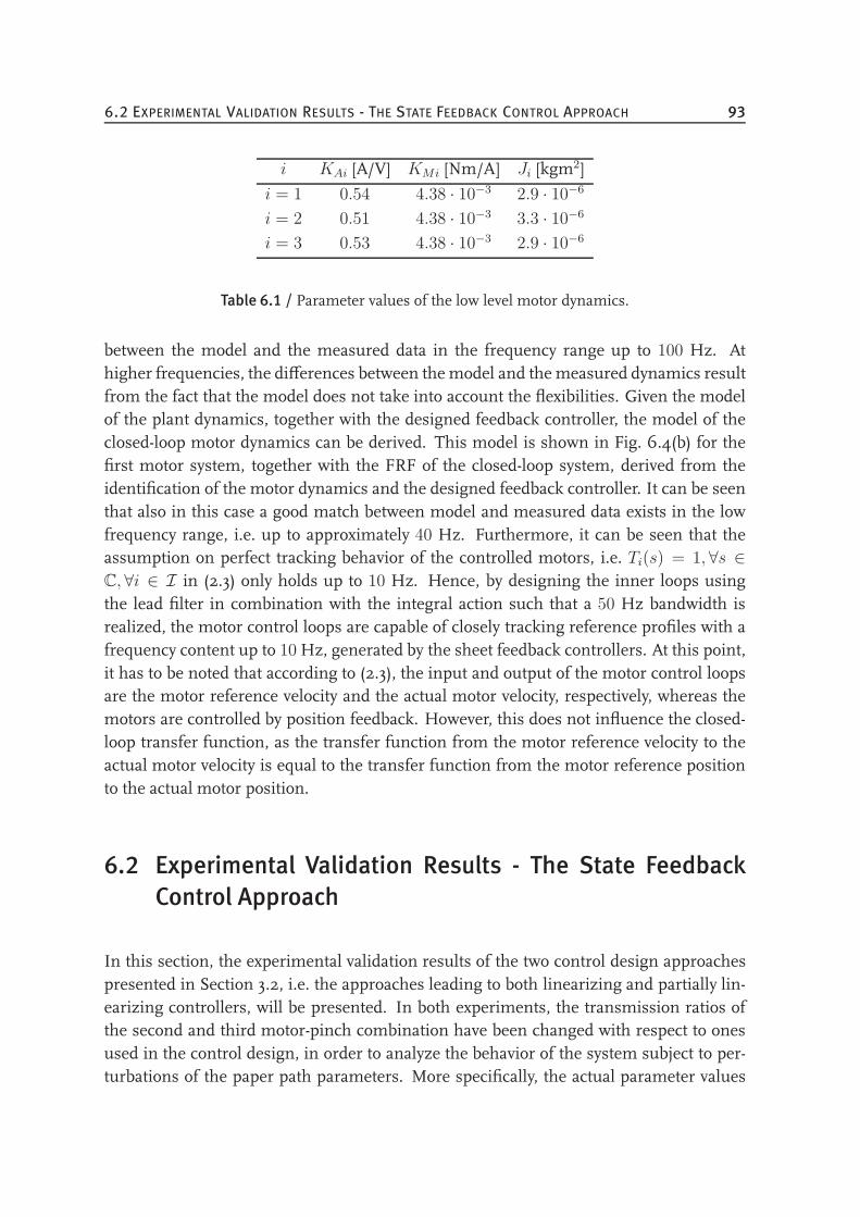
6.2 EXPERIMENTAL VALIDATION RESULTS - THE STATE FEEDBACK CONTROL APPROACH 93
i KAi [A/V] KMi [Nm/A] Ji [kgm2]
i = 1 0.54 4.38 · 10−3 2.9 · 10−6
i = 2 0.51 4.38 · 10−3 3.3 · 10−6
i = 3 0.53 4.38 · 10−3 2.9 · 10−6
Table 6.1 / Parameter values of the low level motor dynamics.
between the model and the measured data in the frequency range up to 100 Hz. Athigher frequencies, the differences between themodel and themeasured dynamics resultfrom the fact that the model does not take into account the flexibilities. Given the modelof the plant dynamics, together with the designed feedback controller, the model of theclosed-loop motor dynamics can be derived. This model is shown in Fig. 6.4(b) for thefirst motor system, together with the FRF of the closed-loop system, derived from theidentification of the motor dynamics and the designed feedback controller. It can be seenthat also in this case a good match between model and measured data exists in the lowfrequency range, i.e. up to approximately 40 Hz. Furthermore, it can be seen that theassumption on perfect tracking behavior of the controlled motors, i.e. Ti(s) = 1, ∀s ∈
C, ∀i ∈ I in (2.3) only holds up to 10 Hz. Hence, by designing the inner loops usingthe lead filter in combination with the integral action such that a 50 Hz bandwidth isrealized, the motor control loops are capable of closely tracking reference profiles with afrequency content up to 10 Hz, generated by the sheet feedback controllers. At this point,it has to be noted that according to (2.3), the input and output of the motor control loopsare the motor reference velocity and the actual motor velocity, respectively, whereas themotors are controlled by position feedback. However, this does not influence the closed-loop transfer function, as the transfer function from the motor reference velocity to theactual motor velocity is equal to the transfer function from the motor reference positionto the actual motor position.
6.2 Experimental Validation Results - The State Feedback
Control Approach
In this section, the experimental validation results of the two control design approachespresented in Section 3.2, i.e. the approaches leading to both linearizing and partially lin-earizing controllers, will be presented. In both experiments, the transmission ratios ofthe second and third motor-pinch combination have been changed with respect to onesused in the control design, in order to analyze the behavior of the system subject to per-turbations of the paper path parameters. More specifically, the actual parameter values
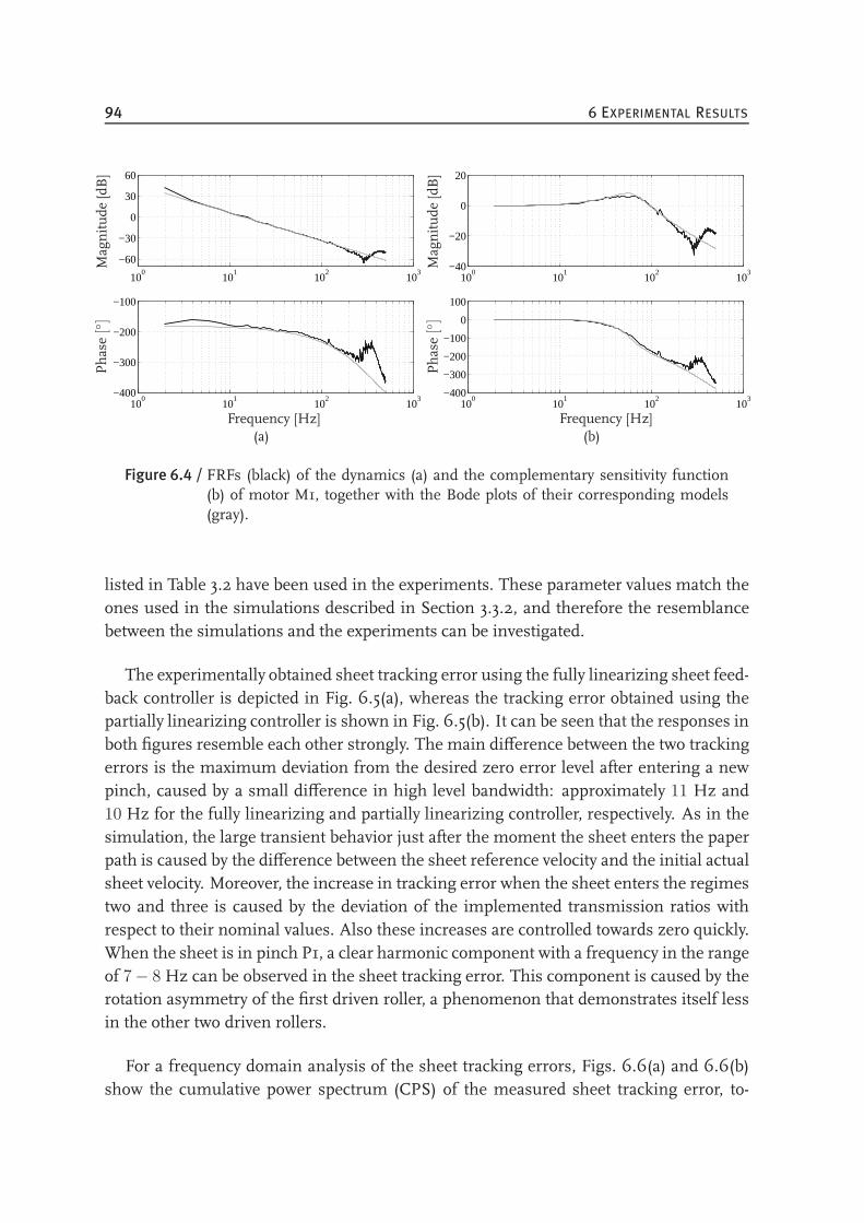
94 6 EXPERIMENTAL RESULTS
100
101
102
103
−60
−30
0
30
60
100
101
102
103
−400
−300
−200
−100
Magnitude
[dB]
Phase
[]
Frequency [Hz](a)
100
101
102
103
−40
−20
0
20
100
101
102
103
−400
−300
−200
−100
0
100
Magnitude
[dB]
Phase
[]
Frequency [Hz](b)
Figure 6.4 / FRFs (black) of the dynamics (a) and the complementary sensitivity function(b) of motor M1, together with the Bode plots of their corresponding models(gray).
listed in Table 3.2 have been used in the experiments. These parameter values match theones used in the simulations described in Section 3.3.2, and therefore the resemblancebetween the simulations and the experiments can be investigated.
The experimentally obtained sheet tracking error using the fully linearizing sheet feed-back controller is depicted in Fig. 6.5(a), whereas the tracking error obtained using thepartially linearizing controller is shown in Fig. 6.5(b). It can be seen that the responses inboth figures resemble each other strongly. The main difference between the two trackingerrors is the maximum deviation from the desired zero error level after entering a newpinch, caused by a small difference in high level bandwidth: approximately 11 Hz and10 Hz for the fully linearizing and partially linearizing controller, respectively. As in thesimulation, the large transient behavior just after the moment the sheet enters the paperpath is caused by the difference between the sheet reference velocity and the initial actualsheet velocity. Moreover, the increase in tracking error when the sheet enters the regimestwo and three is caused by the deviation of the implemented transmission ratios withrespect to their nominal values. Also these increases are controlled towards zero quickly.When the sheet is in pinch P1, a clear harmonic component with a frequency in the rangeof 7− 8 Hz can be observed in the sheet tracking error. This component is caused by therotation asymmetry of the first driven roller, a phenomenon that demonstrates itself lessin the other two driven rollers.
For a frequency domain analysis of the sheet tracking errors, Figs. 6.6(a) and 6.6(b)show the cumulative power spectrum (CPS) of the measured sheet tracking error, to-
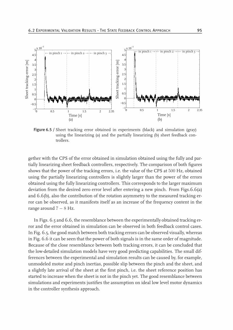
6.2 EXPERIMENTAL VALIDATION RESULTS - THE STATE FEEDBACK CONTROL APPROACH 95
0 0.5 1 1.5 2 2.35−1
−0.5
0
0.5
1
1.5
2
2.5
3
3.5
4
4.5
5x 10
−3
Time [s]
Sheettrackingerror[m
]
← in pinch 1→← in pinch 2→← in pinch 3→
(a)
0 0.5 1 1.5 2 2.35−1
−0.5
0
0.5
1
1.5
2
2.5
3
3.5
4
4.5
5x 10
−3
Time [s]Sheettrackingerror[m
]
← in pinch 1→← in pinch 2→← in pinch 3→
(b)
Figure 6.5 / Sheet tracking error obtained in experiments (black) and simulation (gray)using the linearizing (a) and the partially linearizing (b) sheet feedback con-trollers.
gether with the CPS of the error obtained in simulation obtained using the fully and par-tially linearizing sheet feedback controllers, respectively. The comparison of both figuresshows that the power of the tracking errors, i.e. the value of the CPS at 500 Hz, obtainedusing the partially linearizing controllers is slightly larger than the power of the errorsobtained using the fully linearizing controllers. This corresponds to the larger maximumdeviation from the desired zero error level after entering a new pinch. From Figs.6.6(a)and 6.6(b), also the contribution of the rotation asymmetry to the measured tracking er-ror can be observed, as it manifests itself as an increase of the frequency content in therange around 7 − 8 Hz.
In Figs. 6.5 and 6.6, the resemblance between the experimentally obtained tracking er-ror and the error obtained in simulation can be observed in both feedback control cases.In Fig. 6.5, the goodmatch between both tracking errors can be observed visually, whereasin Fig. 6.6 it can be seen that the power of both signals is in the same order of magnitude.Because of the close resemblance between both tracking errors, it can be concluded thatthe low-detailed simulation models have very good predicting capabilities. The small dif-ferences between the experimental and simulation results can be caused by, for example,unmodeled motor and pinch inertias, possible slip between the pinch and the sheet, anda slightly late arrival of the sheet at the first pinch, i.e. the sheet reference position hasstarted to increase when the sheet is not in the pinch yet. The good resemblance betweensimulations and experiments justifies the assumption on ideal low level motor dynamicsin the controller synthesis approach.
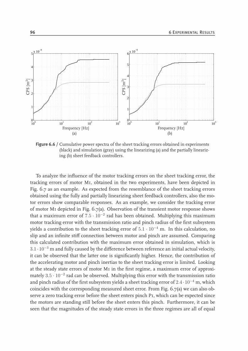
96 6 EXPERIMENTAL RESULTS
100
101
102
103
0
1
2
3
4
5x 10
−8
Frequency [Hz]
CPS[m
2]
(a)
100
101
102
103
0
1
2
3
4
5
6x 10
−8
Frequency [Hz]CPS[m
2]
(b)
Figure 6.6 / Cumulative power spectra of the sheet tracking errors obtained in experiments(black) and simulation (gray) using the linearizing (a) and the partially lineariz-ing (b) sheet feedback controllers.
To analyze the influence of the motor tracking errors on the sheet tracking error, thetracking errors of motor M1, obtained in the two experiments, have been depicted inFig. 6.7 as an example. As expected from the resemblance of the sheet tracking errorsobtained using the fully and partially linearizing sheet feedback controllers, also the mo-tor errors show comparable responses. As an example, we consider the tracking errorof motor M1 depicted in Fig. 6.7(a). Observation of the transient motor response showsthat a maximum error of 7.5 · 10−2 rad has been obtained. Multiplying this maximummotor tracking error with the transmission ratio and pinch radius of the first subsystemyields a contribution to the sheet tracking error of 5.1 · 10−4 m. In this calculation, noslip and an infinite stiff connection between motor and pinch are assumed. Comparingthis calculated contribution with the maximum error obtained in simulation, which is3.1 ·10−3 m and fully caused by the difference between reference an initial actual velocity,it can be observed that the latter one is significantly higher. Hence, the contribution ofthe accelerating motor and pinch inertias to the sheet tracking error is limited. Lookingat the steady state errors of motor M1 in the first regime, a maximum error of approxi-mately 3.5 · 10−2 rad can be observed. Multiplying this error with the transmission ratioand pinch radius of the first subsystem yields a sheet tracking error of 2.4 ·10−4 m, whichcoincides with the corresponding measured sheet error. From Fig. 6.7(a) we can also ob-serve a zero tracking error before the sheet enters pinch P1, which can be expected sincethe motors are standing still before the sheet enters this pinch. Furthermore, it can beseen that the magnitudes of the steady state errors in the three regimes are all of equal
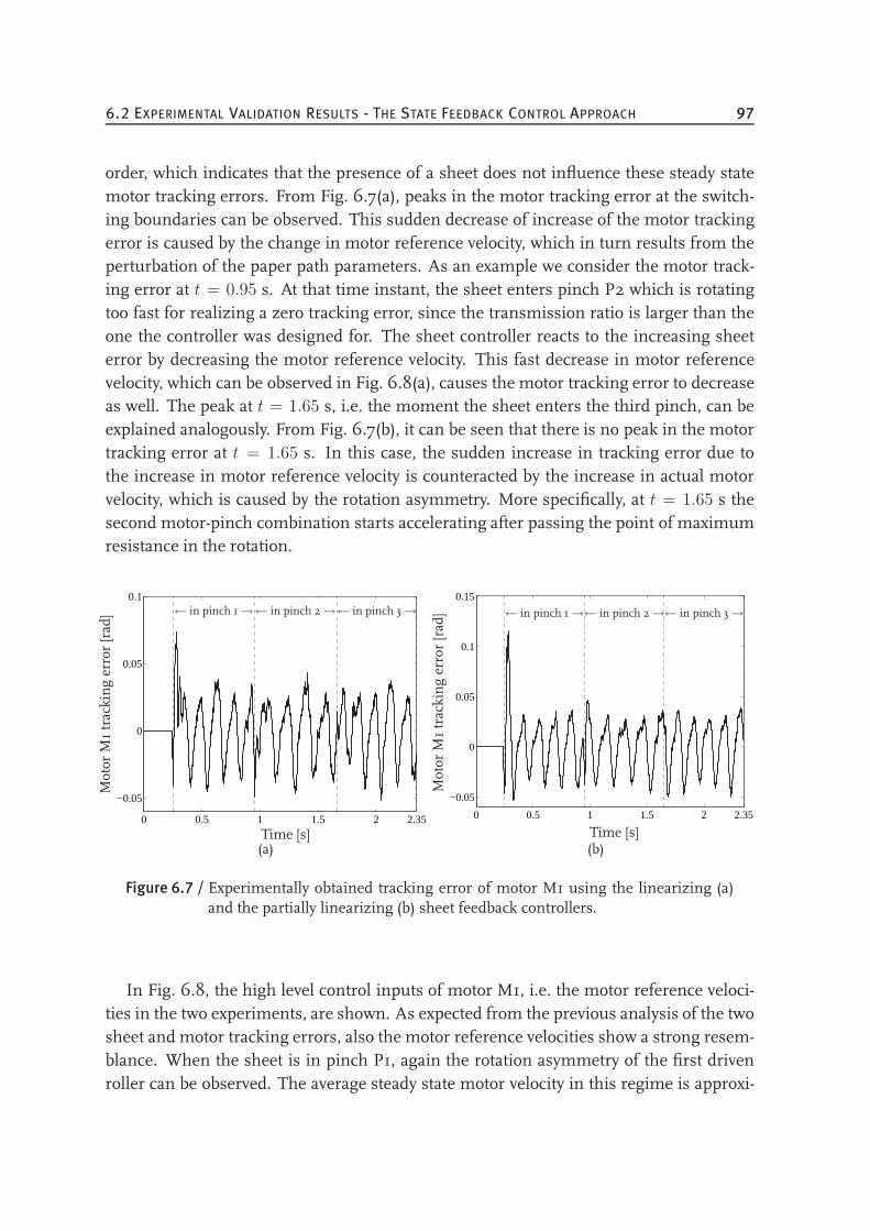
6.2 EXPERIMENTAL VALIDATION RESULTS - THE STATE FEEDBACK CONTROL APPROACH 97
order, which indicates that the presence of a sheet does not influence these steady statemotor tracking errors. From Fig. 6.7(a), peaks in the motor tracking error at the switch-ing boundaries can be observed. This sudden decrease of increase of the motor trackingerror is caused by the change in motor reference velocity, which in turn results from theperturbation of the paper path parameters. As an example we consider the motor track-ing error at t = 0.95 s. At that time instant, the sheet enters pinch P2 which is rotatingtoo fast for realizing a zero tracking error, since the transmission ratio is larger than theone the controller was designed for. The sheet controller reacts to the increasing sheeterror by decreasing the motor reference velocity. This fast decrease in motor referencevelocity, which can be observed in Fig. 6.8(a), causes the motor tracking error to decreaseas well. The peak at t = 1.65 s, i.e. the moment the sheet enters the third pinch, can beexplained analogously. From Fig. 6.7(b), it can be seen that there is no peak in the motortracking error at t = 1.65 s. In this case, the sudden increase in tracking error due tothe increase in motor reference velocity is counteracted by the increase in actual motorvelocity, which is caused by the rotation asymmetry. More specifically, at t = 1.65 s thesecond motor-pinch combination starts accelerating after passing the point of maximumresistance in the rotation.
0 0.5 1 1.5 2 2.35
−0.05
0
0.05
0.1
Time [s]
Motor
M1trackingerror[rad] ← in pinch 1→← in pinch 2→← in pinch 3→
(a)
0 0.5 1 1.5 2 2.35
−0.05
0
0.05
0.1
0.15
Time [s]
Motor
M1trackingerror[rad] ← in pinch 1→← in pinch 2→← in pinch 3→
(b)
Figure 6.7 / Experimentally obtained tracking error of motor M1 using the linearizing (a)and the partially linearizing (b) sheet feedback controllers.
In Fig. 6.8, the high level control inputs of motor M1, i.e. the motor reference veloci-ties in the two experiments, are shown. As expected from the previous analysis of the twosheet and motor tracking errors, also the motor reference velocities show a strong resem-blance. When the sheet is in pinch P1, again the rotation asymmetry of the first drivenroller can be observed. The average steady state motor velocity in this regime is approxi-
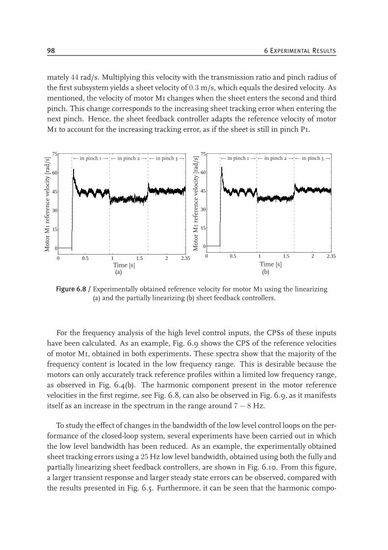
98 6 EXPERIMENTAL RESULTS
mately 44 rad/s. Multiplying this velocity with the transmission ratio and pinch radius ofthe first subsystem yields a sheet velocity of 0.3 m/s, which equals the desired velocity. Asmentioned, the velocity of motor M1 changes when the sheet enters the second and thirdpinch. This change corresponds to the increasing sheet tracking error when entering thenext pinch. Hence, the sheet feedback controller adapts the reference velocity of motorM1 to account for the increasing tracking error, as if the sheet is still in pinch P1.
0 0.5 1 1.5 2 2.35
0
15
30
45
60
75
Time [s]
Motor
M1reference
velocity[rad/s] ← in pinch 1→ ← in pinch 2→ ← in pinch 3→
(a)
0 0.5 1 1.5 2 2.35
0
15
30
45
60
75
Time [s]
Motor
M1reference
velocity[rad/s] ← in pinch 1→ ← in pinch 2→← in pinch 3→
(b)
Figure 6.8 / Experimentally obtained reference velocity for motor M1 using the linearizing(a) and the partially linearizing (b) sheet feedback controllers.
For the frequency analysis of the high level control inputs, the CPSs of these inputshave been calculated. As an example, Fig. 6.9 shows the CPS of the reference velocitiesof motor M1, obtained in both experiments. These spectra show that the majority of thefrequency content is located in the low frequency range. This is desirable because themotors can only accurately track reference profiles within a limited low frequency range,as observed in Fig. 6.4(b). The harmonic component present in the motor referencevelocities in the first regime, see Fig. 6.8, can also be observed in Fig. 6.9, as it manifestsitself as an increase in the spectrum in the range around 7 − 8 Hz.
To study the effect of changes in the bandwidth of the low level control loops on the per-formance of the closed-loop system, several experiments have been carried out in whichthe low level bandwidth has been reduced. As an example, the experimentally obtainedsheet tracking errors using a 25Hz low level bandwidth, obtained using both the fully andpartially linearizing sheet feedback controllers, are shown in Fig. 6.10. From this figure,a larger transient response and larger steady state errors can be observed, compared withthe results presented in Fig. 6.5. Furthermore, it can be seen that the harmonic compo-
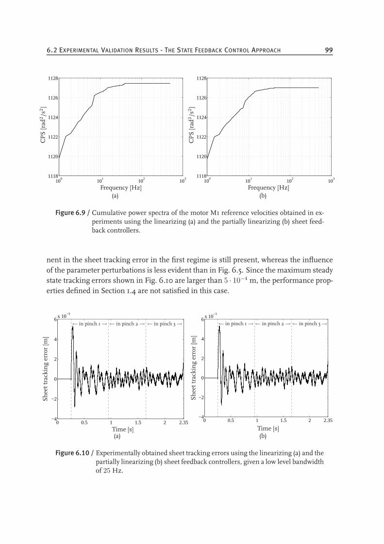
6.2 EXPERIMENTAL VALIDATION RESULTS - THE STATE FEEDBACK CONTROL APPROACH 99
100
101
102
103
1118
1120
1122
1124
1126
1128
Frequency [Hz]
CPS[rad
2/s
2]
(a)
100
101
102
103
1118
1120
1122
1124
1126
1128
Frequency [Hz]CPS[rad
2/s
2]
(b)
Figure 6.9 / Cumulative power spectra of the motor M1 reference velocities obtained in ex-periments using the linearizing (a) and the partially linearizing (b) sheet feed-back controllers.
nent in the sheet tracking error in the first regime is still present, whereas the influenceof the parameter perturbations is less evident than in Fig. 6.5. Since the maximum steadystate tracking errors shown in Fig. 6.10 are larger than 5 · 10−4 m, the performance prop-erties defined in Section 1.4 are not satisfied in this case.
0 0.5 1 1.5 2 2.35−4
−2
0
2
4
6x 10
−3
Time [s]
Sheettrackingerror[m
]
← in pinch 1→ ← in pinch 2→ ← in pinch 3→
(a)
0 0.5 1 1.5 2 2.35−4
−2
0
2
4
6x 10
−3
Time [s]
Sheettrackingerror[m
]
← in pinch 1→ ← in pinch 2→← in pinch 3→
(b)
Figure 6.10 / Experimentally obtained sheet tracking errors using the linearizing (a) and thepartially linearizing (b) sheet feedback controllers, given a low level bandwidthof 25 Hz.
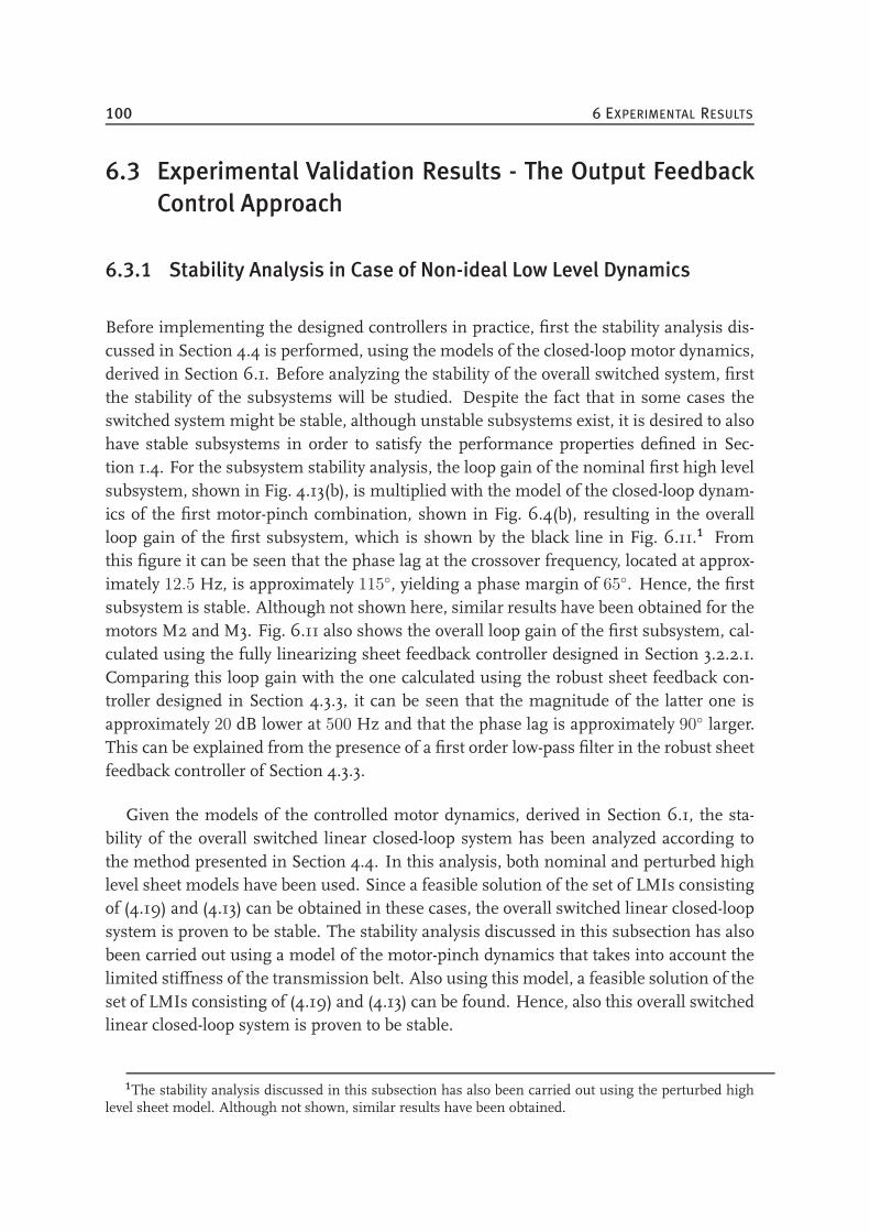
100 6 EXPERIMENTAL RESULTS
6.3 Experimental Validation Results - The Output Feedback
Control Approach
6.3.1 Stability Analysis in Case of Non-ideal Low Level Dynamics
Before implementing the designed controllers in practice, first the stability analysis dis-cussed in Section 4.4 is performed, using the models of the closed-loop motor dynamics,derived in Section 6.1. Before analyzing the stability of the overall switched system, firstthe stability of the subsystems will be studied. Despite the fact that in some cases theswitched system might be stable, although unstable subsystems exist, it is desired to alsohave stable subsystems in order to satisfy the performance properties defined in Sec-tion 1.4. For the subsystem stability analysis, the loop gain of the nominal first high levelsubsystem, shown in Fig. 4.13(b), is multiplied with the model of the closed-loop dynam-ics of the first motor-pinch combination, shown in Fig. 6.4(b), resulting in the overallloop gain of the first subsystem, which is shown by the black line in Fig. 6.11.1 Fromthis figure it can be seen that the phase lag at the crossover frequency, located at approx-imately 12.5 Hz, is approximately 115, yielding a phase margin of 65. Hence, the firstsubsystem is stable. Although not shown here, similar results have been obtained for themotors M2 and M3. Fig. 6.11 also shows the overall loop gain of the first subsystem, cal-culated using the fully linearizing sheet feedback controller designed in Section 3.2.2.1.Comparing this loop gain with the one calculated using the robust sheet feedback con-troller designed in Section 4.3.3, it can be seen that the magnitude of the latter one isapproximately 20 dB lower at 500 Hz and that the phase lag is approximately 90 larger.This can be explained from the presence of a first order low-pass filter in the robust sheetfeedback controller of Section 4.3.3.
Given the models of the controlled motor dynamics, derived in Section 6.1, the sta-bility of the overall switched linear closed-loop system has been analyzed according tothe method presented in Section 4.4. In this analysis, both nominal and perturbed highlevel sheet models have been used. Since a feasible solution of the set of LMIs consistingof (4.19) and (4.13) can be obtained in these cases, the overall switched linear closed-loopsystem is proven to be stable. The stability analysis discussed in this subsection has alsobeen carried out using a model of the motor-pinch dynamics that takes into account thelimited stiffness of the transmission belt. Also using this model, a feasible solution of theset of LMIs consisting of (4.19) and (4.13) can be found. Hence, also this overall switchedlinear closed-loop system is proven to be stable.
1The stability analysis discussed in this subsection has also been carried out using the perturbed highlevel sheet model. Although not shown, similar results have been obtained.
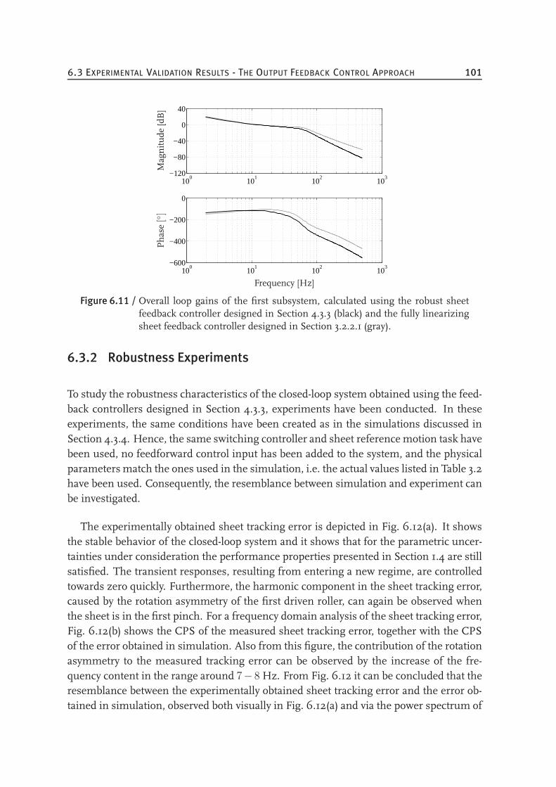
6.3 EXPERIMENTAL VALIDATION RESULTS - THE OUTPUT FEEDBACK CONTROL APPROACH 101
100
101
102
103
−120
−80
−40
0
40
100
101
102
103
−600
−400
−200
0
Magnitude
[dB]
Phase
[]
Frequency [Hz]
Figure 6.11 / Overall loop gains of the first subsystem, calculated using the robust sheetfeedback controller designed in Section 4.3.3 (black) and the fully linearizingsheet feedback controller designed in Section 3.2.2.1 (gray).
6.3.2 Robustness Experiments
To study the robustness characteristics of the closed-loop system obtained using the feed-back controllers designed in Section 4.3.3, experiments have been conducted. In theseexperiments, the same conditions have been created as in the simulations discussed inSection 4.3.4. Hence, the same switching controller and sheet referencemotion task havebeen used, no feedforward control input has been added to the system, and the physicalparametersmatch the ones used in the simulation, i.e. the actual values listed in Table 3.2have been used. Consequently, the resemblance between simulation and experiment canbe investigated.
The experimentally obtained sheet tracking error is depicted in Fig. 6.12(a). It showsthe stable behavior of the closed-loop system and it shows that for the parametric uncer-tainties under consideration the performance properties presented in Section 1.4 are stillsatisfied. The transient responses, resulting from entering a new regime, are controlledtowards zero quickly. Furthermore, the harmonic component in the sheet tracking error,caused by the rotation asymmetry of the first driven roller, can again be observed whenthe sheet is in the first pinch. For a frequency domain analysis of the sheet tracking error,Fig. 6.12(b) shows the CPS of the measured sheet tracking error, together with the CPSof the error obtained in simulation. Also from this figure, the contribution of the rotationasymmetry to the measured tracking error can be observed by the increase of the fre-quency content in the range around 7− 8 Hz. From Fig. 6.12 it can be concluded that theresemblance between the experimentally obtained sheet tracking error and the error ob-tained in simulation, observed both visually in Fig. 6.12(a) and via the power spectrum of
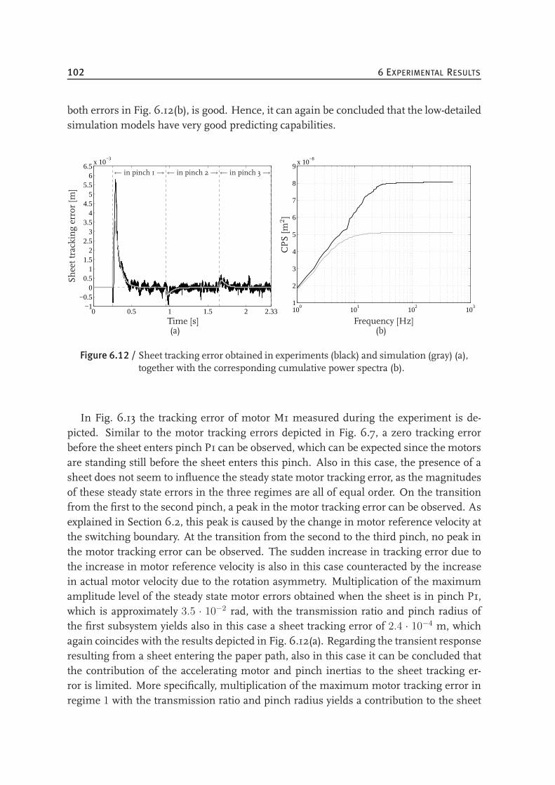
102 6 EXPERIMENTAL RESULTS
both errors in Fig. 6.12(b), is good. Hence, it can again be concluded that the low-detailedsimulation models have very good predicting capabilities.
0 0.5 1 1.5 2 2.33−1
−0.50
0.51
1.52
2.53
3.54
4.55
5.56
6.5x 10
−3
Time [s]
Sheettrackingerror[m
]
← in pinch 1→ ← in pinch 2→← in pinch 3→
(a)
100
101
102
103
1
2
3
4
5
6
7
8
9x 10
−8
Frequency [Hz]
CPS[m
2]
(b)
Figure 6.12 / Sheet tracking error obtained in experiments (black) and simulation (gray) (a),together with the corresponding cumulative power spectra (b).
In Fig. 6.13 the tracking error of motor M1 measured during the experiment is de-picted. Similar to the motor tracking errors depicted in Fig. 6.7, a zero tracking errorbefore the sheet enters pinch P1 can be observed, which can be expected since the motorsare standing still before the sheet enters this pinch. Also in this case, the presence of asheet does not seem to influence the steady state motor tracking error, as the magnitudesof these steady state errors in the three regimes are all of equal order. On the transitionfrom the first to the second pinch, a peak in the motor tracking error can be observed. Asexplained in Section 6.2, this peak is caused by the change in motor reference velocity atthe switching boundary. At the transition from the second to the third pinch, no peak inthe motor tracking error can be observed. The sudden increase in tracking error due tothe increase in motor reference velocity is also in this case counteracted by the increasein actual motor velocity due to the rotation asymmetry. Multiplication of the maximumamplitude level of the steady state motor errors obtained when the sheet is in pinch P1,which is approximately 3.5 · 10−2 rad, with the transmission ratio and pinch radius ofthe first subsystem yields also in this case a sheet tracking error of 2.4 · 10−4 m, whichagain coincides with the results depicted in Fig. 6.12(a). Regarding the transient responseresulting from a sheet entering the paper path, also in this case it can be concluded thatthe contribution of the accelerating motor and pinch inertias to the sheet tracking er-ror is limited. More specifically, multiplication of the maximum motor tracking error inregime 1 with the transmission ratio and pinch radius yields a contribution to the sheet
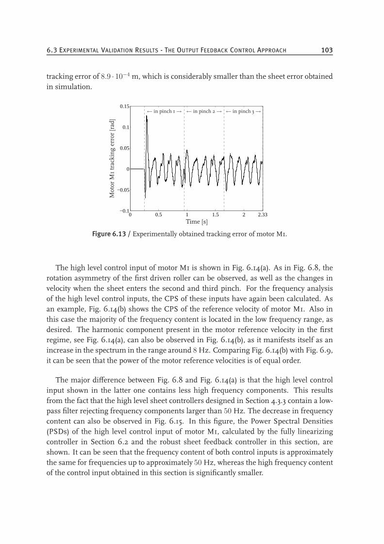
6.3 EXPERIMENTAL VALIDATION RESULTS - THE OUTPUT FEEDBACK CONTROL APPROACH 103
tracking error of 8.9 · 10−4 m, which is considerably smaller than the sheet error obtainedin simulation.
0 0.5 1 1.5 2 2.33−0.1
−0.05
0
0.05
0.1
0.15
Time [s]
Motor
M1trackingerror[rad]
← in pinch 1→ ← in pinch 2→ ← in pinch 3→
Figure 6.13 / Experimentally obtained tracking error of motor M1.
The high level control input of motor M1 is shown in Fig. 6.14(a). As in Fig. 6.8, therotation asymmetry of the first driven roller can be observed, as well as the changes invelocity when the sheet enters the second and third pinch. For the frequency analysisof the high level control inputs, the CPS of these inputs have again been calculated. Asan example, Fig. 6.14(b) shows the CPS of the reference velocity of motor M1. Also inthis case the majority of the frequency content is located in the low frequency range, asdesired. The harmonic component present in the motor reference velocity in the firstregime, see Fig. 6.14(a), can also be observed in Fig. 6.14(b), as it manifests itself as anincrease in the spectrum in the range around 8 Hz. Comparing Fig. 6.14(b) with Fig. 6.9,it can be seen that the power of the motor reference velocities is of equal order.
The major difference between Fig. 6.8 and Fig. 6.14(a) is that the high level controlinput shown in the latter one contains less high frequency components. This resultsfrom the fact that the high level sheet controllers designed in Section 4.3.3 contain a low-pass filter rejecting frequency components larger than 50 Hz. The decrease in frequencycontent can also be observed in Fig. 6.15. In this figure, the Power Spectral Densities(PSDs) of the high level control input of motor M1, calculated by the fully linearizingcontroller in Section 6.2 and the robust sheet feedback controller in this section, areshown. It can be seen that the frequency content of both control inputs is approximatelythe same for frequencies up to approximately 50 Hz, whereas the high frequency contentof the control input obtained in this section is significantly smaller.
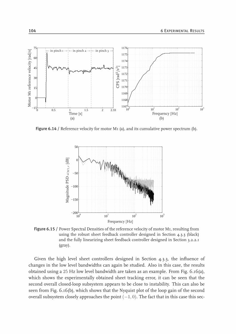
104 6 EXPERIMENTAL RESULTS
0 0.5 1 1.5 2 2.33−15
0
15
30
45
60
75
Time [s]
Motor
M1reference
velocity[rad/s] ← in pinch 1→ ← in pinch 2→← in pinch 3→
(a)
100
101
102
103
1167
1168
1169
1170
1171
1172
1173
1174
1175
1176
Frequency [Hz]CPS[rad
2/s
2]
(b)
Figure 6.14 / Reference velocity for motor M1 (a), and its cumulative power spectrum (b).
100
101
102
103
−200
−150
−100
−50
0
50
Frequency [Hz]
Magnitude
PSD
ωM
1,r[dB]
Figure 6.15 / Power Spectral Densities of the reference velocity of motor M1, resulting fromusing the robust sheet feedback controller designed in Section 4.3.3 (black)and the fully linearizing sheet feedback controller designed in Section 3.2.2.1(gray).
Given the high level sheet controllers designed in Section 4.3.3, the influence ofchanges in the low level bandwidths can again be studied. Also in this case, the resultsobtained using a 25 Hz low level bandwidth are taken as an example. From Fig. 6.16(a),which shows the experimentally obtained sheet tracking error, it can be seen that thesecond overall closed-loop subsystem appears to be close to instability. This can also beseen from Fig. 6.16(b), which shows that the Nyquist plot of the loop gain of the secondoverall subsystem closely approaches the point (−1, 0). The fact that in this case this sec-
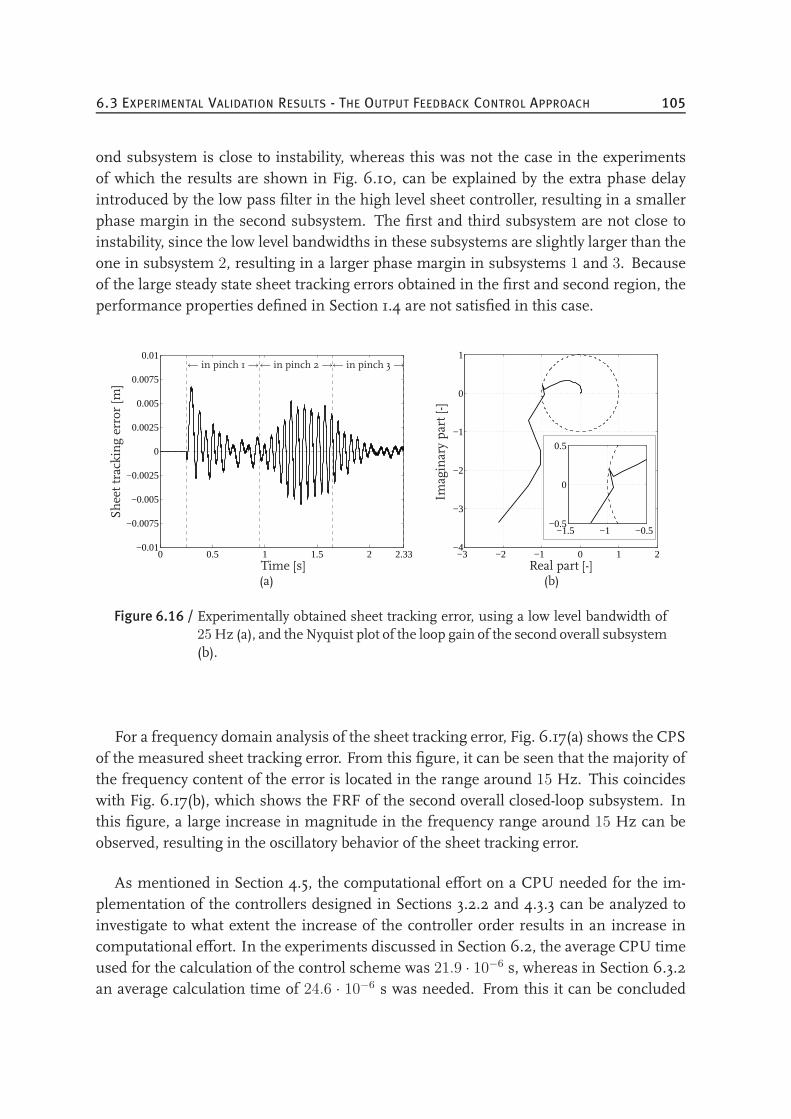
6.3 EXPERIMENTAL VALIDATION RESULTS - THE OUTPUT FEEDBACK CONTROL APPROACH 105
ond subsystem is close to instability, whereas this was not the case in the experimentsof which the results are shown in Fig. 6.10, can be explained by the extra phase delayintroduced by the low pass filter in the high level sheet controller, resulting in a smallerphase margin in the second subsystem. The first and third subsystem are not close toinstability, since the low level bandwidths in these subsystems are slightly larger than theone in subsystem 2, resulting in a larger phase margin in subsystems 1 and 3. Becauseof the large steady state sheet tracking errors obtained in the first and second region, theperformance properties defined in Section 1.4 are not satisfied in this case.
0 0.5 1 1.5 2 2.33−0.01
−0.0075
−0.005
−0.0025
0
0.0025
0.005
0.0075
0.01
Time [s]
Sheettrackingerror[m
]
← in pinch 1→← in pinch 2→← in pinch 3→
(a)
−3 −2 −1 0 1 2−4
−3
−2
−1
0
1
−1.5 −1 −0.5−0.5
0
0.5
Real part [-]
Imaginarypart[-]
(b)
Figure 6.16 / Experimentally obtained sheet tracking error, using a low level bandwidth of25Hz (a), and the Nyquist plot of the loop gain of the second overall subsystem(b).
For a frequency domain analysis of the sheet tracking error, Fig. 6.17(a) shows the CPSof the measured sheet tracking error. From this figure, it can be seen that the majority ofthe frequency content of the error is located in the range around 15 Hz. This coincideswith Fig. 6.17(b), which shows the FRF of the second overall closed-loop subsystem. Inthis figure, a large increase in magnitude in the frequency range around 15 Hz can beobserved, resulting in the oscillatory behavior of the sheet tracking error.
As mentioned in Section 4.5, the computational effort on a CPU needed for the im-plementation of the controllers designed in Sections 3.2.2 and 4.3.3 can be analyzed toinvestigate to what extent the increase of the controller order results in an increase incomputational effort. In the experiments discussed in Section 6.2, the average CPU timeused for the calculation of the control scheme was 21.9 · 10−6 s, whereas in Section 6.3.2an average calculation time of 24.6 · 10−6 s was needed. From this it can be concluded
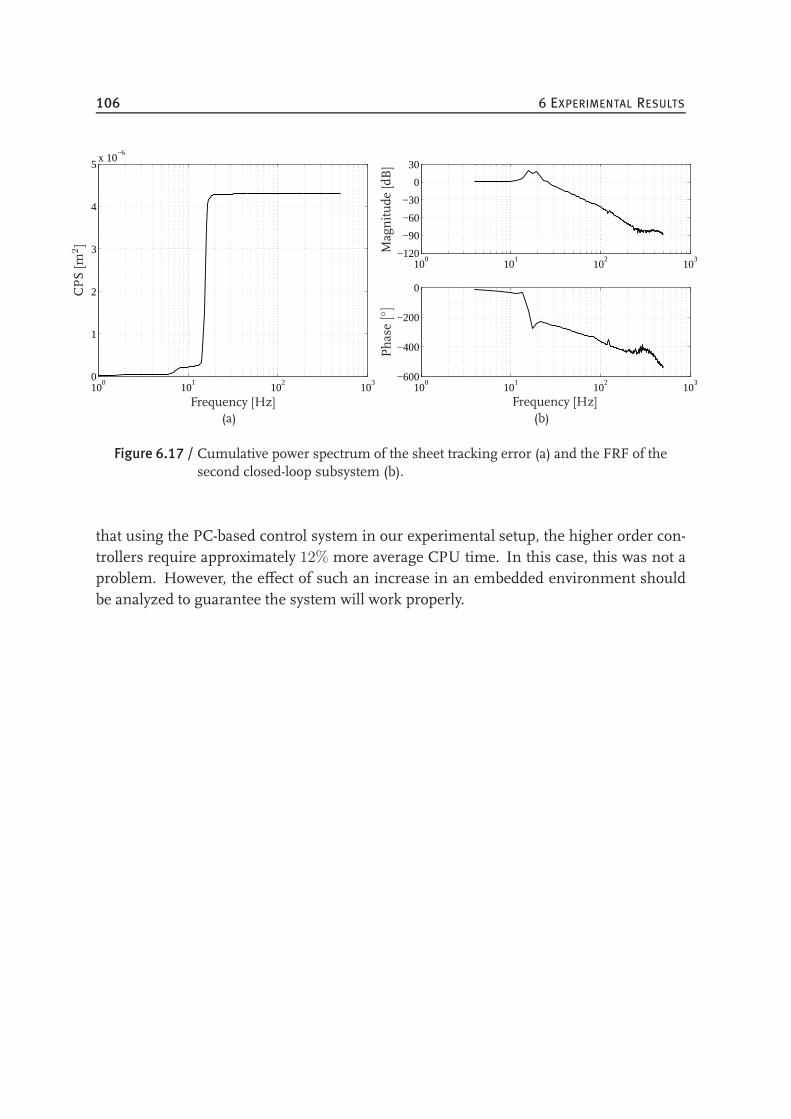
106 6 EXPERIMENTAL RESULTS
100
101
102
103
0
1
2
3
4
5x 10
−6
Frequency [Hz]
CPS[m
2]
(a)
100
101
102
103
−120
−90
−60
−30
0
30
100
101
102
103
−600
−400
−200
0
Magnitude
[dB]
Phase
[]
Frequency [Hz](b)
Figure 6.17 / Cumulative power spectrum of the sheet tracking error (a) and the FRF of thesecond closed-loop subsystem (b).
that using the PC-based control system in our experimental setup, the higher order con-trollers require approximately 12% more average CPU time. In this case, this was not aproblem. However, the effect of such an increase in an embedded environment shouldbe analyzed to guarantee the system will work properly.

CHAPTER SEVEN
Extensions of Sheet Feedback Control toReal Printer Paper Paths
7.1 Challenges in Industrial Paper Paths . . . . . . . . . . . . . . . . . . . . 107
7.2 Duplex Loop Modeling and Control . . . . . . . . . . . . . . . . . . . . . 108
7.3 Sheet Transport via Multiple Pinches . . . . . . . . . . . . . . . . . . . . 113
7.4 Coupling Pinches into Sections . . . . . . . . . . . . . . . . . . . . . . . 128
7.5 Evaluation . . . . . . . . . . . . . . . . . . . . . . . . . . . . . . . . . . . 130
7.1 Challenges in Industrial Paper Paths
In Chapter 2, a basic paper path was chosen as a case-study for sheet feedback controldesign. So far, some of the challenging aspects of real printer paper paths have delib-erately been left out of consideration to reveal the essence of the control problem. Thethree main differences between the basic paper path and real paper path layouts, as theone shown in Fig.1.3, are
1. the absence of a duplex loop for backside printing,
2. the distances between the pinches being equal to the sheet length,
3. and the actuation of each pinch by a separate motor.
To bridge the gap between the design of sheet feedback controllers for the basic paperpath and a real paper path, this chapter will describe sheet feedback control design for
107
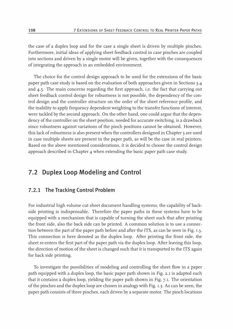
108 7 EXTENSIONS OF SHEET FEEDBACK CONTROL TO REAL PRINTER PAPER PATHS
the case of a duplex loop and for the case a single sheet is driven by multiple pinches.Furthermore, initial ideas of applying sheet feedback control in case pinches are coupledinto sections and driven by a single motor will be given, together with the consequencesof integrating the approach in an embedded environment.
The choice for the control design approach to be used for the extensions of the basicpaper path case study is based on the evaluation of both approaches given in Sections 3.4and 4.5. The main concerns regarding the first approach, i.e. the fact that carrying outsheet feedback control design for robustness is not possible, the dependency of the con-trol design and the controller structure on the order of the sheet reference profile, andthe inability to apply frequency dependent weighting to the transfer functions of interest,were tackled by the second approach. On the other hand, one could argue that the depen-dency of the controller on the sheet position, needed for accurate switching, is a drawbacksince robustness against variations of the pinch positions cannot be obtained. However,this lack of robustness is also present when the controllers designed in Chapter 3 are usedin case multiple sheets are present in the paper path, as will be the case in real printers.Based on the above mentioned considerations, it is decided to choose the control designapproach described in Chapter 4 when extending the basic paper path case study.
7.2 Duplex Loop Modeling and Control
7.2.1 The Tracking Control Problem
For industrial high volume cut sheet document handling systems, the capability of back-side printing is indispensable. Therefore the paper paths in these systems have to beequipped with a mechanism that is capable of turning the sheet such that after printingthe front side, also the back side can be printed. A common solution is to use a connec-tion between the part of the paper path before and after the ITS, as can be seen in Fig. 1.3.This connection is here denoted as the duplex loop. After printing the front side, thesheet re-enters the first part of the paper path via the duplex loop. After leaving this loop,the direction of motion of the sheet is changed such that it is transported to the ITS againfor back side printing.
To investigate the possibilities of modeling and controlling the sheet flow in a paperpath equipped with a duplex loop, the basic paper path shown in Fig. 2.1 is adapted suchthat it contains a duplex loop, yielding the paper path shown in Fig. 7.1. The orientationof the pinches and the duplex loop are chosen in analogy with Fig. 1.3. As can be seen, thepaper path consists of three pinches, each driven by a separatemotor. The pinch locations
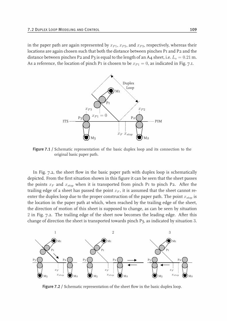
7.2 DUPLEX LOOP MODELING AND CONTROL 109
in the paper path are again represented by xP1, xP2, and xP3, respectively, whereas theirlocations are again chosen such that both the distance between pinches P1 and P2 and thedistance between pinches P2 and P3 is equal to the length of an A4 sheet, i.e.Ls = 0.21m.As a reference, the location of pinch P1 is chosen to be xP1 = 0, as indicated in Fig. 7.1.
M1
M2M3
P1
P2P3xP1 = 0
xP2xP3
xF xstop
PIMITS
DuplexLoop
Figure 7.1 / Schematic representation of the basic duplex loop and its connection to theoriginal basic paper path.
In Fig. 7.2, the sheet flow in the basic paper path with duplex loop is schematicallydepicted. From the first situation shown in this figure it can be seen that the sheet passesthe points xF and xstop when it is transported from pinch P1 to pinch P2. After thetrailing edge of a sheet has passed the point xF , it is assumed that the sheet cannot re-enter the duplex loop due to the proper construction of the paper path. The point xstop isthe location in the paper path at which, when reached by the trailing edge of the sheet,the direction of motion of this sheet is supposed to change, as can be seen by situation2 in Fig. 7.2. The trailing edge of the sheet now becomes the leading edge. After thischange of direction the sheet is transported towards pinch P3, as indicated by situation 3.
M1M1M1
M2M2M2 M3M3M3
P1P1P1
P2P2P2 P3P3P3
xFxFxF
xstopxstopxstop
1 2 3
Figure 7.2 / Schematic representation of the sheet flow in the basic duplex loop.
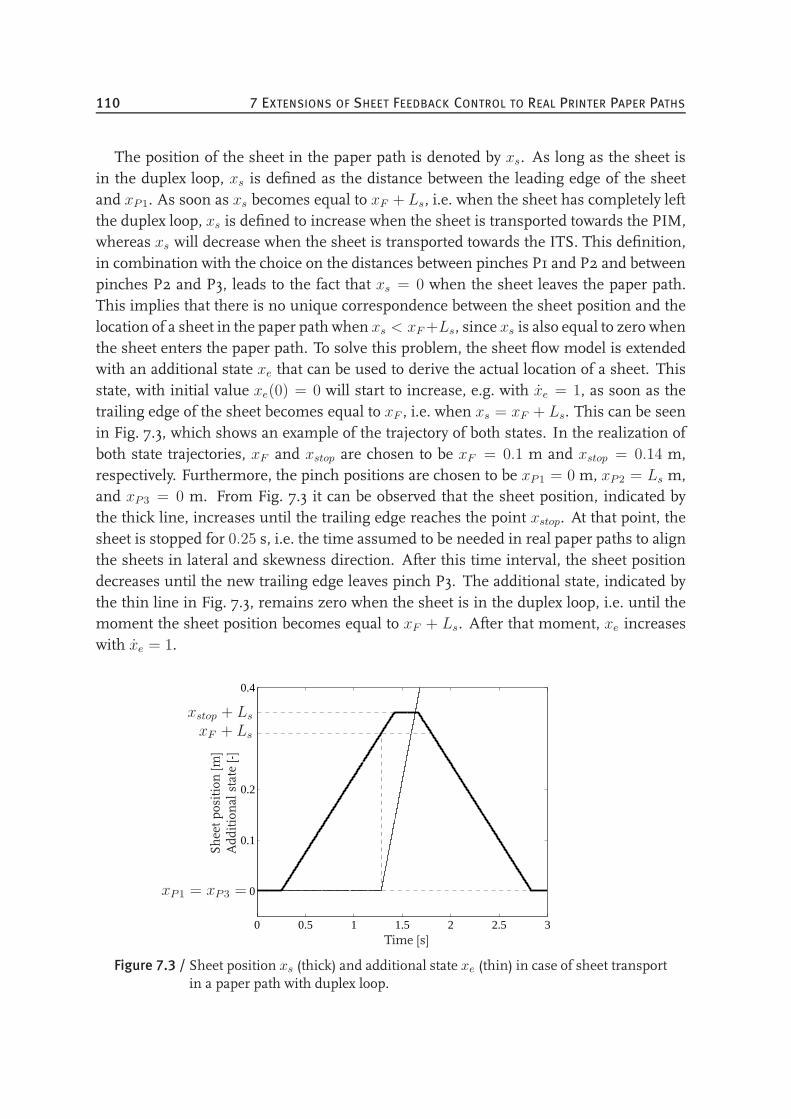
110 7 EXTENSIONS OF SHEET FEEDBACK CONTROL TO REAL PRINTER PAPER PATHS
The position of the sheet in the paper path is denoted by xs. As long as the sheet isin the duplex loop, xs is defined as the distance between the leading edge of the sheetand xP1. As soon as xs becomes equal to xF + Ls, i.e. when the sheet has completely leftthe duplex loop, xs is defined to increase when the sheet is transported towards the PIM,whereas xs will decrease when the sheet is transported towards the ITS. This definition,in combination with the choice on the distances between pinches P1 and P2 and betweenpinches P2 and P3, leads to the fact that xs = 0 when the sheet leaves the paper path.This implies that there is no unique correspondence between the sheet position and thelocation of a sheet in the paper path when xs < xF+Ls, since xs is also equal to zero whenthe sheet enters the paper path. To solve this problem, the sheet flow model is extendedwith an additional state xe that can be used to derive the actual location of a sheet. Thisstate, with initial value xe(0) = 0 will start to increase, e.g. with xe = 1, as soon as thetrailing edge of the sheet becomes equal to xF , i.e. when xs = xF + Ls. This can be seenin Fig. 7.3, which shows an example of the trajectory of both states. In the realization ofboth state trajectories, xF and xstop are chosen to be xF = 0.1 m and xstop = 0.14 m,respectively. Furthermore, the pinch positions are chosen to be xP1 = 0 m, xP2 = Ls m,and xP3 = 0 m. From Fig. 7.3 it can be observed that the sheet position, indicated bythe thick line, increases until the trailing edge reaches the point xstop. At that point, thesheet is stopped for 0.25 s, i.e. the time assumed to be needed in real paper paths to alignthe sheets in lateral and skewness direction. After this time interval, the sheet positiondecreases until the new trailing edge leaves pinch P3. The additional state, indicated bythe thin line in Fig. 7.3, remains zero when the sheet is in the duplex loop, i.e. until themoment the sheet position becomes equal to xF + Ls. After that moment, xe increaseswith xe = 1.
0 0.5 1 1.5 2 2.5 3
0
0.1
0.2
0.4
Time [s]
Sheetp
osition[m
]Add
itionalstate[-]
xF + Ls
xstop + Ls
xP1 = xP3 =
Figure 7.3 / Sheet position xs (thick) and additional state xe (thin) in case of sheet transportin a paper path with duplex loop.
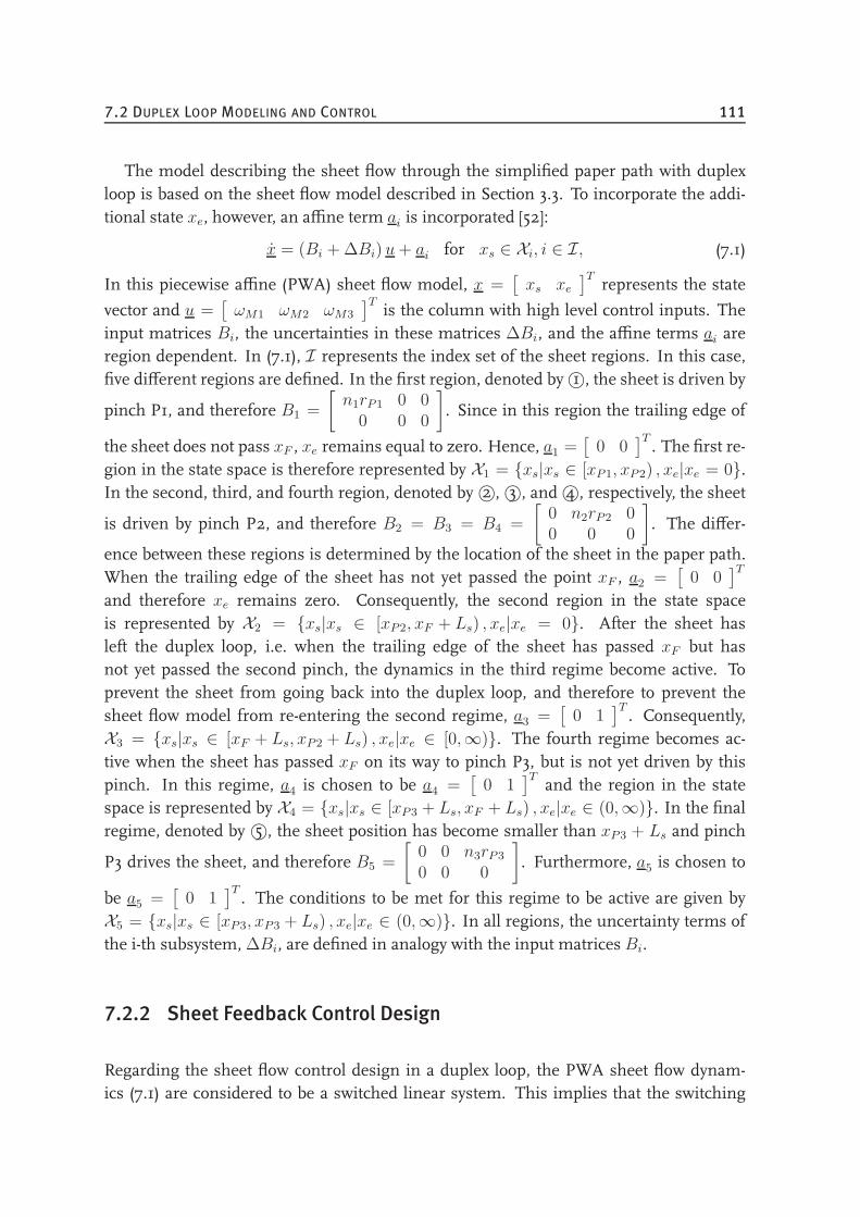
7.2 DUPLEX LOOP MODELING AND CONTROL 111
The model describing the sheet flow through the simplified paper path with duplexloop is based on the sheet flow model described in Section 3.3. To incorporate the addi-tional state xe, however, an affine term ai is incorporated [52]:
x = (Bi + ∆Bi) u+ ai for xs ∈ Xi, i ∈ I, (7.1)
In this piecewise affine (PWA) sheet flow model, x =[xs xe
]Trepresents the state
vector and u =[ωM1 ωM2 ωM3
]Tis the column with high level control inputs. The
input matrices Bi, the uncertainties in these matrices ∆Bi, and the affine terms ai areregion dependent. In (7.1), I represents the index set of the sheet regions. In this case,five different regions are defined. In the first region, denoted by 1©, the sheet is driven by
pinch P1, and therefore B1 =
[n1rP1 0 0
0 0 0
]. Since in this region the trailing edge of
the sheet does not pass xF , xe remains equal to zero. Hence, a1 =[
0 0]T. The first re-
gion in the state space is therefore represented by X1 = xs|xs ∈ [xP1, xP2) , xe|xe = 0.In the second, third, and fourth region, denoted by 2©, 3©, and 4©, respectively, the sheet
is driven by pinch P2, and therefore B2 = B3 = B4 =
[0 n2rP2 00 0 0
]. The differ-
ence between these regions is determined by the location of the sheet in the paper path.When the trailing edge of the sheet has not yet passed the point xF , a2 =
[0 0
]T
and therefore xe remains zero. Consequently, the second region in the state spaceis represented by X2 = xs|xs ∈ [xP2, xF + Ls) , xe|xe = 0. After the sheet hasleft the duplex loop, i.e. when the trailing edge of the sheet has passed xF but hasnot yet passed the second pinch, the dynamics in the third regime become active. Toprevent the sheet from going back into the duplex loop, and therefore to prevent thesheet flow model from re-entering the second regime, a3 =
[0 1
]T. Consequently,
X3 = xs|xs ∈ [xF + Ls, xP2 + Ls) , xe|xe ∈ [0,∞). The fourth regime becomes ac-tive when the sheet has passed xF on its way to pinch P3, but is not yet driven by thispinch. In this regime, a4 is chosen to be a4 =
[0 1
]Tand the region in the state
space is represented by X4 = xs|xs ∈ [xP3 + Ls, xF + Ls) , xe|xe ∈ (0,∞). In the finalregime, denoted by 5©, the sheet position has become smaller than xP3 + Ls and pinch
P3 drives the sheet, and therefore B5 =
[0 0 n3rP3
0 0 0
]. Furthermore, a5 is chosen to
be a5 =[
0 1]T. The conditions to be met for this regime to be active are given by
X5 = xs|xs ∈ [xP3, xP3 + Ls) , xe|xe ∈ (0,∞). In all regions, the uncertainty terms ofthe i-th subsystem, ∆Bi, are defined in analogy with the input matrices Bi.
7.2.2 Sheet Feedback Control Design
Regarding the sheet flow control design in a duplex loop, the PWA sheet flow dynam-ics (7.1) are considered to be a switched linear system. This implies that the switching
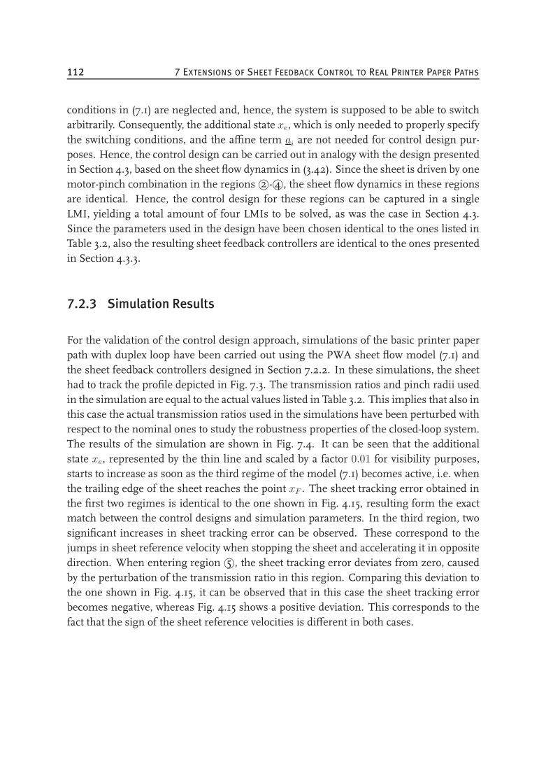
112 7 EXTENSIONS OF SHEET FEEDBACK CONTROL TO REAL PRINTER PAPER PATHS
conditions in (7.1) are neglected and, hence, the system is supposed to be able to switcharbitrarily. Consequently, the additional state xe, which is only needed to properly specifythe switching conditions, and the affine term ai are not needed for control design pur-poses. Hence, the control design can be carried out in analogy with the design presentedin Section 4.3, based on the sheet flow dynamics in (3.42). Since the sheet is driven by onemotor-pinch combination in the regions 2©- 4©, the sheet flow dynamics in these regionsare identical. Hence, the control design for these regions can be captured in a singleLMI, yielding a total amount of four LMIs to be solved, as was the case in Section 4.3.Since the parameters used in the design have been chosen identical to the ones listed inTable 3.2, also the resulting sheet feedback controllers are identical to the ones presentedin Section 4.3.3.
7.2.3 Simulation Results
For the validation of the control design approach, simulations of the basic printer paperpath with duplex loop have been carried out using the PWA sheet flow model (7.1) andthe sheet feedback controllers designed in Section 7.2.2. In these simulations, the sheethad to track the profile depicted in Fig. 7.3. The transmission ratios and pinch radii usedin the simulation are equal to the actual values listed in Table 3.2. This implies that also inthis case the actual transmission ratios used in the simulations have been perturbed withrespect to the nominal ones to study the robustness properties of the closed-loop system.The results of the simulation are shown in Fig. 7.4. It can be seen that the additionalstate xe, represented by the thin line and scaled by a factor 0.01 for visibility purposes,starts to increase as soon as the third regime of the model (7.1) becomes active, i.e. whenthe trailing edge of the sheet reaches the point xF . The sheet tracking error obtained inthe first two regimes is identical to the one shown in Fig. 4.15, resulting form the exactmatch between the control designs and simulation parameters. In the third region, twosignificant increases in sheet tracking error can be observed. These correspond to thejumps in sheet reference velocity when stopping the sheet and accelerating it in oppositedirection. When entering region 5©, the sheet tracking error deviates from zero, causedby the perturbation of the transmission ratio in this region. Comparing this deviation tothe one shown in Fig. 4.15, it can be observed that in this case the sheet tracking errorbecomes negative, whereas Fig. 4.15 shows a positive deviation. This corresponds to thefact that the sign of the sheet reference velocities is different in both cases.
7.3 SHEET TRANSPORT VIA MULTIPLE PINCHES 113
0 0.5 1 1.5 2 2.5 3−4
−3
−2
−1
0
1
2
3
4
5x 10
−3
Time [s]
Sheettrackingerror[m
]Add
itionalstate[-]
←− 1© −→← 2©→← 3© →← 4©→←− 5© −→
Figure 7.4 / Sheet tracking error (thick) and additional state (thin) obtained in simulationin case of sheet transport in a duplex loop.
7.3 Sheet Transport via Multiple Pinches
7.3.1 The Tracking Control Problem
Besides two-sided printing, another important requirement for document handling sys-tems is the capability of transporting sheets with different dimensions. This implies thatone of the assumptions made in Section 2.1, i.e. the distances between the pinches beingequal to the sheet length, does not hold anymore. More specifically, these distances mustalways be smaller than or equal to the length of the smallest sheet to be transported.Hence, the situation in which multiple pinches are driving a single sheet will occur inreal printers for the larger sheet sizes, resulting in a coupling of the dynamics of differentmotor-pinch combinations via the sheet.
Before going into further detail on the control problem at hand, we will first presentthe case-study adopted in this section, in order to facilitate the reasoning about the controlproblem. In this case study, the paper path depicted in Fig. 7.5 is considered. In this paperpath an A3-format sheet, the length of which is 0.42 m, is transported by two pinches,each connected to a separate motor. The distance between these pinches is chosen to be0.21 m, which corresponds to the size of an A4-format sheet. The sheet position xs isagain defined as the position of the leading edge of the sheet in the paper path.
From Fig. 7.5, it can be derived that when the sheet is in both pinches, two additionalphenomena can occur in contrast with the case-study presented in Section 2.1. First of
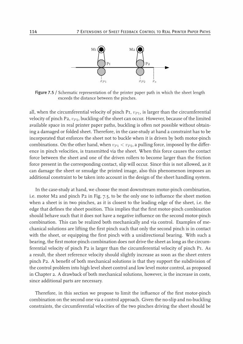
114 7 EXTENSIONS OF SHEET FEEDBACK CONTROL TO REAL PRINTER PAPER PATHS
M1 M2
P1 P2
xP1 xP2 xs
Figure 7.5 / Schematic representation of the printer paper path in which the sheet lengthexceeds the distance between the pinches.
all, when the circumferential velocity of pinch P1, vP1, is larger than the circumferentialvelocity of pinch P2, vP2, buckling of the sheet can occur. However, because of the limitedavailable space in real printer paper paths, buckling is often not possible without obtain-ing a damaged or folded sheet. Therefore, in the case-study at hand a constraint has to beincorporated that enforces the sheet not to buckle when it is driven by both motor-pinchcombinations. On the other hand, when vP1 < vP2, a pulling force, imposed by the differ-ence in pinch velocities, is transmitted via the sheet. When this force causes the contactforce between the sheet and one of the driven rollers to become larger than the frictionforce present in the corresponding contact, slip will occur. Since this is not allowed, as itcan damage the sheet or smudge the printed image, also this phenomenon imposes anadditional constraint to be taken into account in the design of the sheet handling system.
In the case-study at hand, we choose the most downstreammotor-pinch combination,i.e. motor M2 and pinch P2 in Fig. 7.5, to be the only one to influence the sheet motionwhen a sheet is in two pinches, as it is closest to the leading edge of the sheet, i.e. theedge that defines the sheet position. This implies that the first motor-pinch combinationshould behave such that it does not have a negative influence on the second motor-pinchcombination. This can be realized both mechanically and via control. Examples of me-chanical solutions are lifting the first pinch such that only the second pinch is in contactwith the sheet, or equipping the first pinch with a unidirectional bearing. With such abearing, the first motor-pinch combination does not drive the sheet as long as the circum-ferential velocity of pinch P2 is larger than the circumferential velocity of pinch P1. Asa result, the sheet reference velocity should slightly increase as soon as the sheet enterspinch P2. A benefit of both mechanical solutions is that they support the subdivision ofthe control problem into high level sheet control and low level motor control, as proposedin Chapter 2. A drawback of both mechanical solutions, however, is the increase in costs,since additional parts are necessary.
Therefore, in this section we propose to limit the influence of the first motor-pinchcombination on the second one via a control approach. Given the no-slip and no-bucklingconstraints, the circumferential velocities of the two pinches driving the sheet should be
7.3 SHEET TRANSPORT VIA MULTIPLE PINCHES 115
equal. To realize this goal, funnel-shaped velocity bounds, as proposed in [12, 13, 46],could be used in combination with the sheet feedback controllers designed in Sec-tion 4.3.3. However, in case parametric uncertainties are present in the paper path, perfectsynchronization of the circumferential pinch velocities cannot be guaranteed. Hence, inthis section the goal is to apply the systematic, model-based methodology for sheet feed-back control design presented in Chapters 2 and 4, taking into account the two additionalconstraints. To realize this goal, two questions have to be answered first:
1. Can the control problem still be decoupled into low level motor control and highlevel sheet control?
2. Can we still ensure the difference in high level and low level bandwidth and a goodlow level tracking behavior, such that the controlled motor dynamics can be as-sumed to be ideal when designing the sheet control loop?
Regarding the first question, we know that if the pulling force in the sheet is limited, thecontact forces present between the driven rollers and the sheet will be limited as well, andno slip will occur between the sheet and the pinches. Hence, similar to Section 2.3, a de-coupling into low level motor control and high level sheet control is possible. Limitationof the pulling force in the sheet can be realized by adapting the low level control strat-egy of motor M1 at the moment the sheet is driven by both pinches. In this adaptation,however, care has to be taken to ensure that buckling of the sheet does not occur either.The adaptation of the control strategy is necessary, since applying the original high gainPID feedback controller to both motors in case the sheet is in two pinches and in case thepaper path parameters are perturbed will result in slip between the sheet and one of thepinches. This can be explained by the fact that in this case both controlled motors will tryto closely track their reference velocities. However, due to the uncertainties in the paperpath parameters, the values of the motor reference velocities can be such that the corre-sponding circumferential pinch velocities are not equal. Therefore, it is not possible forboth motors to accurately track their reference velocities without slip between the sheetand both pinches. Hence, the control action for one or both motors, and therefore thecontact force between the sheet and the driven roller and the pulling force transmitted viathe sheet, will increase until slip between the sheet and one of the pinches will occur.
The answer to the second question follows from the choice that when the sheet is intwo pinches, the downstreammotor-pinch combination determines the sheet motion andthe upstreammotor-pinch combination follows this motion without strongly influencingthe behavior of the downstream motor and pinch. Hence, if the downstream motor con-trol loop, i.e. the control loop for motor M2, has a good tracking behavior and is designedto have a higher bandwidth than the sheet control loop, satisfying the rules of thumb usedin hierarchical control design [75], the controlled motors can be assumed to be ideal.
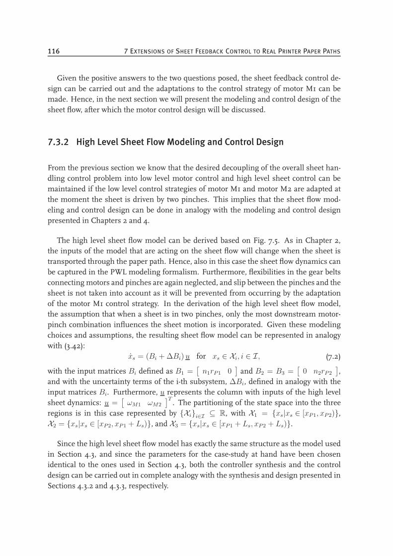
116 7 EXTENSIONS OF SHEET FEEDBACK CONTROL TO REAL PRINTER PAPER PATHS
Given the positive answers to the two questions posed, the sheet feedback control de-sign can be carried out and the adaptations to the control strategy of motor M1 can bemade. Hence, in the next section we will present the modeling and control design of thesheet flow, after which the motor control design will be discussed.
7.3.2 High Level Sheet Flow Modeling and Control Design
From the previous section we know that the desired decoupling of the overall sheet han-dling control problem into low level motor control and high level sheet control can bemaintained if the low level control strategies of motor M1 and motor M2 are adapted atthe moment the sheet is driven by two pinches. This implies that the sheet flow mod-eling and control design can be done in analogy with the modeling and control designpresented in Chapters 2 and 4.
The high level sheet flow model can be derived based on Fig. 7.5. As in Chapter 2,the inputs of the model that are acting on the sheet flow will change when the sheet istransported through the paper path. Hence, also in this case the sheet flow dynamics canbe captured in the PWL modeling formalism. Furthermore, flexibilities in the gear beltsconnecting motors and pinches are again neglected, and slip between the pinches and thesheet is not taken into account as it will be prevented from occurring by the adaptationof the motor M1 control strategy. In the derivation of the high level sheet flow model,the assumption that when a sheet is in two pinches, only the most downstream motor-pinch combination influences the sheet motion is incorporated. Given these modelingchoices and assumptions, the resulting sheet flow model can be represented in analogywith (3.42):
xs = (Bi + ∆Bi) u for xs ∈ Xi, i ∈ I, (7.2)
with the input matrices Bi defined as B1 =[n1rP1 0
]and B2 = B3 =
[0 n2rP2
],
and with the uncertainty terms of the i-th subsystem, ∆Bi, defined in analogy with theinput matrices Bi. Furthermore, u represents the column with inputs of the high levelsheet dynamics: u =
[ωM1 ωM2
]T. The partitioning of the state space into the three
regions is in this case represented by Xii∈I ⊆ R, with X1 = xs|xs ∈ [xP1, xP2),X2 = xs|xs ∈ [xP2, xP1 + Ls), and X3 = xs|xs ∈ [xP1 + Ls, xP2 + Ls).
Since the high level sheet flow model has exactly the same structure as the model usedin Section 4.3, and since the parameters for the case-study at hand have been chosenidentical to the ones used in Section 4.3, both the controller synthesis and the controldesign can be carried out in complete analogy with the synthesis and design presented inSections 4.3.2 and 4.3.3, respectively.
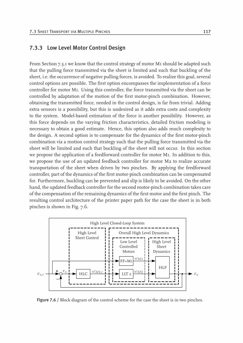
7.3 SHEET TRANSPORT VIA MULTIPLE PINCHES 117
7.3.3 Low Level Motor Control Design
From Section 7.3.1 we know that the control strategy of motor M1 should be adapted suchthat the pulling force transmitted via the sheet is limited and such that buckling of thesheet, i.e. the occurrence of negative pulling forces, is avoided. To realize this goal, severalcontrol options are possible. The first option encompasses the implementation of a forcecontroller for motor M1. Using this controller, the force transmitted via the sheet can becontrolled by adaptation of the motion of the first motor-pinch combination. However,obtaining the transmitted force, needed in the control design, is far from trivial. Addingextra sensors is a possibility, but this is undesired as it adds extra costs and complexityto the system. Model-based estimation of the force is another possibility. However, asthis force depends on the varying friction characteristics, detailed friction modeling isnecessary to obtain a good estimate. Hence, this option also adds much complexity tothe design. A second option is to compensate for the dynamics of the first motor-pinchcombination via a motion control strategy such that the pulling force transmitted via thesheet will be limited and such that buckling of the sheet will not occur. In this sectionwe propose the application of a feedforward controller for motor M1. In addition to this,we propose the use of an updated feedback controller for motor M2 to realize accuratetransportation of the sheet when driven by two pinches. By applying the feedforwardcontroller, part of the dynamics of the first motor-pinch combination can be compensatedfor. Furthermore, buckling can be prevented and slip is likely to be avoided. On the otherhand, the updated feedback controller for the secondmotor-pinch combination takes careof the compensation of the remaining dynamics of the first motor and the first pinch. Theresulting control architecture of the printer paper path for the case the sheet is in bothpinches is shown in Fig. 7.6.
+_
HLC
FF+M1
LLT 2
HLPωM2,r
Low LevelControlledMotors
High LevelSheet
Dynamics
High LevelSheet Control
Overall High Level Dynamics
High Level Closed-Loop System
xs,r xs
ωM1
ωM2es
Figure 7.6 / Block diagram of the control scheme for the case the sheet is in two pinches.
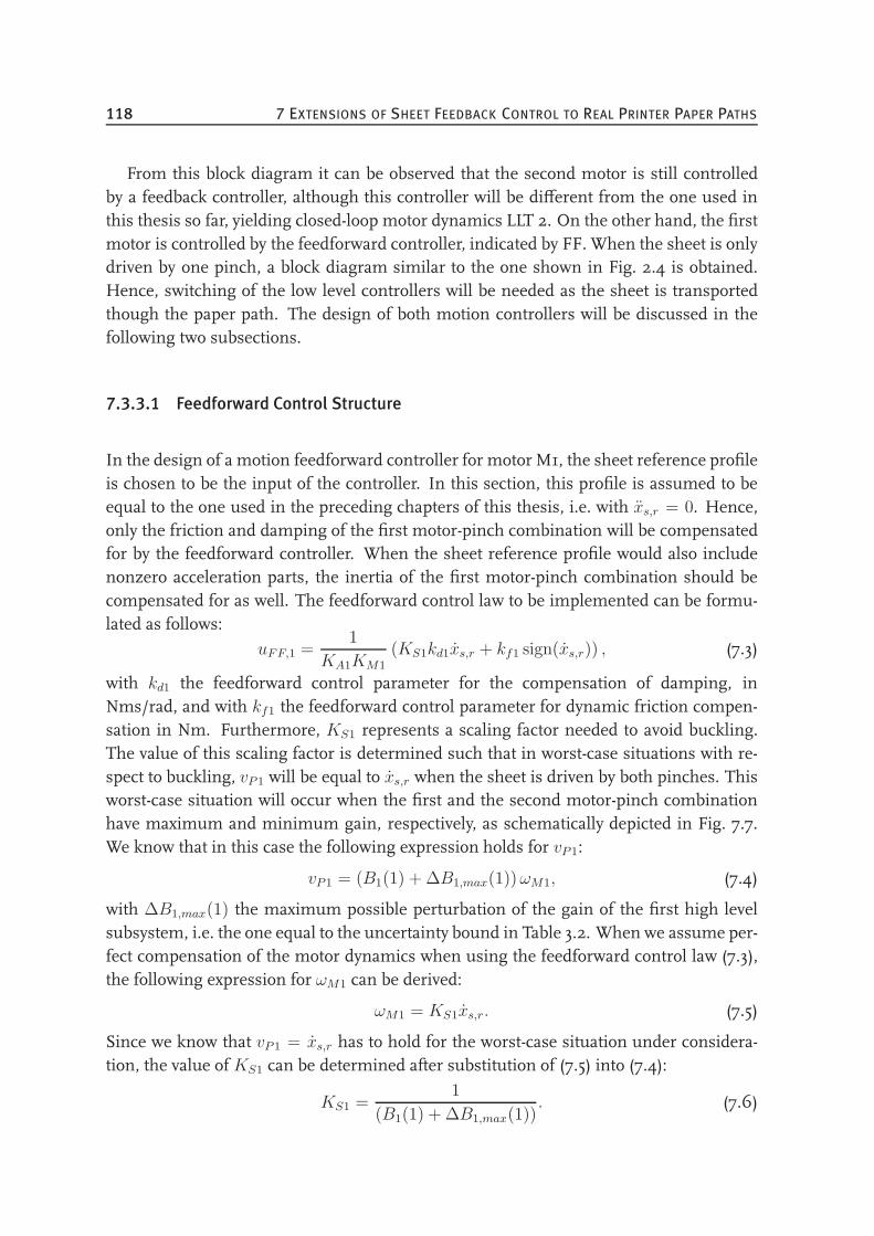
118 7 EXTENSIONS OF SHEET FEEDBACK CONTROL TO REAL PRINTER PAPER PATHS
From this block diagram it can be observed that the second motor is still controlledby a feedback controller, although this controller will be different from the one used inthis thesis so far, yielding closed-loop motor dynamics LLT 2. On the other hand, the firstmotor is controlled by the feedforward controller, indicated by FF. When the sheet is onlydriven by one pinch, a block diagram similar to the one shown in Fig. 2.4 is obtained.Hence, switching of the low level controllers will be needed as the sheet is transportedthough the paper path. The design of both motion controllers will be discussed in thefollowing two subsections.
7.3.3.1 Feedforward Control Structure
In the design of a motion feedforward controller for motor M1, the sheet reference profileis chosen to be the input of the controller. In this section, this profile is assumed to beequal to the one used in the preceding chapters of this thesis, i.e. with xs,r = 0. Hence,only the friction and damping of the first motor-pinch combination will be compensatedfor by the feedforward controller. When the sheet reference profile would also includenonzero acceleration parts, the inertia of the first motor-pinch combination should becompensated for as well. The feedforward control law to be implemented can be formu-lated as follows:
uFF,1 =1
KA1KM1(KS1kd1xs,r + kf1 sign(xs,r)) , (7.3)
with kd1 the feedforward control parameter for the compensation of damping, inNms/rad, and with kf1 the feedforward control parameter for dynamic friction compen-sation in Nm. Furthermore, KS1 represents a scaling factor needed to avoid buckling.The value of this scaling factor is determined such that in worst-case situations with re-spect to buckling, vP1 will be equal to xs,r when the sheet is driven by both pinches. Thisworst-case situation will occur when the first and the second motor-pinch combinationhave maximum and minimum gain, respectively, as schematically depicted in Fig. 7.7.We know that in this case the following expression holds for vP1:
vP1 = (B1(1) + ∆B1,max(1))ωM1, (7.4)
with ∆B1,max(1) the maximum possible perturbation of the gain of the first high levelsubsystem, i.e. the one equal to the uncertainty bound in Table 3.2. When we assume per-fect compensation of the motor dynamics when using the feedforward control law (7.3),the following expression for ωM1 can be derived:
ωM1 = KS1xs,r. (7.5)
Since we know that vP1 = xs,r has to hold for the worst-case situation under considera-tion, the value ofKS1 can be determined after substitution of (7.5) into (7.4):
KS1 =1
(B1(1) + ∆B1,max(1)). (7.6)
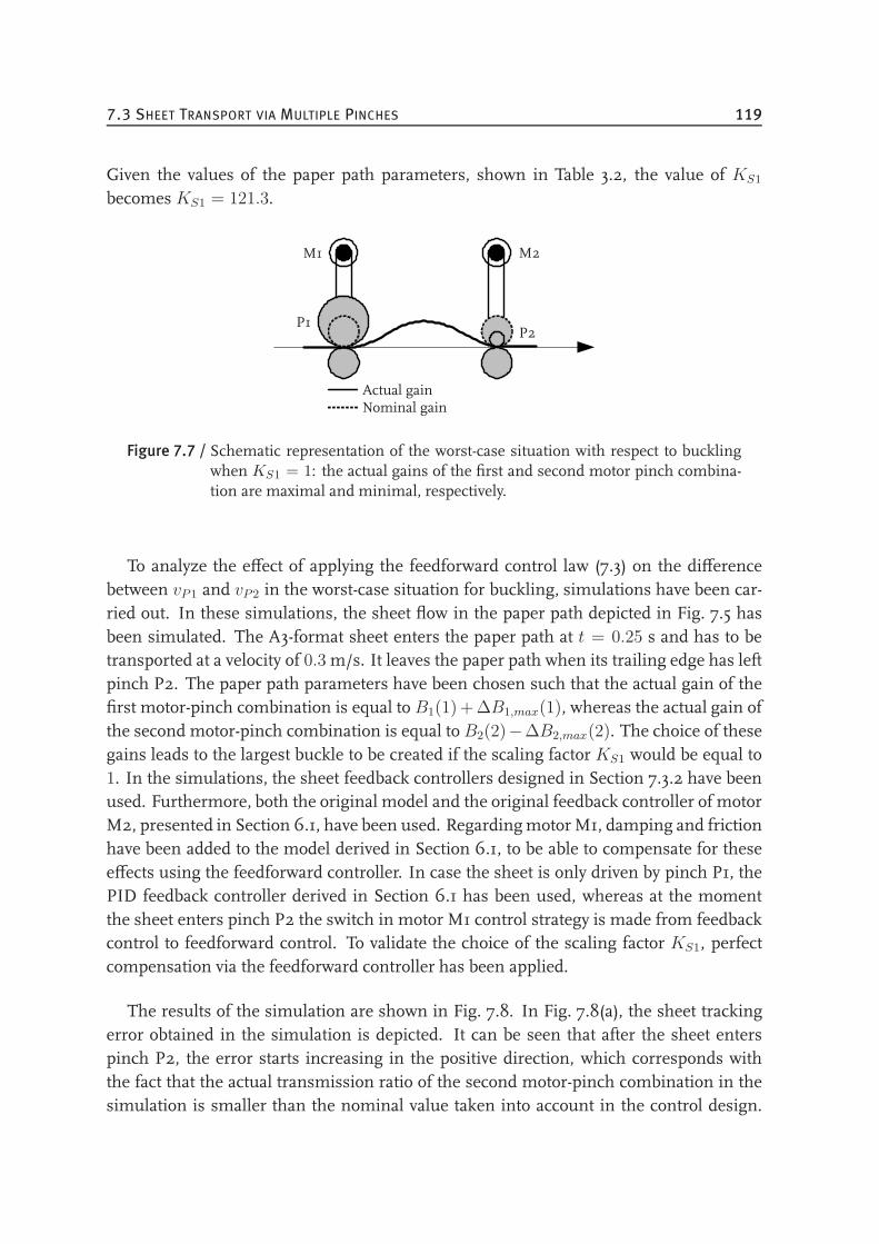
7.3 SHEET TRANSPORT VIA MULTIPLE PINCHES 119
Given the values of the paper path parameters, shown in Table 3.2, the value of KS1
becomes KS1 = 121.3.
Nominal gainActual gain
P1P2
M1 M2
Figure 7.7 / Schematic representation of the worst-case situation with respect to bucklingwhen KS1 = 1: the actual gains of the first and second motor pinch combina-tion are maximal and minimal, respectively.
To analyze the effect of applying the feedforward control law (7.3) on the differencebetween vP1 and vP2 in the worst-case situation for buckling, simulations have been car-ried out. In these simulations, the sheet flow in the paper path depicted in Fig. 7.5 hasbeen simulated. The A3-format sheet enters the paper path at t = 0.25 s and has to betransported at a velocity of 0.3 m/s. It leaves the paper path when its trailing edge has leftpinch P2. The paper path parameters have been chosen such that the actual gain of thefirst motor-pinch combination is equal to B1(1) + ∆B1,max(1), whereas the actual gain ofthe second motor-pinch combination is equal to B2(2)−∆B2,max(2). The choice of thesegains leads to the largest buckle to be created if the scaling factor KS1 would be equal to1. In the simulations, the sheet feedback controllers designed in Section 7.3.2 have beenused. Furthermore, both the original model and the original feedback controller of motorM2, presented in Section 6.1, have been used. Regardingmotor M1, damping and frictionhave been added to the model derived in Section 6.1, to be able to compensate for theseeffects using the feedforward controller. In case the sheet is only driven by pinch P1, thePID feedback controller derived in Section 6.1 has been used, whereas at the momentthe sheet enters pinch P2 the switch in motor M1 control strategy is made from feedbackcontrol to feedforward control. To validate the choice of the scaling factor KS1, perfectcompensation via the feedforward controller has been applied.
The results of the simulation are shown in Fig. 7.8. In Fig. 7.8(a), the sheet trackingerror obtained in the simulation is depicted. It can be seen that after the sheet enterspinch P2, the error starts increasing in the positive direction, which corresponds withthe fact that the actual transmission ratio of the second motor-pinch combination in thesimulation is smaller than the nominal value taken into account in the control design.
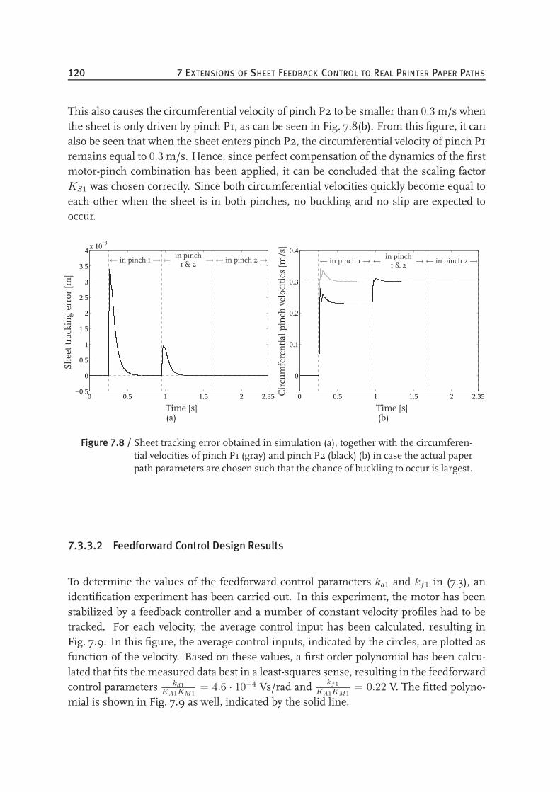
120 7 EXTENSIONS OF SHEET FEEDBACK CONTROL TO REAL PRINTER PAPER PATHS
This also causes the circumferential velocity of pinch P2 to be smaller than 0.3 m/s whenthe sheet is only driven by pinch P1, as can be seen in Fig. 7.8(b). From this figure, it canalso be seen that when the sheet enters pinch P2, the circumferential velocity of pinch P1remains equal to 0.3 m/s. Hence, since perfect compensation of the dynamics of the firstmotor-pinch combination has been applied, it can be concluded that the scaling factorKS1 was chosen correctly. Since both circumferential velocities quickly become equal toeach other when the sheet is in both pinches, no buckling and no slip are expected tooccur.
0 0.5 1 1.5 2 2.35−0.5
0
0.5
1
1.5
2
2.5
3
3.5
4x 10
−3
Time [s]
Sheettrackingerror[m
]
← in pinch 1→← in pinch1 & 2
→← in pinch 2→
(a)
0 0.5 1 1.5 2 2.35
0
0.1
0.2
0.3
0.4
Circumferentialpinch
velocities
[m/s]
Time [s]
← in pinch 1→ ← in pinch1 & 2
→← in pinch 2→
(b)
Figure 7.8 / Sheet tracking error obtained in simulation (a), together with the circumferen-tial velocities of pinch P1 (gray) and pinch P2 (black) (b) in case the actual paperpath parameters are chosen such that the chance of buckling to occur is largest.
7.3.3.2 Feedforward Control Design Results
To determine the values of the feedforward control parameters kd1 and kf1 in (7.3), anidentification experiment has been carried out. In this experiment, the motor has beenstabilized by a feedback controller and a number of constant velocity profiles had to betracked. For each velocity, the average control input has been calculated, resulting inFig. 7.9. In this figure, the average control inputs, indicated by the circles, are plotted asfunction of the velocity. Based on these values, a first order polynomial has been calcu-lated that fits themeasured data best in a least-squares sense, resulting in the feedforwardcontrol parameters kd1
KA1KM1= 4.6 · 10−4 Vs/rad and kf1
KA1KM1= 0.22 V. The fitted polyno-
mial is shown in Fig. 7.9 as well, indicated by the solid line.
7.3 SHEET TRANSPORT VIA MULTIPLE PINCHES 121
0 20 40 60 800
0.1
0.2
0.3
0.4
Average
control
inpu
t[V]
Velocity [rad/s]
Figure 7.9 / Average control input of motor M1 as a function of the angular motor velocity(circles), and the corresponding fitted first order polynomial (solid).
7.3.3.3 Feedback Control Design Results
The design of the feedback controller for motor M2, which is active when the sheet isdriven by both pinches, is based on the dynamics of the two motor-pinch combinationsthat are connected via the sheet. To identify these coupled dynamics, FRF measurementshave been carried out using the procedure presented in Section 6.1. During these mea-surements, motor M2, controlled by a low gain feedback controller, had to track a con-stant velocity. Since no control input was applied to motor M1, a pulling force was alwayspresent in the sheet, despite the addition of broadband noise to the output of the sec-ond motor controller, and the coupled dynamics could be identified. The results of theidentification procedure are reliable in the frequency range above the bandwidth of thecontrolled system, which was 10 Hz in this case, since in this range the coherence of themeasurement is good. This can be observed from Fig. 6.1, which shows the coherence ofthe sensitivity function, together with the FRF of the first motor-pinch combination. Inanalogy with Fig. 6.1, the decoupling of both the driven and the non-driven roller of pinchP2 manifest themselves as antiresonance-resonance pairs around 120 Hz and 200 Hz, re-spectively. The main difference between the FRF shown in Fig. 7.10 with respect to theones shown in Fig. 6.1 is the antiresonance-resonance pair in the frequency range be-tween 60 − 100 Hz, resulting from the decoupling of the first motor-pinch combination.
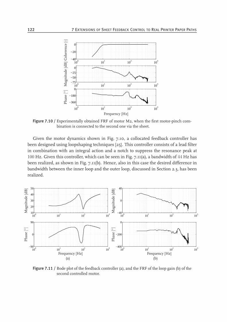
122 7 EXTENSIONS OF SHEET FEEDBACK CONTROL TO REAL PRINTER PAPER PATHS
100
101
102
103
−40
−20
0
100
101
102
103
−75
−50
−25
0
100
101
102
103
−360
−180
0
Coh
eren
ce[-]
Magnitude
[dB]
Phase
[]
Frequency [Hz]
Figure 7.10 / Experimentally obtained FRF of motor M2, when the first motor-pinch com-bination is connected to the second one via the sheet.
Given the motor dynamics shown in Fig. 7.10, a collocated feedback controller hasbeen designed using loopshaping techniques [25]. This controller consists of a lead filterin combination with an integral action and a notch to suppress the resonance peak at100 Hz. Given this controller, which can be seen in Fig. 7.11(a), a bandwidth of 44 Hz hasbeen realized, as shown in Fig. 7.11(b). Hence, also in this case the desired difference inbandwidth between the inner loop and the outer loop, discussed in Section 2.3, has beenrealized.
100
101
102
103
10
20
30
40
50
100
101
102
103
−90
0
90
Magnitude
[dB]
Phase
[]
Frequency [Hz](a)
100
101
102
103
−40
0
40
100
101
102
103
−400
−200
0
Magnitude
[dB]
Phase
[]
Frequency [Hz](b)
Figure 7.11 / Bode plot of the feedback controller (a), and the FRF of the loop gain (b) of thesecond controlled motor.
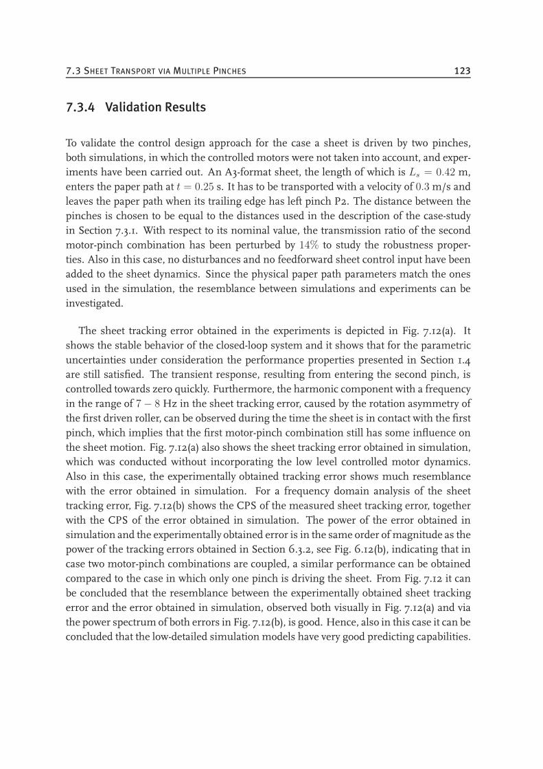
7.3 SHEET TRANSPORT VIA MULTIPLE PINCHES 123
7.3.4 Validation Results
To validate the control design approach for the case a sheet is driven by two pinches,both simulations, in which the controlled motors were not taken into account, and exper-iments have been carried out. An A3-format sheet, the length of which is Ls = 0.42 m,enters the paper path at t = 0.25 s. It has to be transported with a velocity of 0.3 m/s andleaves the paper path when its trailing edge has left pinch P2. The distance between thepinches is chosen to be equal to the distances used in the description of the case-studyin Section 7.3.1. With respect to its nominal value, the transmission ratio of the secondmotor-pinch combination has been perturbed by 14% to study the robustness proper-ties. Also in this case, no disturbances and no feedforward sheet control input have beenadded to the sheet dynamics. Since the physical paper path parameters match the onesused in the simulation, the resemblance between simulations and experiments can beinvestigated.
The sheet tracking error obtained in the experiments is depicted in Fig. 7.12(a). Itshows the stable behavior of the closed-loop system and it shows that for the parametricuncertainties under consideration the performance properties presented in Section 1.4are still satisfied. The transient response, resulting from entering the second pinch, iscontrolled towards zero quickly. Furthermore, the harmonic component with a frequencyin the range of 7 − 8 Hz in the sheet tracking error, caused by the rotation asymmetry ofthe first driven roller, can be observed during the time the sheet is in contact with the firstpinch, which implies that the first motor-pinch combination still has some influence onthe sheet motion. Fig. 7.12(a) also shows the sheet tracking error obtained in simulation,which was conducted without incorporating the low level controlled motor dynamics.Also in this case, the experimentally obtained tracking error shows much resemblancewith the error obtained in simulation. For a frequency domain analysis of the sheettracking error, Fig. 7.12(b) shows the CPS of the measured sheet tracking error, togetherwith the CPS of the error obtained in simulation. The power of the error obtained insimulation and the experimentally obtained error is in the same order of magnitude as thepower of the tracking errors obtained in Section 6.3.2, see Fig. 6.12(b), indicating that incase two motor-pinch combinations are coupled, a similar performance can be obtainedcompared to the case in which only one pinch is driving the sheet. From Fig. 7.12 it canbe concluded that the resemblance between the experimentally obtained sheet trackingerror and the error obtained in simulation, observed both visually in Fig. 7.12(a) and viathe power spectrum of both errors in Fig. 7.12(b), is good. Hence, also in this case it can beconcluded that the low-detailed simulation models have very good predicting capabilities.
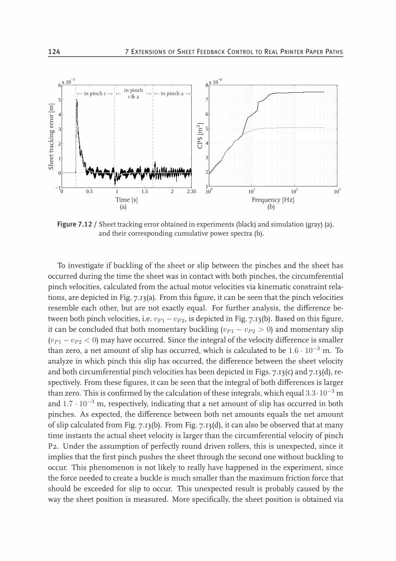
124 7 EXTENSIONS OF SHEET FEEDBACK CONTROL TO REAL PRINTER PAPER PATHS
0 0.5 1 1.5 2 2.35−1
0
1
2
3
4
5
6x 10
−3
Time [s]
Sheettrackingerror[m
]
← in pinch 1→ ← in pinch1 & 2
→ ← in pinch 2→
(a)
100
101
102
103
1
2
3
4
5
6
7
8x 10
−8
Frequency [Hz]CPS[m
2]
(b)
Figure 7.12 / Sheet tracking error obtained in experiments (black) and simulation (gray) (a),and their corresponding cumulative power spectra (b).
To investigate if buckling of the sheet or slip between the pinches and the sheet hasoccurred during the time the sheet was in contact with both pinches, the circumferentialpinch velocities, calculated from the actual motor velocities via kinematic constraint rela-tions, are depicted in Fig. 7.13(a). From this figure, it can be seen that the pinch velocitiesresemble each other, but are not exactly equal. For further analysis, the difference be-tween both pinch velocities, i.e. vP1−vP2, is depicted in Fig. 7.13(b). Based on this figure,it can be concluded that both momentary buckling (vP1 − vP2 > 0) and momentary slip(vP1 − vP2 < 0) may have occurred. Since the integral of the velocity difference is smallerthan zero, a net amount of slip has occurred, which is calculated to be 1.6 · 10−3 m. Toanalyze in which pinch this slip has occurred, the difference between the sheet velocityand both circumferential pinch velocities has been depicted in Figs. 7.13(c) and 7.13(d), re-spectively. From these figures, it can be seen that the integral of both differences is largerthan zero. This is confirmed by the calculation of these integrals, which equal 3.3 ·10−3 mand 1.7 · 10−3 m, respectively, indicating that a net amount of slip has occurred in bothpinches. As expected, the difference between both net amounts equals the net amountof slip calculated from Fig. 7.13(b). From Fig. 7.13(d), it can also be observed that at manytime instants the actual sheet velocity is larger than the circumferential velocity of pinchP2. Under the assumption of perfectly round driven rollers, this is unexpected, since itimplies that the first pinch pushes the sheet through the second one without buckling tooccur. This phenomenon is not likely to really have happened in the experiment, sincethe force needed to create a buckle is much smaller than the maximum friction force thatshould be exceeded for slip to occur. This unexpected result is probably caused by theway the sheet position is measured. More specifically, the sheet position is obtained via
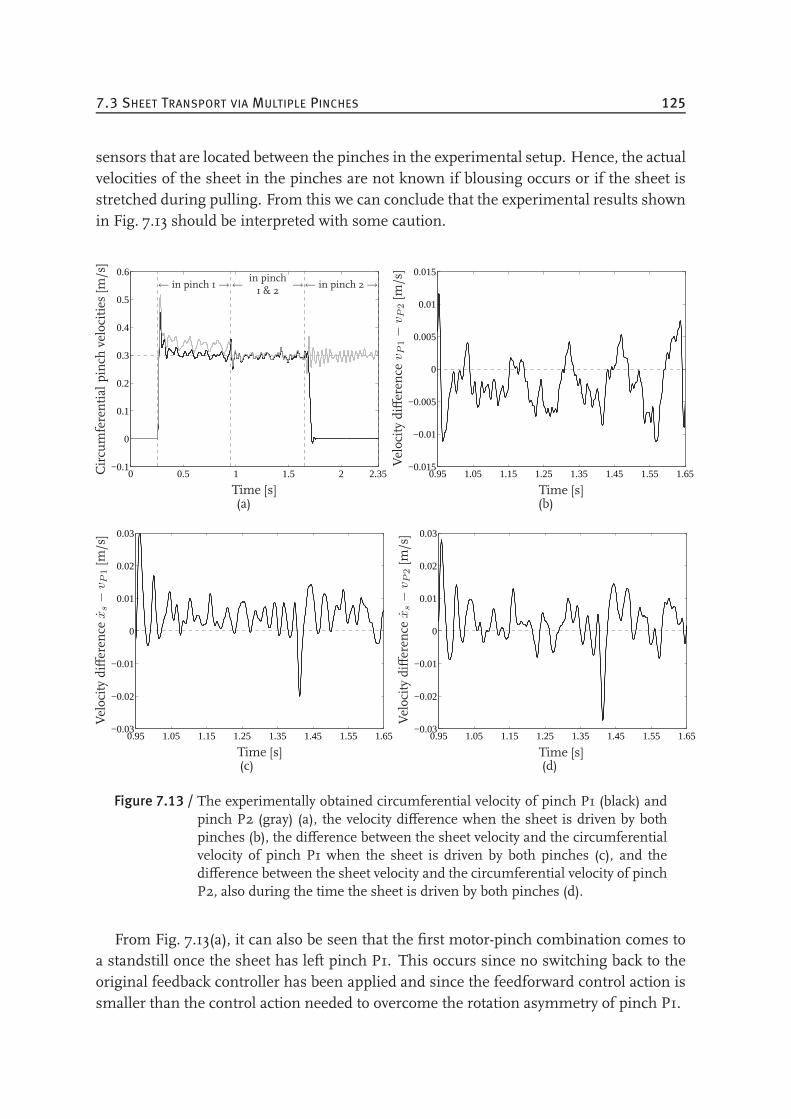
7.3 SHEET TRANSPORT VIA MULTIPLE PINCHES 125
sensors that are located between the pinches in the experimental setup. Hence, the actualvelocities of the sheet in the pinches are not known if blousing occurs or if the sheet isstretched during pulling. From this we can conclude that the experimental results shownin Fig. 7.13 should be interpreted with some caution.
0 0.5 1 1.5 2 2.35−0.1
0
0.1
0.2
0.3
0.4
0.5
0.6
Time [s]
Circumferential
pinch
velocities
[m/s]
← in pinch 1→← in pinch1 & 2
→← in pinch 2→
(a)
0.95 1.05 1.15 1.25 1.35 1.45 1.55 1.65−0.015
−0.01
−0.005
0
0.005
0.01
0.015
Time [s]
Velocitydifferen
cev
P1−
vP
2[m
/s]
(b)
0.95 1.05 1.15 1.25 1.35 1.45 1.55 1.65−0.03
−0.02
−0.01
0
0.01
0.02
0.03
Time [s]
Velocitydifferen
cex
s−
vP
1[m
/s]
(c)
0.95 1.05 1.15 1.25 1.35 1.45 1.55 1.65−0.03
−0.02
−0.01
0
0.01
0.02
0.03
Time [s]
Velocitydifferen
cex
s−
vP
2[m
/s]
(d)
Figure 7.13 / The experimentally obtained circumferential velocity of pinch P1 (black) andpinch P2 (gray) (a), the velocity difference when the sheet is driven by bothpinches (b), the difference between the sheet velocity and the circumferentialvelocity of pinch P1 when the sheet is driven by both pinches (c), and thedifference between the sheet velocity and the circumferential velocity of pinchP2, also during the time the sheet is driven by both pinches (d).
From Fig. 7.13(a), it can also be seen that the first motor-pinch combination comes toa standstill once the sheet has left pinch P1. This occurs since no switching back to theoriginal feedback controller has been applied and since the feedforward control action issmaller than the control action needed to overcome the rotation asymmetry of pinch P1.
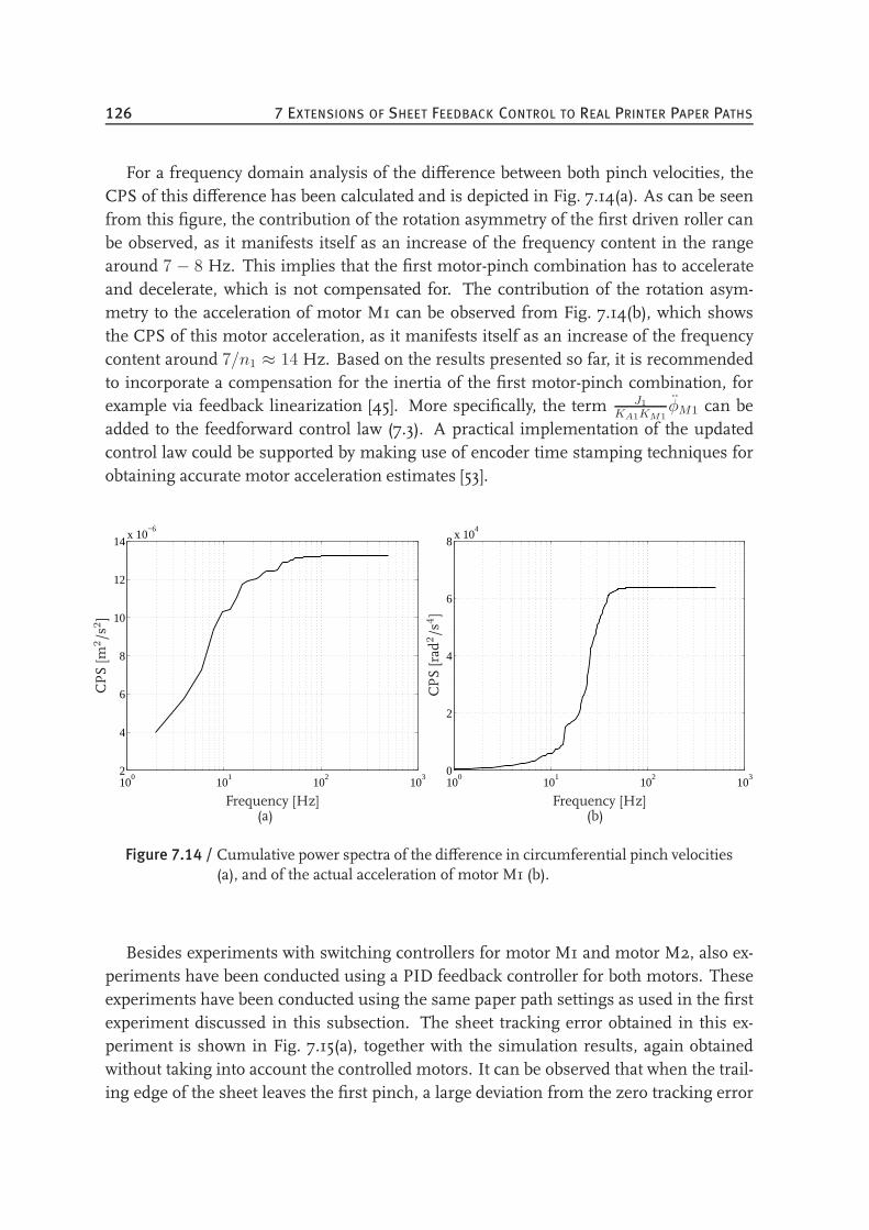
126 7 EXTENSIONS OF SHEET FEEDBACK CONTROL TO REAL PRINTER PAPER PATHS
For a frequency domain analysis of the difference between both pinch velocities, theCPS of this difference has been calculated and is depicted in Fig. 7.14(a). As can be seenfrom this figure, the contribution of the rotation asymmetry of the first driven roller canbe observed, as it manifests itself as an increase of the frequency content in the rangearound 7 − 8 Hz. This implies that the first motor-pinch combination has to accelerateand decelerate, which is not compensated for. The contribution of the rotation asym-metry to the acceleration of motor M1 can be observed from Fig. 7.14(b), which showsthe CPS of this motor acceleration, as it manifests itself as an increase of the frequencycontent around 7/n1 ≈ 14 Hz. Based on the results presented so far, it is recommendedto incorporate a compensation for the inertia of the first motor-pinch combination, forexample via feedback linearization [45]. More specifically, the term J1
KA1KM1φM1 can be
added to the feedforward control law (7.3). A practical implementation of the updatedcontrol law could be supported by making use of encoder time stamping techniques forobtaining accurate motor acceleration estimates [53].
100
101
102
103
2
4
6
8
10
12
14x 10
−6
Frequency [Hz]
CPS[m
2/s
2]
(a)
100
101
102
103
0
2
4
6
8x 10
4
Frequency [Hz]
CPS[rad
2/s
4]
(b)
Figure 7.14 / Cumulative power spectra of the difference in circumferential pinch velocities(a), and of the actual acceleration of motor M1 (b).
Besides experiments with switching controllers for motor M1 and motor M2, also ex-periments have been conducted using a PID feedback controller for both motors. Theseexperiments have been conducted using the same paper path settings as used in the firstexperiment discussed in this subsection. The sheet tracking error obtained in this ex-periment is shown in Fig. 7.15(a), together with the simulation results, again obtainedwithout taking into account the controlled motors. It can be observed that when the trail-ing edge of the sheet leaves the first pinch, a large deviation from the zero tracking error
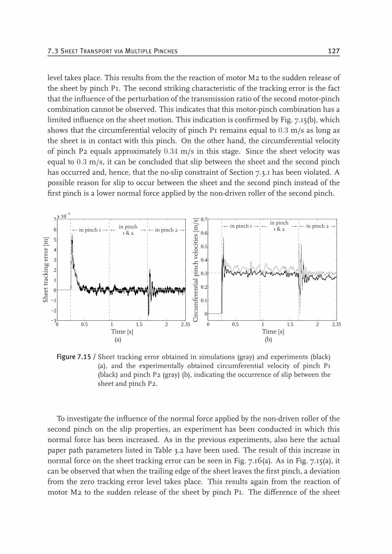
7.3 SHEET TRANSPORT VIA MULTIPLE PINCHES 127
level takes place. This results from the the reaction of motor M2 to the sudden release ofthe sheet by pinch P1. The second striking characteristic of the tracking error is the factthat the influence of the perturbation of the transmission ratio of the second motor-pinchcombination cannot be observed. This indicates that this motor-pinch combination has alimited influence on the sheet motion. This indication is confirmed by Fig. 7.15(b), whichshows that the circumferential velocity of pinch P1 remains equal to 0.3 m/s as long asthe sheet is in contact with this pinch. On the other hand, the circumferential velocityof pinch P2 equals approximately 0.34 m/s in this stage. Since the sheet velocity wasequal to 0.3 m/s, it can be concluded that slip between the sheet and the second pinchhas occurred and, hence, that the no-slip constraint of Section 7.3.1 has been violated. Apossible reason for slip to occur between the sheet and the second pinch instead of thefirst pinch is a lower normal force applied by the non-driven roller of the second pinch.
0 0.5 1 1.5 2 2.35−3
−2
−1
0
1
2
3
4
5
6
7x 10
−3
Time [s]
Sheettrackingerror[m
]
← in pinch 1→ ← in pinch1 & 2
→ ← in pinch 2→
(a)
0 0.5 1 1.5 2 2.35
0
0.1
0.2
0.3
0.4
0.5
0.6
0.7
Time [s]
Circumferentialpinch
velocities
[m/s]
← in pinch 1→ ← in pinch1 & 2
→ ← in pinch 2→
(b)
Figure 7.15 / Sheet tracking error obtained in simulations (gray) and experiments (black)(a), and the experimentally obtained circumferential velocity of pinch P1(black) and pinch P2 (gray) (b), indicating the occurrence of slip between thesheet and pinch P2.
To investigate the influence of the normal force applied by the non-driven roller of thesecond pinch on the slip properties, an experiment has been conducted in which thisnormal force has been increased. As in the previous experiments, also here the actualpaper path parameters listed in Table 3.2 have been used. The result of this increase innormal force on the sheet tracking error can be seen in Fig. 7.16(a). As in Fig. 7.15(a), itcan be observed that when the trailing edge of the sheet leaves the first pinch, a deviationfrom the zero tracking error level takes place. This results again from the reaction ofmotor M2 to the sudden release of the sheet by pinch P1. The difference of the sheet
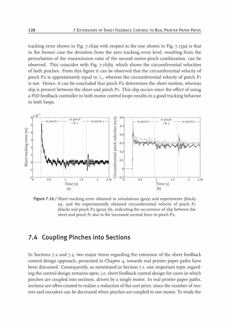
128 7 EXTENSIONS OF SHEET FEEDBACK CONTROL TO REAL PRINTER PAPER PATHS
tracking error shown in Fig. 7.16(a) with respect to the one shown in Fig. 7.15(a) is thatin the former case the deviation from the zero tracking error level, resulting from theperturbation of the transmission ratio of the second motor-pinch combination, can beobserved. This coincides with Fig. 7.16(b), which shows the circumferential velocitiesof both pinches. From this figure it can be observed that the circumferential velocity ofpinch P2 is approximately equal to xs, whereas the circumferential velocity of pinch P1is not. Hence, it can be concluded that pinch P2 determines the sheet motion, whereasslip is present between the sheet and pinch P1. This slip occurs since the effect of usinga PID feedback controller in both motor control loops results in a good tracking behaviorin both loops.
0 0.5 1 1.5 2 2.35−2
−1
0
1
2
3
4
5
6x 10
−3
Time [s]
Sheettrackingerror[m
]
← in pinch 1→ ← in pinch1 & 2
→ ← in pinch 2→
(a)
0 0.5 1 1.5 2 2.35−0.1
0
0.1
0.2
0.3
0.4
0.5
0.6
Time [s]
Circumferentialpinch
velocities
[m/s]
← in pinch 1→ ← in pinch1 & 2
→ ← in pinch 2→
(b)
Figure 7.16 / Sheet tracking error obtained in simulations (gray) and experiments (black)(a), and the experimentally obtained circumferential velocity of pinch P1(black) and pinch P2 (gray) (b), indicating the occurrence of slip between thesheet and pinch P1 due to the increased normal force in pinch P2.
7.4 Coupling Pinches into Sections
In Sections 7.2 and 7.3, two major items regarding the extension of the sheet feedbackcontrol design approach, presented in Chapter 4, towards real printer paper paths havebeen discussed. Consequently, as mentioned in Section 7.1, one important topic regard-ing the control design remains open, i.e. sheet feedback control design for cases in whichpinches are coupled into sections, driven by a single motor. In real printer paper paths,sections are often created to realize a reduction of the cost price, since the number of mo-tors and encoders can be decreased when pinches are coupled to one motor. To study the
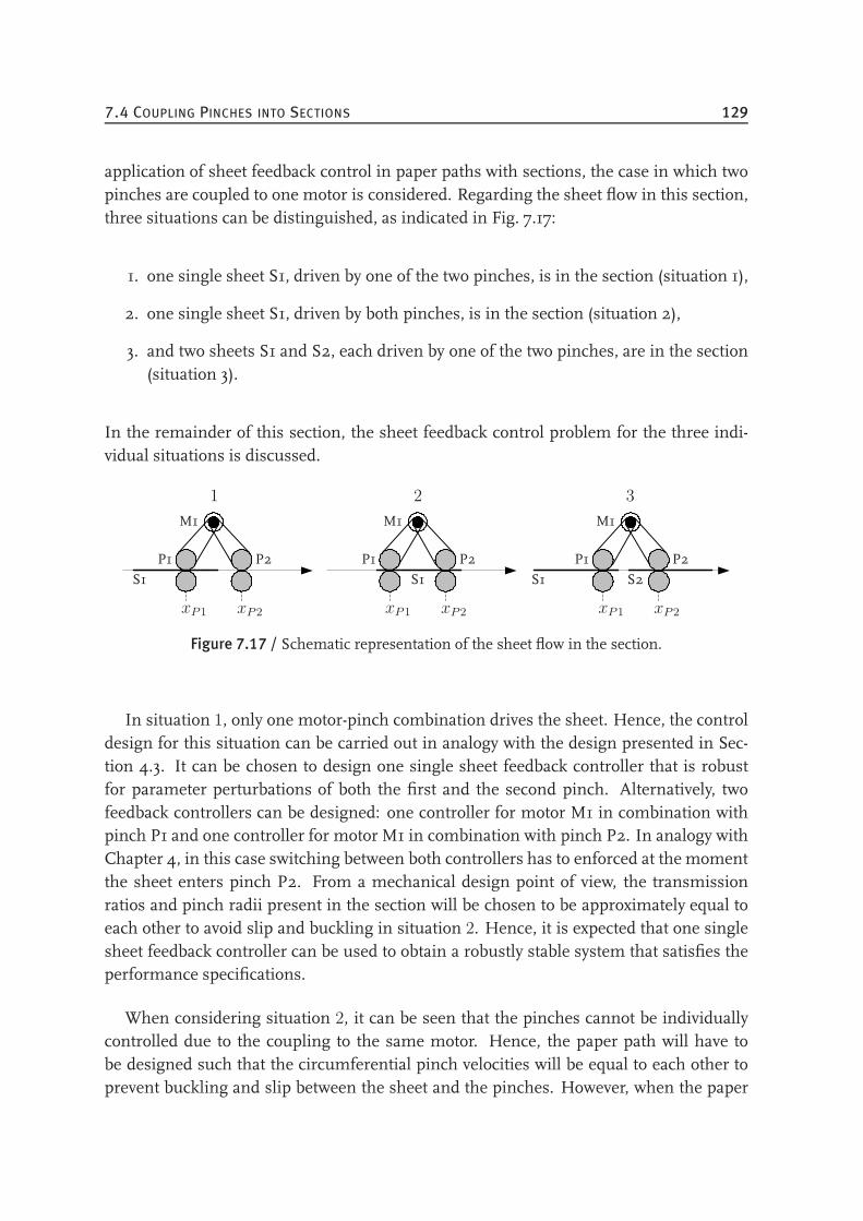
7.4 COUPLING PINCHES INTO SECTIONS 129
application of sheet feedback control in paper paths with sections, the case in which twopinches are coupled to one motor is considered. Regarding the sheet flow in this section,three situations can be distinguished, as indicated in Fig. 7.17:
1. one single sheet S1, driven by one of the two pinches, is in the section (situation 1),
2. one single sheet S1, driven by both pinches, is in the section (situation 2),
3. and two sheets S1 and S2, each driven by one of the two pinches, are in the section(situation 3).
In the remainder of this section, the sheet feedback control problem for the three indi-vidual situations is discussed.
1 2 3
M1M1M1
P1P1P1 P2P2P2
xP1xP1xP1 xP2xP2xP2
S1S1S1 S2
Figure 7.17 / Schematic representation of the sheet flow in the section.
In situation 1, only one motor-pinch combination drives the sheet. Hence, the controldesign for this situation can be carried out in analogy with the design presented in Sec-tion 4.3. It can be chosen to design one single sheet feedback controller that is robustfor parameter perturbations of both the first and the second pinch. Alternatively, twofeedback controllers can be designed: one controller for motor M1 in combination withpinch P1 and one controller for motor M1 in combination with pinch P2. In analogy withChapter 4, in this case switching between both controllers has to enforced at the momentthe sheet enters pinch P2. From a mechanical design point of view, the transmissionratios and pinch radii present in the section will be chosen to be approximately equal toeach other to avoid slip and buckling in situation 2. Hence, it is expected that one singlesheet feedback controller can be used to obtain a robustly stable system that satisfies theperformance specifications.
When considering situation 2, it can be seen that the pinches cannot be individuallycontrolled due to the coupling to the same motor. Hence, the paper path will have tobe designed such that the circumferential pinch velocities will be equal to each other toprevent buckling and slip between the sheet and the pinches. However, when the paper
130 7 EXTENSIONS OF SHEET FEEDBACK CONTROL TO REAL PRINTER PAPER PATHS
path parameters deviate from their nominal values, slip or buckling can in this case notbe prevented, unless mechanical solutions are applied. As mentioned in Section 7.3.1,examples of mechanical solutions are lifting of pinch P1 as soon as the sheet enters pinchP2 or equipping pinch P1 with a unidirectional bearing and designing the sheet referencevelocity such that it increases when the sheet enters pinch P2. Since these mechanicalsolutions support the decomposition of the control problem into two levels, the controldesign approach proposed in this thesis can still be applied. However, as already rec-ognized in Section 7.3.1, additional costs in the design are needed. If high level sheetfeedback control is applied without the mechanical adaptations, the paper path should bedesigned such that blousing can occur without damaging the sheet. On the other hand,slip between the sheet and one of the pinches cannot be prevented in case of parameterperturbations. However, if it is ensured that this slip occurs between the sheet and theupstream pinch by enforcing the largest normal force applied by the downstream pinch,the high level sheet feedback control design approach proposed in this thesis can be ap-plied. More specifically, if the downstream pinch determines the sheet motion and noslip occurs between this pinch and the sheet, the control problem can be decomposedinto two levels and a sheet feedback controller can be designed. An a posteriori perfor-mance analysis can be carried out to study the effect of slip in the upstream pinch on thetracking behavior.
In the third situation, multiple sheets present in the section cannot be controlled inde-pendently, since changing the motor reference velocity based on one of the sheet trackingerrors affects the motion of both sheets. In that case, the tracking requirements for in-dividual sheets must be adjusted since they cannot independently be realized in casemultiple sheets are in a single section. Hence, it should be decided based on which sheettracking error the motor reference velocity of the section should be calculated. One possi-bility is to add additional logic to the sheet feedback control level, which itself is designedusing the control design approach presented in Section 4.3, possibly using the extensionspresented in Sections 7.2 and 7.3. This design approach, which is based on one singlesheet, can be used since the sheet flow dynamics are identical for each sheet. However, anew model of the sheet flow dynamics will have to be designed, based on the paper pathconfiguration.
7.5 Evaluation
In this chapter, it has been shown that the systematic methodology for applying sheetfeedback control in a basic paper path, presented in Chapters 2 and 4, can also be appliedin paper paths equipped with a duplex loop and in cases in which sheets are driven bymultiple motor-pinch combinations. Furthermore, directions for solutions for cases in
7.5 EVALUATION 131
which pinches are coupled into sections are presented. Hence, the technical feasibilityof the sheet feedback control design approach has been proven, which opens the waytowards the integration and implementation in a real printer paper path. Regarding thisimplementation and integration step, a number of important subjects plays a role. First ofall, it should be investigated if additional elements present in the paper path, e.g. a regis-tration unit for sheet corrections in lateral and skewness direction, impose complicationsto the sheet feedback control design process. Furthermore, the reproducibility of themouse sensors should be improved in order to obtain accurate absolute sheet position in-formation, needed to realize the desired printing quality. An alternative for improving thereproducibility is making use of other contactless sheet position sensors. From a broaderperspective, another important subject is the integration of the high level control softwareinto the existing embedded control software. It is interesting to analyze the effect of thesynchronous sheet position updates on the predictability of the real-time software [42],in comparison with the asynchronous updates obtained by the I/O sheet sensors usedin current printer paper paths. Moreover, it is interesting to investigate to what extentthe presented approach results in an increase in computational effort, compared with thecurrent event-driven sheet feedback control approach.
Besides the integration and implementation of the sheet feedback control design ap-proach in a real printer paper path, the economical feasibility of the approach should beinvestigated. More specifically, it should be studied whether economic benefits of theapproach, e.g. the possible reduction of the paper path design time and the possible re-duction of the costs of the mechanical parts resulting from the decreased demands ontheir tolerances, are profitable with respect to the economic drawbacks, e.g. the increasedcosts resulting from the use of additional sheet sensors. A positive outcome of this studywill open the way to application of the sheet feedback control design approach in indus-trial printer development.

132
CHAPTER EIGHT
Conclusions and Recommendations
8.1 Conclusions . . . . . . . . . . . . . . . . . . . . . . . . . . . . . . . . . 133
8.2 Recommendations . . . . . . . . . . . . . . . . . . . . . . . . . . . . . . 135
8.1 Conclusions
In this thesis a systematic, model-based design methodology for controlling the longitu-dinal sheet flow in a printer paper path has been developed. In describing the sheet flowin the basic paper path case-study that was initially adopted, low-detailed, kinematic mod-els were used. In the derivation of these models, flexibilities between motors and pinchesand slip between sheets and pinches were assumed not to be present, as a result of whicha decoupling of the overall control problem into low level motor control and high levelsheet control became possible. The benefit of the resulting hierarchical control setupis the independent design of motor control and sheet control, resulting in a significantsimplification of the overall design problem.
For the design of the sheet feedback control loop, two approaches have been presented.In the first approach, the control design has been carried out based on the piecewise lin-ear nominal sheet flow model which was written in terms of its error dynamics. A dis-tinguishing feature with respect to the derivation of the error dynamics of linear systemswas the introduction of jump conditions describing the system behavior at the switch-ing boundary. Hence, unlike the linear case, a discontinuous, piecewise linear modelhas been obtained. Given this model, it was shown that to be able to define zero to be aglobally asymptotically stable equilibrium point of the system in the sense of Lyapunov,dependencies between a part of the controller parameters had to be introduced. Based on
133
134 8 CONCLUSIONS AND RECOMMENDATIONS
this observation, two types of controllers have been designed, yielding either a linear ora PWL, discontinuous closed-loop system. Stability analysis of both systems has yieldedmuch insight in the relation between the type of controller used and the type of Lyapunovfunction needed to prove the stability of this type of systems. In case parametric uncer-tainties are considered, it can be concluded that the control design approach presentedis not suitable, since in case of uncertainties it is not possible to define the origin to bea globally asymptotically stable equilibrium point of the error dynamics. Hence, controldesign for robustness is not possible. However, a posteriori analysis has been used toinvestigate the influence of parametric uncertainties on the tracking performance of thesystem. From this analysis it can be concluded that in case the sheet tracking error andthe sheet velocity error are zero before the sheet enters the next pinch, the controllerparameters do not influence the jump in the sheet velocity error resulting from the per-turbation of the system parameters. More specifically, in this case the performance guar-antees should be obtained from the mechanical design of the system, as the jumps areonly influenced by the paper path parameters.
The second control design approach is based on the high level sheet flow model itself.Using this approach, dynamic output feedback controllers for the switching dynamics athand are designed, taking into account parametric uncertainties into the control design.By combining linearH∞ control design techniques for the individual regimes of the sheetflow dynamics with stability and performance requirements for the overall switched sys-tem, robustness against parameter perturbations within prespecified bounds can be ob-tained. By using this approach, the closed-loop dynamics in each regime can be shapedaccording to the designer’s demands, and therefore this approach can be very well usedto solve the sheet feedback control problem.
The experiments performed on an experimental paper path setup, used for the prac-tical validation of both control design approaches, have shown that the desired trackingperformance can be realized, even when the system is subject to parameter perturbationswithin a prespecified bound. The experimental results for the basic paper path case-studyhave also shown that slip between the sheet and the pinches does not occur. Hence, theno-slip assumptionmade in themodeling process has been justified. Themost appealingoutcome of the validation experiments is the close resemblance between the experimen-tally obtained responses and the ones obtained in simulation. From this resemblance,it can be concluded that in case of the basic paper path case-study the combination ofsheet feedback controllers together with simple sheet flow models, that do not containthe closed-loop motor dynamics, are very well capable of predicting the sheet flow in re-ality. Hence, using these models in early stages of the design process has been justified.
With the experimental validation of the sheet feedback control design approaches, thedesign cycle is complete. The PWL modeling formalism and the controller synthesis tech-
8.2 RECOMMENDATIONS 135
niques, together with the supportive tools for the calculation of the controller gains and thesystematic method of applying these in combination with simulations and experimentshave resulted in the desired methodology for applying sheet feedback control in a basicprinter paper path. Because of the model-based character of this methodology, fast de-sign cycles can be realized, as the sheet flowmodel allows for an easy adaptation of modelparameters, pinch locations, etc. The modeling and control design can be carried out assoon as the first paper path design ideas are ready and the first sheet schedules have beendesigned. Hence, an early stage integration of the methodology in the paper path designprocess is possible. Based on these observations, the proposed approach is expected tocontribute to both a decrease of the development time and an increase of the predictabil-ity of the design process of the printer paper path, possibly resulting in a decrease of thedevelopment costs. With respect to the application of the systematic design methodologyto the printer case, it can be observed that performance does not depend that heavily onaccuratemechanics anymore. Hence, the robustness against disturbances and uncertain-ties might be increased and it may be possible to build less expensive printers with equalperformance. The application of sheet feedback control might also provide an increaseof the sheet handling capabilities. Consequently, the sheet flow might become more pre-dictable, especially in case disturbances and uncertainties are present in the paper path,which might result in an increase of the throughput.
Starting from the control design for the basic printer paper path, two extensions havebeen made towards real printer paper paths, i.e. modeling and control design in case thepaper path is equipped with a duplex loop for back-side printing, and sheet handling inwhich multiple motor-pinch combinations are driving a sheet. Regarding the latter ex-tension, the low level motor control loops have been adjusted to prevent buckling and slipfrom occurring. An alternative would have been to lift the upstream pinch or to use uni-directional bearings. However, by using the control approach as presented, no additionalexpenses are needed in the design of the sheet handling system. With the extensions pre-sented, the basis of a reusable, systematic design approach for sheet handling in printerpaper paths has been created, opening the way towards the integration and implementa-tion in a real paper path.
8.2 Recommendations
For future research, a few suggestions are considered to extend the work presented in thisthesis. These recommendations are divided into recommendations concerning the con-trol design approaches on the one hand, and recommendations regarding the integrationand implementation of sheet feedback control in a real paper path on the other hand.
136 8 CONCLUSIONS AND RECOMMENDATIONS
8.2.1 Recommendations for the Control Design Approaches
First of all, it is recommended to carry out additional research on the calculation of thecontroller parameters and the Lyapunov functions in Section 3.2.1.2. Currently, a ratherad-hoc approach is used, whereas more structured approaches are desirable. Reformula-tion of the control problem in terms of LMIs or BMIs might be a proper starting pointfor future research.
Secondly, it is recommended to perform additional research on the possible benefitsof sheet feedback controllers that result in partial linearization of the sheet dynamics.Compared with feedback controllers that yield a linear closed-loop system, the design ofthis type of controllers allows more freedom in the choice of the controller parameters.This could result in an improved behavior of the system, such as an improvement ofthe performance index containing the control input, or in the introduction of additionalcharacteristics, such as the possibility to design for different control bandwidths in thevarious subsystems.
A third recommendation regarding the control design presented in Chapter 3 is to in-vestigate the possibility of incorporating additional dynamics in the sheet feedback con-trollers. This way, a high frequency roll-off can be included in the controllers, as done inSections 4.2 and 4.3. Furthermore, available a priori knowledge on frequency ranges inwhich disturbances are likely to be present can be taken into account in the design.
Since so far only first order reference profiles have been considered in the controldesign approach presented in Chapter 3, a final recommendation concerning this chapteris to carry out sheet feedback control design based on sheet flow models in error spacethat are derived from more realistic sheet reference profiles.
Considering the practical implementation of the control design approaches, in Chap-ter 5 it was observed that an exact continuous absolute position measurement of thesheets in the paper path cannot be obtained using the current implementation of themouse sensors in the experimental setup. Therefore, more research on determining theabsolute sheet position, needed to realize the desired printing quality, will have to be car-ried out before implementing continuous sheet feedback control in a real paper path.One could think of, for example, improving the reproducibility of the mouse sensors orthe exploration of other possibilities for contactless sheet position measurement.
As far as extensions of sheet feedback control design for real printer paper paths areconcerned, two main recommendations can be given. First of all, in case a single sheetis driven by two pinches, more analysis on the occurrence of slip between the sheet andone of the pinches should be carried out. Moreover, the effect of these slip properties onthe low level control design for the upstreammotor should be explored.
8.2 RECOMMENDATIONS 137
The second recommendation concerning the extensions to real printer paper pathsencompasses sheet flow modeling and control design for cases in which pinches arecoupled into sections, driven by a single motor. Starting from the initial ideas on thistopic presented in Section 7.4, the modeling, control design, and validation should beconsidered in more detail.
8.2.2 Recommendations for Integration and Implementation
Also with respect to the integration and implementation of sheet feedback control in a realpaper path and in the paper path design process a few recommendations can be given.First of all, the integration of the high level control software into the existing embeddedcontrol software should be investigated. More specifically, since the current implemen-tation of discrete-event sheet controllers results in asynchronous updates of the sheetposition information, whereas using the approach presented in this thesis synchronousupdates are obtained, it is interesting to analyze if the predictability of the real-time soft-ware has increased. Moreover, it is interesting to investigate to what extent the presentedapproach results in an increase in computational effort.
Secondly, the economical feasibility of the approach should be investigated. Morespecifically, it should be studied whether the economic benefits of the approach, e.g. thepossible reduction of the paper path development time and the possible reduction of thecosts of the mechanical parts resulting from the decreased demands on their tolerances,are profitable with respect to the economic drawbacks, e.g. the increased costs result-ing from the use of optical mouse sensors, the additional wiring needed, and possibleincreased maintenance sensibility.
With respect to the economical feasibility, a few additional recommendations can begiven. First of all, the possibilities of using a sheet position estimation algorithm basedon the information obtained from the optical I/O sheet sensors already present in mostprinter paper paths is an interesting option to be investigated. Hence, the additional costson extra sheet sensors can be saved. As an alternative, the use of high level sheet sensorsfor motor control purposes can be investigated. This way, position encoders at the motorshafts are not needed anymore and a non-collocated control setup is obtained that can beused for controlling the sheets. The benefit of using only one type of sensors for controlis again a decrease of the printer’s cost price.
A final recommendation results from the fact that the use of stepper motors is becom-ing a serious option in printer paper path design [76]. Hence, it would be interesting toexamine the possibilities of applying sheet feedback control as proposed in this thesis in

138 8 CONCLUSIONS AND RECOMMENDATIONS
paper paths equipped with stepper motors. As the no-slip assumptions in the modelingprocess can still be made and since these stepper motors are controlled in a open-loopfashion, it is expected that this type of motors also supports the decoupling of the sheethandling control problem into high level sheet control and low level motor control.
APPENDIX A
Linearizing Change of Variables
The first step in the linearizing change of variables is the partitioning of P and P−1 as
P =
[Y NNT ∗
],P−1 =
[X MMT •
], (A.1)
where X and Y are n × n symmetric matrices, with n the number of states of the aug-mented plant. In (A.1), ∗ and • represent matrices satisfying
PP−1 =
[Y X +NMT YM +N•NTX + ∗MT NTM + ∗•
]= I. (A.2)
From (A.2) we know that P
(XMT
)=
(I0
), which leads to
PΠ1 = Π2, (A.3)
with Π1 =
[X IMT 0
]and Π2 =
[I Y0 NT
]. Next, the following change of controller
variables is defined:
Ai = NAK,iMT +NBK,iCv,iX + Y Bu,iCK,iM
T + Y (Ai +Bu,iDK,iCv,i)X
Bi = NBK,i + Y Bu,iDK,i
Ci = CK,iMT +DK,iCv,iX
Di = DK,i
, i ∈ I.
(A.4)The motivation for this transformation lies in the following identities, that are derived
139
140 A LINEARIZING CHANGE OF VARIABLES
from (A.3), (A.4), and (4.11):
ΠT1 PAiΠ1 = ΠT
2 AiΠ1
=
(Ai +Bu,iDK,iCv,i)X++Bu,iCK,iM
T Ai +Bu,iDK,iCv,i
Y (Ai +Bu,iDK,iCv,i)X + Y Bu,iCK,iMT+
+NBK,iCv,iX +NAK,iMT
Y (Ai +Bu,iDK,iCv,i) ++NBK,iCv,i
=
[AiX +Bu,iCi Ai +Bu,iDiCv,i
Ai Y Ai + BiCv,i
], i ∈ I (A.5)
ΠT1 PBi = ΠT
2 Bi
=
[Bw,i +Bu,iDK,iDvw,i
Y (Bw,i +Bu,iDK,iDvw,i) +NBK,iDvw,i
]
=
[Bw,i +Bu,iDiDvw,i
Y Bw,i + BiDvw,i
], i ∈ I (A.6)
CiΠ1 =[Cz,iX +Dzu,iDK,iCv,iX +Dzu,iCK,iM
T Cz,i +Dzu,iDK,iCv,i]
=[Cz,iX +Dzu,iCi Cz,i +Dzu,iDiCv,i
], i ∈ I. (A.7)
Pre- and postmultiplication of (4.19) with ΠT1 and Π1, respectively, results in (4.21):
0 ≺ ΠT1 PΠ1 = ΠT
1 Π2 =
[X II Y
]. (A.8)
Furthermore, pre- and postmultiplication of the analysis LMI (4.20) with diag(ΠT1 , I, I)
and diag(Π1, I, I), respectively, yields
0 ≻
ΠT
1 ATi PΠ1 + ΠT
1 PAiΠ1 ΠT1 PBi ΠT
1 CTi
BTi PΠ1 −γI DTi
CiΠ1 Di −γI
. (A.9)
Substitution of (A.4)-(A.7) into (A.9) yields the synthesis LMI (4.22).
Bibliography
[1] AVAGO TECHNOLOGIES. ADNB-6011-EV and ADNB-6012-
EV High Performance Laser Mouse Bundles (Data Sheet).http://www.avagotech.com/assets/downloadDocument.do?id=13561.
[2] BANNER ENGINEERING. http://www.bannerengineering.com.
[3] BECKERS, J.M.J., HEEMELS, W.P.M.H., BUKKEMS, B.H.M., and MULLER, G.J.Effective Industrial Modeling for High-Tech Systems: The Example of Happy Flow.In Proc. of the 17th Symposium International Council on Systems Engineering (INCOSE).Orlando, Florida, USA, 2007 (accepted).
[4] BELL, D., BOBROW, D., FALKENHAINER, B., FROMHERZ, M., SARASWAT, V., andSHIRLEY, M. RAPPER: The Copier Modeling Project. In Int. Workshop on Qualitative
Reasoning about Physical Systems. Nara, Japan, 1994, pp. 1–12.
[5] BOSGRA, O.H., KWAKERNAAK, H., and MEINSMA, G. Design Methods for Control
Systems. Lecture notes for the DISC course, Dutch Institute of Systems and Control,2003.
[6] BOYD, S., EL GHAOUI, L., FERON, E., and BALAKRISHNAN, V. Linear Matrix In-
equalities in System and Control Theory. Volume 15 of SIAM Studies in Applied Math-ematics, Philadelphia, PA, USA, June 1994.
[7] BUEDE, D.M. Engineering Design of Systems - Models and Methods. John Wiley &Sons, Inc., New York, NY, USA, 2000.
[8] BUKKEMS, B.H.M., DE BEST, J.J.T.H., VAN DE MOLENGRAFT, M.J.G., and STEIN-BUCH, M. Robust Piecewise Linear Sheet Control in a Printer Paper Path. In Proc. of
the 2nd IFAC Conference on Analysis and Design of Hybrid Systems (ADHS’06). 2006,pp. 142–147.
141
142 BIBLIOGRAPHY
[9] BUKKEMS, B.H.M., SANDEE, J.H., BECKERS, J.M.J., YUAN, Z., VAN DER WIJST,B., and VAN DE MOLENGRAFT, M.J.G. A Case-Study in Multidisciplinary Modelingof Dynamic Embedded Systems. In Proc. of Mechatronics and Robotics 2004 (MechRob
2004). Aken, Germany, 2004, pp. 26–31.
[10] BUKKEMS, B.H.M., VAN DE MOLENGRAFT, M.J.G., HEEMELS, W.P.M.H., VAN DE
WOUW, N., and STEINBUCH, M. A Piecewise Linear Approach Towards Sheet Con-trol in a Printer Paper Path. In Proc. of the American Control Conference 2006. 2006,pp. 1315–1320.
[11] CHEN, M., ZHU, C.R., and FENG, G. Linear-matrix-inequality-based approach toH∞ controller synthesis of uncertain continuous-time piecewise linear systems. IEEProc.-Control Theory Appl., vol. 151(3): (2004), pp. 295–300.
[12] CLOET, C. A Mechatronics Approach to Copier Paperpath Design. Ph.D. thesis, Uni-versity of California Berkeley, CA, USA, 2001.
[13] CLOET, C., KRUCINSKI, M., HOROWITZ, R., and TOMIZUKA, M. A Hybrid ControlScheme for a Copier Paper Path. In Proc. of the American Control Conference. SanDiego, CA, USA, 1999, pp. 2114–2118.
[14] CLOET, C., KRUCINSKI, M., TOMIZUKA, M., HOROWITZ, R., and LI, P. IntersheetSpacing Control and Controllability of a Copier Paper Path. In Proc. of the 1998 IEEE
International Conference on Control Applications. Trieste, Italy, 1998, pp. 726–730.
[15] CLOET, C., TOMIZUKA, M., and HOROWITZ, R. Design Requirements and Refer-ence Trajectory Generation for a Copier Paperpath. In Proc. of the 2001 IEEE/ASME
International Conference on Advanced Intelligent Mechatronics. 2001, pp. 911–916.
[16] CLOOSTERMAN, M.B.G., VAN DE WOUW, N., HEEMELS, W.P.M.H., and NIJMEI-JER, H. Robust Stability of Networked Control Systems with Time-Varying Network-Induced Delays. In Proc. of the 45th IEEE Conference on Decision and Control. SanDiego, California, USA, 2006, pp. 4980–4985.
[17] DAMEN, A. and WEILAND, S. Robust Control. Lecture notes for the course RobustControl (5P430), Technische Universiteit Eindhoven, 2001.
[18] DE BEST, J.J.T.H., BUKKEMS, B.H.M., VAN DE MOLENGRAFT, M.J.G., and STEIN-BUCH, M. Piecewise Linear Sheet Control in an H∞ Framework. In IEEE Multi-
conference on Systems and Control (MSC2007). Singapore, 2007 (accepted).
[19] DECARLO, R.A., BRANICKY, M.S., PETTERSSON, S., and LENNARTSON, B. Per-spectives and Results on the Stability and Stabilizability of Hybrid Systems. Proc.
IEEE, vol. 88(7): (2000), pp. 1069–1082.
BIBLIOGRAPHY 143
[20] DOYLE, J.C., PACKARD, A., and ZHOU, K. Review of LFTs, LMIs, and µ. In Proc.
of the 30th IEEE Conference on Decision and Control. Brighton, England, 1991, pp.1227–1232.
[21] EMBEDDED SYSTEMS INSTITUTE. Summary of the Boderc Project Plan.http://www.esi.nl/.
[22] FENG, G. Controller Design and Analysis of Uncertain Piecewise-Linear Systems.IEEE Trans. Circuits Syst. I, vol. 49(2): (2002), pp. 224–232.
[23] FENG, G., LU, G.P., and ZHOU, S.S. An Approach to H∞ Controller Synthesisof Piecewise Linear Systems. Communications in Information and Systems, vol. 2(3):(2002), pp. 245–254.
[24] FLORESCU, O., VOETEN, J.P.M., and CORPORAAL, H. A unified model for analy-sis of real-time properties. In Proc. of the 1st International Symposium on Leveraging
Applications of Formal Methods (ISoLa 2004). Paphos, Cyprus, 2004, pp. 220–227.
[25] FRANKLIN, G.F., POWELL, J.D., and EMAMI-NAEINI, A. Feedback control of dynamic
systems. Prentice Hall, Upper Saddle River, New Jersey, USA, 2002.
[26] FRERIKS, H.J.M., HEEMELS, W.P.M.H., MULLER, G.J., and SANDEE, J.H. On theSystematic Use of Budget-Based Design. In Proc. of the 16th symposium International
Council on Systems Engineering (INCOSE). Orlando, Florida, USA, 2006.
[27] FROMHERZ, M.P., CRAWFORD, L.S., and HINDI, H.A. Coordinated Controlfor Highly Reconfigurable Systems. In Hybrid Systems: Computation and Control
(HSCC) 2005. Zurich, Switzerland, 2005, pp. 1–24.
[28] GAHINET, P., NEMIROVSKI, A., LAUB, A.J., and CHILALI, M. LMI Control Toolbox
for Use with Matlab. The Mathworks Inc., Natick, MA, USA, May 1995.
[29] GAHINET, P. Explicit Controller Formulas for LMI-based H∞ Synthesis. Automat-
ica, vol. 32(7): (1996), pp. 1007–1014.
[30] GAHINET, P. and APKARIAN, P. A Linear Matrix Inequality Approach to H∞ Con-trol. Int. J. of Robust and Nonlinear Control, vol. 4: (1994), pp. 421–448.
[31] GUPTA, V., SARASWAT, V.A., and STRUSS, P. A model of a Photocopier Paper Path.In Proc. of the 2nd IJCAI Workshop on Engineering Problems for Qualitative Reasoning.1995.
[32] GUPTA, V. and STRUSS, P. Modeling a Copier Paper Path: A Case Study in Model-ing Transportation Processes. In Proc. of the 9th Workshop on Qualitative Reasoning.Amsterdam, The Netherlands, 1995.
144 BIBLIOGRAPHY
[33] HAMBY, E.S. and GROSS, E.M. A Control-Oriented Survey of Xerographic Systems:Basic Concepts to New Frontiers. In Proc. of the American Control Conference. Boston,MA, USA, 2004, pp. 2615–2620.
[34] HANG, C.C., LOH, A.P., and VASNANI, V.U. Relay Feedback Auto-Tuning of Cas-cade Controllers. IEEE Trans. Contr. Syst. Technol., vol. 2(1): (1994), pp. 42–45.
[35] HASSIBI, A. and BOYD, S. Quadratic Stabilization and Control of Piecewise-LinearSystems. In Proc. of the American Control Conference. Philadelphia, PA, USA, 1998,pp. 3659–3664.
[36] HEEMELS, W.P.M.H., MULLER, G.J., and VAN DEN BOSCH, P.F.A. Boderc: Model-
Based Design of High-Tech Systems (Chapter 1). Embedded Systems Institute, Eind-hoven, The Netherlands, 2006.
[37] HEEMELS, W.P.M.H., SOMERS, L., VAN DEN BOSCH, P.F.A., MULLER, G.J.,YUAN, Z., VAN DER WIJST, B., and VAN DEN BRAND, A. The Use of the Key DriverTechnique in the Design of Copiers. In Proc. of the International Conference on Soft-
ware and Systems Engineering and their Applications (ICSSEA). Paris, France, 2006.
[38] HEEMELS, W.P.M.H., VAN DE WAAL, E., and MULLER, G.J. A Multi-Disciplinaryand Model-Based DesignMethodology for High-Tech Systems. In Proc. of the Confer-
ence on System Engineering (CSER). Los Angeles, CA, USA, 2006.
[39] HENZINGER, T.A. The Theory of Hybrid Automata. In Proc. of the 11th Symposium
on Logic in Computer Science (LICS ’96). New Brunswick, New Jersey, USA, 1996,pp. 278–292.
[40] HINDI, H.A., CRAWFORD, L.S., and FROMHERZ, M.P.J. Synchronization of StateBased Control Processes with Delayed and Asynchronous Measurements. In Proc. of
the 44th IEEE Conference on Decision and Control and the European Control Conference
2005. Sevilla, Spain, 2005, pp. 6370–6375.
[41] HOL, C.W.J. Structured Controller Synthesis for Mechanical Servo-Systems; Algorithms,
Relaxations and Optimality Certificates. Ph.D. thesis, Delft University of Technology,Delft, The Netherlands, 2006.
[42] HUANG, J. Predictability in Real-Time Software Design. Ph.D. thesis, TechnischeUniversiteit Eindhoven, Eindhoven, The Netherlands, 2005.
[43] INCOSE. What is Systems Engineering? http://www.incose.org/practice/
whatissystemseng.aspx.
[44] JOHANSSON, M. and RANTZER, A. Computation of Piecewise Quadratic LyapunovFunctions for Hybrid Systems. IEEE Trans. Automat. Contr., vol. 43(4): (1998), pp.555–559.
BIBLIOGRAPHY 145
[45] KHALIL, H.K. Nonlinear Systems. Prentice Hall, Upper Saddle River, New Jersey,USA, 2002.
[46] KRUCINSKI, M. Feedback Control of Photocopying Machinery. Ph.D. thesis, Universityof California Berkeley, CA, USA, 2000.
[47] KRUCINSKI, M., CLOET, C., HOROWITZ, R., TOMIZUKA, M., and LI, P. Asyn-chronous Observer for a Copier Paper Path. In Proc. of the 37th IEEE Conference on
Decision and Control. Tampa, Florida, USA, 1998, pp. 2611–2612.
[48] KRUCINSKI, M., CLOET, C., HOROWITZ, R., TOMIZUKA, M., and LI, P. Inter-object Spacing Control and Controllability of a Manufacturing Transportation Sys-tem. In Proc. of the American Control Conference. Philadelphia, Pennsylvania, USA,1998, pp. 1259–1265.
[49] LAMBRECHTS, P.F. The Application of Robust Control Theory Concepts to Mechanical
Servo Systems. Ph.D. dissertation, Delft University of Technology, 1990.
[50] LEE, Y. and PARK, S. PID Controller Tuning To Obtain Desired closed-loop Re-sponses for Cascade Control Systems. Ind. Eng. Chem. Res., vol. 37(5): (1998), pp.1859–1865.
[51] LOGITECH. Logitech G5 Laser Mouse. http://www.logitech.com/index.cfm/
products/details/NL/EN,CRID=2464,CONTENTID=10715.
[52] MAAS, J.W.L.H. Sheet FlowModeling in a Printer Paper Path. Department of Mechan-ical Engineering, Technische Universiteit Eindhoven, Eindhoven, The Netherlands,2006.
[53] MERRY, R.J.E., VAN DE MOLENGRAFT, M.J.G., and STEINBUCH, M. Error Model-ing and Improved Position Estimation for Optical Incremental Encoders by meansof Time Stamping. In Proc. of the American Control Conference. New York City, USA,2007 (accepted).
[54] POLITECNICO DI MILANO - DIPARTIMENTO DI INGEGNERIA AEROSPAZIALE. RTAI- the RealTime Application Interface for Linux. https://www.rtai.org/.
[55] POTTS, C. Software-engineering Research Revisited. IEEE Software, vol. 10(5):(1993), pp. 19–28.
[56] RAI, S. and JACKSON, W.B. A Hybrid Hierarchical Control Architecture for PaperTransport Systems. In Proc. of the 37th IEEE Conference on Decision and Control.Tampa, Florida, USA, 1998, pp. 4249–4250.
[57] RANTZER, A. and JOHANSSON, M. Piecewise Linear Quadratic Optimal Control.IEEE Trans. Automat. Contr., vol. 45(4): (2000), pp. 629–637.
146 BIBLIOGRAPHY
[58] REPENNING, N.P. Understanding Fire Fighting in New Product Development. Jour-nal of Product Innovation Management, vol. 18(5): (2001), pp. 285–300.
[59] RODRIGUES, L., HASSIBI, A., andHOW, J.P. Output Feedback Controller Synthesisfor Piecewise-Affine SystemwithMultiple Equilibria. In Proc. of the American Control
Conference. Chicago, Illinois, USA, 2000, pp. 1784–1789.
[60] SAKAMURA, K. and SUGIE, T. Trajectory tracking control of bimodal piecewiseaffine systems. Int. J. of Control, vol. 78(16): (2005), pp. 1314–1326.
[61] SANCHEZ, R., ERGUETA, E., FINE, B., HOROWITZ, R., TOMIZUKA, M., and KRU-CINSKI, M. A Mechatronic Approach to Full Sheet Control Using Steer-able Nips.In Proc. of the 4th IFAC-Symposium on Mechatronic Systems. Heidelberg, Germany,2006, pp. 277–282.
[62] SANCHEZ, R., HOROWITZ, R., and TOMIZUKA, M. Paper Sheet Control UsingSteerable Nips. In Proc. of the American Control Conference. Boston, Massachusetts,USA, 2004, pp. 482–487.
[63] SANCHEZ, R., HOROWITZ, R., TOMIZUKA, M., and SIMIC, S.N. Full Paper SheetControl Using Hybrid Automata. In Hybrid Systems: Computation and Control. Vol.
2993 of Lecture Notes in Computer Science. Berlin, Germany, 2004, pp. 523–538.
[64] SANDEE, J.H. Event-Driven Control in Theory and Practice - Trade-offs in Software and
Control Performance. Ph.D. thesis, Eindhoven University of Technology, Eindhoven,The Netherlands, 2006.
[65] SANDEE, J.H., HEEMELS, W.P.M.H., MULLER, G.J., VAN DEN BOSCH, P.F.A.,and VERHOEF, M.H.G. Threads of Reasoning: A Case-Study in Printer Control. InProc. of the 16th symposium International Council on Systems Engineering (INCOSE).Orlando, Florida, USA, 2006.
[66] SANDEE, J.H., HEEMELS, W.P.M.H., and VAN DEN BOSCH, P.P.J. Event-DrivenControl as an Opportunity in the Multidisciplinary Development of Embedded Con-trollers. In Proc. of the American Control Conference. Portland, Oregon, USA, 2005,pp. 1776–1781.
[67] SCHERER, C.W., GAHINET, P., and CHILALI, M. Multiobjective Output-FeedbackControl via LMI Optimization. IEEE Trans. Automat. Contr., vol. 42(7): (1997), pp.896–911.
[68] SHRAGER, J., JORDAN, D.S., MORAN, T.P., KICZALES, G., and RUSSELL, D.M.Issues in the Pragmatics of Qualitative Modeling: Lessons Learned from a Xero-graphics Project. Communications of the AMC, vol. 30(12): (1987), pp. 1036–1047.
BIBLIOGRAPHY 147
[69] SKOGESTAD, S. and POSTLETHWAITE, I. Multivariable Feedback Control. JohnWiley& Sons Ltd., West Sussex, England, 2005.
[70] SLOTINE, J.J.E. and LI, W. Applied Nonlinear Control. Prentice Hall, EnglewoodCliffs, New Jersey, USA, 1991.
[71] SOLYOM, S. and RANTZER, A. The servo problem for piecewise linear systems. InProc. of the Fifteenth International Symposium on Mathematical Theory of Networks and
Systems. Notre Dame, IN, 2002.
[72] SONTAG, E.D. Nonlinear Regulation: The Piecewise Linear Approach. IEEE Trans.
Automat. Contr., vol. 26(2): (1981), pp. 346–381.
[73] STEINBUCH, M. and NORG, M.L. Industrial Perspective on Robust Control: Appli-cation to Storage Systems. Annual Reviews in Control, vol. 22: (1998), pp. 47–58.
[74] STEINBUCH, M., VAN GROOS, P.J., SCHOOTSTRA, G., WORTELBOER, P.M., andBOSGRA, O.H. µ-Synthesis for a Compact Disc Player. Int. J. Robust Nonlinear
Control, vol. 8: (1998), pp. 169–189.
[75] STEPHANOPOULOS, G. Chemical Process Control. Prentice Hall, Englewood Cliffs,New Jersey, USA, 1984.
[76] STOLTE, J., VAN DEN BOSCH, A.V.P.P.J., and VAN DE WAAL, E. Boderc: Model-
Based Design of High-Tech Systems (Chapter 10). Embedded Systems Institute, Eind-hoven, The Netherlands, 2006.
[77] TERLOUW, J., LAMBRECHTS, P.F., BENNANI, S., and STEINBUCH, M. Parametricuncertainty modelling using LFTs. In 1992 AIAA Guidance, Navigation and Control
Conference. South Carolina, United States of America, 1992.
[78] THE MATHWORKS. Matlab & Simulink. Natick, Massachusetts, USA.
[79] TUNESTÅL, P. and KRUCINSKI, M. Hybrid Control of a Manufacturing TransportSystem. In Proc. of the 36th IEEE Conference on Decision and Control. San Diego,California, USA, 1997, pp. 84–89.
[80] VAN DE MOLENGRAFT, M.J.G., DE KRAKER, A., and STEINBUCH, M. IntegratingExperimentation into Control Courses. IEEE Control Syst. Mag., vol. 25(1): (2005),pp. 40–44.
[81] VAN DEN BOSCH, P.F.A., FLORESCU, O., VERHOEF, M.H.G., and MULLER, G.J.Boderc: Model-Based Design of High-Tech Systems (Chapter 8). Embedded SystemsInstitute, Eindhoven, The Netherlands, 2006.
148 BIBLIOGRAPHY
[82] WITVOET, G. The Design of an Experimental Paper Path Setup. Department of Me-chanical Engineering, Technische Universiteit Eindhoven, Eindhoven, The Nether-lands, DCT Report No. 2005.141, 2005.
[83] YOUNG, P.M., NEWLIN, M.P., and DOYLE, J.C. µ Analysis with Real ParametricUncertainty. In Proc. of the 37th IEEE Conference on Decision and Control. Brighton,England, 1991, pp. 1251–1256.
[84] ZHOU, K., DOYLE, J.C., and GLOVER, K. Robust and Optimal Control. Prentice Hall,Upper Saddle River, New Jersey, USA, 1996.

Summary
Sheet Feedback Control Design in a Printer Paper Path
The design of a sheet handling system is an important part of the design of documenthandling systems, such as high volume cut sheet printers, as this system is crucialfor realizing important requirements such as reliability, high printing quality and largethroughput. Standard approaches of designing sheet handling systems often rely on thehigh-precision mechanics of the system, i.e. all mechanical parts are manufactured withvery low tolerances. As a result, a predictable sheet flow can be realized and error cor-rection during the sheet transport can be done at a few fixed locations in the paper pathonly. At present, there is no systematic approach to design these discrete-event sheetcontrollers; for each new printer to be designed, it takes much effort to determine whereand how feedback needs to be applied. Hence, fast design cycles in an early stage of thedesign are difficult to realize.
To improve the design trajectory of a sheet handling system, this thesis proposes a sys-tematic, model-based methodology for applying closed-loop sheet control based on con-tinuous feedback of the sheet position information. Because of themodel-based characterof the methodology, fast design cycles can be realized that can be applied in early stagesof the paper path design process. Hence, the proposed approach is expected to contributeto both a decrease of the development time and an increase of the predictability of this de-sign process, possibly resulting in a decrease of the development costs. The applicationof sheet feedback control might also result in an increase of robustness against distur-bances and uncertainties present in the paper path. Examples of such disturbances arethe asymmetry of the rollers driving the sheet through the paper path and slip betweenthe rollers and the sheet, whereas tolerances on the radii of the rollers or on transmissionratios between motors and rollers are examples of paper path uncertainties. Hence, themain focus of the control design presented in this thesis is on the systematic synthesisfor robust stability and robust performance of the closed-loop system.
149
150 SUMMARY
The overall sheet handling control problem is decomposed into the design of low levelmotor control loops and a high level sheet control loop, as a result of which a hierarchicalcontrol structure is obtained. For a further simplification of the design problem, thecontrolled motor dynamics are assumed to be ideal. This leads to a simple, yet adequatemodel of the sheet flow, which serves as the basis for sheet feedback control design.The dynamics of this sheet flow are captured in the piecewise linear modeling (PWL)formalism, resulting in a model that encompasses both the consecutive switching of thedriving input acting on the sheet as well as the uncertainties present in the paper path.
Based on the sheet flow model, two control design approaches are proposed. In thefirst approach, the sheet flow model is written in terms of its error dynamics. By workingin the error domain, stability of these error dynamics is directly linked to the trackingperformance of the sheet flow dynamics. Based on the nominal, discontinuous model inerror space, a stabilizing state feedback control law is proposed. Two types of controllersare synthesized based on the formulation of a set of linear matrix inequalities (LMIs),yielding either a linear or a PWL, discontinuous closed-loop system. Furthermore, rela-tions between the controllers and the Lyapunov function for proving the closed-loop sta-bility are analyzed, together with the influence of parameter perturbations on the sheettracking and velocity errors. The second control design approach is directly based on thesheet flow dynamics. In this approach, dynamic output feedback controllers are synthe-sized that result in robust stability and robust performance of the closed-loop system.The latter synthesis is also formulated in terms of a set of LMIs and combines linearH∞control design techniques for the individual regimes of the sheet dynamics with stabilityand performance requirements for the overall switched system.
Both control design approaches are validated in practice. For this purpose, an exper-imental paper path setup is realized, in which the sheet position information is madeavailable by using optical mouse sensors. The results of the experiments show the sta-ble behavior of the closed-loop system and they show that in the presence of parametricuncertainties the prespecified performance properties are satisfied. Moreover, the exper-imentally obtained responses can be very well predicted by the basic sheet flow modelsused in the controller synthesis.
After showing the proof of concept for sheet control in a basic paper path, and giventhe requirements in a real paper path, the second control design approach is selected tobe extended for application in such a paper path. This approach has been chosen becauseof its design freedom and because of the possibility to carry out robust control design.Given this approach, extensions to sheet transport for backside printing and transportof different sheet sizes are carried out. With these extensions, the basis of a reusable,systematic design approach for sheet handling in printer paper paths has been created,opening the way towards integration and implementation in a real paper path.
Samenvatting
Het ontwerp van een papiertransport systeem is een belangrijk onderdeel in het ontwerpvan reproductiesystemen, zoals hoog volume cutsheet printers, aangezien dit systeemcruciaal is voor het realiseren van belangrijke systeemeisen, zoals betrouwbaarheid, eenhoge printkwaliteit en een hoge doorvoersnelheid. Standaard ontwerpbenaderingen vanpapiertransport systemen maken vaak gebruik van de hoge nauwkeurigheid van de me-chanische constructie van het systeem. Als gevolg hiervan kan een voorspelbare velloopworden gerealiseerd en kan foutcorrectie tijdens het veltransport worden toegepast opeen beperkt aantal vaste locaties in het papierpad. Tot dusver bestaat er geen systema-tische aanpak om dergelijke event-gedreven regelaars te ontwerpen; voor elke nieuw teontwerpen printer is veel tijd nodig om te bepalen waar en hoe terugkoppeling toegepastmoet worden. Als gevolg hiervan zijn snelle ontwerpcycli in een vroeg stadium van hetontwerptraject moeilijk te realiseren.
Om het ontwerptraject van een papiertransport systeem te verbeteren, wordt in ditproefschrift een systematische, modelgebaseerde methodologie voorgesteld voor het toe-passen van een gesloten-lus regeling van de velloop, gebaseerd op continue terugkoppe-ling van de positie-informatie van het vel. Vanwege het modelgebaseerde karakter van demethodologie kunnen snelle ontwerpcycli in een vroeg stadium van het ontwerpprocesgerealiseerd worden. Hierdoor is de verwachting dat de voorgestelde aanpak bij kan dra-gen aan zowel een afname van de ontwerptijd als een toename van de voorspelbaarheidvan het ontwerpproces van papiertransport systemen, wat mogelijk leidt tot een afnamevan de ontwerpkosten. Het toepassen van een gesloten-lus regeling van de velloop leidtmogelijk ook tot een toename van de robuustheid voor verstoringen en onzekerhedenin het papierpad. Voorbeelden van zulke verstoringen zijn de asymmetrie van de kne-pen die het vel door het pad transporteren en slip tussen het vel en de knepen, terwijltoleranties op de stralen van de knepen of op overbrengingen tussen de motoren en deknepen voorbeelden zijn van onzekerheden. Als gevolg van de mogelijke toename van derobuustheid ligt de nadruk van het regelaarontwerp dat wordt gepresenteerd in dit proef-
151
152 SAMENVATTING
schrift op het systematisch ontwerpen voor robuuste stabiliteit en robuuste performancevan het geregelde systeem.
Het totale papiertransport probleem wordt opgedeeld in het ontwerp van laag-niveaumotorregelingen en een hoog niveau papierregeling, waardoor een hiërarchische rege-laarstructuur wordt verkregen. Voor een verdere vereenvoudiging van het ontwerppro-bleem wordt aangenomen dat de geregelde motoren zich ideaal gedragen. Dit leidt toteen eenvoudig, maar adequaat model van de velloop dat dient als basis voor het ont-werp van de terugkoppelingsgebaseerde regeling van de velloop. De dynamica van dezevelloop wordt beschreven met behulp van het stuksgewijs linear (PWL) modelvormings-formalisme, wat resulteert in een model dat zowel het achtereenvolgend schakelen vande aandrijvende kneep en de in het papierpad aanwezige onzekerheden bevat.
Gebaseerd op dit model van de velloop worden twee methoden voor regelaarontwerpgepresenteerd. In de eerste methode wordt het model van de velloop geschreven in ter-men van zijn foutdynamica. Door in het foutdomein te werken, is de stabiliteit van dezefoutdynamica direct gekoppeld aan de prestaties van het volggedrag van de velloop dy-namica. Om het nominale model in het foutdomein, dat discontinuïteiten bevat, te sta-biliseren, wordt een regelwet voorgesteld die gebaseerd is op toestandsterugkoppeling.Er worden twee typen regelaars ontworpen op basis van de formulering van een set li-neaire matrix ongelijkheden (LMIs). Toepassing van het eerste type regelaar resulteertin een lineair gesloten-lus systeem, terwijl met het tweede type een stuksgewijs lineair,discontinu, gesloten-lus systeem wordt verkregen. De relaties tussen beide regelaars ende Lyapunov functie, gebruikt voor het stabiliteitsbewijs van het gesloten-lus systeem,worden geanalyseerd, evenals de invloed van parameter perturbaties op de positie- ensnelheidsfout van het vel. De tweede methode voor regelaarontwerp is direct gebaseerdop het model van de velloop. Met behulp van dezemethode worden dynamische regelaarsontworpen die gebaseerd zijn op de terugkoppeling van de uitgang van het systeem. Dezeregelaars garanderen stabiliteit en prestaties van het gesloten-lus systeem, dat onderhe-vig is aan onzekerheden in de parameters. Dit tweede ontwerp wordt ook geformuleerdin termen van een set LMIs en combineert technieken voor lineair H∞ regelaarontwerpvoor de individuele regio’s van de velloop dynamica met stabiliteits- en prestatie-eisenvoor het totale schakelende systeem.
Beide methoden voor het regelaarontwerp zijn in de praktijk gevalideerd. Hiertoe iseen experimentele papierpad-opstelling gerealiseerd, waarin de verplaatsing van de vellengemeten wordt met behulp van optische muissensoren. De experimenten laten een sta-biel gesloten-lus gedrag zien en ze laten zien dat voldaan wordt aan de performance eisenin het geval dat parametrische onzekerheden aanwezig zijn in het papierpad. Bovendienkunnen de experimenteel verkregen responsies erg goed voorspeld worden met behulpvan de eenvoudige modellen van de velloop die gebruikt zijn in het regelaarontwerp.

SAMENVATTING 153
Na het aantonen dat terugkoppelingsgebaseerd regelen van de velloop in een eenvou-dig papierpad mogelijk is, en gegeven de vereisten in een echt papierpad van een printer,is de tweede methode voor het regelaarontwerp gekozen om uitgebreid te worden voortoepassing in zo’n papierpad. Deze methode is gekozen vanwege mogelijkheid tot ro-buust regelaarontwerp en vanwege het feit dat deze methode de meeste ontwerpvrijheidbiedt. Gegeven deze methode worden uitbreidingen naar veltransport voor tweezijdigprinten en naar transport van verschillende velformaten uitgevoerd. Met deze uitbrei-dingen wordt de basis voor een herbruikbare, systematische ontwerpaanpak voor papier-doorvoer in papierpaden gecreëerd, wat de weg opent naar integratie en implementatiein een echt papierpad.

154

Dankwoord
Het aanbreken van de eerste zonnige lentedagen van het jaar vormt voor mij een mooimoment om stil te staan bij de afgelopen vier jaar. Een periode die met het schrijvenvan het dankwoord van dit proefschrift wordt afgesloten en die getypeerd kan worden alsuitdagend en intensief, maar bovenal als erg leerzaam. Een periode ook die vorm heeftgekregen met hulp van een groot aantal mensen, waarvan ik er enkele hier persoonlijkwil bedanken.
Als eerste wil ik Maarten Steinbuch en René van de Molengraft bedanken voor demogelijkheid die ze me gegeven hebben om het promotietraject te doorlopen en voorhun coaching gedurende de afgelopen vier jaren. Maarten en René, jullie enthousiasme,positieve instelling en vertrouwen zijn voor mij een grote steun geweest, vooral in deperioden dat het onderzoek wat minder vlot verliep dan ik graag zou willen. Ik heb onzesamenwerking als bijzonder prettig ervaren en ik denk ook met veel plezier terug aande onderwijstaken die we samen vervuld hebben en die ik ervaren heb als een mooieaanvulling op en afwisseling van het dagelijkse onderzoek.
Ook wil ik Maurice Heemels bedanken voor zijn bijdrage aan het werk beschreven inde Hoofdstukken 3 en 4. Maurice, jouw scherpe en kritische blik hebben me veel inzichtgegeven en ik heb veel geleerd van onze discussies. Bedankt dat ik gedurende de laatstemaanden regelmatig bij je aan kon kloppen. Ook wil ik jou, evenals Carsten Scherer, Jobvan Amerongen en Paul van den Bosch bedanken voor het lezen van mijn proefschrift enhet geven van feedback, zodat ik de puntjes op de “i” heb kunnen plaatsen.
Een woord van dank gaat ook uit naar het Embedded Systems Institute voor het lei-ding geven aan het Boderc project. Verder wil ik alle Boderc collega’s bedanken voorde fijne samenwerking en voor alle kennis buiten het domein van de regeltechniek omdie ik dankzij hen heb vergaard. Mijn mede-AiO’s Peter, Marcel, Oana en Marieke wilik veel succes toewensen met het afronden van hun promotie-onderzoek en mijn (oud)
155
156 DANKWOORD
mede-AiO Heico wil ik bedanken voor de lol tijdens diverse conferenties [64]. Vooral hetkamperen in St. Malo, samen met Maurice, en de zoektocht naar een blauwe Ford Escortin Aken zullen me nog lang bijblijven.
Mijn collega’s van de DCT groep wil ik graag bedanken voor het creëren van een fan-tastische werksfeer. Ik ben altijd met veel plezier naar mijn werk gekomen en dat komtmede door de lol die ik heb gehad tijdens en buiten werktijd. Van deze DCT-ers wil ikNathan van de Wouw bedanken voor de bijeenkomsten die we, vooral in een vroeg stadi-um van het project, gehad hebben en die mede richting gegeven hebben aan mijn werk.Harrie van de Loo en Peter Hamels wil ik graag bedanken voor de ondersteuning van deexperimenten die ik heb uitgevoerd. Ook de studenten die hebben bijgedragen aan hetwerk beschreven in dit proefschrift wil ik bedanken: Jeroen de Best, Koen Evers, Gert Wit-voet, Nico Weel, Sebastiaan Elling, Wiebo Kamphuis en Jeroen Maas. Uiteraard mogenook de collega’s van het Tech United Robocup Team niet vergeten worden. De wekelijk-se klusavonden vormden een mooie afleiding van het dagelijkse werk en ons allereerstetoernooi zal ik zeker niet snel vergeten.
Natuurlijk zijn er ook buiten het werk om veel mensen die belangrijk voor mij zijngeweest gedurende de afgelopen tijd. Mijn familie en vrienden wil ik bedanken voor degetoonde interesse in mijn werk en voor de broodnodige, niet-werkgerelateerde afleidingin de vorm van (verjaardags)feestjes, uitjes en vakanties. Een speciaal woord van dankwil ik richten aan mijn ouders. Jullie hebben me altijd de vrijheid en de mogelijkhedengegeven ommezelf te ontplooien en de liefde, de steun en het vertrouwen die ik van jullieheb gekregen is fantastisch, bedankt hiervoor! Last, but most certainly not least, wil ikDaphne bedanken voor haar liefde, haar vertrouwen en haar grenzeloze geduld, dat vooralin de laatste fase van het promotietraject flink op de proef is gesteld. Je bent gedurende dehele periode een grote steun voor me geweest en daarvoor ben ik je bijzonder dankbaar!
Björn BukkemsMaart 2007

Curriculum Vitae
Björn Bukkems was born on June 25, 1978 in Geldrop, The Netherlands. After finish-ing Atheneum at the “College Asten Someren” in Asten in 1996, he started his studyMechanical Engineering at the Technische Universiteit Eindhoven. In 2003, he receivedhis Master’s degree (cum laude), after successfully finishing his graduation project, enti-tled "Advanced Control of an RRR-robot Tip", which was carried out within the ControlSystems Technology group. For the thesis resulting from this project, he was awardedwith the "KIvI Regeltechniekprijs 2003". In February 2003, he started as a Ph.D. studentin the Boderc (Beyond the Ordinary: Design of Embedded Real-time Control) researchproject on the topic of "Sheet Feedback Control Design in a Printer Paper Path", resultingin this thesis.
157

158