CNN ARCHITECTURES FOR LARGE-SCALE AUDIO CLASSIFICATION

Shawn Hershey, Sourish Chaudhuri, Daniel P. W. Ellis, Jort F. Gemmeke, Aren Jansen, R. Channing Moore,Manoj Plakal, Devin Platt, Rif A. Saurous, Bryan Seybold, Malcolm Slaney, Ron J. Weiss, Kevin Wilson

Google, Inc., New York, NY, and Mountain View, CA, USAshershey@google.com

ABSTRACT

Convolutional Neural Networks (CNNs) have proven very effectivein image classification and show promise for audio. We use var-ious CNN architectures to classify the soundtracks of a dataset of70M training videos (5.24 million hours) with 30,871 video-level la-bels. We examine fully connected Deep Neural Networks (DNNs),AlexNet [1], VGG [2], Inception [3], and ResNet [4]. We investigatevarying the size of both training set and label vocabulary, finding thatanalogs of the CNNs used in image classification do well on our au-dio classification task, and larger training and label sets help up to apoint. A model using embeddings from these classifiers does muchbetter than raw features on the Audio Set [5] Acoustic Event Detec-tion (AED) classification task.

Index Terms— Acoustic Event Detection, Acoustic Scene Clas-sification, Convolutional Neural Networks, Deep Neural Networks,Video Classification

1. INTRODUCTION

Image classification performance has improved greatly with the ad-vent of large datasets such as ImageNet [6] using ConvolutionalNeural Network (CNN) architectures such as AlexNet [1], VGG [2],Inception [3], and ResNet [4]. We are curious to see if similarly largedatasets and CNNs can yield good performance on audio classifica-tion problems. Our dataset consists of 70 million (henceforth 70M)training videos totalling 5.24 million hours, each tagged from a set of30,871 (henceforth 30K) labels. We call this dataset YouTube-100M.Our primary task is to predict the video-level labels using audio in-formation (i.e., soundtrack classification). Per Lyon [7], teachingmachines to hear and understand video can improve our ability to“categorize, organize, and index them”.

In this paper, we use the YouTube-100M dataset to investigate:how popular Deep Neural Network (DNN) architectures compare onvideo soundtrack classification; how performance varies with differ-ent training set and label vocabulary sizes; and whether our trainedmodels can also be useful for AED.

Historically, AED has been addressed with features such asMFCCs and classifiers based on GMMs, HMMs, NMF, or SVMs[8, 9, 10, 11]. More recent approaches use some form of DNN,including CNNs [12] and RNNs [13]. Prior work has been reportedon datasets such as TRECVid [14], ActivityNet [15], Sports1M [16],and TUT/DCASE Acoustic scenes 2016 [17] which are muchsmaller than YouTube-100M. Our large dataset puts us in a goodposition to evaluate models with large model capacity.

RNNs and CNNs have been used in Large Vocabulary Continu-ous Speech Recognition (LVCSR) [18]. Unlike that task, our labelsapply to entire videos without any changes in time, so we have yetto try such recurrent models.

Eghbal-Zadeh et al. [19] recently won the DCASE 2016 Acous-tic Scene Classification (ASC) task, which, like soundtrack classi-fication, involves assigning a single label to an audio clip contain-ing many events. Their system used spectrogram features feeding aVGG classifier, similar to one of the classifiers in our work. Thispaper, however, compares the performance of several different ar-chitectures. To our knowledge, we are the first to publish results ofInception and ResNet networks applied to audio.

We aggregate local classifications to whole-soundtrack deci-sions by imitating the visual-based video classification of Ng etal. [20]. After investigating several more complex models for com-bining information across time, they found simple averaging ofsingle-frame CNN classification outputs performed nearly as well.By analogy, we apply a classifier to a series of non-overlappingsegments, then average all the sets of classifier outputs.

Kumar et al. [21] consider AED in a dataset with video-level la-bels as a Multiple Instance Learning (MIL) problem, but remark thatscaling such approaches remains an open problem. By contrast, weare investigating the limits of training with weak labels for very largedatasets. While many of the individual segments will be uninforma-tive about the labels inherited from the parent video, we hope that,given enough training, the net can learn to spot useful cues. We arenot able to quantify how “weak” the labels are (i.e., what proportionof the segments are uninformative), and for the majority of classes(e.g., “Computer Hardware”, “Boeing 757”, “Ollie”), it’s not clearhow to decide relevance. Note that for some classes (e.g. “Beach”),background ambiance is itself informative.

Our dataset size allows us to examine networks with large modelcapacity, fully exploiting ideas from the image classification liter-ature. By computing log-mel spectrograms of multiple frames, wecreate 2D image-like patches to present to the classifiers. Althoughthe distinct meanings of time and frequency axes might argue foraudio-specific architectures, this work employs minimally-alteredimage classification networks such as Inception-V3 and ResNet-50.We train with subsets of YouTube-100M spanning 23K to 70Mvideos to evaluate the impact of training set size on performance,and we investigate the effects of label set size on generalizationby training models with subsets of labels, spanning 400 to 30K,which are then evaluated on a single common subset of labels. Weadditionally examine the usefulness of our networks for AED byexamining the performance of a model trained with embeddingsfrom one of our networks on the Audio Set [5] dataset.

2. DATASET

The YouTube-100M data set consists of 100 million YouTubevideos: 70M training videos, 10M evaluation videos, and a poolof 20M videos that we use for validation. Videos average 4.6 min-utes each for a total of 5.4M training hours. Each of these videos

arX

iv:1

609.

0943

0v2

[cs

.SD

] 1

0 Ja

n 20

17

Table 1: Example labels from the 30K set.

Label prior Example Labels0.1 . . . 0.2 Song, Music, Game, Sports, Performance

0.01 . . . 0.1 Singing, Car, Chordophone, Speech∼ 10−5 Custom Motorcycle, Retaining Wall∼ 10−6 Cormorant, Lecturer

is labeled with 1 or more topic identifiers (from Knowledge Graph[22]) from a set of 30,871 labels. There are an average of around5 labels per video. The labels are assigned automatically based ona combination of metadata (title, description, comments, etc.), con-text, and image content for each video. The labels apply to the entirevideo and range from very generic (e.g. “Song”) to very specific(e.g. “Cormorant”). Table 1 shows a few examples.

Being machine generated, the labels are not 100% accurate andof the 30K labels, some are clearly acoustically relevant (“Trumpet”)and others are less so (“Web Page”). Videos often bear annotationswith multiple degrees of specificity. For example, videos labeledwith “Trumpet” are often labeled “Entertainment” as well, althoughno hierarchy is enforced.

3. EXPERIMENTAL FRAMEWORK

3.1. Training

The audio is divided into non-overlapping 960 ms frames. Thisgave approximately 20 billion examples from the 70M videos. Eachframe inherits all the labels of its parent video. The 960 ms framesare decomposed with a short-time Fourier transform applying 25 mswindows every 10 ms. The resulting spectrogram is integrated into64 mel-spaced frequency bins, and the magnitude of each bin is log-transformed after adding a small offset to avoid numerical issues.This gives log-mel spectrogram patches of 96 × 64 bins that formthe input to all classifiers. During training we fetch mini-batches of128 input examples by randomly sampling from all patches.

All experiments used TensorFlow [23] and were trained asyn-chronously on multiple GPUs using the Adam [24] optimizer. Weperformed grid searches over learning rates, batch sizes, number ofGPUs, and parameter servers. Batch normalization [25] was appliedafter all convolutional layers. All models used a final sigmoid layerrather than a softmax layer since each example can have multiplelabels. Cross-entropy was the loss function. In view of the largetraining set size, we did not use dropout [26], weight decay, or othercommon regularization techniques. For the models trained on 7Mor more examples, we saw no evidence of overfitting. During train-ing, we monitored progress via 1-best accuracy and mean AveragePrecision (mAP) over a validation subset.

3.2. Evaluation

From the pool of 10M evaluation videos we created three balancedevaluation sets, each with roughly 33 examples per class: 1M videosfor the 30K labels, 100K videos for the 3087 (henceforth 3K) mostfrequent labels, and 12K videos for the 400 most frequent labels. Wepassed each 960 ms frame from each evaluation video through theclassifier. We then averaged the classifier output scores across allsegments in a video.

For our metrics, we calculated the balanced average across allclasses of AUC (also reported as the equivalent d-prime class sepa-ration), and mean Average Precision (mAP). AUC is the area underthe Receiver Operating Characteristic (ROC) curve [27], that is, the

probability of correctly classifying a positive example (correct ac-cept rate) as a function of the probability of incorrectly classifyinga negative example as positive (false accept rate); perfect classifica-tion achieves AUC of 1.0 (corresponding to an infinite d-prime), andrandom guessing gives an AUC of 0.5 (d-prime of zero).1 mAP isthe mean across classes of the Average Precision (AP), which is theproportion of positive items in a ranked list of trials (i.e., Precision)averaged across lists just long enough to include each individual pos-itive trial [28]. AP is widely used as an indicator of precision thatdoes not require a particular retrieval list length, but, unlike AUC,it is directly correlated with the prior probability of the class. Be-cause most of our classes have very low priors (< 10−4), the mAPswe report are typically small, even though the false alarm rates aregood.

3.3. Architectures

Our baseline is a fully connected DNN, which we compared to sev-eral networks closely modeled on successful image classifiers. Forour baseline experiments, we trained and evaluated using only the10% most frequent labels of the original 30K (i.e, 3K labels). Foreach experiment, we coarsely optimized number of GPUs and learn-ing rate for the frame level classification accuracy. The optimal num-ber of GPUs represents a compromise between overall computingpower and communication overhead, and varies by architecture.

3.3.1. Fully Connected

Our baseline network is a fully connected model with RELU ac-tivations [29], N layers, and M units per layer. We swept overN = [2, 3, 4, 5, 6] and M = [500, 1000, 2000, 3000, 4000]. Ourbest performing model had N = 3 layers, M = 1000 units, learn-ing rate of 3×10−5, 10 GPUs and 5 parameter servers. This networkhas approximately 11.2M weights and 11.2M multiplies.

3.3.2. AlexNet

The original AlexNet [1] architectures was designed for a 224 ×224 × 3 input with an initial 11 × 11 convolutional layer with astride of 4. Because our inputs are 96× 64, we use a stride of 2× 1so that the number of activations are similar after the initial layer. Wealso use batch normalization after each convolutional layer insteadof local response normalization (LRN) and replace the final 1000unit layer with a 3087 unit layer. While the original AlexNet hasapproximately 62.4M weights and 1.1G multiplies, our version has37.3M weights and 767M multiplies. Also, for simplicity, unlike theoriginal AlexNet, we do not split filters across multiple devices. Wetrained with 20 GPUs and 10 parameter servers.

3.3.3. VGG

The only changes we made to VGG (configuration E) [2] were tothe final layer (3087 units with a sigmoid) as well as the use of batchnormalization instead of LRN. While the original network had 144Mweights and 20B multiplies, the audio variant uses 62M weights and2.4B multiplies. We tried another variant that reduced the initialstrides (as we did with AlexNet), but found that not modifying thestrides resulted in faster training and better performance. With oursetup, parallelizing beyond 10 GPUs did not help significantly, sowe trained with 10 GPUs and 5 parameter servers.

1d′ =√2F−1(AUC) where F−1 is the inverse cumulative distribution

function for a unit Gaussian.

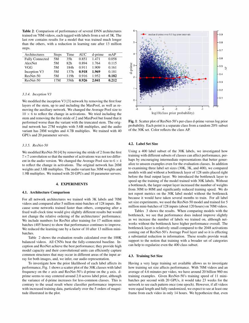
Table 2: Comparison of performance of several DNN architecturestrained on 70M videos, each tagged with labels from a set of 3K. Thelast row contains results for a model that was trained much longerthan the others, with a reduction in learning rate after 13 millionsteps.

Architectures Steps Time AUC d-prime mAPFully Connected 5M 35h 0.851 1.471 0.058AlexNet 5M 82h 0.894 1.764 0.115VGG 5M 184h 0.911 1.909 0.161Inception V3 5M 137h 0.918 1.969 0.181ResNet-50 5M 119h 0.916 1.952 0.182ResNet-50 17M 356h 0.926 2.041 0.212

3.3.4. Inception V3

We modified the inception V3 [3] network by removing the first fourlayers of the stem, up to and including the MaxPool, as well as re-moving the auxiliary network. We changed the Average Pool size to10 × 6 to reflect the change in activations. We tried including thestem and removing the first stride of 2 and MaxPool but found that itperformed worse than the variant with the truncated stem. The orig-inal network has 27M weights with 5.6B multiplies, and the audiovariant has 28M weights and 4.7B multiplies. We trained with 40GPUs and 20 parameter servers.

3.3.5. ResNet-50

We modified ResNet-50 [4] by removing the stride of 2 from the first7×7 convolution so that the number of activations was not too differ-ent in the audio version. We changed the Average Pool size to 6× 4to reflect the change in activations. The original network has 26Mweights and 3.8B multiplies. The audio variant has 30M weights and1.9B multiplies. We trained with 20 GPUs and 10 parameter servers.

4. EXPERIMENTS

4.1. Architecture Comparison

For all network architectures we trained with 3K labels and 70Mvideos and compared after 5 million mini-batches of 128 inputs. Be-cause some networks trained faster than others, comparing after afixed wall-clock time would give slightly different results but wouldnot change the relative ordering of the architectures’ performance.We include numbers for ResNet after training for 17 million mini-batches (405 hours) to show that performance continues to improve.We reduced the learning rate by a factor of 10 after 13 million mini-batches.

Table 2 shows the evaluation results calculated over the 100Kbalanced videos. All CNNs beat the fully-connected baseline. In-ception and ResNet achieve the best performance; they provide highmodel capacity and their convolutional units can efficiently capturecommon structures that may occur in different areas of the input ar-ray for both images, and, we infer, our audio representation.

To investigate how the prior likelihood of each label affects itsperformance, Fig. 1 shows a scatter plot of the 30K classes with labelfrequency on the x axis and ResNet-50’s d-prime on the y axis. d-prime seems to stay centered around 2.0 across label prior, althoughthe variance of d-prime increases for less-common classes. This iscontrary to the usual result where classifier performance improveswith increased training data, particularly over the 5 orders of magni-tude illustrated in the plot.

Fig. 1: Scatter plot of ResNet-50’s per-class d-prime versus log priorprobability. Each point is a separate class from a random 20% subsetof the 30K set. Color reflects the class AP.

4.2. Label Set Size

Using a 400 label subset of the 30K labels, we investigated howtraining with different subsets of classes can affect performance, per-haps by encouraging intermediate representations that better gener-alize to unseen examples even for the evaluation classes. In additionto examining three label set sizes (30K, 3K, and 400), we comparedmodels with and without a bottleneck layer of 128 units placed rightbefore the final output layer. We introduced the bottleneck layer tospeed up the training of the model trained with 30K labels. Withouta bottleneck, the larger output layer increased the number of weightsfrom 30M to 80M and significantly reduced training speed. We donot report metrics on the 30K label model without the bottleneckbecause it would have taken several months to train. For all labelset size experiments, we used the ResNet-50 model and trained for 5million mini-batches of 128 inputs (about 120 hours) on 70M videos.

Tables 3 shows the results. When comparing models with thebottleneck, we see that performance does indeed improve slightlyas we increase the number of labels we trained on, although net-works without the bottleneck have higher performance overall. Thebottleneck layer is relatively small compared to the 2048 activationscoming out of ResNet-50’s Average Pool layer and so it is effectinga substantial reduction in information. These results provide weaksupport to the notion that training with a broader set of categoriescan help to regularize even the 400 class subset.

4.3. Training Set Size

Having a very large training set available allows us to investigatehow training set size affects performance. With 70M videos and anaverage of 4.6 minutes per video, we have around 20 billion 960 mstraining examples. Given ResNet-50’s training speed of 11 mini-batches per second with 20 GPUs, it would take 23 weeks for thenetwork to see each pattern once (one epoch). However, if all videoswere equal length and fully randomized, we expect to see at least oneframe from each video in only 14 hours. We hypothesize that, even

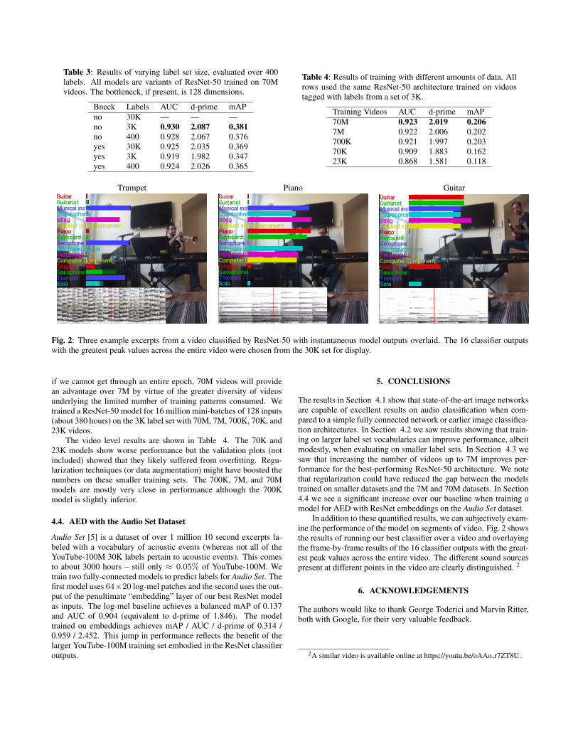
Table 3: Results of varying label set size, evaluated over 400labels. All models are variants of ResNet-50 trained on 70Mvideos. The bottleneck, if present, is 128 dimensions.

Bneck Labels AUC d-prime mAPno 30K — — —no 3K 0.930 2.087 0.381no 400 0.928 2.067 0.376yes 30K 0.925 2.035 0.369yes 3K 0.919 1.982 0.347yes 400 0.924 2.026 0.365

Table 4: Results of training with different amounts of data. Allrows used the same ResNet-50 architecture trained on videostagged with labels from a set of 3K.

Training Videos AUC d-prime mAP70M 0.923 2.019 0.2067M 0.922 2.006 0.202700K 0.921 1.997 0.20370K 0.909 1.883 0.16223K 0.868 1.581 0.118

Trumpet Piano Guitar

Fig. 2: Three example excerpts from a video classified by ResNet-50 with instantaneous model outputs overlaid. The 16 classifier outputswith the greatest peak values across the entire video were chosen from the 30K set for display.

if we cannot get through an entire epoch, 70M videos will providean advantage over 7M by virtue of the greater diversity of videosunderlying the limited number of training patterns consumed. Wetrained a ResNet-50 model for 16 million mini-batches of 128 inputs(about 380 hours) on the 3K label set with 70M, 7M, 700K, 70K, and23K videos.

The video level results are shown in Table 4. The 70K and23K models show worse performance but the validation plots (notincluded) showed that they likely suffered from overfitting. Regu-larization techniques (or data augmentation) might have boosted thenumbers on these smaller training sets. The 700K, 7M, and 70Mmodels are mostly very close in performance although the 700Kmodel is slightly inferior.

4.4. AED with the Audio Set Dataset

Audio Set [5] is a dataset of over 1 million 10 second excerpts la-beled with a vocabulary of acoustic events (whereas not all of theYouTube-100M 30K labels pertain to acoustic events). This comesto about 3000 hours – still only ≈ 0.05% of YouTube-100M. Wetrain two fully-connected models to predict labels for Audio Set. Thefirst model uses 64×20 log-mel patches and the second uses the out-put of the penultimate “embedding” layer of our best ResNet modelas inputs. The log-mel baseline achieves a balanced mAP of 0.137and AUC of 0.904 (equivalent to d-prime of 1.846). The modeltrained on embeddings achieves mAP / AUC / d-prime of 0.314 /0.959 / 2.452. This jump in performance reflects the benefit of thelarger YouTube-100M training set embodied in the ResNet classifieroutputs.

5. CONCLUSIONS

The results in Section 4.1 show that state-of-the-art image networksare capable of excellent results on audio classification when com-pared to a simple fully connected network or earlier image classifica-tion architectures. In Section 4.2 we saw results showing that train-ing on larger label set vocabularies can improve performance, albeitmodestly, when evaluating on smaller label sets. In Section 4.3 wesaw that increasing the number of videos up to 7M improves per-formance for the best-performing ResNet-50 architecture. We notethat regularization could have reduced the gap between the modelstrained on smaller datasets and the 7M and 70M datasets. In Section4.4 we see a significant increase over our baseline when training amodel for AED with ResNet embeddings on the Audio Set dataset.

In addition to these quantified results, we can subjectively exam-ine the performance of the model on segments of video. Fig. 2 showsthe results of running our best classifier over a video and overlayingthe frame-by-frame results of the 16 classifier outputs with the great-est peak values across the entire video. The different sound sourcespresent at different points in the video are clearly distinguished. 2

6. ACKNOWLEDGEMENTS

The authors would like to thank George Toderici and Marvin Ritter,both with Google, for their very valuable feedback.

2A similar video is available online at https://youtu.be/oAAo r7ZT8U.

7. REFERENCES

[1] A. Krizhevsky, I. Sutskever, and G. E. Hinton, “Imagenet clas-sification with deep convolutional neural networks,” in Ad-vances in neural information processing systems, 2012, pp.1097–1105.

[2] K. Simonyan and A. Zisserman, “Very deep convolutionalnetworks for large-scale image recognition,” arXiv preprintarXiv:1409.1556, 2014.

[3] C. Szegedy, V. Vanhoucke, S. Ioffe, J. Shlens, and Z. Wojna,“Rethinking the inception architecture for computer vision,”arXiv preprint arXiv:1512.00567, 2015.

[4] K. He, X. Zhang, S. Ren, and J. Sun, “Deep residual learn-ing for image recognition,” arXiv preprint arXiv:1512.03385,2015.

[5] J. F. Gemmeke, D. P. W. Ellis, D. Freedman, A. Jansen,W. Lawrence, R. C. Moore, M. Plakal, and M. Ritter, “Au-dio Set: An ontology and human-labeled dartaset for audioevents,” in IEEE ICASSP 2017, New Orleans, 2017.

[6] J. Deng, W. Dong, R. Socher, L.-J. Li, K. Li, and L. Fei-Fei, “Imagenet: A large-scale hierarchical image database,” inComputer Vision and Pattern Recognition, 2009. CVPR 2009.IEEE Conference on. IEEE, 2009, pp. 248–255.

[7] R. F. Lyon, “Machine hearing: An emerging field [exploratorydsp],” Ieee signal processing magazine, vol. 27, no. 5, pp. 131–139, 2010.

[8] A. Mesaros, T. Heittola, A. Eronen, and T. Virtanen, “Acousticevent detection in real life recordings,” in Signal ProcessingConference, 2010 18th European. IEEE, 2010, pp. 1267–1271.

[9] X. Zhuang, X. Zhou, M. A. Hasegawa-Johnson, and T. S.Huang, “Real-world acoustic event detection,” Pattern Recog-nition Letters, vol. 31, no. 12, pp. 1543–1551, 2010.

[10] J. F. Gemmeke, L. Vuegen, P. Karsmakers, B. Vanrumste, et al.,“An exemplar-based nmf approach to audio event detection,” in2013 IEEE Workshop on Applications of Signal Processing toAudio and Acoustics. IEEE, 2013, pp. 1–4.

[11] A. Temko, R. Malkin, C. Zieger, D. Macho, C. Nadeu, andM. Omologo, “Clear evaluation of acoustic event detectionand classification systems,” in International Evaluation Work-shop on Classification of Events, Activities and Relationships.Springer, 2006, pp. 311–322.

[12] N. Takahashi, M. Gygli, B. Pfister, and L. Van Gool, “Deepconvolutional neural networks and data augmentation foracoustic event detection,” arXiv preprint arXiv:1604.07160,2016.

[13] G. Parascandolo, H. Huttunen, and T. Virtanen, “Recurrentneural networks for polyphonic sound event detection in reallife recordings,” in 2016 IEEE International Conference onAcoustics, Speech and Signal Processing (ICASSP). IEEE,2016, pp. 6440–6444.

[14] G. Awad, J. Fiscus, M. Michel, D. Joy, W. Kraaij, A. F.Smeaton, G. Quenot, M. Eskevich, R. Aly, and R. Ordelman,“Trecvid 2016: Evaluating video search, video event detection,localization, and hyperlinking,” in Proceedings of TRECVID2016. NIST, USA, 2016.

[15] B. G. Fabian Caba Heilbron, Victor Escorcia and J. C. Niebles,“Activitynet: A large-scale video benchmark for human activ-ity understanding,” in Proceedings of the IEEE Conference onComputer Vision and Pattern Recognition, 2015, pp. 961–970.

[16] A. Karpathy, G. Toderici, S. Shetty, T. Leung, R. Sukthankar,and L. Fei-Fei, “Large-scale video classification with convolu-tional neural networks,” in CVPR, 2014.

[17] A. Mesaros, T. Heittola, and T. Virtanen, “TUT database foracoustic scene classification and sound event detection,” in24th European Signal Processing Conference 2016 (EUSIPCO2016), Budapest, Hungary, 2016, http://www.cs.tut.fi/sgn/arg/dcase2016/.

[18] T. N. Sainath, O. Vinyals, A. Senior, and H. Sak, “Convolu-tional, long short-term memory, fully connected deep neuralnetworks,” in 2015 IEEE International Conference on Acous-tics, Speech and Signal Processing (ICASSP). IEEE, 2015, pp.4580–4584.

[19] H. Eghbal-Zadeh, B. Lehner, M. Dorfer, and G. Widmer, “Cp-jku submissions for dcase-2016: A hybrid approach using bin-aural i-vectors and deep convolutional neural networks,” .

[20] J. Yue-Hei Ng, M. Hausknecht, S. Vijayanarasimhan,O. Vinyals, R. Monga, and G. Toderici, “Beyond short snip-pets: Deep networks for video classification,” in Proceed-ings of the IEEE Conference on Computer Vision and PatternRecognition, 2015, pp. 4694–4702.

[21] A. Kumar and B. Raj, “Audio event detection using weaklylabeled data,” arXiv preprint arXiv:1605.02401, 2016.

[22] A. Singhal, “Introducing the knowledge graph:things, not strings,” 2012, Official Google blog,https://googleblog.blogspot.com/2012/05/introducing-knowledge-graph-things-not.html.

[23] M. Abadi et al., “TensorFlow: Large-scale machine learningon heterogeneous systems,” 2015, Software available from ten-sorflow.org.

[24] D. Kingma and J. Ba, “Adam: A method for stochastic opti-mization,” arXiv preprint arXiv:1412.6980, 2014.

[25] S. Ioffe and C. Szegedy, “Batch normalization: Accelerat-ing deep network training by reducing internal covariate shift,”arXiv preprint arXiv:1502.03167, 2015.

[26] N. Srivastava, G. E. Hinton, A. Krizhevsky, I. Sutskever, andR. Salakhutdinov, “Dropout: a simple way to prevent neuralnetworks from overfitting.,” Journal of Machine Learning Re-search, vol. 15, no. 1, pp. 1929–1958, 2014.

[27] T. Fawcett, “Roc graphs: Notes and practical considerationsfor researchers,” Machine learning, vol. 31, no. 1, pp. 1–38,2004.

[28] C. Buckley and E. M. Voorhees, “Retrieval evaluation withincomplete information,” in Proceedings of the 27th annualinternational ACM SIGIR conference on Research and devel-opment in information retrieval. ACM, 2004, pp. 25–32.

[29] V. Nair and G. E. Hinton, “Rectified linear units improve re-stricted boltzmann machines,” in Proceedings of the 27th Inter-national Conference on Machine Learning (ICML-10), 2010,pp. 807–814.