Embed Size (px)
Citation preview
8/14/2019 Shock-Wave Heating Model for Chondrule Formation
http://slidepdf.com/reader/full/shock-wave-heating-model-for-chondrule-formation 1/50
a r X i v : a s
t r o - p h / 0 6 1 1 2 8 9 v 1
9 N o v 2 0 0 6
Accepted in Icarus, November 4, 2006
Shock-Wave Heating Model for Chondrule Formation:
Hydrodynamic Simulation of Molten Droplets exposed to Gas Flows
Hitoshi Miura,a,1,∗ Taishi Nakamotob,c
aDepartment of Physics, Kyoto University, Kitashirakawa, Sakyo, Kyoto 606-8502,
Japan∗Corresponding Author E-mail address: [email protected]
bCenter for Computational Sciences, University of Tsukuba, Tsukuba, Ibaraki
305-8577, JapancPresent Address: Department of Earth and Planetary Sciences, Tokyo Institute of
Technology, Meguro, Tokyo 152-8551, Japan
1Research Fellow of the Japan Society for the Promotion of Science
Pages: 50
Tables: 1
Figures: 13
1
8/14/2019 Shock-Wave Heating Model for Chondrule Formation
http://slidepdf.com/reader/full/shock-wave-heating-model-for-chondrule-formation 2/50
Proposed Running Head: Hydrodynamics of Molten Droplets in Gas Flow
Editorial correspondence to:
Dr. Hitoshi Miura
Theoretical Astrophysics Group, Department of Physics, Kyoto University
Kitashirakawa, Sakyo, Kyoto 606-8502, Japan
Phone: +81-75-753-3880
Fax: +81-75-753-3886
E-mail: [email protected]
2
8/14/2019 Shock-Wave Heating Model for Chondrule Formation
http://slidepdf.com/reader/full/shock-wave-heating-model-for-chondrule-formation 3/50
Abstract
Millimeter-sized, spherical silicate grains abundant in chondritic me-teorites, which are called as chondrules, are considered to be a strong
evidence of the melting event of the dust particles in the protoplanetary
disk. One of the most plausible scenarios is that the chondrule precursor
dust particles are heated and melt in the high-velocity gas flow (shock-
wave heating model). We developed the non-linear, time-dependent, and
three-dimensional hydrodynamic simulation code for analyzing the dy-
namics of molten droplets exposed to the gas flow. We confirmed that
our simulation results showed a good agreement in a linear regime with
the linear solution analytically derived by Sekiya et al. (2003). We found
that the non-linear terms in the hydrodynamical equations neglected by
Sekiya et al. (2003) can cause the cavitation by producing negative pres-
sure in the droplets. We discussed that the fragmentation through thecavitation is a new mechanism to determine the upper limit of chondrule
sizes. We also succeeded to reproduce the fragmentation of droplets when
the gas ram pressure is stronger than the effect of the surface tension. Fi-
nally, we compared the deformation of droplets in the shock-wave heating
with the measured data of chondrules and suggested the importance of
other effects to deform droplets, for example, the rotation of droplets. We
believe that our new code is a very powerful tool to investigate the hydro-
dynamics of molten droplets in the framework of the shock-wave heating
model and has many potentials to be applied to various problems.
Keywords: meteorites, Solar System origin, Solar Nebula
3
8/14/2019 Shock-Wave Heating Model for Chondrule Formation
http://slidepdf.com/reader/full/shock-wave-heating-model-for-chondrule-formation 4/50
1 Introduction
Chondrules are millimeter-sized, once-molten, spherical-shaped grains mainlycomposed of silicate material. They are abundant in chondritic mete-
orites, which are the majority of meteorites falling onto the Earth. They
are considered to have formed from chondrule precursor dust particles
about 4.56 × 10⁹ yr ago in the solar nebula (Amelin et al. 2002); they
were heated and melted through flash heating events in the solar nebula
and cooled again to solidify in a short period of time (e.g., Jones et al.
2000 and references therein). So they must have great information on the
early history of our solar system. Since it is naturally expected that pro-
toplanetary disks around young stars in star forming regions have similar
dust particles and processes, the study of chondrule formation may pro-
vide us much information on the planetary system formation. Chondrules
have many features: physical properties (sizes, shapes, densities, degree of
magnetization, etc.), isotopic compositions (oxygen, nitrogen, rare gases,
etc.), mineralogical and petrologic features (structures, crystals, degrees
of alteration, relicts, etc.), and so forth, each of which should be a clue
that helps us to reveal their own formation process and that of the plan-
etary system. To reveal their formation history, many works have b een
carried out observationally, experimentally, and theoretically.
Shock-wave heating model is considered to be one of the most plausible
models for chondrule formation (Boss 1996, Jones et al. 2000). This model
has been investigated theoretically by many authors (Hood & Horanyi
1991, 1993, Ruzmaikina & Ip 1994, Tanaka et al. 1998, Hood 1998, Iida et
al. 2001, Desch & Connolly 2002, Miura et al. 2002, Ciesla & Hood 2002,Miura & Nakamoto 2005, 2006). One of the special features of this model
is that chondrule precursor dust particles are exposed to the high-velocity
rarefied gas flow. In the gas flow, the gas frictional heating takes place to
heat and melt the precursor dust particles (the condition to melt silicate
dust particles was derived by Iida et al. 2001). Therefore, it is naturally
thought that the ram pressure of the gas flow affects the molten dust
particles. Susa & Nakamoto (2002) estimated the maximum radius of the
molten droplet above which the droplet should be destroyed by the ram
pressure. They analyzed the non-linear phenomena like a fragmentation
by an order of magnitude estimation. On the contrary, Sekiya et al.
(2003) derived a linear solution of the deformation and the internal flow
of the molten droplet exposed to the rarefied gas flow. They analytically
solved the hydrodynamical equations assuming that the non-linear terms
of the hydrodynamical equations as well as the surface deformation are
sufficiently small so that linearized equations are appropriate.
The hydrodynamics of the molten droplet exposed to the rarefied gas
4
8/14/2019 Shock-Wave Heating Model for Chondrule Formation
http://slidepdf.com/reader/full/shock-wave-heating-model-for-chondrule-formation 5/50
flow is an important aspect of the shock-wave heating model. The inter-
nal flow causes the homogenization of the chemical/isotopic compositions
and temperature distribution in the molten precursor dust particles. The
deformation of the molten droplet might result into the deformed chon-
drules. Moreover, the fragmentation of the molten droplet gives an upper
limit of chondrules as pointed by Susa & Nakamoto (2002). However,
the analysis of Susa & Nakamoto (2002) did not take into account the
hydrodynamics of the droplet and the formulation of Sekiya et al. (2003)
cannot be applied to such non-linear phenomena like the fragmentation.
Additionally, the effects of non-linear terms in the hydrodynamical equa-
tions, which was neglected in Sekiya et al. (2003), might be important in
the hydrodynamics. In order to solve the hydrodynamical equations in-
cluding the non-linear terms, the numerical simulations can be a powerful
tool. The purpose of this study is to develop a numerical model of themolten droplet exposed to the high-velocity rarefied gas flow.
We describe the physical model in §2 and the basic equations in §3.
The numerical model is summarized in §4. We show the calculation results
in §5 and some discussions in §6. Finally, we make conclusions in §7. Some
numerical techniques we use in our model are summarized in appendixes.
2 Physical Model
We are considering the molten silicate dust particles exposed to the high-
velocity rarefied gas flow. These dust particles are, of course, initially
solid and then melted due to the gas frictional heating. In this paper, we
do not consider how the solid particles melt in the gas flow. We assume
the completely molten droplets (no solid lumps inside) and the physical
properties of the droplet (the coefficient of viscosity and the fluid surface
tension coefficient) are constant. The droplet behaves as an incompressible
fluid because the sound speed (∼ a few km s−1, Murase & McBirney 1973)
is much larger than the fluid velocity expected in the droplet (∼ a few
tens cms−1, Sekiya et al. 2003).
The ram pressure of the gas flow is acting on the droplet surface ex-
posed to the high-velocity gas flow. It should be noted that the gas flow
we consider here does not follow the hydrodynamical equations in the spa-
tial scale of chondrules because the nebular gas is too rarefied. The mean
free path of the nebula gas can be estimated by l = 1/(ns), where s isthe collisional cross section of gas molecules and n is the number density
of the nebular gas. In the minimum mass solar nebula model (Hayashi et
al. 1985), the number density of the nebula gas at 1 AU from the central
star is about n ≃ 1014 cm−3. The collisional cross section of the hydro-
5
8/14/2019 Shock-Wave Heating Model for Chondrule Formation
http://slidepdf.com/reader/full/shock-wave-heating-model-for-chondrule-formation 6/50
gen molecule is roughly estimated as s ≃ 10−16 cm2 (e.g., Hollenbach &
McKee 1979). So, we obtain l
≃100 cm. On the contrary, the typical size
of chondrules is about a few 100 µm (e.g., Rubin & Keil 1984). Namely,
the object which disturbs the gas flow is much smaller than the mean free
path of the gas. This condition corresponds to a free molecular flow in
which gas molecules scattered and reemitted from the droplet surface do
not disturb the free stream velocity distribution. Therefore, in our model,
the ram pressure acting on the droplet surface per unit area is explicitly
given by the momentum flux of the molecular gas flow pfm = ρgv2rel, where
ρg is the nebula gas density and vrel is the relative velocity between the gas
and the mass center of the droplet. This force causes the deceleration of
the center of mass. In the coordinate system co-moving with the center of
mass (we adopt this coordinate in our model), the apparent gravitational
acceleration should be considered.Strictly speaking, the relative velocity of a gas molecule and a surface
fluid element is not vrel, since the latter has a non-zero velocity in the
rest frame of the mass center of the droplet. However, the liquid velocity
is much smaller than the gas molecular velocity, and is negligible (Sekiya
et al. 2003). In hypersonic free molecular flow, the thermal and reflected
velocities of gas molecules are also sufficiently small and are ignored.
3 Basic Equations
3.1 Equation of Continuity
Generally, Eulerian methods like the CIP scheme (e.g., Yabe et al. 2001)
use a color function φ in the multi-phase analysis. For example, when a
fluid of phase k occupies a certain region, the color function takes φk = 1
inside the region and φk = 0 outside. In this paper, we define φ = 1 for
inside the molten dust particle and φ = 0 for outside (ambient region).
Using the color function, the density of the fluid element ρ is given by
ρ = ρd × φ + ρa × (1 − φ), (1)
where the subscripts “d” and “a” indicate the inherent values for the
molten silicate dust particle (droplet) and the ambient region, respectively.
The other physical values of the fluid element (the coefficient of viscosity
µ and the sound speed cs) are given in the same manner, namely, µ =
µd × φ + µa × (1− φ) and cs = cs,d × φ + cs,a × (1− φ), respectively1.
1In the numerical simulation, an undesirable situation that the hydrostatic pressure p
becomes much larger than the value of the ambient region in spite of φ ≪ 1 could occur.
When it occurred, we set the sound speed of the fluid element cs → cs,d in order to avoid the
difficulty in the numerical simulation.
6
8/14/2019 Shock-Wave Heating Model for Chondrule Formation
http://slidepdf.com/reader/full/shock-wave-heating-model-for-chondrule-formation 7/50
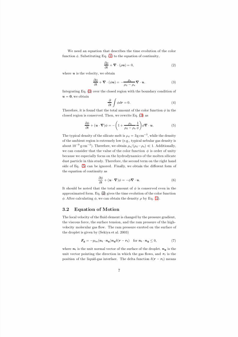
We need an equation that describes the time evolution of the color
function φ. Substituting Eq. (1) to the equation of continuity,
∂ρ
∂t+∇ · (ρu) = 0, (2)
where u is the velocity, we obtain
∂φ
∂t+∇ · (φu) = − ρa
ρd − ρa∇ · u. (3)
Integrating Eq. (3) over the closed region with the boundary condition of
u = 0, we obtain∂
∂t
φdr = 0. (4)
Therefore, it is found that the total amount of the color function φ in the
closed region is conserved. Then, we rewrite Eq. ( 3) as
∂φ
∂t+ (u ·∇)φ = −
1 +
ρa
ρd − ρa
1
φ
φ∇ · u. (5)
The typical density of the silicate melt is ρd = 3 g cm−3, while the density
of the ambient region is extremely low (e.g., typical nebular gas density is
about 10−9 g cm−3). Therefore, we obtain ρa/(ρd−ρa) ≪ 1. Additionally,
we can consider that the value of the color function φ is order of unity
because we especially focus on the hydrodynamics of the molten silicate
dust particle in this study. Therefore, the second term on the right hand
side of Eq. (5) can be ignored. Finally, we obtain the different form of
the equation of continuity as
∂φ∂t
+ (u ·∇)φ = −φ∇ · u. (6)
It should be noted that the total amount of φ is conserved even in the
approximated form. Eq. (6) gives the time evolution of the color function
φ. After calculating φ, we can obtain the density ρ by Eq. (1).
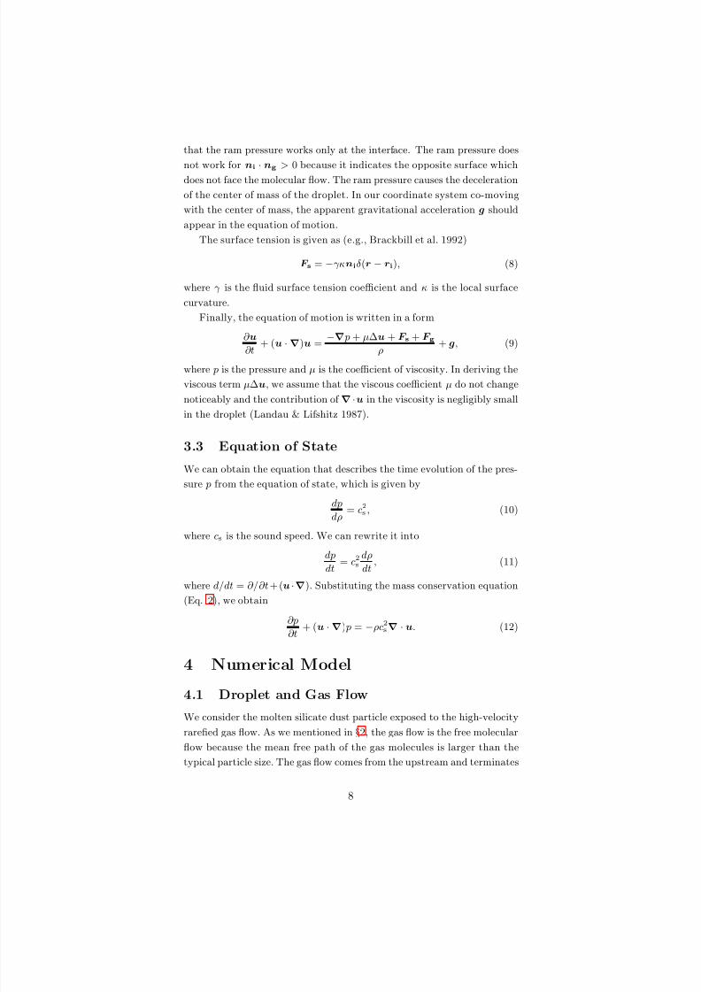
3.2 Equation of Motion
The local velocity of the fluid element is changed by the pressure gradient,
the viscous force, the surface tension, and the ram pressure of the high-
velocity molecular gas flow. The ram pressure exerted on the surface of
the droplet is given by (Sekiya et al. 2003)
F g = − pfm(ni · ng)ngδ(r − ri) for ni · ng ≤ 0, (7)
where ni is the unit normal vector of the surface of the droplet, ng is the
unit vector pointing the direction in which the gas flows, and ri is the
position of the liquid-gas interface. The delta function δ(r − ri) means
7
8/14/2019 Shock-Wave Heating Model for Chondrule Formation
http://slidepdf.com/reader/full/shock-wave-heating-model-for-chondrule-formation 8/50
that the ram pressure works only at the interface. The ram pressure does
not work for ni
·ng > 0 because it indicates the opposite surface which
does not face the molecular flow. The ram pressure causes the deceleration
of the center of mass of the droplet. In our coordinate system co-moving
with the center of mass, the apparent gravitational acceleration g should
appear in the equation of motion.
The surface tension is given as (e.g., Brackbill et al. 1992)
F s = −γκniδ(r − ri), (8)
where γ is the fluid surface tension coefficient and κ is the local surface
curvature.
Finally, the equation of motion is written in a form
∂ u
∂t + (u ·∇
)u = −∇ p + µ∆u + F s + F g
ρ + g, (9)
where p is the pressure and µ is the coefficient of viscosity. In deriving the
viscous term µ∆u, we assume that the viscous coefficient µ do not change
noticeably and the contribution of ∇ ·u in the viscosity is negligibly small
in the droplet (Landau & Lifshitz 1987).
3.3 Equation of State
We can obtain the equation that describes the time evolution of the pres-
sure p from the equation of state, which is given by
dp
dρ
= c2s , (10)
where cs is the sound speed. We can rewrite it into
dp
dt= c2s
dρ
dt, (11)
where d/dt = ∂/∂t +(u ·∇). Substituting the mass conservation equation
(Eq. 2), we obtain
∂p
∂t+ (u ·∇) p = −ρc2s∇ · u. (12)
4 Numerical Model
4.1 Droplet and Gas Flow
We consider the molten silicate dust particle exposed to the high-velocity
rarefied gas flow. As we mentioned in §2, the gas flow is the free molecular
flow because the mean free path of the gas molecules is larger than the
typical particle size. The gas flow comes from the upstream and terminates
8
8/14/2019 Shock-Wave Heating Model for Chondrule Formation
http://slidepdf.com/reader/full/shock-wave-heating-model-for-chondrule-formation 9/50
when it collide with the dust surface. Figure 1 shows the schematic picture
of our numerical model and the coordinate system. The black thick arrows
show the stream line of the gas flow. The gas flow gives the momentum
to the dust particle at the area where it terminates. Therefore, the ram
pressure exerted on the dust surface F g can be calculated easily, even if
we do not solve the hydrodynamic equations for the ambient region. The
numerical treatment of the ram pressure is described in §A.2.2.
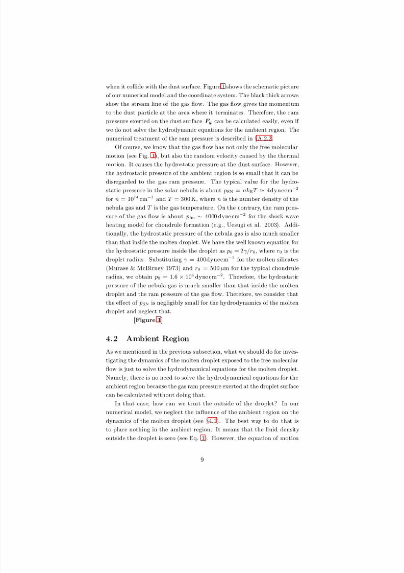
Of course, we know that the gas flow has not only the free molecular
motion (see Fig. 1), but also the random velocity caused by the thermal
motion. It causes the hydrostatic pressure at the dust surface. However,
the hydrostatic pressure of the ambient region is so small that it can be
disregarded to the gas ram pressure. The typical value for the hydro-
static pressure in the solar nebula is about pSN = nkBT ≃ 4dynecm−2
for n = 1014
cm−3
and T = 300 K, where n is the number density of thenebula gas and T is the gas temperature. On the contrary, the ram pres-
sure of the gas flow is about pfm ∼ 4000 dyne cm−2 for the shock-wave
heating model for chondrule formation (e.g., Uesugi et al. 2003). Addi-
tionally, the hydrostatic pressure of the nebula gas is also much smaller
than that inside the molten droplet. We have the well known equation for
the hydrostatic pressure inside the droplet as p0 = 2γ/r0, where r0 is the
droplet radius. Substituting γ = 400dynecm−1 for the molten silicates
(Murase & McBirney 1973) and r0 = 500 µm for the typical chondrule
radius, we obtain p0 = 1.6 × 10⁴ dyne cm−2. Therefore, the hydrostatic
pressure of the nebula gas is much smaller than that inside the molten
droplet and the ram pressure of the gas flow. Therefore, we consider that
the effect of pSN is negligibly small for the hydrodynamics of the molten
droplet and neglect that.
[Figure 1]
4.2 Ambient Region
As we mentioned in the previous subsection, what we should do for inves-
tigating the dynamics of the molten droplet exposed to the free molecular
flow is just to solve the hydrodynamical equations for the molten droplet.
Namely, there is no need to solve the hydrodynamical equations for the
ambient region because the gas ram pressure exerted at the droplet surface
can be calculated without doing that.
In that case, how can we treat the outside of the droplet? In our
numerical model, we neglect the influence of the ambient region on the
dynamics of the molten droplet (see §4.1). The best way to do that is
to place nothing in the ambient region. It means that the fluid density
outside the droplet is zero (see Eq. 1). However, the equation of motion
9
8/14/2019 Shock-Wave Heating Model for Chondrule Formation
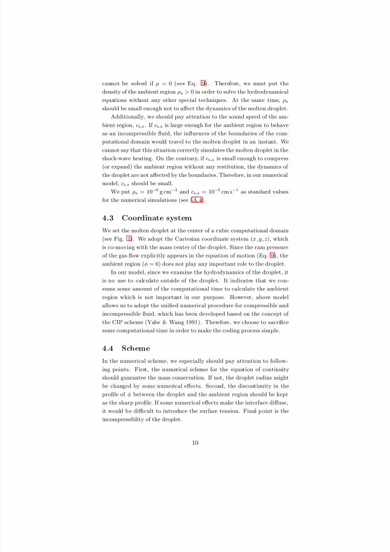
http://slidepdf.com/reader/full/shock-wave-heating-model-for-chondrule-formation 10/50
cannot be solved if ρ = 0 (see Eq. 9). Therefore, we must put the
density of the ambient region ρa > 0 in order to solve the hydrodynamical
equations without any other special techniques. At the same time, ρa
should be small enough not to affect the dynamics of the molten droplet.
Additionally, we should pay attention to the sound speed of the am-
bient region, cs,a. If cs,a is large enough for the ambient region to behave
as an incompressible fluid, the influences of the boundaries of the com-
putational domain would travel to the molten droplet in an instant. We
cannot say that this situation correctly simulates the molten droplet in the
shock-wave heating. On the contrary, if cs,a is small enough to compress
(or expand) the ambient region without any restitution, the dynamics of
the droplet are not affected by the boundaries. Therefore, in our numerical
model, cs,a should be small.
We put ρa = 10−6
g cm−3
and cs,a = 10−5
cm s−1
as standard valuesfor the numerical simulations (see §A.4).
4.3 Coordinate system
We set the molten droplet at the center of a cubic computational domain
(see Fig. 1). We adopt the Cartesian coordinate system (x,y,z), which
is co-moving with the mass center of the droplet. Since the ram pressure
of the gas flow explicitly appears in the equation of motion (Eq. 9), the
ambient region (φ = 0) does not play any important role to the droplet.
In our model, since we examine the hydrodynamics of the droplet, it
is no use to calculate outside of the droplet. It indicates that we con-
sume some amount of the computational time to calculate the ambientregion which is not important in our purpose. However, above model
allows us to adopt the unified numerical procedure for compressible and
incompressible fluid, which has been developed based on the concept of
the CIP scheme (Yabe & Wang 1991). Therefore, we choose to sacrifice
some computational time in order to make the coding process simple.
4.4 Scheme
In the numerical scheme, we especially should pay attention to follow-
ing points. First, the numerical scheme for the equation of continuity
should guarantee the mass conservation. If not, the droplet radius might
be changed by some numerical effects. Second, the discontinuity in theprofile of φ between the droplet and the ambient region should be kept
as the sharp profile. If some numerical effects make the interface diffuse,
it would b e difficult to introduce the surface tension. Final p oint is the
incompressiblity of the droplet.
10
8/14/2019 Shock-Wave Heating Model for Chondrule Formation
http://slidepdf.com/reader/full/shock-wave-heating-model-for-chondrule-formation 11/50
The equation of continuity in the form of Eq. (6) can be rewritten as
∂φ∂t +∇ · (φu) = 0, (13)
where the total amount of φ in a closed region should be conserved. The
R-CIP-CSL2 scheme is one of the recent versions of the CIP scheme,
which guarantees the exact conservation even in the framework of a semi-
Lagrangian scheme (Nakamura et al. 2001). In order to solve Eq. (13),
we adopt the R-CIP-CSL2 scheme and briefly describe this scheme in
appendix A.1.2. Additionally, we make a proper correction for the velocity
u before solving Eq. (13) in order to keep the incompressibility of the
droplet (see appendix A.3).
The other two hydrodynamical equations can be separated into the
advection phase and the non-advection phase. The advection phases of
the equation of motion (Eq. 9) and the equation of state (Eq. 12) arewritten as
∂ u
∂t+ (u ·∇)u = 0,
∂p
∂t+ (u ·∇) p = 0. (14)
We solve above equations using the R-CIP scheme, which is the oscillation
preventing scheme for advection equation (Xiao et al. 1996b, see appendix
A.1.1). The non-advection phases can be written as
∂ u
∂t= −∇ p
ρ+Q
ρ,
∂p
∂t= −ρc2s∇ · u, (15)
where Q is the summation of forces except for the pressure gradient.
The problem intrinsic in incompressible fluid is in the high sound speed
in the pressure equation. Yabe & Wang (1991) introduced an excellent
approach to avoid the problem (see appendix A.2.1). It is called as theC-CUP scheme (Yabe et al. 2001).
Additionally, we introduce the anti-diffusion technique when calculat-
ing the equation of continuity by the R-CIP-CSL2 scheme. The original
R-CIP-CSL2 scheme provides an excellent solution for the conservative
equation (e.g., Nakamura et al. 2001). However, if the initial profile
of φ has a sharp discontinuity (e.g., rectangle wave), the profile is los-
ing its sharpness as the time step progresses. It is a result of the nu-
merical diffusion. In order to keep the discontinuity of the profile, the
anti-diffusion modification is an useful technique (e.g., Xiao & Ikebata
2003). In this paper, we explicitly add the diffusion term with a negative
diffusion coefficient to the CIP-CSL2 scheme (see appendix A.1.3). We
perform the one-dimensional conservative equation with or without the
anti-diffusion technique in order to show the validity of this method (see
appendix A.1.4).
For the multi-dimensions, we use a directional splitting technique to
perform sequential one-dimensional procedure in each direction. We adopt
11
8/14/2019 Shock-Wave Heating Model for Chondrule Formation
http://slidepdf.com/reader/full/shock-wave-heating-model-for-chondrule-formation 12/50
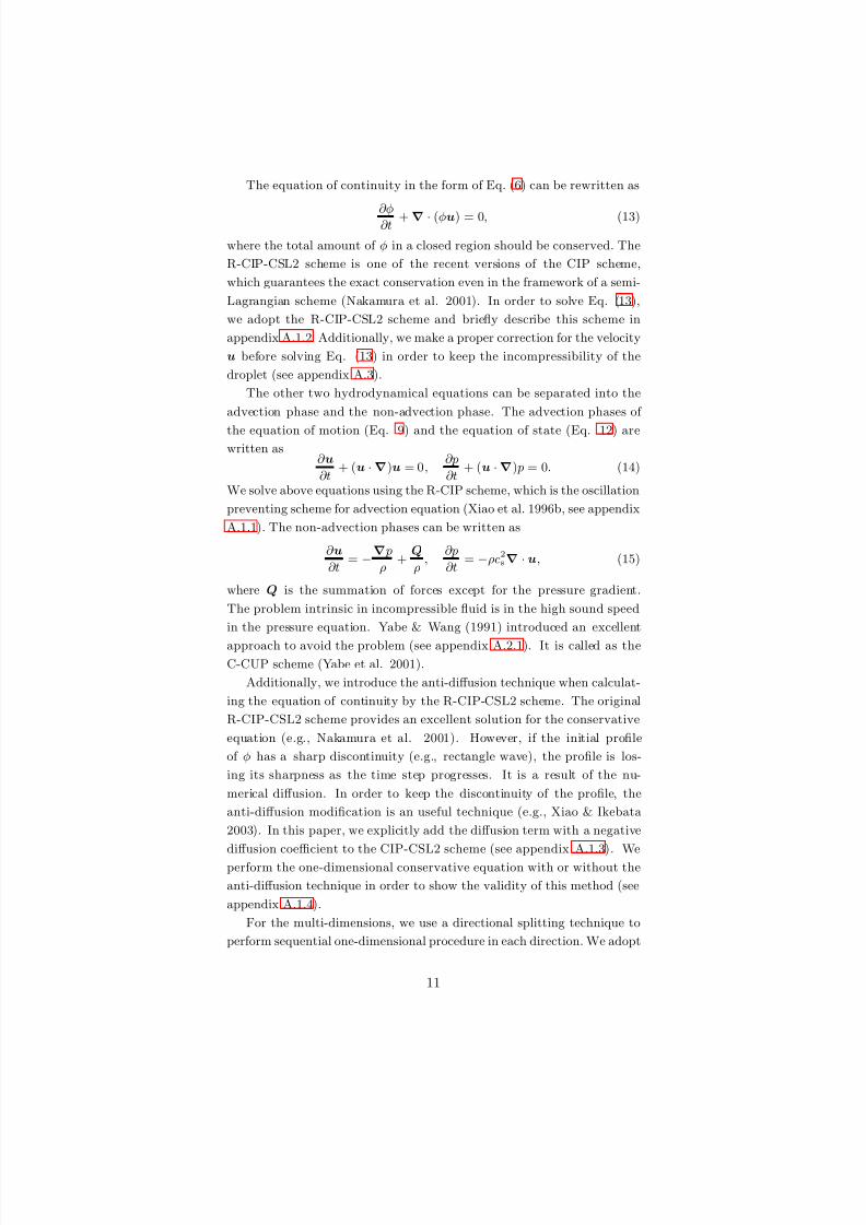
the staggered grid for digitizing the physical variables in the hydrody-
namical equations (see Fig. 2). The scalar variables are defined at the
cell-center and the velocity u = (u,v,w) is defined on the cell-edge. The
surface tension and the ram pressure are defined at the cell-center. The
numerical model of these two forces are shown in appendixes A.2.2 and
A.2.3. When calculating these two forces, the gradient field of φ is re-
quired and needs to be artificially smoothed (e.g., Yabe et al. 2001, see
appendix A.2.4 in this paper). Note that the smoothing is done only
at the calculation of these two forces and the original profile with sharp
discontinuity is unchanged.
[Figure 2]
5 Results
5.1 Input Parameters and Initial Settings
We investigate various cases about the droplet radius, r0 = 100, 200,
500, 1000, 2000, 5000 µm, 1 cm, and 2 cm. The momentum flux of the
gas flow is set as pfm = 4000 dyne cm−2, which may be realized in the
shock-wave heating model for relatively high-density shock waves (Uesugi
et al. 2003). The coefficient of viscosity of silicate melts µd strongly
depends on the temperature and the chemical composition. We adopt
µd = 1.3 g c m−1 s−1 from the model of Uesugi et al. (2003), in which they
calculated the viscosity by the formulation of Bottinga & Weill (1972)
assuming the temperature
∼1800 K and the chemical composition of BO
type chondrule. The surface tension γ = 400dynecm−1 and the sound
speed of the molten droplet cs,d = 2 × 105 cm s−1 are the typical value
of the silicate melts (Murase & McBirney 1973). Other input parameters
are listed in Table 1. When we consider the fragmentation process of
the droplets in the gas flow, it is useful to introduce the non-dimensional
parameter W e ≡ pfmr0/γ , which is called as the Weber number and indi-
cates the ratio of the ram pressure of the gas flow to the surface tension
of the droplet. Some experiments suggested that the droplets fragment
for W e ∼ 6 − 22 or higher (Bronshten 1983).
[Table 1]
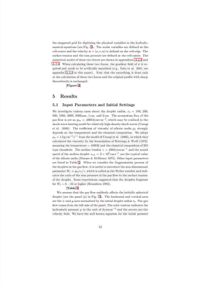
We assume that the gas flow suddenly affects the initially spherical
droplet (see the panel (a) in Fig. 3). The horizontal and vertical axes
are the x- and y-axes normalized by the initial droplet radius r0. The gas
flow comes from the left side of the panel. The color contour indicates the
hydrostatic pressure p in the unit of dynecm−2 and the arrows are the
velocity field. We have the well known equation for the initial pressure
12
8/14/2019 Shock-Wave Heating Model for Chondrule Formation
http://slidepdf.com/reader/full/shock-wave-heating-model-for-chondrule-formation 13/50
inside the droplet as p = 2γ/r0 and p = 0 for outside. The red curves
indicate the contour of the color function φ after smoothing. Thick solid
curve indicates φ = 0.5, which means the interface between the droplet
and the ambient region, and the dashed and the dotted-dashed curves are
φ = 0.1 and 0.9, which are drawn in order to show the effective width of
the transition region between the molten droplet and the ambient region.
The initial internal velocity of the droplet is set to be all zero. The
computational grid points are set to be 60 × 60 × 60 for the standard
calculations. The boundary conditions are u = 0, p = 0, ρ = ρa, φ = 0,
and σ = 0.
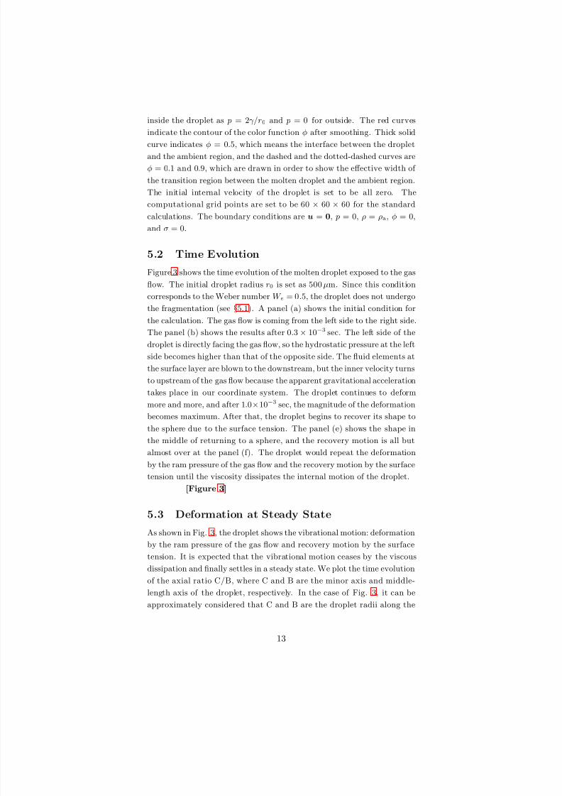
5.2 Time Evolution
Figure 3 shows the time evolution of the molten droplet exposed to the gas
flow. The initial droplet radius r0 is set as 500 µm. Since this condition
corresponds to the Weber number W e = 0.5, the droplet does not undergo
the fragmentation (see §5.1). A panel (a) shows the initial condition for
the calculation. The gas flow is coming from the left side to the right side.
The panel (b) shows the results after 0.3 × 10⁻³ sec. The left side of the
droplet is directly facing the gas flow, so the hydrostatic pressure at the left
side becomes higher than that of the opposite side. The fluid elements at
the surface layer are blown to the downstream, but the inner velocity turns
to upstream of the gas flow because the apparent gravitational acceleration
takes place in our coordinate system. The droplet continues to deform
more and more, and after 1.0×10⁻³ sec, the magnitude of the deformation
becomes maximum. After that, the droplet begins to recover its shape tothe sphere due to the surface tension. The panel (e) shows the shape in
the middle of returning to a sphere, and the recovery motion is all but
almost over at the panel (f). The droplet would repeat the deformation
by the ram pressure of the gas flow and the recovery motion by the surface
tension until the viscosity dissipates the internal motion of the droplet.
[Figure 3]
5.3 Deformation at Steady State
As shown in Fig. 3, the droplet shows the vibrational motion: deformation
by the ram pressure of the gas flow and recovery motion by the surface
tension. It is expected that the vibrational motion ceases by the viscousdissipation and finally settles in a steady state. We plot the time evolution
of the axial ratio C/B, where C and B are the minor axis and middle-
length axis of the droplet, respectively. In the case of Fig. 3, it can be
approximately considered that C and B are the droplet radii along the
13
8/14/2019 Shock-Wave Heating Model for Chondrule Formation
http://slidepdf.com/reader/full/shock-wave-heating-model-for-chondrule-formation 14/50
x- and y-axes, respectively (see §6.3). Therefore, C/B is an indicator of
the droplet deformation, for example, C/B = 1 approximately indicates a
sphere and smaller C/B indicates a larger deformation.
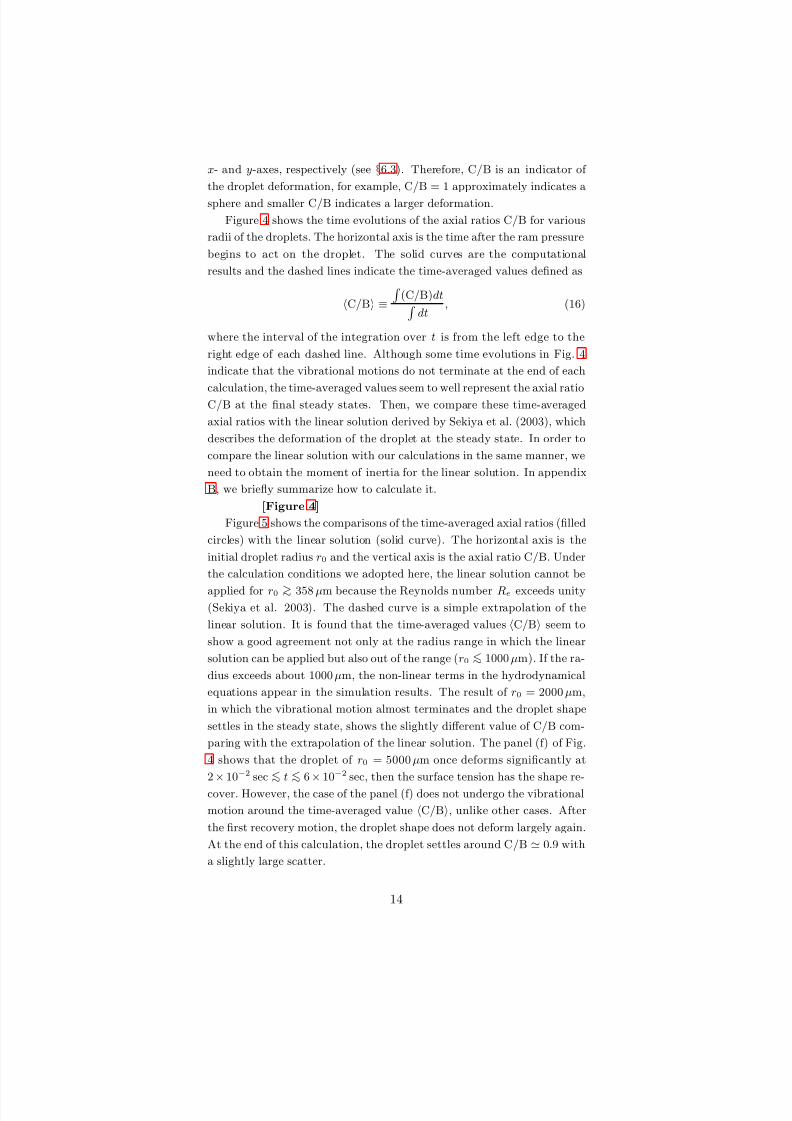
Figure 4 shows the time evolutions of the axial ratios C/B for various
radii of the droplets. The horizontal axis is the time after the ram pressure
begins to act on the droplet. The solid curves are the computational
results and the dashed lines indicate the time-averaged values defined as
C/B ≡
(C/B)dt dt
, (16)
where the interval of the integration over t is from the left edge to the
right edge of each dashed line. Although some time evolutions in Fig. 4
indicate that the vibrational motions do not terminate at the end of each
calculation, the time-averaged values seem to well represent the axial ratioC/B at the final steady states. Then, we compare these time-averaged
axial ratios with the linear solution derived by Sekiya et al. (2003), which
describes the deformation of the droplet at the steady state. In order to
compare the linear solution with our calculations in the same manner, we
need to obtain the moment of inertia for the linear solution. In appendix
B, we briefly summarize how to calculate it.
[Figure 4]
Figure 5 shows the comparisons of the time-averaged axial ratios (filled
circles) with the linear solution (solid curve). The horizontal axis is the
initial droplet radius r0 and the vertical axis is the axial ratio C/B. Under
the calculation conditions we adopted here, the linear solution cannot be
applied for r0 >∼ 358 µm because the Reynolds number Re exceeds unity(Sekiya et al. 2003). The dashed curve is a simple extrapolation of the
linear solution. It is found that the time-averaged values C/B seem to
show a good agreement not only at the radius range in which the linear
solution can be applied but also out of the range ( r0 <∼ 1000 µm). If the ra-
dius exceeds about 1000 µm, the non-linear terms in the hydrodynamical
equations appear in the simulation results. The result of r0 = 2000 µm,
in which the vibrational motion almost terminates and the droplet shape
settles in the steady state, shows the slightly different value of C/B com-
paring with the extrapolation of the linear solution. The panel (f) of Fig.
4 shows that the droplet of r0 = 5000 µm once deforms significantly at
2×
10−2 sec <
∼t <
∼6×
10−2 sec, then the surface tension has the shape re-
cover. However, the case of the panel (f) does not undergo the vibrational
motion around the time-averaged value C/B, unlike other cases. After
the first recovery motion, the droplet shape does not deform largely again.
At the end of this calculation, the droplet settles around C/B ≃ 0.9 with
a slightly large scatter.
14
8/14/2019 Shock-Wave Heating Model for Chondrule Formation
http://slidepdf.com/reader/full/shock-wave-heating-model-for-chondrule-formation 15/50
[Figure 5]
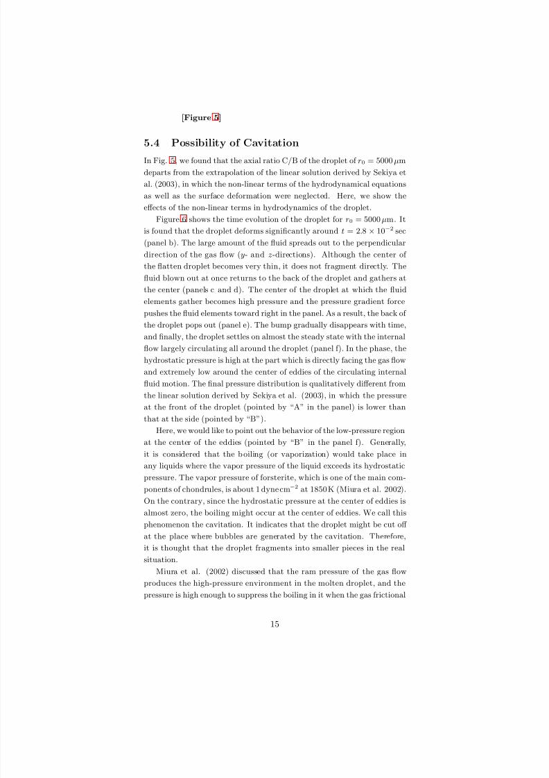
5.4 Possibility of Cavitation
In Fig. 5, we found that the axial ratio C/B of the droplet of r0 = 5000 µm
departs from the extrapolation of the linear solution derived by Sekiya et
al. (2003), in which the non-linear terms of the hydrodynamical equations
as well as the surface deformation were neglected. Here, we show the
effects of the non-linear terms in hydrodynamics of the droplet.
Figure 6 shows the time evolution of the droplet for r0 = 5000 µm. It
is found that the droplet deforms significantly around t = 2.8 × 10⁻² sec
(panel b). The large amount of the fluid spreads out to the perpendicular
direction of the gas flow (y- and z-directions). Although the center of
the flatten droplet becomes very thin, it does not fragment directly. The
fluid blown out at once returns to the back of the droplet and gathers at
the center (panels c and d). The center of the droplet at which the fluid
elements gather becomes high pressure and the pressure gradient force
pushes the fluid elements toward right in the panel. As a result, the back of
the droplet pops out (panel e). The bump gradually disappears with time,
and finally, the droplet settles on almost the steady state with the internal
flow largely circulating all around the droplet (panel f). In the phase, the
hydrostatic pressure is high at the part which is directly facing the gas flow
and extremely low around the center of eddies of the circulating internal
fluid motion. The final pressure distribution is qualitatively different from
the linear solution derived by Sekiya et al. (2003), in which the pressure
at the front of the droplet (pointed by “A” in the panel) is lower thanthat at the side (pointed by “B”).
Here, we would like to point out the behavior of the low-pressure region
at the center of the eddies (pointed by “B” in the panel f). Generally,
it is considered that the b oiling (or vaporization) would take place in
any liquids where the vapor pressure of the liquid exceeds its hydrostatic
pressure. The vapor pressure of forsterite, which is one of the main com-
ponents of chondrules, is about 1 dyne cm−2 at 1850 K (Miura et al. 2002).
On the contrary, since the hydrostatic pressure at the center of eddies is
almost zero, the boiling might occur at the center of eddies. We call this
phenomenon the cavitation. It indicates that the droplet might be cut off
at the place where bubbles are generated by the cavitation. Therefore,
it is thought that the droplet fragments into smaller pieces in the real
situation.
Miura et al. (2002) discussed that the ram pressure of the gas flow
produces the high-pressure environment in the molten droplet, and the
pressure is high enough to suppress the boiling in it when the gas frictional
15
8/14/2019 Shock-Wave Heating Model for Chondrule Formation
http://slidepdf.com/reader/full/shock-wave-heating-model-for-chondrule-formation 16/50
heating is strong enough to melt the silicate dust particles. However, they
did not take into account the hydrodynamics of the molten droplet. The
fragmentation by cavitation might be a new mechanism to explain the
maximum size of chondrules (see §6.1) like as the other mechanisms; the
fragmentation due to the gas flow directly (Susa & Nakamoto 2002) or the
stripping of the liquid surface in the gas flow (Kato et al. 2006, Kadono
& Arakawa 2005). To simulate the behavior of the bubbles generated in
the liquids should be the challenging task, but we think that such kind
of simulations are very important. It might be related with the existence
of holes in some chondrules (e.g., Kondo et al. 1997). It should be taken
into consideration in the future work.
[Figure 6]
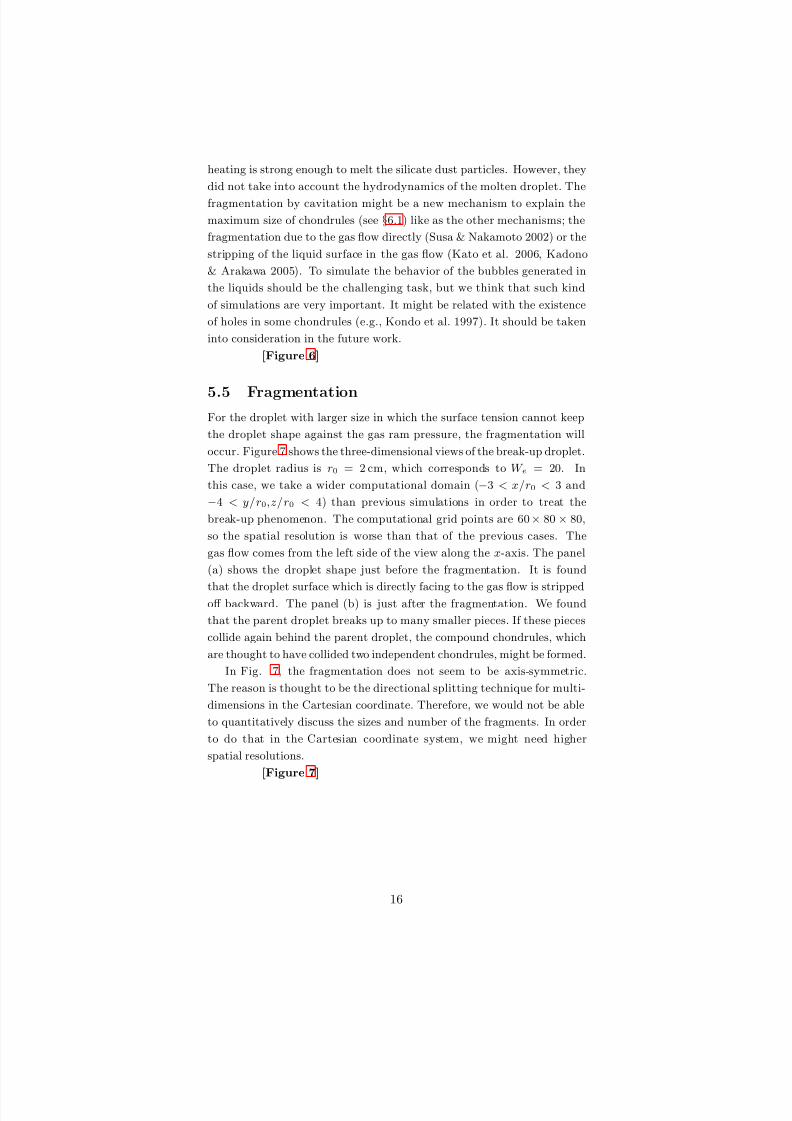
5.5 Fragmentation
For the droplet with larger size in which the surface tension cannot keep
the droplet shape against the gas ram pressure, the fragmentation will
occur. Figure 7 shows the three-dimensional views of the break-up droplet.
The droplet radius is r0 = 2 cm, which corresponds to W e = 20. In
this case, we take a wider computational domain (−3 < x/r0 < 3 and
−4 < y/r0,z/r0 < 4) than previous simulations in order to treat the
break-up phenomenon. The computational grid points are 60 × 80 × 80,
so the spatial resolution is worse than that of the previous cases. The
gas flow comes from the left side of the view along the x-axis. The panel
(a) shows the droplet shape just before the fragmentation. It is found
that the droplet surface which is directly facing to the gas flow is strippedoff backward. The panel (b) is just after the fragmentation. We found
that the parent droplet breaks up to many smaller pieces. If these pieces
collide again behind the parent droplet, the compound chondrules, which
are thought to have collided two independent chondrules, might be formed.
In Fig. 7, the fragmentation does not seem to be axis-symmetric.
The reason is thought to be the directional splitting technique for multi-
dimensions in the Cartesian coordinate. Therefore, we would not be able
to quantitatively discuss the sizes and number of the fragments. In order
to do that in the Cartesian coordinate system, we might need higher
spatial resolutions.
[Figure 7]
16
8/14/2019 Shock-Wave Heating Model for Chondrule Formation
http://slidepdf.com/reader/full/shock-wave-heating-model-for-chondrule-formation 17/50
6 Discussions
6.1 Maximum Size of Chondrules
Susa & Nakamoto (2002) suggested that the fragmentation of the droplets
in high-velocity gas flow limits the sizes of chondrules (upper limit). They
considered the balance between the surface tension and the inhomogene-
ity of the ram pressure acting on the droplet surface, and derived the
maximum size of molten silicate dust particles above which the droplet
would be destroyed by the ram pressure of the gas flow using an order of
magnitude estimation. In their estimation, they adopted the experimen-
tal data in which the droplets suddenly exposed to the gas flow fragment
for W e >∼ 6 (Bronshten 1983, p.96). This results into the fragmenta-
tion of droplet for r0 >
∼6000 µm if we adopt our calculation conditions
( pfm = 4000 dyne cm−2 and γ = 400dynecm−1).
On the contrary, our simulations showed the p ossibility that the droplets
fragment through the cavitation even if the radius is smaller than the max-
imum size derived by Susa & Nakamoto (2002) (see §5.4). The cavitation
would occur when the pressure gradient force cannot support the fluid
motion to circulate around the eddy. Here, we consider the condition
that the cavitation would take place using a simple order of magnitude
estimation. The pressure gradient force per unit volume can be estimated
as f pres ∼ p/(r0/2), where r0/2 indicates the radius of the eddy. On the
other hand, the centrifugal force for the fluid element circulating around
the eddy can be given as f cent ∼ ρdv2circ/(r0/2), where vcirc is the rota-
tional velocity. Balancing the pressure gradient and the centrifugal force
around the eddy, we have
p
r0/2∼ ρd
v2circ
r0/2. (17)
Substituting p = 2γ/r0 and vcirc ≃ vmax = 0.112 pfmr0/µd (Sekiya et al.
2003), we obtain
r0 ∼
2γµ2d
0.1122ρd p2fm
1/3
. (18)
This equation gives the critical radius of the droplet above which the
cavitation might occur in the center of the eddy and result into the frag-
mentation.
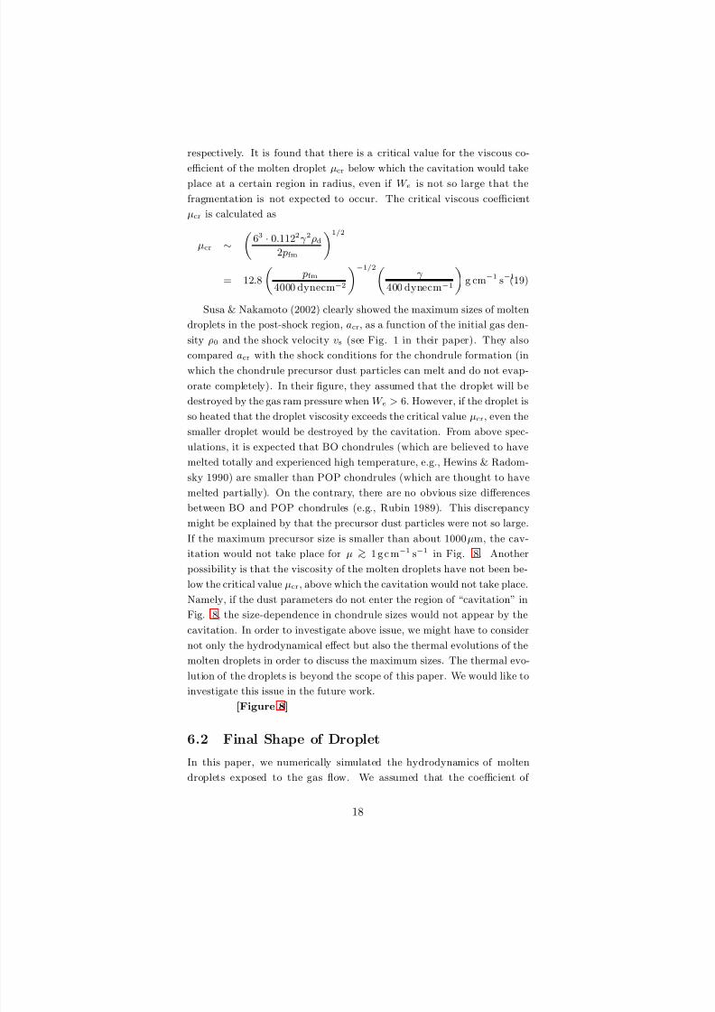
Figure 8 shows the two critical radii as a function of the viscosity;
the radius for W e = 6 (dotted line) and the radius at which the pres-
sure gradient force balances with the centrifugal force (dashed line). We
assume pfm = 4000 dynecm−2, γ = 400dynecm−1, and ρd = 3 g cm−3, re-
spectively. Our simulation results are also shown; not fragment (circles),
cavitation would take place (filled circles), and fragmentation (triangle),
17
8/14/2019 Shock-Wave Heating Model for Chondrule Formation
http://slidepdf.com/reader/full/shock-wave-heating-model-for-chondrule-formation 18/50
respectively. It is found that there is a critical value for the viscous co-
efficient of the molten droplet µcr below which the cavitation would take
place at a certain region in radius, even if W e is not so large that the
fragmentation is not expected to occur. The critical viscous coefficient
µcr is calculated as
µcr ∼
63 · 0.1122γ 2ρd
2 pfm
1/2
= 12.8
pfm
4000 dynecm−2
−1/2
γ
400 dynecm−1
g cm−1 s−1.(19)
Susa & Nakamoto (2002) clearly showed the maximum sizes of molten
droplets in the post-shock region, acr, as a function of the initial gas den-
sity ρ0 and the shock velocity vs (see Fig. 1 in their paper). They also
compared acr with the shock conditions for the chondrule formation (inwhich the chondrule precursor dust particles can melt and do not evap-
orate completely). In their figure, they assumed that the droplet will b e
destroyed by the gas ram pressure when W e > 6. However, if the droplet is
so heated that the droplet viscosity exceeds the critical value µcr, even the
smaller droplet would be destroyed by the cavitation. From above spec-
ulations, it is expected that BO chondrules (which are believed to have
melted totally and experienced high temperature, e.g., Hewins & Radom-
sky 1990) are smaller than POP chondrules (which are thought to have
melted partially). On the contrary, there are no obvious size differences
between BO and POP chondrules (e.g., Rubin 1989). This discrepancy
might be explained by that the precursor dust particles were not so large.
If the maximum precursor size is smaller than about 1000 µm, the cav-
itation would not take place for µ >∼ 1 g c m−1 s−1 in Fig. 8. Another
possibility is that the viscosity of the molten droplets have not been be-
low the critical value µcr, above which the cavitation would not take place.
Namely, if the dust parameters do not enter the region of “cavitation” in
Fig. 8, the size-dependence in chondrule sizes would not appear by the
cavitation. In order to investigate above issue, we might have to consider
not only the hydrodynamical effect but also the thermal evolutions of the
molten droplets in order to discuss the maximum sizes. The thermal evo-
lution of the droplets is beyond the scope of this paper. We would like to
investigate this issue in the future work.
[Figure 8]
6.2 Final Shape of Droplet
In this paper, we numerically simulated the hydrodynamics of molten
droplets exposed to the gas flow. We assumed that the coefficient of
18
8/14/2019 Shock-Wave Heating Model for Chondrule Formation
http://slidepdf.com/reader/full/shock-wave-heating-model-for-chondrule-formation 19/50
viscosity is constant in the droplets, and the droplets melt completely
and the physical conditions inside the droplets are homogeneous. On
the contrary, the shapes of chondrules are considered to be determined
around the re-solidification phase. Before the molten droplets re-solidify,
the droplet temperature falls down and the coefficient of viscosity would
change significantly. Moreover, if the droplets melt partially, the physical
conditions inside the droplets should not be homogeneous. Therefore, we
must discuss how we can consider above effects on the final shapes of
chondrules.
It is naturally considered that the viscosity of the droplet becomes
larger as the droplet temperature falls down. In such a lower Reynolds
number environment, the linear solution by Sekiya et al. (2003) is a
better approximation to describe the external shape and internal flow of
the droplet. According to their linear solution, the external shape of thedroplet does not depend on the viscosity. It indicates that the external
shape is determined mainly by the balance between the surface tension
and the gas ram pressure. Therefore, it is considered that the droplet
shape does not change significantly at the cooling phase in which the
viscosity of the droplet becomes higher and higher.
Another problem that we must take care for considering the droplet
shapes is inhomogeneity of the physical conditions in the droplet. For
example, if the dust particle is not heated enough, it would not melt
completely and the solid lumps floating in the droplet would exist. In
this case, the assumption of the completely molten droplet we adopted
loses the validity. However, if the external shape is significantly affected
by the solid lumps, the surface of chondrules should be irregular and
cannot be approximated by smoothed shapes (e.g., spheres or ellipsoids).
If considering conversely, it is thought that we can remove the above effect
by considering only the chondrules which have smooth surfaces. In fact,
there are some fraction of chondrules with smooth surfaces (Tsuchiyama et
al. 2003). Such chondrules would have melted almost completely, at least
the unmelted solid lumps do not affect the external shapes of droplets.
However, the majority of chondrules has the porphyritic texture, which
indicates that most of chondrule precursors did not completely melt in
the heating event (Hewins & Radomsky 1990). Moreover, iron sulfide
inclusions are observed in natural chondrules with various forms (Uesugi
et al. 2005). The unmelted clumps and the iron sulfide inclusions might
disturb the internal flow of the molten silicate particles2. This problem
2Uesugi et al. (2005) considered that the trajectories of the iron sulfide inclusions in
the silicate melts, however, they did not take into account the influence of the iron sulfide
inclusions on the flow pattern of the ambient silicate melt.
19
8/14/2019 Shock-Wave Heating Model for Chondrule Formation
http://slidepdf.com/reader/full/shock-wave-heating-model-for-chondrule-formation 20/50
is very complex and beyond the scope of this paper. We believe that this
problem can be investigated in the future.
6.3 Comparison with Chondrules
Tsuchiyama et al. (2003) studied three-dimensional shapes of chondrules
using X-ray microtomography. They measured twenty chondrules with
perfect shapes and smooth surfaces, which were selected from 47 chon-
drules separated from the Allende meteorite (CV3). The external shapes
were approximated as three-axial ellipsoids with a-, b-, and c-axes (axial
radii are A, B, and C (A ≥ B ≥ C), respectively) using the moments of
inertia of the chondrules, where the rotation axes with the minimum and
maximum moments correspond to the a- and c-axes, respectively. They
found that (1) the shapes are diverse from oblate (A∼
B > C), general
three-axial ellipsoid (A > B > C) to prolate chondrules (A > B ∼ C),
and (2) two groups can be recognized: oblate to prolate chondrules with
0.9 <∼ B/A <∼ 1.0 (group-A) and prolate chondrules with 0.74 <∼ B/A <∼0.80 (group-B).
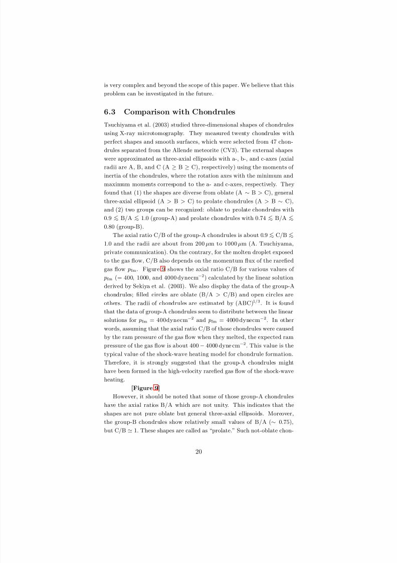
The axial ratio C/B of the group-A chondrules is about 0.9 <∼ C/B <∼1.0 and the radii are about from 200 µm to 1000 µm (A. Tsuchiyama,
private communication). On the contrary, for the molten droplet exposed
to the gas flow, C/B also depends on the momentum flux of the rarefied
gas flow pfm. Figure 9 shows the axial ratio C/B for various values of
pfm (= 400, 1000, and 4000 dynecm−2) calculated by the linear solution
derived by Sekiya et al. (2003). We also display the data of the group-A
chondrules; filled circles are oblate (B/A > C/B) and open circles areothers. The radii of chondrules are estimated by (ABC)1/3. It is found
that the data of group-A chondrules seem to distribute between the linear
solutions for pfm = 400dynecm−2 and pfm = 4000 dynecm−2. In other
words, assuming that the axial ratio C/B of those chondrules were caused
by the ram pressure of the gas flow when they melted, the expected ram
pressure of the gas flow is about 400 − 4000 dyne cm−2. This value is the
typical value of the shock-wave heating model for chondrule formation.
Therefore, it is strongly suggested that the group-A chondrules might
have been formed in the high-velocity rarefied gas flow of the shock-wave
heating.
[Figure 9]
However, it should be noted that some of those group-A chondrules
have the axial ratios B/A which are not unity. This indicates that the
shapes are not pure oblate but general three-axial ellipsoids. Moreover,
the group-B chondrules show relatively small values of B/A (∼ 0.75),
but C/B ≃ 1. These shapes are called as “prolate.” Such not-oblate chon-
20
8/14/2019 Shock-Wave Heating Model for Chondrule Formation
http://slidepdf.com/reader/full/shock-wave-heating-model-for-chondrule-formation 21/50
drules cannot be explained considering only the effect of the ram pressure.
In order to produce the not-oblate molten droplet, we must investigate
other effects which give some dynamical effect to the droplet (e.g., rotation
of the droplet). In our forthcoming paper, we are planing to investigate
the rapidly rotating droplets exposed to the gas flow. The dust rotation
causes the three-dimensional deformation depending on the rotation axis.
Therefore, the analysis based on the assumption of axis-symmetry would
not be used. Since our numerical code has been developed on the concept
of the three-dimension, any special improvements are not required for the
application to the rapidly rotating droplets.
6.4 Ram Pressure at Re-solidification?
The precursor dust particles moving through the nebula gas are deceler-
ated by the ram pressure of the gas flow. Therefore, the relative velocity
vrel between them becomes small with time. It indicates that the gas ram
pressure pfm = ρgv2rel at the time when the molten droplet re-solidifies
would be smaller than that when it melts first.
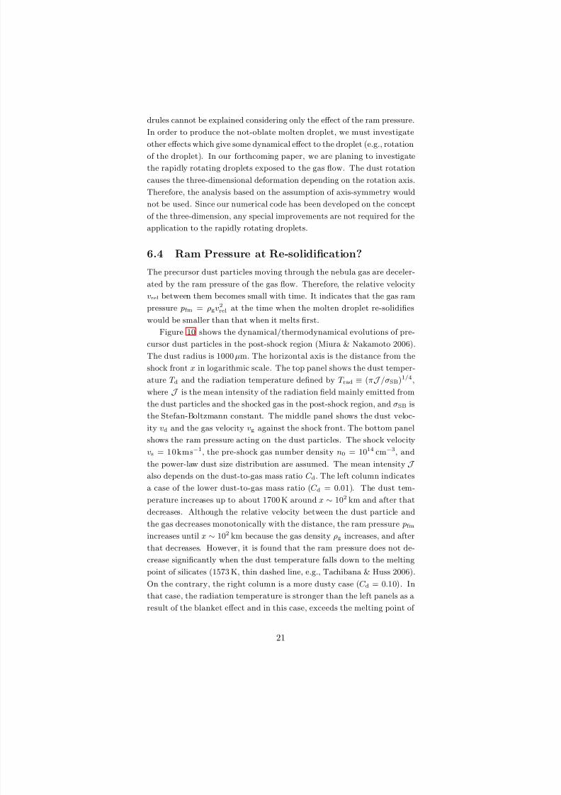
Figure 10 shows the dynamical/thermodynamical evolutions of pre-
cursor dust particles in the post-shock region (Miura & Nakamoto 2006).
The dust radius is 1000 µm. The horizontal axis is the distance from the
shock front x in logarithmic scale. The top panel shows the dust temper-
ature T d and the radiation temperature defined by T rad ≡ (πJ /σSB)1/4,
where J is the mean intensity of the radiation field mainly emitted from
the dust particles and the shocked gas in the post-shock region, and σSB is
the Stefan-Boltzmann constant. The middle panel shows the dust veloc-ity vd and the gas velocity vg against the shock front. The bottom panel
shows the ram pressure acting on the dust particles. The shock velocity
vs = 10kms−1, the pre-shock gas number density n0 = 1014 cm−3, and
the power-law dust size distribution are assumed. The mean intensity J also depends on the dust-to-gas mass ratio C d. The left column indicates
a case of the lower dust-to-gas mass ratio (C d = 0.01). The dust tem-
perature increases up to about 1700 K around x ∼ 102 km and after that
decreases. Although the relative velocity between the dust particle and
the gas decreases monotonically with the distance, the ram pressure pfm
increases until x ∼ 102 km because the gas density ρg increases, and after
that decreases. However, it is found that the ram pressure does not de-
crease significantly when the dust temperature falls down to the melting
point of silicates (1573 K, thin dashed line, e.g., Tachibana & Huss 2006).
On the contrary, the right column is a more dusty case (C d = 0.10). In
that case, the radiation temperature is stronger than the left panels as a
result of the blanket effect and in this case, exceeds the melting point of
21
8/14/2019 Shock-Wave Heating Model for Chondrule Formation
http://slidepdf.com/reader/full/shock-wave-heating-model-for-chondrule-formation 22/50
silicates. Since the dust particles are also heated by the radiation field,
they do not cool even if the relative velocity is almost zero. They can
cool if the radiation field becomes weak. At that time, the ram pressure
has not already taken place on the dust particles. To summarize, the ram
pressure acting on the re-solidifing molten droplet can take various values
depending on the shock conditions and dust models in the chondrule-
forming region. Generally, the low dust-to-gas mass environment would
result into the large ram pressure.
[Figure 10]
6.5 Dust Particle Rotation
We investigated the hydrodynamics of molten droplet exposed to the gas
flow. However, in the shock-wave heating model, the situation where the
rapidly rotating droplets are exposed to the high-velocity gas flow can be
considered. Some possibilities for the origin of the dust rotation can be
considered, for example, the net torque when the droplet fragments by
the gas ram pressure (Susa & Nakamoto 2002), the interaction between
the dust particles and the ambient gas flow, and the dust-dust collision.
Therefore, we have to take into account the effect of the rotation. When
the rotation axis is perpendicular to the gas flow, the three-dimensional
effect is expected in the droplet shapes. Our code has been already devel-
oped in the concept of the three-dimensional calculations. We are planing
to examine the case that the rotating droplets are exposed to the high-
velocity gas flow in our forthcoming paper.
7 Conclusions
We have developed the non-linear, time-dependent, and three-dimensional
hydrodynamic simulation code in order to investigate the hydrodynamics
of molten droplets exposed to the high-velocity rarefied gas flow. Our
numerical code is based on the concept of the CIP scheme, guarantees the
exact mass conservation, and additionally, we introduced the anti-diffusion
technique for suppressing the effect of the numerical diffusion at the dis-
continuity in density. We carried out the simulations for various droplet
radii (r0 = 100 µm − 2 cm). The other physical parameters were adopted
typical values for the shock-wave heating condition (the momentum of
molecular gas flow pfm = 4000 dynecm−2) and the silicate melts (surface
tension γ = 400dynecm−1, coefficient of viscosity µd = 1.3 g c m−1 s−1).
We conclude as follows:
1. Since we considered that the gas ram pressure suddenly affects the
22
8/14/2019 Shock-Wave Heating Model for Chondrule Formation
http://slidepdf.com/reader/full/shock-wave-heating-model-for-chondrule-formation 23/50
initially spherical droplet, the droplets whose radii are smaller than
5000 µm showed the vibrational motion (deformation by the ram
pressure and recovery motion by the surface tension). The vibration
gradually dissipates by the viscosity and the droplets tend to settle
in the steady states.
2. The degree of the deformation at the steady state (or time-averaged
value) showed a good agreement with the linear solution derived by
Sekiya et al. (2003) if the droplet radii are smaller than 1000 µm.
For larger droplets, the final shapes are far from the linear solu-
tion because the non-linear term in the hydrodynamical equation
dominates, which terms were ignored in the derivation of the linear
solution.
3. If the droplet radii are larger than 5000 µm, the hydrostatic pressure
inside the eddies of the droplet internal flow becomes almost zero.
In this region, the phase transition from liquid to vapor would occur
and some bubbles would be generated in the droplet (cavitation).
It is considered that the cavitation causes the fragmentation of the
droplets.
4. When the droplet radius is larger than 1 cm, the droplet fragments
directly by the gas ram pressure. We found that the parent droplet
breaks up to many smaller pieces. If these pieces collide again behind
the parent droplet, the compound chondrules, which are thought to
have collided two independent chondrules, might be formed.
5. We considered that the fragmentation through the cavitation might
be a new mechanism to determine the maximum size of chondrules.
Using the order of magnitude estimation, we found that the cavi-
tation can easily occur in the low-viscosity droplets. We discussed
the possibility that this relation can explain why chondrules in some
carbonaceous chondrites are smaller than that in other chondrites.
6. We compared our simulation results of the molten droplets with
chondrules measured by Tsuchiyama et al. (2003) in the external
shape, and found that the variety of chondrule shapes cannot be re-
produced only by the effect of the ram pressure of the gas flow. We
pointed out the importance of other mechanisms, e.g., the rotation
of the droplets.
Acknowledgments:
We greatly appreciate Prof. Akira Tsuchiyama for his helpful comments
and offering the observational data of chondrules. We are also grateful to
23
8/14/2019 Shock-Wave Heating Model for Chondrule Formation
http://slidepdf.com/reader/full/shock-wave-heating-model-for-chondrule-formation 24/50
Dr. Hidemi Mutsuda for many useful information about the CIP scheme
described in his doctor thesis. HM was supported by the Research Fellow-
ship of Japan Society for the Promotion of Science for Young Scientists.
TN was partially supported by the Ministry of Education, Science, Sports
and Culture, Grant-in-Aid for Scientific Research (C), 1754021.
A Numerical Method in Hydrodynamics
In this appendix, we briefly explain the strategies of the numerical schemes
that we adopted in our model. The hydrodynamical equations except for
the equation of continuity were separated into two phases; the advection
phase (§A.1) and the non-advection phase (§A.2). The equation of conti-
nuity was solved in the conservative form (
§A.1.2). We also describe the
method to keep the incompressibility of the fluid in §A.3 and the modelparameters we adopted in this study in §A.4.
A.1 Advection Phase
A.1.1 CIP scheme
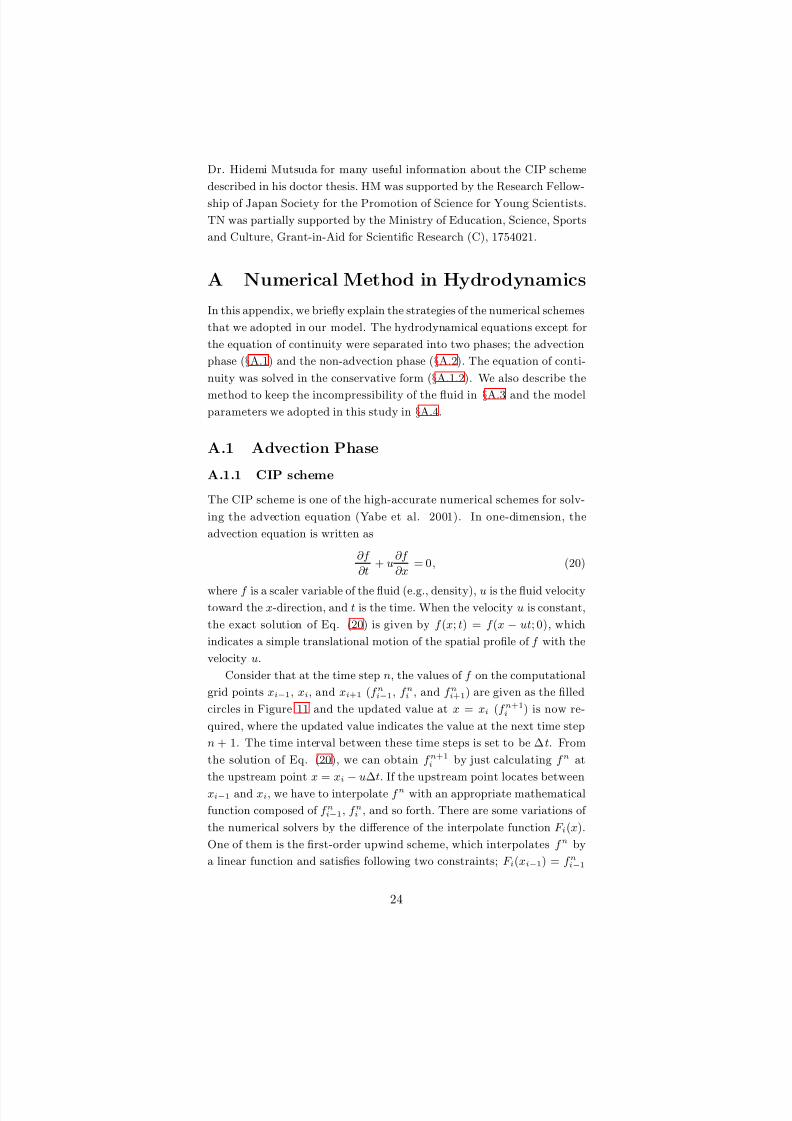
The CIP scheme is one of the high-accurate numerical schemes for solv-
ing the advection equation (Yabe et al. 2001). In one-dimension, the
advection equation is written as
∂f
∂t+ u
∂f
∂x= 0, (20)
where f is a scaler variable of the fluid (e.g., density), u is the fluid velocitytoward the x-direction, and t is the time. When the velocity u is constant,
the exact solution of Eq. (20) is given by f (x; t) = f (x − ut; 0), which
indicates a simple translational motion of the spatial profile of f with the
velocity u.
Consider that at the time step n, the values of f on the computational
grid points xi−1, xi, and xi+1 (f ni−1, f ni , and f ni+1) are given as the filled
circles in Figure 11 and the updated value at x = xi (f n+1i ) is now re-
quired, where the updated value indicates the value at the next time step
n + 1. The time interval between these time steps is set to be ∆t. From
the solution of Eq. (20), we can obtain f n+1i by just calculating f n at
the upstream point x = xi−
u∆t. If the upstream point locates between
xi−1 and xi, we have to interpolate f n with an appropriate mathematical
function composed of f ni−1, f ni , and so forth. There are some variations of
the numerical solvers by the difference of the interpolate function F i(x).
One of them is the first-order upwind scheme, which interpolates f n by
a linear function and satisfies following two constraints; F i(xi−1) = f ni−1
24
8/14/2019 Shock-Wave Heating Model for Chondrule Formation
http://slidepdf.com/reader/full/shock-wave-heating-model-for-chondrule-formation 25/50
and F i(xi) = f ni . The other variation is the Lax-Wendroff scheme, which
uses a quadratic polynomial satisfying three constraints; F i(xi−1) = f ni−1,
F i(xi) = f ni , and F i(xi+1) = f ni+1.
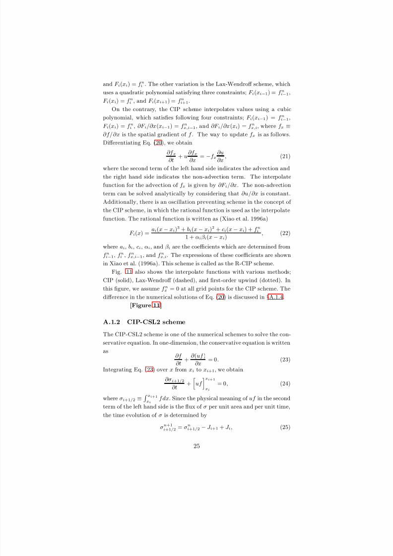
On the contrary, the CIP scheme interpolates values using a cubic
polynomial, which satisfies following four constraints; F i(xi−1) = f ni−1,
F i(xi) = f ni , ∂F i/∂x(xi−1) = f nx,i−1, and ∂F i/∂x(xi) = f nx,i, where f x ≡∂f/∂x is the spatial gradient of f . The way to update f x is as follows.
Differentiating Eq. (20), we obtain
∂f x∂t
+ u∂f x∂x
= −f x∂u
∂x, (21)
where the second term of the left hand side indicates the advection and
the right hand side indicates the non-advection term. The interpolate
function for the advection of f x is given by ∂F i/∂x. The non-advection
term can be solved analytically by considering that ∂u/∂x is constant.Additionally, there is an oscillation preventing scheme in the concept of
the CIP scheme, in which the rational function is used as the interpolate
function. The rational function is written as (Xiao et al. 1996a)
F i(x) =ai(x − xi)
3 + bi(x − xi)2 + ci(x − xi) + f ni
1 + αiβ i(x − xi), (22)
where ai, bi, ci, αi, and β i are the coefficients which are determined from
f ni−1, f ni , f nx,i−1, and f nx,i. The expressions of these coefficients are shown
in Xiao et al. (1996a). This scheme is called as the R-CIP scheme.
Fig. 11 also shows the interpolate functions with various methods;
CIP (solid), Lax-Wendroff (dashed), and first-order upwind (dotted). In
this figure, we assume f nx
= 0 at all grid points for the CIP scheme. The
difference in the numerical solutions of Eq. (20) is discussed in §A.1.4.
[Figure 11]
A.1.2 CIP-CSL2 scheme
The CIP-CSL2 scheme is one of the numerical schemes to solve the con-
servative equation. In one-dimension, the conservative equation is written
as∂f
∂t+
∂ (uf )
∂x= 0. (23)
Integrating Eq. (23) over x from xi to xi+1, we obtain
∂σi+1/2
∂t
+ uf xi+1
xi
= 0, (24)
where σi+1/2 ≡ xi+1xi
fdx. Since the physical meaning of uf in the second
term of the left hand side is the flux of σ per unit area and per unit time,
the time evolution of σ is determined by
σn+1i+1/2 = σn
i+1/2 − J i+1 + J i, (25)
25
8/14/2019 Shock-Wave Heating Model for Chondrule Formation
http://slidepdf.com/reader/full/shock-wave-heating-model-for-chondrule-formation 26/50
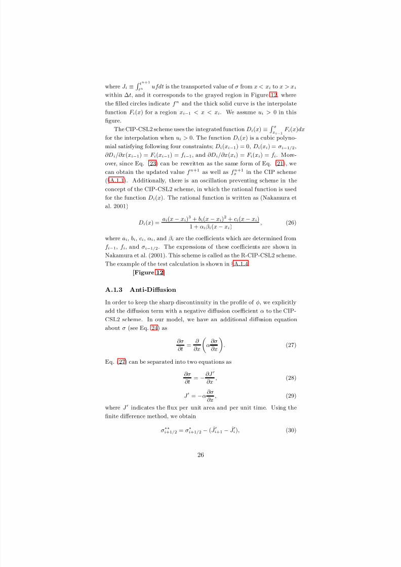
where J i ≡ tn+1
tnufdt is the transported value of σ from x < xi to x > xi
within ∆t, and it corresponds to the grayed region in Figure 12, where
the filled circles indicate f n and the thick solid curve is the interpolate
function F i(x) for a region xi−1 < x < xi. We assume ui > 0 in this
figure.
The CIP-CSL2 scheme uses the integrated function Di(x) ≡ xxi−1
F i(x)dx
for the interpolation when ui > 0. The function Di(x) is a cubic polyno-
mial satisfying following four constraints; Di(xi−1) = 0, Di(xi) = σi−1/2,
∂Di/∂x(xi−1) = F i(xi−1) = f i−1, and ∂Di/∂x(xi) = F i(xi) = f i. More-
over, since Eq. (23) can be rewritten as the same form of Eq. (21), we
can obtain the updated value f n+1 as well as f n+1x in the CIP scheme
(§A.1.1). Additionally, there is an oscillation preventing scheme in the
concept of the CIP-CSL2 scheme, in which the rational function is used
for the function Di(x). The rational function is written as (Nakamura etal. 2001)
Di(x) =ai(x − xi)
3 + bi(x − xi)2 + ci(x − xi)
1 + αiβ i(x − xi), (26)
where ai, bi, ci, αi, and β i are the coefficients which are determined from
f i−1, f i, and σi−1/2. The expressions of these coefficients are shown in
Nakamura et al. (2001). This scheme is called as the R-CIP-CSL2 scheme.
The example of the test calculation is shown in §A.1.4.
[Figure 12]
A.1.3 Anti-Diffusion
In order to keep the sharp discontinuity in the profile of φ, we explicitly
add the diffusion term with a negative diffusion coefficient α to the CIP-
CSL2 scheme. In our model, we have an additional diffusion equation
about σ (see Eq. 24) as
∂σ
∂t=
∂
∂x
α
∂σ
∂x
. (27)
Eq. (27) can be separated into two equations as
∂σ
∂t= −∂J ′
∂x, (28)
J ′
= −α
∂σ
∂x , (29)
where J ′ indicates the flux per unit area and per unit time. Using the
finite difference method, we obtain
σ∗∗
i+1/2 = σ∗
i+1/2 − (J ′i+1 − J ′i), (30)
26
8/14/2019 Shock-Wave Heating Model for Chondrule Formation
http://slidepdf.com/reader/full/shock-wave-heating-model-for-chondrule-formation 27/50
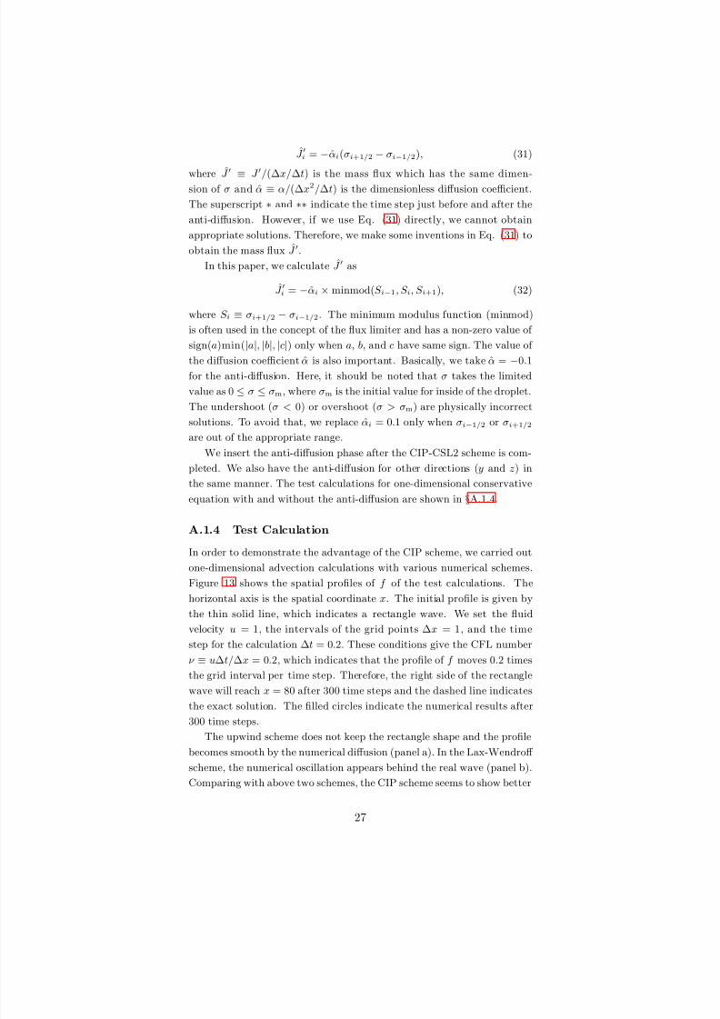
J ′i = −αi(σi+1/2 − σi−1/2), (31)
whereˆ
J
′
≡ J
′
/(∆x/∆t) is the mass flux which has the same dimen-sion of σ and α ≡ α/(∆x2/∆t) is the dimensionless diffusion coefficient.
The superscript ∗ and ∗∗ indicate the time step just before and after the
anti-diffusion. However, if we use Eq. (31) directly, we cannot obtain
appropriate solutions. Therefore, we make some inventions in Eq. (31) to
obtain the mass flux J ′.
In this paper, we calculate J ′ as
J ′i = −αi × minmod(S i−1, S i, S i+1), (32)
where S i ≡ σi+1/2 − σi−1/2. The minimum modulus function (minmod)
is often used in the concept of the flux limiter and has a non-zero value of
sign(a)min(
|a
|,
|b
|,
|c
|) only when a, b, and c have same sign. The value of
the diffusion coefficient α is also important. Basically, we take α = −0.1
for the anti-diffusion. Here, it should be noted that σ takes the limited
value as 0 ≤ σ ≤ σm, where σm is the initial value for inside of the droplet.
The undershoot (σ < 0) or overshoot (σ > σm) are physically incorrect
solutions. To avoid that, we replace αi = 0.1 only when σi−1/2 or σi+1/2
are out of the appropriate range.
We insert the anti-diffusion phase after the CIP-CSL2 scheme is com-
pleted. We also have the anti-diffusion for other directions (y and z) in
the same manner. The test calculations for one-dimensional conservative
equation with and without the anti-diffusion are shown in §A.1.4.
A.1.4 Test CalculationIn order to demonstrate the advantage of the CIP scheme, we carried out
one-dimensional advection calculations with various numerical schemes.
Figure 13 shows the spatial profiles of f of the test calculations. The
horizontal axis is the spatial coordinate x. The initial profile is given by
the thin solid line, which indicates a rectangle wave. We set the fluid
velocity u = 1, the intervals of the grid points ∆x = 1, and the time
step for the calculation ∆t = 0.2. These conditions give the CFL number
ν ≡ u∆t/∆x = 0.2, which indicates that the profile of f moves 0.2 times
the grid interval per time step. Therefore, the right side of the rectangle
wave will reach x = 80 after 300 time steps and the dashed line indicates
the exact solution. The filled circles indicate the numerical results after
300 time steps.
The upwind scheme does not keep the rectangle shape and the profile
becomes smooth by the numerical diffusion (panel a). In the Lax-Wendroff
scheme, the numerical oscillation appears behind the real wave (panel b).
Comparing with above two schemes, the CIP scheme seems to show better
27
8/14/2019 Shock-Wave Heating Model for Chondrule Formation
http://slidepdf.com/reader/full/shock-wave-heating-model-for-chondrule-formation 28/50
solution, however, some undershoots (f < 0) or overshoots (f > 1) are
observed in the numerical result (panel c). In the R-CIP scheme, although
the faint numerical diffusion has still remained, we obtain the excellent
solution comparing with the exact solution (panel d).
We also show the numerical results of the one-dimensional conservative
equation (Eq. 23). We use the same conditions with the one-dimensional
advection equation (Eq. 20). Note that Eq. (23) corresponds to Eq. (20)
when the velocity u is constant. The panel (e) shows the results of the
R-CIP-CSL2 scheme, which is similar to that of the R-CIP scheme. In
the panel (f), we found that the combination of the R-CIP-CSL2 scheme
and the anti-diffusion technique (§A.1.3) shows the excellent solution in
which the numerical diffusion is prevented effectively.
[Figure 13]
A.2 Non-Advection Phase
A.2.1 C-CUP scheme
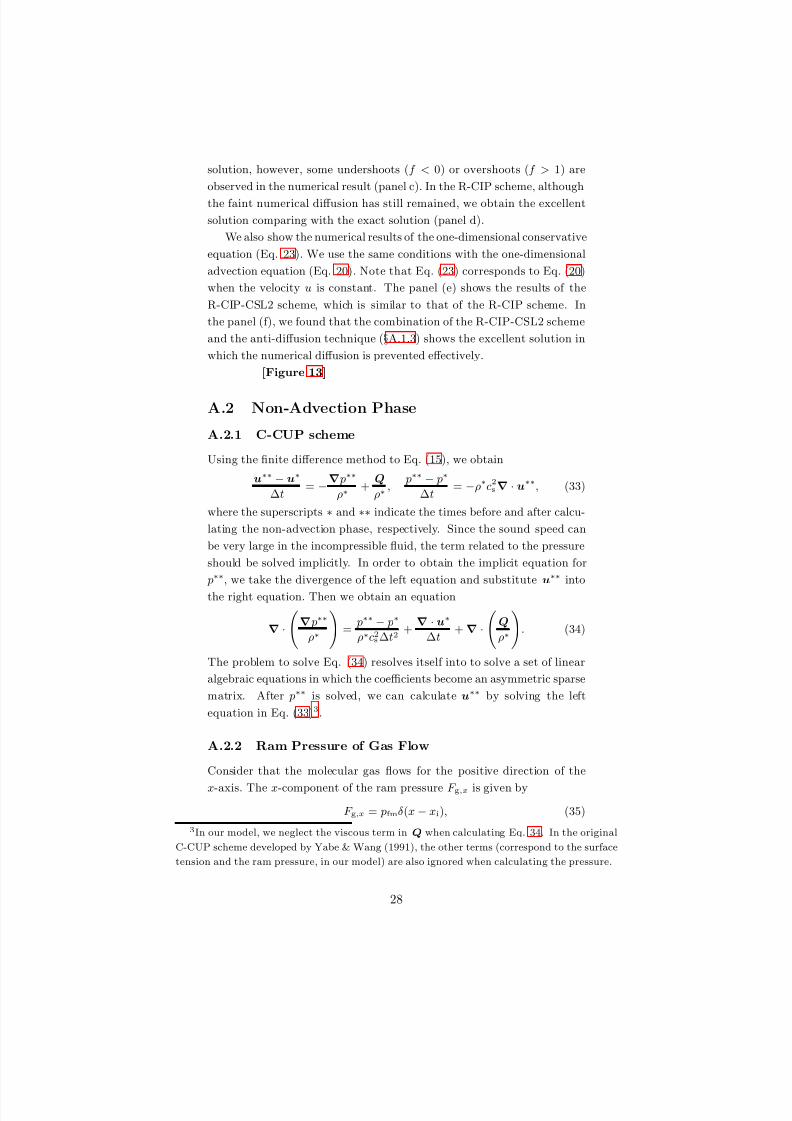
Using the finite difference method to Eq. (15), we obtain
u∗∗ − u∗
∆t= −∇ p∗∗
ρ∗+
Q
ρ∗,
p∗∗ − p∗
∆t= −ρ∗c2s∇ · u∗∗, (33)
where the superscripts ∗ and ∗∗ indicate the times before and after calcu-
lating the non-advection phase, respectively. Since the sound speed can
be very large in the incompressible fluid, the term related to the pressure
should be solved implicitly. In order to obtain the implicit equation for
p∗∗, we take the divergence of the left equation and substitute u∗∗ into
the right equation. Then we obtain an equation
∇ ·∇ p∗∗
ρ∗
=
p∗∗− p∗
ρ∗c2s∆t2+∇ · u∗
∆t+∇ ·
Q
ρ∗
. (34)
The problem to solve Eq. (34) resolves itself into to solve a set of linear
algebraic equations in which the coefficients become an asymmetric sparse
matrix. After p∗∗ is solved, we can calculate u∗∗ by solving the left
equation in Eq. (33)3.
A.2.2 Ram Pressure of Gas Flow
Consider that the molecular gas flows for the positive direction of the
x-axis. The x-component of the ram pressure F g,x is given by
F g,x = pfmδ(x − xi), (35)
3In our model, we neglect the viscous term in Q when calculating Eq. 34. In the original
C-CUP scheme developed by Yabe & Wang (1991), the other terms (correspond to the surface
tension and the ram pressure, in our model) are also ignored when calculating the pressure.
28
8/14/2019 Shock-Wave Heating Model for Chondrule Formation
http://slidepdf.com/reader/full/shock-wave-heating-model-for-chondrule-formation 29/50
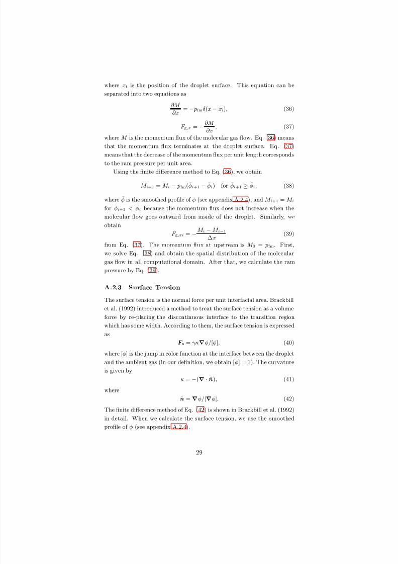
where xi is the position of the droplet surface. This equation can be
separated into two equations as
∂M
∂x= − pfmδ(x − xi), (36)
F g,x = −∂M
∂x, (37)
where M is the momentum flux of the molecular gas flow. Eq. (36) means
that the momentum flux terminates at the droplet surface. Eq. (37)
means that the decrease of the momentum flux per unit length corresponds
to the ram pressure per unit area.
Using the finite difference method to Eq. (36), we obtain
M i+1 = M i − pfm(φi+1 − φi) for φi+1 ≥ φi, (38)
where φ is the smoothed profile of φ (see appendix A.2.4), and M i+1 = M i
for φi+1 < φi because the momentum flux does not increase when the
molecular flow goes outward from inside of the droplet. Similarly, we
obtain
F g,xi = −M i − M i−1
∆x(39)
from Eq. (37). The momentum flux at upstream is M 0 = pfm. First,
we solve Eq. (38) and obtain the spatial distribution of the molecular
gas flow in all computational domain. After that, we calculate the ram
pressure by Eq. (39).
A.2.3 Surface Tension
The surface tension is the normal force per unit interfacial area. Brackbill
et al. (1992) introduced a method to treat the surface tension as a volume
force by re-placing the discontinuous interface to the transition region
which has some width. According to them, the surface tension is expressed
as
F s = γκ∇φ/[φ], (40)
where [φ] is the jump in color function at the interface between the droplet
and the ambient gas (in our definition, we obtain [ φ] = 1). The curvature
is given by
κ = −(∇ · n), (41)
where
n =∇φ/|∇φ|. (42)
The finite difference method of Eq. (42) is shown in Brackbill et al. (1992)
in detail. When we calculate the surface tension, we use the smoothed
profile of φ (see appendix A.2.4).
29
8/14/2019 Shock-Wave Heating Model for Chondrule Formation
http://slidepdf.com/reader/full/shock-wave-heating-model-for-chondrule-formation 30/50
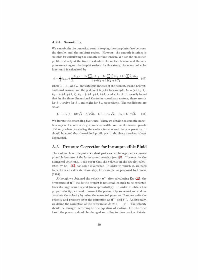
A.2.4 Smoothing
We can obtain the numerical results keeping the sharp interface betweenthe droplet and the ambient region. However, the smooth interface is
suitable for calculating the smooth surface tension. We use the smoothed
profile of φ only at the time to calculate the surface tension and the ram
pressure acting on the droplet surface. In this study, the smoothed color
function φ is calculated by
φ =1
2φi,j,k +
1
2
φi,j,k + C 16
L1φL1 + C 2
12
L2φL2 + C 3
8
L3φL3
1 + 6C 1 + 12C 2 + 8C 3, (43)
where L1, L2, and L3 indicate grid indexes of the nearest, second nearest,
and third nearest from the grid point (i,j,k), for example, L1 = (i+1, j , k),
L2 = (i+1, j+1, k), L3 = (i+1, j+1, k+1), and so forth. It is easily found
that in the three-dimensional Cartesian coordinate system, there are sixfor L1, twelve for L2, and eight for L3, respectively. The coefficients are
set as
C 1 = 1/(6 + 12/√
2 + 8/√
3), C 2 = C 1/√
2, C 3 = C 1/√
3. (44)
We iterate the smoothing five times. Then, we obtain the smooth transi-
tion region of about twice grid interval width. We use the smooth profile
of φ only when calculating the surface tension and the ram pressure. It
should be noted that the original profile φ with the sharp interface is kept
unchanged.
A.3 Pressure Correction for Incompressible FluidThe molten chondrule precursor dust particles can be regarded as incom-
pressible because of the large sound velocity (see §2). However, in the
numerical solutions, it can occur that the velocity in the droplet calcu-
lated by Eq. (33) has some divergence. In order to vanish it, we need
to perform an extra iteration step, for example, as proposed by Chorin
(1968).
Although we obtained the velocity u∗∗ after calculating Eq. (33), the
divergence of u∗∗ inside the droplet is not small enough to be expected
from its large sound speed (incompressibility). In order to obtain the
proper velocity, we need to correct the pressure by some method and re-
calculate the velocity by using the corrected pressure. Here, we write thevelocity and pressure after the correction as u∗∗ and ˜ p∗∗. Additionally,
we define the correction of the pressure as δp ≡ ˜ p∗∗ − p∗∗. The velocity
should be changed according to the equation of motion. On the other
hand, the pressure should be changed according to the equation of state.
30
8/14/2019 Shock-Wave Heating Model for Chondrule Formation
http://slidepdf.com/reader/full/shock-wave-heating-model-for-chondrule-formation 31/50
Therefore, we have the velocity/pressure correction method as (c.f., Eq.
33)u∗∗ − u∗∗
∆t= −∇δp
ρ∗, ˜ p∗∗ − p∗∗
∆t= −ρ∗c2s∇ · u∗∗. (45)
We iterate these equations until ˜ p∗∗ converges. The same numerical
scheme as applied for Eq. (33) can be used to solve Eq. (45).
A.4 Model Parameters
In Table 1, parameters marked by (*) have no physical meanings. These
values are empirical settings for the numerical simulation.
While we set the density of the ambient region ρa = 10−6 g cm−3, the
typical gas density of the protoplanetary disk is ∼ 10−9 g cm−3 in the
minimum mass solar nebula (Hayashi et al. 1985). There is a difference
of about four orders of magnitude in the densities, however, the numericalresults do not depend significantly on the ambient density because it is
too small to affect the dynamics of the molten droplet. The stronger
the density contrast between the droplet and the ambient region is, the
more difficult the numerical simulation becomes. From above reasons, we
adopted the relatively large value for the ambient density in the numerical
simulation.
While we set the sound speed of the ambient region cs,a = 10−5 cm s−1,
the typical value of the disk gas is cs,disk ≃ (kBT /mH2)1/2 ≃ 105 cm s−1,
where kB is the Stefan-Boltzmann constant, T is the gas temperature (we
substitute T = 300 K), and mH2is the molecular weight of H2. Remember
that in this study, the disk gas around the molten droplet behaves like as
a free molecular flow and does not follow the hydrodynamical equations
(§2). Therefore, we do not need to consider the sound wave and the
pressure change by the compression/expansion in the ambient region. We
thought that the extremely low sound speed for the ambient region is one
of the appropriate ways to express above features in the concept of the
multi-fluids analysis.
Finally, we set the viscous coefficient of the ambient region µa =
10−2 g cm−1 s−1 because it should not be zero for the stability of the cal-
culations.
B Moment of Inertia for Linear Solution
The external shapes obtained by our numerical simulations were approxi-
mated as three-axial ellipsoids using the moments of inertia. We compared
our results with the linear solution derived by Sekiya et al. (2003) in this
paper. When we obtain the axial ratio of the linear solution, the moment
31
8/14/2019 Shock-Wave Heating Model for Chondrule Formation
http://slidepdf.com/reader/full/shock-wave-heating-model-for-chondrule-formation 32/50
of inertia for the linear solution is needed. It can be calculated using the
formalism by Sekiya et al. (2003) as follows.
Sekiya et al. (2003) gave the distance between the dust surface to
the origin of the spherical coordinates4 as rs(θ) = r0(1 + W exs(θ)), where
W e = pfmr0/γ is the Weber number, θ is the angle from the radius of
droplet to the negative x-direction in our coordinate, and xs is the dimen-
sionless parameter which was given as a function of θ. The expression of
xs is given in Sekiya et al. (2003). The moment of inertia around the
x-axis is calculated as
I xx = ρd
rs(θ)0
dr
π0
dθ
2π0
dψ(r sin θ)2r2 sin θ,
=2
5πρdr5
0
5
m=0
5PmbmW me , (46)
where P is the permutation defined by nPr ≡ n!/(n − r)! and
bm ≡ π0
xms (θ)sin3 θdθ. (47)
We obtain b0 = 4/3. It can be easily confirmed that I xx has the same value
of a sphere (I = (8/15)πρdr50) when W e = 0. For other coefficients, we
calculate using an appropriate numerical integration method and obtain
b1 = 0.42222 × 10⁻¹, b2 = 0.51562 × 10⁻², b3 = 0.74446 × 10⁻⁴, b4 =
0.44106 × 10⁻⁴, and b5 = −0.28485 × 10⁻⁵.
4Sekiya et al. (2003) chose the origin of the spherical coordinates as drs/dθ = 0 at θ = π/2.
32
8/14/2019 Shock-Wave Heating Model for Chondrule Formation
http://slidepdf.com/reader/full/shock-wave-heating-model-for-chondrule-formation 33/50
References
[1] Amelin, Y., Krot, A. N., Hutcheon, I. D., & Ulyanov, A. A., 2002.Lead Isotopic Ages of Chondrules and Calcium-Aluminum-Rich In-
clusions. Science 297, 1678-1683.
[2] Boss, A. P., 1996. A Concise Cuide to Chondrule Formation Models.
In: Hewins, R. H., Jones, R., & Scott, R. D. (Eds.), Chondrules and
the Protoplanetary Disk, Cambridge Univ. Press, Cambridge, pp.
257-263.
[3] Bottinga, Y., & Weill, D. F., 1972. The viscosity of magmatic silicate
liquids; a model for calculation. Americal Journal of Science 272, 438-
475.
[4] Brackbill, J. U., Kothe, D. B., & Zemach, C., 1992. A continuum
method for modeling surface tension. J. Comp. Phys. 100, 335-354.
[5] Bronshten, V. A. 1983. Physics of Meteoric Phenomena. D. Reidel
Publishing Company, Holland.
[6] Chorin, A. J., 1968. Numerical Solution of the Navier-Stokes Equa-
tions. Mathematics of Computation 22, 745-762.
[7] Ciesla, F. J., & Hood, L. L., 2002. The Nebular Shock Wave Model
for Chondrule Formation: Shock Processing in a Particle-Gas Sus-
pension. Icarus 158, 281-293.
[8] Desch, S. J., & Connolly, H. C., Jr., 2002. A model of the thermal
processing of particles in solar nebula shocks: Application to the
cooling rates of chondrules. Meteorit. Planet. Sci. 37, 183-207.
[9] Hayashi, C., Nakazawa, K., & Nakagawa, Y., 1985. Formation of the
solar system. In: Black, D. C., & Matthews, M. S. (Eds.), Protostars
and Planets II, Univ. Arizona Press, Tucson, pp. 1100-1153.
[10] Hewins, R. H., & Radomsky, P. M., 1990. Temperature conditions
for chondrule formation. Meteoritics 25, 309-318.
[11] Hollenbach, D., & McKee, C. F., 1979. Molecule formation and in-
frared emission in fast interstellar shocks. The Astrophysical Journal
Supplement Series 41, 555-592.
[12] Hood, L. L., 1998. Thermal processing of chondrule and CAI precur-
sors in planetesimal bow shocks. Meteorit. Planet. Sci. 33, 97-107.
[13] Hood, L. L., & Horanyi, M., 1991. Gas dynamic heating of chondrule
precursor grains in the solar nebula. Icarus 93, 259-269.
[14] Hood, L. L., & Horanyi, M., 1993. The nebular shock wave model
for chondrule formation — One-dimensional calculations. Icarus 106,
179-189.
33
8/14/2019 Shock-Wave Heating Model for Chondrule Formation
http://slidepdf.com/reader/full/shock-wave-heating-model-for-chondrule-formation 34/50
[15] Iida, A., Nakamoto, T., Susa, H., & Nakagawa, Y., 2001. A Shock
Heating Model for Chondrule Formation in a Protoplanetary Disk.
Icarus 153, 430-450.
[16] Jones, R. H., Lee, T., Connolly, H. C., Jr., Love, S. G., & Shang, H.,
2000. Formation of Chondrules and CAIs: Theory vs. Observation.
In: Boss, A. P., & Russell, S. S. (Eds.), Protostars and Planets IV,
Univ. Arizona Press, Tucson, pp. 927-962.
[17] Kadono, T., & Arakawa, M., 2005. Breakup of liquids by high velocity
flow and size distribution of chondrules. Icarus 173, 295-299.
[18] Kato, T., Nakamoto, T., & Miura, H., 2006. Maximal Size of Chon-
drules in Shock Wave Heating Model: Stripping of Liquid Surface in
a Hypersonic Rarefied Gas Flow. Meteorit. Planet. Sci. 41, 49-65.
[19] Kondo, M., Tsuchiyama, A., Hirai, H., & Koishikawa, A., 1997. Highresolution X-ray computed tomographic (CT) images of chondrites
and a chondrule. Antarctic Meteorite Res. 10, 437-447.
[20] Landau, L. D., & Lifshitz, E. M., 1987. Fluid mechanics. –2nd
ed.– (Course of theoretical physics; v. 6). Elsevier Butterworth-
Heinemann, Oxford, UK. p. 45.
[21] Miura, H., Nakamoto, T., & Susa, H., 2002. A Shock-Wave Heating
Model for Chondrule Formation: Effects of Evaporation and Gas
Flows on Silicate Particles. Icarus 160, 258-270.
[22] Miura, H., & Nakamoto, T., 2005. A shock-wave heating model for
chondrule formation II. Minimum size of chondrule precursors. Icarus
175, 289-304.[23] Miura, H., & Nakamoto, T., 2006. Shock-wave heating model for
chondrule formation: Prevention of Isotopic Fractionation. Astro-
phys. J. 651, 1272.
[24] Murase, T., & McBirney, A. R., 1973. Properties of Some Common
Igneous Rocks and Their Melts at High Temperatures. Geol. Soc.
Am. Bull. 84, 3563-3592.
[25] Nakamura, T., Tanaka, R., Yabe, T., & Takizawa, K., 2001. Exactly
Conservative Semi-Lagrangian Scheme for Multi-dimensional Hyper-
bolic Equations with Directional Splitting Technique. J. Comp. Phys.
174, 171-207.
[26] Rubin, A. E., & Keil, K., 1984. Size-distributions of chondrule types
in the Inman and Allan Hills A77011 L3 chondrites. Meteoritics 19,
135-143.
[27] Rubin, A. E., 1989. Size-frequency distributions of chondrules in CO3
chondrites. Meteoritics 24, 179-189.
34
8/14/2019 Shock-Wave Heating Model for Chondrule Formation
http://slidepdf.com/reader/full/shock-wave-heating-model-for-chondrule-formation 35/50
8/14/2019 Shock-Wave Heating Model for Chondrule Formation
http://slidepdf.com/reader/full/shock-wave-heating-model-for-chondrule-formation 36/50
[40] Xiao, F., & Ikebata, A., 2003. An efficient method for capturing free
boundaries in multi-fluid simulations. Int. J. Numer. Meth. Fluids
42, 187-210.
36
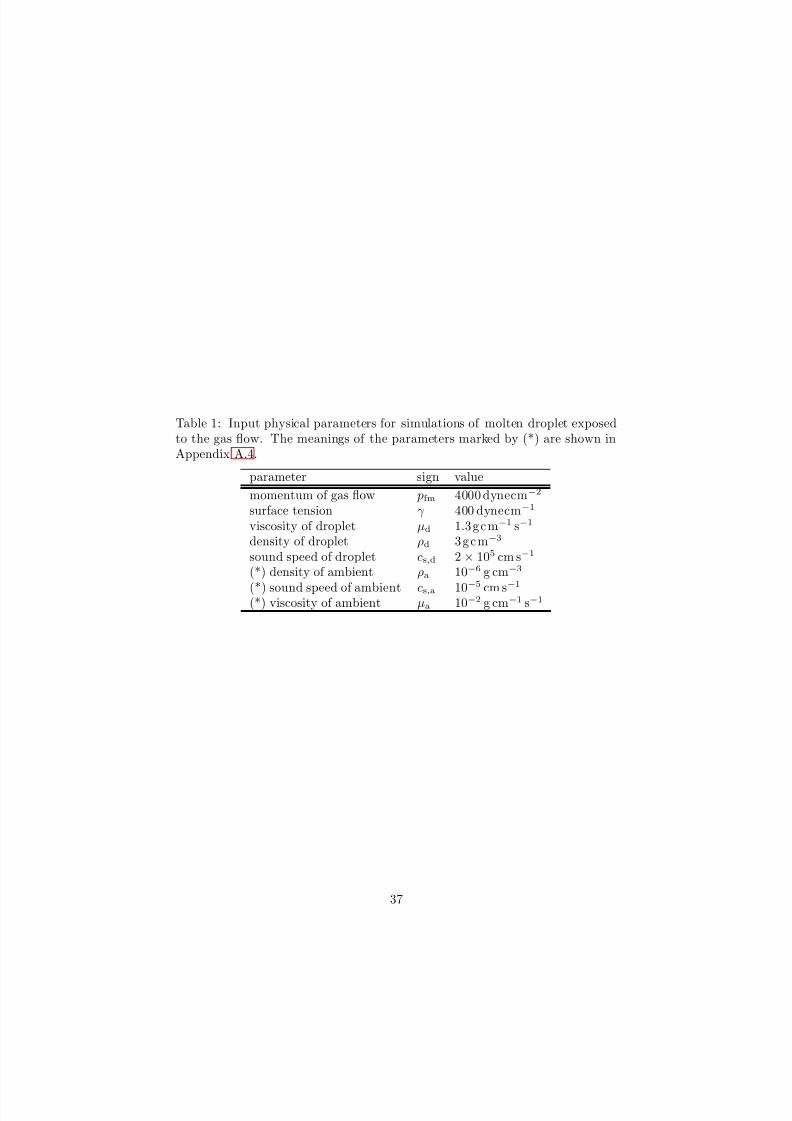
8/14/2019 Shock-Wave Heating Model for Chondrule Formation
http://slidepdf.com/reader/full/shock-wave-heating-model-for-chondrule-formation 37/50
Table 1: Input physical parameters for simulations of molten droplet exposedto the gas flow. The meanings of the parameters marked by (*) are shown inAppendix A.4.
parameter sign value
momentum of gas flow pfm 4000 dynecm−2
surface tension γ 400 dynecm−1
viscosity of droplet µd 1.3 g c m−1 s−1
density of droplet ρd 3 g c m−3
sound speed of droplet cs,d 2× 105 cm s−1
(*) density of ambient ρa 10−6 g cm−3
(*) sound speed of ambient cs,a 10−5
cm s−1
(*) viscosity of ambient µa 10−2 g cm−1 s−1
37
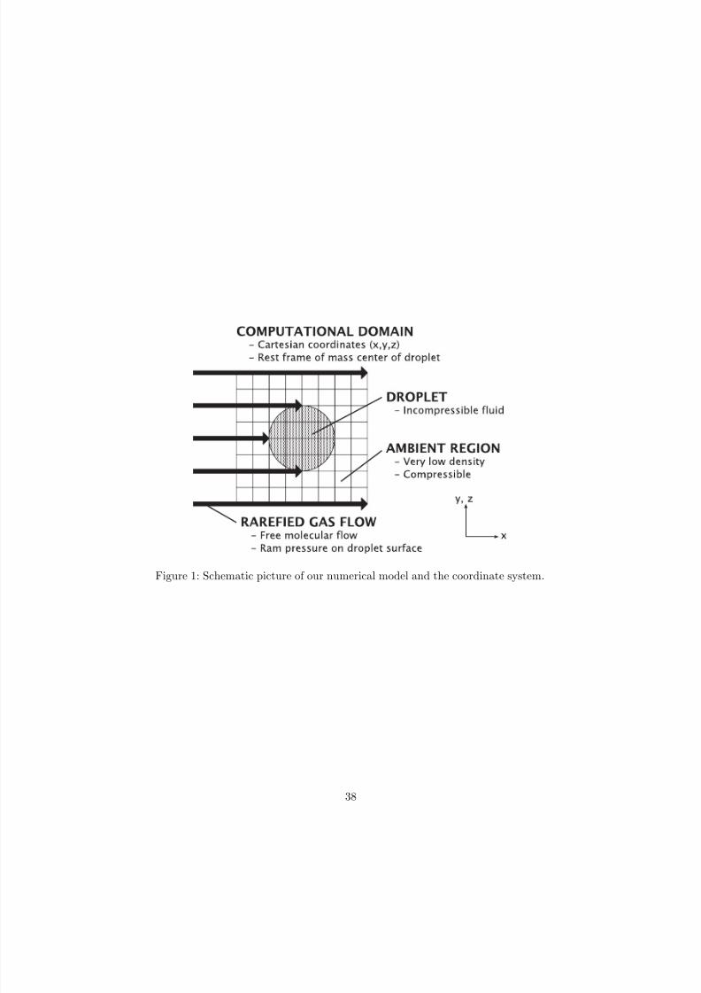
8/14/2019 Shock-Wave Heating Model for Chondrule Formation
http://slidepdf.com/reader/full/shock-wave-heating-model-for-chondrule-formation 38/50
Figure 1: Schematic picture of our numerical model and the coordinate system.
38
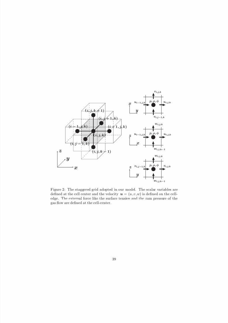
8/14/2019 Shock-Wave Heating Model for Chondrule Formation
http://slidepdf.com/reader/full/shock-wave-heating-model-for-chondrule-formation 39/50
y
z
x
y
z
y
x
z
x
(i− 1, j, k)
(i, j − 1, k)
(i, j, k− 1)
i, j, k)
(i + 1, j, k)
(i, j + 1, k)
i, j, k + 1)
ui−1,j,k ui,j,k
ui,j,kui−1,j,k
vi,j,k
vi,j−1,k
vi,j,kvi,j−1,k
wi,j,k
wi,j,k−1
wi,j,k
wi,j,k−1
p,ρ,φ
p,ρ,φ
p,ρ,φ
Figure 2: The staggered grid adopted in our model. The scalar variables aredefined at the cell center and the velocity u = (u,v,w) is defined on the cell-edge. The external force like the surface tension and the ram pressure of thegas flow are defined at the cell-center.
39
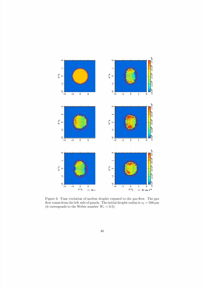
8/14/2019 Shock-Wave Heating Model for Chondrule Formation
http://slidepdf.com/reader/full/shock-wave-heating-model-for-chondrule-formation 40/50
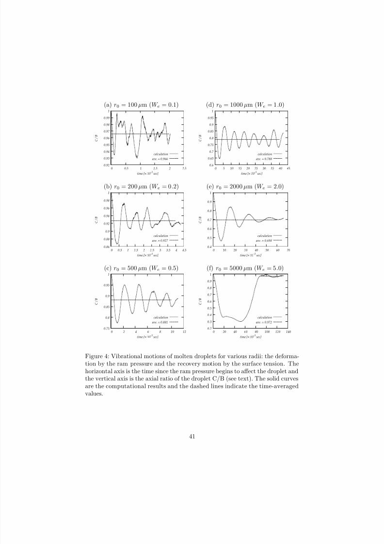
8/14/2019 Shock-Wave Heating Model for Chondrule Formation
http://slidepdf.com/reader/full/shock-wave-heating-model-for-chondrule-formation 41/50
(a) r0 = 100µm (W e = 0.1)
0.92
0.93
0.94
0.95
0.96
0.97
0.98
0.99
1
0 0.5 1 1.5 2 2.5
C /
B
time [× 10-3
sec]
calculation
ave. = 0.966
(d) r0 = 1000µm (W e = 1.0)
0.6
0.65
0.7
0.75
0.8
0.85
0.9
0.95
1
0 5 10 15 20 25 30 35 40 45
C /
B
time [× 10-3
sec]
calculation
ave. = 0.788
(b) r0 = 200µm (W e = 0.2)
0.86
0.88
0.9
0.92
0.94
0.96
0.98
1
0 0.5 1 1.5 2 2.5 3 3.5 4 4.5
C /
B
time [× 10-3
sec]
calculation
ave. = 0.927
(e) r0 = 2000µm (W e = 2.0)
0.4
0.5
0.6
0.7
0.8
0.9
1
0 10 20 30 40 50 60 70
C /
B
time [× 10-3
sec]
calculation
ave. = 0.698
(c) r0 = 500µm (W e = 0.5)
0.75
0.8
0.85
0.9
0.95
1
0 2 4 6 8 10 12
C /
B
time [× 10-3
sec]
calculation
ave. = 0.881
(f) r0 = 5000µm (W e = 5.0)
0.2
0.3
0.4
0.5
0.6
0.7
0.8
0.9
1
0 20 40 60 80 100 120 140
C /
B
time [× 10-3
sec]
calculation
ave. = 0.972
Figure 4: Vibrational motions of molten droplets for various radii: the deforma-tion by the ram pressure and the recovery motion by the surface tension. Thehorizontal axis is the time since the ram pressure begins to affect the droplet and
the vertical axis is the axial ratio of the droplet C/B (see text). The solid curvesare the computational results and the dashed lines indicate the time-averagedvalues.
41
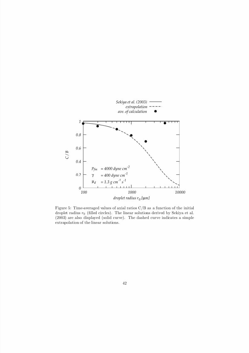
8/14/2019 Shock-Wave Heating Model for Chondrule Formation
http://slidepdf.com/reader/full/shock-wave-heating-model-for-chondrule-formation 42/50
0
0.2
0.4
0.6
0.8
1
100 1000 10000
C /
B
droplet radius r0 [µm]
p fm
γ
µd
= 4000 dyne cm-2
= 400 dyne cm-1
= 1.3 g cm-1 s-1
Sekiya et al. (2003)extrapolation
ave. of calculation
Figure 5: Time-averaged values of axial ratios C/B as a function of the initialdroplet radius r0 (filled circles). The linear solutions derived by Sekiya et al.(2003) are also displayed (solid curve). The dashed curve indicates a simpleextrapolation of the linear solutions.
42
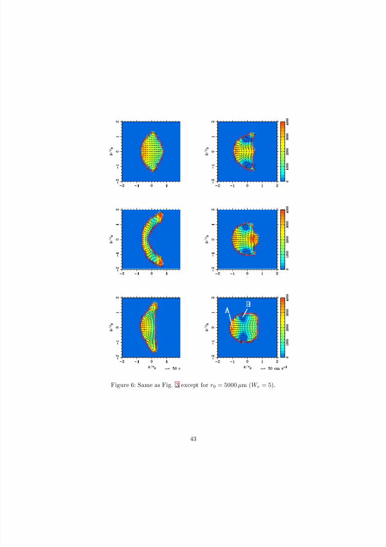
8/14/2019 Shock-Wave Heating Model for Chondrule Formation
http://slidepdf.com/reader/full/shock-wave-heating-model-for-chondrule-formation 43/50
(a) 11 msec (d) 71 msec
(b) 28 msec (e) 79 msec
(c) 62 msec (f) 107 msec
Figure 6: Same as Fig. 3 except for r0 = 5000µm (W e = 5).
43
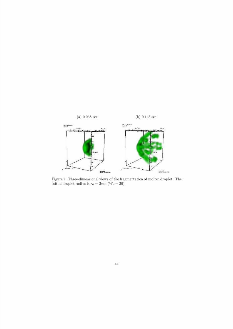
8/14/2019 Shock-Wave Heating Model for Chondrule Formation
http://slidepdf.com/reader/full/shock-wave-heating-model-for-chondrule-formation 44/50
(a) 0.068 sec (b) 0.143 sec
Figure 7: Three-dimensional views of the fragmentation of molten droplet. Theinitial droplet radius is r0 = 2cm (W e = 20).
44
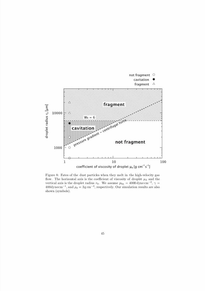
8/14/2019 Shock-Wave Heating Model for Chondrule Formation
http://slidepdf.com/reader/full/shock-wave-heating-model-for-chondrule-formation 45/50
Figure 8: Fates of the dust particles when they melt in the high-velocity gasflow. The horizontal axis is the coefficient of viscosity of droplet µd and thevertical axis is the droplet radius r0. We assume pfm = 4000 dyne cm−2, γ =400dynecm−1, and ρd = 3g cm−3, respectively. Our simulation results are alsoshown (symbols).
45
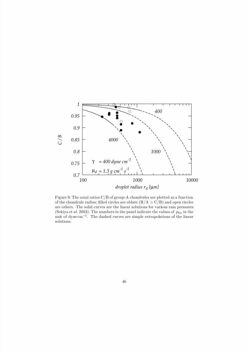
8/14/2019 Shock-Wave Heating Model for Chondrule Formation
http://slidepdf.com/reader/full/shock-wave-heating-model-for-chondrule-formation 46/50
0.7
0.75
0.8
0.85
0.9
0.95
1
100 1000 10000
C /
B
droplet radius r0 [µm]
γ
µd
= 400 dyne cm-1
= 1.3 g cm-1
s-1
4000
1000
400
Figure 9: The axial ratios C/B of group-A chondrules are plotted as a functionof the chondrule radius; filled circles are oblate (B/A > C/B) and open circlesare others. The solid curves are the linear solutions for various ram pressures(Sekiya et al. 2003). The numbers in the panel indicate the values of pfm in theunit of dyne cm−2. The dashed curves are simple extrapolations of the linearsolutions.
46
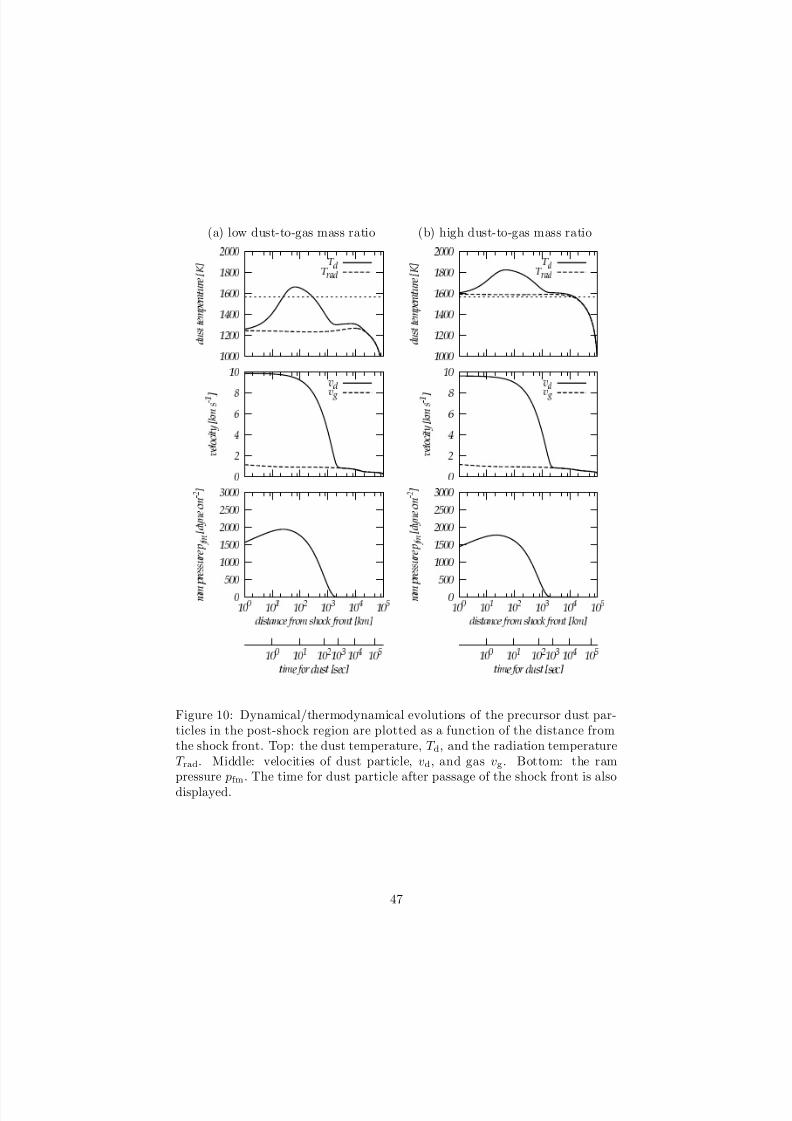
8/14/2019 Shock-Wave Heating Model for Chondrule Formation
http://slidepdf.com/reader/full/shock-wave-heating-model-for-chondrule-formation 47/50
(a) low dust-to-gas mass ratio (b) high dust-to-gas mass ratio
Figure 10: Dynamical/thermodynamical evolutions of the precursor dust par-ticles in the post-shock region are plotted as a function of the distance fromthe shock front. Top: the dust temperature, T d, and the radiation temperatureT rad. Middle: velocities of dust particle, vd, and gas vg. Bottom: the rampressure pfm. The time for dust particle after passage of the shock front is alsodisplayed.
47
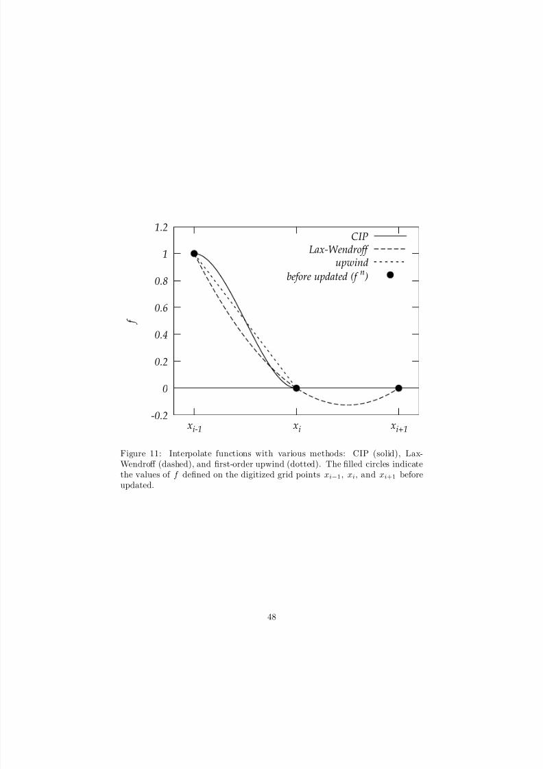
8/14/2019 Shock-Wave Heating Model for Chondrule Formation
http://slidepdf.com/reader/full/shock-wave-heating-model-for-chondrule-formation 48/50
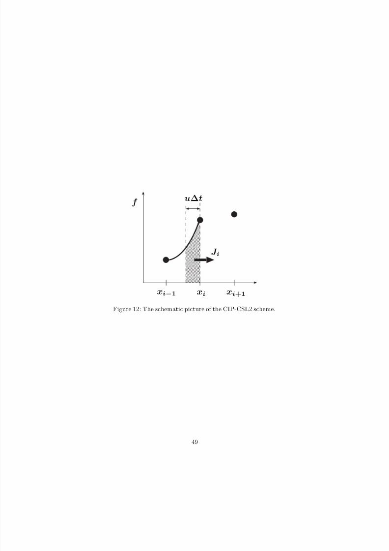
8/14/2019 Shock-Wave Heating Model for Chondrule Formation
http://slidepdf.com/reader/full/shock-wave-heating-model-for-chondrule-formation 49/50
f
xi−1 xi+1xi
u∆t
J i
Figure 12: The schematic picture of the CIP-CSL2 scheme.
49
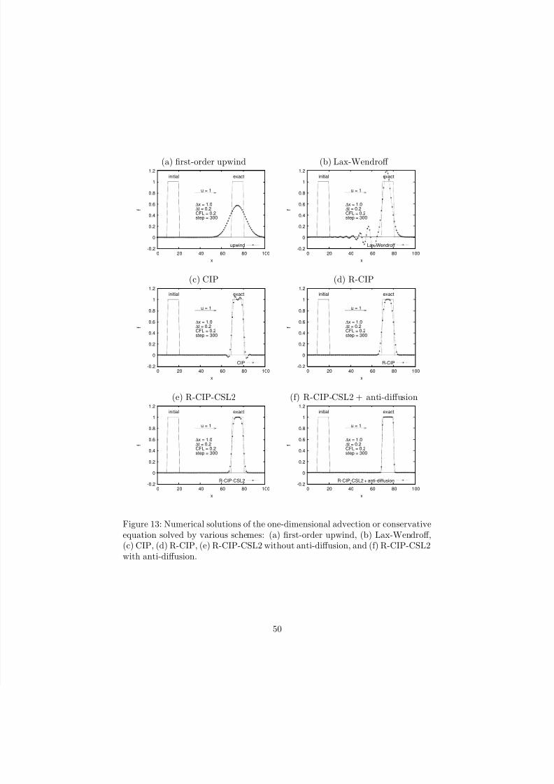
8/14/2019 Shock-Wave Heating Model for Chondrule Formation
http://slidepdf.com/reader/full/shock-wave-heating-model-for-chondrule-formation 50/50