Embed Size (px)
Citation preview

arX
iv:1
912.
0571
2v2
[m
ath.
OC
] 7
Apr
202
0
Short simplex paths in lattice polytopes
Alberto Del Pia ∗ Carla Michini †
April 9, 2020
Abstract
The goal of this paper is to design a simplex algorithm for linear programs onlattice polytopes that traces ‘short’ simplex paths from any given vertex to an optimalone. We consider a lattice polytope P contained in [0, k]n and defined via m linearinequalities. Our first contribution is a simplex algorithm that reaches an optimalvertex by tracing a path along the edges of P of length in O(n4k log(nk)). The lengthof this path is independent from m and it is the best possible up to a polynomialfunction. In fact, it is only polynomially far from the worst-case diameter, whichroughly grows as a linear function in n and k.
Motivated by the fact that most known lattice polytopes are defined via 0,±1constraint matrices, our second contribution is an iterative algorithm which exploitsthe largest absolute value α of the entries in the constraint matrix. We show that thelength of the simplex path generated by the iterative algorithm is in O(n2k log(nkα)).In particular, if α is bounded by a polynomial in n, k, then the length of the simplexpath is in O(n2k log(nk)).
For both algorithms, the number of arithmetic operations needed to compute thenext vertex in the path is polynomial in n, m and log k. If k is polynomially boundedby n and m, the algorithm runs in strongly polynomial time.
Key words: lattice polytopes; simplex algorithm; diameter; strongly polynomial time
1 Introduction
Linear programming (LP) is one of the most fundamental types of optimization models.In an LP problem, we are given a polyhedron P ⊆ Rn and a cost vector c ∈ Zn, and wewish to solve the optimization problem
maxc⊤x | x ∈ P. (1)
The polyhedron P is explicitly given via a system of linear inequalities, i.e., P = x ∈Rn | Ax ≤ b, where A ∈ Zm×n, b ∈ Zm. If P is nonempty and bounded, problem (1)admits an optimal solution that is a vertex of P .
∗Department of Industrial and Systems Engineering & Wisconsin Institute for Discovery, University of
Wisconsin-Madison, Madison, WI, USA. E-mail: [email protected].†Department of Industrial and Systems Engineering, University of Wisconsin-Madison, Madison, WI,
USA. E-mail: [email protected].
1

In this paper, we consider a special class of linear programs (1) where the feasibleregion is a lattice polytope, i.e., a polytope whose vertices have integer coordinates. Thesepolytopes are particularly relevant in discrete optimization and integer programming, asthey correspond to the convex hull of the feasible solutions to such optimization problems.In particular, a [0, k]-polytope in Rn is defined as a lattice polytope contained in the box[0, k]n.
One of the main algorithms for LP is the simplex method. The simplex method movesfrom the current vertex to an adjacent one along an edge of the polyhedron P , until anoptimal vertex is reached or unboundedness is detected, and the selection of the next vertexdepends on a pivoting rule. The sequence of vertices generated by the simplex method iscalled the simplex path. The main objective of this paper is to design a simplex algorithmfor [0, k]-polytopes that constructs ‘short’ simplex paths from any starting vertex x0.
But how short can a simplex path be? A natural lower bound on the length of asimplex path from x0 to x∗ is given by the distance between these two vertices, whichis defined as the minimum length of a path connecting x0 and x∗ along the edges of thepolyhedron P . The diameter of P is the largest distance between any two vertices ofP , and therefore it provides a lower bound on the length of a worst-case simplex pathon P . It is known that the diameter of [0, 1]-polytopes in Rn is at most n [22] and thisbound is attained by the hypercube [0, 1]n. This upper bound was later generalized tonk for general [0, k]-polytopes in Rn [18], and refined to n
⌊
(k − 12 )⌋
for k ≥ 2 [8] and tonk−
⌈
23n
⌉
− (k−3) for k ≥ 3 [10]. For k = 2 the bound given in [8] is tight. In general, forfixed k, the diameter of lattice polytopes can grow linearly with n, since there are latticepolytopes, called primitive zonotopes, that can have diameter in Ω(n) [9]. Viceversa, whenn is fixed, the diameter of a [0, k]-polytope in Rn can grow almost linearly with k. In fact,it is known that for n = 2 there are [0, k]-polytopes with diameter in Ω(k2/3) [4, 27, 1].
Moreover, for any fixed n, there are primitive zonotopes with diameter in Ω(kn
n+1 ) for kthat goes to infinity [11].
Can we design a simplex algorithm whose simplex path length is only polynomiallyfar from optimal, meaning that it is upper bounded by a polynomial function of theworst-case diameter? In this paper, we answer this question in the affermative. Our firstcontribution is a preprocessing & scaling algorithm that generates a simplex path of lengthin O(n4k log(nk)) for [0, k]-polytopes in Rn. The length of the simplex path is indeedpolynomially far from optimal, as it is polynomially bounded in n and k. We remark thatthe upper bound is independent on m. This is especially interesting because, even for[0, 1]-polytopes, m can grow exponentially in n (see, e.g., [24]).
Our next objective is that of decreasing the gap between the length O(n4k log(nk))provided by the preprocessing & scaling algorithm and the worst-case diameter, for wideclasses of [0, k]-polytopes. We focus our attention on [0, k]-polytopes with bounded pa-rameter α, defined as the largest absolute value of the entries in the constraint matrix A.This assumption is based on the fact that the overwhelming majority of [0, k]-polytopesarising in combinatorial optimization for which an external description is known, satisfiesα = 1 [24]. Our second contribution is another simplex algorithm, named the iterative
algorithm, which generates a simplex path of length in O(n2k log(nkα)). Thus, by exploit-ing the parameter α, we are able to significantly improve the dependence on n. Moreover,
2

the dependence on α is only logarithmic, thus if α is bounded by a polynomial in n, k,then the length of our simplex path is in O(n2k log(nk)). For [0, 1]-polytopes this boundreduces to O(n2 log n).
In both our simplex algorithms, our pivoting rule is such that the number of operationsneeded to construct the next vertex in the simplex path is bounded by a polynomial in n,m, and log k. If k is bounded by a polynomial in n,m, both our simplex algorithms arestrongly polynomial. This assumption is justified by the existence of [0, k]-polytopes that,for fixed n, have a diameter that grows almost linearly in k [11]. Consequently, in order toobtain a simplex algorithm that is strongly polynomial also for these polytopes, we needto assume that k is bounded by a polynomial in n and m. We remark that in this paper weuse the standard notions regarding computational complexity in Discrete Optimization,and we refer the reader to Section 2.4 in the book [23] for a thorough introduction.
2 Overview of the algorithms and related work
Our goal is to study the length of the simplex path in the setting where the feasible regionof problem (1) is a [0, k]-polytope. As discussed above, our main contribution is the designof a simplex algorithm that visits a number of vertices polynomial in n and k, from anystarting vertex x0. To the best of our knowledge, this question has not been previouslyaddressed.
Since P is a lattice polytope in [0, k]n, it is not hard to see that a naive simplexalgorithm, that we call the basic algorithm, always reaches an optimal vertex of P byconstructing a simplex path of length at most nk ‖c‖∞. Therefore, in order to reach ourgoal, we need to make the simplex path length independent from ‖c‖∞ .
To improve the dependence on ‖c‖∞ we design a scaling algorithm that recursively callsthe basic algorithm with finer and finer integral approximations of c. By using this bitscaling technique [2], we are able to construct a simplex path to an optimal vertex of Pof length in O(nklog ‖c‖∞).
The dependence of the simplex path length on ‖c‖∞ is now logarithmic. Next, tocompletely remove the dependence on ‖c‖∞, we first apply a preprocessing algorithm dueto Frank and Tardos [14], that replaces c with a cost vector c such that log ‖c‖∞ ispolynomially bounded in n and log k. By using this preprocessing step in conjunctionwith our scaling algorithm, we design a preprocessing & scaling algorithm that constructsa simplex path whose length is polynomially bounded in n and k.
Theorem 1. The preprocessing & scaling algorithm generates a simplex path of length inO(n4k log(nk)).
Our next task is to improve the polynomial dependence on n by exploiting the knowl-edge of α, the largest absolute value of an entry of A. In particular, we design an iterative
algorithm which, at each iteration, identifies one constraint of Ax ≤ b that is active at eachoptimal solution of (1). Such constraint is then set to equality, effectively restricting thefeasible region of (1) to a lower dimensional face of P . At each iteration, we compute asuitable approximation c of c and we maximize c⊤x over the current face of P . In orderto solve this LP problem, we apply the scaling algorithm and we trace a path along the
3

edges of P . We also compute an optimal solution to the dual, which is used to identify anew constraint of Ax ≤ b that is active at each optimal solution of (1). The final simplexpath is then obtained by merging together the different paths constructed by the scalingalgorithm at each iteration.
Theorem 2. The iterative algorithm generates a simplex path of length in O(n2k log(nkα)).
Our iterative algorithm is inspired by Tardos’ strongly polynomial algorithm for com-binatorial problems [26]. The three key differences with respect to Tardos’ algorithm are:(1) Tardos’ algorithm solves LP problems in standard form, while we consider a polytopeP in general form, i.e., P = x ∈ Rn | Ax ≤ b; (2) Tardos’ algorithm is parametrized withrespect to the largest absolute value of a subdeterminant of the matrix A, while our algo-rithm relies on parameters k and α; and (3) Tardos’ algorithm is not a simplex algorithm,while our algorithm traces a simplex path along the edges of P . Mizuno [20, 21] proposeda variant of Tardos’ algorithm that traces a dual simplex path, under the assumption thatP is simple and that the constraint matrix is totally unimodular. We remark that thebasic solutions generated by Mizuno’s algorithm might not be primal feasible.
Next, we compare the length of the simplex path constructed by the iterative algorithmto the upper bounds that are known for some other classic pivoting rules. A result byKitahara, Matsui and Mizuno [17, 16] implies that, if Q = x ∈ Rn
+ | Dx = d is a[0, k]-polytope in standard form with D ∈ Zp×n and d ∈ Zp, the length of the simplexpath generated with Dantzig’s or the best improvement pivoting rule is at most (n − p) ·minp, n − p · k · log(kminp, n − p). This has been recently extended to the steepestedge pivoting rule by Blanchard, De Loera and Louveaux [6].
Recall that in this paper we consider a lattice polytope P ⊆ [0, k]n in general form,i.e., P = x ∈ Rn | Ax ≤ b. By applying an affine transformation, we can map P tothe standard form polytope P = (x, s) ∈ Rn+m
+ | Ax + Ims = b, where Im denotes theidentity matrix of orderm. Note that P is a lattice polytope and it has the same adjacencystructure of P . However, the affine transformation does not preserve the property of beinga [0, k]-polytope. In fact, having introduced the slack variables s, we obtain that P is alattice polytope in [0,K]n+m, where K = maxk, S and S = max‖b−Ax‖∞ | x ∈ P.In this setting, the result of Kitahara, Matsui and Mizuno implies that we can construct asimplex path whose length is at most n2K log(nK), but K critically depends on S, whichin turns depends on A, b. In fact, it is known that, even for k = 1, the value S can be as
large as (n−1)n−12
22n+o(n) (see [3, 28]), which is not polynomially bounded in n, k. In turn, thisimplies that the length of the simplex path obtained in this way for [0, k]-polytopes is notpolynomially bounded in n, k.
In particular, if each inequality of Ax ≤ b is active at some vertex of P , we havethat S and K are in O(nkα), thus in this case the upper bound implied by the result ofKitahara, Matsui and Mizuno is in O(n3kα log(nkα)). Note that the dependence on α issuperlinear, while in our iterative algorithm it is only logarithmic. Even if α = 1, the upperbound is in O(n3k log(nk)). In contrast, the upper bound given by the iterative algorithm
is in O(n2k log(nk)).To show that the bound of O(nkα) on S and K just discussed can be tight, we now
provide an example of a [0, 1]-polytope with α = 1 and S ∈ Ω(n). Consider the stable set
4

polytope of a t-perfect graph G = (V,E), that is defined by the vectors x ∈ RV+ satisfying:
xi + xj ≤ 1 ij ∈ E∑
i∈V (C)
xi ≤⌊ |V (C)|
2
⌋
C odd cycle in G, (2)
where V (C) denotes the nodes in the odd cycle C [24]. Note that x = 0 is the characteristicvector of the empty stable set, thus it is a vertex of the stable set polytope. If G is anodd cycle on |V | = n nodes, then G is t-perfect, and the inequality (2) correspondingto the cycle containing all nodes of G is facet-defining. Furthermore, the slack in suchconstraint can be as large as
⌊
n2
⌋
, therefore S ∈ Ω(n). Consequently, the upper boundimplied by [17, 16] is in Ω(n3 log n), while the upper bound given by our iterative algorithmis in O(n2 log n).
3 The preprocessing & scaling algorithm
In the remainder of the paper, we study problem (1), where c is a given cost vector inZn, and P is a [0, k]-polytope given via a system of linear inequalities, i.e., P = x ∈ Rn |Ax ≤ b, where A ∈ Zm×n, b ∈ Zm. All our algorithms are simplex algorithms, meaningthat they explicitly construct a path along the edges of P from any given starting vertexx0 to a vertex maximizing the liner function c⊤x. For this reason, we always assumethat we are given a starting vertex x0 of P . Obtaining an arbitrary starting vertex x0
can be accomplished via Tardos’ algorithm by performing a number of operations thatis polynomially bounded in size(A). Recall that the size of the matrix A, denoted bysize(A), is in O(nm logα) (see Section 2.1 in [23] for more details).
The goal of this section is to present and analyze the preprocessing & scaling algorithm.In order to do so, we first introduce the oracle, that is the basic building block of all ouralgorithms, and then the basic algorithm and the scaling algorithm.
3.1 The oracle
It will be convenient to consider the following oracle, which provides a general way toconstruct the next vertex in the simplex path.
Oracle
Input: A polytope P , a cost vector c ∈ Zn, and a vertex xt of P .Output: Either a statement that xt is optimal (i.e., xt ∈ argmaxc⊤x | x ∈ P), or avertex xt+1 adjacent to xt with strictly larger cost (i.e., c⊤xt+1 > c⊤xt).
In the next remark we analyze the complexity of the oracle. We recall that a polytopeP = x ∈ Rn | Ax ≤ b is said to be simple if, in each vertex of P , exactly n inequalitiesfrom the system Ax ≤ b are satisfied at equality.
Remark 1. An oracle call can be performed with a number of operations polynomiallybounded in size(A). If P is simple, it can be performed in O(nm) operations.
5

Proof. If the polytope P is simple, then the oracle can be performed in O(mn) operations.This can be seen using a pivot of the dual simplex method, where the primal is in standardform, and the feasible region of the dual is given by the polytope P [5].
Consider now the case where P may be not simple. Denote by A=x ≤ b= the subsystemof the inequalities of Ax ≤ b satisfied at equality by xt. Note that the polyhedron T :=x ∈ Rn | A=x ≤ b= is a translated cone with vertex xt. Denote by d⊤ the sum of all therows in A= and note that the vertex xt is the unique maximizer of d⊤x over T . Let T ′
be the truncated cone T ′ := x ∈ T | d⊤x ≥ d⊤xt − 1 and note that there is a bijectionbetween the neighbors of xt in P and the vertices of T ′ different from xt. We solve the LPproblem maxc⊤x | x ∈ T ′. Using Tardos’ algorithm, this LP can be solved in a numberof operations that is polynomial in the size of the constraint matrix, which is polynomialin size(A).
If xt is an optimal solution to the LP, then the oracle returns that xt is optimal.Otherwise, Tardos’ algorithm returns an optimal solution that is a vertex w of T ′ differentfrom xt. In this case the oracle needs to return the corresponding neighbor xt+1 of xt in P .Let A′x ≤ b′ be the system obtained from Ax ≤ b by setting to equality the inequalities inthe subsystem A=x ≤ b= satisfied at equality by both xt and w. It should be noted thatthe vectors that satisfy A′x ≤ b′ constitute the edge of P between xt and xt+1. The vectorxt+1 can then be found by maximizing c⊤x over A′x ≤ b′ with Tardos’ algorithm.
In all our algorithms, the simplex path is constructed via a number of oracle calls withdifferent inputs. We note that, whenever xt is not optimal, our oracle has the freedom toreturn any adjacent vertex xt+1 with strictly larger cost. Therefore, our algorithms canall be customized by further requiring the oracle to obey a specific pivoting rule.
3.2 The basic algorithm
The simplest way to solve (1) is to recursively invoke the oracle with input P , c, and thevertex xt obtained from the previous iteration, starting from the vertex x0 in input. Weformally describe this basic algorithm, which will be used as a subroutine in our subsequentalgorithms.
Basic algorithm
Input: A [0, k]-polytope P , a cost vector c ∈ Zn, and a vertex x0 of P .Output: A vertex x∗ of P maximizing c⊤x.
for t = 0, 1, 2, . . . do
Invoke oracle(P, c, xt).If the output of the oracle is a statement that xt is optimal, return xt.Otherwise, set xt+1 := oracle(P, c, xt).
The correctness of the basic algorithm is immediate. Next, we upper bound the lengthof the simplex path generated by the basic algorithm.
Observation 1. The length of the simplex path generated by the basic algorithm is boundedby c⊤x∗ − c⊤x0. In particular, it is bounded by nk ‖c‖∞.
6

Proof. To show the first part of the statement, we only need to observe that each oracle
call increases the objective value by at least one, since c and the vertices of P are integral.The cost difference between x∗ and x0 of P can be bounded by
c⊤x∗ − c⊤x0 =
n∑
i=1
ci(x∗i − x0i ) ≤
n∑
i=1
|ci|∣
∣x∗i − x0i∣
∣ ≤ nk ‖c‖∞ ,
where the last inequality we use∣
∣x∗i − x0i∣
∣ ≤ k since P is a [0, k]-polytope. This concludesthe proof of the second part of the statement.
From Remark 1, we directly obtain the following.
Remark 2. The number of operations performed by the basic algorithm to construct thenext vertex in the simplex path is polynomially bounded in size(A). If P is simple, thenumber of operations is O(nm).
3.3 The scaling algorithm
The length of the simplex path generated by the basic algorithm is clearly not satisfactory.In fact, as we discussed in Section 1, our goal is to obtain a simplex path of lengthpolynomial in n and k, and therefore independent from ‖c‖∞. In this section we improvethis gap by giving a scaling algorithm that yields a simplex path of length in O(nk log ‖c‖∞).
Our scaling algorithm is based on a bit scaling technique. For ease of notation, wedefine ℓ := ⌈log ‖c‖∞⌉. The main idea is to iteratively use the basic algorithm with thesequence of increasingly accurate integral approximations of the cost vector c given by
ct :=⌈ c
2ℓ−t
⌉
for t = 0, . . . , ℓ.
Since c is an integral vector, we have cℓ = c.Bit scaling techniques have been extensively used to develop polynomial-time algo-
rithms for a wide array of discrete optimization problems. Edmonds and Karp [13] andDinic [12] independently introduced this technique in the context of the minimum costflow problem. Gabow [15] used it for shortest path, maximum flow, assignment, andmatching problems, while Schulz, Weismantel, and Ziegler [25] employed it to design aprimal algorithm for 0/1-integer programming. The book [2] popularized bit scaling as ageneric algorithmic tool in optimization.
Next, we describe our algorithm.
Scaling algorithm
Input: A [0, k]-polytope P , a cost vector c ∈ Zn, and a vertex x0 of P .Output: A vertex x∗ of P maximizing c⊤x.
for t = 0, . . . , ℓ doCompute ct.Set xt+1 := basic algorithm(P, ct, xt).
Return xℓ+1.
7

The correctness of the scaling algorithm follows from the correctness of the basic algo-
rithm, since the vector xℓ+1 returned is the output of the basic algorithm with input P andcost vector cℓ = c.
Next, we analyze the length of the simplex path generated by the scaling algorithm.We first derive some simple properties of the approximations ct of c.
Lemma 1. For each t = 0, . . . , ℓ, we have∥
∥ct∥
∥
∞≤ 2t.
Proof. By definition of ℓ, we have |cj | ≤ ‖c‖∞ ≤ 2ℓ for every j = 1, . . . , n, hence −2ℓ ≤cj ≤ 2ℓ. For any t ∈ 0, . . . , ℓ, we divide the latter chain of inequalities by 2ℓ−t and roundup to obtain
−2t =⌈
−2t⌉
=
⌈−2ℓ
2ℓ−t
⌉
≤⌈ cj2ℓ−t
⌉
≤⌈
2ℓ
2ℓ−t
⌉
=⌈
2t⌉
= 2t.
Lemma 2. For each t = 1, . . . , ℓ, we have 2ct−1 − ct ∈ 0, 1n.
Proof. First, we show that for every real number r, we have 2 ⌈r⌉−⌈2r⌉ ∈ 0, 1. Note thatr can be written as ⌈r⌉+ f with f ∈ (−1, 0]. We then have ⌈2r⌉ = ⌈2 ⌈r⌉+ 2f⌉ = 2 ⌈r⌉+⌈2f⌉. Since ⌈2f⌉ ∈ −1, 0, we obtain ⌈2r⌉ − 2 ⌈r⌉ ∈ −1, 0, hence 2 ⌈r⌉ − ⌈2r⌉ ∈ 0, 1.
Now, let j ∈ 1, . . . , n, and consider the jth component of the vector 2ct−1 − ct. Bydefinition, we have
2ct−1j − ctj = 2
⌈ cj2ℓ−t+1
⌉
−⌈ cj2ℓ−t
⌉
.
The statement then follows from the first part of the proof by setting r = cj/2ℓ−t+1.
We are ready to provide our bound on the length of the simplex path generated bythe scaling algorithm. Even though the scaling algorithm uses the basic algorithm as asubroutine, we show that the simplex path generated by the scaling algorithm is muchshorter than the one generated by the basic algorithm alone.
Proposition 1. The length of the simplex path generated by the scaling algorithm isbounded by nk(⌈log ‖c‖∞⌉+ 1) ∈ O(nk log ‖c‖∞).
Proof. Note that the scaling algorithm performs a total number of ℓ+ 1 = ⌈log ‖c‖∞⌉+ 1iterations, and in each iteration it calls once the basic algorithm. Thus, we only need toshow that, at each iteration, the simplex path generated by the basic algorithm is boundedby nk.
First we consider the iteration t = 0 of the scaling algorithm. In this iteration, the basicalgorithm is called with input P , c0, and x0. Lemma 1 implies that
∥
∥c0∥
∥
∞≤ 1, and from
Observation 1 we have that the basic algorithm calls the oracle at most nk times.Next, consider the iteration t of the scaling algorithm for t ∈ 1, . . . , ℓ. In this iteration,
the basic algorithm is called with input P , ct, and xt, and outputs the vertex xt+1. FromObservation 1, we only need to show that ct
⊤xt+1 − ct
⊤xt ≤ nk.
8

First, we derive an upper bound on ct⊤xt+1. By construction of xt, the inequality
ct−1⊤x ≤ ct−1⊤xt is valid for the polytope P , thus
ct⊤xt+1 = maxct⊤x | x ∈ P ≤ maxct⊤x | x ∈ [0, k]n, ct−1⊤x ≤ ct−1⊤xt.
The optimal value of the LP problem on the right-hand side is upper bounded by 2ct−1⊤xt.In fact, Lemma 2 implies ct ≤ 2ct−1, hence for every feasible vector x of the LP problemon the right-hand side, we have
ct⊤x ≤ 2ct−1⊤x ≤ 2ct−1⊤xt.
Thus we have shown ct⊤xt+1 ≤ 2ct−1⊤xt.
We can now show ct⊤xt+1 − ct
⊤xt ≤ nk. We have
ct⊤xt+1 − ct
⊤xt ≤ 2ct−1⊤xt − ct
⊤xt = (2ct−1 − ct)⊤xt ≤ nk.
The last inequality holds because, from Lemma 2, we know that 2ct−1−ct ∈ 0, 1n, whilethe vector xt is in [0, k]n.
Remark 3. The number of operations performed by the scaling algorithm to construct thenext vertex in the simplex path is polynomially bounded in size(A) and log ‖c‖∞. If P issimple, the number of operations is in O(n2m log2 ‖c‖∞).
Proof. Let xi be the i-th vertex of the simplex path computed by the scaling algorithm. Thescaling algorithm might call, in the worst case, ℓ times the basic algorithm before obtainingthe next vertex xi+1. Each time, the scaling algorithm first computes an approximation ct
of c and then calls the basic algorithm. Computing ct can be done by binary search, andthe number of comparisons required is at most n log
∥
∥ct∥
∥
∞, which is bounded by nt ≤ nℓ
from Lemma 1. Furthermore, from Remark 2, each time the basic algorithm is called,it performs a number of operations polynomially bounded in size(A), and by O(nm)if P is simple. Therefore, to compute xi+1 we need a number of operations boundeda polynomial in size(A) and in log ‖c‖∞. If P is simple, the number of operations isO(ℓ · nℓ · nm) = O(n2m log2 ‖c‖∞).
In the next section we use the scaling algorithm as a subroutine in the preprocessing &
scaling algorithm. We remark that, the scaling algorithm will also be a subroutine in theiterative algorithm, which is described in Section 4.
3.4 The preprocessing & scaling algorithm
The length of the simplex path generated by the scaling algorithm still depends on ‖c‖∞,even though the dependence is now logarithmic instead of linear. In this section we showthat we can completely remove the dependence on ‖c‖∞ by using our scaling algorithm inconjunction with the preprocessing algorithm by Frank and Tardos [14]. This method relieson the simultaneous approximation algorithm of Lenstra, Lenstra and Lovasz [19]. Next,we state the input and output of Frank and Tardos’ algorithm.
9
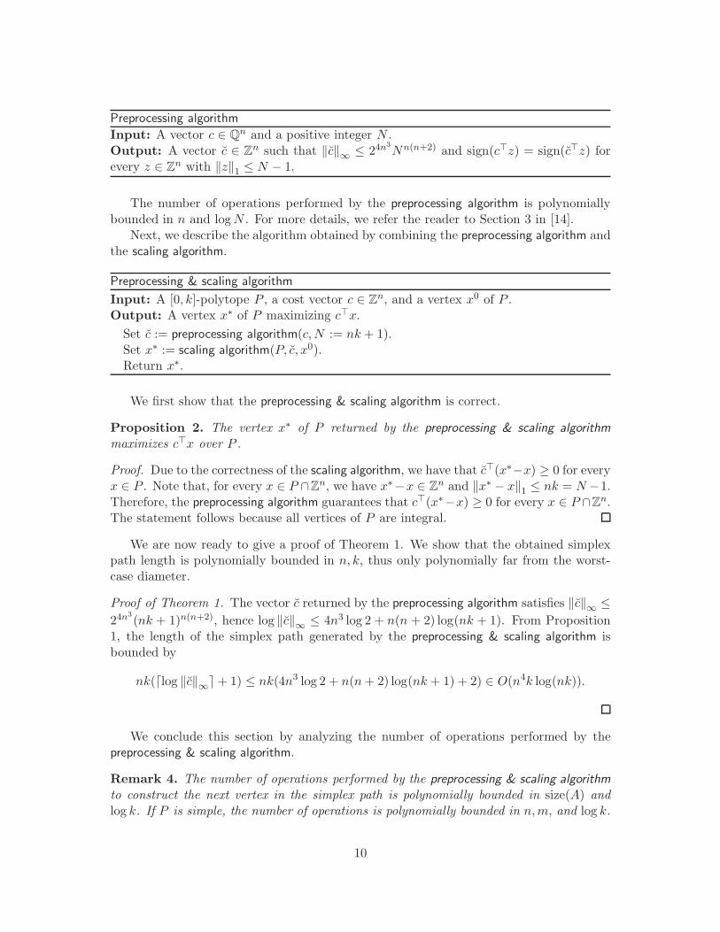
Preprocessing algorithm
Input: A vector c ∈ Qn and a positive integer N .Output: A vector c ∈ Zn such that ‖c‖∞ ≤ 24n
3Nn(n+2) and sign(c⊤z) = sign(c⊤z) for
every z ∈ Zn with ‖z‖1 ≤ N − 1.
The number of operations performed by the preprocessing algorithm is polynomiallybounded in n and logN . For more details, we refer the reader to Section 3 in [14].
Next, we describe the algorithm obtained by combining the preprocessing algorithm andthe scaling algorithm.
Preprocessing & scaling algorithm
Input: A [0, k]-polytope P , a cost vector c ∈ Zn, and a vertex x0 of P .Output: A vertex x∗ of P maximizing c⊤x.
Set c := preprocessing algorithm(c,N := nk + 1).Set x∗ := scaling algorithm(P, c, x0).Return x∗.
We first show that the preprocessing & scaling algorithm is correct.
Proposition 2. The vertex x∗ of P returned by the preprocessing & scaling algorithm
maximizes c⊤x over P .
Proof. Due to the correctness of the scaling algorithm, we have that c⊤(x∗−x) ≥ 0 for everyx ∈ P . Note that, for every x ∈ P ∩Zn, we have x∗−x ∈ Zn and ‖x∗ − x‖1 ≤ nk = N−1.Therefore, the preprocessing algorithm guarantees that c⊤(x∗−x) ≥ 0 for every x ∈ P ∩Zn.The statement follows because all vertices of P are integral.
We are now ready to give a proof of Theorem 1. We show that the obtained simplexpath length is polynomially bounded in n, k, thus only polynomially far from the worst-case diameter.
Proof of Theorem 1. The vector c returned by the preprocessing algorithm satisfies ‖c‖∞ ≤24n
3(nk + 1)n(n+2), hence log ‖c‖∞ ≤ 4n3 log 2 + n(n + 2) log(nk + 1). From Proposition
1, the length of the simplex path generated by the preprocessing & scaling algorithm isbounded by
nk(⌈log ‖c‖∞⌉+ 1) ≤ nk(4n3 log 2 + n(n+ 2) log(nk + 1) + 2) ∈ O(n4k log(nk)).
We conclude this section by analyzing the number of operations performed by thepreprocessing & scaling algorithm.
Remark 4. The number of operations performed by the preprocessing & scaling algorithm
to construct the next vertex in the simplex path is polynomially bounded in size(A) andlog k. If P is simple, the number of operations is polynomially bounded in n,m, and log k.
10

Proof. The number of operations performed by the preprocessing & scaling algorithm toconstruct the next vertex in the simplex path is the sum of: (i) the number of operationsneeded to compute c, and (ii) the number of operations performed by the scaling algorithm,with cost vector c, to construct the next vertex in the simplex path. The vector c can becomputed with a number of operations polynomially bounded in n and log(nk) [14]. FromRemark 3, (ii) is polynomially bounded in size(A) and log ‖c‖∞, and by O(n2m log2 ‖c‖∞)if P is simple. To conclude the proof, we only need to observe that log ‖c‖∞ is polynomiallybounded in n and log k.
4 The iterative algorithm
In this section, we design a simplex algorithm that yields simplex path whose lengthdepends on n, k, and α, where α denotes the largest absolute value of the entries of A. Wedefine [m] := 1, 2, . . . ,m and refer to the rows of A as ai, for i ∈ [m]. Next, we presentour iterative algorithm.
Iterative algorithm
Input: A [0, k]-polytope P , a cost vector c ∈ Zn, and a vertex x0 of P .Output: A vertex x∗ of P maximizing c⊤x.
0: Let E := ∅ and x∗ := x0.1: Let c be the projection of c onto the subspace x ∈ Rn | a⊤i x = 0 for i ∈ E of Rn. If
c = 0 return x∗, otherwise go to 2.
2: Let c ∈ Zn be defined by ci :=⌊
n3kα‖c‖∞
ci
⌋
for i = 1, . . . , n.
3: Consider the following pair of primal and dual LP problems:max c⊤xs.t. a⊤i x = bi i ∈ E
a⊤i x ≤ bi i ∈ [m] \ E(P )
min b⊤ys.t. A⊤y = c
yi ≥ 0 i ∈ [m] \ E .(D)
Use the scaling algorithm to compute an optimal vertex x of (P ) starting from x∗.Compute an optimal solution y to the dual (D) such that (i) y has at most n nonzerocomponents, and (ii) yj = 0 for every j ∈ [m] \ E such that aj can be written as alinear combination of ai, i ∈ E .Let H := i | yi > nk, and let h ∈ H \ E . Add the index h to the set E , set x∗ := x,and go back to step 1.
As the name suggests, the above algorithm is iterative in nature. In particular, aniteration of the algorithm corresponds to one execution of steps 1, 2, and 3.
4.1 Well-defined
In this section we prove that the iterative algorithm is well-defined, meaning that it canindeed perform all the instructions stated in its steps. First we show that, when theiterative algorithm calls the scaling algorithm in step 3, x∗ is a valid input.
11
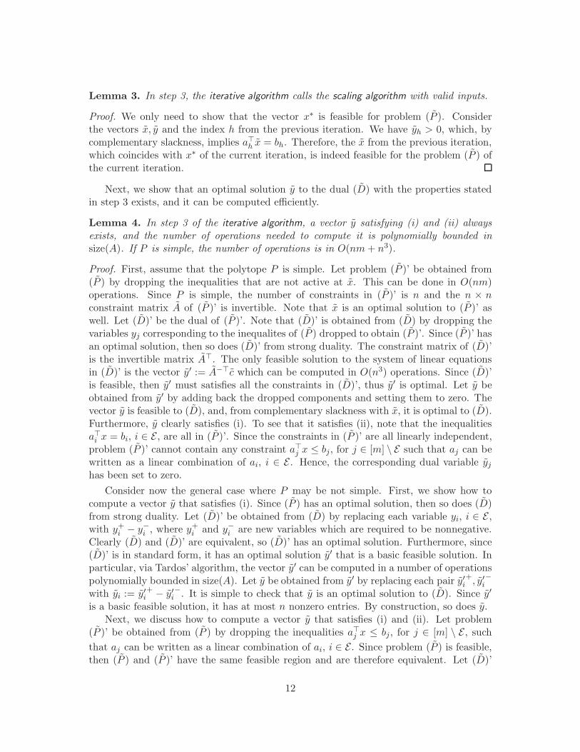
Lemma 3. In step 3, the iterative algorithm calls the scaling algorithm with valid inputs.
Proof. We only need to show that the vector x∗ is feasible for problem (P ). Considerthe vectors x, y and the index h from the previous iteration. We have yh > 0, which, bycomplementary slackness, implies a⊤h x = bh. Therefore, the x from the previous iteration,which coincides with x∗ of the current iteration, is indeed feasible for the problem (P ) ofthe current iteration.
Next, we show that an optimal solution y to the dual (D) with the properties statedin step 3 exists, and it can be computed efficiently.
Lemma 4. In step 3 of the iterative algorithm, a vector y satisfying (i) and (ii) alwaysexists, and the number of operations needed to compute it is polynomially bounded insize(A). If P is simple, the number of operations is in O(nm+ n3).
Proof. First, assume that the polytope P is simple. Let problem (P )’ be obtained from(P ) by dropping the inequalities that are not active at x. This can be done in O(nm)operations. Since P is simple, the number of constraints in (P )’ is n and the n × nconstraint matrix A of (P )’ is invertible. Note that x is an optimal solution to (P )’ aswell. Let (D)’ be the dual of (P )’. Note that (D)’ is obtained from (D) by dropping thevariables yj corresponding to the inequalites of (P ) dropped to obtain (P )’. Since (P )’ hasan optimal solution, then so does (D)’ from strong duality. The constraint matrix of (D)’is the invertible matrix A⊤. The only feasible solution to the system of linear equationsin (D)’ is the vector y′ := A−⊤c which can be computed in O(n3) operations. Since (D)’is feasible, then y′ must satisfies all the constraints in (D)’, thus y′ is optimal. Let y beobtained from y′ by adding back the dropped components and setting them to zero. Thevector y is feasible to (D), and, from complementary slackness with x, it is optimal to (D).Furthermore, y clearly satisfies (i). To see that it satisfies (ii), note that the inequalitiesa⊤i x = bi, i ∈ E , are all in (P )’. Since the constraints in (P )’ are all linearly independent,problem (P )’ cannot contain any constraint a⊤j x ≤ bj, for j ∈ [m] \ E such that aj can bewritten as a linear combination of ai, i ∈ E . Hence, the corresponding dual variable yjhas been set to zero.
Consider now the general case where P may be not simple. First, we show how tocompute a vector y that satisfies (i). Since (P ) has an optimal solution, then so does (D)from strong duality. Let (D)’ be obtained from (D) by replacing each variable yi, i ∈ E ,with y+i − y−i , where y+i and y−i are new variables which are required to be nonnegative.Clearly (D) and (D)’ are equivalent, so (D)’ has an optimal solution. Furthermore, since(D)’ is in standard form, it has an optimal solution y′ that is a basic feasible solution. Inparticular, via Tardos’ algorithm, the vector y′ can be computed in a number of operationspolynomially bounded in size(A). Let y be obtained from y′ by replacing each pair y′i
+, y′i−
with yi := y′i+ − y′i
−. It is simple to check that y is an optimal solution to (D). Since y′
is a basic feasible solution, it has at most n nonzero entries. By construction, so does y.Next, we discuss how to compute a vector y that satisfies (i) and (ii). Let problem
(P )’ be obtained from (P ) by dropping the inequalities a⊤j x ≤ bj, for j ∈ [m] \ E , suchthat aj can be written as a linear combination of ai, i ∈ E . Since problem (P ) is feasible,then (P ) and (P )’ have the same feasible region and are therefore equivalent. Let (D)’
12

be the dual of (P )’. Note that (D)’ is obtained from (D) by dropping the variables yjcorresponding to the inequalities of (P ) dropped to obtain (P )’. Note that (P )’ has thesame form of (P ), thus, from the the first part of the proof, we can compute a vector y′
optimal to (D)’ with at most n nonzero components. Furthermore, y′ can be computedin a number of operations polynomially bounded in size(A). Let y be obtained from y′ byadding back the dropped components and setting them to zero. The vector y is feasibleto (D), and, from complementary slackness with x, it is optimal to (D). Furthermore, ysatisfies (i) and (ii).
In the next lemma, we show that at step 3 we can always find an index h ∈ H \ E .
Lemma 5. In step 3 of the iterative algorithm, we have H\E 6= ∅. In particular, the indexh exists at each iteration.
Proof. Let c, c, x and y be the vectors computed at a generic iteration of the iterative
algorithm. Let c = n3kα‖c‖∞
c, and note that c = ⌊c⌋. Moreover, we have ‖c‖∞ = n3kα and,
since this number is integer, we also have ‖c‖∞ = n3kα.Let B = i ∈ 1, . . . ,m | yi 6= 0. From property (i) of the vector y we know |B| ≤ n.
From the constraints of (D) we obtain
c =∑
i∈[m]
aiyi =∑
i∈B
aiyi. (3)
Note that yj ≥ 0 for every j ∈ B \ E since y is feasible to (D). Hence to prove thislemma we only need to show that
|yj| > nk for some j ∈ B \ E . (4)
The proof of (4) is divided into two cases.
In the first case we assume B ∩ E = ∅. Thus, to prove (4), we only need to show that|yj| > nk for some j ∈ B. To obtain a contradiction, we suppose |yj | ≤ nk for every j ∈ B.From (3) we obtain
‖c‖∞ ≤∑
j∈B
‖aj yj‖∞ =∑
j∈B
(
|yj| ‖aj‖∞)
≤∑
j∈B
(nk · α) ≤ n2kα.
However, this contradicts the fact that ‖c‖∞ = n3kα. Thus |yj| > nk for some j ∈ B, and(4) holds. This concludes the proof in the first case.
In the second case we assume that B ∩E is nonempty. In particular, we have |B \ E| ≤n − 1. In order to derive a contradiction, suppose that (4) does not hold, i.e., |yj| ≤ nkfor every j ∈ B \ E . From (3) we obtain
c =∑
i∈B
aiyi =∑
i∈B∩E
aiyi +∑
j∈B\E
aj yj.
13
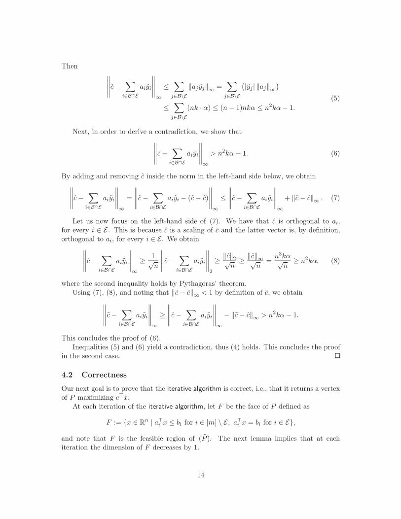
Then∥
∥
∥
∥
∥
c−∑
i∈B∩E
aiyi
∥
∥
∥
∥
∥
∞
≤∑
j∈B\E
‖aj yj‖∞ =∑
j∈B\E
(
|yj| ‖aj‖∞)
≤∑
j∈B\E
(nk · α) ≤ (n− 1)nkα ≤ n2kα− 1.
(5)
Next, in order to derive a contradiction, we show that
∥
∥
∥
∥
∥
c−∑
i∈B∩E
aiyi
∥
∥
∥
∥
∥
∞
> n2kα− 1. (6)
By adding and removing c inside the norm in the left-hand side below, we obtain
∥
∥
∥
∥
∥
c−∑
i∈B∩E
aiyi
∥
∥
∥
∥
∥
∞
=
∥
∥
∥
∥
∥
c−∑
i∈B∩E
aiyi − (c− c)
∥
∥
∥
∥
∥
∞
≤∥
∥
∥
∥
∥
c−∑
i∈B∩E
aiyi
∥
∥
∥
∥
∥
∞
+ ‖c− c‖∞ . (7)
Let us now focus on the left-hand side of (7). We have that c is orthogonal to ai,for every i ∈ E . This is because c is a scaling of c and the latter vector is, by definition,orthogonal to ai, for every i ∈ E . We obtain
∥
∥
∥
∥
∥
c−∑
i∈B∩E
aiyi
∥
∥
∥
∥
∥
∞
≥ 1√n
∥
∥
∥
∥
∥
c−∑
i∈B∩E
aiyi
∥
∥
∥
∥
∥
2
≥ ‖c‖2√n
≥ ‖c‖∞√n
=n3kα√
n≥ n2kα, (8)
where the second inequality holds by Pythagoras’ theorem.Using (7), (8), and noting that ‖c− c‖∞ < 1 by definition of c, we obtain
∥
∥
∥
∥
∥
c−∑
i∈B∩E
aiyi
∥
∥
∥
∥
∥
∞
≥∥
∥
∥
∥
∥
c−∑
i∈B∩E
aiyi
∥
∥
∥
∥
∥
∞
− ‖c− c‖∞ > n2kα− 1.
This concludes the proof of (6).Inequalities (5) and (6) yield a contradiction, thus (4) holds. This concludes the proof
in the second case.
4.2 Correctness
Our next goal is to prove that the iterative algorithm is correct, i.e., that it returns a vertexof P maximizing c⊤x.
At each iteration of the iterative algorithm, let F be the face of P defined as
F := x ∈ Rn | a⊤i x ≤ bi for i ∈ [m] \ E , a⊤i x = bi for i ∈ E,
and note that F is the feasible region of (P ). The next lemma implies that at eachiteration the dimension of F decreases by 1.
14

Lemma 6. At each iteration, the row submatrix of A indexed by E has full row rank.Furthermore, at each iteration, its number of rows increases by exactly one.
Proof. We prove this lemma recursively. Clearly, the statement holds at the beginning ofthe algorithm because we have E = ∅.
Assume now that, at a general iteration, the row submatrix of A indexed by E hasfull row rank. From Lemma 5, the index h ∈ H \ E defined in step 3 of the algorithmexists. In particular, yh > nk. From property (ii) of the vector y, we have that ah islinearly independent from the vectors ai, i ∈ E . Hence the rank of the row submatrix ofA indexed by E ∪ h is one more than the rank of the row submatrix of A indexed by E .In particular, it has full row rank.
In the next three lemmas, we will prove that, at each iteration, every optimal solutionto (1) lies in F . Note that, since F is a face of P , it is also a [0, k]-polytope.
Suppose that an optimal solution y of (D) is known. The complementary slacknessconditions for linear programming imply that, for every x optimal for (P ), we have
yi > 0 ⇒ a⊤i x = bi i ∈ [m] \ E . (9)
Thus, in order to solve (P ), we can restrict the feasible region of (P ) by setting the primalconstraints in (9) to equality.
Now, suppose that our goal is to solve a variant of (P ) where we replace the cost vectorc with another cost vector c. Denote by (P ) this new LP problem. Note that y mightnot even be feasible for the dual problem (D) associated to (P ). Can we, under suitableconditions, still use y to conclude that a primal constraint is satisfied with equality byeach optimal solution to (P )? We show that, if y is ‘close’ to being feasible for (D), thenfor each index i ∈ [m] \ E such that yi is sufficiently large, we have that the correspondingprimal constraint is active at every optimal solution to (P ). Thus, in order to solve (P ),we can restrict the feasible region of (P ) by setting these primal constraints to equality.
In the following, for u ∈ Rn we denote by |u| the vector whose entries are |ui|, i =1, . . . n.
Lemma 7. Let x ∈ F , c ∈ Rn, and y ∈ Rm be such that∣
∣
∣A⊤y − c
∣
∣
∣≤ 1 (10)
yi ≥ 0 i ∈ [m] \ E (11)
yi > 0 ⇒ a⊤i x = bi i ∈ [m] \ E . (12)
Then for any vector x ∈ F ∩ Zn with c⊤x ≥ c⊤x, we have
yi > nk ⇒ a⊤i x = bi i ∈ [m] \ E .
Proof. Let u := (x− x), and let u+, u− ∈ Rn+ be defined as follows. For j ∈ [n],
u+j :=
uj if uj ≥ 0
0 if uj < 0,u−j :=
0 if uj ≥ 0
−uj if uj < 0.
15

Clearly u = u+ − u− and |u| = u+ + u−. Since c⊤x ≥ c⊤x, we have c⊤u ≥ 0.We prove this lemma by contradiction. Suppose that there exists h ∈ [m]\E such that
yh > nk and a⊤h x 6= bh. Since x ∈ F and ah, x, bh are integral, we have a⊤h x ≤ bh − 1. Werewrite (10) as A⊤y − 1 ≤ c ≤ A⊤y + 1. Thus
c⊤u = c⊤u+ − c⊤u− ≤ (A⊤y + 1)⊤u+ − (A⊤y − 1)⊤u−
= (A⊤y)⊤(u+ − u−) + 1⊤(u+ + u−) = (A⊤y)⊤u+ 1⊤ |u| . (13)
We can upper bound 1⊤ |u| in (13) by observing that |uj | ≤ k for all j ∈ [n], since u is thedifference of two vectors in [0, k]n. Thus
1⊤ |u| ≤ nk. (14)
We now compute an upper bound for (A⊤y)⊤u = y⊤Au in (13).
y⊤Au = yha⊤h u+
∑
i∈E
yia⊤i u+
∑
i∈[m]\E, i 6=h
yia⊤i u
< −nk +∑
i∈E
yia⊤i u+
∑
i∈[m]\E, i 6=h
yia⊤i u (15)
= −nk +∑
i∈[m]\E, i 6=h
yia⊤i u (16)
≤ −nk +∑
i∈[m]\E, i 6=h, yi>0
yia⊤i u (17)
≤ −nk. (18)
To prove the strict inequality in (15) we show yha⊤h u < −nk. We have yh > nk > 0, thus
condition (12) implies a⊤h x = bh. Since a⊤h x ≤ bh − 1, we get a⊤h u = a⊤h x− a⊤h x ≤ −1. Wemultiply yh > nk by a⊤h u and obtain yh · a⊤h u < nk · a⊤h u ≤ −nk. Equality (16) followsfrom the fact that, for each i ∈ E we have a⊤i x = bi and a⊤i x = bi since both x and x arein F , thus a⊤i u = 0. Inequality (17) follows from (11). To see why inequality (18) holds,first note that, from condition (12), yi > 0 implies a⊤i x = bi. Furthermore, since x ∈ F ,we have a⊤i x ≤ bi. Hence we have a⊤i u ≤ 0 and so yia
⊤i u ≤ 0.
By combining (13), (14) and (18) we obtain c⊤u < 0. This is a contradiction since wehave previously seen that c⊤u ≥ 0.
For a vector w ∈ Zn and a polyhedron Q ⊆ Rn, we say that a vector is w-maximal inQ if it maximizes w⊤x over Q.
Lemma 8. The set H given at step 3 of the iterative algorithm is such that every vector xthat is c-maximal in F satisfies a⊤i x = bi for every i ∈ H.
Proof. Clearly, we just need to prove the lemma for every vertex x of F that maximizesc⊤x over F . In particular, x is a vertex of P and is therefore integral.
16

Define c ∈ Rn as ci :=n3kα‖c‖∞
ci for i = 1, . . . , n. At step 3, x is an optimal vertex of
(P ), and y is an optimal solution to the dual (D). We have:
∣
∣
∣A⊤y − c
∣
∣
∣≤ 1 (19)
yi ≥ 0 i ∈ [m] \ E . (20)
Constraints (20) are satisfied since y is feasible for (D). Condition (19) holds because∣
∣A⊤y − c∣
∣ = |c− c| = c − c < 1. Moreover, the complementary slackness conditions (9)
are satisfied by x and y, because they are optimal for (P ) and (D), respectively.Thus, A, b, c, x, y satisfy the hypotheses of Lemma 7. Since the vector x is c-maximal
in F and c is a scaling of c, the vector x is also c-maximal in F . Since x ∈ F , we havec⊤x ≥ c⊤x. Then Lemma 7 implies
yi > nk ⇒ a⊤i x = bi i ∈ [m] \ E ,
that is, a⊤i x = bi for all i ∈ H.
Lemma 9. The set E updated in step 3 of the iterative algorithm is such that every vectorx∗ that is c-maximal in P satisfies a⊤i x
∗ = bi for i ∈ E.
Proof. Consider a vector x∗ that is c-maximal in P . We prove this lemma recursively.Clearly, the statement is true at the beginning of the algorithm, when E = ∅.
Suppose now that the statement is true at the beginning of a general iteration. At thebeginning of step 3 we have that x∗ is c-maximal in F , thus it is also c-maximal in F .When we add an index h ∈ H \ E to E at the end of step 3, by Lemma 8 we obtain thata⊤h x
∗ = bh. Thus, at each iteration of the algorithm we have a⊤i x∗ = bi for i ∈ E .
In the next theorem, we show that the iterative algorithm is correct.
Theorem 3. The vector x∗ returned by the iterative algorithm is an optimal solution tothe LP problem (1).
Proof. Consider the iteration of the iterative algorithm when the vector x∗ is returned atstep 1. Let the set E be as defined in the algorithm when x∗ is returned. Up to reorderingthe inequalities defining P , we can assume, without loss of generality, that E = 1, . . . , r.Consider the following primal/dual pair:
max c⊤xs.t. a⊤i x = bi i = 1, . . . , r
a⊤i x ≤ bi i = r + 1, . . . ,m(P )
min b⊤ys.t. A⊤y = c
yi ≥ 0 i = r + 1, . . . ,m.(D)
Note that the feasible region of (P ) is the same of (P ), and it consists of the face Fof P obtained by setting to equality all the constraints indexed by E . Furthermore, theobjective function of (P ) coincides with the one of (1).
Let AE be the row submatrix of A indexed by E . By Lemma 6, the rank of AE is r.When, at step 1, we project c onto x ∈ Rn | AEx = 0, we get c = c−A⊤
E (AEA⊤E )
−1AEc.
17

Since the termination condition is triggered at this iteration, we have c = 0. This impliesc = A⊤
E z, where z := (AEA⊤E )
−1AEc.Let y ∈ Rm be defined by yi := zi for i = 1, . . . , r, and yi := 0 for i = r + 1, . . . ,m.
First, y is feasible for (D). In fact yi ≥ 0 for i = r + 1, . . . ,m and
A⊤y =
m∑
i=1
yiai =
r∑
i=1
ziai = A⊤E z = c.
In particular, x∗ is feasible for (P ). We have
c⊤x∗ = y⊤Ax∗ =m∑
i=1
yia⊤i x
∗ =r
∑
i=1
yia⊤i x
∗ =r
∑
i=1
yibi = y⊤b.
By strong duality, x∗ is c-maximal in F . If x∗ is not c-maximal in P , then there exista different vector x† that is c-maximal in P . In particular, we have c⊤x† > c⊤x∗. FromLemma 9, the vector x† lies in F . Since x∗ is c-maximal in F , we obtain c⊤x† ≤ c⊤x∗, acontradiction. This shows that x∗ is c-maximal in P .
4.3 Length of simplex path
We now present a proof of Theorem 2, which provides a bound on the length of the simplexpath generated by the iterative algorithm.
Proof of Theorem 2. First, note that the iterative algorithm constructs a simplex pathfrom x0 to the output vector. This is the path obtained by merging all the simplex pathsconstructed by the scaling algorithm in step 3 at each iteration. From Lemma 3, theiterative algorithm can indeed call the scaling algorithm with input vertex the current x∗,since x∗ is feasible for problem (P ).
Next, we upper bound the length of the generated simplex path. First, note that theiterative algorithm performs at most n iterations. This is because, by Lemma 6, at eachiteration the rank of the row submatrix of A indexed by E increases by one. Therefore, atiteration n+ 1, the subspace x ∈ Rn | a⊤i x = 0 for i ∈ E in step 1 is the origin. Hencethe projection c of c onto this subspace is the origin, and the algorithm terminates byreturning the current vector x∗.
Each time the iterative algorithm performs step 3, it calls the scaling algorithm withinput F , x∗, and c. Since F is a [0, k]-polytope, by Proposition 1, each time the scaling
algorithm is called, it generates a simplex path of length at most nk(⌈log ‖c‖∞⌉+1), where‖c‖∞ = n3kα. Since log ‖c‖∞ ∈ O(log(nkα)), each time we run the scaling algorithm,we generate a simplex path of length in O(nk log(nkα)). Therefore, the simplex pathgenerated throughout the entire algorithm has length in O(n2k log(nkα)).
We immediately obtain the following corollary of Theorem 2.
Corollary 1. If α is polynomially bounded in n, k, then the length of the simplex pathgenerated by the iterative algorithm is in O(n2k log(nk)). If we also assume k = 1, thelength reduces to O(n2 log n).
18
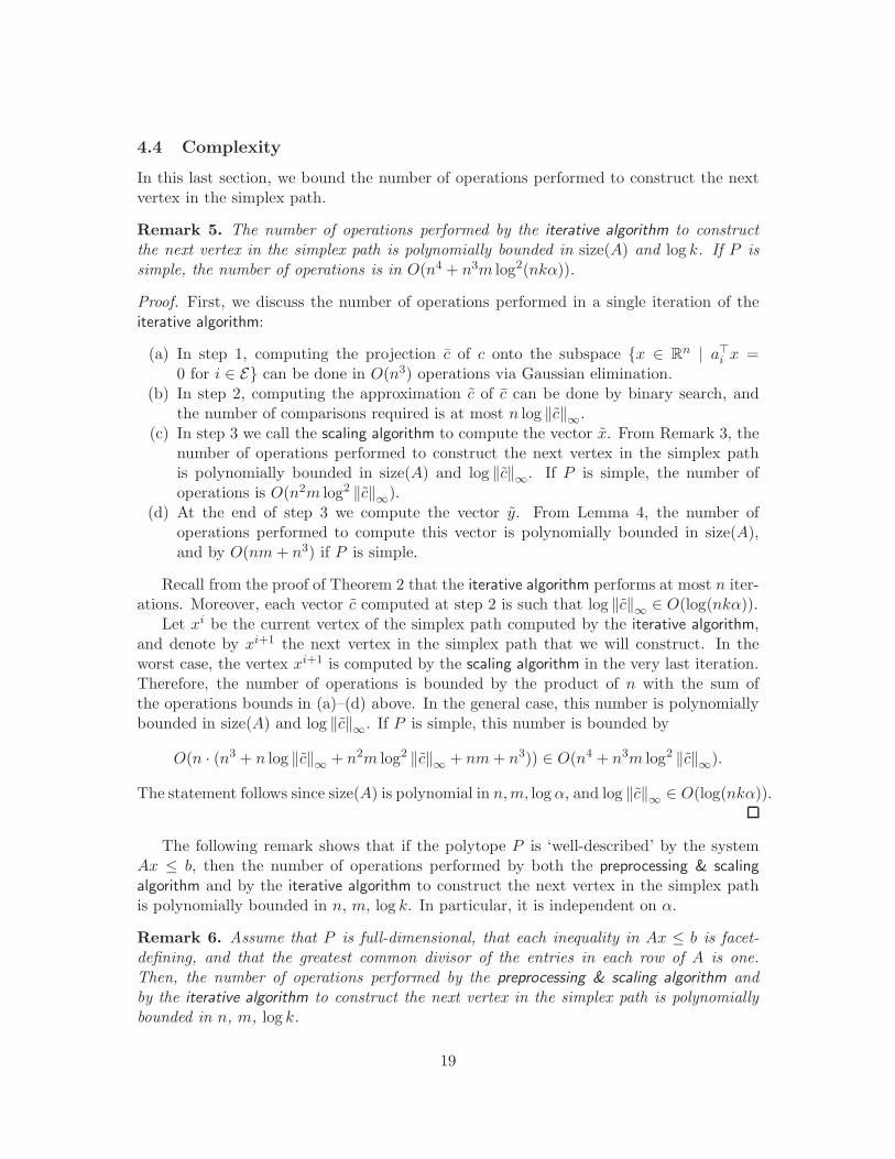
4.4 Complexity
In this last section, we bound the number of operations performed to construct the nextvertex in the simplex path.
Remark 5. The number of operations performed by the iterative algorithm to constructthe next vertex in the simplex path is polynomially bounded in size(A) and log k. If P issimple, the number of operations is in O(n4 + n3m log2(nkα)).
Proof. First, we discuss the number of operations performed in a single iteration of theiterative algorithm:
(a) In step 1, computing the projection c of c onto the subspace x ∈ Rn | a⊤i x =0 for i ∈ E can be done in O(n3) operations via Gaussian elimination.
(b) In step 2, computing the approximation c of c can be done by binary search, andthe number of comparisons required is at most n log ‖c‖∞.
(c) In step 3 we call the scaling algorithm to compute the vector x. From Remark 3, thenumber of operations performed to construct the next vertex in the simplex pathis polynomially bounded in size(A) and log ‖c‖∞. If P is simple, the number ofoperations is O(n2m log2 ‖c‖∞).
(d) At the end of step 3 we compute the vector y. From Lemma 4, the number ofoperations performed to compute this vector is polynomially bounded in size(A),and by O(nm+ n3) if P is simple.
Recall from the proof of Theorem 2 that the iterative algorithm performs at most n iter-ations. Moreover, each vector c computed at step 2 is such that log ‖c‖∞ ∈ O(log(nkα)).
Let xi be the current vertex of the simplex path computed by the iterative algorithm,and denote by xi+1 the next vertex in the simplex path that we will construct. In theworst case, the vertex xi+1 is computed by the scaling algorithm in the very last iteration.Therefore, the number of operations is bounded by the product of n with the sum ofthe operations bounds in (a)–(d) above. In the general case, this number is polynomiallybounded in size(A) and log ‖c‖∞. If P is simple, this number is bounded by
O(n · (n3 + n log ‖c‖∞ + n2m log2 ‖c‖∞ + nm+ n3)) ∈ O(n4 + n3m log2 ‖c‖∞).
The statement follows since size(A) is polynomial in n,m, log α, and log ‖c‖∞ ∈ O(log(nkα)).
The following remark shows that if the polytope P is ‘well-described’ by the systemAx ≤ b, then the number of operations performed by both the preprocessing & scaling
algorithm and by the iterative algorithm to construct the next vertex in the simplex pathis polynomially bounded in n, m, log k. In particular, it is independent on α.
Remark 6. Assume that P is full-dimensional, that each inequality in Ax ≤ b is facet-defining, and that the greatest common divisor of the entries in each row of A is one.Then, the number of operations performed by the preprocessing & scaling algorithm andby the iterative algorithm to construct the next vertex in the simplex path is polynomiallybounded in n, m, log k.
19

Proof. From Remark 4 and Remark 5, the number of operations performed by eitheralgorithm to construct the next vertex in the simplex path is polynomially bounded insize(A) and log k. Recall that size(A) is polynomial in n, m, and log α. Therefore, itsuffices to show that log α is polynomially bounded in n and log k.
Denote by ϕ the facet complexity of P and by ν the vertex complexity of P . FromTheorem 10.2 in [23], we know that ϕ and ν are polynomially related, and in particularϕ ≤ 4n2ν. Since P is a [0, k]-polytope, we have ν ≤ n log k. Due to the assumptions inthe statement of the remark, and Remark 1.1 in [7], we obtain that log α ≤ nϕ. Hence,log α ≤ nϕ ≤ 4n3ν ≤ 4n4 log k.
Note that the assumptions in Remark 6 are without loss of generality, and it is well-known that we can reduce ourselves to this setting in polynomial time. Remark 6 thenimplies that, if we assume that k is polynomially bounded by n and m, then both algo-rithms run in strongly polynomial time.
To conclude, we highlight that all the obtained bounds on the number of operationsperformed by our algorithms (see Remarks 1–6) also depend on the number m of inequali-ties in the system Ax ≤ b. This is in contrast with the lengths of the simplex paths, whichonly depend on n and k. This difference is to be expected, since in order to determine thenext vertex, the algorithm needs to read all the inequalities defining the polytope, thusthe number of operations must depend also on m.
References
[1] D. Acketa and J. Zunic. On the maximal number of edges of convex digital polygonsincluded into an m×m-grid. Journal of Combinatorial Theory, Series A, 69(2):358– 368, 1995.
[2] R.K. Ahuja, T.L. Magnanti, and J.B. Orlin. Network Flows: Theory, Algorithms,and Applications. Prentice Hall, Englewood Cliffs NJ, 1993.
[3] N. Alon and V.H. Vu. Anti-hadamard matrices, coin weighing, threshold gates, andindecomposable hypergraphs. Journal of Combinatorial Theory, Series A, 79:133–160, 1997.
[4] A. Balog and I. Barany. On the convex hull of the integer points in a disc. InProceedings of the seventh annual symposium on Computational geometry, SCG ’91,pages 162–165, New York, NY, USA, 1991. ACM.
[5] D. Bertsimas and J. Tsitsiklis. Introduction to Linear Optimization. Athena Scientific,Belmont, MA, 1997.
[6] M. Blanchard, J. De Loera, and Q. Louveaux. On the length of monotone paths inpolyhedra. arXiv:2001.09575, 2020.
[7] M. Conforti, G. Cornuejols, and G. Zambelli. Integer Programming. Springer, 2014.
20

[8] A. Del Pia and C. Michini. On the diameter of lattice polytopes. Discrete & Com-putational Geometry, 55(3):681–687, 2016.
[9] A. Deza, G. Manoussakis, and S. Onn. Primitive zonotopes. Discrete & Computa-tional Geometry, 60(1):27–39, July 2018.
[10] A. Deza and L. Pournin. Improved bounds on the diameter of lattice polytopes. ActaMathematica Hungarica, 154(2):457–469, 2018.
[11] A. Deza, L. Pournin, and N. Sukegawa. The diameter of lattice zonotopes. Proceedingsof the American Mathematical Society (to appear), 2020.
[12] E.A. Dinic. The method of scaling and transportation problems. Issled. Diskret. Mat.Science, Moscow. (In Russian.), 1973.
[13] J. Edmonds and R.M. Karp. Theoretical improvements in algorithmic efficiency fornetwork flow problems. Journal of the Association for Computing Machinery, 19:248–264, 1972.
[14] A. Frank and E Tardos. An application of simultaneous diophantine approximationin combinatorial optimization. Combinatorica, 7:49–65, 1987.
[15] H.N. Gabow. Scaling algorithms for network problems. Journal of Computer andSystemSciences, 31:148–168, 1985.
[16] T. Kitahara, T. Matsui, and S. Mizuno. On the number of solutions generatedby Dantzig’s simplex method for LP with bounded variables. Pacific Journal ofOptimization, 8(3):447–455, 7 2012.
[17] T. Kitahara and S. Mizuno. A bound for the number of different basic solutionsgenerated by the simplex method. Mathematical Programming, Series A, 137:579–586, 2013.
[18] P. Kleinschmidt and S. Onn. On the diameter of convex polytopes. Discrete Mathe-matics, 102:75–77, 1992.
[19] A.K. Lenstra, H.W. Lenstra, and L. Lovasz. Factoring polynomials with rationalcoefficients. Mathematische Annalen, 261:515–534, 1982.
[20] S. Mizuno. The simplex method using Tardos’ basic algorithm is strongly polynomialfor totally unimodular LP under nondegeneracy assumption. Optimization Methodsand Software, 31(6):1298–1304, 2016.
[21] S. Mizuno, N. Sukegawa, and A. Deza. An enhanced primal-simplex based Tardos’algorithm for linear optimization. Journal of the Operations Research Society ofJapan, 61(2):186–196, 2018.
[22] D.J. Naddef. The Hirsch conjecture is true for (0, 1)-polytopes. Mathematical Pro-gramming, 45:109–110, 1989.
21

[23] A. Schrijver. Theory of Linear and Integer Programming. Wiley, Chichester, 1986.
[24] A. Schrijver. Combinatorial Optimization. Polyhedra and Efficiency. Springer-Verlag,Berlin, 2003.
[25] A.S. Schulz, R. Weismantel, and G.M. Ziegler. 0/1-integer programming: Optimiza-tion and augmentation are equivalent. In Proceedings of ESA ’95, pages 473–483,1995.
[26] E. Tardos. A strongly polynomial algorithm to solve combinatorial linear programs.Operations Research, 34(2):250–256, 1986.
[27] T. Thiele. Extremalprobleme fur Punktmengen. Master’s thesis, Freie UniversitatBerlin, 1991.
[28] Gunter M. Ziegler. Lectures on 0/1-polytopes. In Gil Kalai and Gunter M. Ziegler,editors, Polytopes — Combinatorics and Computation, pages 1–41. Birkhauser Basel,Basel, 2000.
22