Shrinkage estimation and the use of additional information when calibrating in the presence of random effects

Research Article

Received 14 February 2012, Accepted 11 April 2013 Published online 23 May 2013 in Wiley Online Library

(wileyonlinelibrary.com) DOI: 10.1002/sim.5846

Shrinkage estimation and the use ofadditional information when calibratingin the presence of random effectsSamuel D. Oman*†

Let x denote a precise measurement of a quantity and Y an inexact measurement, which is, however, lessexpensive or more easily obtained than x. We have available a calibration set comprising clustered sets of .x; Y /observations, obtained from different sampling units. At the prediction step, we will only observe Y for a newunit, and we wish to estimate the corresponding unknown x, which we denote by �. This problem has beentreated under the assumption that x and Y are linearly related. Here, we expand on those results in threedirections: First, we show that if we center � about a known value c, for example, the mean x-value of thecalibration set, then the proposed estimator now shrinks to c. Second, we examine in detail the performanceof the estimator, which was proposed when one or more .x; Y / observations can be obtained for the newsubject. Third, we compare the Fieller-like confidence intervals, previously proposed, with t -like intervals basedon asymptotic moments of the point estimate. We illustrate and evaluate our procedures in the context of a dataset of true bladder-volumes (x) and ultrasound measurements (Y ). Copyright © 2013 John Wiley & Sons, Ltd.

Keywords: calibration; confidence intervals; mixed model; prediction; shrinkage

1. Introduction

Suppose the scalar variable x is a precise value of a quantity of interest and Y is an imprecise value,which is, however, cheaper or more easily obtained. We wish to use a calibration set, comprising mea-surements of both x and Y , to estimate the relation between the variables. At the future prediction step,only Y will be obtained, and we wish to estimate the corresponding unobserved x. If the calibration datamay be modeled by a simple linear regression

Yi D ˇ0C ˇ1xi C �i ; �i �ind N�0; �2

�; i D 1; : : : ; n;

and if

Y0 D ˇ0C ˇ1� C �0

denotes the new observation with � the fixed but unknown x, then clearly

Z � .Y0 � ˇ0/=ˇ1 �N��; �2=ˇ21

�: (1)

The classical estimator of � [1, 2] is then

OZ D�Y0 � O0

�= O1; (2)

Department of Statistics, Hebrew University, Mount Scopus, Jerusalem 91905, Israel*Correspondence to: Samuel D. Oman, Department of Statistics, Hebrew University, Mount Scopus, Jerusalem 91905, Israel.†E-mail: [email protected]

4090

Copyright © 2013 John Wiley & Sons, Ltd. Statist. Med. 2013, 32 4090–4101

S. D. OMAN

where Oi are the estimates of ˇi from the calibration set. Although OZ has no moments, being the ratioof two normal random variables, a 100.1� �/%-level confidence region for � is given by8<

:� W�Y0 � O0 � O1�

�2s2 Œ1C 1=nC .� � Nx/2=sxx�

6 F� .1; n� 1/

9>=>; ; (3)

where sxx D†niD1.xi � Nx/2, and Oi and s2 are the usual estimates of ˇi and �2 [3].

In many applications, however, the calibration data must be interpreted as clustered observationsobtained from different sampling units such as subjects, experiments or machines, while at the pre-diction step, we wish to estimate � for a new sampling unit. For example, we might want to estimateparticle-mass concentration � using a new machine, which gives an infrared thermal imaging measure-ment Y0, and have available a calibration set comprising sets of measurements Y , together with moreprecise measurements x obtained using filter weighing, for a number of machines of this type, which arealready in use. In the application in [4] discussed later, we wish to use a transvaginal ultrasound mea-surement Y0 to estimate a woman’s bladder-volume � , for example, before and after surgery for urinaryincontinence. At the calibration step, each of 23 different patients in a urodynamic clinic had up to eightknown volumes x induced by catheterization, and the corresponding ultrasound measurements Y wereobtained.

In such cases, subject-specific random effects need to be included at both the calibration and predic-tion steps. This was done in [5], where an analogue of the confidence regions in (3) was obtained and itsnumerical properties were studied. Regarding point estimation, a shrinkage estimator O� was proposed asan alternative to the analogue of OZ in (2). An estimator was also proposed for the case where additionalinformation, in the form of one or more .x; Y / observations, is available for the new subject, and wewant to utilize it to estimate future � values, without recomputing the calibration-step estimates. Thenumerical performance of these estimators was not, however, studied in depth.

Here, we first show that if � is centered about a particular x-value c (for example, the mean of thecalibration set or a value of � whose detection is particularly important), then O� now shrinks towardc, whereas the analogue to (2) does not. In the context of a data set of true bladder-volumes (x) andultrasound measurements (Y ), we show that centering substantially decreases the prediction error for �in a large region near c, at the expense of a minimal increase for points farther away. Second, in thecontext of additional information, we show that as little as one such .x; Y / observation can dramaticallydecrease the prediction error of the proposed estimator. Third, we compare one version of the Fieller-likeconfidence intervals, proposed in [5], with t -like intervals based on the asymptotic moments of the ana-logue of OZ in (2). We find that the Fieller-like intervals have the desired coverage probability, whereasthe somewhat shorter t -like intervals do not.

In the next section, we describe the theoretical framework. In Section 3, we numerically examine theperformance of the estimators in the context of the bladder ultrasound data, using both simulations andcross-validation. Section 4 contains some concluding remarks, and the Appendix gives computationaldetails of the simulations.

2. Framework

2.1. The model

For n subjects, assume the observations at the calibration step are given by

Yij D ˇ0C ˇ1xij C b0i C b1ixij C �ij ; i D 1; : : : ; n

j D 1; : : : ; mi ;(4)

where .b0i ; b1i /t D bi �ind N.0;ˆ/ and �ij �ind N�0; �2

�independently. Letting

Y0 D ˇ0C ˇ1� C b0C b1� C �0 (5)

denote the observation for the new subject at the prediction step, we have that

Y0 �N�ˇ0C ˇ1�; �

2C Œ1; ��ˆŒ1; ��t�

(6)


4091

S. D. OMAN

so that now

Z �Y0 � ˇ0

ˇ1�N.�;Q.�//; (7)

where

Q.�/D��2C Œ1; ��ˆŒ1; ��t

�=ˇ21 : (8)

Thus, in contrast to the case with simple linear regression, both the mean and variance of Y0 containinformation on � . In particular, the variance of Z in (8) is now larger than in (1), and defining OZ as in

(2), where now O �N.ˇ;V/ is the mixed-model estimate of ˇ from the calibration data, does not utilizethis information. This suggests [5] the estimate

O� DOZ2

OZ2C OQ�OZ� OZ; (9)

where

OQ.�/DhO�2C .1; �/

�O C OV

�.1; �/t

i= O21 : (10)

This is motivated by the fact that if one knew the model parameters, and wished to minimizeE.�Z��/2

over � , the resulting estimator would be

Q� D�2

�2CQ.�/Z: (11)

2.2. Centering

Now suppose that in (5) we center � about a known value c, giving

Y0 D .ˇ0C ˇ1c/ C ˇ1.� � c/ C .b0C b1c/ C b1.� � c/ C �0

D ˛0 C ˛1�� C a0 C a1�

� C �0;

where �� D � � c and now .a0; a1/t � N

�0;ˆ�

�for ˆ� D GˆGt with G D

�1 c

0 1

�. Assume for

the moment that the model parameters are known. If we estimate �� by Z� defined as in (7), but using ˛instead of ˇ, it is immediate that the corresponding estimate of � , cCZ�, reduces to Z. Thus, centeringhas no effect when the simple estimator Z is used. However, if we estimate �� using the analogue to(11) (where now Q� is defined using ˆ� and ˛1), we obtain the following estimate of �:

Q�c D cC.��/2

.��/2CQ�.��/Z�

D cC.� � c/2

.� � c/2CQ.�/.Z � c/I (12)

here, we have used the fact that Q�.��/ D Q.�/. Thus, centering gives an estimator that contracts Ztoward c. As with (7) and (11), replacing the unknown parameters in (12) by their estimates gives theestimator

O�c D cC

�OZ � c

�2�OZ � c

�2C OQ

�OZ� � OZ � c� : (13)

This is the empirical Bayes estimator that would arise if we were to assume OZ j � �N��; OQ.�/

�and

� �N�c; �2

�and then estimate OQ.�/ by OQ

�OZ�

and �2 by�OZ � c

�2. However, one does not require a

4092


S. D. OMAN

Bayesian framework to use (13): the amount of shrinkage does not depend on a prior variance that must

be specified, but rather on the relationship of the distance between OZ and c, to the estimated variance

of OZ. Moreover, the shrinkage target c is not a prior mean for � , but rather a value for which we wishto obtain more precise estimates. For example, it might be a level of particle-mass concentration thatit is important not to exceed. In the context of bladder-volume ultrasound measurements, c might bethe mean or mode of the �-values obtained so far. We might update c periodically, as we obtain moreinformation on the population in question, but it is important to note that c cannot depend on Y0 forthe new subject being analyzed. The specification of c is somewhat similar in spirit to [6] where, in thecontext of estimating the random effect bi of subject i in the model Yij D �C bi C �ij (under the usualassumptions), estimators are considered of the form a NYi:Cc, where a and c are chosen with the objectiveof obtaining lower prediction error over a specified range of possible bi values .

2.3. Using additional information

Suppose it is possible to obtain a small number m0 > 1 of x measurements, together with the corre-sponding Y values, for the new subject, and we need to decide if it is worth doing this in order to helppredict future � values. For example, it might be possible (albeit expensive) to perform a short calibra-tion run on the new particle-mass measuring machine, before putting it into routine use. In the contextof the bladder-volume problem, if a new patient requires continuous monitoring of her bladder volumes,we might consider subjecting her to the invasive procedure needed to obtain some exact measurements,provided they would help when using ultrasound to estimate her future volumes.

Denoting the vectors of these measurements by x1 and y1, one approach would be to incorporate theminto the calibration set and recompute the parameter estimates. The prediction step would then be for asubject in the calibration set, putting us in the framework considered in [7–10], among others.

However, for practical reasons, it might not be feasible to refit the mixed model for each new subject.We then need a simple means to update the calibration-step estimates using .x1; y1/. This was done in[5]. Assume for the moment that the mixed-model parameters are known. Then, y1 is ancillary for � , andanalogous to (6), we now have

Y0 j y1 �N�N0C N1�; �

2C Œ1; ��‰ Œ1; ��t�

(14)

for N a suitably weighted average of ˇ and a vector ˇ� for the new subject, and

‰ Dˆ �ˆUt��2ICUˆUt

��1Uˆ (15)

with U D Œ1; x1�. If m0 > 2, then ˇ� D�UtU

��1Uty1 is simply an estimate of the coefficients of a

subject-specific regression line. If m0 D 1, then ˇ�0 is the intercept of a line with population slope ˇ1,which passes through .x1; y1/, whereas ˇ�1 is the slope of a line with population intercept ˇ0, whichpasses through the same point. Thus, we may define Z and Q�c as in (7), (11) and (8) but with N and ‰replacing ˇ and ˆ. Replacing the unknown parameters by their estimates gives the analogues to (2) and(13).

Note that these results depend crucially on the assumption that prediction is for a new subject, notin the calibration set. For, if the new Y0 is for subject i in the calibration set, then conditional on thecalibration data, Y0 has a

N�hˇ0C Ob0i

iChˇ1C Ob1i

i�; �2

�distribution. Thus, as opposed to (14), � no longer affects the variance of the relevant distribution throughthe quadratic form .1; �/‰.1; �/t .

2.4. Confidence intervals

In the case of simple linear regression, the region (3) is based on the facts that

Y0 � O0 � O1� �N�0; �2

h1C 1=nC .� � Nx/2 =sxx

i�(16)

and s2 � 2.n� 1/ independently. The region has exact coverage probability and comprises an intervalexactly when O1 is significant at the 1 � � level (which one would expect to occur in most realis-tic calibration scenarios); otherwise, (3) will define either two disjoint intervals or the whole real line


4093

S. D. OMAN

[11, p. 25ff]. An alternative approach is based on the asymptotic distribution of OZ [12]. Using the deltamethod, one has for large n that

OZ �N��;��2=ˇ21

h1C 1=nC .� � Nx/2 =sxx

i�; (17)

leading to the approximate .1� �/-level interval

OZ˙ t�=2.n� 1/�s=ˇO1

ˇ� 1C 1=nC

�OZ � Nx

�2=sxx

�1=2(18)

or, ignoring terms of O.1=n/,

OZ˙ t�=2.n� 1/�s=ˇO1

ˇ�I (19)

here, t�=2.n�1/ denotes the appropriate critical point from the t .n�1/ distribution. The Fieller interval(3), being exact, is generally preferred [2] to the t -like interval (18).

In the present context, the analogy to (16) is

Y0 � O0 � O1� �N�0; �2C .1; �/H.1; �/t

�; (20)

where HDˆCV, which led [5] to proposing the region8<:� W

�Y0 � O0 � O1�

�2O�2C .1; �/ OH.1; �/t

6 c�

9>=>; (21)

for an appropriate critical point c� . Analogous to (3), (21) gives a finite interval exactly whenO21=�O22C Ov22

�D O21=

hcvar.b1/Ccvar�O1

�i> c� . The value c� D F� .1; n � 1/ was suggested, to

account for the fact that OH reflects both variation within and between the n sampling units. The resultingintervals compared favorably with those obtained using bootstrap estimates of c� .

Because the Fieller-like region (21) no longer has exact coverage probability, being based on the

asymptotic distribution of O; O and OV, there is room to compare it with intervals analogous to (18).Instead of (17), we now have

OZ �N��;��2C .1; �/H.1; �/t

=ˇ21

�(22)

for large n, suggesting the interval

OZ˙ht�=2.n� 1/=

ˇO1

ˇi O�2C

�1; OZ

�OH�1; OZ

�t�1=2: (23)

Note that in the case of simple linear regression, (18) simplifies to (19) when O.1=n/ terms are ignoredin the asymptotic variance of OZ in (17). For our model, however, ignoring such terms in (20) only reducesH to ˆ, so we still need to estimate � by OZ in the asymptotic standard deviation in (23). It would be ofinterest to consider a t -like interval centered about O�, but we cannot do this as (9) leads to an asymptoticdistribution, which is asymmetric and depends on � in a very complicated way.

Finally, we note that centering � about c does not affect any of these intervals. For example, using thenotation of Section 2.2, we may replace (20) by

Y0 � O0 � O1�� N

�0; �2C .1; ��/H�.1; ��/t

�;

where H� D ˆ� C V�, and V� denotes the asymptotic covariance matrix of O . If we then construct aFieller-like interval for ��, it is immediate that this reduces to the interval (21) for � . Similar remarksapply to (23).

4094


S. D. OMAN

3. Numerical performance

3.1. An example

Figure 1(a) graphs the bladder-volume data described in Section 1, following the transformation andrescaling suggested in [11] and [5]. Table I gives the restricted maximum likelihood estimates andasymptotic confidence intervals (from the R function lme) for the parameters ˇ, ˆ and �2. Figure 2shows the estimates obtained using OZ and O�c , for several values of c, together with the approximateFieller and t -like confidence intervals. Intersecting a horizontal line through a particular value of Y0with one of the curves, and then projecting onto the � axis, gives the corresponding point estimate orconfidence limit.

0 5 10 15

050

010

0015

00

(a)

Induced bladder volume (cl)

Ultr

asou

nd v

olum

e (c

ubic

mm

)

0 5 10 15

05

1015

(b)

MS

E

Figure 1. (a) Ultrasound bladder volume versus induced bladder volume for 23 women. (b) Idealized meansquared error (MSE) (24) of Z and Q�c for several values of c.

Table I. Restricted maximum likelihood parameter estimates and approximate 95%confidence intervals (�D 12=

p1122).

Parameter Estimate Lower limit Upper limit

ˇ0 �54:479 �76:946 �32:011

ˇ1 69.192 63.319 75.065p11 37.945 20.924 68.812p22 13.582 9.632 19.153

� 0.318 �0:388 0.789� 54.017 47.614 61.282

0 5 10 15 20 25

050

010

0015

00

(a)

Y0

Y0

0 5 10 15 20 25

050

010

0015

00

(b)

Fiellert-like

Figure 2. (a) Point estimates using several methods. (b) Confidence intervals using two methods.


4095

S. D. OMAN

Observe first that O�0 is very similar to OZ. The motivation for O�0, as discussed preceding (11), was thatcontracting OZ toward 0 would lower its variance. However, in an empirical Bayes context, for our appli-cation (and presumably for many others as well), 0 is not a very realistic target value for � . Thus, OZ is

far from 0, the ‘estimated prior variance’�OZ � c

�2of � in (13) is large, and O�0 gives minimal shrinkage

toward 0.In contrast, both O�7 and O�10 have more realistic target values c and thus result in more shrink-

age. For example, we have 10:0 cl 6 O�10 6 10:2 cl when the corresponding estimates using OZ are10:0 cl 6 OZ 6 11:2 cl, and as OZ increases to 17:5 cl, the amount of shrinkage of O�10 increases to 1:5 cl.For values of OZ less than 10:0 cl, O�10 pulls the estimate upward toward 10:0 cl by increasing amountsuntil OZ reaches 8:0 cl (corresponding to O�10 D 9:0 cl); the amount of expansion then decreases to 0:2 clwhen OZ D 2:5 cl. Because O�10 and OZ differ over such a wide range of the �-axis, it is reasonable toexpect that their prediction accuracies will differ as well. Similar remarks apply to O�7.

Regarding the confidence intervals, for a given value of Y0, the distance between the approximateFieller and t -like upper limits is a bit larger than the distance between their lower limits, so that theFieller intervals are somewhat wider. For example, when Y0 D 500 mm3 (corresponding to OZ D 8:0 cl),the Fieller interval is .4:9 cl; 14:8 cl/ and the t -like interval is .3:8 cl; 12:2 cl/.

3.2. Point estimation

We now examine the accuracy of the estimators in Section 2.2, taking the values in Table I to be the trueparameter values. If it were possible to use Z and Q�c defined by (7) and (12), then a simple calculationshows that Q�c has bias

Q.�/.c � �/

.� � c/2CQ.�/

and standard deviation

.� � c/2

.� � c/2CQ.�/Q.�/1=2;

giving the idealized mean squared error (MSE)

MSE. Q�c ; �/D.� � c/2

.� � c/2CQ.�/Q.�/; (24)

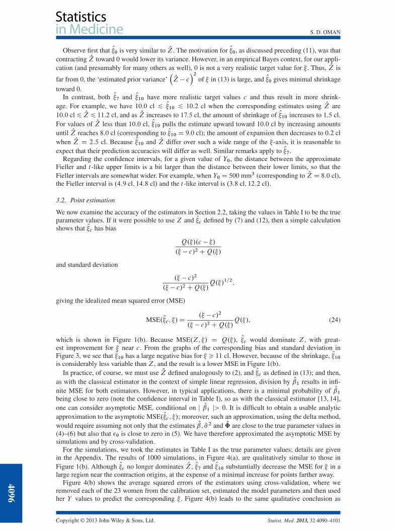
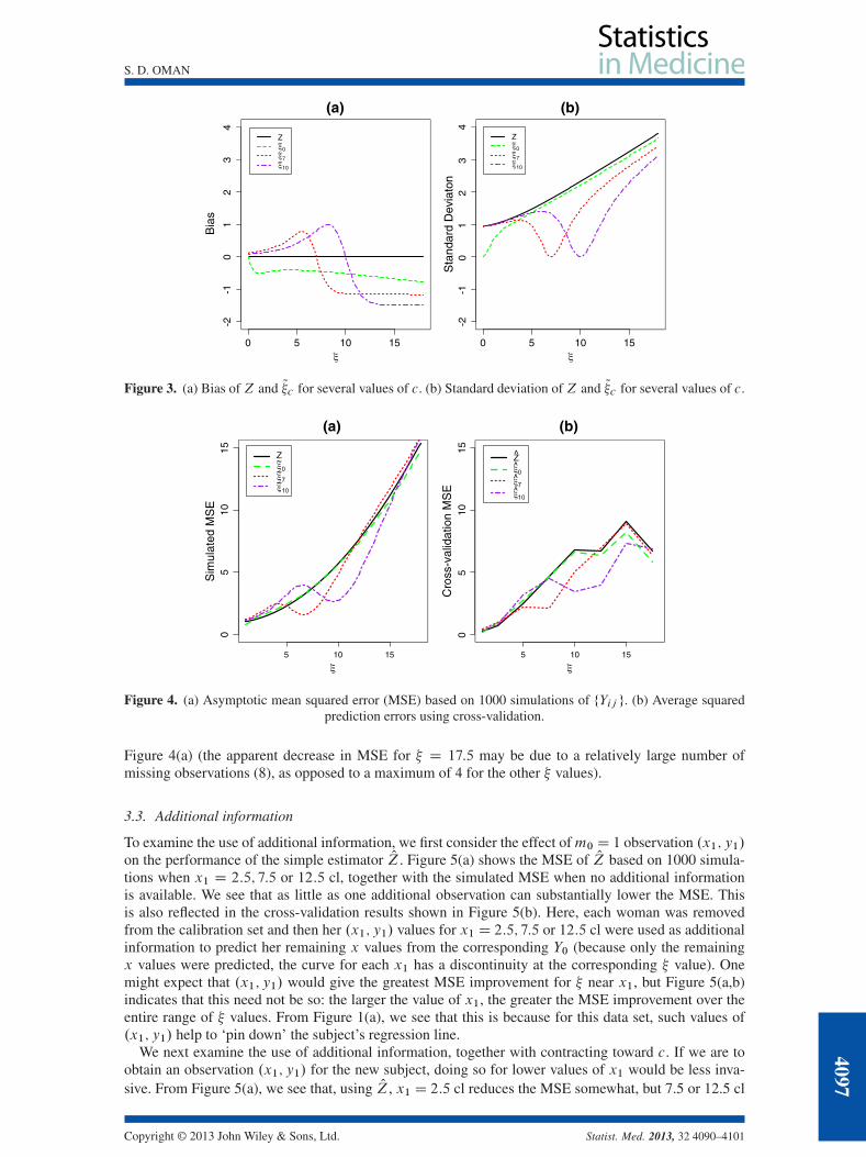
which is shown in Figure 1(b). Because MSE.Z; �/ D Q.�/, Q�c would dominate Z, with great-est improvement for � near c. From the graphs of the corresponding bias and standard deviation inFigure 3, we see that Q�10 has a large negative bias for � > 11 cl. However, because of the shrinkage, Q�10is considerably less variable than Z, and the result is a lower MSE in Figure 1(b).

In practice, of course, we must use OZ defined analogously to (2), and O�c as defined in (13); and then,as with the classical estimator in the context of simple linear regression, division by O1 results in infi-nite MSE for both estimators. However, in typical applications, there is a minimal probability of O1being close to zero (note the confidence interval in Table I), so as with the classical estimator [13, 14],one can consider asymptotic MSE, conditional on j O1 j> 0. It is difficult to obtain a usable analyticapproximation to the asymptotic MSE. O�c ; �/; moreover, such an approximation, using the delta method,would require assuming not only that the estimates O; O�2 and O are close to the true parameter values in(4)–(6) but also that �0 is close to zero in (5). We have therefore approximated the asymptotic MSE bysimulations and by cross-validation.

For the simulations, we took the estimates in Table I as the true parameter values; details are givenin the Appendix. The results of 1000 simulations, in Figure 4(a), are qualitatively similar to those inFigure 1(b). Although O�c no longer dominates OZ, O�7 and O�10 substantially decrease the MSE for � in alarge region near the contraction origins, at the expense of a minimal increase for points farther away.

Figure 4(b) shows the average squared errors of the estimators using cross-validation, where weremoved each of the 23 women from the calibration set, estimated the model parameters and then usedher Y values to predict the corresponding � . Figure 4(b) leads to the same qualitative conclusion as

4096


S. D. OMAN

0 5 10 15

-2-1

01

23

4

(a)

Bia

s

Z~~~

0 5 10 15

-2-1

01

23

4

(b)

Sta

ndar

d D

evia

ton

Z~~~

Figure 3. (a) Bias of Z and Q�c for several values of c. (b) Standard deviation of Z and Q�c for several values of c.

5 10 15

05

1015

(a)

Sim

ulat

ed M

SE

5 10 15

05

1015

(b)C

ross

-val

idat

ion

MS

E

Figure 4. (a) Asymptotic mean squared error (MSE) based on 1000 simulations of fYij g. (b) Average squaredprediction errors using cross-validation.

Figure 4(a) (the apparent decrease in MSE for � D 17:5 may be due to a relatively large number ofmissing observations (8), as opposed to a maximum of 4 for the other � values).

3.3. Additional information

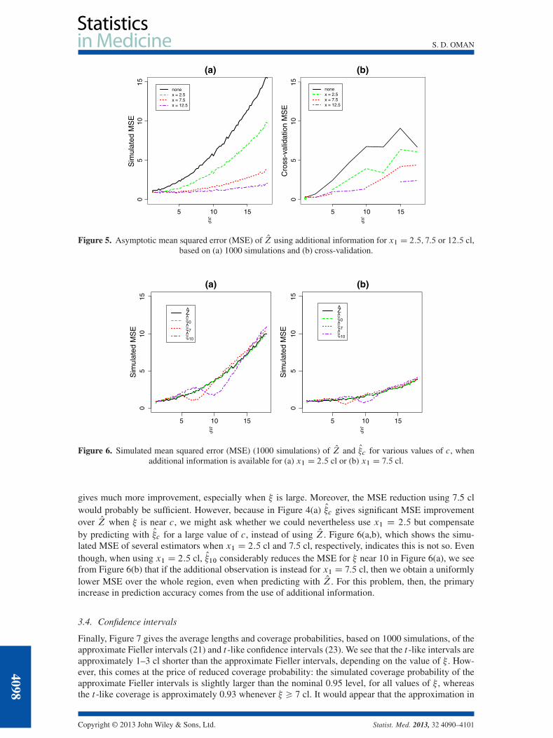
To examine the use of additional information, we first consider the effect ofm0 D 1 observation .x1; y1/on the performance of the simple estimator OZ. Figure 5(a) shows the MSE of OZ based on 1000 simula-tions when x1 D 2:5; 7:5 or 12:5 cl, together with the simulated MSE when no additional informationis available. We see that as little as one additional observation can substantially lower the MSE. Thisis also reflected in the cross-validation results shown in Figure 5(b). Here, each woman was removedfrom the calibration set and then her .x1; y1/ values for x1 D 2:5; 7:5 or 12:5 cl were used as additionalinformation to predict her remaining x values from the corresponding Y0 (because only the remainingx values were predicted, the curve for each x1 has a discontinuity at the corresponding � value). Onemight expect that .x1; y1/ would give the greatest MSE improvement for � near x1, but Figure 5(a,b)indicates that this need not be so: the larger the value of x1, the greater the MSE improvement over theentire range of � values. From Figure 1(a), we see that this is because for this data set, such values of.x1; y1/ help to ‘pin down’ the subject’s regression line.

We next examine the use of additional information, together with contracting toward c. If we are toobtain an observation .x1; y1/ for the new subject, doing so for lower values of x1 would be less inva-sive. From Figure 5(a), we see that, using OZ, x1 D 2:5 cl reduces the MSE somewhat, but 7.5 or 12.5 cl


4097

S. D. OMAN

5 10 15

05

1015

(a)

Sim

ulat

ed M

SE

nonex = 2.5x = 7.5x = 12.5

5 10 15

05

1015

(b)

Cro

ss-v

alid

atio

n M

SE

nonex = 2.5x = 7.5x = 12.5

Figure 5. Asymptotic mean squared error (MSE) of OZ using additional information for x1 D 2:5; 7:5 or 12:5 cl,based on (a) 1000 simulations and (b) cross-validation.

5 10 15

05

1015

(a)

Sim

ulat

ed M

SE

5 10 15

05

1015

(b)S

imul

ated

MS

E

Figure 6. Simulated mean squared error (MSE) (1000 simulations) of OZ and O�c for various values of c, whenadditional information is available for (a) x1 D 2:5 cl or (b) x1 D 7:5 cl.

gives much more improvement, especially when � is large. Moreover, the MSE reduction using 7.5 clwould probably be sufficient. However, because in Figure 4(a) O�c gives significant MSE improvementover OZ when � is near c, we might ask whether we could nevertheless use x1 D 2:5 but compensateby predicting with O�c for a large value of c, instead of using OZ. Figure 6(a,b), which shows the simu-lated MSE of several estimators when x1 D 2:5 cl and 7:5 cl, respectively, indicates this is not so. Eventhough, when using x1 D 2:5 cl, O�10 considerably reduces the MSE for � near 10 in Figure 6(a), we seefrom Figure 6(b) that if the additional observation is instead for x1 D 7:5 cl, then we obtain a uniformlylower MSE over the whole region, even when predicting with OZ. For this problem, then, the primaryincrease in prediction accuracy comes from the use of additional information.

3.4. Confidence intervals

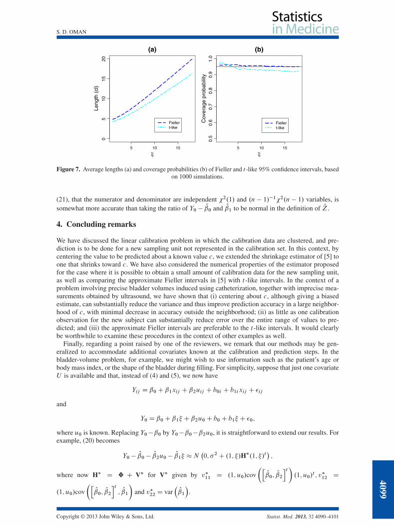
Finally, Figure 7 gives the average lengths and coverage probabilities, based on 1000 simulations, of theapproximate Fieller intervals (21) and t -like confidence intervals (23). We see that the t -like intervals areapproximately 1–3 cl shorter than the approximate Fieller intervals, depending on the value of � . How-ever, this comes at the price of reduced coverage probability: the simulated coverage probability of theapproximate Fieller intervals is slightly larger than the nominal 0.95 level, for all values of � , whereasthe t -like coverage is approximately 0.93 whenever � > 7 cl. It would appear that the approximation in

4098


S. D. OMAN

5 10 15

05

1015

20

(a)

Leng

th (

cl)

Fiellert-like

5 10 15

0.5

0.6

0.7

0.8

0.9

1.0

(b)

Cov

erag

e pr

obab

ility

Fiellert-like

Figure 7. Average lengths (a) and coverage probabilities (b) of Fieller and t-like 95% confidence intervals, basedon 1000 simulations.

(21), that the numerator and denominator are independent 2.1/ and .n � 1/�12.n � 1/ variables, issomewhat more accurate than taking the ratio of Y0 � O0 and O1 to be normal in the definition of OZ.

4. Concluding remarks

We have discussed the linear calibration problem in which the calibration data are clustered, and pre-diction is to be done for a new sampling unit not represented in the calibration set. In this context, bycentering the value to be predicted about a known value c, we extended the shrinkage estimator of [5] toone that shrinks toward c. We have also considered the numerical properties of the estimator proposedfor the case where it is possible to obtain a small amount of calibration data for the new sampling unit,as well as comparing the approximate Fieller intervals in [5] with t -like intervals. In the context of aproblem involving precise bladder volumes induced using catheterization, together with imprecise mea-surements obtained by ultrasound, we have shown that (i) centering about c, although giving a biasedestimate, can substantially reduce the variance and thus improve prediction accuracy in a large neighbor-hood of c, with minimal decrease in accuracy outside the neighborhood; (ii) as little as one calibrationobservation for the new subject can substantially reduce error over the entire range of values to pre-dicted; and (iii) the approximate Fieller intervals are preferable to the t -like intervals. It would clearlybe worthwhile to examine these procedures in the context of other examples as well.

Finally, regarding a point raised by one of the reviewers, we remark that our methods may be gen-eralized to accommodate additional covariates known at the calibration and prediction steps. In thebladder-volume problem, for example, we might wish to use information such as the patient’s age orbody mass index, or the shape of the bladder during filling. For simplicity, suppose that just one covariateU is available and that, instead of (4) and (5), we now have

Yij D ˇ0C ˇ1xij C ˇ2uij C b0i C b1ixij C �ij

and

Y0 D ˇ0C ˇ1� C ˇ2u0C b0C b1� C �0;

where u0 is known. Replacing Y0�ˇ0 by Y0�ˇ0�ˇ2u0, it is straightforward to extend our results. Forexample, (20) becomes

Y0 � O0 � O2u0 � O1� �N�0; �2C .1; �/H�.1; �/t

�;

where now H� D ˆ C V� for V� given by v�11 D .1; u0/cov

�hO0; O2

it�.1; u0/

t ; v�12 D

.1; u0/cov

�hO0; O2

it; O1

�and v�22 D var

�O1

�.


4099

S. D. OMAN

Appendix: Computational details

Let � D�ˇt ; �2; 11; 12; 22

�tdenote the parameters of the model (4). For given � and � , we may

write the asymptotic MSE discussed in Section 3.2 as

MSEasy.�; �/DEhg�O�; �0I �; �

�i; (25)

where the definition of the function g depends on the estimator being considered. Although g is anexplicitly defined, relatively simple function, (25) does not have a closed-form expression, and evaluationby numerical integration is problematic. However, if we first condition on O� , then we have

MSEasy.�; �/DEhh�O� I �; �

�i(26)

where

h. O� I �; �/DEhg�O�; �0I ; �; �

�j O�i: (27)

Because �0 j O� � N�0; �2

�, it is straightforward to evaluate (27) by a one-dimensional numerical inte-

gration. We then evaluate (26) by simulating values of O� . This is done by taking the estimates in Table Ias the true parameter values, simulating values Yij from (4) and then computing the correspondingrestricted maximum likelihood estimate O� .

When simulating for O�c defined by (13), the function g in (25) involves OV. If Xi denote the appropriatemi � 2 matrices formed using the xij in (4), then V is given by

VD†niD1nXi��2ICXiˆXti

��1Xio�1

: (28)

Thus, we can evaluate OV by replacing �2 and ˆ in (28) by their simulated estimates; but it would besomewhat time-consuming to calculate (28) for each simulation. We therefore assumed that each subjecthad a complete set of observations, so that the Xi all equal the same matrix NX. By the Binomial inversetheorem, we then have

VD n�1h�2�NXt NX

��1Cˆ

i;

and replacing �2 and ˆ by the simulated values of their estimates then gives a simulated value of OV.When considering the case of additional information fx1; y1g in Section 2.3, conditioning on O� does

not computationally simplify the formula for the asymptotic MSE, as in (26). We therefore neededto simulate values of Y0 and y1, resulting in curves (Figures 5(a) and 6(a,b) more jagged than theircounterpart (Figure 4(a)).

Acknowledgements

I would like to thank Micha Mandel and David Zucker for numerous useful conversations during the course ofthis research. I would also like to thank the referees for their helpful comments.

References1. Eisenhart C. The interpretation of certain regression methods and their use in biological and industrial research. Annals of

Mathematical Statistics 1939; 10:162–186.2. Osborne C. Statistical calibration: a review. International Statistical Review 1991; 59:309–336.3. Fieller EC. Some problems in interval estimation. Journal of the Royal Statistical Society, Series B 1954; 16:175–185.4. Haylen BT, Frazer MI, Sutherst JR, West CR. Transvaginal ultrasound in the assessment of bladder volumes in women.

British Journal of Urology 1989; 63:149–151.5. Oman SD. Calibration with random slopes. Biometrika 1998; 85:439–449.6. Lyles RH, Manatunga AK, Moore RH, Bowman FD, Cook CB. Improving point predictions of random effects for subjects

at high risk. Statistics in Medicine 2007; 26:1285–1300.7. Zeng Q, Davidian M. Calibration inference based on multiple runs of an immunoassay. Biometrics 1997; 53:1304–1317.8. Gibbons RD, Bhaumik DK. Weighted random-effects regression models with application to interlaboratory calibration.

Technometrics 2001; 43:192–198.

4100


S. D. OMAN

9. Liao JJZ. A linear mixed-effects calibration in qualifying experiments. Journal of Biopharmaceutical Statistics 2005;15:3–15.

10. Salini S, Solaro N. Controlled calibration in presence of clustered measures. In New Perspectives in Statistical Modelingand Data Analysis, Ingrassia S, et al. (eds). Springer-Verlag Berlin: Heidelberg, 2011; 173–181.

11. Brown PJ. Measurement, Regression, and Calibration. Clarendon Press: Oxford, 1993.12. Cox C. Limits of quantitation for laboratory assays. Applied Statistics 2005; 54:63–76.13. Berkson J. Estimation of a linear function for a calibration line: consideration of a recent proposal. Technometrics 1969;

11:649–660.14. Shukla GK. On the problem of calibration. Technometrics 1972; 14:547–553.


4101

Documents

Shrinkage estimation and the use of additional information when calibrating in the presence of random effects