Shruti Sharma Ganesh Oka

References :-Probability and Random Processes for Electrical Engineering: Leon-GarciaApplied Stochastic Processes: Lefebvre, M 

Random Vectors

Random Vectors

“An n- dimensional random vector is a function X = (X1….,Xn) that associates a vector of real numbers with each element s of a sample space S of a random experiment E.”

Xk is a vector of random variables

Sk is a set of all possible values of X

Examples of Random Vectors Discrete r.v. :- A semiconductor chip is

divided into ‘M’ regions. For the random experiment of finding the number of defects and their locations, let Ni denote the number of defects in ith region. Then

N() = (N1(),…,NM()) is a discrete r.v.

Continuous r.v. :- In a random experiment of selecting a student’s name, let

H() = height of student in inches.W() = weight of student in pounds.A() = age of student in years.Then (H(), W(), A()) is a continuous r.v.

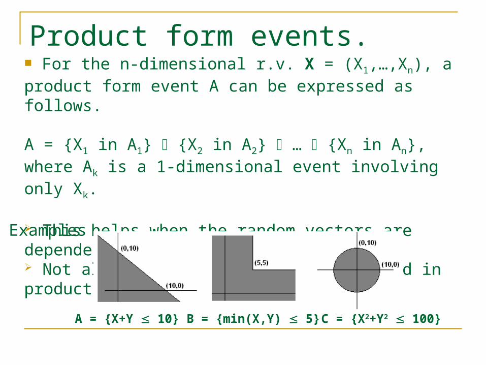
Product form events. For the n-dimensional r.v. X = (X1,…,Xn), a product form event A can be expressed as follows.

A = {X1 in A1} {X2 in A2} … {Xn in An}, where Ak is a 1-dimensional event involving only Xk.

This helps when the random vectors are dependent. Not all events can be can be expressed in product form.

A = {X+Y 10} B = {min(X,Y) 5} C = {X2+Y2 100}

Examples

Example. Let X be the input to a communication channel and let Y be the output. Input is +1 or -1 volt with equal probability. Output is the input plus a noise voltage that is uniformly distributed in the interval from -2 to +2 volts. Find the probability of positive input but not positive output.

To findP[X = +1, Y 0] = P[ {X = +1} { Y 0} ] = P[ { Y 0 } { X = +1 } ] = P[ Y 0 | X = +1] P[ X = +1]P[ X = +1 ] = ½.

When X = +1, Y is uniformly distributed in the interval [-2+1, 2+1] = [-1, 3]Now, P[ Y y | Y [-1, 3] ] = (y – (-1)) / ( 3 – (-1))Thus,P[ Y 0 | X = +1 ] = P[ Y 0 | Y [-1, 3] ] = ¼. P[ X = +1, Y 0 ] = ¼ . ½ = 1/8

Two Dimensional Random Vector Random Vector (r.v) Z = (X,Y), where

X = xj, j = 1,2,… Y = yk, k = 1,2,…Or X and Y are continuous.

Joint Distribution Function: FX,Y(x,y) = P[{X<x} ∩ {Y<y}] = P[X<x,Y<y]

Marginal Distribution Function:FX(x) = P[X<x, Y<∞] = FX,Y(x, ∞) FY(y) = P[X<∞, Y y] = FX,Y(∞, y)And FX = FY = 1 --- discrete caseOr FX = FY = 1 --- continuous case

Properties

FX,Y(-∞ ,y) = FX,Y(x,-∞) = 0

FX,Y(∞ , ∞) = 1 ----- Normalization condition.

FX,Y(x1 , y1) < FX,Y(x2 , y2) if x1<x2 and y1< y2

P[a<X<b, c<Y<d] = FX,Y(b,d) - FX,Y(b,c) - FX,Y(a,d) + FX,Y(a,c)

a, b, c and d are constants

Discrete Type Random Vectors A two dimensional discrete type r.v. has a

SZ that’s finite, or countably infinite.

SZ = SX * Y = {(xj ,yk), j = 1,2….. k = 1,2……}

Joint Probability Mass Function pX,Y(xj,yk) = P[X=xj, Y = yk] Marginal Probability Mass Functions pX(xj) = Σ pX,Y(xj,yk) and pY(yk) = Σ

pX,Y(xj,yk)

all yk all xj

Continuous Random Vector A two-dimensional r.v. Z= (X,Y) is

continuous if SZ is a uncountably infinite subset of R2.

Joint Probability Density FunctionfX,Y(x,y) = 2 FX,Y(x,y)

Marginal Probability Density Function fX(x) = ∫ fX,Y(x,y)dyProbability of event Z that belongs to A: ∫ ∫ fX,Y (x,y) dxdy

xy

A

-

Distribution Functions

For the Discrete case:

FX,Y (x,y) = Σ pX,Y(xj ,yk)

For the Continuous Case:

xjx,yky

x y

YXYX dvduvufyxF ),(),( ,,

fX,Y(x,y) = (ln x / x) if 1< x< e, 0< y<x = 0 otherwise

Example --- marginal pdf

xdyyxfdyyxfxfx

YXYXX ln),(),()(0

,,

2

1ln),()(

1

,

e

YXY dxx

xdxyxfyf

2

)(ln1),()(

2

,

ydxyxfyf

e

y

YXY

-----If 1 x e

-----If 0 < y < 1 ( x)

-----If 1 y (< x) < e

And fY(y) = 0 otherwise.

Independent Random Variables If (X,Y) is a random vector, X,Y are

independent variables if : pX,Y(xj,yk) = pX(xj) pY(yk) for discrete X,Y fX,Y(x,y) = fX(x) fY(y) for continuous X, Y FX,Y(x,y) = P[X < x ,Y< y] = FX(x) FY(y) If X and Y are independent, so are g(X),

and h(Y)

Example on marginal pmf. (discrete r.v.) A random experiment consists of tossing 2 ‘loaded’ dice and noting

the pair of numbers (X, Y) facing up. The joint pmf pX,Y(j, k) is given as

1 2 3 4 5 6

1 2/42 1/42 1/42 1/42 1/42 1/42

2 1/42 2/42 1/42 1/42 1/42 1/42

3 1/42 1/42 2/42 1/42 1/42 1/42

4 1/42 1/42 1/42 2/42 1/42 1/42

5 1/42 1/42 1/42 1/42 2/42 1/42

6 1/42 1/42 1/42 1/42 1/42 2/42

j

k

pX(j) = pX,Y(j,k) = 1/6 for all ‘j’ pX(j) = 1K=1

6

pY(k) = pX,Y(j,k) = 1/6 for all ‘k’ pY(k) = 1j=1

6

j=1

K=1

6

6

Example of dependent r.v. (discrete)In the earlier example,

pX(j) . pY(k) = 1/36 for all pairs (j, k)

But,pX,Y(j, k) = 2/42 for j = k and pX,Y(j, k) = 1/42 for j k

pX,Y(j, k) pX(j) . pY(k) for any pair (j, k) X and Y are NOT independent.

Example on marginal pdf. (continuous r.v.) Find the normalization constant ‘c’ and the marginal pdf’s

for the joint pdf given below.

fX,Y(x,y) =

Normalization condition

Ce-xe-y 0 y x <

0 elsewhere

21

0 0

cdydxecedydxece

xyxyx

C = 2

Example continued …

x

xxyxYXX eedyeedyyxfxf

0

, )1(22),()(

y

yyxYXY edxeedxyxfyf 2, 22),()(

The marginal pdf’s are given as

0 x <

0 y <

It can be verified that

0 0

1)()( dyyfdxxf YX

Example of dependent r.v. (continuous)In the previous example

fX(x) . fY(y) = 4e-xe-2y(1-e-x) 2e-xe-y = fX,Y(x, y)

Thus the r.v.’s are NOT independent

Conditional Distribution and Density Functions for Discrete

r.v. With Discrete X,Y given that Y = yk

Distribution Function:FX|Y(x|yk) = P[Xx,Y=yk]

Density FunctionpX|Y(xj|yk) = pX,Y(xj|yk) = P[X = xj ,Y = yk]

P[Y=yk]

P[Y=yk]Py(yk)

Conditional Distribution and Density

Functions for Continuous r.v With Continuous X and Y given fY(y)

Distribution Function: FX|Y(x|y) = ∫ fX,Y(u,y)du

Density Function: fX|Y(x|y) = fX,Y(x,y)

x

-∞

fY(y)

fY(y)

Example

)(2

,

2

2

)(

),()|( yx

y

yx

Y

YXX e

e

ee

yf

yxfyxf

Use of marginal pdf and joint pdf to get conditional pdf.

Let X and Y be the random variables with following joint pdf.fX,Y(x,y) = 2 e-xe-y. ( 0 y x < and 0 otherwise. )In an earlier example the marginal pdf’s were found to befX(x) = 2 e-x(1 – e-x) 0 x < andfY(y) = 2 e-2y 0 y < Find their conditional pdf’s.

x

y

xx

yx

X

YXY e

e

ee

ee

xf

yxfxyf

1)1(2

2

)(

),()|( ,

Solution :-

For x y

For 0 < y < x

Conditional Distributions & Independence

X and Y are independent if and only if the conditional distribution function, the

conditional probability mass function, or the

conditional density function of X, given the Y = y, is

identical to the marginal function.

Conditional Expectation Given that Y = y, the expectation of X is:

Discrete Case: E[X|Y=y] = Σ xjpX|Y(xj|y)

Continuous Case: E[X|Y=y] = ∫ x fX|Y(x|y)dx

The conditional expectation can be viewed as defining a function of y : g(y) = E[X | y].

Hence, g(Y) = E[X | Y] is a random variable.

j=1

∞

∞

-∞

Properties of conditional expectation. E[ E[X|Y] ] = E[X]

For the case of continuous r.v.sLet g(Y) = E[X|Y], then

XEdxxxf

dxdyyxfxdxdyyfyxfx

dyyfdxyxxfdyyfygYgE

X

YXYX

YXY

)(

),()()|(

)()|()()()(

,

This is also true for any function of X. i.e. E[ E[h(X)|Y] ] = E[ h(X) ] V[X] = E[X2] – (E[X])2 = E[E[X2|Y]]-(E[E[X|Y]])2.

Example. The total number of defects X on a chip is a Poisson variable with mean ‘’. Suppose that each defect has a probability ‘p’ of falling in a specific region ‘R’ and location of each defect is independent of the location of any other defect. Find the pmf of the number of defects Y that fall in the region ‘R’.This is a case of discrete r.v.s. If ‘k’ is the total number of defects on the chip and ‘j’ of them fall in the region ‘R’, the pmf for Y = j is given by

00

, ][]|[),(][kk

YX kXPkXjYPjkpjYP

Continued …

---- eq. (I)

Example continued …Now,P[ Y=j | X=k ] = Probability that ‘j’ defects fall in region ‘R’, given that totally there were ‘k’ defects on the chip.This is a case of binomial distribution with parameters ‘k’ and ‘p’.

P[ Y=j | X=k ] =

0, j > k

kCj pj (1 – p)K – j , 0 j k

pj

jk

kjkj

jk

k

ej

pe

kppC

kXPkXjYPjYP

!

)(

!)1(

][]|[][0

Substituting, in eq(I) and noting that ‘X’ has Poisson distribution,

Thus, the defects falling in Region ‘R’ has a Poissondistribution with Parameter‘p’.

Example. (Conditional expectation) In the last example, the number of defects falling in a specific region ‘R’ (Y) was found to have Poisson distribution with parameter ‘p’.Hence, mean of ‘Y’ = p.We can get the same result by using conditional expectation.

pXpEkXkPpkXPkp

kXPkXYEXYEEYE

kk

k

][][][)(

][]|[]]|[[][

00

0

Conditional Variance Definition,

V[X|Y] = E[(X-E[X|Y])2|Y] Another form

V[X|Y] = E[X2|Y] – (E[X|Y])2

Using the above form,E[ V[X|Y] ] = E[ E[X2|Y] ] – E[ (E[X|Y])2 ] ---- (i)And the definition of variance,V[ E[X|Y] ] = E[ (E[X|Y])2 ] – (E[ E[X|Y] ])2 ---- (ii)Adding (i) and (ii) we get a useful result. E[V[X|Y]] + V[E[X|Y]] = E[E[X2|Y]] – (E[E[X|Y]])2 =

V[X]

Functions of random variables.Let Z = X/Y. Find the pdf of Z if X and Y are independent and both exponentially distributed with mean one.We can use conditional probability.FZ(z|y) = P[Z z |y] = P[X/y z |y]

=P[X yz |y] ----- if y > 0

P[X yz |y] ----- if y < 0

=FX(yz |y) ----- if y > 0

1 - FX(yz |y) ----- if y < 0

fZ(z | y) =yfX(yz | y) ----- if y > 0

- yfX(yz | y) ----- if y < 0

= |y| fX(yz | y)

Using chain rule,dF/dz = (dF/du) . (du/dz)

Here, u = yz

Continued …

Example continued…

dyyyzfydyyfyyzfyzf YXYXZ ),(||)()|(||)( ,

Now, the pdf of Z is given by,

Using the fact that X and Y are independent and exponentially distributed with mean one,

20 1

1)(

zdyeyezf yyz

Z

Z > 0

Another example. A system with standby redundancy has a single key component in operation and a duplicate of that component in standby mode. When the first component fails the second is put into operation. Find the pdf of the lifetime of the standby system if the components have independent exponentially distributed lifetime with the same mean.Let X and Y be the lifetimes of the two components. Then the system lifetime ‘T’ is given by,T = X + YThe cdf of T is found by integrating the joint pdf of X and Y over the region of plane corresponding to the event {T t}.

xt

YXT dydxyxftF ),()( ,

Continued…

Example continued…

dxxtfxfdxxtxftFdt

dtf YXYXTT )()(),()()( ,

The pdf of T is obtained from differentiating the cdf. Further, X and Y are independent. This gives,

The two pdf’s in the integrand (exponentially distributed) are given ase-x x 0

0 x < 0fX(x) =

fY(t - x) = e-(t – x) x t

0 x > t

These substitutions give tt

xtxT tedxeetf 2

0

)()(

Expected value of functions of r.v.s E[X1 + X2 +…+Xn] = E[X1] + E[X2] +…+E[Xn]

Let X1,X2,…,Xn represent repeated measurements of the same random quantity. Then these variables can be considered iid (Independent Identically Distributed). This means, for i = 1,…,n All Xi are independent of each other.

E[Xi] = E[X] V[Xi] = V[X]

E[X1 + X2 +…+Xn] = nE[X], for iid.

V[X1 + X2 +…+ Xn] = nV[X], for iid.

Joint moment and Covariance

dxdyyxfyx YXkj ),(,

E[XjYk] = i n

niYXkn

ji yxpyx ),(,

X, Y jointly continuous

X and Y discrete

Above is the definition of jkth joint moment of X and Y If j = k = 1, it is known as correlation. If E[XY] = 0, they are said to be orthogonal. The jkth central moment of X and Y is E[(X – E[X])j (Y – E[Y])k] In the definition of jkth central moment, j = 2 and k = 0 gives V[X] while j = 0 and k = 2 gives V[Y]. In the definition of jkth central moment, j = 1 and k = 1 gives covariance of X and Y.

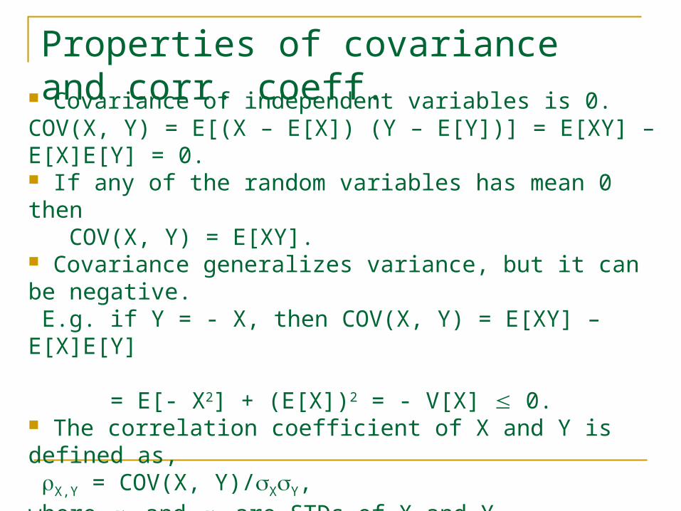
Properties of covariance and corr. coeff. Covariance of independent variables is 0.

COV(X, Y) = E[(X – E[X]) (Y – E[Y])] = E[XY] – E[X]E[Y] = 0. If any of the random variables has mean 0 then COV(X, Y) = E[XY]. Covariance generalizes variance, but it can be negative. E.g. if Y = - X, then COV(X, Y) = E[XY] – E[X]E[Y] = E[- X2] + (E[X])2 = - V[X] 0. The correlation coefficient of X and Y is defined as, X,Y = COV(X, Y)/XY, where X and Y are STDs of X and Y respectively. We have -1 X,Y 1 Correlation coefficient of independent variables is 0, but the converse is not true.

Similarly it can be proved that E[Y] = 0. Now,

Example.

0cos2

1][

2

0

dXE

Let be uniformly distributed in the interval (0,2). Define X and Y as X = cos and Y = sin.Show that the correlation coefficient between X and Y is 0.We have,

0cossin2

1]cos[sin][

2

0

dEXYE

E[XY] – E[X]E[Y] = 0 COV(X, Y) = 0 X,Y = 0

But X and Y are not independent, since X2 + Y2 = 1

Sum of random number of r.v.s Given above is the sum SN of Xi (i=1,…) iid; where N is chosen randomly and independent of each Xi. For each i, E[Xi] = E[X] and V[Xi] = V[X]. Then, E[SN] = E[N]E[X]

N

kkN XS

1

From the properties of conditional expectation,E[SN] = E[ E[SN | N] ] ------- Slide 23. = E[ NE[X] ] ------- Xi are iid’s. = E[N]E[X] ------- N is independent of each Xi.

This result is valid even if the Xi’s are not independent. They only need to have same mean.

Continued…

Continued… V[SN] = E[N]V[X] + V[N](E[X])2.

V[SN] = E[ V[SN | N] ] + V[ E[SN | N] ] ----- Slide 27.Here, V[ E[SN | N] ] = V[NE[X]] = E[N2E2[X]] – (E[NE[X]])2. = E2[X] (E[N2] – (E[N])2) = V[N] (E[X])2.And E[ V[SN | N] ] = E[NV[X]] ----- Slide 32 = E[N]V[X]Substituting in the first step above gives the expected result.

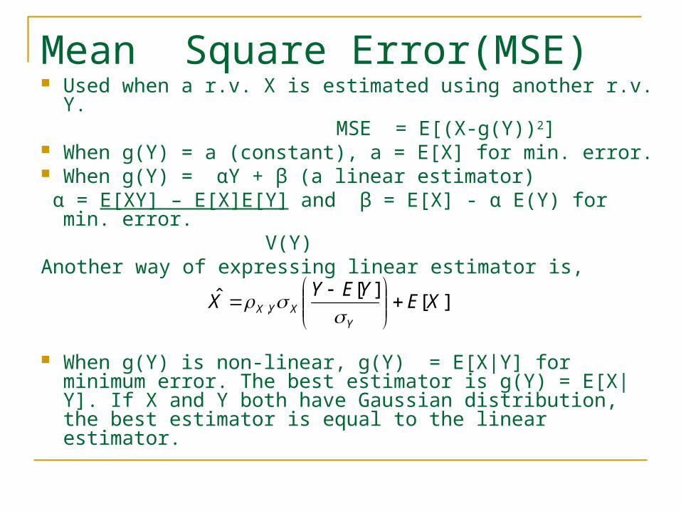
Used when a r.v. X is estimated using another r.v. Y. MSE = E[(X-g(Y))2] When g(Y) = a (constant), a = E[X] for min. error. When g(Y) = αY + β (a linear estimator) α = E[XY] – E[X]E[Y] and β = E[X] - α E(Y) for min.

error. V(Y)Another way of expressing linear estimator is,

When g(Y) is non-linear, g(Y) = E[X|Y] for minimum error. The best estimator is g(Y) = E[X|Y]. If X and Y both have Gaussian distribution, the best estimator is equal to the linear estimator.

Mean Square Error(MSE)

][][ˆ

, XEYEY

XY

XYX

Example

YX

YXYX

YX

mymymxmx

yxf,

221

2

2

2

2

2

1

1,

2

1

1

,2

,12

2)1(2

1exp

),(

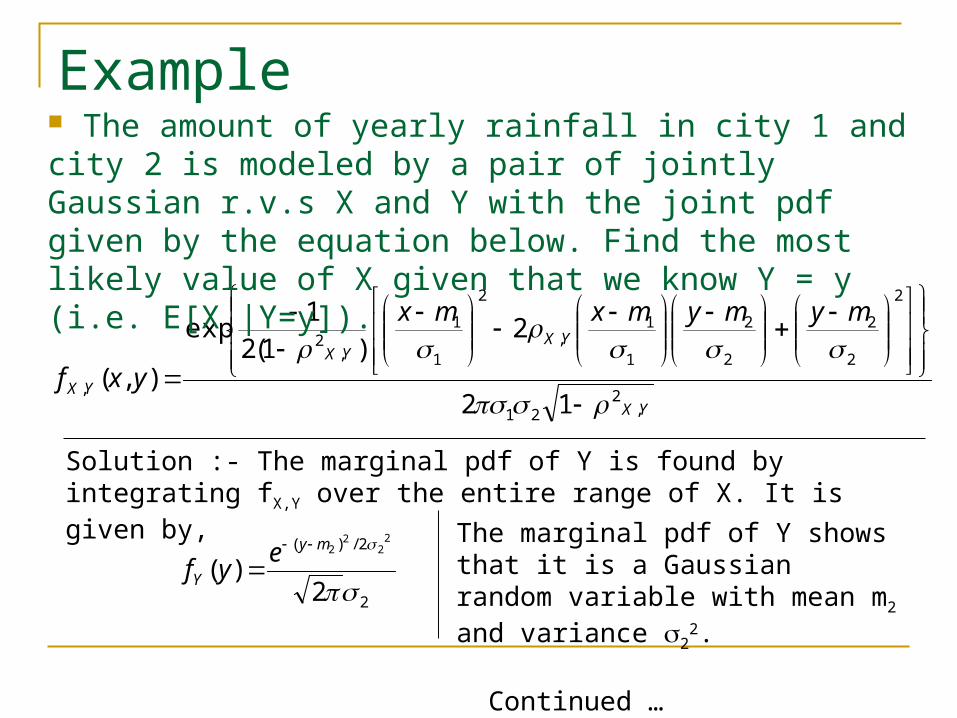
The amount of yearly rainfall in city 1 and city 2 is modeled by a pair of jointly Gaussian r.v.s X and Y with the joint pdf given by the equation below. Find the most likely value of X given that we know Y = y (i.e. E[X |Y=y]).

Solution :- The marginal pdf of Y is found by integrating fX,Y over the entire range of X. It is given by,

2

2/)(

2)(

22

22

my

Y

eyf

The marginal pdf of Y shows that it is a Gaussian random variable with mean m2 and variance 2

2. Continued …

Figures for the example.

Joint Gaussian pdf Conditional pdf of X for a fixed valueOf y.

Solution continued …Now, fX(x | y) = fX,Y(x,y) / fY(y). This can be shown to be,

)1(2

)()1(2

1exp

)|(2,

21

2

122

1,2

12,

YX

YXYX

X

mmyx

yxf

Hence, the conditional pdf of X is also Gaussian. It has a conditional mean and conditional variance given by,

E[X |Y=y] = m1 + X,Y(1/2)(y – m2) ------ (The answer to the question) AndV[X |Y=y] = (1)2(1 – (X,Y)2)

The conditional expectation found above, has an additional interpretation; which is given in the next slide.

Interpretation. Note that the conditional expectation found in the previous solution, namely, E[X |Y=y] = m1 + X,Y(1/2)(y – m2)is a function of y. Replacing ‘y’ by ‘Y’ we generate a random variable, namely, E[X | Y]. Also replacing m1 by E[X], m2 by E[Y], 1 by X, and 2 by Y, we get the following result. E[X | Y] = E[X] + X,Y(X/Y)(Y – E[Y])

We have thus proved with this example that the best estimator (LHS) is equal to the linear estimator (RHS) for jointly Gaussian r.v.s. (slide 38)

Sample mean Let X be a random variable for which the mean, E[X] = , is unknown. Let X1,…,Xn denote n independent repeated measurements of X. Then X1,…,Xn are iid’s. The sample mean defined as follows is used to estimate E[X].

n

jjn X

nM

1

1

Mn itself is a random variable and E[Mn] = , since the Xi are iid. If Sn = X1 + X2 + … + Xn, then Mn = Sn/n. V[Mn] = (1/n2)V[Sn] = V[X]/n V[Mn] 0 as n Mn becomes a good estimator as n Continued …

Sample mean continued …

2

][]|][[|

n

nn

MVMEMP

Using Chebyshev’s inequality,

Substituting for E[Mn], V[Mn] and taking the complement probability we get,

2

2

1]|[|n

MP n

This means for any choice of error and probability (1 - ), we can select the number of samples n so that Mn is within of the true mean with probability (1 - ) or greater. The quantity on the RHS of (A) gives a lower bound on probability.

----- (A)

Example A voltage of constant but unknown value is to be measured. Each measurement Xj is a sum of the desired voltage ‘v’ and a noise voltage Nj of 0 mean and STD of 1 microvolt. How many measurements are required so that the probability that Mn is within 1 microvolt of the true mean is at least 0.99?We have Xj = v + Nj

With the assumption that Xj are iid for all j, we haveE[Xj] = v and V[Xj] = 1We require = 1Substituting in (A) and replacing inequality with equality for lower bound on probability, we get0.99 = 1 – (V[Xj]/n2)Solving this we get n = 100.

Weak law of large numbers. Let X1, X2, … be a sequence of iid r.v.s with finite mean E[X] = , then for > 0,

1]|[|lim

nn

MP

The weak law of large numbers states that for a large enough fixed value of n, the sample mean using n samples will be close to the true mean with high probability.

Strong law of large numbers. Let X1, X2, … be a sequence of iid r.v.s with finite mean and finite variance, then

1lim

nnMP

The strong law of large numbers states that with probability 1, every sequence of sample mean calculations will eventually approach and stay close to E[X] = . The strong law of large numbers requires the variance to be finite but the weak law of large numbers does not.

Central Limit Theorem. Let Sn be the sum of n iid r.v.s with finite mean E[X] = and finite variance 2. Let Zn be the zero mean, unit variance r.v. defined by Zn = (Sn - n) /n, then

zx

nn

dxezZP 2/2

2

1][lim

The summands Xj need to have finite mean and variance. They can have any distribution. The resulting cdf of Zn approaches the cdf of a zero-mean, unit variance Gaussian r.v.

Example Suppose that orders at a restaurant are iid r.v.s with mean = $8 and STD = $2. After how many orders can we be 90% sure that the total spent by all customers is more than $1000?Let Xk denote the expenditure of the kth customer. Then the total spent by ‘n’ customers is, Sn = X1 + X2 + … + Xn. We have, E[Sn] = 8n and V[Sn] = 4n

The problem is to find the minimum value of ‘n’ for whichP[Sn > 1000] = 0.90

With Zn as defined in the previous slide, P[Sn > 1000] = P[Zn > (1000 – 8n)/2n] = 0.90 Continued …

Solution continued…

2/2

2

1)( z

Z ezfn

Since Zn is a Gaussian r.v. with mean 0 and variance 1, its pdf is given by

The given probability is then expressed as the following integral.

z

zn dzezZP 2/2

2

1][90.0

Where, z = (1000 – 8n)/2nThe value of ‘z’ (- 1.2815) is found from the table 3.4 in Leon –Garcia and the minimum value of ‘n’ is found by solving the quadratic equation in n, namely, 8n – 1.2815(2)n – 1000 = 0.The positive root of this quadratic equation gives n = 128.6

Thus after minimum 129 orders we can be 90% sure that the total spent by customers is more than $1000.

Questions???