arX

iv:1

404.

4798

v2 [

q-fi

n.PM

] 6

Aug

201

4

Signal-wise performance attribution for

constrained portfolio optimisation

Bruno Durin1

1 Capital Fund Management, 23-25 rue de l’Université, Paris, France

Abstract

Performance analysis, from the external point of view of a client who wouldonly have access to returns and holdings of a fund, evolved towards exact at-tribution made in the context of portfolio optimisation, which is the internalpoint of view of a manager controlling all the parameters of this optimisation.Attribution is exact, that-is-to-say no residual “interaction” term remains, andvarious contributions to the optimal portfolio can be identified: predictive sig-nals, constraints, benchmark. However constraints are identified as a separateportfolio and attribution for each signal that are used to predict future re-turns thus corresponds to unconstrained signal portfolios. We propose a novelattribution method that put predictive signals at the core of attribution andallows to include the effect of constraints in portfolios attributed to every sig-nal. We show how this can be applied to various trading models and portfoliooptimisation frameworks and explain what kind of insights such an attributionprovides.

1 Introduction

Performance analysis is at the core of investment process. The pioneering ap-proaches, be they return-based or portfolio-based, took a external stance, aiming atexplaining performance with the same data that an investor would have from a fundmanager: returns and holdings. These are the long-standing models of performanceanalysis (Sharpe, 1966; Jensen, 1968; see also references in Grinold & Kahn, 1999)and of factor models (Fama-French, 1993, and subsequent works) using only time se-ries of returns on the one hand, and the more recent approaches of performance attri-bution pioneered by Brinson, Hood & Beebower (1986); Brinson, Singer & Beebower(1991) using both returns and holdings on the other hand.

Return based analysis can be summarised as a regression of fund returns overwell chosen and meaningful time series of returns. The coefficients of the regressionprovide an quantitative assessment of what the manager is doing. As a very simpleexample, we can check that an index tracker does not have a large cap bias bychecking its exposure to the size factor or that a global fund whose prospectus claimsbalanced exposures to developed markets does not show any oversized exposure to,say, US markets.

1

Holding based analysis in principle allows for a finer understanding of what themanager is doing. The Brinson et al. model decomposes the active return1 alongcategories, which originally were sectors, into three components: the allocation part,which corresponds to a strategy that trades benchmark sectors as a whole, theselection part, which corresponds to stock weighting inside a given sector and aninteraction part, which simply is the unexplained part. This methodology can beextended to several layers of decision making according to various categories as canbe exemplified by industry implementation such as Morningstar’s one (Morningstar,2011, 2013). However as it is difficult to extend to several categories, a more generalframework for performance attribution may be preferred: we regress over portfoliocharacteristics that can be anything relevant for the analysis, predictive signals asin (Grinold, 2006) or various factor scores2 for example. In (Grinold, 2006) thesecharacteristics are translated into portfolios, which allows to express the results interm of risks, correlations and (co-)variances. As it has been noted that Brinsonmodel can be seen as a regression (Lu & Kane, 2013), we shall consider the variousholding-based analyses as regressions.

At this point, whatever the level of details at which we perform our analysis, weare basically doing regressions, which have a major drawback: the residual unex-plained part may be large. Furthermore, adding many factors to reduce it may leadto in-sample bias and may reduce the explanatory power of the analysis. As shownin the example given in (Grinold, 2006), a portfolio built from three signals, a fastone, an intermediate one and a slow one, while taking into account transaction costs,can be explained with a R2 of 87%. Of course in this case the residual variance issmall enough for the analysis to be valuable: it is clear that the portfolio overweightsintermediate and slow signals with respect to the ideal, no-cost portfolio, in orderto reduce costs as expected. But in the general case the unexplained part can be solarge that it is barely possible to conclude anything. Namely this is the case whenconstraints are imposed on the portfolio and we cannot enlarge them to come to amore amenable situation.

By taking an internal point of view, which means by assuming that not onlywe have access to returns and holdings of the fund but also to the optimisationprocedure used to build the portfolio, we can tackle this problem. In their seminalpaper (Grinold & Easton, 1998) the authors exactly decompose the performanceof a portfolio obtained by constrained mean-variance optimisation into a bench-mark part, a signal part and a constraint part. As we shall rephrase it later, thecore of the method consists in splitting the optimality equation (KKT3 condition)into the corresponding terms that can be expressed as what is called in the articlecharacteristics portfolios. Subsequent works (Grinold, 2005; Scherer & Xu, 2007;Stubbs & Vandenbussche, 2008; Bender, Lee & Stefek, 2009) suggested variationsand improvements of the method, studying the effect of constraints on key quan-tities such as information ratio or utility function, addressing alpha misalignmentcaused by constraints or taking into account non-linear and/or non-differentiable

1return over a benchmark2for example we could carry a sector, size, value and momentum analysis3Karush-Kuhn-Tucker, see for example Boyd & Vandenberghe (2004) p. 243 and references

provided p. 272

2

convex constraints or objective function terms.Even if these techniques allow exact performance attribution, constraints can

only be tackled as separate entities. Let us illustrate this point through a concreteexample: a fund manager would like to offer a style shifting value and momentumlong-only product to, say, institutional investors. What we mean by style shifting isthe fact that the manager has the discretionary power to adjust the relative weight ofvalue and momentum strategies by monitoring their recent performance for example.We assume that the manager knows how to compute value and momentum predictivesignals and for a given signal or combination of signals how to build a long/shortportfolio through a risk constrained optimisation and a long-only portfolio througha risk and no-short constrained optimisation4. How could he build his new product?

One obvious and simple solution would be to add the value long-only portfolioand the momentum long-only portfolio. By monitoring the performance of eachportfolios, we would adjust the relative risk attributed to each. But that would begreatly sub-optimal, especially given the fact that value and momentum are anti-correlated5, which means that when a position in the value long/short portfoliois long, one expects that the corresponding position in the momentum long/shortportfolio is short, but by imposing long-only constraints to both portfolios, we cannotbenefit from crossing: if we imposed the constraint on the total portfolio, momentumcould take a short position as large as long value position is. If he builds the portfoliothis way, by adding predictive signals and running a constrained optimisation tocompute the total portfolio, he will run into a different problem: how to attributeperformance to value and momentum? The aforementioned techniques allows toattribute a performance to the long-only constraints, but this is likely to be almost aslarge as the unconstrained value and momentum performances. If the total portfoliois losing money, given the fact that we cannot relax the long-only constraints andassuming that unconstrained value and momentum have both positive performance,which one to cut? In other words, which strategy is most affected by the constraints?

Falling back on regression method is not a solution as it is likely to be use-less due to a large residual, be the regressors long/short portfolio performances orlong-only ones. Using the exact performance attribution where the constraints aretranslated into a characteristics portfolio, it’s hard to understand the link betweenthe raw performance of a signal and its performance in the constrained portfoliooptimisation.

What is usually done in such a case is to use a somewhat ad-hoc scheme toattribute the performance to the signals and to avoid introducing a constraint port-folio whose performance is as large as the one of the signals. It’s far easier to makean investment decision based on this attribution. It is not hard to find reasonableschemes of attribution. For example we could attribute a constraint p&l propor-tionally to signal absolute size or give a rule to split the total trade into a “value”trade and a “momentum” trade. But how to advocate them? Which one to chooseif two perfectly reasonable schemes lead to contradictory results (in our case study

4For long-only portfolios the risk constraint would rather be replaced by a tracking error riskconstraint and the optimisation be done on portfolio positions relative to benchmark ones, butthese are implementation details that are not relevant for the given example.

5see for example Asness, Moskowitz & Pedersen (2013)

3

positive and negative performance for the value part of the portfolio for example)?In this article, we propose an exact signal-wise performance attribution in pres-

ence of constraints that allows to overcome the shortcomings of the previous method.Instead of translating the effect of constraints into implied alphas (which is anotherview of the characteristics portfolios), we show how to translate it into implied costsand risk. To our knowledge, this is the first attempt in this direction. Even thoughthe technique we describe is by no mean the final answer of the problem, it natu-rally stems from the properties of the problem that we consider and, as an addedbonus, yields simple interpretation of the effect that some constraints and terms inthe objective function have on the signals.

2 Yet another look at the Lagrange multipliers

2.1 General trading framework

In this section, we shall review the method of attribution published in (Grinold & Easton,1998). We shall use the dynamic trading framework of Gârleanu & Pedersen (2013)as a general setting in which to apply the technique. All notations are the sameas in their article. Building upon our case study of a long-only style shifting valueand momentum fund, we shall consider the following model, which is also given asan example in a more general form (example 2, section V in Gârleanu & Pedersen(2013)):

rt+1 = Bft + ut+1 , (1)

where r is the vector of the price changes in excess of the risk-free return of the Nequities in our investment universe, u is the unpredictable noise and f is a 2N × 1

vector of predictive signals(

vt mt

)Twith vt (resp. mt) the vector of value (resp.

momentum) signals for all stocks. B is a N × 2N matrix, which for simplicity wewill be assume to be N ×N block diagonal, such that we can write for each stock i

rit+1 = bivvit + bimm

it + ui

t+1 . (2)

Redefining vit as bivvit and similarly mi

t, we can simply write the returns as the sumof our two signals and a noise

rit+1 = vit +mit + ui

t+1 . (3)

In the general case we will define K vectors gk for k = 1, . . . , K by (gk)it = Bikf

kt in

order to write the returns as the sum of K predictive components and a noise

rt =∑

k

gkt + ut+1 = Gt + ut+1 . (4)

The present value of all future expected excess returns penalised for risk and tradingcosts is maximised by solving a Bellman equation, which is not reproduced here.Taking into account the known solution for the value function and integrating theeffect of the dynamics of the predictive signals in their definition, it is not difficult tosee that it can be expressed as a quadratic optimisation problem in the trade ∆xt:

max∆xt

−1

2∆xtQ∆xt −∆xtPxt−1 +∆xtGt , (5)

4

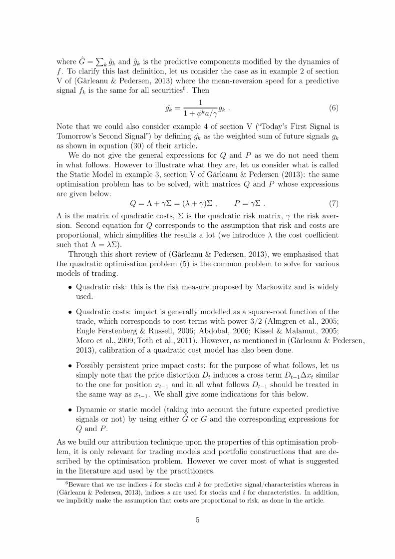
where G =∑

k gk and gk is the predictive components modified by the dynamics off . To clarify this last definition, let us consider the case as in example 2 of sectionV of (Gârleanu & Pedersen, 2013) where the mean-reversion speed for a predictivesignal fk is the same for all securities6. Then

gk =1

1 + φka/γgk . (6)

Note that we could also consider example 4 of section V (“Today’s First Signal isTomorrow’s Second Signal”) by defining gk as the weighted sum of future signals gkas shown in equation (30) of their article.

We do not give the general expressions for Q and P as we do not need themin what follows. However to illustrate what they are, let us consider what is calledthe Static Model in example 3, section V of Gârleanu & Pedersen (2013): the sameoptimisation problem has to be solved, with matrices Q and P whose expressionsare given below:

Q = Λ+ γΣ = (λ+ γ)Σ , P = γΣ . (7)

Λ is the matrix of quadratic costs, Σ is the quadratic risk matrix, γ the risk aver-sion. Second equation for Q corresponds to the assumption that risk and costs areproportional, which simplifies the results a lot (we introduce λ the cost coefficientsuch that Λ = λΣ).

Through this short review of (Gârleanu & Pedersen, 2013), we emphasised thatthe quadratic optimisation problem (5) is the common problem to solve for variousmodels of trading.

• Quadratic risk: this is the risk measure proposed by Markowitz and is widelyused.

• Quadratic costs: impact is generally modelled as a square-root function of thetrade, which corresponds to cost terms with power 3/2 (Almgren et al., 2005;Engle Ferstenberg & Russell, 2006; Abdobal, 2006; Kissel & Malamut, 2005;Moro et al., 2009; Toth et al., 2011). However, as mentioned in (Gârleanu & Pedersen,2013), calibration of a quadratic cost model has also been done.

• Possibly persistent price impact costs: for the purpose of what follows, let ussimply note that the price distortion Dt induces a cross term Dt−1∆xt similarto the one for position xt−1 and in all what follows Dt−1 should be treated inthe same way as xt−1. We shall give some indications for this below.

• Dynamic or static model (taking into account the future expected predictivesignals or not) by using either G or G and the corresponding expressions forQ and P .

As we build our attribution technique upon the properties of this optimisation prob-lem, it is only relevant for trading models and portfolio constructions that are de-scribed by the optimisation problem. However we cover most of what is suggestedin the literature and used by the practitioners.

6Beware that we use indices i for stocks and k for predictive signal/characteristics whereas in(Gârleanu & Pedersen, 2013), indices s are used for stocks and i for characteristics. In addition,we implicitly make the assumption that costs are proportional to risk, as done in the article.

5

In all what follows we do not distinguish between various models. Namely G willnot be distinguished from G.

2.2 Linearity

The key property of the optimality equation of (5)

Q∆xt + Pxt−1 = Gt (8)

is linearity. Q∆ + P is a linear operator over the time series {xt} of all positions7.Linearity allows us to write the solution xt as

xt =∑

k

xkt (9)

where xkt is the solution of the same equation with the source term Gt replaced by

component gktQ∆xk

t + Pxkt−1 = gkt . (10)

Computing the solution is straightforward through a iterative process. Let us startat t = 0 with zero total position x0 = 0 and zero position on all components xk

0 = 0.We compute each trade component:

∆xkt = Q−1(gkt − Pxk

t−1) (11)

and update each position components

xkt = xk

t−1 +∆xkt . (12)

Should we add a persistent impact, we would assume that at t = 0, total price dis-tortion is D0 = 0 and its components Dk

0 = 0 and we would update each componentswith the evolution equation for the price distortion8: Dk

t+1 = (I −R)(Dkt + C∆xk

t ).The meaning of the notations is given in (Gârleanu & Pedersen, 2013) and is notcrucial for what we explain. We update trades and positions for every signal, whosesum is exactly the total optimal trade and total optimal position (9).

We remind that such an attribution has already been described in (Grinold & Easton,1998). We insist on the fact that it merely is a consequence of the linearity of ouroptimality equation and could be applied to any optimisation problem, convex ornot, whose optimality equation is linear.

Through linearity, we get a direct unambiguous and exact attribution to thevarious components, which are added up to predict the future returns. From theposition time series {xk

t } it is straightforward to compute a p&l and to attributerisk and costs following (Litterman, 1996) or (Bruder & Roncalli, 2012):

R = xtΣxt =∑

k

(xktΣxt) =

∑

k

Rk (13)

7In a continuous time setting, we would have a linear first order differential equation withunknown function x(t).

8Evolution equation of D encodes a linear exponential kernel operator on trades {∆xu}u6t

which would replace operator Q∆. When linearity property is applied to the resulting optimalityequation, it translates into splitting D into K components Dk.

6

and

C =1

2∆xtΛ∆xt =

∑

k

(

1

2∆xk

tΛ∆xt

)

=∑

k

Ck . (14)

2.3 Constraints and additional terms in the objective func-

tion

The linearity property of optimality equation indeed allows us to attribute tradesand positions to various constraints as the authors of (Grinold & Easton, 1998) didin introducing their characteristic portfolios. Not all constraints fit in this frame-work, but most of those used in portfolio optimisation do. If we let aside combina-torial constraints (number of trades, round-lots, etc.) and non convex constraints(minimum trade size for example), the usual suspects are:

• minimum and maximum trade, minimum and maximum position

mi 6 ∆xt 6 Mi mi 6 xt−1 +∆xt 6 Mi (15)

where usually mi = −Mi (that is to say, only trade or position size is con-strained),

• minimum and maximum exposure of the portfolio

m 6 (xt−1 +∆xt) · v 6 M (16)

where v is a vector encoding the exposure. As an example, for a sector expo-sure, v would be 1 for stocks belonging to the given sector and 0 elsewhere. An-other example can be found in the usual formulation of the minimum-varianceproblem where the constraint that net exposure should be 1 is imposed: vwould be a vector of 1 and we should set m = M = 1 (and prediction G = 0).Last example, imposing market neutrality would lead us to choose v as the vec-tor of stock betas. Exposure constraints are pervasive in portfolio optimisationproblems.

All these constraints can be written as f(∆xt) 6 M where f is a linear function of∆xt: let v be the vector such that f(∆xt) = v ·∆xt. We shall label constraints withindex c and consider the collections of constraint vectors vc and bounds Mc.

We now turn back to our optimisation problem (5), which we add constraintsto. This is straightforward for the static model. For the dynamic model consideredin (Gârleanu & Pedersen, 2013), constraining only the next-step optimisation of∆xt while using the unconstrained solution of the Bellman equation for the valuefunction is a standard approximation (see as examples Sznaier & Damborg, 1987;Skaf & Boyd, 2008). Constrained dynamic programming problems are notoriouslydifficult to solve9 and will not be considered here. Introducing Lagrangian multipliersλc as done in (Grinold & Easton, 1998), optimality equation (8) becomes

Q∆xt + Pxt−1 = Gt +∑

c

λct . (17)

9but see (Bemporad et al., 2002) in which the authors show that control policy for linear con-straints are linear functions f(y) = Ay + b of the state (Gt, xt−1), which let us think that what isdescribed in this article is also applicable when the value function is not approximated.

7

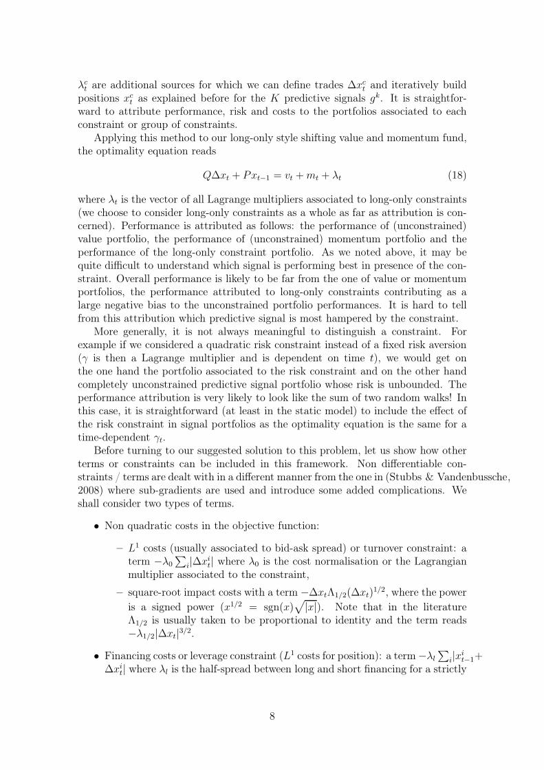
λct are additional sources for which we can define trades ∆xc

t and iteratively buildpositions xc

t as explained before for the K predictive signals gk. It is straightfor-ward to attribute performance, risk and costs to the portfolios associated to eachconstraint or group of constraints.

Applying this method to our long-only style shifting value and momentum fund,the optimality equation reads

Q∆xt + Pxt−1 = vt +mt + λt (18)

where λt is the vector of all Lagrange multipliers associated to long-only constraints(we choose to consider long-only constraints as a whole as far as attribution is con-cerned). Performance is attributed as follows: the performance of (unconstrained)value portfolio, the performance of (unconstrained) momentum portfolio and theperformance of the long-only constraint portfolio. As we noted above, it may bequite difficult to understand which signal is performing best in presence of the con-straint. Overall performance is likely to be far from the one of value or momentumportfolios, the performance attributed to long-only constraints contributing as alarge negative bias to the unconstrained portfolio performances. It is hard to tellfrom this attribution which predictive signal is most hampered by the constraint.

More generally, it is not always meaningful to distinguish a constraint. Forexample if we considered a quadratic risk constraint instead of a fixed risk aversion(γ is then a Lagrange multiplier and is dependent on time t), we would get onthe one hand the portfolio associated to the risk constraint and on the other handcompletely unconstrained predictive signal portfolio whose risk is unbounded. Theperformance attribution is very likely to look like the sum of two random walks! Inthis case, it is straightforward (at least in the static model) to include the effect ofthe risk constraint in signal portfolios as the optimality equation is the same for atime-dependent γt.

Before turning to our suggested solution to this problem, let us show how otherterms or constraints can be included in this framework. Non differentiable con-straints / terms are dealt with in a different manner from the one in (Stubbs & Vandenbussche,2008) where sub-gradients are used and introduce some added complications. Weshall consider two types of terms.

• Non quadratic costs in the objective function:

– L1 costs (usually associated to bid-ask spread) or turnover constraint: aterm −λ0

∑

i|∆xit| where λ0 is the cost normalisation or the Lagrangian

multiplier associated to the constraint,

– square-root impact costs with a term −∆xtΛ1/2(∆xt)1/2, where the power

is a signed power (x1/2 = sgn(x)√

|x|). Note that in the literatureΛ1/2 is usually taken to be proportional to identity and the term reads−λ1/2|∆xt|

3/2.

• Financing costs or leverage constraint (L1 costs for position): a term −λl

∑

i|xit−1+

∆xit| where λl is the half-spread between long and short financing for a strictly

8

market neutral portfolio10 or the Lagrangian multiplier associated to the con-straint.

Note that L1-terms may appear even in absence of any financial costs in the prob-lem: they can be introduced as regularisation terms in the context of a lassoregression (Tibshirani, 1996). For an application to portfolio optimisation, see(DeMiguel et al., 2009), which focuses on minimum variance portfolio, and the morerecent (Bruder et al., 2013).

Square-root impact costs are considered in the appendix. We shall here focus onthe L1 terms / constraints. When such terms are added, the optimisation problem(5) can be turned into a more simple one by introducing auxiliary variables. This isa standard procedure (see Boyd & Vandenberghe (2004) section 6.1.1 example “Sumof absolute residuals approximation” or (Lobo Fazel & Boyd, 2007) for a variant thatis more suitable for constraints only on short or long positions). The optimisationproblem:

max∆xt

−λ0

∑

i

|∆xit| − λl

∑

i

|xit−1 +∆xi

t| −1

2∆xtQ∆xt −∆xtPxt−1 +∆xtGt (19)

is equivalent to the following one

max∆xt,s,u

−λ0

∑

i

si − λl

∑

i

ui −1

2∆xtQ∆xt −∆xtPxt−1 +∆xtGt

−si 6 ∆xit 6 si

−ui 6 xit +∆xi

t 6 ui .

(20)

The additional constraints are also linear in ∆xit which means that the Lagrangian

multipliers ξc associated to them will appear as additional sources of the linearoptimality equation:

Q∆xt + Pxt−1 = Gt +∑

c

ξct (21)

where c indexes the type of constraint such that ξct is the vector of all Lagrangianmultipliers associated the constraints of the given type applied to each stock.

Cost attribution can be generalised in the following way:

− λ0|∆xt| = −∑

k

[

λ0∆xkt sgn(∆xt)

]

(22)

and− λl|xt−1 +∆xt| = −

∑

k

[

λl(xkt−1 +∆xk

t ) sgn(xt−1 +∆xt)]

(23)

where we define sgn(y) = 0 for y = 0.

10In a more general setting, financing of the long positions and financing of the short positionslead to two distinct terms, the first being function of (xi

t−1 + ∆xit)+ = max(xi

t−1 + ∆xit, 0) =

1

2

(

xit−1 +∆xi

t+ |xi

t−1 +∆xit|)

and the second being function of (xit−1 + ∆xi

t)−

= min(xit−1 +

∆xit, 0) =

1

2

(

xit−1 +∆xi

t − |xit−1 +∆xi

t|)

. An optimisation problem with such terms can also beturned into a more simple one as described after.

9

With standard performance attribution that associates a portfolio to each con-straint type, it is hard to get a clear interpretation of these terms. As there is aportfolio associated to spread costs for example, the decomposition of costs in thep&l attributes quadratic costs and spread costs to this portfolio as it does to theothers (portfolios associated to signal components and to other constraints). Whatis the meaning of quadratic costs for the portfolio associated to spread costs? Whatare these spread costs associated to spread cost portfolio? Has this question evengot a meaning?

What is the interpretation of the risk associated to spread cost portfolio? Forthis question we could make an educated guess: we could understand it as a riskreduction associated with the costs that prevents us from making trades as big aswe would have done if these additional costs were not present.

Nevertheless, the asymmetry that such a decomposition introduces betweenquadratic costs and spread costs is hard to justify. It would be more natural todirectly get the combined effect of quadratic and spread costs on a given signal.

3 Signal-wise attribution of constraints

3.1 Effective quadratic costs and effective quadratic risk

It is now clear that we would like an exact attribution that does not introduceadditional portfolios for constraints or terms that are converted into constraints. Weshall show that we are able to express all the constraints and additional terms thatwe listed in the previous section as effective quadratic costs and effective quadraticrisk. The optimality equation will have the form

Qt∆xt + Ptxt−1 =∑

k

gkt (24)

where the only source terms are the predictive signals. To our knowledge, thetechnique we shall describe is original, but the idea of considering the effect ofconstraints as a deformation of the quadratic risk has already been presented. In(Jagannathan & Ma, 2003; Roncalli, 2011), the authors show how minimum andmaximum position constraints can be seen as a shrinkage of the covariance matrixused in the optimisation problem. The key element that allows them to do this is aconstraint on the net exposure of the portfolio: 1 · xt = 1. Building upon this idea,the author of (de Boer, 2012) generalises the work of (Jagannathan & Ma, 2003) byshowing how constraints imply a “shrinkage estimate” of the mean and covarianceof returns. His work allows to consider more general constraints but as it uses thesame mathematical framework it suffers from the same shortcomings.

We present a generalisation of these results through a new method. First ofall we take into account transaction costs and show how some very widespreadconstraints translate into effective quadratic costs. Furthermore in our frameworkthere is no need for any specific constraint (such as 1 · xt = 1) that in the previousworks is key to build the effective risk matrix. Last but not least we do not affectthe estimation of the mean of returns: there is no such notion as implied alpha orshrunk alpha, as to our mind managers do not use constraints to improve return

10

estimations, but rather to control for the effect of a bad risk estimation (namelyinverting a badly estimated risk matrix as done in Markowitz optimisation problemintroduces a lot of noise). By taking full advantage of the mathematical propertiesof the optimisation problem, we developed an original method that is less dependenton some specific characteristics of the problem and that allows for a more direct andnatural attribution11.

All constraints and terms we considered in last section can be put under a linearconstraint form,

v ·∆xt 6 M (25)

at the expense of introducing auxiliary variables in some cases. We shall explicitlydistinguish between constraints on trade and constraints on position

v · (xt−1 +∆xt) 6 M (26)

We shall describe the technique on position constraints. Adaptation to trade con-straints is straightforward.

Generally speaking, constraints will go in pairs:

m 6 v · (xt−1 +∆xt) 6 M (27)

One of the following constraint

(v · (xt−1 +∆xt))26 m2 or (v · (xt−1 +∆xt))

26 M2 (28)

is equivalent the previous one: when upper bound and lower bound are defined,only one of the bounds is active at the same time. Now let us introduce Lagrangianmultipliers η for the equivalent constraint. The KKT conditions for optimalityconsist in finding the critical point of augmented objective function F

F = −1

2∆xtQ∆xt −∆xtPxt−1 +∆xtGt − η (xt−1 +∆xt) v ⊗ v (xt−1 +∆xt) (29)

In the static model where Q is the sum of quadratic costs Λ and penalisedquadratic risk γΣ and P is the penalised quadratic risk, it is obvious that under sucha form the position constraint is equivalent to an additional quadratic risk 2η/γ v⊗v.Effective quadratic risk is thus Σ + 2η/γ v ⊗ v. Interpretation is the following: if aconstraint is violated, we add a factor to the risk model, whose strength we tune toreduce the exposure to the authorised level. If the constraint is a simple minimumor maximum position m 6 xt 6 M , the effective risk that it introduces simply is anad-hoc idiosyncratic risk for the stock. If we have only constraints on positions, it iseasy to see that we effectively perform a shrinkage towards a diagonal risk matrix.We get a result that yields the same interpretation as in (Jagannathan & Ma, 2003).Furthermore, as we showed that adding constraints is equivalent to adding factors inthe risk model, we can shed new light on the factor alignment problems: reversing theprocess, we could try to understand the solutions advocated in (Lee & Stefek, 2008;

11As it will be obvious in what follows, it is also straightforward to see that the effective riskmatrix is positive-definite and to come to the shrinkage interpretation of the original quadraticrisk matrix towards a diagonal risk matrix.

11

Bender, Lee & Stefek, 2009; Saxena & Stubbs, 2010, 2013; Ceria Saxena & Stubbs,2012) in terms of constraints on the non-aligned part of the optimal portfolio.

Squaring trade constraints will lead to effective quadratic costs, whose interpre-tation is even more straightforward.

In the dynamic trading framework, position (resp. trade) constraints also leadto effective quadratic risk (resp. costs) but the expression of the effective quadraticrisk (resp. costs) as a function of the original quadratic risk (resp. costs) and thepenalty term introduced by the constraint is not simple to establish in the generalcase. This could be the purpose of a future work.

In the presence of all constraints, the optimality equation reads

(Q+∑

c

µctAc +

∑

c′

ηc′

t Ac′)∆xt + (P +∑

c′

ηc′

t Ac′)xt−1 =∑

k

gkt (30)

which is the form (24) that we announced before, provided one defines Qt and Pt as

Qt = Q +∑

c

µctAc +

∑

c′

ηc′

t Ac′

Pt = P +∑

c′

ηc′

t Ac′

(31)

As for notations, c indexes trade constraints, c′ indexes position constraints. µc

are the Lagrangian multipliers associated to squared trade constraints, whereas ηc′are those associated to squared position constraints. Matrices Ac are defined as2 vc ⊗ vc. For example in the simple case of a minimum or maximum trade orposition constraint on stock i, Ac is a matrix whose diagonal element i, i is equal to1 and whose all other elements are 0.

3.2 Attribution

We established a linear equation (24) whose only source terms are the predictivesignals. As explained in subsection 2.2, we can directly attribute trades and positionsto the K signals. We obtain K portfolios, one for each signal, which includes theeffect of constraints and cost terms. Risk and costs attribution is now only doneover the predictive signal portfolios, which avoids some of the inconsistencies wementioned earlier.

Let us explicitly work out our running example of the long-only style-shiftingvalue and momentum fund. Risk is effectively increased on all positions that wouldbe short12 in absence of the long-only constraints until they are equal to 0. Letus call C the set of stocks for which long-only constraint is active and define ρt adiagonal matrix whose diagonal element i, i is equal to 2ηit if i ∈ C else 0. Optimalityequation (24) reads

(Q+ ρt)∆xt + (P + ρt)xt−1 = vt +mt (32)

12Let us remind that positions are over the benchmark so long-only constraints are in fact lowerbounds that are equal to minus the benchmark positions.

12

Let us assume for simplicity that costs are proportional to risk, that risk is diagonalΣ = σ2 and that we are using the static model. In this case, in the absence ofconstraints:

∆xt =γσ2

γσ2 + λ(x0

t − xt−1) (33)

where x0t is the Markowitz solution Gt/(γσ

2). In the presence of constraints, ourattribution technique yields two trades for value and momentum

∆xv,t =γσ2 + ρt

γσ2 + ρt + λ(x0

v,t − xv,t−1)

∆xm,t =γσ2 + ρt

γσ2 + ρt + λ(x0

m,t − xm,t−1)

(34)

In the expression for x0v,t and x0

m,t, γσ2 is replaced by γσ2 + ρt. If a stock is con-

strained, its aim position13 x0 is reduced in absolute value and the trade will tendto get closer to this corrected aim so that constraint is fulfilled. The impact of theconstraint on value and momentum trade depends not only on signal strength orthe aim position but also on the current position reached by previous trades.

Returning to the general interpretation as effective risk, for constrained stocksvalue and momentum signals are run with an effectively higher risk aversion, whichmeans that even if the trade of one of the two signals is in the right direction (long fora minimum position constraint), it is affected by the constraints. This is in contrastto a more naive ad-hoc attribution that for example would consist in computingunconstrained signal trades and in cutting only the one going short. But that isexactly the difference between seeing constraints as a shift in predicted returns14

and seeing (position) constraints as a shrinkage of risk estimation.This direct and exact signal-wise attribution allows us to track performance, risk

and costs for each predictive signals. We are able to make decisions such as signalweighting even in presence of strong constraints. We are also able to compute atransfer coefficient for each predictive signal and either drop signals whose coeffi-cient is too low, meaning that constraints are too strong for them to deliver theirperformance in presence of other signals, or relieve some constraints to let signals“breathe” better. As an example a manager could adjust constraints so that a factoror style timing strategy really has a value-added or our manager running a valueand momentum long-only fund could realise that constraints make the addition of,say, a growth strategy useless.

3.3 How to compute effective costs and risk?

Let us come back to a more practical point of view. How are the Lagrangian multi-pliers of squared constraints, which we shall call attribution multipliers in contrastwith the Lagrangian multipliers of original constraints, computed?

Firstly let us note that we could in principle design an ad-hoc penalty-like opti-misation algorithm that would work as follows:

13as named in (Gârleanu & Pedersen, 2013)14Shifted alpha is called implied alpha in the literature.

13

• compute unconstrained optimal trades

• for all trades (resp. positions) that violate a constraint, add a penalty termηc∆xtAc∆xt (resp. ηc(xt−1 +∆xt)Ac(xt−1 +∆xt))

• compute the corresponding optimal trades

• update ηc until constraints are fulfilled

Such a naive algorithm provides no convergence bound. As the original constrainedproblem is convex in most of the cases, it would be a pity that we could not usethe power of the numerous algorithms that exist to solve it. One of the specificcases where the ad-hoc algorithm might be interesting is the minimum trade sizeconstraint, which is not convex. This might be handled by allowing ηc to be negative,that is to say to allow for negative effective costs. Indeed if a non zero trade isrounded up to the minimum trade size, this amounts to compute an unconstrainedtrade with smaller quadratic costs: hence negative costs have been added to theoriginal quadratic costs. We shall not pursue this idea here and shall only considerconvex constraints.

From this point, we shall assume that the constrained optimisation problem hasbeen solved by an algorithm that provides both optimal trades and Lagrange mul-tipliers λc of the original constraints. Lagrange multipliers encode the marginalvariation of the objective function at the optimum for a marginal variation of con-straint bound:

λc = ǫ∂F⋆

∂Mc(35)

where ǫ is a sign, equal to +1 if the constraint is an upper bound15 and equal to −1if the constraint is a lower bound. For attribution multipliers, we have

ηc =∂F⋆

∂(M2c )

(36)

where sign is always +1 as M2c is always an upper bound and we have the same F⋆ as

it is an equivalent optimisation problem leading to the same solution. As ∂/∂(M2c ) =

1/(2Mc)∂/∂Mc, we get the following relationship between both multipliers

ηc = ǫ1

2Mcλc . (37)

It can be checked that under mild assumptions if constraints are correctly split intotrade and position constraints, ηc is positive. Or we can pragmatically turn thisaround for non straightforward cases, choose to see the constraint as a trade (aneffective cost) or a position (an effective risk) constraint so that the correspondingmultiplier is positive. For this to be always possible, the constraint must reduceeither the trade or the position, which is the case for all trade and position constraintswhose admissible space contains 0. The relationship (37) can also be understood in a

15The given signs correspond to a maximisation problem.

14

way reminiscent of what is done in (Jagannathan & Ma, 2003)16: we introduce in theoriginal optimality conditions an explicit dependence on trade for a trade constraint(and similarly for a position constraint) by using the following substitution

1 =2v ·∆xt

2Mc

, (38)

which is true whenever the constraint is saturated. For example the λcvc term thatwould appear in the original optimality equation for an upper bound constraint ontrade can be turned into 2 ηc v ⊗ v∆xt. If the constraint is saturated the previousequation holds, otherwise λc and ηc are zero.

From the solution provided by the algorithm, which we assumed to provideLagrangian multipliers, it is straightforward to compute attribution multipliers, tobuild the optimality equation (24) and to perform the signal-wise attribution.

The relationship (37) highlights a corner case that we overlooked. How to dealwith the case when the bound is zero? ηc is infinite in this case. But this is nota problem, neither from a mathematical point of view nor from an interpretationpoint of view. Let us start with the latter. If a constraint that sets a trade to 0 isactive, it indeed corresponds to infinite quadratic costs. Similarly to force a positionto 0, quadratic risk must be infinite (or risk aversion must be infinite). From themathematical point of view, we shall show that the limit is perfectly regular. Thismeans that we should consider ηc as elements of a projective space and find a wayto deal with infinite values in the optimality equation (24)17.

Now let us turn to the mathematical point of view. Without loss of generality,let us consider the case of a trade constraint: v ·∆π 6 M . Optimality equation forsignal-wise attribution (24) reads

(Q+ 2η v ⊗ v)∆xt = Gt − Pxt−1 . (39)

Sherman-Morrison formula for the inverse of a rank-1 update of an invertible matrixleads to

∆xt =

(

Q−1 −2η Q−1 v ⊗ v Q−1

1 + 2η vQ−1v

)

(Gt − Pxt−1) . (40)

Defining α as

α =2η vQ−1v

1 + 2η vQ−1v, (41)

the result can be written as

∆xt = (1− α)Q−1(Gt − Pxt−1) + α

(

Q−1 −Q−1 v ⊗ v Q−1

vQ−1v

)

(Gt − Pxt−1) . (42)

This result yields a geometrical interpretation of the effect of the squared con-straint. The trade is a weighted sum of the unconstrained trade and of the result of

16which could roughly be summarised as using the constraint 1 ·x = 1 to introduce a dependenceon x in the optimality equation, such dependence being interpreted as coming from an effectivequadratic risk

17One way to do this is to set the corresponding ηc to a moderately large value so that they arelarge in front of the others ηc while preventing the linear system from becoming ill-conditioned.Another more complicated way would be to explicitly deal with those constraints, which are oftenequality constraints (zero trade or zero position).

15

the projection of the unconstrained trade over the subspace orthogonal to v alongthe direction Q−1v, which takes into account risk and costs (this is not an orthogonalprojection). As the bound M goes to 0 and η → ∞, we see that the weight α ofthe projected trades goes to 1 whereas that of the unconstrained trades goes to 0.The limit is well defined and is easily interpreted as simply being the projection onthe subspace orthogonal to v, which is consistent with the constraint: v · ∆x = 0.In this limit we could have directly guessed that the result should be a projection,but the direction along which to do the projection is not trivial.

For a position constraint, a similar computation can be done. The optimalityequation reads

(Q+ 2η v ⊗ v)∆xt = Gt − (P + 2η v ⊗ v)xt−1 (43)

and the solution can be written as

∆xt =(1− α)Q−1(Gt − Pxt−1) + α

(

Q−1 −Q−1 v ⊗ v Q−1

vQ−1v

)

(Gt − Pxt−1)

− αQ−1 v ⊗ v

vQ−1vxt−1 .

(44)

The trade is a weighted sum of three terms. The first two are the same as for thetrade constraint: unconstrained and projected unconstrained trade. The third one isthe trade that should be done to project initial position xt−1 on the subspace orthog-onal to v along direction Q−1v. Once again, this is consistent with the constraintv · (xt−1 +∆xt) = 0 in the limit where the bound goes to 0 (α → 1).

3.4 Interpretation of the performance attribution of L1 con-

straints

In this subsection, we shall give a detailed account of the treatment of L1 constraintsor terms (spread costs / turnover constraint, financing cost / leverage constraint)and shall give an interpretation of the effect of such constraints on the predictivesignals.

Let us begin with L1 trade terms. As explained in subsection 2.3, the term−λ0

∑

i|∆xit| in the objective function is turned into linear term and constraints by

introducing auxiliary variables si (see (20))

− λ0

∑

i

si with constraints − si 6 ∆xi6 si (45)

where we dropped time indices. The squared constraints add the following term

− ηi[

(∆xi)2 − s2i]

(46)

in the augmented objective function whose critical point is the optimum of theconstrained problem. This critical point is given for ∆xi by the optimality equation(24) and for auxiliary variable si by

− λ0 + 2ηisi = 0 . (47)

16

This is the same relation (37) for η as for other constraints: bound Mc is replacedby bound si:

ηi =1

2siλ0 . (48)

This relation holds, be λ0 a fixed spread cost or the Lagrangian multiplier of aturnover constraint. As si = |∆xi|, it is as easy to compute ηi from the solutiongiven by a solver as for the other constraints. If the trade is zero, ηi → ∞, spreadcosts acts as infinite effective quadratic costs.

As spread costs can be seen as a threshold that the total predictive signal G mustovercome, one might wonder how this threshold behaviour appears with effectivequadratic costs. For simplicity, we shall only consider one stock in the static model.The optimisation problem reads

max∆xt

∆xtGt − γσ2∆xt xt−1 −1

2λ∆x2

t − λ0|∆xt| −1

2γσ2∆x2

t . (49)

Being sloppy with the non-differentiability of the absolute value function, the opti-mality equation can be written as

(γσ2 + λ)∆xt = Gt − γσ2xt−1 − λ0 sgn(∆xt) . (50)

This equation has a non zero solution only if∣

∣

∣

∣

Gt

γσ2− xt−1

∣

∣

∣

∣

>λ0

γσ2, (51)

which reminds why spread costs can be thought of as a threshold on the predictivesignals (see De Lataillade et al., 2012, for example for a better treatment). The sumof the signals must be large enough for the trade towards Markowitz position to belarger than a size given by the right-hand side of the last equation.

Let us see how this threshold behaviour appears when spread costs are expressedas effective quadratic costs. The optimal trade verifies the following equation:

(γσ2 + λ+ 2ηt)∆xt = Gt − γσ2xt−1 . (52)

If optimal trade is not zero, the constraint −s 6 ∆x 6 s is saturated:

|∆x|

s= 1 . (53)

From (47), s = λ0/(2η) and the ratio can be written

|∆x|

s=

2η

γσ2 + λ+ 2η

|Gt − γσ2xt−1|

λ0

. (54)

As a function of η, the ratio increases from 0 when η = 0 to |Gt− γσ2xt−1|/λ0 whenη → ∞. The ratio can cross 1 for a finite η if and only if |Gt − γσ2xt−1|/λ0 > 1,which is the threshold condition shown earlier.

To summarise, if the threshold is reached, there exist finite effective quadraticcosts that account for the spread costs. Otherwise, effective quadratic costs areinfinite and optimal trade is 0.

17

A similar analysis can be done for a L1 position term. We remind that theconstraint on position reads:

− uit 6 xi

t−1 +∆xit 6 ui

t . (55)

Equation (47) is replaced by

− λl + 2ηiui = 0 . (56)

In the one-stock static model case, the equation verified by the optimal trade is

(γσ2 + λ+ 2ηt)∆xt = Gt − (γσ2 + 2ηt)xt−1 . (57)

As before, we compute the ratio that is equal to 1 when the constraint is saturated:

|xt−1 +∆xt|

ut=

2ηtγσ2 + λ+ 2ηt

|Gt + λxt−1|

λl. (58)

For next-step position xt to be non zero, we must have

|Gt + λxt−1| > λl . (59)

We remain in position if twice the cost incurred if we cut the position plus theexpected returns is greater than the cost to finance the current position. This canbe seen by multiplying both sides by |xt−1|:

|Gtxt−1 + λx2t−1| > λl|xt−1| . (60)

In the case where Gt = 0, if it is cheaper to cut the position then buy it back thanto finance it overnight, the optimiser should cut it so that other positions can betaken and financed. The predictive signals modulate the comparison by cutting theposition sooner if the prediction is in the opposite direction from the position or bymaintaining the position despite financing costs if the position is expected to earnenough.

When we perform signal-wise attribution of these L1 terms, we see that signal-wise trades (resp. positions) are non zero only if the total trade (resp. position) isalso non zero. If the sum of the signals does not reach the threshold, no signal getsa trade nor maintain a position. This suggests an interpretation of these terms /constraints as voting systems. If no “agreement” is reached between signals, nothingis done.

This attribution along with its interpretation can be profitably used in tradingsystems where predictive signals are relatively small in front of high spread costs18

or in trading system running under tight leverage constraints19.

18or costs induced by taxes such as stamp duties or financial transaction taxes19including funds like 130/30 which can be seen as funds with a leverage of 160% and a net

exposure of 100%

18

4 Conclusion

We described a new method that allows to straightforwardly and exactly attributethe effect of constraints to predictive signal portfolios. In all the cases where adistinct portfolio for a constraint or a cost term leads to an awkward interpretation,this attribution allows to cleanly identify the impact of constraints on the signal.From such an attribution a manager is able to make decisions based on the perturbedsignal performance for example, or a transfer coefficient can be computed for eachsignal to assess their implementation in presence of the other signals. We get theclosest equivalent of what we would get if we sub-optimally optimised a separateportfolio for each signal under a set of constraints which for each signal wouldattempt at mimicking the effect of the global constraints. Here, we get the samething while being optimal, correctly taking into account the constraints and havinga perfect split between signals.

Furthermore, as this attribution is totally compatible with the Grinold & Easton(1998) attribution, we could imagine getting the best of both worlds. For example,let us imagine a trading system where spread costs are high and we have maximumposition size constraints that act as safeguards and are thus expected to play littlerole. It would make sense to see spread costs as effective quadratic costs so that wecould attribute them to each signals while identifying a separate portfolio for theconstraints in order to monitor their impact and their effectiveness as a whole.

Taking a step back from attribution and considering only the equivalence betweenconstraints and effective risk and costs, the explicit relationship we showed betweenwhat we called attribution multipliers and the original Lagrange multipliers gener-alises the equivalence between bounds and shrinkage as noted by (Jagannathan & Ma,2003; Roncalli, 2011) and let us think of the recent results regarding factor-alignmentproblems (Lee & Stefek, 2008; Bender, Lee & Stefek, 2009; Saxena & Stubbs, 2010,2013; Ceria Saxena & Stubbs, 2012) as setting up an explicit constraint on an ad-ditional factor dependent on the optimal portfolio, which may be easier to handleand more intuitive to understand for a manager than to augment the quadratic riskmatrix with the factor projection whose weight is not straightforward to calibrate.

This method can also be seen as a generalisation of the idea of custom riskmodel20. We not only found the natural custom dynamic risk factors associated withconstraints, but also effective quadratic costs for constraints or terms in the objectivefunction that are naturally expressed as such, which address some of the concernsexpressed in (Ceria Saxena & Stubbs, 2012) regarding the difficulty of finding thecorrect custom risk factor for a long-only constraint for example. As can be seenfrom our method, such a factor would indeed vary a lot in time, because at eachtime step different stocks would be constrained. But it is now possible to computeit explicitly and to try and model it so that an estimate of it be added in thequadratic risk model at the next-step portfolio optimisation. As we focused here onattribution, we shall not continue in this direction and leave it for future work.

Notwithstanding potential applications in the aforementioned subjects, we wouldlike the reader to consider this signal-wise attribution as an additional item in the

20Note though that the technique called custom risk model also includes a calibration part thatis out of the scope of our technique.

19

toolbox of performance analysis, which yields results that are easy to understand,especially in some cases where other attributions do not and whose interpretationsheds complementary light on how the constraints affect the portfolio and its drivers,the predictive signals.

Acknowledgements

We would like to thank Jean-Philippe Bouchaud, Laurent Laloux, Charles-AlbertLehalle and Thierry Roncalli for their comments and fruitful discussions.

20

A Power-3/2 cost terms

Power-3/2 cost term can be treated in a similar way as spread costs. For simplicitywe shall consider a one-stock static model, but this could be generalised. The convexoptimisation problem

max∆xt

∆xtGt − λ1/2|∆xt|3/2 −

1

2γσ2x2

t (61)

can be turned into the following equivalent problem, introducing an auxiliary vari-able s and removing terms independent from ∆xt:

max∆xt,st

∆xtGt − λ1/2st − γσ2∆xt xt−1 −1

2γσ2∆x2

t

|∆xt|3/2

6 st .

(62)

Note that the constraint is convex as it is the epigraph of a convex function. Theconstraint is equivalent to the following one

|∆xt| 6 s2/3t . (63)

This constraint can be squared and the corresponding augmented objective functionis:

F(∆xt, st) = ∆xt(Gt − γσ2xt−1)−1

2γσ2∆x2

t − λ1/2st − η(

∆x2t − s

4/3t

)

. (64)

Optimality conditions corresponds to the critical points of this augmented function:

(γσ2 + 2η)∆xt = Gt − γσ2xt−1 (65)

4

3ηs

1/3t = λ1/2 . (66)

Note that equation (65) is familiar as it is the same equation as for quadratic costs.In this case there are only effective quadratic costs as the original quadratic costterm has been replaced by a power-3/2 cost term. We compute the ratio that isequal to 1 when the constraint is saturated:

|∆xt|

s2/3t

=16

9

η2

γσ2 + 2η

|Gt − γσ2xt−1|

λ1/2

. (67)

In this case, the ratio increases from 0 when η = 0 to +∞ when η → ∞ so italways reaches 1. Indeed with these costs there is no threshold effect. It is nowstraightforward to attribute the total trade to each signal, as explained in the maintext.

Note that it is perfectly possible to mix spread costs and power-3/2 costs. Thisis left as an exercise for the reader.

Last but not least, this method can be generalised to other cost functions f(∆xt)as long as they are convex (for a solution to be found easily by a specialised algo-rithm) and provided that their reciprocal function is easy to compute, as it is usedto get the constraint involving the auxiliary variable st under the form

|∆xt| 6 f−1(st) (68)

21

where f−1 ◦ f = id. We shall not pursue this further as a few alternatives to power-3/2 cost term exist (but see Bouchaud, Farmer & Lillo (2008) for an example wheref(x) = x log x).

22

References

Sharpe W., “Mutual Fund Performance”, Journal of Business, 39(1):119–138, 1966

Jensen M., “The Performance of Mutual Funds in the Period 1945-1964”, Journalof Finance, 23(2):389–416, 1968

Grinold R., Kahn R., “Active Portfolio Management”, chapter 17 “PerformanceAnalysis”, McGraw-Hill 1999 second edition

Fama E., French K., “Common Risk Factors in the Returns of Stocks and Bonds”,Journal of Financial Economics, 33(1):3–56, 1993

Brinson G., Hood R., Beebower G., “Determinants of Portfolio Performance”, Fi-nancial Analysts Journal, 42(4):19–44, Jul.–Aug. 1986

Brinson G., Singer B., Beebower G., “Determinants of Portfolio Performance II: AnUpdate” Financial Analysts Journal, 47(3):40–48, May–Jun. 1991

Morningstar, “Equity Performance Attribution Methodology”, May 31, 2011(Methodology paper, available on Morningstar’s corporate web site)

Morningstar, “Total Portfolio Performance Attribution Methodology”, May 31, 2013(Methodology paper, available on Morningstar’s corporate web site)

Grinold R., “Attribution, Modeling asset characteristics as portfolios”, The Journalof Portfolio Management, 32(2):9–22, Winter 2006

Lu Y., Kane D., “Performance Attribution for Equity Portfolios” R Journal, 5(2)2013

Grinold R., Easton K., “Attribution of performance and holdings”, WorldwideAsset and Liability Modeling, edited by W. Ziemba and J. Mulvey (CambridgeUniversity Press 1998), pp. 87–113

Boyd S., Vandenberghe L., “Convex optimization”, Cambridge University Press,March 2004 (available online at https://www.stanford.edu/~boyd/cvxbook/)

Asness C., Moskowitz T., Pedersen L., “Value and momentum everywhere.”, TheJournal of Finance 68(3): 929-985, 2013

Grinold R., “Implementation efficiency”, Financial Analysts Journal, 61:52–64, 2005

Scherer B., Xu X., “The Impact of Constraints on Value-Added”, The Journal ofPortfolio Management, 33(4):45–54, Summer 2007

Bender J., Lee J.-H., Stefek D., “Decomposing the Impact of Portfolio Constraints”,Technical report, MSCI Barra Research Insights, August 2009

Stubbs R., Vandenbussche D., “Constraint attribution”, The Journal of PortfolioManagement, 36(4):48–59, Summer 2010

23

Gârleanu N., Pedersen L., “Dynamic Trading with Predictable Returns and Trans-action Costs”, The Journal of Finance, 68(6):2309–2340, December 2013

Almgren R., Thum C., Hauptmann E., Li H., “Direct estimation of equity marketimpact”, Risk 18:5762, 2005

Engle R., Ferstenberg R., Russell J., “Measuring and Modeling Execution Cost andRisk”, Working paper, 2006

Abdobal X., “Transaction Cost Estimation”, Lehman Brothers commercial docu-ment, 2006

Ferraris A., “Market Impact Models”, Deutsche Bank internal document, 2007

Kissel R., Malamut R., “Algorithmic Decision Making Framework”, J.P. Morganinternal document, 2005

Moro E., Vicente J., Moyano L., Gerig A., Farmer J., Vaglica G., Lillo F., Man-tegna R., “Market impact and trading profile of hidden orders in stock markets”,Physical Review E 80(6):066102, 2009

Toth B., Lemperiere Y., Deremble C., De Lataillade J., Kockelkoren J., Bouchaud J.-P., “Anomalous price impact and the critical nature of liquidity in financial mar-kets”, Physical Review X 1(2):021006, 2011

Litterman R., “Hot Spots and Hedges”, The Journal of Portfolio Management,23:52–75, December 1996

Bruder B., Roncalli T., “Managing Risk Exposures Using the Risk Budgeting Ap-proach”, Working paper, January 20, 2012

Sznaier M., Damborg M., “Suboptimal control of linear systems with state andcontrol inequality constraints”, Proc. 26th Conf. Decision and Control pp. 761–762, 1987

Skaf J., Boyd S., “Multi-period portfolio optimization with constraints and transac-tion costs”, Working paper, Stanford University, 2008

Bemporad A., Morari M., Dua V., Pistikopoulos E., “The explicit linear quadraticregulator for constrained systems”, Automatica, 38(1):3–20, 2002

Tibshirani R., “Regression shrinkage and selection via the lasso”, Journal of theRoyal Statistical Society. Series B (Methodological) 267-288, 1996

DeMiguel V., Garlappi L., Nogales F. J., Uppal R. “A generalized approach toportfolio optimization: Improving performance by constraining portfolio norms”Management Science 55(5):798-812, 2009

Bruder B., Gaussel N., Richard J.-C., Roncalli T., “Regularization of portfolioallocation” LYXOR White Paper Issue #10, June 2013

24

Lobo M., Fazel M., Boyd S., “Portfolio optimization with linear and fixed transactioncosts”, Annals of Operations Research 152(1):341–365, 2007

Jagannathan J., Ma T., “Reduction in Large Portfolios: Why Imposing the WrongConstraints Helps”, Journal of Finance 58(4):1651–1683, 2003

Roncalli T., “Understanding the Impact of Weights Constraints in Portfolio Theory”,Working paper, January 2011 (available at http://www.thierry-roncalli.com/)

De Boer S., “Factor attribution that adds up”, Journal of Asset Management13(6):373–383, 2012

Lee J.-H., Stefek D., “Do Risk Factors Eat Alphas?”, The Journal of PortfolioManagement, 34(4):12–25, Summer 2008

Bender J., Lee J.-H., Stefek D., “Redefining Portfolio Construction When Alphasand Risk Factors are Misaligned”, MSCI Barra Research Insights, March 2009

Saxena A., Stubbs R., “The alpha alignment factor: a solution to the underestima-tion of risk for optimized active portfolios”, Journal of Risk, 15(3):3–37, Spring2013

Saxena A., Stubbs R., “Pushing the frontier (literally) with the alpha alignementfactor”, Axioma Research Paper 22, 2010

Ceria S., Saxena A., Stubbs R., “Factor alignement problems and quantitative port-folio management”, The Journal of Portfolio Management, 38(2):29–43, Winter2012

De Lataillade J., Deremble C., Potters M., Bouchaud J.-P., “Optimal trading withlinear costs” arXiv preprint arXiv:1203.5957 (2012)

Bouchaud J.-P., Farmer J., Lillo F., “How Markets Slowly Digest Changes in Supplyand Demand”, Handbook of Financial Markets: Dynamics and Evolution pp 57–156., Eds. Thorsten Hens and Klaus Schenk-Hoppe. Elsevier: Academic Press,2008

25