Embed Size (px)
Citation preview

SIGNALS AND SYSTEMS
EC 303

Lecture 1: Signals & Systems Concepts
(1) Systems, signals, mathematical models. Continuous-time and discrete-time signals and systems. Energy and power signals. Linear systems. Examples for use throughout the course, introduction to Matlab and Simulink tools
Specific Objectives:
• Introduce, using examples, what is a signal and what is a system
• Why mathematical models are appropriate
• What are continuous-time and discrete-time representations and how are they related
• Brief introduction to Matlab and Simulink

What is a Signal?
• A signal is a pattern of variation of some form
• Signals are variables that carry information
Examples of signal include:
Electrical signals
– Voltages and currents in a circuit
Acoustic signals
– Acoustic pressure (sound) over time
Mechanical signals
– Velocity of a car over time
Video signals
– Intensity level of a pixel (camera, video) over time

How is a Signal Represented?
Mathematically, signals are represented as a function of
one or more independent variables.
For instance a black & white video signal intensity is
dependent on x, y coordinates and time t f(x,y,t)
On this course, we shall be exclusively concerned with
signals that are a function of a single variable: time
t
f(t)

Example: Signals in an Electrical Circuit
The signals vc and vs are patterns of variation over time
Note, we could also have considered the voltage across the resistor or the current as signals
+
- i vc vs
R
C
)(1
)(1)(
)()(
)()()(
tvRC
tvRCdt
tdv
dt
tdvCti
R
tvtvti
scc
c
cs
• Step (signal) vs at t=1
• RC = 1
• First order (exponential)
response for vc
vs, v
c
t

Continuous & Discrete-Time Signals
Continuous-Time Signals Most signals in the real world are
continuous time, as the scale is infinitesimally fine.
Eg voltage, velocity,
Denote by x(t), where the time interval may be bounded (finite) or infinite
Discrete-Time Signals Some real world and many digital
signals are discrete time, as they are sampled
E.g. pixels, daily stock price (anything that a digital computer processes)
Denote by x[n], where n is an integer value that varies discretely
Sampled continuous signal x[n] =x(nk) – k is sample time
x(t)
t
x[n]
n

Signal Properties
On this course, we shall be particularly interested in signals with certain properties:
Periodic signals: a signal is periodic if it repeats itself after a fixed period T, i.e. x(t) = x(t+T) for all t. A sin(t) signal is periodic.
Even and odd signals: a signal is even if x(-t) = x(t) (i.e. it can be reflected in the axis at zero). A signal is odd if x(-t) = -x(t). Examples are cos(t) and sin(t) signals, respectively.
Exponential and sinusoidal signals: a signal is (real) exponential if it can be represented as x(t) = Ceat. A signal is (complex) exponential if it can be represented in the same form but C and a are complex numbers.
Step and pulse signals: A pulse signal is one which is nearly completely zero, apart from a short spike, (t). A step signal is zero up to a certain time, and then a constant value after that time, u(t).
These properties define a large class of tractable, useful signals and will be further considered in the coming lectures

What is a System?
• Systems process input signals to produce output
signals
Examples:
– A circuit involving a capacitor can be viewed as a
system that transforms the source voltage (signal) to
the voltage (signal) across the capacitor
– A CD player takes the signal on the CD and transforms
it into a signal sent to the loud speaker
– A communication system is generally composed of
three sub-systems, the transmitter, the channel and the
receiver. The channel typically attenuates and adds
noise to the transmitted signal which must be
processed by the receiver

How is a System Represented?
A system takes a signal as an input and transforms it into another signal
In a very broad sense, a system can be represented as the ratio of the output signal over the input signal
That way, when we “multiply” the system by the input signal, we get the output signal
This concept will be firmed up in the coming weeks
System Input signal
x(t)
Output signal
y(t)

Example: An Electrical Circuit System
Simulink representation of the electrical circuit
+
- i vc vs
R
C )(
1)(
1)(
)()(
)()()(
tvRC
tvRCdt
tdv
dt
tdvCti
R
tvtvti
scc
c
cs
vs(t) vc(t)
first order
system
vs, v
c
t

Continuous & Discrete-Time
Mathematical Models of Systems
Continuous-Time Systems
Most continuous time systems
represent how continuous
signals are transformed via
differential equations.
E.g. circuit, car velocity
Discrete-Time Systems
Most discrete time systems
represent how discrete signals
are transformed via difference
equations
E.g. bank account, discrete car
velocity system
)(1
)(1)(
tvRC
tvRCdt
tdvsc
c
)()()(
tftvdt
tdvm
First order differential equations
][]1[01.1][ nxnyny
][]1[][ nfm
nvm
mnv
First order difference equations
))1(()()( nvnv
dt
ndv

Properties of a System
On this course, we shall be particularly interested in
signals with certain properties:
• Causal: a system is causal if the output at a time, only
depends on input values up to that time.
• Linear: a system is linear if the output of the scaled
sum of two input signals is the equivalent scaled sum of
outputs
• Time-invariance: a system is time invariant if the
system’s output is the same, given the same input
signal, regardless of time.
These properties define a large class of tractable, useful
systems and will be further considered in the coming
lectures

How Are Signal & Systems Related (i)?
How to design a system to process a signal in particular ways?
Design a system to restore or enhance a particular signal
– Remove high frequency background communication noise
– Enhance noisy images from spacecraft
Assume a signal is represented as
x(t) = d(t) + n(t)
Design a system to remove the unknown “noise” component n(t), so that y(t) d(t)
System
?
x(t) = d(t) + n(t) y(t) d(t)

How Are Signal & Systems Related (ii)?
How to design a system to extract specific pieces of
information from signals
– Estimate the heart rate from an electrocardiogram
– Estimate economic indicators (bear, bull) from stock
market values
Assume a signal is represented as
x(t) = g(d(t))
Design a system to “invert” the transformation g(), so that
y(t) = d(t)
System
?
x(t) = g(d(t)) y(t) = d(t) = g-1(x(t))

How Are Signal & Systems Related (iii)?
How to design a (dynamic) system to modify or control the
output of another (dynamic) system
– Control an aircraft’s altitude, velocity, heading by adjusting
throttle, rudder, ailerons
– Control the temperature of a building by adjusting the
heating/cooling energy flow.
Assume a signal is represented as
x(t) = g(d(t))
Design a system to “invert” the transformation g(), so that
y(t) = d(t)
dynamic
system ?
x(t) y(t) = d(t)

• Are there sets of “basic” signals, xk[n], such that:
We can represent any signal as a linear combination (e.g, weighted sum) of
these building blocks? (Hint: Recall Fourier Series.)
The response of an LTI system to these basic signals is easy to compute
and provides significant insight.
• For LTI Systems (CT or DT) there are two natural choices for these building
blocks:
•
Later we will learn that there are many families of such functions: sinusoids,
exponentials, and even data-dependent functions. The latter are extremely
useful in compression and pattern recognition applications.
•Exploiting Superposition and Time-Invariance
• DT LTI
• System k
kk nxanx ][][k
kk nybny ][][
DT Systems:
(unit pulse)
CT Systems:
(impulse) 0tt
0nn
Lecture1.lnkLecture1.lnkLecture1.lnkLecture1.lnkLecture1.lnkLecture1.lnkLecture1.lnk

•Representation of DT Signals Using Unit Pulses

• Response of a DT LTI Systems – Convolution
• Define the unit pulse response, h[n], as the response of a DT LTI system to a
unit pulse function, [n].
• Using the principle of time-invariance:
• Using the principle of linearity:
• Comments:
Recall that linearity implies the weighted sum of input signals will produce a
similar weighted sum of output signals.
Each unit pulse function, [n-k], produces a corresponding time-delayed
version of the system impulse response function (h[n-k]).
The summation is referred to as the convolution sum.
The symbol “*” is used to denote the convolution operation.
• DT LTI
k
kk nxanx ][][k
kk nybny ][][nh
][][][][ knhknnhn
][][][][][][][][ nhnxknhkxnyknkxnxkk
• convolution sum
• convolution
operator

• LTI Systems and Impulse Response
• The output of any DT LTI is a convolution of the input signal with the unit
pulse response:
• Any DT LTI system is completely characterized by its unit pulse response.
• Convolution has a simple graphical interpretation:
• DT LTI
][nx ][*][][ nhnxny
nh
][][][][][][][][ nhnxknhkxnyknkxnxkk

• Visualizing Convolution
• There are four basic steps to the
calculation:
• The operation has a simple graphical
interpretation:

• Calculating Successive Values
• We can calculate each output point by
shifting the unit pulse response one
sample at a time:
][][][ knhkxnyk
• y[n] = 0 for n < ???
• y[-1] =
• y[0] =
• y[1] =
• …
• y[n] = 0 for n > ???
• Can we generalize this result?

• Graphical Convolution
• 1
• -
1
)(kx
• 2 • 1 )(kh
• -
1
• -
1
)3( kh 0)3()()3(k
khkxy
)2( kh 0)2()()2(k
khkxy
)1( kh1)1)(1()1(y
)0( kh 2)1)(2()0)(1()0(y
•k =-6 -5 -4 -3 -2 -1 0 1 2 3 4 5 6 7 8 9

• Graphical Convolution (Cont.)
• 1
• -
1
)(kx
• 2 • 1 )(kh
• -
1
• -
1
)1( kh 2)1)(1()0)(2()1)(1()1(y
)2( kh2)1)(1()0)(1(
)1)(2()0)(1()2(y
)3( kh
)4( kh1)1)(1()4(y
•k =-6 -5 -4 -3 -2 -1 0 1 2 3 4 5 6 7 8 9
1)0)(1()1)(1(
)0)(2()0)(1()3(y

• Graphical Convolution (Cont.)
• Observations:
y[n] = 0 for n > 4
If we define the duration of h[n] as the difference in time from the first
nonzero sample to the last nonzero sample, the duration of h[n], Lh, is
4 samples.
Similarly, Lx = 3.
The duration of y[n] is: Ly = Lx + Lh – 1. This is a good sanity check.
• The fact that the output has a duration longer than the input indicates that
convolution often acts like a low pass filter and smoothes the signal.

• Examples of DT Convolution
• Example: unit-pulse
][][][
][][][
][][
nxknkx
knhkxny
nnh
k
k
• Example: delayed unit-pulse
][][][
][][][
][][
00
0
nnxknnkx
knhkxny
nnnh
k
k
• Example: unit step
n
kk
k
kxknukx
knhkxny
nunh
][][][
][][][
][][
• Example: integration
01
101
...]1[)1(][)1(
][][
][][][
1][][
][][
1
na
an
nan
nuanu
knhkxny
anuanh
nunx
n
k
n
k
n

• Properties of Convolution
• Commutative:
][*][][*][ nxnhnhnx
• Implications
• Distributive:
])[*][(])[*][(
])[][(*][
21
21
nhnxnhnx
nhnhnx
• Associative:
][*])[*][(
][*])[*][(
][*][*][
12
21
21
nhnhnx
nhnhnx
nhnhnx
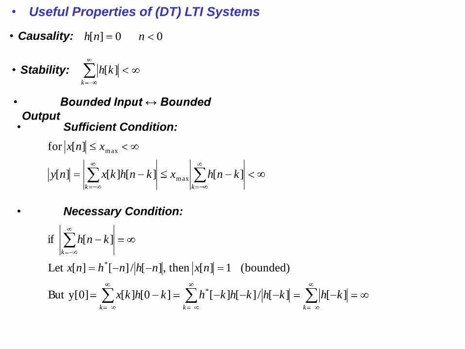
• Useful Properties of (DT) LTI Systems
• Causality:
• Stability:
• Bounded Input ↔ Bounded
Output
00][ nnh
k
kh ][
• Sufficient Condition:
kk
knhxknhkxny
xnx
][][][][
][for
max
max
• Necessary Condition:
kkk
k
khkhkhkhkhkx
nxnhnhnx
knh
][][/][][]0[][y[0]But
(bounded)1][then,][/][][Let
][if
*
*