Embed Size (px)
Citation preview
Outline CT Fourier Transform DT Fourier Transform
Signals and SystemsLecture 5: Fourier Transform
Farzaneh Abdollahi
Department of Electrical Engineering
Amirkabir University of Technology
Winter 2012
Farzaneh Abdollahi Signal and Systems Lecture 5 1/34
Outline CT Fourier Transform DT Fourier Transform
CT Fourier TransformConvergence of CT FTCT FT Properties
DT Fourier TransformConvergence of DT FTDT Fourier Transform for Periodic Signals
DT FT Properties
Farzaneh Abdollahi Signal and Systems Lecture 5 2/34
Outline CT Fourier Transform DT Fourier Transform
CT Fourier Transform
I Fourier series was defined for periodic signals
I Aperiodic signals can be considered as a periodic signal with fundamentalperiod ∞!
I T0 →∞ ω0 → 0I The harmonics get closerI summation (
∑) is substituted by (
∫)
I Fourier series will be replaced by Fourier transform
Farzaneh Abdollahi Signal and Systems Lecture 5 3/34
Outline CT Fourier Transform DT Fourier Transform
Example:
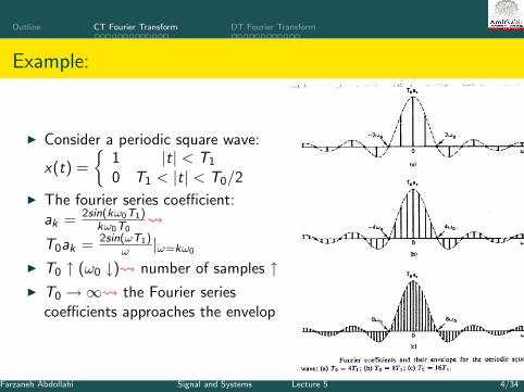
I Consider a periodic square wave:
x(t) =
{1 |t| < T1
0 T1 < |t| < T0/2
I The fourier series coefficient:ak = 2sin(kω0T1)
kω0T0
T0ak = 2sin(ωT1)ω |ω=kω0
I T0 ↑ (ω0 ↓) number of samples ↑I T0 →∞ the Fourier series
coefficients approaches the envelop
Farzaneh Abdollahi Signal and Systems Lecture 5 4/34
Outline CT Fourier Transform DT Fourier Transform
Fourier Transform (FT)
x(t) =1
2π
∫ ∞−∞
X (jω)e jωtdω
X (jω) =
∫ ∞−∞
x(t)e−jωtdt
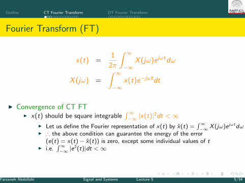
I Convergence of CT FTI x(t) should be square integrable
∫∞−∞ |x(t)|2dt <∞
I Let us define the Fourier representation of x(t) by x̂(t) =∫∞−∞ X (jω)e jωtdω
I ∴ the above condition can guarantee the energy of the error(e(t) = x(t)− x̂(t)) is zero, except some individual values of t
I i.e.∫∞−∞ |e
2(t)|dt <∞
Farzaneh Abdollahi Signal and Systems Lecture 5 5/34
Outline CT Fourier Transform DT Fourier Transform
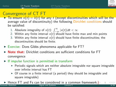
Convergence of CT FTI To ensure x(t) = x̂(t) for any t (except discontinuities which will be the
average value of discontinuity) the following Dirichlet conditions shouldbe satisfied:
1. Absolute integrality of x(t):∫∞−∞ |x(t)|dt <∞
2. Within any finite interval x(t) should have finite max and min points3. Within any finite interval x(t) should have finite discontinuities; the
discontinuities should be finite.
I Exercise: Does Gibbs phenomena applicable for FT?
I Note that: Dirichlet conditions are sufficient conditions for FTconvergence
I If impulse function is permitted in transformI Periodic signals which are neither absolute integrable nor square integrable
over infinite interval has FTI Of course in a finite interval (a period) they should be integrable and
square integrable)
I Hence FT and Fs can be considered in a common framework;)Farzaneh Abdollahi Signal and Systems Lecture 5 6/34
Outline CT Fourier Transform DT Fourier Transform
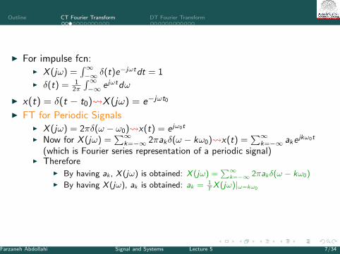
I For impulse fcn:I X (jω) =
∫∞−∞ δ(t)e−jωtdt = 1
I δ(t) = 12π
∫∞−∞ e jωtdω
I x(t) = δ(t − t0) X (jω) = e−jωt0
I FT for Periodic SignalsI X (jω) = 2πδ(ω − ω0) x(t) = e jω0t
I Now for X (jω) =∑∞
k=−∞ 2πakδ(ω − kω0) x(t) =∑∞
k=−∞ akejkω0t
(which is Fourier series representation of a periodic signal)I Therefore
I By having ak , X (jω) is obtained: X (jω) =∑∞
k=−∞ 2πakδ(ω − kω0)I By having X (jω), ak is obtained: ak = 1
TX (jω)|ω=kω0
Farzaneh Abdollahi Signal and Systems Lecture 5 7/34
Outline CT Fourier Transform DT Fourier Transform
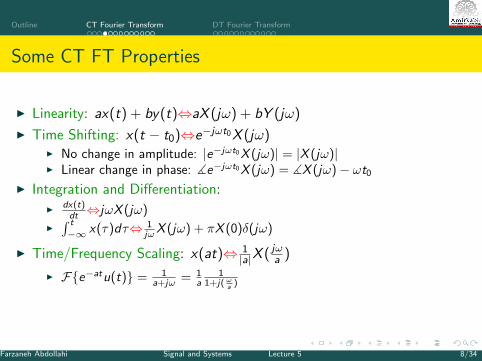
Some CT FT Properties
I Linearity: ax(t) + by(t)⇔aX (jω) + bY (jω)
I Time Shifting: x(t − t0)⇔e−jωt0X (jω)I No change in amplitude: |e−jωt0X (jω)| = |X (jω)|I Linear change in phase: ]e−jωt0X (jω) = ]X (jω)− ωt0
I Integration and Differentiation:I
dx(t)dt ⇔jωX (jω)
I∫ t
−∞ x(τ)dτ⇔ 1jωX (jω) + πX (0)δ(jω)
I Time/Frequency Scaling: x(at)⇔ 1|a|X ( jω
a )
I F{e−atu(t)} = 1a+jω = 1
a1
1+j(ωa )
Farzaneh Abdollahi Signal and Systems Lecture 5 8/34

Outline CT Fourier Transform DT Fourier Transform
I Conjugate and Conjugate Symmetry: x∗(t)⇔X ∗(jω)I Real x(t)⇔X (−jω) = X ∗(jω)
I Polar representation X (jω) = |X (jω)|e j]X (jω)
I|X (−jω)| = |X (jω)| (even fcn)I]X (−jω) = −]X (jω) (odd fcn)
I Rectangular representation X (jω) = Re{X (jω)}+ jIm{X (jω)}IRe{X (−jω)} = Re{X (jω)} (even fcn)IIm{X (−jω)} = −Im{X (jω)} (odd fcn)
I Real and even x(t) = x(−t)⇔X (jω) = X (−jω) = X ∗(jω) (real and evenX (jω))
I Real and odd x(t) = −x(−t)⇔X (−jω) = −X (jω) = −X ∗(jω) (purelyimaginary and odd X (jω)),
I Even part of x(t)⇔Re{X (jω)} (show it!)I Odd part of x(t)⇔jIm{X (jω)} (show it!)
Farzaneh Abdollahi Signal and Systems Lecture 5 9/34
Outline CT Fourier Transform DT Fourier Transform
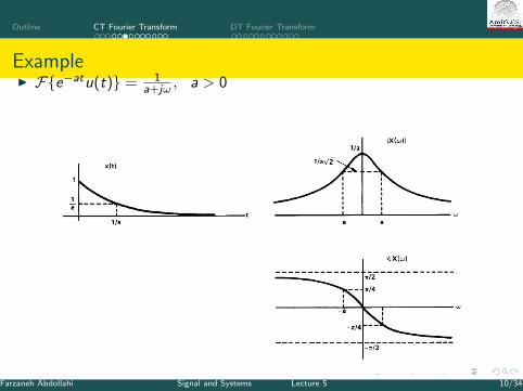
ExampleI F{e−atu(t)} = 1
a+jω , a > 0
Farzaneh Abdollahi Signal and Systems Lecture 5 10/34
Outline CT Fourier Transform DT Fourier Transform
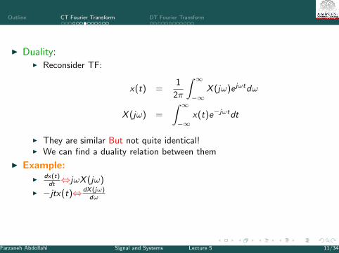
I Duality:I Reconsider TF:
x(t) =1
2π
∫ ∞−∞
X (jω)e jωtdω
X (jω) =
∫ ∞−∞
x(t)e−jωtdt
I They are similar But not quite identical!I We can find a duality relation between them
I Example:I
dx(t)dt ⇔jωX (jω)
I −jtx(t)⇔ dX (jω)dω
Farzaneh Abdollahi Signal and Systems Lecture 5 11/34
Outline CT Fourier Transform DT Fourier Transform
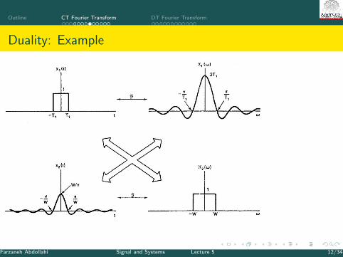
Duality: Example
Farzaneh Abdollahi Signal and Systems Lecture 5 12/34
Outline CT Fourier Transform DT Fourier Transform
Some CT FT Properties
I Parseval’s Relation:∫∞−∞ |x(t)|2dt = 1
2π
∫∞−∞ |X (jω)|2dω
I Total energy in obtained byI computing energy per unit time then integrating over all time ORI computing energy per unit frequency and integrating over all frequencies
I |X (jω)|2 is called energy-density spectrum.
I Convolution: y(t) = x(t) ∗ h(t)⇔Y (jω) = H(jω)X (jω)I This property can be used for filtering input signal in frequency domain.
Farzaneh Abdollahi Signal and Systems Lecture 5 13/34
Outline CT Fourier Transform DT Fourier Transform
FT for LTI Systems
I FT of impulse response, H(jω),is called Frequency Response of thesystem
I Plays a key role in LTI system analyzingI Convergence Condition of FT in LTI Systems
I The LTI system should be stableI i.e., impulse response should be absolute integrable:
∫∞−∞ |h(t)|dt <∞
I Note that this is one of Drichlet’s conditions.I Assume other two Drichlet’s conditions are satisfied (This happens for all
practical systems)I ∴ Only stable LTI systems can be analyzed by FTI Question: How can we analyze unstable LTI systems?
Farzaneh Abdollahi Signal and Systems Lecture 5 14/34
Outline CT Fourier Transform DT Fourier Transform
FT for LTI Systems
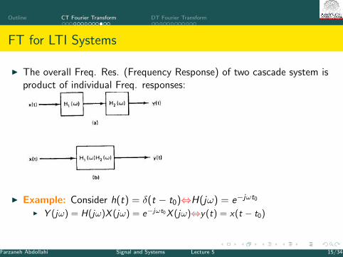
I The overall Freq. Res. (Frequency Response) of two cascade system isproduct of individual Freq. responses:
I Example: Consider h(t) = δ(t − t0)⇔H(jω) = e−jωt0
I Y (jω) = H(jω)X (jω) = e−jωt0X (jω)⇔y(t) = x(t − t0)
Farzaneh Abdollahi Signal and Systems Lecture 5 15/34
Outline CT Fourier Transform DT Fourier Transform
FT for LTI Systems
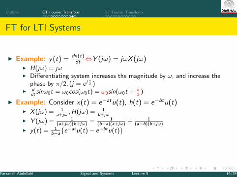
I Example: y(t) = dx(t)dt ⇔Y (jω) = jωX (jω)
I H(jω) = jωI Differentiating system increases the magnitude by ω, and increase the
phase by π/2, (j = e j π2 )I d
dt sinω0t = ω0cos(ω0t) = ω0sin(ω0t + π2 )
I Example: Consider x(t) = e−atu(t), h(t) = e−btu(t)I X (jω) = 1
a+jω ,H(jω) = 1b+jω
I Y (jω) = 1(a+jω)(b+jω) = 1
(b−a)(a+jω) + 1(a−b)(b+jω)
I y(t) = 1b−a{e
−atu(t)− e−btu(t)}
Farzaneh Abdollahi Signal and Systems Lecture 5 16/34

Outline CT Fourier Transform DT Fourier Transform
FT PropertiesI Multiplication: r(t) = s(t)p(t)⇔R(jω) = 1
2π [S(jω) ∗ P(jω)]I Multiplication of two signals is using one signal to scale (modulate) the
amplitude of another one.I ∴ Multiplication of two signals is called amplitude modulation.I Example: p(t) = cos(ω0)t⇔P(jω) = πδ(ω − ω0) + πδ(ω + ω0)
I r(t) = s(t)p(t)⇔R(jω) = 12S(j(ω − ω0)) + 1
2S(j(ω + ω0))
I signal of s(t) is preserved by multiplying it by sinusoidal signal, itsinformation is only shifted to the higher frequency.(sinusoidal amplitudemodulation).
Farzaneh Abdollahi Signal and Systems Lecture 5 17/34
Outline CT Fourier Transform DT Fourier Transform
DT Fourier Transform
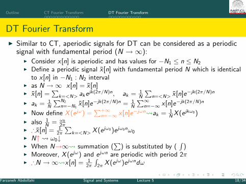
I Similar to CT, aperiodic signals for DT can be considered as a periodicsignal with fundamental period (N →∞):
I Consider x [n] is aperiodic and has values for −N1 ≤ n ≤ N2
I Define a periodic signal x̃ [n] with fundamental period N which is identicalto x [n] in −N1 : N2 interval
I as N →∞ x [n] = x̃ [n]I x̃ [n] =
∑k=<N> ake
jk(2π/N)n, ak = 1N
∑n=<N> x̃ [n]e−jk(2π/N)n
I ak = 1N
∑N2
n=−N1x̃ [n]e−jk(2π/N)n = 1
N
∑∞n=−∞ x [n]e−jk(2π/N)n
I Now define X (e jω) =∑+∞
n=−∞ x [n]e−jωn ak = 1N X (e jkω0)
I also 1N = ω0
2πI ∴x̃ [n] = 1
2π
∑k=<N> X (e jω0)e jω0nω0
I N↑ ω0↓I When N→∞ summation (
∑) is substituted by (
∫)
I Moreover, X (e jω) and e jωn are periodic with period 2πI ∴N →∞ x [n] = 1
2π
∫2π
X (e jω)e jωndω
Farzaneh Abdollahi Signal and Systems Lecture 5 18/34
Outline CT Fourier Transform DT Fourier Transform
DT Fourier Transform
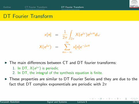
x [n] =1
2π
∫2π
X (e jω)e jωndω
X (e jω) =∞∑
n=−∞x [n]e−jωn
I The main differences between CT and DT fourier transforms:
1. In DT, X (e jω) is periodic2. In DT, the integral of the synthesis equation is finite.
I These properties are similar to DT Fourier Series and they are due to thefact that DT complex exponentials are periodic with 2π
Farzaneh Abdollahi Signal and Systems Lecture 5 19/34
Outline CT Fourier Transform DT Fourier Transform
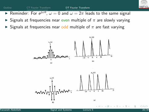
I Reminder: For e jωn, ω = 0 and ω = 2π leads to the same signal
I Signals at frequencies near even multiple of π are slowly varying
I Signals at frequencies near odd multiple of π are fast varying
Farzaneh Abdollahi Signal and Systems Lecture 5 20/34
Outline CT Fourier Transform DT Fourier Transform
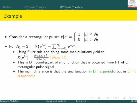
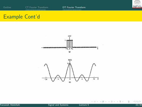
Example
I Consider a rectangular pulse: x [n] =
{1 |n| ≤ N1
0 |n| > N1
I For N1 = 2 : X (e jω) =∑N1
n=−N1e−jωn
I Using Euler rule and doing some manipulations yield to
X (e jω) =sinω(N1+
12 )
sin(ω/2) (Show it!)I This is DT counterpart of sinc function that is obtained from FT of CT
rectangular pulse signalI The main difference is that the sinc function in DT is periodic but in CT it
is aperiodic
Farzaneh Abdollahi Signal and Systems Lecture 5 21/34
Outline CT Fourier Transform DT Fourier Transform
Example Cont’d
Farzaneh Abdollahi Signal and Systems Lecture 5 22/34
Outline CT Fourier Transform DT Fourier Transform
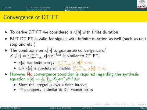
Convergence of DT FT
I To derive DT FT we considered a x [n] with finite duration.
I BUT DT FT is valid for signals with infinite duration as well (such as unitstep and etc.)
I The conditions on x [n] to guarantee convergence ofX (jω) =
∑+∞n=−∞ x [n]e−jωn is similar to CT FT:
I x [n] has finite energy:∑+∞
n=−∞ |x [n]|2 <∞I OR x [n] is absolute summable:
∑+∞n=−∞ |x [n]| <∞
Farzaneh Abdollahi Signal and Systems Lecture 5 23/34
Outline CT Fourier Transform DT Fourier Transform
Convergence of DT FT
I To derive DT FT we considered a x [n] with finite duration.
I BUT DT FT is valid for signals with infinite duration as well (such as unitstep and etc.)
I The conditions on x [n] to guarantee convergence ofX (jω) =
∑+∞n=−∞ x [n]e−jωn is similar to CT FT:
I x [n] has finite energy:∑+∞
n=−∞ |x [n]|2 <∞I OR x [n] is absolute summable:
∑+∞n=−∞ |x [n]| <∞
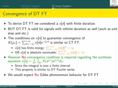
I However No convergence condition is required regarding the synthesisequation x [n] = 1
2π
∫2π X (e jω)e jωndω
I Since the integral is over a finite intervalI This property is similar to DT Fourier series
Farzaneh Abdollahi Signal and Systems Lecture 5 23/34
Outline CT Fourier Transform DT Fourier Transform
Convergence of DT FT
I To derive DT FT we considered a x [n] with finite duration.
I BUT DT FT is valid for signals with infinite duration as well (such as unitstep and etc.)
I The conditions on x [n] to guarantee convergence ofX (jω) =
∑+∞n=−∞ x [n]e−jωn is similar to CT FT:
I x [n] has finite energy:∑+∞
n=−∞ |x [n]|2 <∞I OR x [n] is absolute summable:
∑+∞n=−∞ |x [n]| <∞
I However No convergence condition is required regarding the synthesisequation x [n] = 1
2π
∫2π X (e jω)e jωndω
I Since the integral is over a finite intervalI This property is similar to DT Fourier series
I We would expect No Gibbs phenomenon behavior for DT FT
Farzaneh Abdollahi Signal and Systems Lecture 5 23/34
Outline CT Fourier Transform DT Fourier Transform
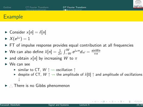
Example
I Consider x [n] = δ[n]
I X (e jω) = 1
I FT of impulse response provides equal contribution at all frequencies
I We can also define x̂ [n] = 12π
∫W−W e jωndω = sinWn
πn
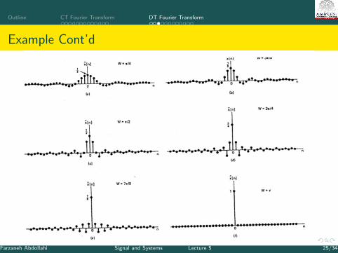
I and obtain x [n] by increasing W to πI We can see
I similar to CT, W ↑ oscillation ↑I despite of CT, W ↑ the amplitude of x̂ [0] ↑ and amplitude of oscillations↓
I ∴ There is no Gibbs phenomenon
Farzaneh Abdollahi Signal and Systems Lecture 5 24/34
Outline CT Fourier Transform DT Fourier Transform
Example Cont’d
Farzaneh Abdollahi Signal and Systems Lecture 5 25/34
Outline CT Fourier Transform DT Fourier Transform
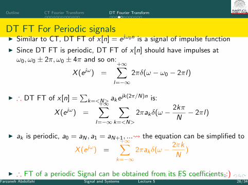
DT FT For Periodic signalsI Similar to CT, DT FT of x [n] = e jω0n is a signal of impulse function
I Since DT FT is periodic, DT FT of x [n] should have impulses atω0, ω0 ± 2π, ω0 ± 4π and so on:
X (e jω) =+∞∑
l=−∞2πδ(ω − ω0 − 2πl)
I ∴ DT FT of x [n] =∑
k=<N> ake jk(2π/N)n is:
X (e jω) =+∞∑
l=−∞
∑k=<N>
2πakδ(ω − 2kπ
N− 2πl)
I ak is periodic, a0 = aN , a1 = aN+1, ... the equation can be simplified to
X (e jω) =+∞∑
k=−∞2πakδ(ω − 2πk
N)
I ∴ FT of a periodic Signal can be obtained from its FS coefficients :)Farzaneh Abdollahi Signal and Systems Lecture 5 26/34
Outline CT Fourier Transform DT Fourier Transform
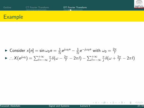
Example
I Consider x [n] = sinω0n = 12j e
jω0n − 12j e−jω0n with ω0 = 2π
7
I ∴ X (e jω0) =∑+∞
l=−∞πj δ(ω − 2π
7 − 2πl)−∑+∞
l=−∞πj δ(ω + 2π
7 − 2πl)
Farzaneh Abdollahi Signal and Systems Lecture 5 27/34
Outline CT Fourier Transform DT Fourier Transform
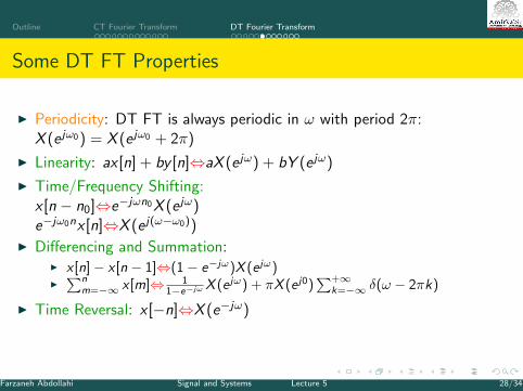
Some DT FT Properties
I Periodicity: DT FT is always periodic in ω with period 2π:X (e jω0) = X (e jω0 + 2π)
I Linearity: ax [n] + by [n]⇔aX (e jω) + bY (e jω)
I Time/Frequency Shifting:x [n − n0]⇔e−jωn0X (e jω)e−jω0nx [n]⇔X (e j(ω−ω0))
I Differencing and Summation:I x [n]− x [n − 1]⇔(1− e−jω)X (e jω)I∑n
m=−∞ x [m]⇔ 11−e−jωX (e jω) + πX (e j0)
∑+∞k=−∞ δ(ω − 2πk)
I Time Reversal: x [−n]⇔X (e−jω)
Farzaneh Abdollahi Signal and Systems Lecture 5 28/34
Outline CT Fourier Transform DT Fourier Transform
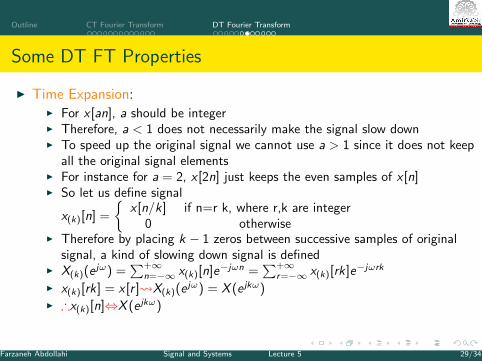
Some DT FT Properties
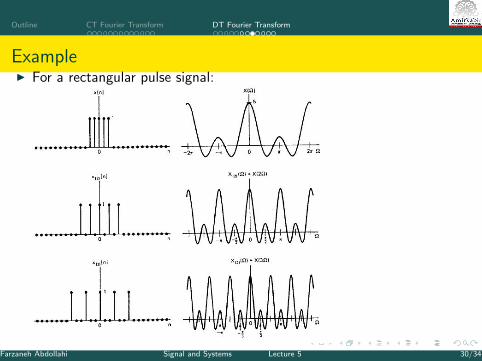
I Time Expansion:I For x [an], a should be integerI Therefore, a < 1 does not necessarily make the signal slow downI To speed up the original signal we cannot use a > 1 since it does not keep
all the original signal elementsI For instance for a = 2, x [2n] just keeps the even samples of x [n]I So let us define signal
x(k)[n] =
{x [n/k] if n=r k, where r,k are integer
0 otherwiseI Therefore by placing k − 1 zeros between successive samples of original
signal, a kind of slowing down signal is definedI X(k)(e
jω) =∑+∞
n=−∞ x(k)[n]e−jωn =∑+∞
r=−∞ x(k)[rk]e−jωrk
I x(k)[rk] = x [r ] X(k)(ejω) = X (e jkω)
I ∴x(k)[n]⇔X (e jkω)
Farzaneh Abdollahi Signal and Systems Lecture 5 29/34
Outline CT Fourier Transform DT Fourier Transform
ExampleI For a rectangular pulse signal:
Farzaneh Abdollahi Signal and Systems Lecture 5 30/34

Outline CT Fourier Transform DT Fourier Transform
I Conjugate and Conjugate Symmetry: x∗[n]⇔X ∗(e−jω)I Real x [n]⇔X (e−jω) = X ∗(e jω)
I Polar representation X (e jω) = |X (e jω)|e j]X (ejω)
I|X (e−jω)| = |X (e jω)| (even fcn)I]X (e−jω) = −]X (e jω) (odd fcn)
I Rectangular representation X (e jω) = Re{X (e jω)}+ jIm{X (e jω)}IRe{X (e−jω)} = Re{X (e jω)} (even fcn)IIm{X (e−jω)} = −Im{X (e jω)} (odd fcn)
I Real and even x [n] = x [−n]⇔X (e jω) = X (e−jω) = X ∗(e jω) (real and evenX (e jω))
I Real and odd x [n] = −x [−n]⇔X (e−jω) = −X (e jω) = −X ∗(e jω) (purelyimaginary and odd X (e jω)),
I even part of x [n]⇔Re{X (e jω)} (show it!)I Odd part of x [n]⇔jIm{X (e jω)} (show it!)
Farzaneh Abdollahi Signal and Systems Lecture 5 31/34
Outline CT Fourier Transform DT Fourier Transform
Some DT FT Properties
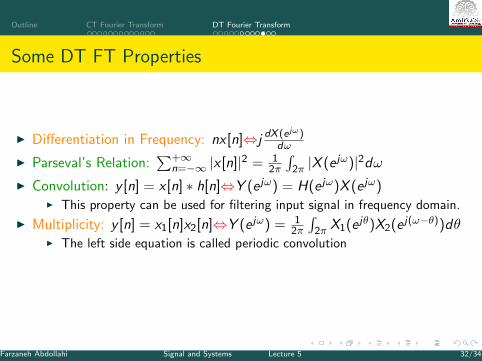
I Differentiation in Frequency: nx [n]⇔j dX (e jω)dω
I Parseval’s Relation:∑+∞
n=−∞ |x [n]|2 = 12π
∫2π |X (e jω)|2dω
I Convolution: y [n] = x [n] ∗ h[n]⇔Y (e jω) = H(e jω)X (e jω)I This property can be used for filtering input signal in frequency domain.
I Multiplicity: y [n] = x1[n]x2[n]⇔Y (e jω) = 12π
∫2π X1(e jθ)X2(e j(ω−θ))dθ
I The left side equation is called periodic convolution
Farzaneh Abdollahi Signal and Systems Lecture 5 32/34
Outline CT Fourier Transform DT Fourier Transform
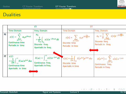
Dualities
Farzaneh Abdollahi Signal and Systems Lecture 5 33/34
Outline CT Fourier Transform DT Fourier Transform
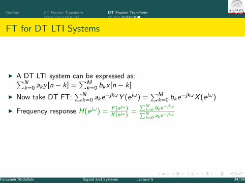
FT for DT LTI Systems
I A DT LTI system can be expressed as:∑Nk=0 aky [n − k] =
∑Mk=0 bkx [n − k]
I Now take DT FT:∑N
k=0 ake−jkωY (e jω) =∑M
k=0 bke−jkωX (e jω)
I Frequency response H(e jω) = Y (e jω)X (e jω)
=∑M
k=0 bke−jkω∑Nk=0 ake−jkω
Farzaneh Abdollahi Signal and Systems Lecture 5 34/34