Signals and Systems

Lecture 2 Wednesday 11th October 2017

DR TANIA STATHAKIREADER (ASSOCIATE PROFFESOR) IN SIGNAL PROCESSINGIMPERIAL COLLEGE LONDON

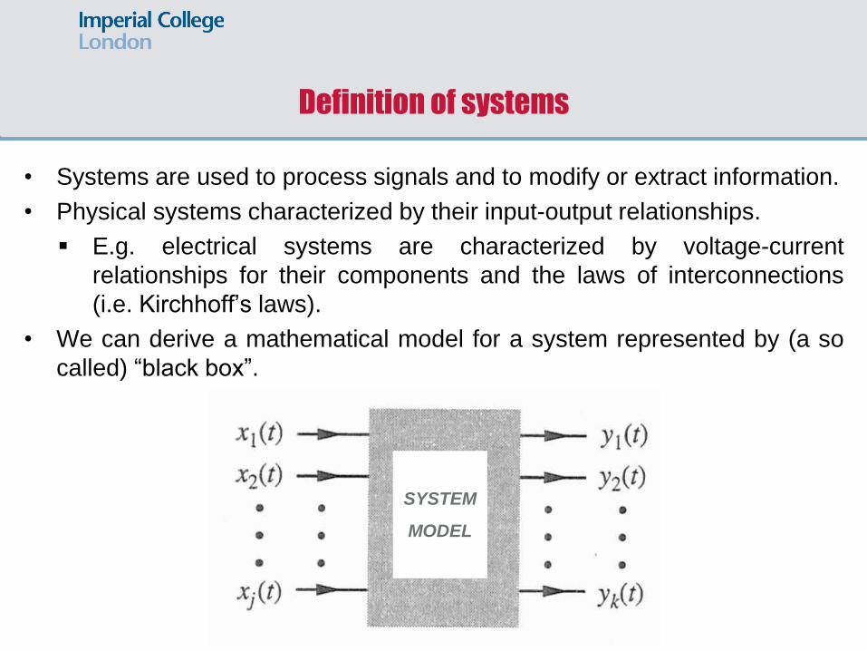
• Systems are used to process signals and to modify or extract information.

• Physical systems characterized by their input-output relationships.

▪ E.g. electrical systems are characterized by voltage-current

relationships for their components and the laws of interconnections

(i.e. Kirchhoff’s laws).

• We can derive a mathematical model for a system represented by (a so

called) “black box”.

SYSTEM

MODEL

Definition of systems

Classification of systems

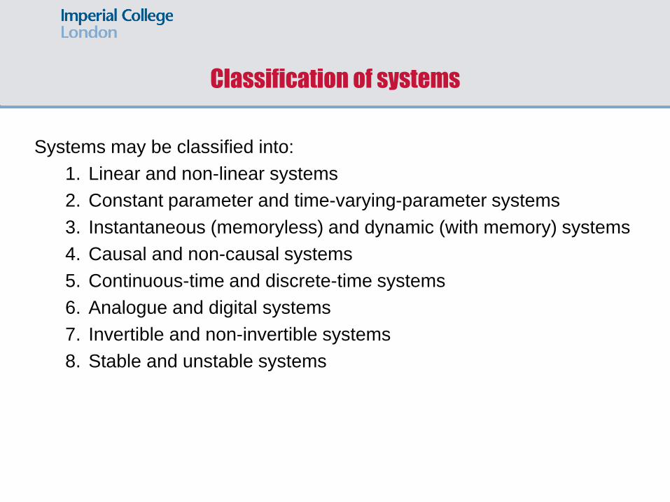
Systems may be classified into:

1. Linear and non-linear systems

2. Constant parameter and time-varying-parameter systems

3. Instantaneous (memoryless) and dynamic (with memory) systems

4. Causal and non-causal systems

5. Continuous-time and discrete-time systems

6. Analogue and digital systems

7. Invertible and non-invertible systems

8. Stable and unstable systems

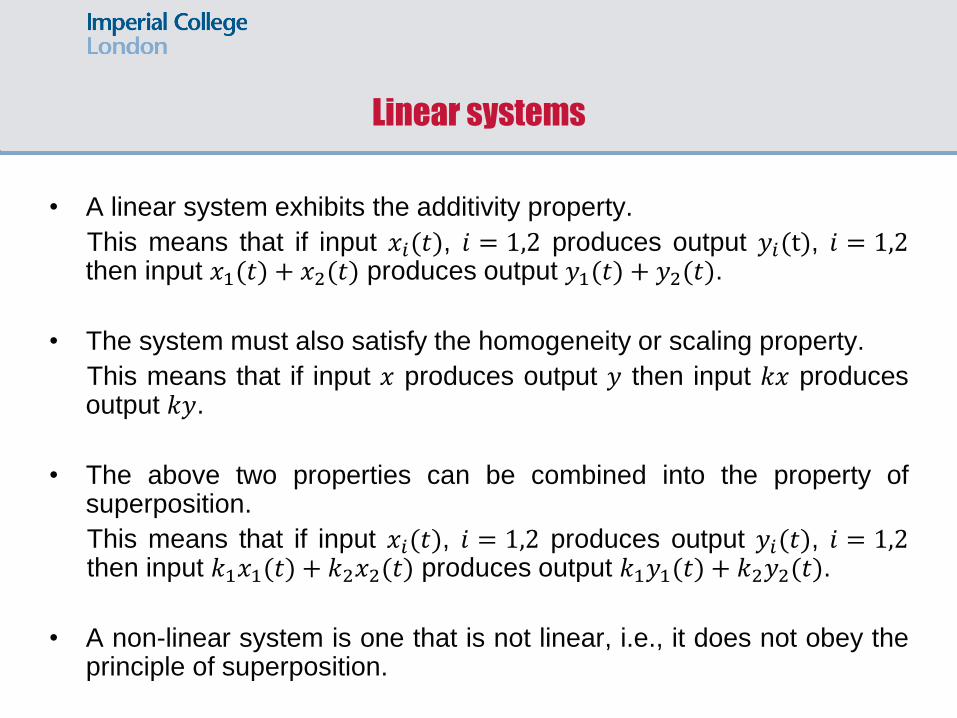
• A linear system exhibits the additivity property.

This means that if input 𝑥𝑖(𝑡), 𝑖 = 1,2 produces output 𝑦𝑖(t), 𝑖 = 1,2then input 𝑥1(𝑡) + 𝑥2(𝑡) produces output 𝑦1(𝑡) + 𝑦2(𝑡).

• The system must also satisfy the homogeneity or scaling property.

This means that if input 𝑥 produces output 𝑦 then input 𝑘𝑥 producesoutput 𝑘𝑦.

• The above two properties can be combined into the property ofsuperposition.

This means that if input 𝑥𝑖(𝑡), 𝑖 = 1,2 produces output 𝑦𝑖(𝑡), 𝑖 = 1,2then input 𝑘1𝑥1(𝑡) + 𝑘2𝑥2(𝑡) produces output 𝑘1𝑦1(𝑡) + 𝑘2𝑦2(𝑡).

• A non-linear system is one that is not linear, i.e., it does not obey theprinciple of superposition.

Linear systems

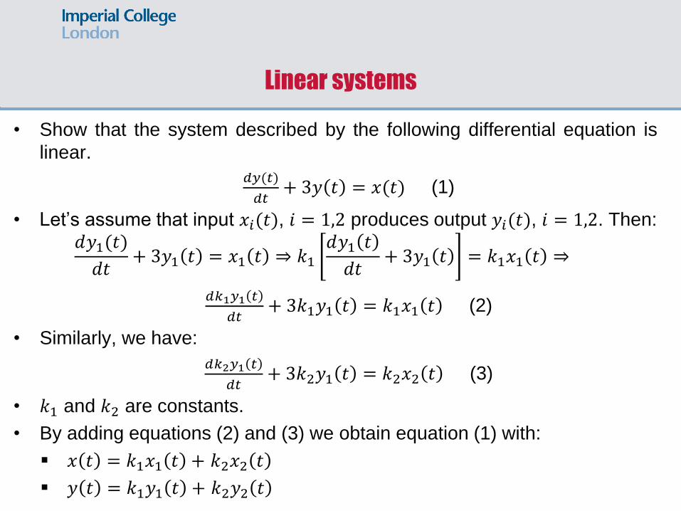
• Show that the system described by the following differential equation is

linear.

𝑑𝑦(𝑡)

𝑑𝑡+ 3𝑦 𝑡 = 𝑥(𝑡) (1)

• Let’s assume that input 𝑥𝑖(𝑡), 𝑖 = 1,2 produces output 𝑦𝑖(𝑡), 𝑖 = 1,2. Then:𝑑𝑦1(𝑡)

𝑑𝑡+ 3𝑦1 𝑡 = 𝑥1 𝑡 ⇒ 𝑘1

𝑑𝑦1 𝑡

𝑑𝑡+ 3𝑦1 𝑡 = 𝑘1𝑥1 𝑡 ⇒

𝑑𝑘1𝑦1 𝑡

𝑑𝑡+ 3𝑘1𝑦1 𝑡 = 𝑘1𝑥1 𝑡 (2)

• Similarly, we have:

𝑑𝑘2𝑦1 𝑡

𝑑𝑡+ 3𝑘2𝑦1 𝑡 = 𝑘2𝑥2 𝑡 (3)

• 𝑘1 and 𝑘2 are constants.

• By adding equations (2) and (3) we obtain equation (1) with:

▪ 𝑥 𝑡 = 𝑘1𝑥1 𝑡 + 𝑘2𝑥2 𝑡

▪ 𝑦 𝑡 = 𝑘1𝑦1 𝑡 + 𝑘2𝑦2 𝑡

Linear systems

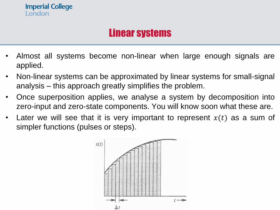
• Almost all systems become non-linear when large enough signals are

applied.

• Non-linear systems can be approximated by linear systems for small-signal

analysis – this approach greatly simplifies the problem.

• Once superposition applies, we analyse a system by decomposition into

zero-input and zero-state components. You will know soon what these are.

• Later we will see that it is very important to represent 𝑥(𝑡) as a sum of

simpler functions (pulses or steps).

Linear systems

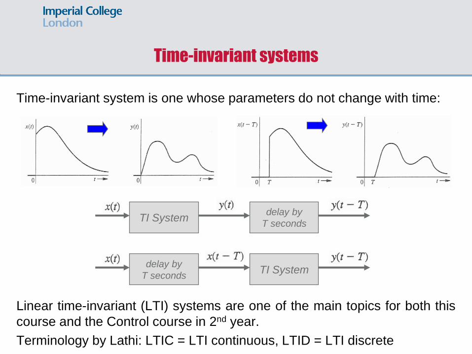
Time-invariant system is one whose parameters do not change with time:

Linear time-invariant (LTI) systems are one of the main topics for both this

course and the Control course in 2nd year.

Terminology by Lathi: LTIC = LTI continuous, LTID = LTI discrete

TI Systemdelay by

T seconds

TI Systemdelay by

T seconds

Time-invariant systems

• In general, a system’s output at time 𝑡 depends on the entire past

input. Such a system is a dynamic (with memory) system.

▪ It is analogous to a state machine in a digital system.

• A system whose response at 𝑡 is completely determined by the input

signals over the past T units of time only is a finite-memory system.

▪ It is analogous to a finite-state machine in a digital system.

• Networks containing inductors and capacitors are infinite memory

dynamic systems.

• If the system’s past history is irrelevant in determining its response, it is

an instantaneous or memoryless system.

▪ This is analogous to a combinatorial circuit in a digital system.

Instantaneous and dynamic Systems

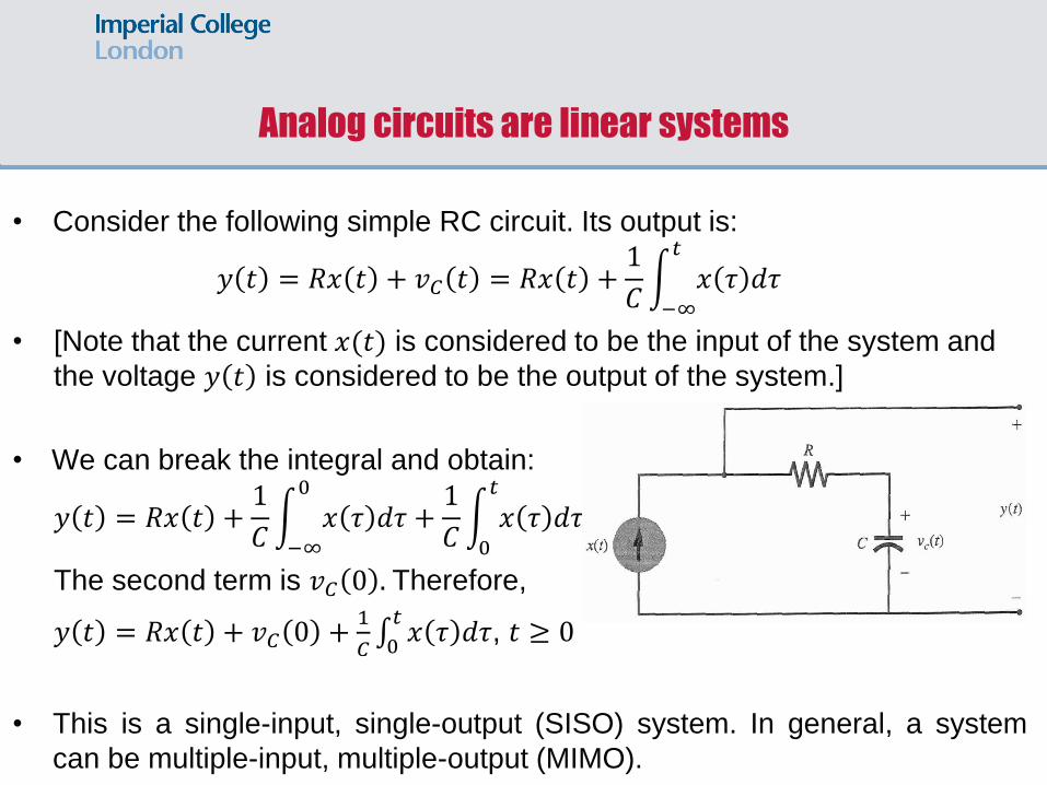
• Consider the following simple RC circuit. Its output is:

𝑦 𝑡 = 𝑅𝑥 𝑡 + 𝑣𝐶 𝑡 = 𝑅𝑥 𝑡 +1

𝐶න−∞

𝑡

𝑥 𝜏 𝑑𝜏

• [Note that the current 𝑥(𝑡) is considered to be the input of the system and

the voltage 𝑦 𝑡 is considered to be the output of the system.]

• We can break the integral and obtain:

𝑦 𝑡 = 𝑅𝑥 𝑡 +1

𝐶න−∞

0

𝑥 𝜏 𝑑𝜏 +1

𝐶න0

𝑡

𝑥 𝜏 𝑑𝜏

The second term is 𝑣𝐶 0 . Therefore,

𝑦 𝑡 = 𝑅𝑥 𝑡 + 𝑣𝐶 0 +1

𝐶0𝑡𝑥 𝜏 𝑑𝜏, 𝑡 ≥ 0

• This is a single-input, single-output (SISO) system. In general, a system

can be multiple-input, multiple-output (MIMO).

Analog circuits are linear systems

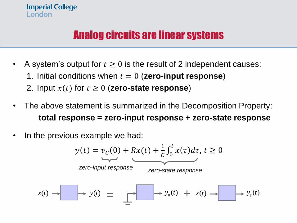
• A system’s output for 𝑡 ≥ 0 is the result of 2 independent causes:

1. Initial conditions when 𝑡 = 0 (zero-input response)

2. Input 𝑥(𝑡) for 𝑡 ≥ 0 (zero-state response)

• The above statement is summarized in the Decomposition Property:

total response = zero-input response + zero-state response

• In the previous example we had:

𝑦 𝑡 = 𝑣𝐶 0 + 𝑅𝑥(𝑡) +1

𝐶0𝑡𝑥 𝜏 𝑑𝜏, 𝑡 ≥ 0

zero-input response zero-state response

( )x t ( )y t ( )x t ( )sy t0 ( )y t +=

Analog circuits are linear systems

• In a causal system the output at 𝑡0 depends only on 𝑥 𝑡 , 𝑡 ≤ 𝑡0.

• The above statement implies that the present output depends only on

the past and present inputs, not on future inputs.

• Any practical real-time system must be causal.

• Non-causal systems are also important because:

1. The can still be realizable when the independent variable is

something other than “time” (e.g. space).

2. For temporal systems, as for example video, we can pre-record the

data and process them in a non-real time fashion. In that case the

systems will be non-causal.

Causal and non-causal systems

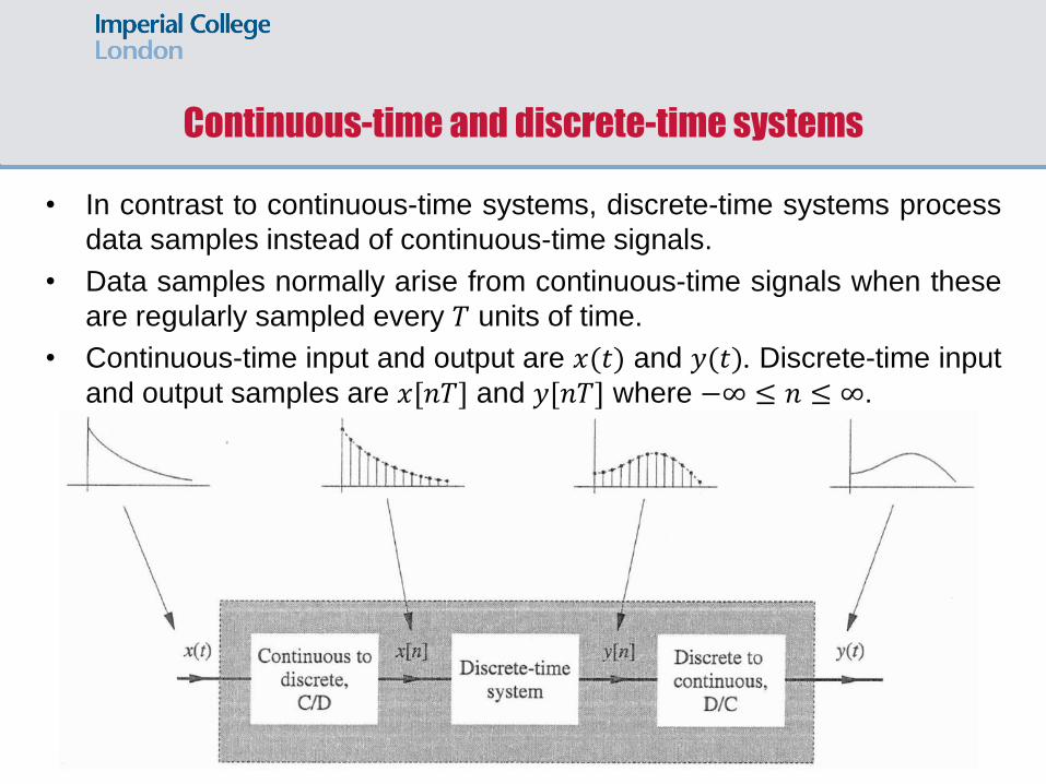
• In contrast to continuous-time systems, discrete-time systems process

data samples instead of continuous-time signals.

• Data samples normally arise from continuous-time signals when these

are regularly sampled every 𝑇 units of time.

• Continuous-time input and output are 𝑥(𝑡) and 𝑦(𝑡). Discrete-time input

and output samples are 𝑥[𝑛𝑇] and 𝑦[𝑛𝑇] where −∞ ≤ 𝑛 ≤ ∞.

Continuous-time and discrete-time systems

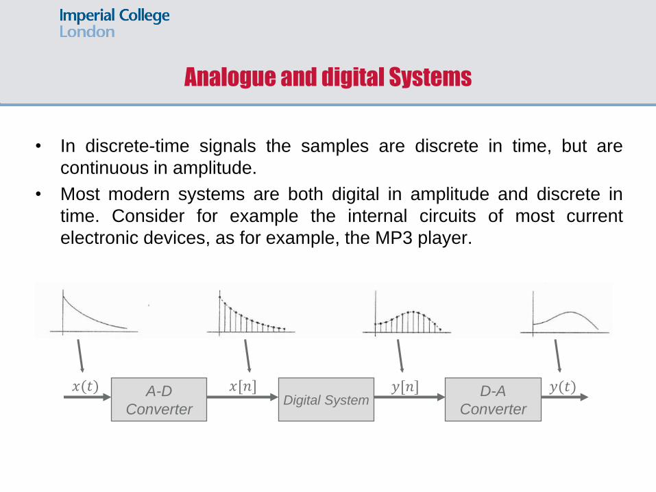
• In discrete-time signals the samples are discrete in time, but are

continuous in amplitude.

• Most modern systems are both digital in amplitude and discrete in

time. Consider for example the internal circuits of most current

electronic devices, as for example, the MP3 player.

A-D

ConverterDigital System

D-A

Converter

𝑥(𝑡) 𝑥[𝑛] 𝑦[𝑛] 𝑦(𝑡)

Analogue and digital Systems

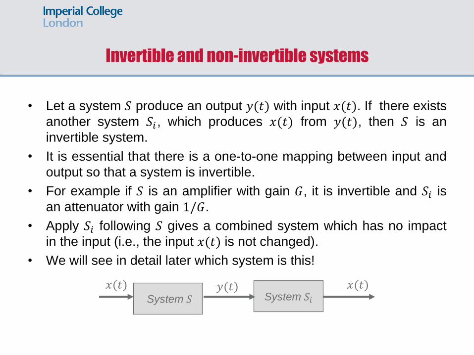
• Let a system 𝑆 produce an output 𝑦(𝑡) with input 𝑥(𝑡). If there exists

another system 𝑆𝑖 , which produces 𝑥(𝑡) from 𝑦(𝑡), then 𝑆 is an

invertible system.

• It is essential that there is a one-to-one mapping between input and

output so that a system is invertible.

• For example if 𝑆 is an amplifier with gain 𝐺, it is invertible and 𝑆𝑖 is

an attenuator with gain 1/𝐺.

• Apply 𝑆𝑖 following 𝑆 gives a combined system which has no impact

in the input (i.e., the input 𝑥(𝑡) is not changed).

• We will see in detail later which system is this!

System 𝑆𝑖System 𝑆

𝑥(𝑡) 𝑥(𝑡)𝑦(𝑡)

Invertible and non-invertible systems

• Externally stable systems are the ones in which a bounded input

results in a bounded output (the system is said to be stable in the

BIBO sense).

• Stability of a system will be discussed after introducing Fourier and

Laplace transforms.

• More detailed analysis of stability is covered in the Control course.

Stable and unstable systems

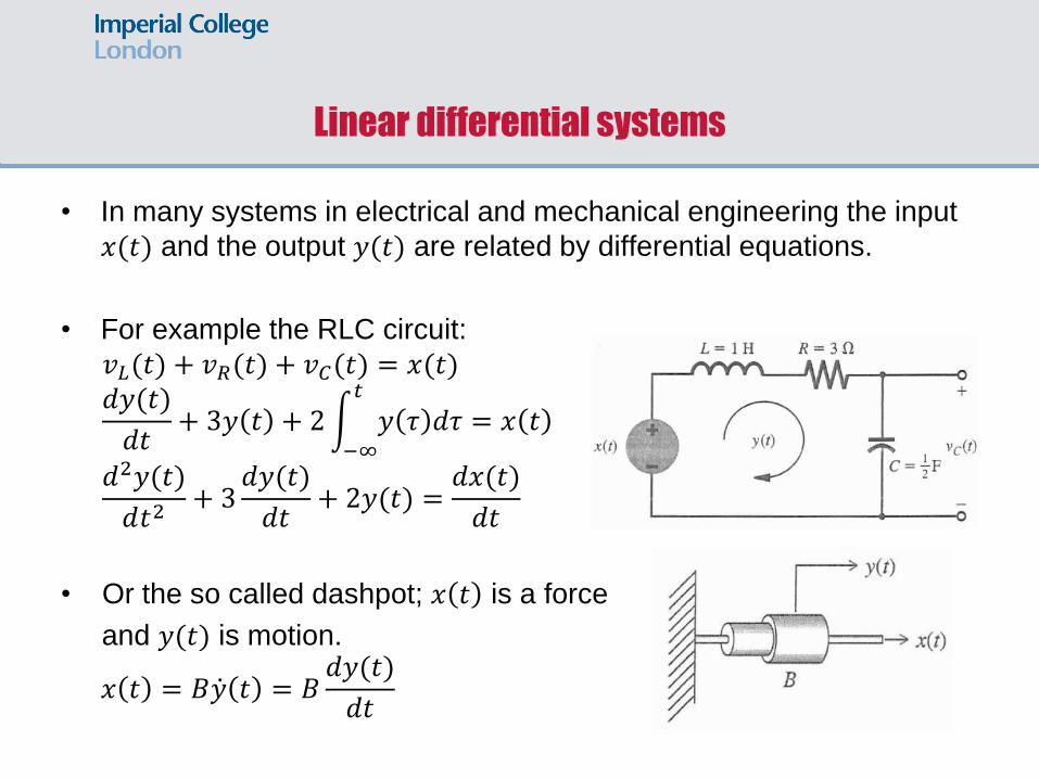
• In many systems in electrical and mechanical engineering the input

𝑥(𝑡) and the output 𝑦(𝑡) are related by differential equations.

• For example the RLC circuit:

𝑣𝐿(𝑡) + 𝑣𝑅(𝑡) + 𝑣𝐶(𝑡) = 𝑥(𝑡)𝑑𝑦(𝑡)

𝑑𝑡+ 3𝑦 𝑡 + 2න

−∞

𝑡

𝑦 𝜏 𝑑𝜏 = 𝑥 𝑡

𝑑2𝑦(𝑡)

𝑑𝑡2+ 3

𝑑𝑦(𝑡)

𝑑𝑡+ 2𝑦(𝑡) =

𝑑𝑥(𝑡)

𝑑𝑡

• Or the so called dashpot; 𝑥 𝑡 is a force

and 𝑦(𝑡) is motion.

𝑥 𝑡 = 𝐵 ሶ𝑦 𝑡 = 𝐵𝑑𝑦(𝑡)

𝑑𝑡

Linear differential systems

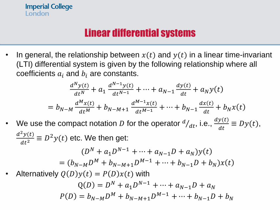
• In general, the relationship between 𝑥(𝑡) and 𝑦(𝑡) in a linear time-invariant

(LTI) differential system is given by the following relationship where all

coefficients 𝑎𝑖 and 𝑏𝑖 are constants.

𝑑𝑁𝑦(𝑡)

𝑑𝑡𝑁+ 𝑎1

𝑑𝑁−1𝑦(𝑡)

𝑑𝑡𝑁−1+⋯+ 𝑎𝑁−1

𝑑𝑦 𝑡

𝑑𝑡+ 𝑎𝑁𝑦 𝑡

= 𝑏𝑁−𝑀𝑑𝑀𝑥(𝑡)

𝑑𝑡𝑀+ 𝑏𝑁−𝑀+1

𝑑𝑀−1𝑥(𝑡)

𝑑𝑡𝑀−1 +⋯+ 𝑏𝑁−1𝑑𝑥 𝑡

𝑑𝑡+ 𝑏𝑁𝑥 𝑡

• We use the compact notation 𝐷 for the operator Τ𝑑 𝑑𝑡, i.e., 𝑑𝑦(𝑡)

𝑑𝑡≡ 𝐷𝑦(𝑡),

𝑑2𝑦(𝑡)

𝑑𝑡2≡ 𝐷2𝑦(𝑡) etc. We then get:

(𝐷𝑁 + 𝑎1𝐷𝑁−1 +⋯+ 𝑎𝑁−1𝐷 + 𝑎𝑁)𝑦 𝑡

= (𝑏𝑁−𝑀𝐷𝑀 + 𝑏𝑁−𝑀+1𝐷

𝑀−1 +⋯+ 𝑏𝑁−1𝐷 + 𝑏𝑁)𝑥 𝑡

• Alternatively 𝑄 𝐷 𝑦 𝑡 = 𝑃 𝐷 𝑥(𝑡) with

Q 𝐷 = 𝐷𝑁 + 𝑎1𝐷𝑁−1 +⋯+ 𝑎𝑁−1𝐷 + 𝑎𝑁

𝑃 𝐷 = 𝑏𝑁−𝑀𝐷𝑀 + 𝑏𝑁−𝑀+1𝐷

𝑀−1 +⋯+ 𝑏𝑁−1𝐷 + 𝑏𝑁

Linear differential systems

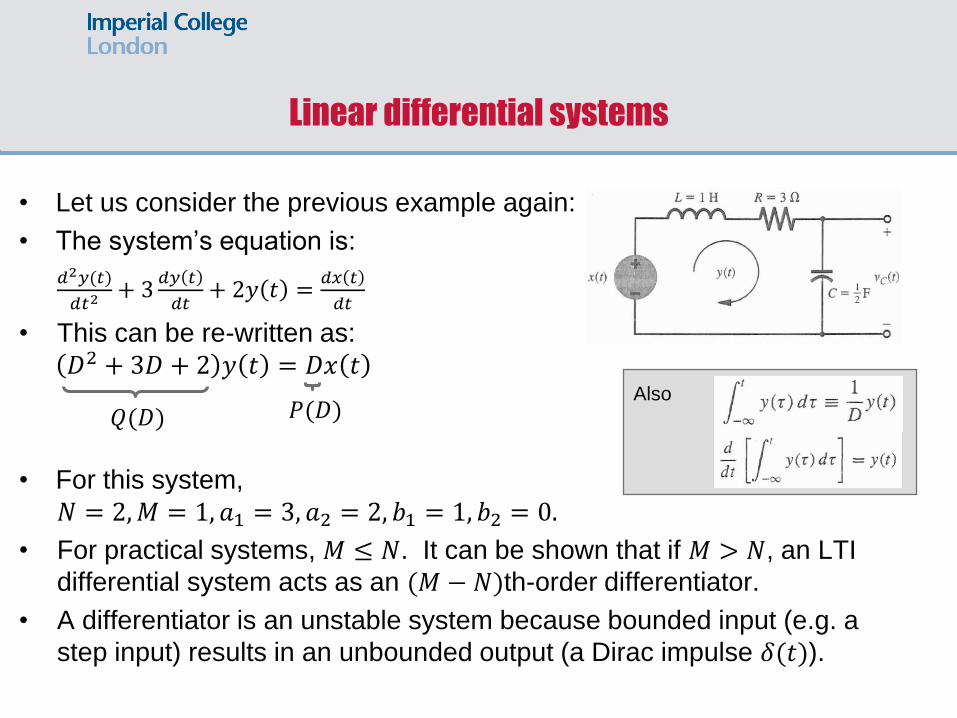
• Let us consider the previous example again:

• The system’s equation is:

𝑑2𝑦(𝑡)

𝑑𝑡2+ 3

𝑑𝑦 𝑡

𝑑𝑡+ 2𝑦 𝑡 =

𝑑𝑥 𝑡

𝑑𝑡

• This can be re-written as:

𝐷2 + 3𝐷 + 2 𝑦 𝑡 = 𝐷𝑥 𝑡

• For this system,

𝑁 = 2,𝑀 = 1, 𝑎1 = 3, 𝑎2 = 2, 𝑏1 = 1, 𝑏2 = 0.

• For practical systems, 𝑀 ≤ 𝑁. It can be shown that if 𝑀 > 𝑁, an LTI

differential system acts as an (𝑀 − 𝑁)th-order differentiator.

• A differentiator is an unstable system because bounded input (e.g. a

step input) results in an unbounded output (a Dirac impulse 𝛿(𝑡)).

Also

𝑄(𝐷) 𝑃(𝐷)

Linear differential systems

• The principle of superposition and circuit analysis using differential

equations was taught in 1st year circuit courses.

▪ Key conceptual difference: the problem is now tackled from a “black

box” approach.

• System modelling is the key not only for the analysis of circuits, but other

types of systems as well (financial, mechanical and others).

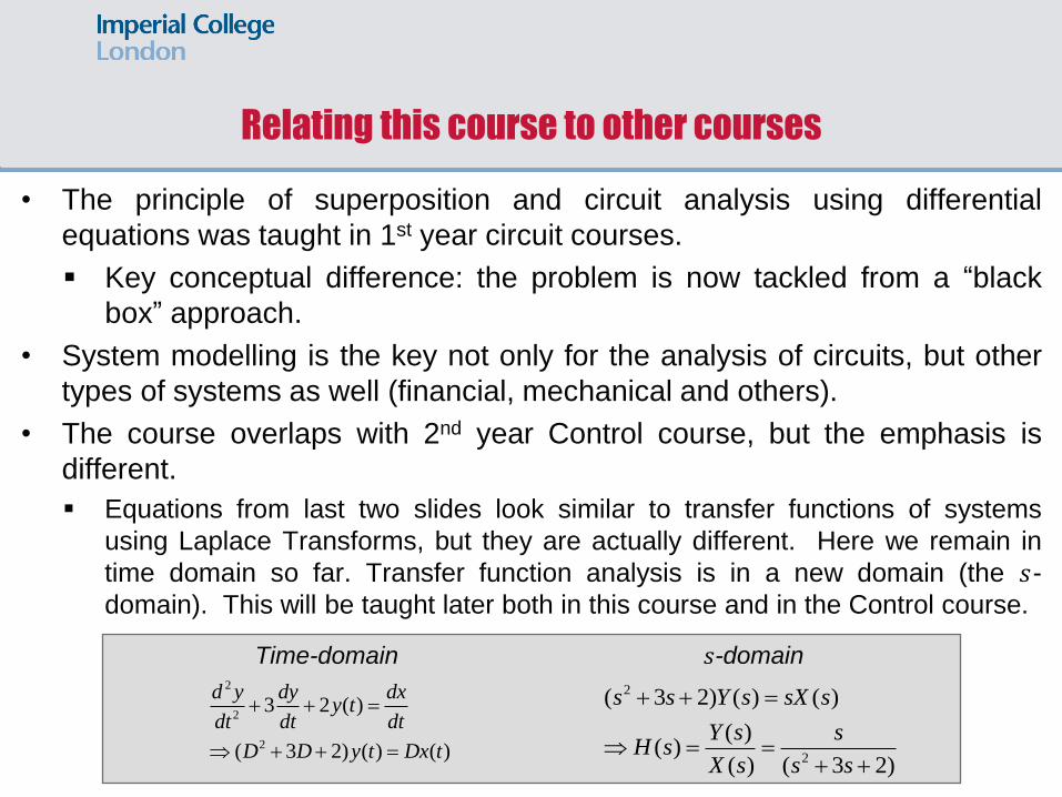
• The course overlaps with 2nd year Control course, but the emphasis is

different.

▪ Equations from last two slides look similar to transfer functions of systems

using Laplace Transforms, but they are actually different. Here we remain in

time domain so far. Transfer function analysis is in a new domain (the 𝑠-

domain). This will be taught later both in this course and in the Control course.

2

2

2

3 2 ( )

( 3 2) ( ) ( )

d y dy dxy t

dt dt dt

D D y t Dx t

Time-domain

2

2

( 3 2) ( ) ( )

( )( )

( ) ( 3 2)

s s Y s sX s

Y s sH s

X s s s

𝑠-domain

Relating this course to other courses