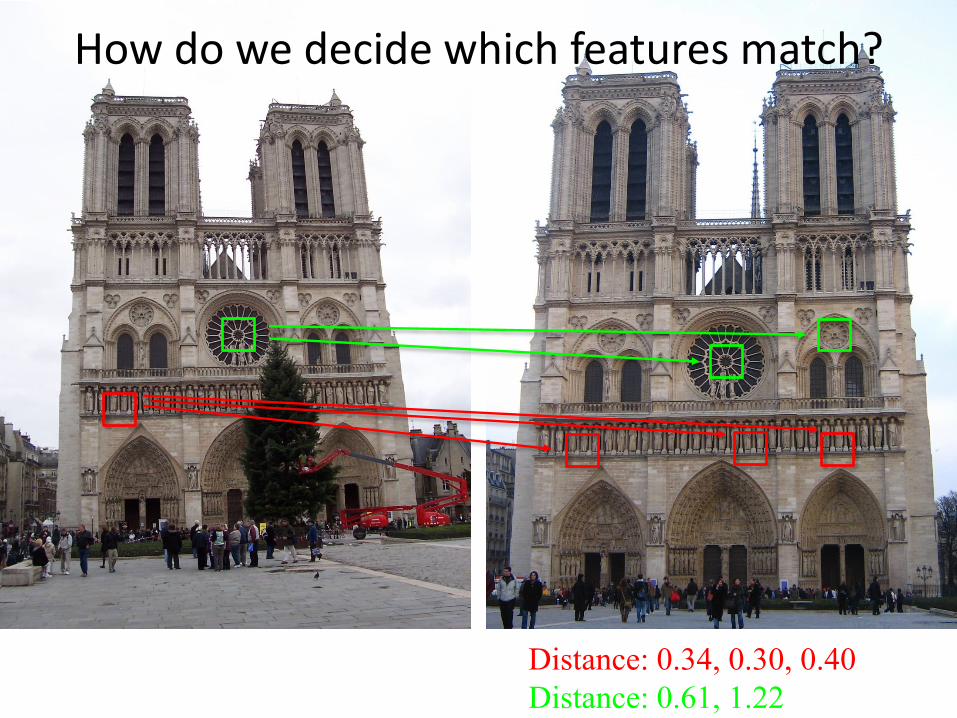
Distance: 0.34, 0.30, 0.40

Distance: 0.61, 1.22

How do we decide which features match?

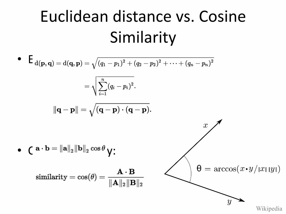
Euclidean distance vs. Cosine Similarity

• Euclidean distance:

• Cosine similarity:

Wikipedia

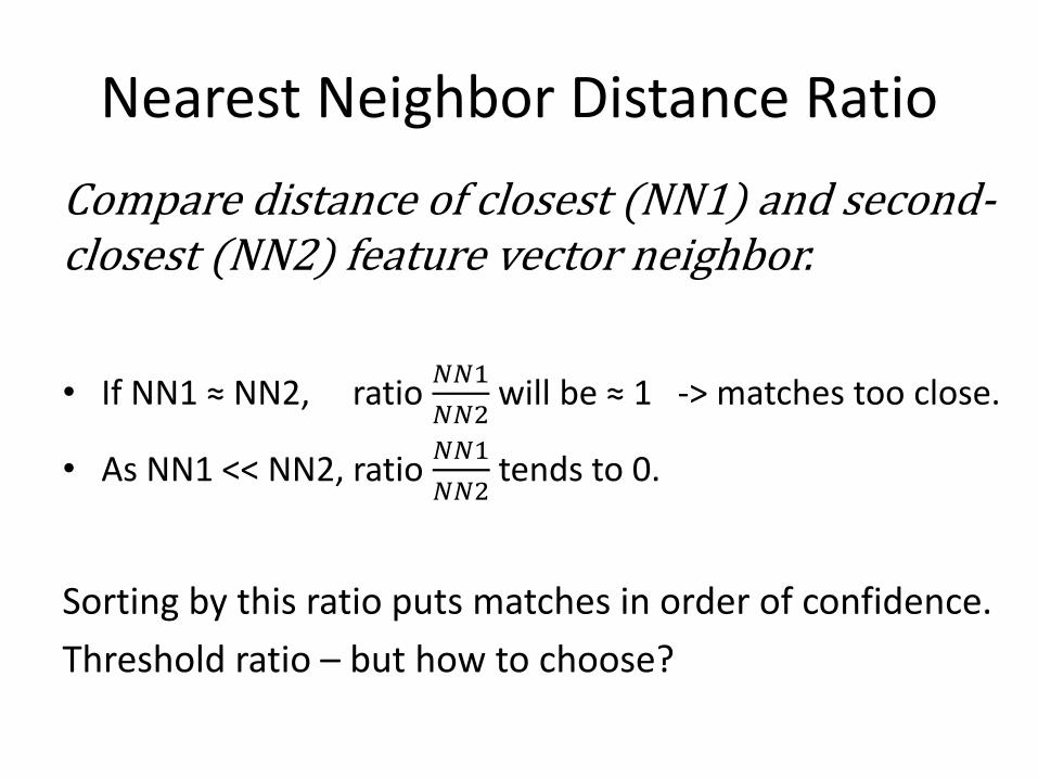
Nearest Neighbor Distance Ratio

Compare distance of closest (NN1) and second-closest (NN2) feature vector neighbor.

• If NN1 ≈ NN2, ratio 𝑁𝑁1

𝑁𝑁2will be ≈ 1 -> matches too close.

• As NN1 << NN2, ratio 𝑁𝑁1

𝑁𝑁2tends to 0.

Sorting by this ratio puts matches in order of confidence.

Threshold ratio – but how to choose?

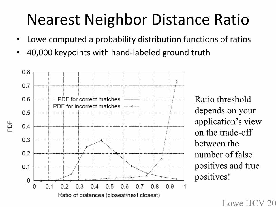
Nearest Neighbor Distance Ratio• Lowe computed a probability distribution functions of ratios

• 40,000 keypoints with hand-labeled ground truth

Lowe IJCV 2004

Ratio threshold

depends on your

application’s view

on the trade-off

between the

number of false

positives and true

positives!

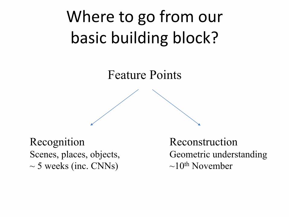
Where to go from our basic building block?

Feature Points

ReconstructionGeometric understanding

~10th November

RecognitionScenes, places, objects,

~ 5 weeks (inc. CNNs)

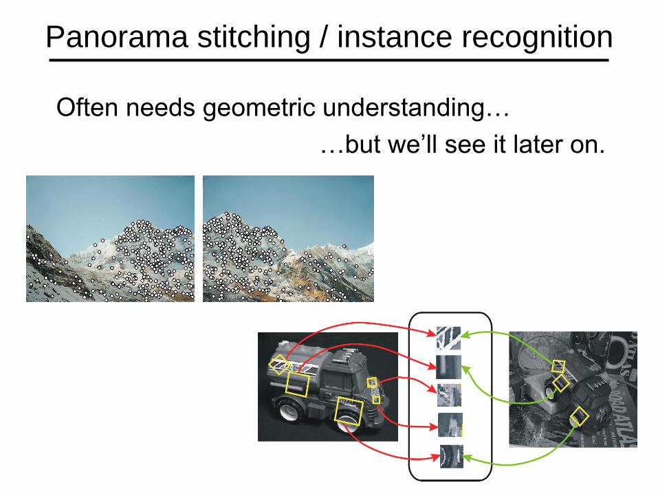
Panorama stitching / instance recognition

Often needs geometric understanding…

…but we’ll see it later on.

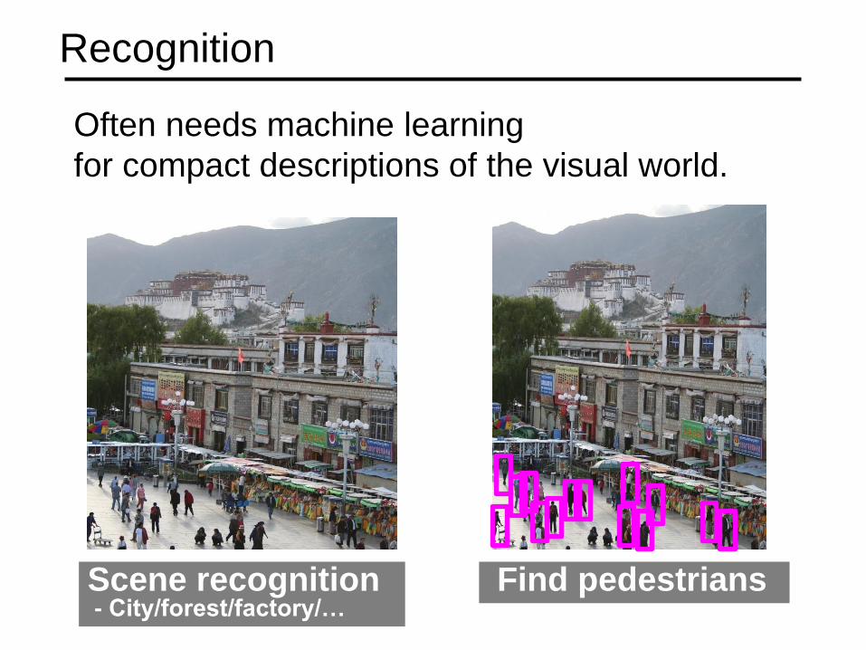
Recognition

Often needs machine learning

for compact descriptions of the visual world.

Scene recognition- City/forest/factory/…

Find pedestrians

ML CRASH COURSE

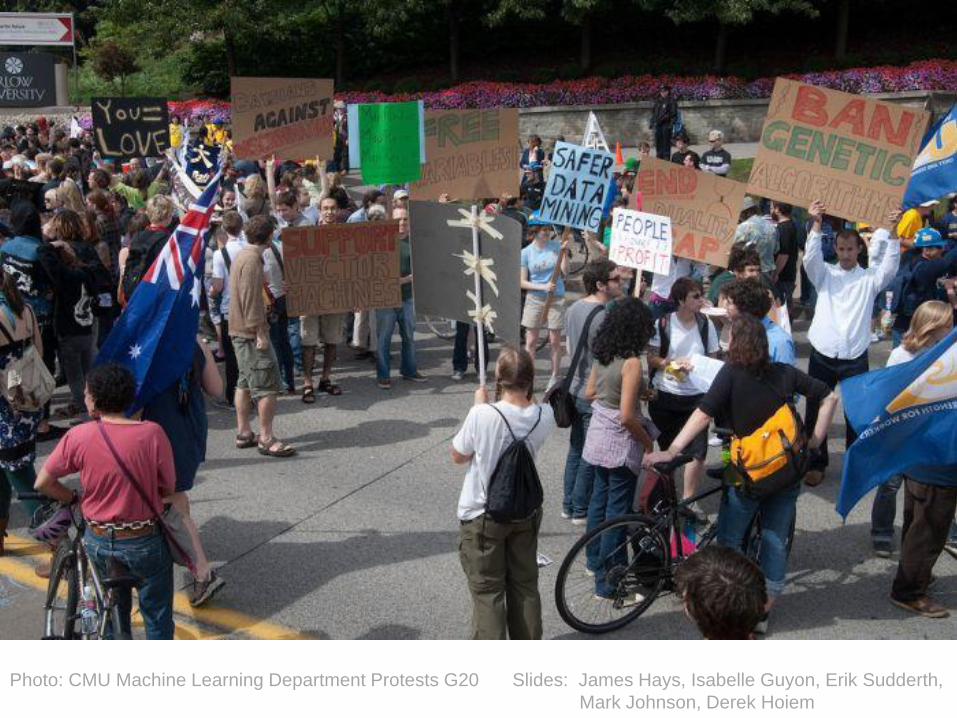
Slides: James Hays, Isabelle Guyon, Erik Sudderth,

Mark Johnson, Derek Hoiem

Photo: CMU Machine Learning Department Protests G20

Slides: James Hays, Isabelle Guyon, Erik Sudderth,

Mark Johnson, Derek Hoiem

Photo: CMU Machine Learning Department Protests G20

Our approach

• We will look at ML as a tool. We will not detail the underpinnings of each learning method.

• Please take a machine learning course if you want to know more!

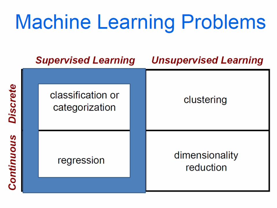
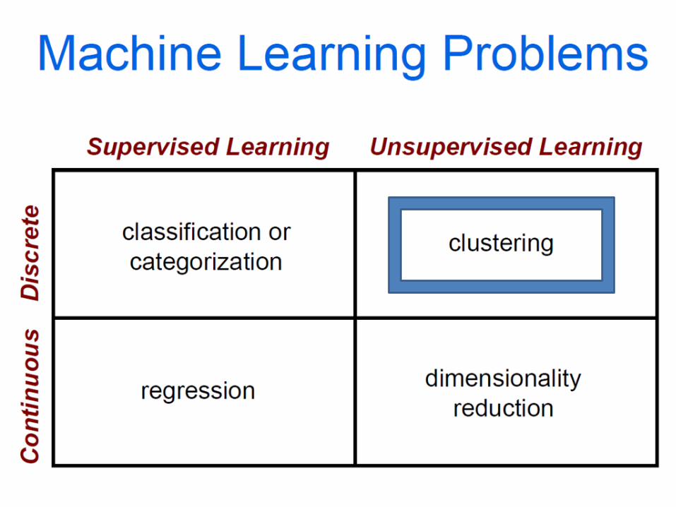
Machine Learning

• Learn from and make predictions on data.

• Arguably the greatest export from computing to other scientific fields.

• Statisticians might disagree with CompScis on the true origins…

ML for Computer Vision

• Face Recognition

• Object Classification

• Scene Segmentation

Data, data, data!

• Norvig – “The Unreasonable Effectiveness of Data” (IEEE Intelligent Systems, 2009)

– “... invariably, simple models and a lot of data trump more elaborate models based on less data”

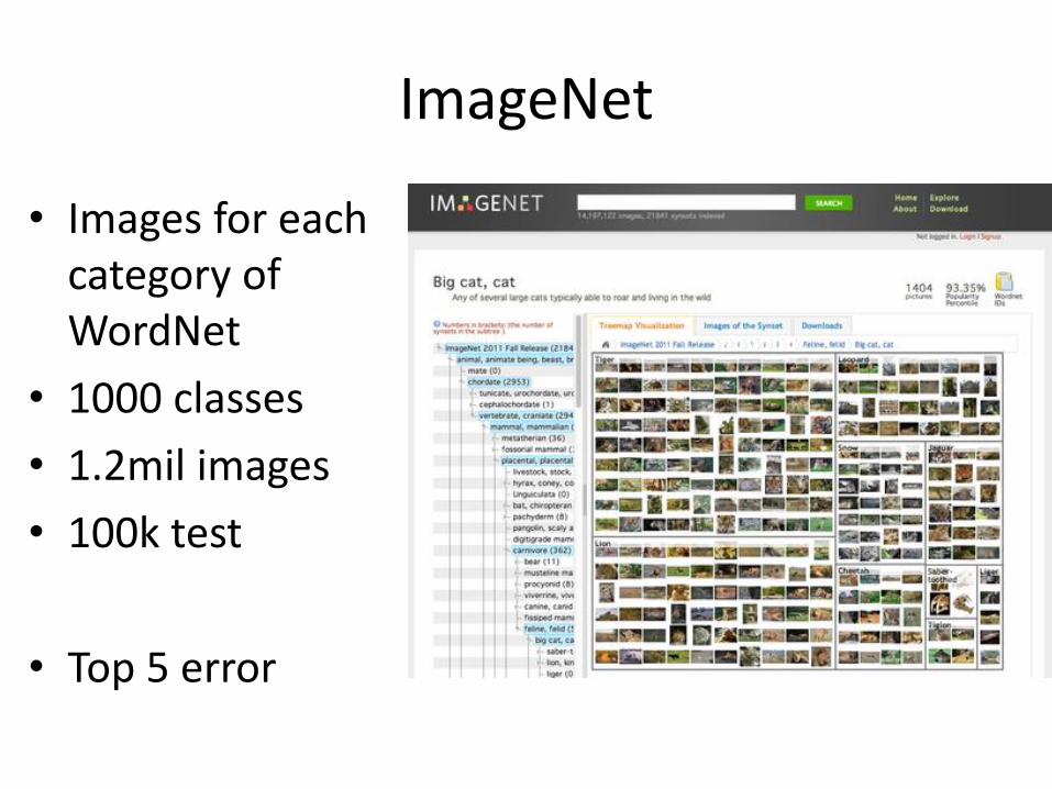
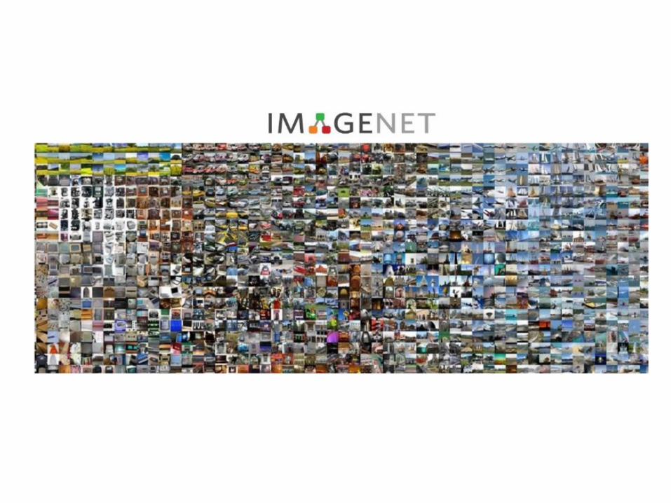
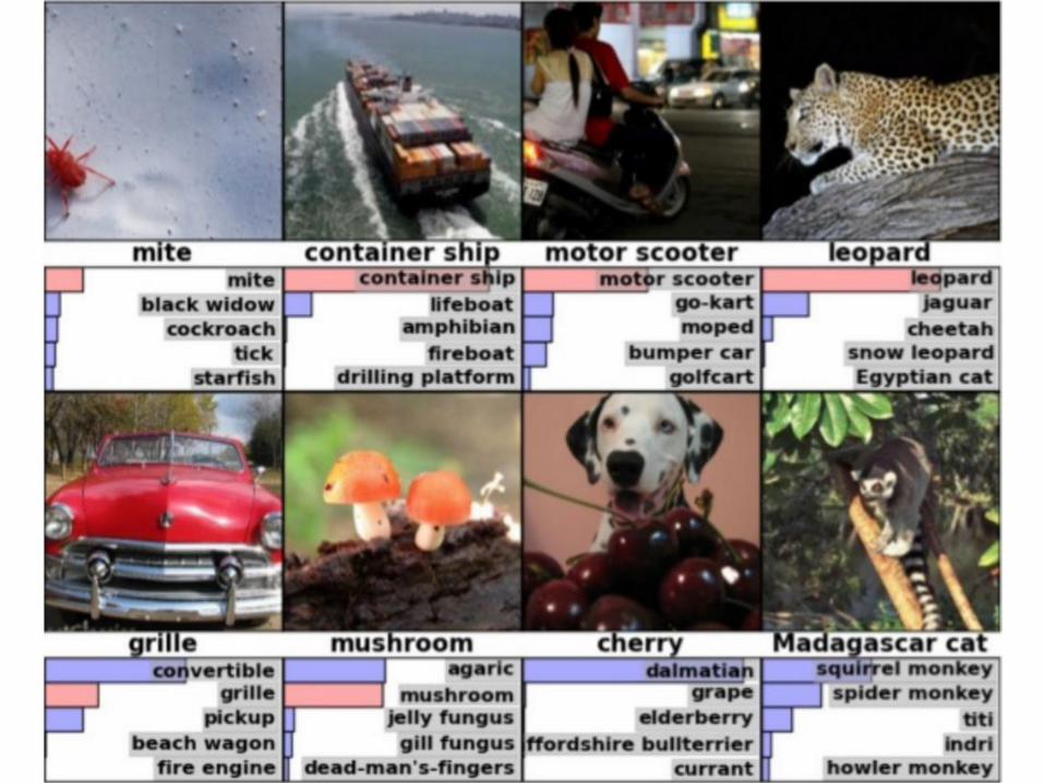
ImageNet

• Images for each category of WordNet

• 1000 classes

• 1.2mil images

• 100k test

• Top 5 error

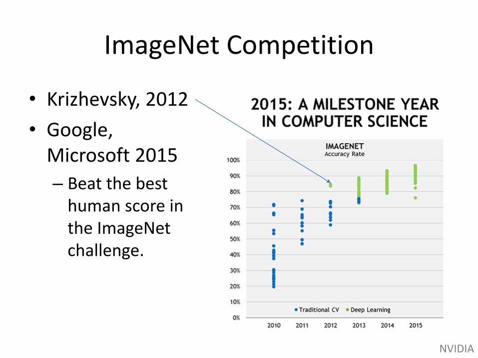
ImageNet Competition

• Krizhevsky, 2012

• Google, Microsoft 2015

– Beat the best human score in the ImageNet challenge.

NVIDIA

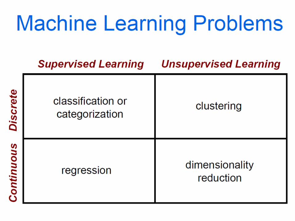
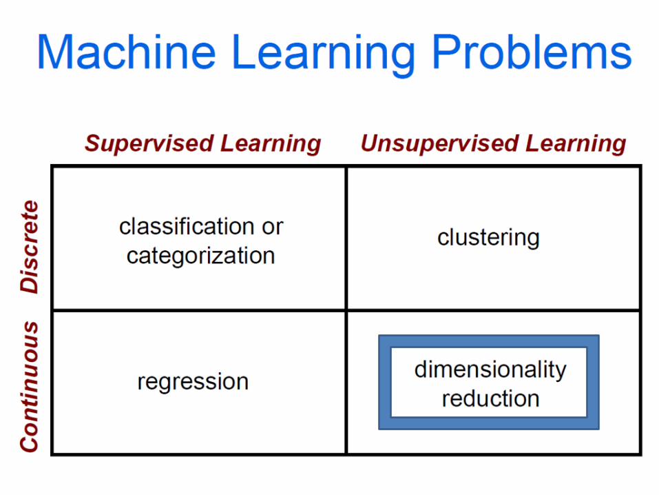
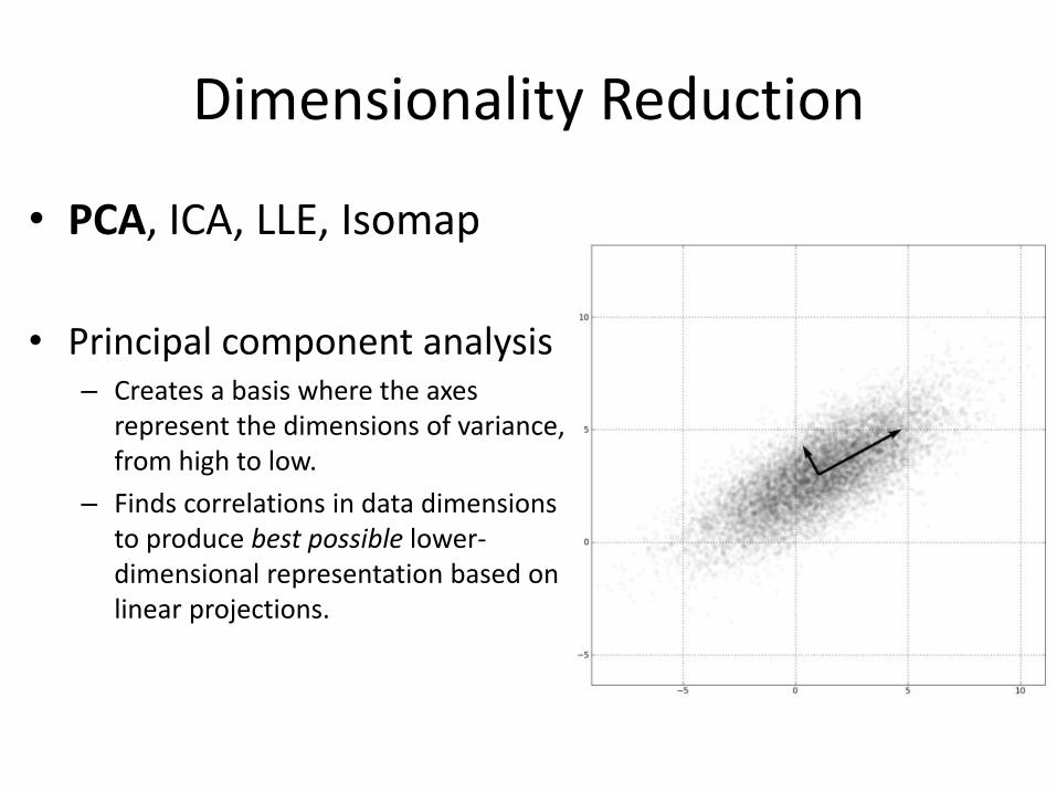
Dimensionality Reduction

• PCA, ICA, LLE, Isomap

• Principal component analysis– Creates a basis where the axes

represent the dimensions of variance, from high to low.

– Finds correlations in data dimensions to produce best possible lower-dimensional representation based on linear projections.

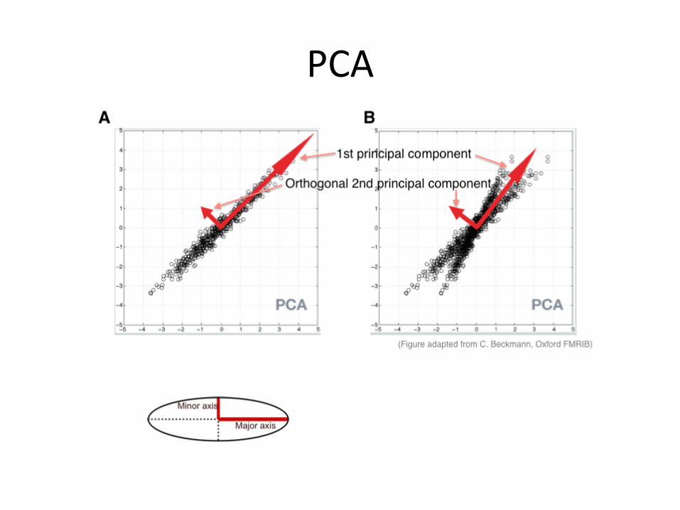
PCA

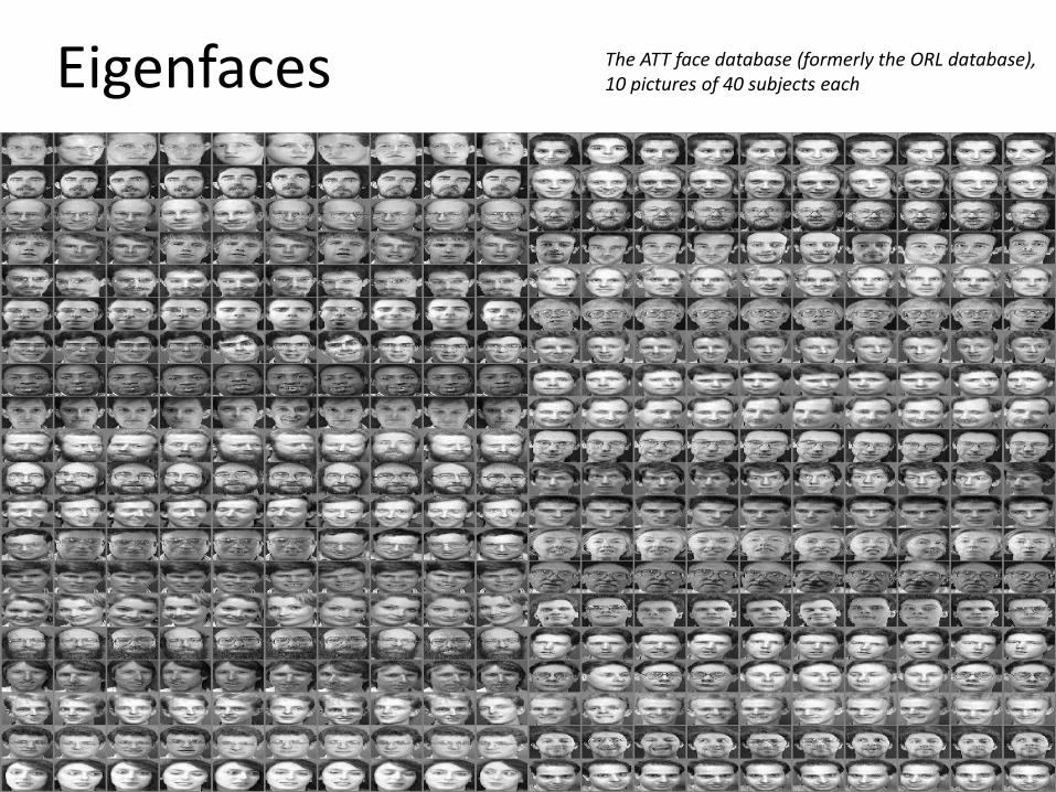
Eigenfaces The ATT face database (formerly the ORL database), 10 pictures of 40 subjects each

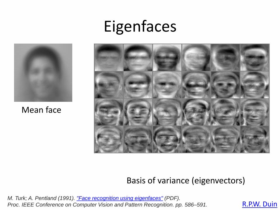
Eigenfaces

M. Turk; A. Pentland (1991). "Face recognition using eigenfaces" (PDF).

Proc. IEEE Conference on Computer Vision and Pattern Recognition. pp. 586–591.

Mean face

Basis of variance (eigenvectors)

R.P.W. Duin

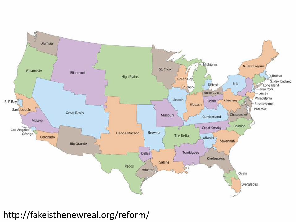
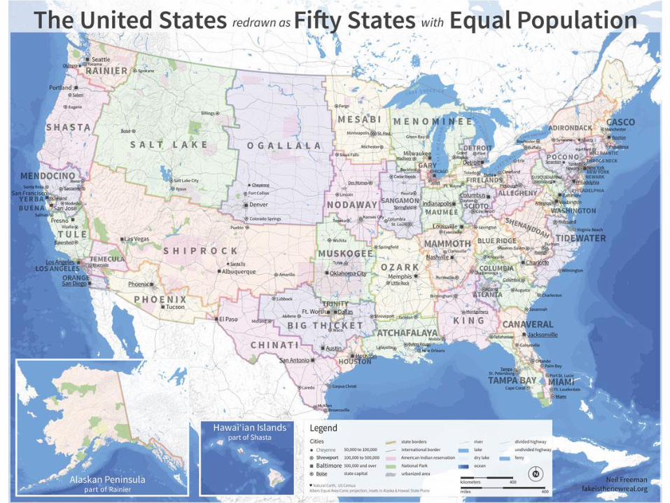
http://fakeisthenewreal.org/reform/

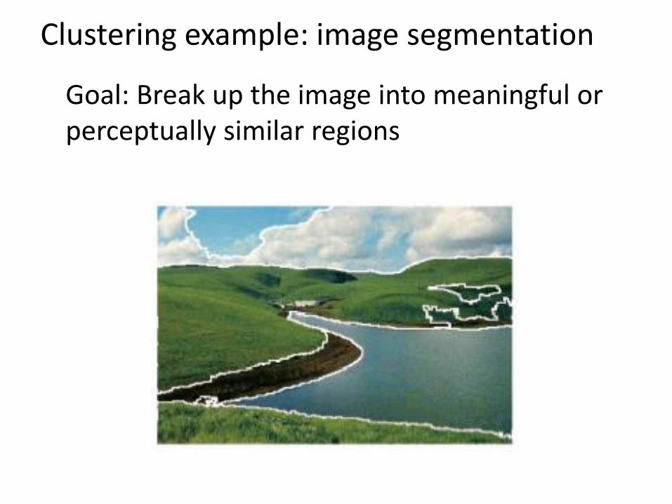
Clustering example: image segmentation

Goal: Break up the image into meaningful or perceptually similar regions

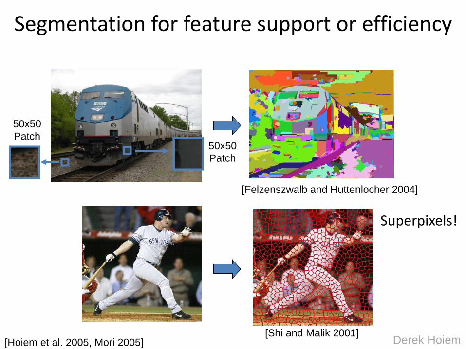
Segmentation for feature support or efficiency

[Felzenszwalb and Huttenlocher 2004]

[Hoiem et al. 2005, Mori 2005][Shi and Malik 2001]

Derek Hoiem

50x50

Patch

50x50

Patch

Superpixels!

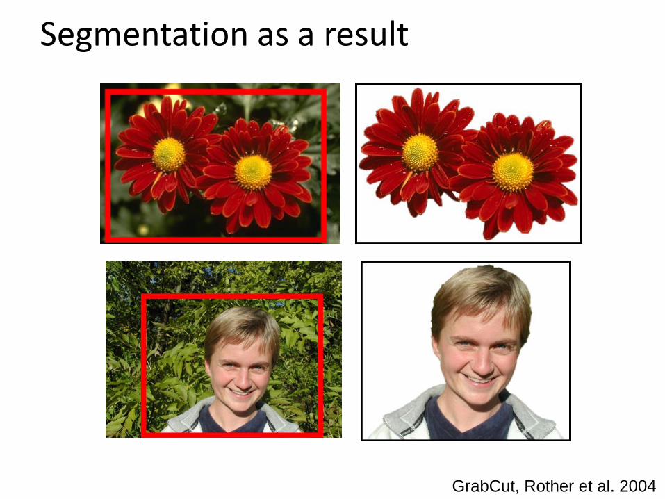
Segmentation as a result

GrabCut, Rother et al. 2004

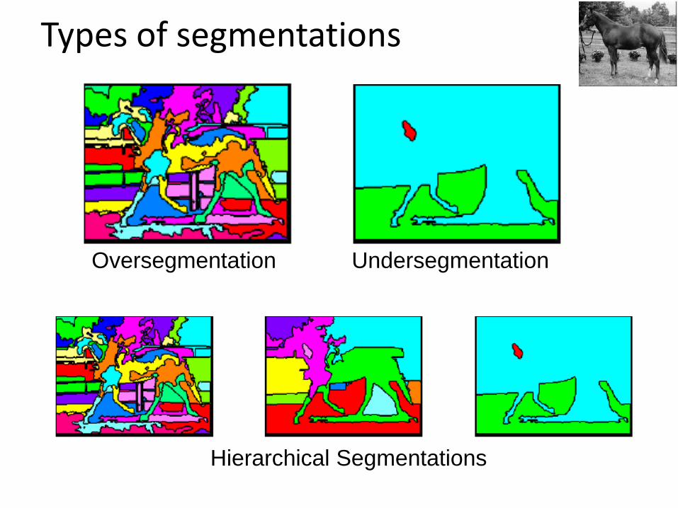
Types of segmentations

Oversegmentation Undersegmentation

Hierarchical Segmentations

Clustering

Group together similar ‘points’ and represent them with a single token.

Key Challenges:

1) What makes two points/images/patches similar?

2) How do we compute an overall grouping from pairwise similarities?

Derek Hoiem

Why do we cluster?

• Summarizing data– Look at large amounts of data– Patch-based compression or denoising– Represent a large continuous vector with the cluster number

• Counting– Histograms of texture, color, SIFT vectors

• Segmentation– Separate the image into different regions

• Prediction– Images in the same cluster may have the same labels

Derek Hoiem

How do we cluster?

• K-means– Iteratively re-assign points to the nearest cluster center

• Agglomerative clustering– Start with each point as its own cluster and iteratively

merge the closest clusters

• Mean-shift clustering– Estimate modes of pdf

• Spectral clustering– Split the nodes in a graph based on assigned links with

similarity weights

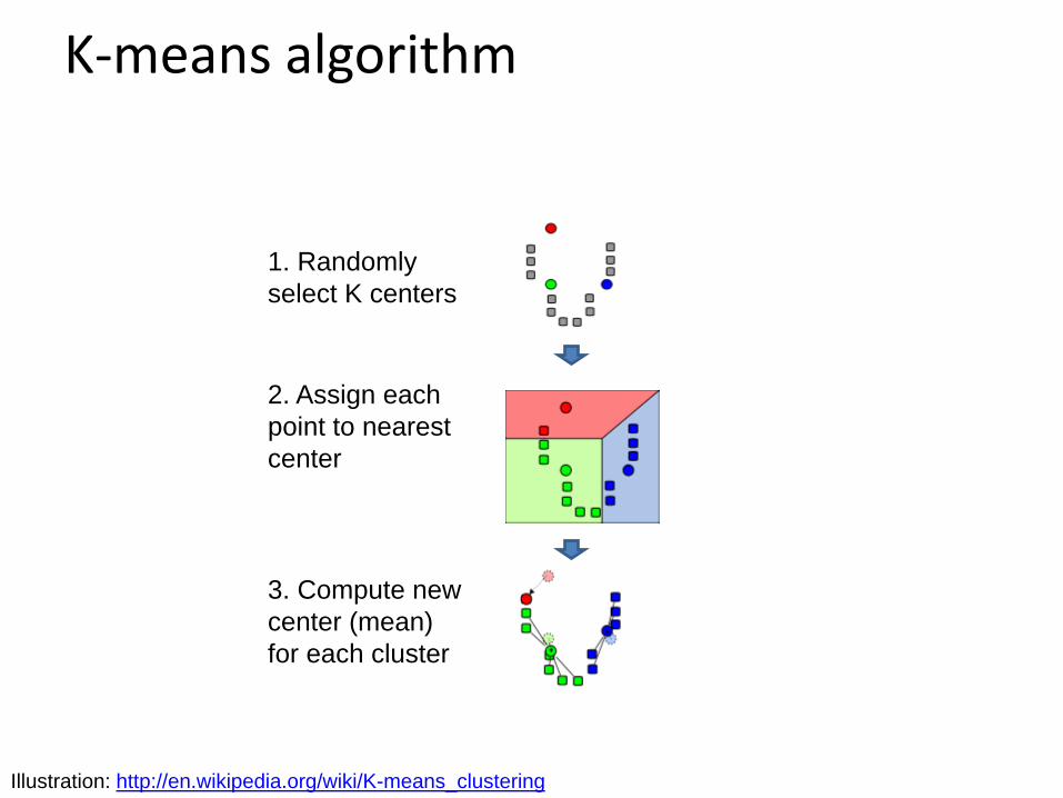
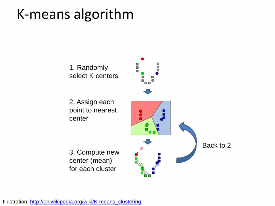
K-means algorithm

Illustration: http://en.wikipedia.org/wiki/K-means_clustering

1. Randomly

select K centers

2. Assign each

point to nearest

center

3. Compute new

center (mean)

for each cluster

K-means algorithm

Illustration: http://en.wikipedia.org/wiki/K-means_clustering

1. Randomly

select K centers

2. Assign each

point to nearest

center

3. Compute new

center (mean)

for each cluster

Back to 2

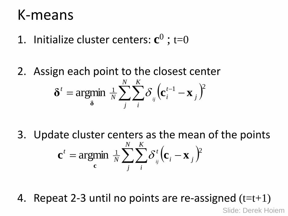
K-means

1. Initialize cluster centers: c0 ; t=0

2. Assign each point to the closest center

3. Update cluster centers as the mean of the points

4. Repeat 2-3 until no points are re-assigned (t=t+1)

N

j

K

i

j

t

iN

t

ij

211argmin xcδδ

N

j

K

i

ji

t

N

t

ij

21argmin xccc

Slide: Derek Hoiem

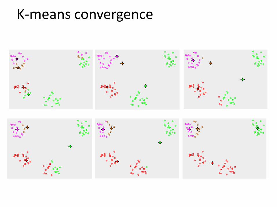
K-means convergence

Think-Pair-Share

• What is good about k-means?

• What is bad about k-means?

• Where could you apply k-means?

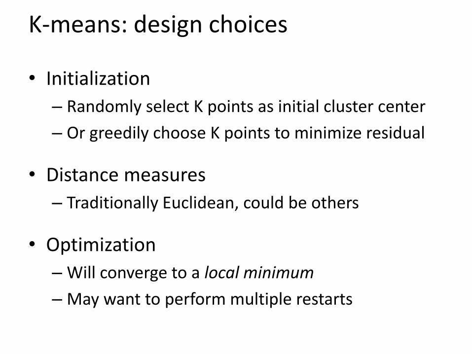
K-means: design choices

• Initialization

– Randomly select K points as initial cluster center

– Or greedily choose K points to minimize residual

• Distance measures

– Traditionally Euclidean, could be others

• Optimization

– Will converge to a local minimum

– May want to perform multiple restarts

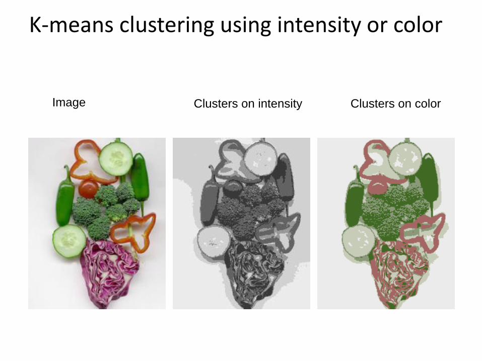
Image Clusters on intensity Clusters on color

K-means clustering using intensity or color

How to choose the number of clusters?

• Validation set

– Try different numbers of clusters and look at performance

• When building dictionaries (discussed later), more clusters typically work better.

Slide: Derek Hoiem

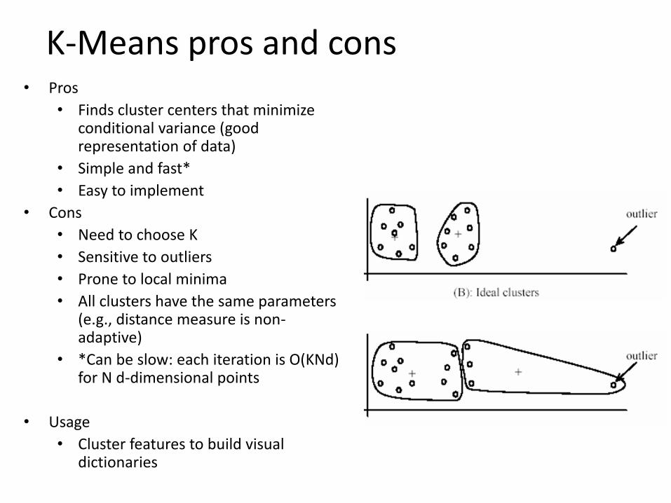
K-Means pros and cons• Pros

• Finds cluster centers that minimize conditional variance (good representation of data)

• Simple and fast*

• Easy to implement

• Cons

• Need to choose K

• Sensitive to outliers

• Prone to local minima

• All clusters have the same parameters (e.g., distance measure is non-adaptive)

• *Can be slow: each iteration is O(KNd) for N d-dimensional points

• Usage

• Cluster features to build visual dictionaries

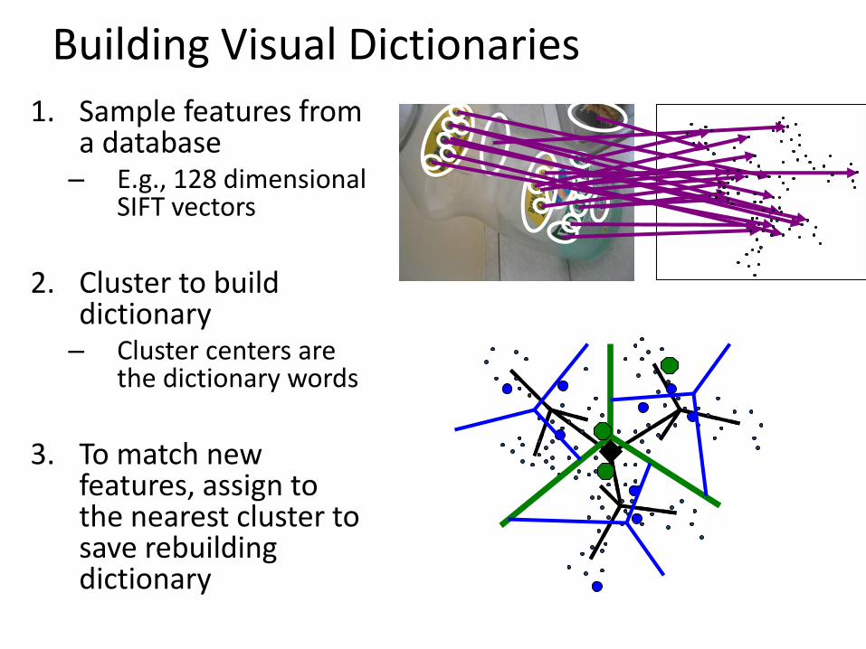
Building Visual Dictionaries

1. Sample features from a database

– E.g., 128 dimensional SIFT vectors

2. Cluster to build dictionary

– Cluster centers are the dictionary words

3. To match new features, assign to the nearest cluster to save rebuilding dictionary

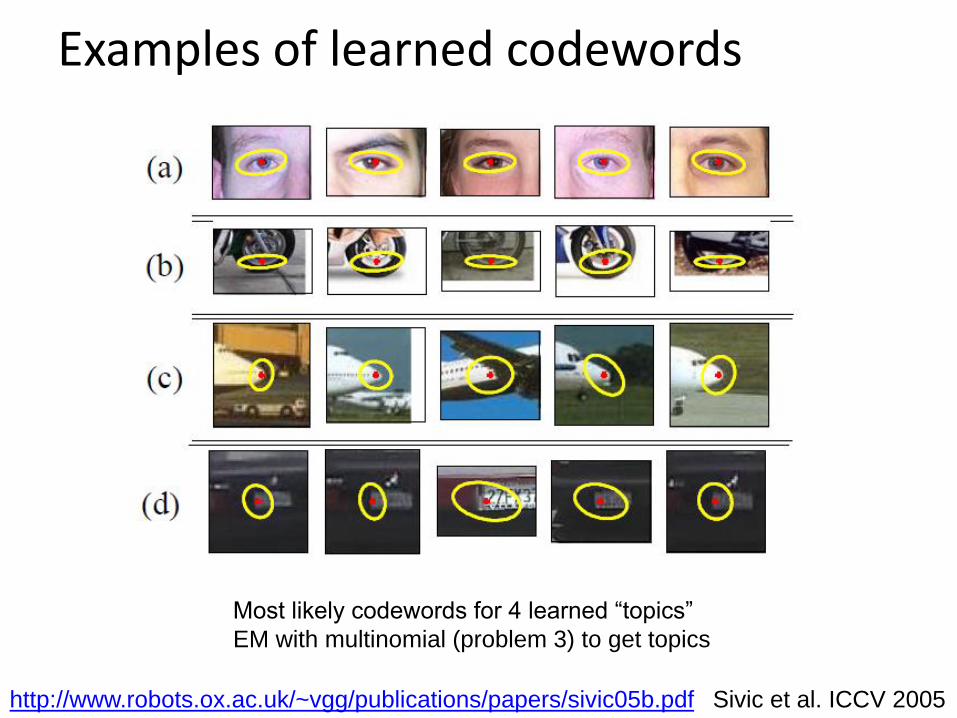
Examples of learned codewords

Sivic et al. ICCV 2005http://www.robots.ox.ac.uk/~vgg/publications/papers/sivic05b.pdf

Most likely codewords for 4 learned “topics”

EM with multinomial (problem 3) to get topics

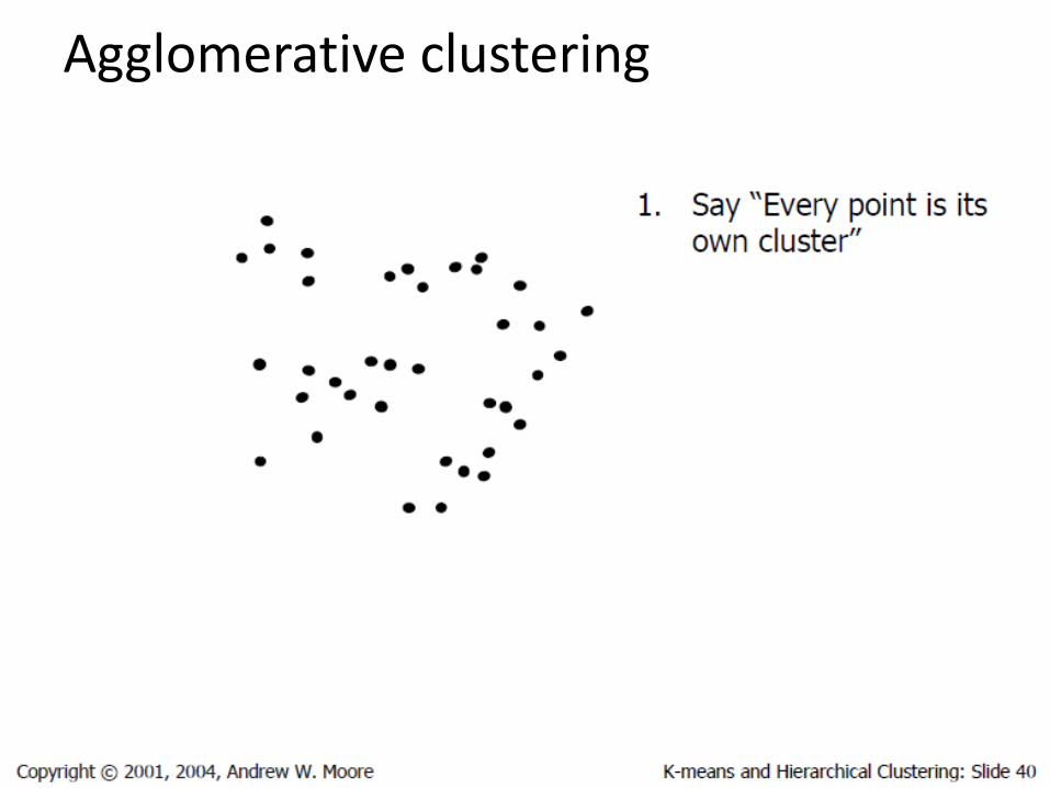
Agglomerative clustering

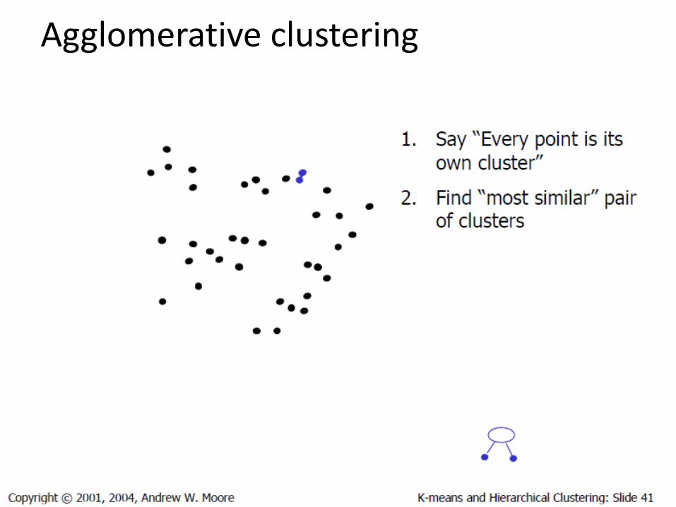
Agglomerative clustering

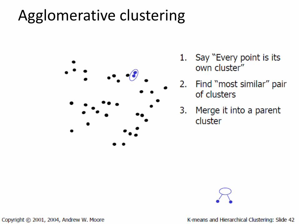
Agglomerative clustering

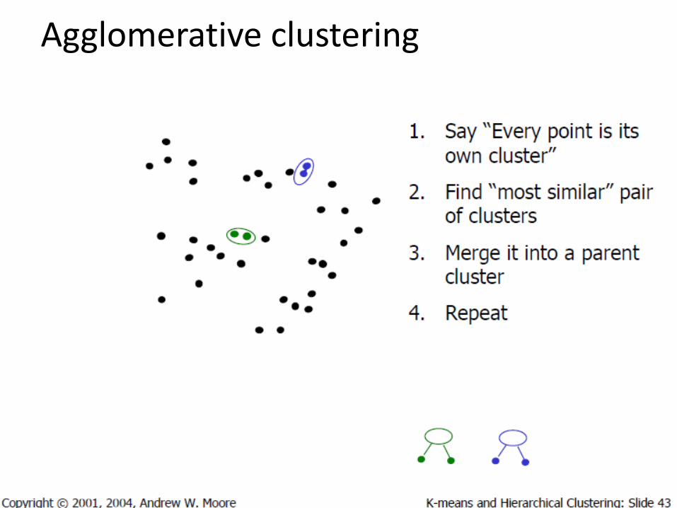
Agglomerative clustering

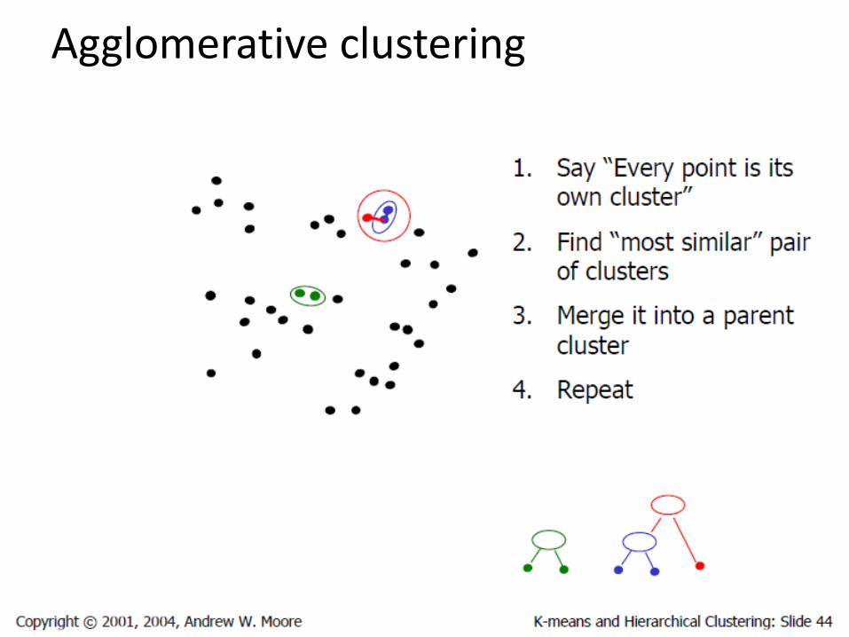
Agglomerative clustering

Agglomerative clustering

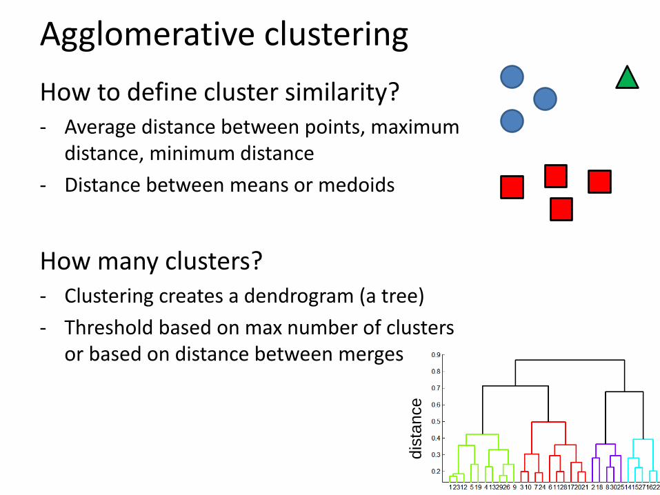
How to define cluster similarity?- Average distance between points, maximum

distance, minimum distance

- Distance between means or medoids

How many clusters?- Clustering creates a dendrogram (a tree)

- Threshold based on max number of clusters or based on distance between merges

dis

tance

Conclusions: Agglomerative Clustering

Good• Simple to implement, widespread application• Clusters have adaptive shapes• Provides a hierarchy of clusters

Bad• May have imbalanced clusters• Still have to choose number of clusters or

threshold• Need to use an “ultrametric” to get a meaningful

hierarchy

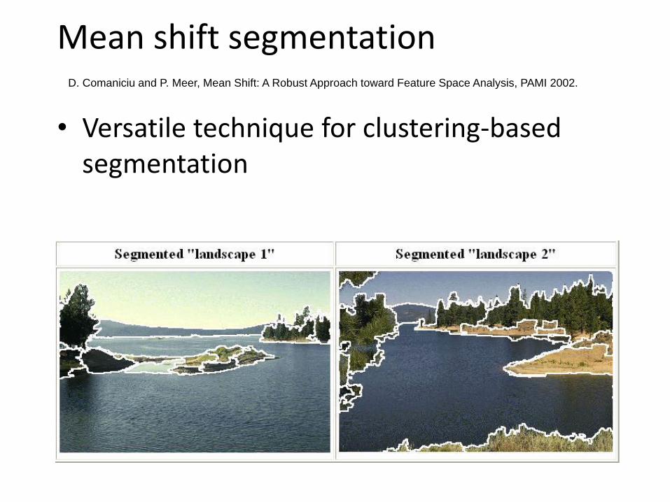
• Versatile technique for clustering-based segmentation

D. Comaniciu and P. Meer, Mean Shift: A Robust Approach toward Feature Space Analysis, PAMI 2002.

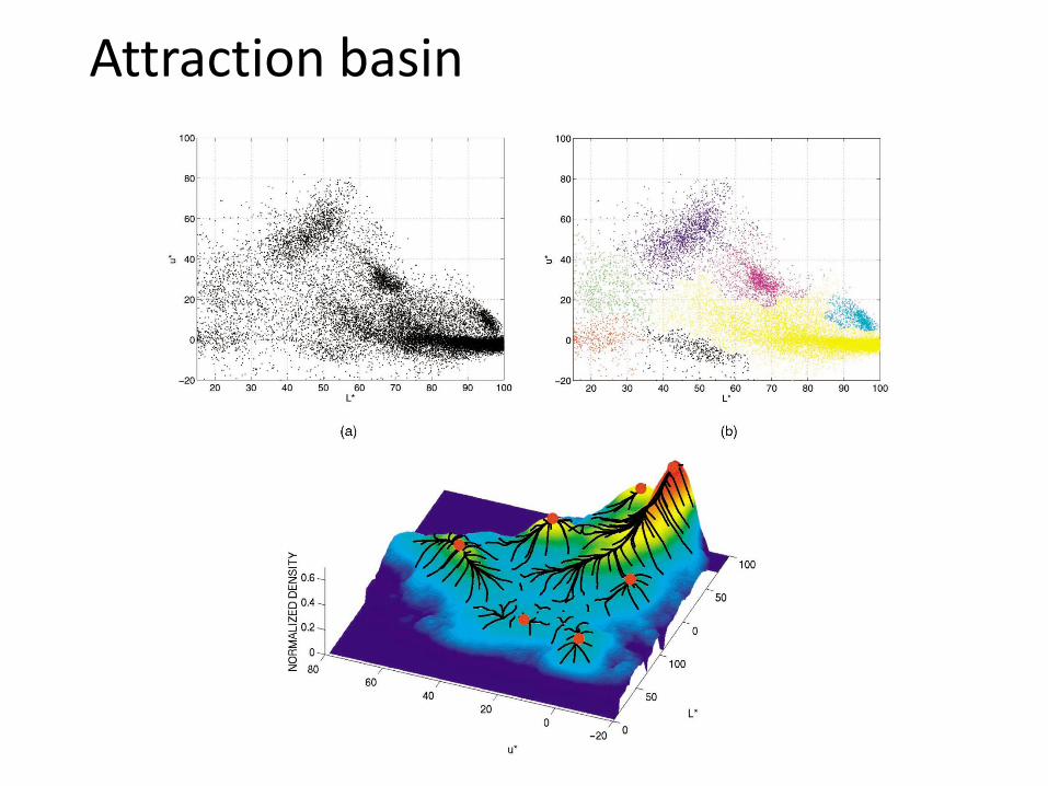
Mean shift segmentation

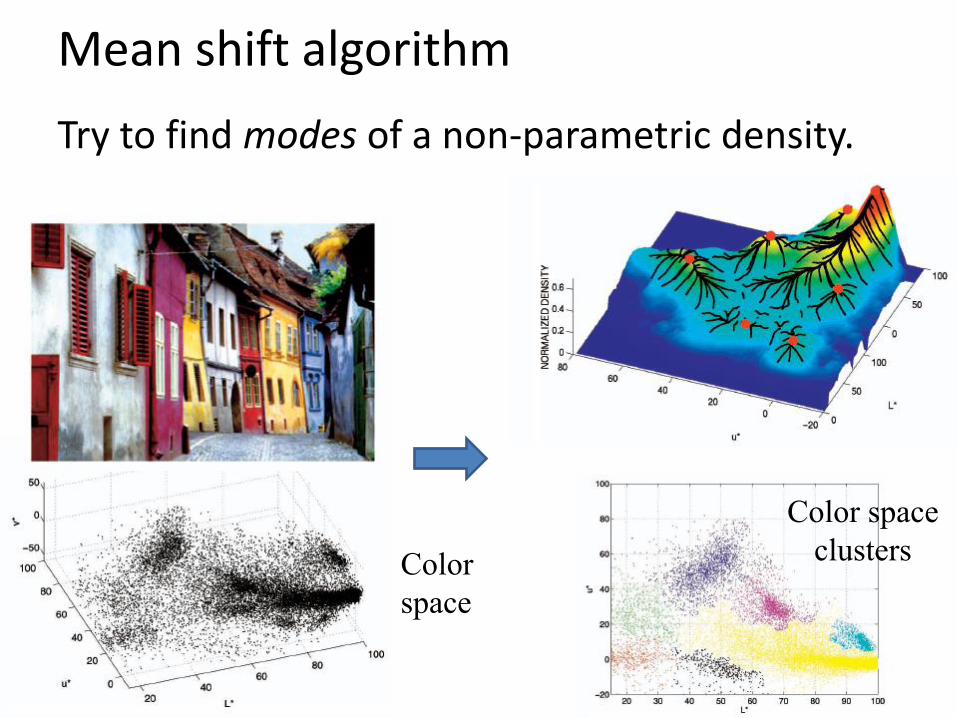
Mean shift algorithm

Try to find modes of a non-parametric density.

Color

space

Color space

clusters

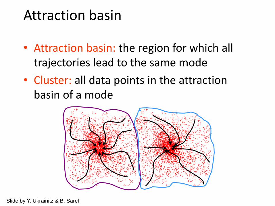
• Attraction basin: the region for which all trajectories lead to the same mode

• Cluster: all data points in the attraction basin of a mode

Slide by Y. Ukrainitz & B. Sarel

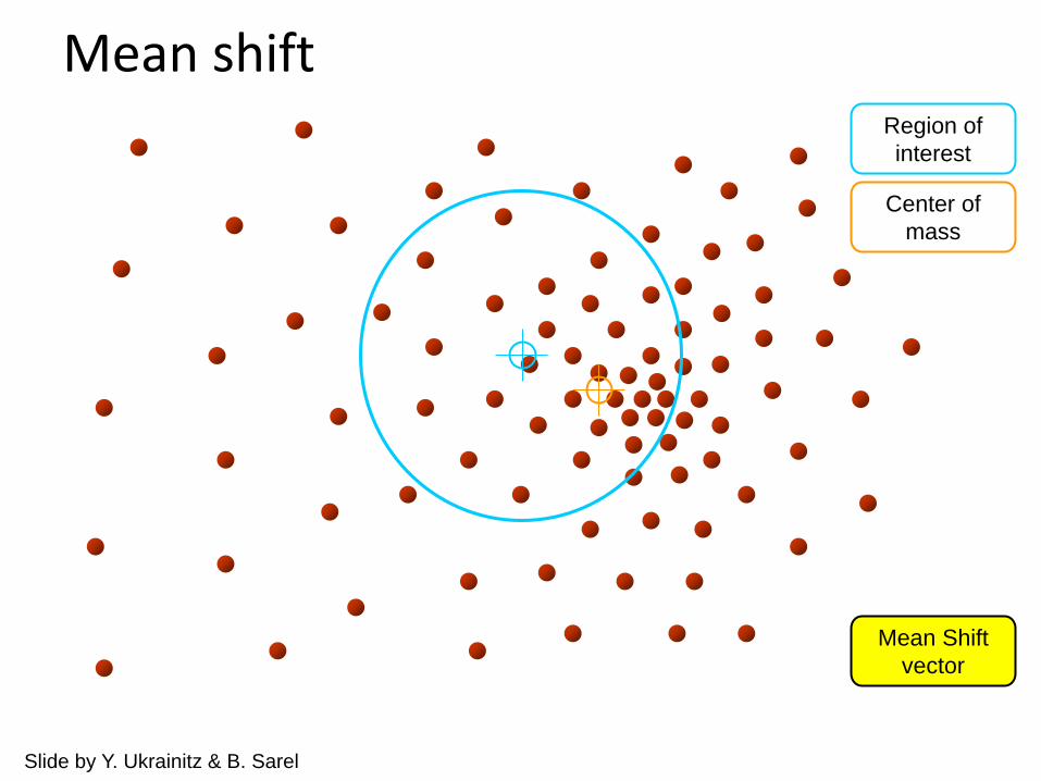
Attraction basin

Attraction basin

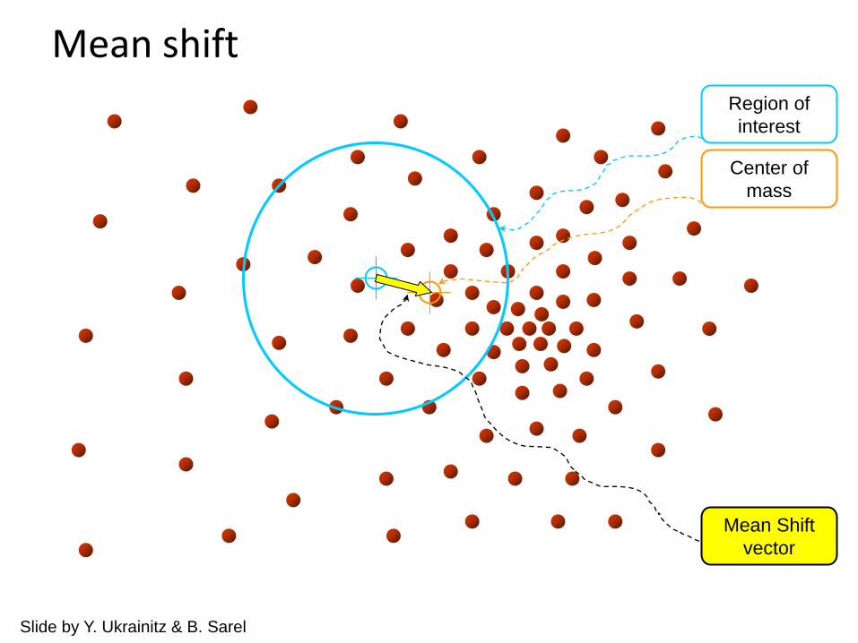
Region of

interest

Center of

mass

Mean Shift

vector

Slide by Y. Ukrainitz & B. Sarel

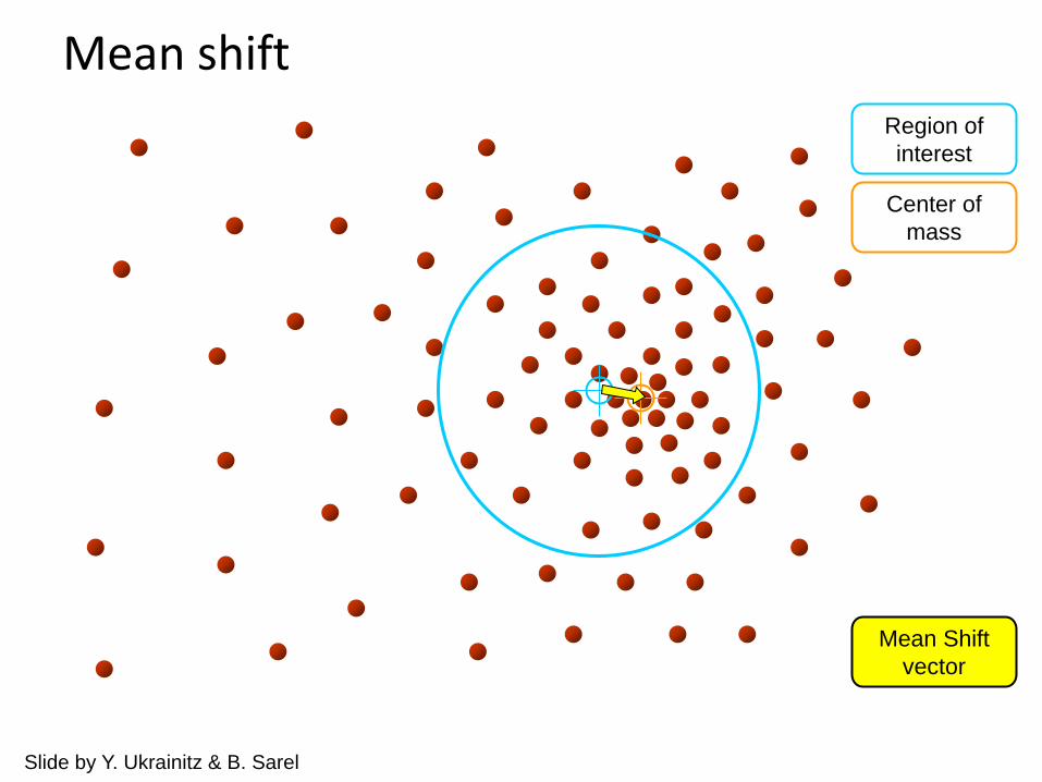
Mean shift

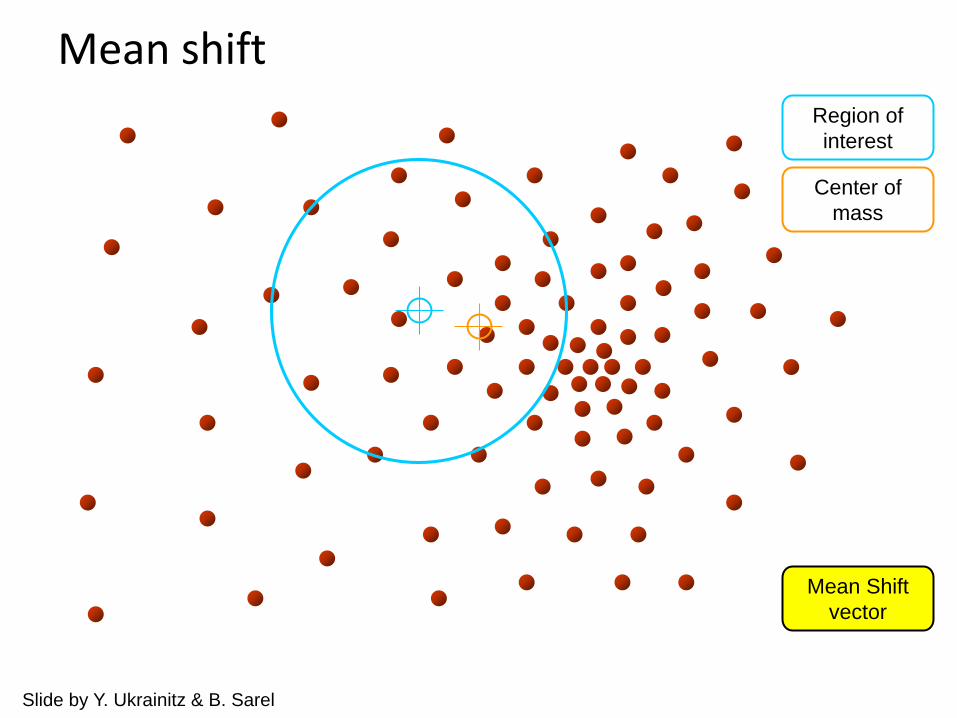
Region of

interest

Center of

mass

Mean Shift

vector

Slide by Y. Ukrainitz & B. Sarel

Mean shift

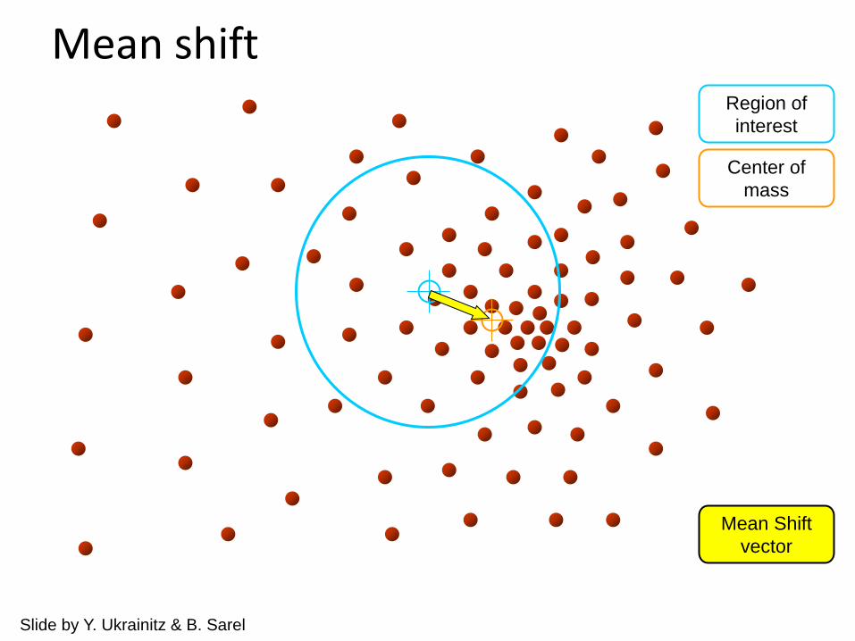
Region of

interest

Center of

mass

Mean Shift

vector

Slide by Y. Ukrainitz & B. Sarel

Mean shift

Region of

interest

Center of

mass

Mean Shift

vector

Mean shift

Slide by Y. Ukrainitz & B. Sarel

Region of

interest

Center of

mass

Mean Shift

vector

Slide by Y. Ukrainitz & B. Sarel

Mean shift

Region of

interest

Center of

mass

Mean Shift

vector

Slide by Y. Ukrainitz & B. Sarel

Mean shift

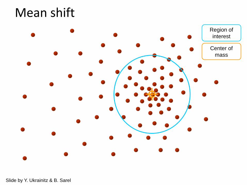
Region of

interest

Center of

mass

Slide by Y. Ukrainitz & B. Sarel

Mean shift

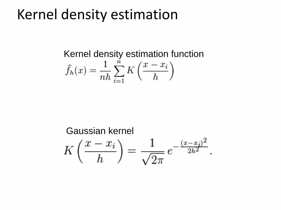
Kernel density estimation

Kernel density estimation function

Gaussian kernel

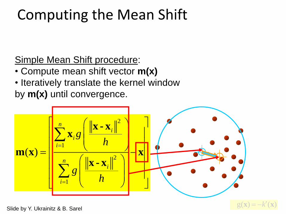
Simple Mean Shift procedure:

• Compute mean shift vector m(x)

• Iteratively translate the kernel window

by m(x) until convergence.

2

1

2

1

( )

ni

i

i

ni

i

gh

gh

x - xx

m x xx - x

g( ) ( )k x x

Computing the Mean Shift

Slide by Y. Ukrainitz & B. Sarel

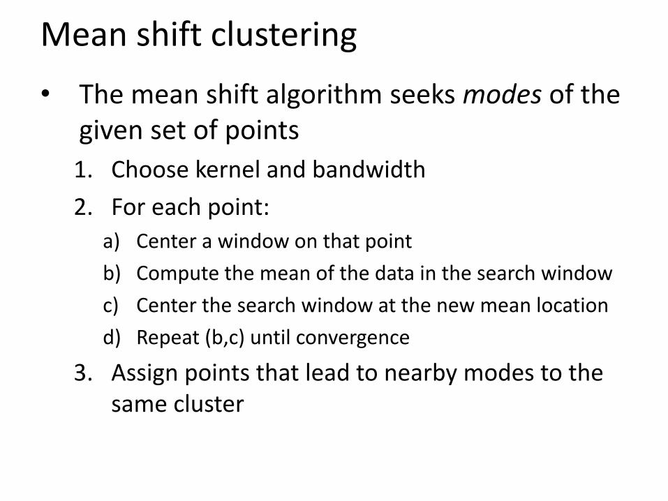
Mean shift clustering

• The mean shift algorithm seeks modes of the given set of points

1. Choose kernel and bandwidth

2. For each point:

a) Center a window on that point

b) Compute the mean of the data in the search window

c) Center the search window at the new mean location

d) Repeat (b,c) until convergence

3. Assign points that lead to nearby modes to the same cluster

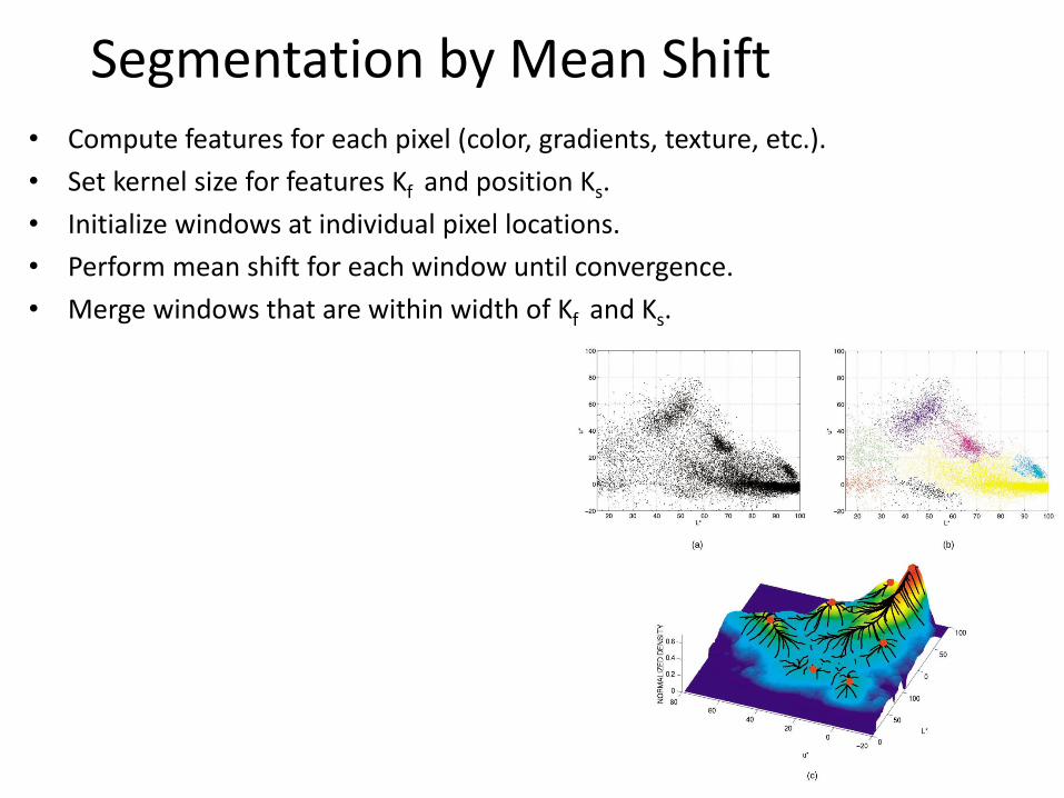
• Compute features for each pixel (color, gradients, texture, etc.).

• Set kernel size for features Kf and position Ks.

• Initialize windows at individual pixel locations.

• Perform mean shift for each window until convergence.

• Merge windows that are within width of Kf and Ks.

Segmentation by Mean Shift

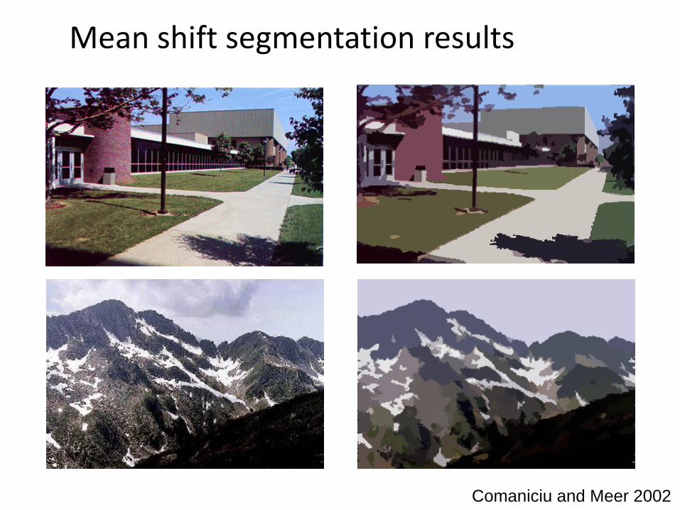
Mean shift segmentation results

Comaniciu and Meer 2002

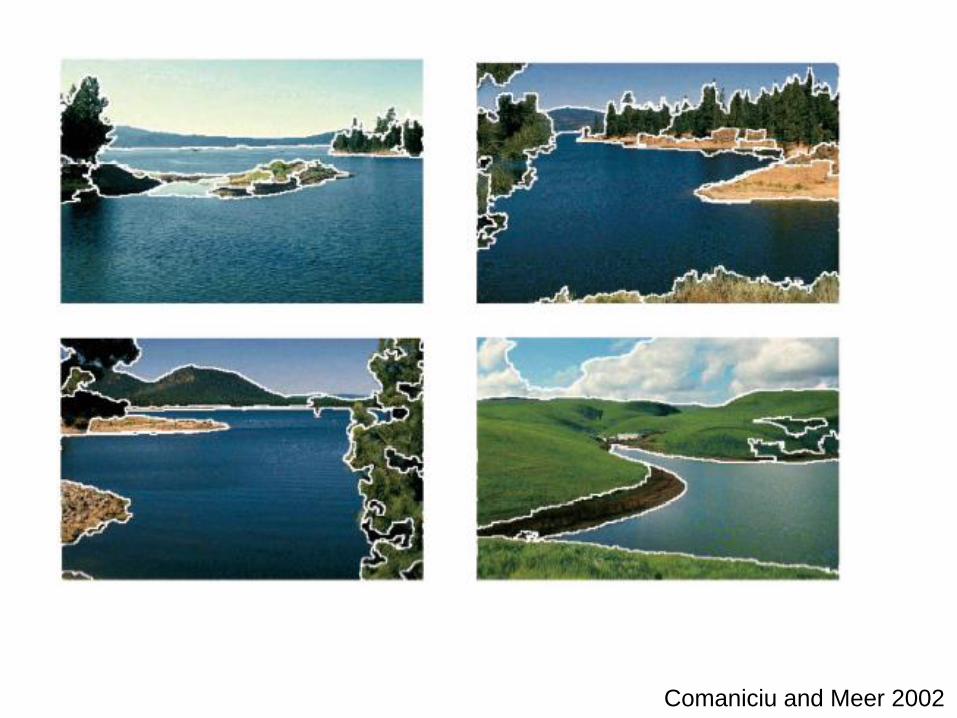
Comaniciu and Meer 2002

Mean shift pros and cons

• Pros

– Good general-practice segmentation

– Flexible in number and shape of regions

– Robust to outliers

• Cons

– Have to choose kernel size in advance

– Not suitable for high-dimensional features

• When to use it

– Oversegmentation

– Multiple segmentations

– Tracking, clustering, filtering applications

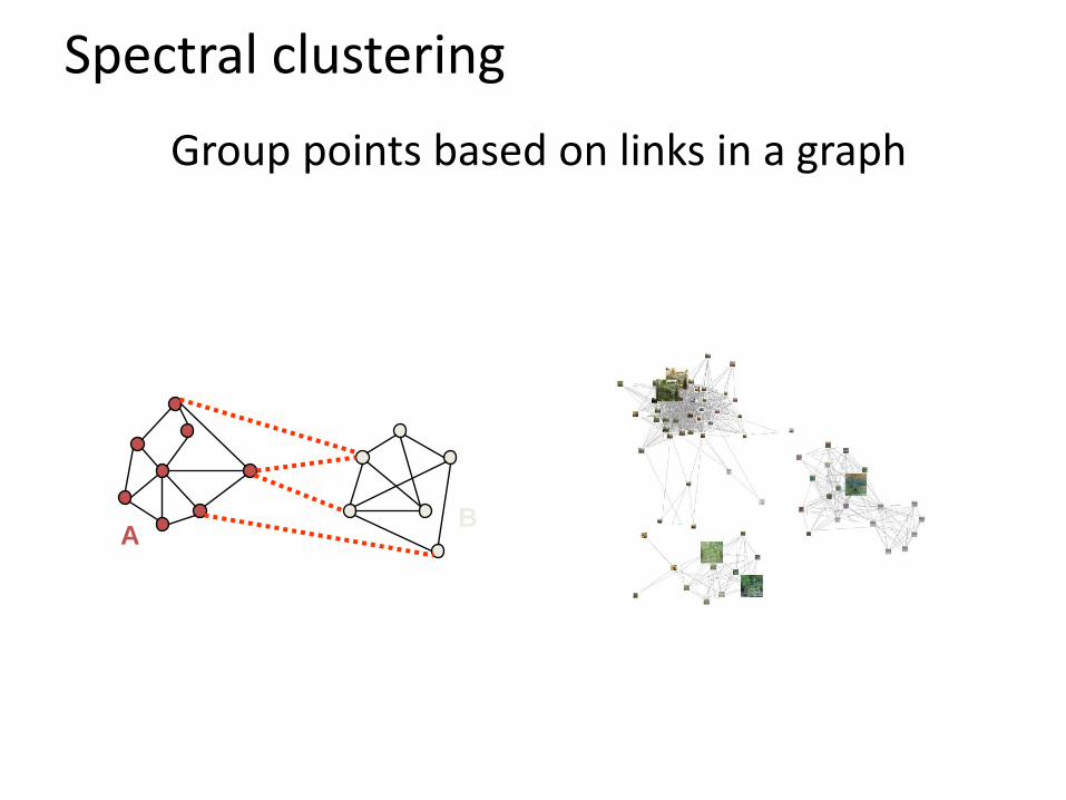
Spectral clustering

Group points based on links in a graph

AB

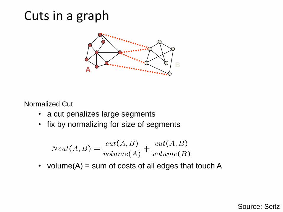
Cuts in a graph

AB

Normalized Cut

• a cut penalizes large segments

• fix by normalizing for size of segments

• volume(A) = sum of costs of all edges that touch A

Source: Seitz

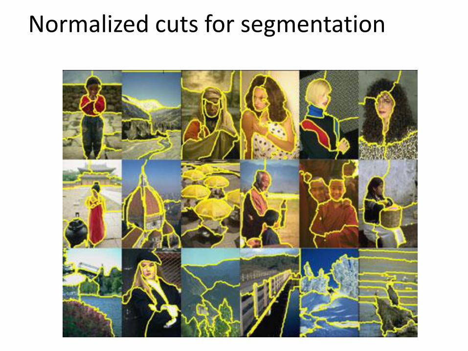
Normalized cuts for segmentation

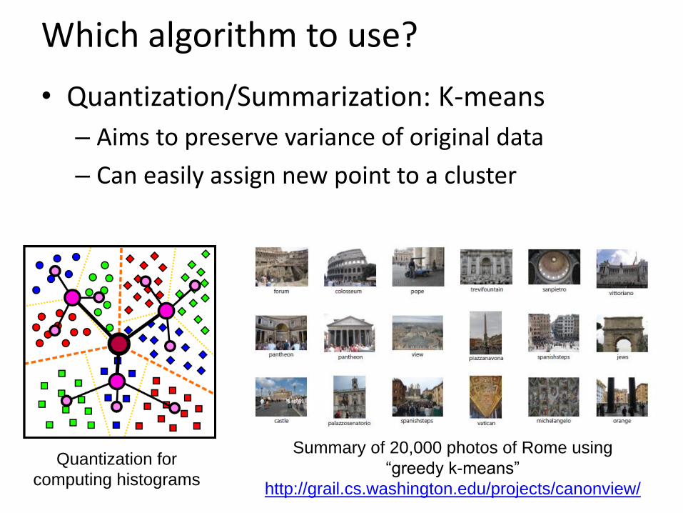
Which algorithm to use?

• Quantization/Summarization: K-means

– Aims to preserve variance of original data

– Can easily assign new point to a cluster

Quantization for

computing histograms

Summary of 20,000 photos of Rome using

“greedy k-means”

http://grail.cs.washington.edu/projects/canonview/

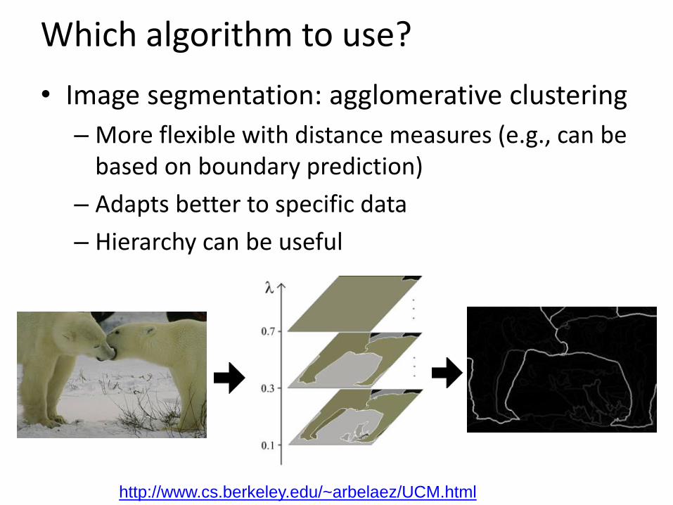
Which algorithm to use?

• Image segmentation: agglomerative clustering

– More flexible with distance measures (e.g., can be based on boundary prediction)

– Adapts better to specific data

– Hierarchy can be useful

http://www.cs.berkeley.edu/~arbelaez/UCM.html

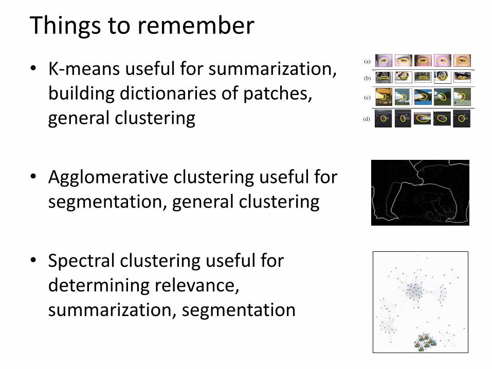
Things to remember

• K-means useful for summarization, building dictionaries of patches, general clustering

• Agglomerative clustering useful for segmentation, general clustering

• Spectral clustering useful for determining relevance, summarization, segmentation