1

Simple Analog Signal Chaotic Masking and Recovery

Christopher R. Comfort University of California, San Diego

Physics 173 Spring 2012

ccomfort@ucsd.edu

Abstract

As a major field of study, chaos is relatively new [1]. Much like how the invention of the telescope was needed to make pivotal advancements in early astronomy, the computer is the necessary tool of choice for chaosticians [1]. A novel and interesting application of chaos that has been introduced since Edward Lorenz first proposed “The Butterfly Effect” in 1972 to describe a system’s sensitive dependence on its initial conditions is signal masking or encryption. The goal of this experiment was to design a simple chaotic masking circuit using the eponymous Chua diode first in simulation using LT (Linear Technologies) SPICE (“spice”) and subsequently realizing the circuit physically with a comparative analysis of results.

I. Introduction

Before a signal is encrypted with chaotic weirdness, a reasonable question to ask is, “What is

chaos?” This is one of those terms that may have a different meaning depending on if you’re asking a

scientist, mathematician, or someone else. In the public sphere, chaos is skewed slightly negatively with

attributes such as randomness, disorder, and even anarchy. The mathematicians and physicists are still

trying to figure it out and definitions seem to vary depending on which elements of chaos are being

studied for a particular application. Most professionals agree that chaotic systems are very sensitive to

their initial conditions and all chaotic systems are nonlinear, but not all non-linear systems are chaotic

[1]. A safe and succinct definition is that chaos is a piece of jargon used to describe a type of

deterministic, nonlinear dynamical system that is very sensitive to initial conditions [1]. Sensitivity to

initial conditions simply means that two points starting very close together that share the same time

evolution equations will diverge wildly soon after T0. This behavior normally doesn’t happen in linear

systems (or every nonlinear one). If two points in a linear system start very close together and share

2

common dynamical equations, their evolution through space-time will be very similar. This immediate

and dramatic divergence after T0 is a hallmark feature of chaos.

For the sake of brevity this paper will focus more on the circuit itself and not as a survey into the

specificities of chaotic dynamics; however, certain pertinent aspects of chaos theory will be brought up

as they are needed throughout the analysis.

II. Basic Chaotic Signal Masking

In its simplest form a chaotic masking circuit needs an input signal, a master chaos generator,

some sort of summing amplifier, a slave chaos generator, and a difference amplifier (See Fig. 1).

The master chaos generator produces a voltage that when viewed as a 1-D trace on an oscilloscope

looks like noise. When added to the original message signal the output should make the message

unrecognizable. To recover the signal, an exact copy of the master chaos signal needs to be available or

the original signal will look noisy. Synchronization of the master generator with a slave ideally made of

matched components causes their voltage dynamics to become identical which makes it possible to

replicate the unique chaotic masking waveform in real time that would otherwise be impossible to

achieve. By subtracting the slave signal with the master + original, theoretically an exact copy of the

Fig. 1: Block diagram of the basic components of an analog chaotic signal masking circuit.

3

original will be recovered. The ability for chaotic circuits to synchronize is why they’re of interest to

those working in encryption and other types of secured communication [6].

III. The Chua Circuit as a Chaos Generator

In the early 1980’s Leon Chua of the University of California, Berkeley, was the first to invent a

physical circuit that could accurately and repetitively exhibit chaotic dynamics with very simple, off the

shelf components. Its simplicity and reliability make it the perfect chaos generator for signal masking

[6].

At its core, the Chua circuit contains four passive linear components (two capacitors, one resistor, and

one inductor) and one active, nonlinear one: the Chua diode (see Fig. 2). Chua had proved that any

circuit containing solely passive components can never present chaotic dynamics [3]. Note that there is

no outside voltage source driving the circuit—all voltages across components, initial conditions for the

system, and the chaotic dynamics are stemming from thermal noise or properties of the op-amps within

the nonlinear resistor. For this experiment, all voltages to power active circuit components were

coming from a single regulated bench top DC power supply at 9.0 V.

Fig. 2: The Chua Circuit. Key traces are off “Vc1”, “Vc2”, and “IL1.” The boxed region can be thought of as a single component, the Chua diode or non-linear resistor.

4

When taking the nonlinear resistor portion of the circuit as a single component, deriving the

equations of state for the entire system becomes a rather simple exercise in Kirchhoff’s laws and the

mathematical relationships between voltage, current, and inductance:

𝐶1𝑑𝑉𝑐1

𝑑𝑡= 1

𝑅9(𝑉𝑐2 − 𝑉𝑐1) − 𝑔(𝑉𝑐1)

𝐶2𝑑𝑉𝑐2

𝑑𝑡=

1𝑅9

(𝑉𝑐1 − 𝑉𝑐2) + 𝐼𝐿1

𝐿 𝑑𝐼𝐿1𝑑𝑡

= −𝑉𝑐2,

(1)

where the function 𝑔(… ) is defined by:

𝑔(𝑉𝑅) = 𝑚0𝑉𝑅 +12

(𝑚1 − 𝑚0)��𝑉𝑅 + 𝐵𝑝� − �𝑉𝑅 − 𝐵𝑝�� (2)

and 𝑉𝑅 is the voltage across the Chua diode as a whole.

Ironically, this is a piece-wise linear function that describes the behavior of the nonlinear resistor

component of Chua’s circuit [3]. The nonlinear resistor acts as a negative impedance converter, meaning

that current is forced to flow from a lower voltage to a higher voltage instead of vice versa. The

attractors of the chaotic dynamics within the system are highly dependent on these negative regions in

the I-V (current-voltage) spectrum of the nonlinear resistor. Since resistance is related to current and

voltage via Ohm’s law it is implied that this negative resistance is proportional to negative currents and

voltages (quadrant’s II and IV on an I-V graph). But since there can’t be negative power: 𝑃 = 𝑉𝐼, all

physically buildable nonlinear resistors must eventually become passive for large V and I (See below) [3].

(A) (B)

Fig. 3: (A) shows the slopes and break points of the nonlinear resistor occupying quadrants II and IV. (B) shows the I-V curve for the nonlinear resistor graphed separately from the rest of Chua’s circuit in spice. It’s being driven with a triangle wave at 30 Hz with a small current sensing resistor from the drives negative terminal going to ground.

5

Notice in Fig. 3(B) that after saturation, the I-V curve returns to the passive positive regions in quadrants

I and III. This is out of range to exhibit chaos. Normal diodes generally have the same shaped curve only

occupying quadrants I and III (essentially, an inverted form of Fig. 3(B).)

In the above paragraph I mentioned “the attractors of the chaotic dynamics within the

system...” In nonlinear science an attractor is the point or the set of points in phase space where an

orbit will eventually tend towards throughout the time evolution of the system [2]. Attractors can be

simple, as in the damped harmonic oscillator, which has one as a single point at (0, 0) in (ω, θ) phase

space or quite complicated as they are in most chaotic systems. The Chua circuit has multiple attractors,

but its calling card is the so-called “double scroll strange attractor.” Why it’s called “strange” will be

touched on later.

(A)

(B)

(C)

Fig. 4 (from spice simulation): (B) and (C) shows the voltage traces Vc2 and Vc1 respectively from Chua’s circuit as a function of time. Notice that this can easily be construed for noise. But when graphed in phase space (A),Vc2 vs. Vc1 the beautiful “double scroll” attractor presents itself and it’s clear that this system is more than just noise.

6

IV. The Chaotic Masking Circuit (Simulation)

Now that some of the dynamics of Chua’s circuit has been introduced, its use as a chaos

generator in a simple chaotic masking circuit can be better appreciated.

The goal of this experiment was to design the simplest circuit possible that could exhibit chaotic

masking. The only components here that differ from those of Fig. 1 are the inverting amplifier at

“Vout2” and a buffering amplifier in the synch chain of the two chaos generators. The addition of the

inverter was arbitrary and obvious; however, the buffer proved to be essential while testing the circuit

with spice simulations (to be explained later). Chaotic dynamics can be extremely fickle and very

sensitive to subtle nuances in changes of voltages, currents, resistance, and who knows what other kinds

of variables. In isolation the Chua circuit may work perfect, but once it’s connected to other circuit

components all it takes is a little back feed or other miniscule change in the system and the chaos will

die and give way to periodicity.

Fig. 5: The schematic for a simple chaotic masking circuit. The input signal is a simple sine wave and the two chaos generators are symbolized by the boxes with the waveforms in them. The master generator is furthest left.

7

(A)

(B)

(C)

(D)

(E)

Fig. 6: Results from spice after a 1000 ms simulation. A snapshot of approximately 140 ms is shown with (E) being the original sine wave signal. (D) and (C) are the master and slave chaos generators respectively. Notice the synchronization of the complex waveforms. (B) is the masked signal, original + master. (A) is the recovered signal, masked – slave.

8

Fig. 6 shows a successful simulation of the chaotic masking circuit. The input sine wave (𝑉1) had a

frequency of 100 Hz with an amplitude of 500 mV (1 Vpp). Resistor values for the summing and

difference amplifiers were chosen to limit gain, but R2 and R5 had very high values to limit back feed

current into the chaos generators which was found to destroy the chaos if on the order of ~5.5 μA.

For the non-inverting summing amplifier with an input voltage of 1 Vpp and the master chaos

generator (𝑉𝑐ℎ𝑎𝑜𝑠1) with an input voltage of ~3.2 Vpp:

𝑉𝑜𝑢𝑡1[𝑉𝑖𝑛2] = �𝑉1𝑅2

𝑅1 + 𝑅2+ 𝑉𝑐ℎ𝑎𝑜𝑠1

𝑅1

𝑅1 + 𝑅2� �1 +

𝑅3

𝑅8� (3)

With resistor values of R1 = 20 kΩ, R2 = 150 kΩ, R8 = 100 kΩ, and R3 = 10 kΩ, 𝑉𝑜𝑢𝑡1[𝑉𝑖𝑛2] = 1.387 Vpp. This

was consistent with the experimental value found in Fig. 6(B).

For the difference amplifier:

𝑉𝑜𝑢𝑡 = �𝑅4 + 𝑅7

𝑅5 + 𝑅6�

𝑅6

𝑅4𝑉𝑐ℎ𝑎𝑜𝑠2 −

𝑅7

𝑅 4𝑉𝑜𝑢𝑡1[𝑉𝑖𝑛2]

(4)

𝑉𝑐ℎ𝑎𝑜𝑠2 had a value of 200 mVpp. For R4 = R6 = R7 = 10 Ω and R5 = 150 kΩ, 𝑉𝑜𝑢𝑡 had a value of 1.0 Vpp as

shown in Fig. 6(A) and was exactly as expected. Keeping R10 and R11 the same for the inverter maintained

a gain of 1 as to not affect the voltage coming out of the difference amplifier so the output voltage of

the circuit was exactly as original sine wave message signal.

The simulation did present a few quirks, however. During the course of multiple simulations, the

chaos generators would un-synch briefly for about 1-3 ms then re-align. This occurred only when the

buffer was included in the synch chain. Without the buffer, the simulation would not go past 500 ms

without losing chaos and reverting to periodicity. I speculate that current back feed would creep from

the slave generator into the master annihilating chaos. With the buffer in place, when the difference in

current registered a voltage change, the buffer immediately (almost) equated input with output,

keeping the circuit in the chaotic regime. I speculate these little errors in un-synching were the result of

the current back feed trying to kill the chaos, but being halted by the buffer in 1-3 ms. These errors

manifested themselves as little blips in the troughs and/or crests in the recovered waveform. Even with

the errors, I think the buffer was necessary to maintain chaos in the circuit. It should be noted that

adding the buffer in the synch chain really slowed down the computation time. It took about 10 min per

100 ms of the simulation.

There were also interesting little delays in the chaos generators at T0. It took about 8 ms for the

generators to kick in which was very odd. Thinking delaying the input sine wave would solve the issue;

this was attempted to no avail. The delay of the chaos generators were simply shifted alongside the

9

delay of input sine wave at exactly 8 ms. No satisfactory hypotheses were explored to rectify the issue

and it was forgotten when the actual circuit was not found to have the same problem.

(E)

(D)

(C)

(B)

(A)

Fig. 7: Un-synching and re-aligning in the simulation with the added buffer in the synch chain. (E) is the original signal. (D) and (C) are the master and slave generators respectively as in Fig. 6. Notice at about 57 ms the two generators become un-synched then quickly re-align. Masking (B) is unaffected, but the recovered signal (A) has a distinctive “hump” in the trough of the wave.

10

V. The Chaotic Masking Circuit (Actual)

The actual circuit was constructed on a solderless breadboard exactly as it was designed in spice

with the same resistor values. Spice uses ideal components whose behaviors may deviate from those in

the real world. The op-amps used in the simulation were the LT1007’s—low noise, high speed. The

LM358AN dual op-amps were chosen as replacements because they exhibit similar qualities and do well

in the audio frequency range. First, one Chua circuit was built with successful occurrences of chaos

proven by viewing traces on the oscilloscope. Then the second one was built and also tested. The rest of

Fig. 8: Delay in the chaos generators. Notice the masking [V(n003)] and [V(vout1[vin2])] doesn’t start until the chaos generators [V(chaos1)] and [V(chaos2)] kick in at about 8 ms after T0.

11

the circuit was added and data was acquired from nine traces and analyzed in Matlab: 3 from each state

variable of the chaos generators (Vc1, Vc2, and IL1), the original signal, the masked signal, and finally the

recovered signal.

8300 8350 8400 8450 8500 8550-3

-2

-1

0

1

2

3

Samples/Second

Vol

tage

Vc1

1.035 1.04 1.045 1.05 1.055 1.06

x 104

-0.8

-0.6

-0.4

-0.2

0

0.2

0.4

0.6

Samples/Second

Vol

tage

Vc2

Fig. 9: Vc1 from the master chaos generator graphed against samples/second (time). Note the similarity in waveform with Fig. 4(C).

Fig. 10: Vc2 from the master generator graphed against time. Note the similarity in waveform with Fig. 4(B).

12

-3 -2 -1 0 1 2 3-0.8

-0.6

-0.4

-0.2

0

0.2

0.4

0.6

Vc1 Chaos Generator 1

Vc2

Cha

os G

ener

ator

1Vc1 vs. Vc2 for Chaos Generator 1, O-scope Waveform

-3 -2 -1 0 1 2 3-0.8

-0.6

-0.4

-0.2

0

0.2

0.4

0.6

Vc1 Generator 1

Vc2

Gen

erat

or 2

-0.2 -0.1 0 0.1 0.2 0.3 0.4 0.5-0.12

-0.1

-0.08

-0.06

-0.04

-0.02

0

0.02

0.04

Vc1 Generator 1

Vc2

Gen

erat

or 2

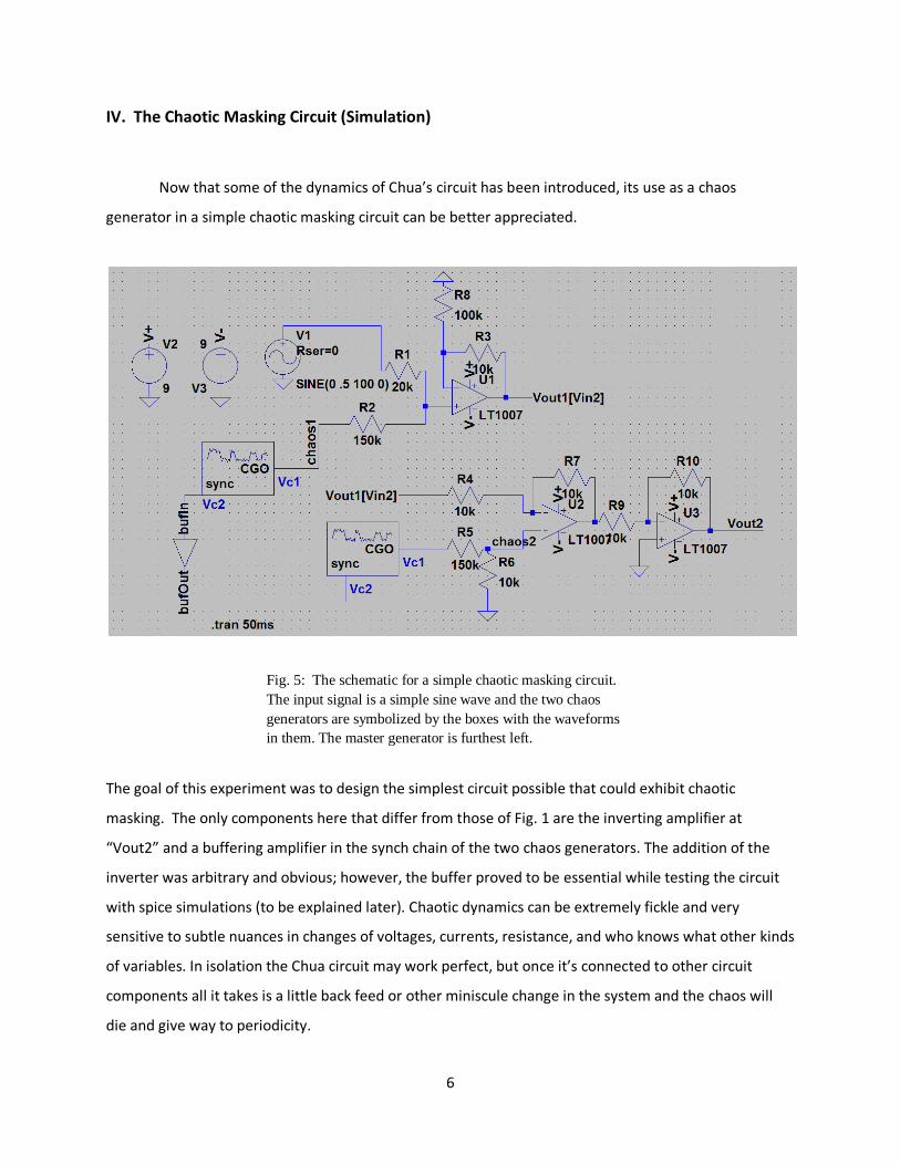
Fig. 11: Double scroll attractor taking a trace from the master generator to one on the slave to show that chaos is maintained through the synchronization.

(A) (B)

Fig. 12: Double scroll attractor as graphed in Matlab, again taking traces from the master Vc1 to the slave Vc2. Data was taken at 20,000 samples/second so the graph (A) looks washed out. (B) shows a 10x view taken from near the center of the attractor to see the paths more clearly.

13

Figs. 11 and 12 show two dimensional projections of the double scroll strange attractor when in

actuality, chaos is at least a three dimensional phenomena. Part of the complexity of chaotic dynamics

is that the orbits in phase space never repeat nor cross each other [1,2]. A system must have at least

three dimensions to achieve this.

The Z axis on Fig. 13 shows Vc2 – VL1. This was taken as a proxy for the current going through

the inductor. From Ohm’s law V ∝ I and it has been previously shown that this relation holds true for

Vc2 –VL1 in Chua’s circuit [2]. Recall from (1) that current through the inductor is a state equation of the

system along with the voltages across the two capacitors. All other time variables in the circuit end up

being dependent on those three equations [1]. Graphing the three state variables in phase space gives

the most accurate visualization of the chaotic dynamics in Chua’s circuit and voltages are easier to

handle with oscilloscopes and signal processing.

-4-2

02

4

-1-0.5

00.5

1-3

-2

-1

0

1

2

3

Vc1 Generator 1Vc2 Generator 2

Vc2

Gen

1 -

VL1

(pro

porti

onal

to I L1)

Fig. 13: 3-D representation of the double scroll attractor. Again, at 20,000 samples/second the data seems to wash out the graph, but zooming in would show a similar pattern as seen in Fig. 12(B).

14

-3 -2 -1 0 1 2 3-3

-2

-1

0

1

2

3

V (Chaos2)

V (C

haos

1)

y = 0.96*x + 0.016

data 1

linear

Fig. 14 (above) from the actual circuit shows Vc1 in the master generator to Vc1 in the slave generator. If they were perfectly synched this relationship would tend towards a straight line with a slope of 1. Fig. 15 (below) shows the same variables graphed against each other in spice with slightly different scaling.

15

A simple way to test the synchronization of two chaos generators is to graph one of the state

variables that weren’t used as the synch hub to its exact counterpart in the other circuit. For example, in

this particular setting, the chaos generators were combined at Vc2 on both circuits so to test whether

they were displaying exact dynamics one simply needs to graph Vc1 on the master generator to Vc1 on

the slave generator. This graph should look like a straight line (See Figs. 15 and 16). When testing the

two chaos generators in spice before the rest of the circuit was hooked up to them, their

synchronization was a perfect line—not surprising in a simulation environment with ideal components.

Interestingly, once the rest of the circuit was included and everything was running, even spice deviated

from a perfect line (See Fig. 16). The actual circuit didn’t fare too bad considering none of the cross

constituents of the master and slave generators were really “matched”—meaning values were taken

with a multi-meter of each component and only ones which deviated from a tiny pre-determined margin

of error were used. Care was taken to use the exact make and models of individual parts in the Chua

circuits.

The signal masking was not as prominent in the actual circuit as it was in the spice facsimiles

(See Fig. 16 above). It was noticed during the circuit simulations that there was a strong correlation

between the amplitude of the input sine wave signal, the value of R1, and the quality of the masking

signal. As noted above, the input sine wave oscillated between 500 mV and -500 mV at 100 Hz and the

value of R1 was optimized for this input voltage. In the actual circuit; however, the function generator

2380 2390 2400 2410 2420 2430 2440 2450-2.5

-2

-1.5

-1

-0.5

0

0.5

1

1.5

2

2.5

time (arbitrary)

Vol

tage

Original signalMasked signalRecovered signal

Fig. 16: Graph of the original, masked, and recovered signals against an arbitrary time scale and adjusted voltage scale.

16

could not sustain an amplitude that low so it was adjusted to about 1.5 Vpp, oscillating from roughly 750

mV to -750 mV. The value of R1 was not changed to reflect the new input voltage which consequently

could have compromised the quality of signal masking.

VI. Fractal Dimensions and Lyapunov Exponents

The signal processing power of Matlab and its vast network of m.file sharing makes it a much

less of an arduous task to examine some very interesting higher level mathematical properties of chaos,

notably, the geometry of chaotic attractors and quantifying their dimensionality. Two such quantitative

characteristics will be discussed – fractal dimension, and Lyapunov exponents.

Benoit Mandelbrot coined the term fractal in 1982 to describe the non-integer dimensional

space that certain geometric objects reside in phase space. Some of these fractal sets have become

iconic such as the Koch curve and the Mandelbrot set. For some geometric objects possessing non-

integer dimensions, strange properties such as having an infinite length while occupying a finite area of

space are proven to exist [1]. Coincidentally (?), chaotic attractors have propinquity for residing in non-

integer dimensionality in phase space. If an attractor for a dissipative system has a non-integer

dimension, then that system is said to have a “strange attractor” [1].

The problem with the word “dimension” can be immense for novice mathematicians. Many

definitions exist and there are multiple ways to calculate them, each possibly giving different numerical

results [1]. For finding the fractal dimension of the Chua circuit the “box-counting” algorithm was used

[5]. Essentially, construct boxes of side length “R” to cover the space occupied by the geometric object.

For the case of the Chua circuit in this experiment, a 2 x 104 by 3 array (image/geometric object) sample

of the data was used incorporating the three state variables of the system. Then count the minimum

number of boxes N(R) needed to fully contain all the points in the set. The box counting dimension

(fractal dimension) D0 is defined as:

𝐷0 = −lim𝑅→0

log 𝑁(𝑅)log 𝑅

(5)

Obviously this can present problems considering the taking of a limit for a geometric object that

contains a finite number of data points can lead to inconsistencies and errors [1]. Nevertheless, the

algorithm was implemented and results did show a small portion of the attractor contains a non-integer

dimension (See Figs. 17 and 18).

17

100

101

102

103

104

100

102

104

106

108

r

n(r)

actual box-countspace-filling box-count

100

101

102

103

104

0

0.2

0.4

0.6

0.8

1

1.2

1.4

1.6

1.8

2

r, box size

- d ln

n /

d ln

r, lo

cal d

imen

sion

2D box-count

Fig. 17 (above) shows the tendency for a system to exhibit fractal dimension using the “box-count” method. The more the blue data set deviates from the red scaling factor, the greater the chance for non-integer dimension. Fig. 18 (below) shows that for box sizes of order < 101 there is inconsistent fractal dimension. Also, for box sizes of order 102.3 < r < 103.1 there is fractal dimension slightly less than 1.

18

Calculating the Lyapunov exponents is also another way to analyze non-integer dimension. They

measure the rate of how orbits diverge from each other in a forward time evolution of a chaotic system

[2]. In other words, the rate at which two points close together in a basin of attraction will diverge from

each other in a chaotic system is exponential. It is denoted as λ and is defined by:

𝜆 =

1𝑛

ln ��𝑓(𝑛)(𝑥0 + 𝜀) − 𝑓(𝑛)(𝑥0)�

𝜀�

(6)

Here, f(n) is an iterated map function with index n, x0 is a point on an attractor and x0 + ε is another

attractor point very close by. It has been shown that ultimately (using a little elementary calculus) that

the Lyapunov exponent is an average of the natural logarithm of the absolute value of the derivatives of

a map function [1]. The number of Lyapunov exponents equals the number of state variables in the

system so for the Chua circuit there will be three.

0 100 200 300 400 500 600 700 800 900 1000-25

-20

-15

-10

-5

0

5

10

15

20

25

Time

Lyap

unov

Exp

onen

ts

Fig. 19: The Lyapunov exponents for the Chua circuit with initial conditions at (0, 0, 0).

19

Figs. 19 and 20 shows the results of a Matlab algorithm [4] used to generate the Lyapunov exponents for

Chua’s circuit. The program was a neat GUI based tool that used the ODE45 solver in Matlab to generate

the exponents. The input function for the GUI required the Jacobian of the Chua circuit state equations.

This was simple to do by changing the equations to a dimensionless form:

Then the Jacobian is:

𝑑𝑥𝑑𝑡

= 𝛼(𝑦 − 𝑥 − 𝑔(𝑥)

𝑑𝑦𝑑𝑡

= 𝑥 − 𝑦 + 𝑧

𝑑𝑧𝑑𝑡

= −𝛽𝑦

𝐽(𝑥, 𝑦, 𝑧) =𝛼𝑔 𝛼 11 −1 10 −𝛽 0

(7)

(8)

The transformation parameters of (7) can be found here [2, 3]. The simulation was left to run for a set

time period as to the Lyapunov exponents evolve completely. The results for the first set of initial

conditions (See Fig. 19) of (0, 0, 0) were 0.4827, 0.47939, and -1.9616. For a system to be chaotic the

highest Lyapunov exponent must be positive and all three must equal to less than zero [2]. Thus, this

0 100 200 300 400 500 600 700 800 900 1000-25

-20

-15

-10

-5

0

5

10

15

20

25

Time

Lyap

unov

Exp

onen

ts

Fig. 20: The Lyapunov exponents for the Chua circuit with initial conditions at (0.7, 0, 0).

20

Chua circuit is chaotic for initial conditions at (0, 0, 0). The system had a non-integer dimension of

2.4902. For the second set of initial conditions (See Fig. 20) of (0.7, 0, 0) the calculated Lyapunov

exponents were 10.2283, -0.375773, and -11.1824 with a non-integer dimension of 2.8811. Thus the

Chua circuit maintains its chaotic behavior with these initial conditions as well.

VII. Conclusions

This analysis has shown that chaotic masking can be achieved using a very simple circuit design

using inexpensive, off the shelf components. Even though the masking was not dramatic, a circuit of this

type is still relevant for the design of more advanced analog chaotic masking circuits and could possibly

be an excellent pedagogical tool for an introductory lab exercise in studying aspects of nonlinear

dynamics.

That being said, improvements to increase masking and recovery are abounding. One of the

benefits of starting at the absolute bottom is that the only way to go is more complex. Higher level

signal processing components can be added, but this can’t be done trivially [6]. These circuits are

extremely sensitive and the ultimate goal is to always maintain chaotic dynamics with increasing

complexity of the circuit.

References

1. Hilborn, Robert C. Chaos and Nonlinear Dynamics: An Introduction for Scientists and Engineers. 2nd ed. Oxford: Oxford University Press, 2000 Print.

2. Berkowitz, Jack, Daniel Klein, and James Wampler. "An Archetypal Chaotic Circuit." 8 Mar. (2012): 1-25.

Print.

3. Kennedy, Michael P. "Robust Op Amp Realization of Chua's Circuit." Frequenz 46.3-4 Mar. (1992): 66-80. Web. 9 June 2012.

4. Steve SIU. "let—Lyapunov Exponents Toolbox."

http://www.mathworks.com/matlabcentral/fileexchange/233

5. F. Moisy. “Computing a fractal dimension with Matlab: 1D, 2D and 3D Box-counting.” http://www.mathworks.com/matlabcentral/fileexchange/13063-boxcount/content/boxcount/html/demo.html

6. Murali, Krishnamurthy, Henry Leung, and Haiyang Yu. "Design of Noncoherent Receiver for Analog Spread-Spectrum Communication Based on Chaotic Masking." IEEE 50.3 Mar. (2003): 432-40. Web. 17 May 2012.